

1. Introduction
Recent observations acquired through multiple independent techniques, including interferometric synthetic aperture radar (InSAR; Reference Gray, Joughin, Tulaczyk, Spikes, Bindschadler and JezekGray and others, 2005), satellite radar and laser altimetry (Reference Wingham, Shepherd, Muir and MarshallWingham and others, 2006a; Reference Fricker, Scambos, Bindschadler and PadmanFricker and other, 2007) and GPS (Reference Tulaczyk, Kamb and EngelhardtTulaczyk and others, 2000), have shown that subglacial lakes undergo repeated volume fluctuations on annual to decadal timescales. It has been suggested that these lakes, which underlie most of Antarctica’s fast-flowing ice streams (Reference Fricker, Scambos, Bindschadler and PadmanFricker and others, 2007, Reference Fricker, Scambos, Carter, Davis, Haran and Joughin2010; Reference Smith, Fricker, Joughin and TulaczykSmith and others, 2009), influence ice flow by reducing basal traction and altering the availability of water for basal lubrication downstream (Reference BellBell, 2008). In the fast-flowing regions of Byrd Glacier, a speed-up event of 10% lasting 14 months was correlated with the flooding of two subglacial lakes involving 1.7 km3 of water (Reference Stearns, Smith and HamiltonStearns and others, 2008), showing the potential for such events to impact the ice sheet’s mass balance. Data for monitoring lakes are limited; detailed observation of subglacial activity is currently limited to the operational period of NASA’s Ice, Cloud and Land Elevation Satellite (ICESat) from 2003 to 2009 (Reference Fricker, Scambos, Carter, Davis, Haran and JoughinFricker and others, 2010). Additional observations of surface change have come from InSAR (Reference Gray, Joughin, Tulaczyk, Spikes, Bindschadler and JezekGray and others, 2005) and satellite radar altimetry (Reference Wingham, Shepherd, Muir and MarshallWingham and others, 2006a), but the former has limited temporal sampling in the Antarctic and the latter lacks the spatial resolution to detect events in fast-flowing ice streams (Reference Fricker, Scambos, Carter, Davis, Haran and JoughinFricker and others, 2010). Unfortunately, ICESat operations ceased in December 2009, and the resulting time series is only just long enough to observe the cyclical nature of subglacial floods and is insufficient to examine these cycles in detail (Reference Fricker and ScambosFricker and Scambos, 2009).
Initial attempts to compare observed volume changes in subglacial lakes to estimated water budgets have generally compared the sum of all observed volume changes in a given catchment with the modeled discharge for that catchment (e.g. Reference Llubes, Lanseau and RémyLlubes and others, 2006; Reference Smith, Fricker, Joughin and TulaczykSmith and others, 2009). Reference Smith, Fricker, Joughin and TulaczykSmith and others (2009) showed that observed volume changes for lakes on the Siple Coast of West Antarctica approach the total water budget of the region, but they did not deal with the behavior of individual lakes because they lacked accurate information on hydrologic flow paths. Studies that have focused on individual lakes for which flow paths are reasonably well determined (e.g. Whillans Ice Stream (Reference Fricker, Scambos, Bindschadler and PadmanFricker and others, 2007); Adventure Trench (Reference Carter, Blankenship, Young and HoltCarter and others, 2009a; Reference Fricker, Scambos, Carter, Davis, Haran and JoughinFricker and others, 2010)) have been limited by a lack of information on the total meltwater budget. Most current ice-sheet models do not incorporate subglacial water transport, and instead simply tune the basal traction parameter to reproduce fast-moving ice. The few models that do include subglacial water transport (e.g. Reference Johnson and FastookJohnson and Fastook, 2002) generally assume that it is in steady or quasi-steady state, ignoring episodic lake drainage. To understand how subglacial lake dynamics might impact basal traction beneath ice streams and outlet glaciers, it is necessary to consider an entire drainage basin and all of its known subglacial lakes. If the temporal distribution of water in this system varies substantially from steady state on annual to decadal timescales, this might explain some of the difference between the modeled steady-state water distribution and the estimated basal traction (Reference Le Brocq, Payne, Siegert and AlleyLe Brocq and others, 2009). Furthermore, if subglacial floods comprise a large part of the water budget, then the long-term availability of water for basal lubrication may differ from that assumed by steady-state distributed models, especially if these floods evolve into flow conduits as inferred by Reference Carter, Blankenship, Young and HoltCarter and others (2009a).
In this paper, we focus on MacAyeal Ice Stream (MacIS) which, based on the models of Reference Le Brocq, Payne, Siegert and AlleyLe Brocq and others (2009), has the least ambiguous hydrologic catchment area of the six Siple Coast ice streams and contains at least ten known lakes (Reference Smith, Fricker, Joughin and TulaczykSmith and others, 2009; Reference Fricker, Scambos, Carter, Davis, Haran and JoughinFricker and others, 2010; Fig. 1). Our study formulates a model of the subglacial hydrology for MacIS, using satellite-based measurements of subglacial lake activity. Other inputs are digital elevation models (DEMs) for the ice surface and bedrock topography, and a published model for basal melt. Using this model we assess the significance of subglacial lake floods in the context of the greater subglacial hydrologic system.
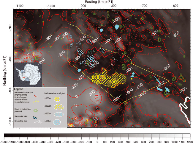
Bedrock topography, and regions where our interpolation scheme replaces BEDMAP PLUS topography. This region is defined in part by the availability of ice thickness measurements and how much they differ from the published interpolation. Green contours denote locations where enclosed basins in the hydrologic potential are present. Hatching indicates areas where bedrock DEM from this study differs from BEDMAP Plus DEM by >250 m.
2. Study Region and Scope
MacIS has an active subglacial water system containing eight subglacial lakes, which we number from the grounding line upstream as Mac1, Mac2, etc. (Fig. 2). The activity of the lakes in the system was reported by Reference Smith, Fricker, Joughin and TulaczykSmith and others (2009) using ICESat laser altimetry; the downstream portion was studied in detail by Reference Fricker, Scambos, Carter, Davis, Haran and JoughinFricker and others (2010) who assimilated ICESat with other remote-sensing data to obtain more accurate estimates of lake volume change. A 2005–06 seismic survey also pointed to subglacial water activity elsewhere on MacIS (Reference Winberry, Anandakrishnan, Alley, Bindschadler and KingWinberry and others, 2009). We treat MacIS as a closed system surrounded by no-flow boundaries with adjacent ice streams (Reference Le Brocq, Payne, Siegert and AlleyLe Brocq and others, 2009). A preliminary map of water drainage at a coarse (5 km) resolution has a dendritic pattern, with Mac1–Mac5 occupying areas of high water flux (Reference Fricker, Scambos, Carter, Davis, Haran and JoughinFricker and others, 2010). In contrast, the water systems for other ice streams appear anastomosing (i.e. many flows reconnect after branching) and contain major bifurcations, such as the diversion of water from upper Kamb Ice Stream to Whillans and Bindschadler Ice Streams (Reference Anandakrishnan and AlleyAnandakrishnan and Alley, 1997; Reference Johnson and FastookJohnson and Fastook, 2002; Reference Le Brocq, Payne, Siegert and AlleyLe Brocq and others, 2009). These reconnections and diversions make it difficult to couple upstream and downstream processes.
(a) Basal melt rate with contours of hydrologic potential (blue) and ice surface velocity (yellow; Reference Joughin, Tulaczyk, MacAyeal and EngelhardtJoughin and others, 2004; contours at 50, 100, 250 and 500 m a−1).(b–e) Hydrologic potential as determined from correlated local minima along RES flight-lines, with location maps inserted. Hydrologic potential decreases monotonically except at subglacial lakes for all flow paths as determined through methods described in Section 4.1.2.

Our study does not address the physical mechanisms of flood initiation and termination (e.g. Reference Evatt, Fowler, Clark and HultonEvatt and others, 2006; Reference FowlerFowler, 2009), nor does it try to identify a particular flow mechanism (i.e. focused conduits versus distributed sheets/cavities; e.g. Reference Flowers and ClarkeFlowers and Clarke, 2002; Reference Creyts and SchoofCreyts and Schoof, 2009; Reference SchoofSchoof, 2010). Also, we do not directly address the relationship between the water system and the flow of overlying ice. We do, however, explore the feasibility of using existing data to test models that include these mechanisms. First, we show how improved analysis of the input data, in spite of uncertainties, can be used to parameterize, tune and validate a simple model of basal water distribution. We then use the data to evaluate several long-held hypotheses (described in the next section) about the transport and distribution of basal water. We acknowledge that there is room for further data analysis and more realistic models. We aim to show, however, that even a simple model can explain recent geophysical observations related to subglacial water flow.
The first question we address is: Do subglacial lakes beneath ice streams and outlet glaciers obtain most of their water from local sources or from distant sources? Many subglacial lakes are located in or immediately downstream of areas of high basal melt associated with geothermal anomalies (e.g. volcanoes) or ice-dynamical anomalies (e.g. ‘sticky spots’ – regions of enhanced basal friction (Reference Blankenship, Bell, Hodge, Brozena, Behrendt and FinnBlankenship and others, 1993, Reference Blankenship, Alley and Bindschadler2001; Reference Bell, Studinger, Shuman, Fahnestock and JoughinBell and others, 2007; Reference Siegert, Le Brocq, Payne, Hambrey, Christoffersen, Glasser and HubbardSiegert and others, 2007; Reference Carter, Blankenship, Young and HoltCarter, 2009a; Reference Smith, Fricker, Joughin and TulaczykSmith and others, 2009; Reference Fricker, Scambos, Carter, Davis, Haran and JoughinFricker and others, 2010; Reference Sergienko and HulbeSergienko and Hulbe, 2011); Fig. 2). It is unclear, however, whether these zones of enhanced melting are the primary water source for lakes or whether the lakes receive much of their water from diffuse sources throughout the catchment. Also, it has been hypothesized that water transport from areas of high melt to areas of net basal accretion downstream is responsible for basal lubrication where the ice would otherwise freeze to the bed (Reference Parizek, Alley, Anandakrishnan and ConwayParizek and others, 2002). In this study, the lakes farthest downstream are adjacent to areas where basal accretion is predicted (Reference Joughin, Tulaczyk, MacAyeal and EngelhardtJoughin and others, 2004; Fig. 2). If the observed volume change for these lakes is consistent with meltwater sourced from the entire basin, then we have more observations to support this hypothesis.
The second question we address is: What fraction of water in the subglacial system is subject to temporary storage in subglacial lakes? If this fraction is large, then we can conclude that subglacial lakes play a major role in the dynamic distribution of basal water. Additionally, if sub-glacial lakes temporarily impound a large enough fraction of the water passing through them, then observations of lake-filling and -draining events can be used to validate more complex models of sub-ice-sheet hydrology (e.g. Reference Flowers and ClarkeFlowers and Clarke, 2002; Reference Parizek, Alley, Anandakrishnan and ConwayParizek and others, 2002; Reference SchoofSchoof, 2010). Furthermore, if the flow mechanism for subglacial floods is qualitatively different from that which is assumed to transport subglacial water in a steady-state system, this could have implications for the relationship between basal sliding and water supplied from upstream (Reference KambKamb, 1987; Reference SchoofSchoof, 2010).
3. Data and Data Preparation
Our model requires three inputs: hydrologic potential, basal melt rate and a time series of volume-change estimates for each subglacial lake in the system. Hydrologic potential is estimated from ice surface elevations derived from ICESat and Moderate Resolution Imaging Spectroradiometer (MODIS) data (Fig. 3) and ice thicknesses derived using data from a combination of radio-echo sounding (RES) and seismic surveys spanning 1957–2005 (Reference Bentley and OstensoBentley and Ostenso, 1961; Reference DrewryDrewry, 1975; Reference Blankenship, Alley and BindschadlerBlankenship and others, 2001). Basal melt rates are obtained from the results of a published temperature model of the area (Reference Joughin, Tulaczyk, MacAyeal and EngelhardtJoughin and others, 2004). The time series of lake volumes come from ICESat and MODIS (Reference Smith, Fricker, Joughin and TulaczykSmith and others, 2009; Reference Fricker, Scambos, Carter, Davis, Haran and JoughinFricker and others, 2010). Below we describe in detail the generation of the model inputs from these datasets.
(a) Map showing locations and types of data used forthis study. The surface elevation is derived from a photoclinometric DEM that uses MOD IS shading to interpolate elevation points from ICESat surface altimetry (Reference Haran and ScambosHaran and Scambos, 2007; T. Haran and others, http://nsidc.org/data/nsidc-0280.html). Surface velocities are obtained from an InSAR analysis by Reference Joughin, Tulaczyk, Bindschadler and PriceJoughin and others (2002). Lake locations and shoreline dimensions come from three separate studies. Ice thickness comes from multiple RES and seismic campaigns, most of which were performed between 1993 and 2005, with earlier campaigns used primarily to fill in blank areas. Grounding line is from J. Bohlander and T. Scambos, nsidc.org/data/atlas/news/antarctic_coastlines.html. (b) A schematic diagram showing how we perform bedrock interpolation. Cells with satisfactory values are blue. Cells with unsatisfactory values are green. A star marks the cell of interest. Black linesborder cells in the same row or column as the cell of interest. White hash lines indicate cells used for interpolation; the basis for selecting these cells is given in Section 4.1.1.

3.1. Hydrologic potential
Hydrologic potential is determined by the water elevation and pressure, and exerts a first-order control on the subglacial water distribution: water flows from high to low potential. In Antarctica the subglacial water pressure is usually assumed to be equal to the overburden or lithostatic pressure (Reference Vogel and TulaczykVogel and Tulaczyk, 2006; Reference Le Brocq, Payne, Siegert and AlleyLe Brocq and others, 2009). Although the overburden pressure can exceed the actual water pressure by up to 200 kPa in fast-flowing regions (Reference Engelhardt and KambEngelhardt and Kamb, 1997), the assumption that water pressure is equal to overburden is sufficient for our study.
Hydrologic potential, θ h, was calculated as
Where z srf is the ice surface elevation, ρ i and ρ w are the densities of ice and fresh water, respectively, and h i is the ice thickness. Therefore the two datasets needed to construct hydrologic potential over a region are the ice surface elevation and the ice thickness. Below we describe how we obtained these two datasets for MacIS.
3.1.1. Ice surface elevation
We estimated ice surface elevation from a 250 m resolution DEM derived from ICESat laser altimetry, acquired between 2003 and 2004 and enhanced with MODIS photoclinometry (Reference Haran and ScambosHaran and Scambos, 2007). The nominal accuracy of this DEM is 1–2 m; however, at the 5 km resolution of our model grid this error is substantially lower.
Estimation of the hydrologic potential requires generating DEMs that optimize the use of data in well-sampled regions while minimizing artifacts in regions where ice thickness data are sparse. The DEMs used to generate hydrologic potential surfaces in this study averaged multiple measurements for gridcells where such measurements existed and interpolated for cells where no measurements existed. Although the dependence of the hydrologic gradient on the ice surface gradient is about ten times greater than the dependence on the bed gradient, the latter can locally exceed the former by an even larger factor (Reference ShreveShreve, 1972). Thus, although the regional flow of subglacial water is controlled primarily by the ice surface gradient, bedrock topography could exert an important control on the local water flow. It is possible that features smaller than the 5 km grid resolution could control local water routing and in some places change the regional water routing, as demonstrated in recent models (Reference Wright, Siegert, Le Brocq and GoreWright and others, 2008).
3.1.2. Ice thickness
We estimated ice thickness using a combination of RES and seismic surveys spanning 1957–2005. Along-track resolution varied from 3 km for the earlier Scott Polar Research Institute/ US National Science Foundation/Technical University of Denmark (henceforth SPRI) surveys (Reference DrewryDrewry, 1975) to <10 m for the most recent University of Texas Institute for Geophysics Thwaites Catchment survey (UTIG-THW) (Reference Holt, Blankenship, Morse, Young, Peters, Kempf, Richter, Vaughan and CorrHolt and others, 2006). Most of the data from the remaining UTIG Support Office for Aerogeophysical Research (UTIG-SOAR) surveys had an along-track spacing of ∼30 m (Reference Blankenship, Alley and BindschadlerBlankenship and others, 2001). In areas where there were no RES data we used measurements from seismic traverses associated with the first International Geophysical Year (Reference Bentley and OstensoBentley and Ostenso, 1961; Reference Bentley, Chang and CraryBentley and Chang, 1971). Where neither RES nor seismic data were available, we relied on interpolation strategies described by Reference Lythe and VaughanLythe and others (2001) for the BEDMAP compilation and on subsequent improvements from the BEDMAP Plus database (Reference Pritchard, Arthern, Vaughan and EdwardsPritchard and others, 2009). In merging a variety of data sources, we considered both the uncertainty at the time of measurement and the possibility that ice thickness has subsequently changed. The uncertainty in ice thickness may be as large as 50 m in areas of steep bedrock topography, but is much lower for the low-relief areas under most of MacIS (Table 1). To estimate decadal changes in ice thickness we used published results from two independent satellite techniques: satellite radar altimetry (Reference Wingham, Siegert, Shepherd and MuirWingham and others 2006b) and mass flux measurements (Reference RignotRignot and others, 2008), which unfortunately extended back only to 1992. Both techniques suggested that the maximum local rate of surface change was ∼0.1 m a−1 for 1992–2008. Satellite laser altimetry (Reference Pritchard, Arthern, Vaughan and EdwardsPritchard and others, 2009) confirms this magnitude for 2003–08. This may introduce an error of up to 1 m in ice thickness for the faster-flowing portions of MacIS and up to 5 m for the interior. While all these errors sum up to a total of 60 m of ice thickness, this value is multiplied by g(1 – ρ I/ρ w) such that when it is added to the uncertainties from surface elevation we get a maximum error ±60 kPa, with the largest contribution from ice thickness errors in regions of steep bedrock topography.
Data sources used

Comparison of ice thickness data from BEDMAP Plus with those from recent RES campaigns revealed that they contain errors of >500 m. Thus it was not possible to seamlessly blend the higher-resolution line data with the original interpolation for the central part of our study area (Fig. 1). To remedy this, we have used the misfit between measurements and the DEM to define an area in which to perform interpolation. Our hybrid algorithm combined the best features of bilinear and inverse-distance-weighting interpolation. Given the nonuniform distribution of ice thickness measurements, a simple inverse-distance weighting risks averaging too many values from a small region. Our algorithm identified eight nearby gridcells for which the ice thickness was based on a measurement. Two of these were in the same row, one on each side of the cell in question, and two others were in the same column, again with one on each side. The four remaining cells are the nearest cells with a satisfactory bed elevation in each of the quadrants formed by two vectors along the row and column of the cell in question (Fig. 3b). We used the inverse-distance-weighted average bed elevation from each of these eight cells to determine the bed elevation for a given cell. The resulting interpolated bed topography was then continuous with the well-measured topography, allowing us to further parameterize subglacial lakes and channels.
3.2. Basal melt rate
Our model assumes that all water enters the system as basal melt. We used the basal melt map of Reference Joughin, Tulaczyk, MacAyeal and EngelhardtJoughin and others (2004), which showed that MacIS is unique among Siple Coast ice streams in that much of the melt occurs in the fast-flowing downstream region (Fig. 2). This is due in part to the presence of large ‘sticky spots’ (Reference MacAyeal, Bindschadler and ScambosMacAyeal and others, 1995), which convert gravitational potential energy into frictional melting. Reference Fricker, Scambos, Carter, Davis, Haran and JoughinFricker and others (2010) suggested that the high basal traction at these sticky spots would provide water from shear heating of the overlying ice, and that the contrast in basal traction would form a surface depression with consequent lowering of the hydrologic potential downstream of the sticky spot, resulting in the observed subglacial lake distribution. More detailed modeling by Reference Sergienko and HulbeSergienko and Hulbe (2011) has shown that localized areas of enhanced basal traction will create local minima in the downstream hydrologic potential where water will collect. Whether or not basal melt from these sticky spots is sufficient to explain observed lake volume changes is one of the questions addressed in this paper. For our error estimates we used the published value for basin-wide melt of ±10% (Reference Joughin, Tulaczyk, MacAyeal and EngelhardtJoughin and others, 2004).
There were two limitations in our model that result from (1) differences between the modern DEMs used in our study and the BEDMAP DEM used by Reference Joughin, Tulaczyk, MacAyeal and EngelhardtJoughin and others (2004) and (2) the assumption that the melt rate was constant over the study period. Recent high-resolution DEMs for surface and bed elevation have revealed greater topographic detail than the BEDMAP DEM; differences are up to 500 m at some grid nodes (Fig. 1). The resulting differences in surface slope and thickness, however, appeared to average out over the basin and thus affected the actual spatial distribution of basal melt, but not the total volume of meltwater. Given that rates of lake-volume change integrate meltwater generated over spatial scales of ten ice thicknesses or greater (Reference Joughin, Tulaczyk, MacAyeal and EngelhardtJoughin and others 2004), we considered these modeled melt rates to be sufficient for our study.
The assumption of constant melt rate over the study period may not be valid since changes in the melt rate could result from the passage of water along the interface (Reference Creyts and ClarkeCreyts and Clarke, 2010), and water flowing up adverse bed slopes may require more heat than is available from turbulent heating and thus freeze out in places. Also, variations in the thickness of the water layer will influence its ability to conduct basal heat to the overlying ice. Simulating these processes, however, would have required a more complex water model, introducing additional uncertainty. Additionally, work by Reference Carter, Blankenship, Young and HoltCarter and others (2009a) on a flood in Adventure Subglacial Trench showed that, for the low hydraulic gradients in much of the Antarctic ice sheet, the fraction of water gained and lost to hydrodynamic melting and freezing accounts for <1% of the total water budget.
3.3. Lake locations and volume-change estimates
We used the locations of eight ICESat-detected lakes (Mac1–Mac8; Reference Smith, Fricker, Joughin and TulaczykSmith and others, 2009; Reference Fricker, Scambos, Carter, Davis, Haran and JoughinFricker and others, 2010). We used estimates of volume changes from two published ICESat studies: for Mac1–Mac5, we used the estimates reported by Reference Fricker, Scambos, Carter, Davis, Haran and JoughinFricker and others (2010), which incorporated MODIS image data and had a maximum error of ±20%; for Mac6–Mac8 we also used estimates from Reference Smith, Fricker, Joughin and TulaczykSmith and others (2009). All ICESat time series were limited to the epochs of the ICESat acquisition campaigns, which were every 3–4 months. Additionally, there are two downstream lakes which were inferred through seismic monitoring of a subglacial flood in 2005 (Win1 and Win2 in Fig. 2; Reference Winberry, Anandakrishnan, Alley, Bindschadler and KingWinberry and others, 2009). Although there are no ICESat time series available over these lakes, we will show that their locations were useful for validating and evaluating our model.
In assuming that water is stored only in known lakes, we neglected potential storage elsewhere in the subglacial hydrologic system. Some models suggest that water can be stored in the subglacial till (Reference Tulaczyk, Kamb and EngelhardtTulaczyk and others, 2000) and within the water sheet itself (Reference Creyts and SchoofCreyts and Schoof, 2009). Although these phenomena have been observed in bore-holes (Reference Engelhardt and KambEngelhardt and Kamb, 1997), neither is currently observable on the spatial scale of the MacIS catchment. This assumption, like others, kept the model simple and testable against current observations.
4. Methods
4.1. Subglacial lakes and predicted flow paths
To incorporate the effects of sub-gridscale topographic features on water routing and distribution, we designed an algorithm to follow the most prominent drainages, borrowing from an established Geographic Information System (GIS) technique of stream etching into DEMs (Reference Saunders, Maidment and DjokicSaunders, 2000). We used the ‘law of V’s’ (Reference Dupain-TrielDupain-Triel, 1791) to identify a proto-drainage. We then determined the intersection between this proto-drainage and ground tracks of the RES ice thickness data. We used the position and head of the nearest local minimum in the hydrologic potential along the flight-line as a point in the drain path (Fig. 2). We interpolated the hydrologic potential, the x and y position of the intersections of the drainage and flight-line, the bedrock elevation, the ice thickness and the surface elevation along this path using a piecewise cubic hermitic polynomial to preserve monotonicity between data points. The hydrologic potential for all gridcells containing points of any drain path was then set to the mean of those points. If two drain paths were within two gridcells of one another but did not intersect, we altered the bed topography in some locations to prevent leaking and to better incorporate small observed barriers in the hydrologic potential, as determined by the original RES data. Figure 2 shows all places where this tuning is done.
Despite these improvements, the resulting hydrologic potential surface still contained many enclosed basins or ‘holes’. Reference Johnson and FastookJohnson and Fastook (2002) reported similar results and tried to associate these basins with subglacial lakes, a number of which were later confirmed by geophysical data (Reference Siegert, Carter, Tabacco, Popov and BlankenshipSiegert and others, 2005; Reference Bell, Studinger, Shuman, Fahnestock and JoughinBell and others, 2007; Reference Carter, Blankenship, Peters, Young, Holt and MorseCarter and others, 2007). For this study we worked only with lakes confirmed by previous geophysical studies. We differentially adjusted the hydrologic potential by raising the bed elevation of all holes, including those associated with known lakes, until there was a monotonically decreasing path in the hydrologic potential from every cell in the domain to the grounding line. Using this final version of the hydrologic potential, we parameterized the filling and draining of lakes in our flow model, as discussed next.
4.2. The flow model and subglacial lakes
For all gridcells lying outside a filling subglacial lake we prescribed water fluxes as
Where Q in and Q out are the incoming and outgoing water flux, m is the basal melt rate (negative if water is freezing to the base) and Δx and Δy are the horizontal dimensions. Flux was distributed among the eight neighboring cells using the D8 routing algorithm (Reference Quinn, Ostendorf, Beven and TenhunenQuinn and others, 1998); cells with higher hydrologic potential received no flux, while cells with lower hydrologic potential received a fraction of the outflow, proportional to the local slope of the hydrologic potential surface:
with k being the number of adjacent cells with lower hydrologic potentials, and s the distance to the adjacent cell (Δx, Δy or ![]() ). Reference Le Brocq, Payne and SiegertLe Brocq and others (2006) explored variants of this routing scheme.
). Reference Le Brocq, Payne and SiegertLe Brocq and others (2006) explored variants of this routing scheme.
4.3. Lakes as sinks and sources
We aimed to determine whether the estimated regional basal melt rate (Reference Joughin, Tulaczyk, MacAyeal and EngelhardtJoughin and others, 2004) and the observed filling and draining of subglacial lakes were sufficient to explain the observed behavior of lakes downstream. In essence, we used the ICESat-derived time series of lake-drainage events to simply parameterize lake-drainage events and used the ICESat-derived time series of lake-filling events to validate the transport and melt model. We do not presume to know the exact mechanism by which subglacial floods are initiated; hypotheses for possible mechanisms are described elsewhere (Reference Evatt and FowlerEvatt and Fowler, 2007; Reference Carter, Blankenship, Young and HoltCarter and others, 2009a; Reference FowlerFowler, 2009). Our simple model did not account for details related to channel geometry and water-pressure evolution and its impact on sliding. Nonetheless, if a simple model can show consistency among estimates for basal melt, observed lake volume changes and ice-surface and ice-bed topography, it may be possible to use observations of lake volume change to test more complex models. Also, this simple model served to validate hypotheses relating to the source regions for the subglacial lakes of MacIS.
For simplicity, we focused on the five lakes undergoing the largest volume changes in the catchment, Mac1–Mac5. We considered Mac6–Mac8 only for the purpose of quantifying discharge variability over time. The procedure was as follows: Any gridcell lying within the boundaries of a subglacial lake could be in one of two states: filling or draining. We considered a lake to be draining if and only if the volume change during a given interval was negative with a magnitude greater than 3 m3 s−1. We excluded events during which the apparent volume loss might be due to ICESat sampling issues, such as for Mac1 between November 2006 and March 2007. If the drainage condition was not met, or if there was no volume change during the interval, then we assumed that the lake was filling (Fig. 4). For filling lakes, water entering the lake perimeter increased the lake volume and did not leave the gridcell. For a draining lake, we allowed incoming water to pass through. We accounted for the downstream transfer of water following a lake drainage by dividing the volume change by the time interval and gridcell size and treating the result as a source for the gridcells immediately downstream.
Volume change over time for lakes Mac1–Mac5 adapted from Reference Fricker, Scambos, Carter, Davis, Haran and JoughinFricker and others (2010; reprinted with permission). We have highlighted portions of the plot that correspond to lake drainage events for which the volume loss is >3 m3 s−1. We also neglect short events that may be artifacts of sampling errors, such as the drainage of Mac1 between November 2006 and March 2007.

In addition to a model run involving ICESat-observed filling and draining events, we also performed two control experiments to test the locations of the observed lakes with respect to modeled discharge and determine how their distribution might influence water availability downstream: one with no lakes, the other with all lakes filling. The ‘lake-free’ run was similar to the steady-state basal water model of Reference Le Brocq, Payne, Siegert and AlleyLe Brocq and others (2009), except that it used more detailed bedrock topography and a simplified version of the routing algorithm. This run had a steady water distribution for a given melt rate and hydrologic potential, and the only sink was the Ross Sea. In the ‘all-filling’ run, we treated all lakes as sinks, both to see the areas where lakes will limit water availability and to test whether the observed filling rates can be reproduced entirely by meltwater from local sources (i.e. geothermal or frictional heating anomalies).
5. Results
5.1. Flow paths identify subglacial lakes as hydrologic potential basins
An analysis of the RES line data indicated that there is a unique path of steepest descent on the hydrologic potential surface between every known subglacial lake in the study area and the grounding line. The monotonicity of this path was broken only at known subglacial lakes (Fig. 2). Given that our calculation of hydrologic potential neglected effective pressure and the observed surface elevation change over subglacial lakes (Reference Fricker, Scambos, Carter, Davis, Haran and JoughinFricker and others, 2010), we expected some enclosed depressions along the flowlines as they crossed subglacial lakes. There were no other departures from monotonicity along any flow paths. Reference Johnson and FastookJohnson and Fastook (2002), who dealt exclusively with geometry from gridded datasets, identified many enclosed basins in the hydrologic potential that were later found to correlate with subglacial lakes. Our examination of the original RES line data provided strong support for the hole-filling algorithms of Reference Johnson and FastookJohnson and Fastook (2002) and Reference Le Brocq, Payne, Siegert and AlleyLe Brocq and others (2009).
5.2. Control runs (lake-free and all-filling)
Our lake-free model (Fig. 5a) differs from the models of Reference Johnson and FastookJohnson and Fastook (2002) and Reference Le Brocq, Payne, Siegert and AlleyLe Brocq and others (2009), primarily because we used different DEMs for the surface and elevation topography. This results in a stronger correlation between subglacial water distribution and the location of known subglacial lakes. The all-filling run showed a strong correlation between an abrupt increase in along-flow discharge and the presence of subglacial lakes. The meeting of several tributaries upstream of Mac4 and Mac5 appears responsible for their existence. In contrast, as pointed out by Reference Fricker, Scambos, Carter, Davis, Haran and JoughinFricker and others (2010), Mac1–3 are all close to regions of high basal melting provided by increased friction at sticky spots. All but one of the lakes occupied areas with a high steady discharge; the exception was Mac6 which lost water throughout the ICESat mission. If it filled, it may have done so at a rate below that detectable by ICESat. Thus our observed lake distribution was qualitatively consistent with the measured topography and inferred melt rate: lakes exist at hydropotential lows in areas of high basal water flux. These lakes have a large impact on the availability of water to downstream locations, despite their small spatial extent. This impact was clear in our all-filling run, in which water was nearly absent for tens of km downstream of all lakes (Fig. 5b).
Steady-state water flux with (a) lake-free run and (b) all-filling run. Note logarithmic color scale.

5.3. Flow evolution with time
The time-lapse plots of modeled water distribution from March 2004 to March 2008 showed an early period of high discharge (March–June 2004; Fig. 6a). Water draining from Mac5 passes through Mac4 into Mac3, subsequently arriving at Mac1 (Fig. 6). The ICESat temporal sampling is insufficient to determine the exact timing of the draining/filling of the three lakes, except for Mac5, which appears to have started to drain before Mac3 and Mac1. During this period there was relatively more water supplied to the bed between Mac3, Mac4 and Mac5 (Fig. 6a). If the steady flow from Mac1 was real (i.e. not an artifact of our lake-volume averaging algorithm or surface change associated with dynamic effects (Reference Sergienko, MacAyeal and BindschadlerSergienko and others, 2007)), then the water supplied by this event appears to have been enough to keep the bed downstream of Mac1 well lubricated for nearly 9 months after the end of discharge from other lakes (Fig. 6b–d). From June to November 2005, much of the bed below Mac1 had only local water supply (Fig. 6e). As our model did not consider changes in transmissivity or in storage outside lakes, we cannot assess whether other mechanisms may have lubricated the bed during this period. Water stored in subglacial sediments, however, is likely to help maintain lubrication, releasing water during dry periods and retaining it during subglacial floods (Reference Tulaczyk, Kamb and EngelhardtTulaczyk and others, 2000). From November 2005 until March 2006, the regions between Mac2 and Mac1 and between Mac4 and Mac3 both had water influx following discharge from Mac2 and Mac4, respectively (Fig. 6f). The flood wave from Mac4 can then be seen passing from Mac3 to Mac1 between March 2007 and October 2007 (Fig. 6g–h). In all runs, almost all water in the catchment appears to have passed through Mac1.
Maps of modeled evolution of water distribution over time, forced with the lake volume-change time-series data from Reference Fricker, Scambos, Carter, Davis, Haran and JoughinFricker and others (2010) with time intervals selected to coincide with ICESat campaigns (line colors in inserts same as Fig. 4): (a) March–June 2004, (b) June–October 2004, (c) October 2004–March 2005, (d) March–June 2005, (e) June–November 2005, (f) November 2005–March 2006, (g) March–June 2006, (h) June–November 2006, (i) November 2006–March 2007, (j) March–October 2007 and (k) October 2007–March 2008. Note different color scale from previous figure.

5.4. Discharge variability over time
In the fastest-flowing regions of MacIS, where surface velocity exceeds 250 m a−1, the range in modeled discharge values exceeded the steady-state discharge by an order of magnitude (Fig. 7). In some areas, such as downstream of Mac4 and Mac5, the water supply depended almost entirely on the dynamics of one or two lakes. Discharge in these areas ranged from near zero to >20 m3 s−1 per 25 km2 gridcell. In other areas, such as upstream of Mac1, the presence of multiple nearby lakes maintained a more consistent water supply. Upstream lakes such as Mac7 appear to have strongly influenced the water available for the tributary region downstream (Fig. 7).
(a) Range of discharge values from model (maximum–minimum). (b) Log ratio of flux variability to steady-state control flux.

5.5. Winberry lakes
In all model runs, the lakes of Reference Winberry, Anandakrishnan, Alley, Bindschadler and KingWinberry and others (2009) received only a small amount of water, roughly 0.13–0.19 m3 s−1. If flooding were to have occurred for just 10 min every 2 weeks (as observed by the seismic array) with no interim leakage, then the average discharge rate during the flood would have been ∼300 m3 s−1 . Applying the Reference Walder and FowlerWalder and Fowler (1994) model to this channel, as described by Reference Carter, Blankenship, Young, Peters, Holt and SiegertCarter and others (2009b), we find that the channel would need to be substantially larger than inferred by Reference Winberry, Anandakrishnan, Alley, Bindschadler and KingWinberry and others (2009) to carry this flow. If, however, the discharge was ∼100 m3 s−1 with large sediment (∼1 mm), then a channel 80 m wide and 70 cm deep could have delivered the required flow and fall within the range of seismically inferred channel geometries. Given the DEM sampling errors relative to the small catchment feeding these lakes and the short event duration (2 weeks) relative to ICESat temporal sampling (3–4 months), it is promising that the channel dimensions predicted by our model were within an order of magnitude of those inferred through seismic analysis (Fig. 2e).
5.6. Water budgets
Observed volume changes can account for all the meltwater produced in the MacIS catchment. This agreement between modeled and observed lake volume changes was impressive, given the simplicity of our model. This result makes us optimistic that more sophisticated subglacial water models (in which parameters such as conduit geometry, hydrologic conductivity, sediment storage and water temperature evolve over time) will be able to simulate observed volume changes if sufficient data are available (e.g. ice surface and bedrock geometry, ice surface velocity and lake distribution). Below we explore the differences between modeled and observed volume changes and speculate on modeling and data improvements that could resolve these discrepancies.
5.6.1. Mac3, Mac4 and Mac5
Our model did not reproduce observed filling rates for either Mac4 or Mac5 (2.1 ± 0.4 m3 s−1 and 5.3 ± 1 m3 s−1, respectively) for any time interval. However, the combined modeled filling rate of the two lakes (7.3 m3 s−1) closely matched the combined observed rate for June–November 2005. The difference between modeled and observed volume change was <0.05 km3, or ∼13% of the total volume change, which is comparable to the ∼20% error in the volume estimates. The difference between modeled and observed volume change was of the same magnitude as the volume change for Mac6 and Mac7 (Fig. 8a). Even when the filling of Mac3 is included in our water budget, we maintained good agreement between the modeled rate of 11.7 m3 s−1 and observed rates of total volume change during both the beginning and end of the observation period (10.2 ± 2 m3 s−1 and 13 ± 2.6 m3 s−1, respectively). We were unable, however, to account for all the water in the system during a Mac4 drainage event from November 2005 to March 2006. This disagreement is not surprising, given that the model assumed instantaneous downstream transport and did not account for other means of water storage. Changes in ice till porosity (Reference Tulaczyk, Kamb and EngelhardtTulaczyk and others, 2000) and water layer thickness (Reference Creyts and SchoofCreyts and Schoof, 2009) could account for some of the missing water. Also, since our model did not have explicit lake drainage mechanisms, there may have been unaccounted interactions between Mac4 and Mac5; for example, Reference Fricker, Scambos, Carter, Davis, Haran and JoughinFricker and others (2010) showed evidence of flow back and forth between Mac4 and Mac5.
(a, b) Modeled and observed water budgets for (a) Mac3–Mac5 and (b) Mac1–Mac3. (c) Pie chart showing provenance of water that fills Mac1 between June 2005 and November 2007. Resolution of the Mac4 and Mac5 water budget is more effective if both lakes are treated as parts of a single combined lake.

5.6.2. Mac2
The model produced a volume change for Mac2 of 0.33 km3 between November 2003 and November 2005, compared to an observed volume change of 0.3 km3 +20% (Fig. 7b). On shorter timescales, however, the modeled and observed volume changes differed by larger amounts. Observations showed that most water arrives between March 2005 and November 2005, whereas the model predicted steady filling for most of the longer period. We attribute this discrepancy to our assumption that water was stored only in known lakes. Given the sparse ICESat track spacing and the paucity of RES data upstream of Mac2, it is possible that there was a subglacial lake upstream which could have stored the unaccounted water. Increased till porosity or changes in the upstream mean water thickness could have provided additional storage upstream of Mac2. Modeling by Reference Creyts and SchoofCreyts and Schoof (2009) suggests that water sheets could undergo thickness changes of ∼0.1 m due to subtle regional pressure changes. Such changes occurring over a 50 km × 50 km area upstream of Mac2 between March and November 2005 could have generated the observed volume increase, which would not have been detectable by ICESat repeat-track analysis or MODIS image differencing. Another possible source of discrepancy is that there was an unexpectedly large modeled volume increase caused by apparent leakage of water from the Mac3–Mac5 system between March and June 2004. Although a distributed drainage system could potentially radiate into several different flow paths (Reference RobertsRoberts, 2005), it is unclear if this was the case here.
5.6.3. Mac1
The modeled volume increase for Mac1 was 0.71 km3 from June 2005 to March 2008, which was consistent with the observed volume change of 0.69 ± 0.14 km3 (Fig. 8b). We considered how the Mac1 water sources combine to account for the observed filling (Fig. 8c). More than half the water comes directly from Mac3, with an additional 21% from Mac2. We can attribute 20% of the volume change to water upstream of Mac2 and Mac3 passing through them as they drain. Only 8% of the volume change is attributed to basal melt associated with shear heating at a sticky spot immediately upstream. As with other lakes, there are timing differences of up to 4 months between modeled and observed volume changes. We may also be observing an artifact of estimating volume changes by averaging repeats of all ICESat tracks across the lake during a 33 day campaign to represent the lake state in the middle of that campaign. All three ICESat tracks across Mac1 show monotonically increasing surface elevation. In particular, the track farthest downstream (track 355) shows at least 0.5 m of surface rise (Reference Fricker, Scambos, Carter, Davis, Haran and JoughinFricker and others, 2010). The downstream portion of the lake may maintain a constant pool of water, while water depths in the upper parts of the lake are more variable. We found that Mac1 volume fluctuations depended on the dynamics of upstream lakes; much of the water that passed through this lake originated far upstream.
6. Discussion
6.1. Open or closed system?
The combined water budget for Mac3–Mac5 shows a nearly linear monotonic increase in total water storage between June 2004 (at the end of the Mac3 flood) and November 2006 (the start of the next flood). This suggests that a majority of the upstream water passes through these three lakes, with little leakage. There is some indication, however, that the filling rate decreased with time. One explanation for this is that lakes upstream were storing water that would otherwise feed this system, although we expect this amount to be small. Reference Smith, Fricker, Joughin and TulaczykSmith and others (2009) reported that Mac7 (labeled ‘Bindschadler 5’ in that study) received ∼0.03 km3 a−1 between October 2003 and October 2007, an amount equivalent to the reduced filling of the Mac3–Mac5 system. Mac6 lost 0.05 km3 during the same period (Reference Smith, Fricker, Joughin and TulaczykSmith and others, 2009). If the majority of the loss from Mac6 occurred between June 2004 and November 2006, then the filling rates for Mac3– Mac5 would have been higher than modeled rates.
6.2. Local versus regional sourcing
There is some debate as to whether subglacial lakes obtain water from local or distant sources (Reference Bell, Studinger, Shuman, Fahnestock and JoughinBell and others, 2007; Reference Bindschadler and ChoiBindschadler and Choi, 2007; Reference Fricker and ScambosFricker and Scambos, 2009). Subglacial lakes near ice divides exist, in part, as a result of high geothermal flux and the presence of hydrologic potential basins (Reference SiegertSiegert, 2000; Reference Tikku, Bell, Studinger, Clarke, Tabacco and FerraccioliTikku and others, 2005; Reference BellBell, 2008; Reference Carter, Blankenship, Young, Peters, Holt and SiegertCarter and others, 2009b). For ice-stream regions, however, the lakes could not have behaved as observed without receiving water from the wider catchment. Of the five MacIS lakes farthest downstream (Mac1–Mac5), only Mac5 appears to have been filled by constant hydrologic flux. The other lakes, even those with no known lakes upstream, appear to have filling rates that were influenced by the episodic storage and release of water from upstream lakes. As the flooding of these lakes depends in part on their filling rate (Reference Evatt, Fowler, Clark and HultonEvatt and others, 2006), the water distribution downstream will be the sum of many interrelated events and will be nonlinear over time. Several modelers have tried to link lake formation with high melt rates at sticky spots (Reference Stokes, Clark, Lian and TulaczykStokes and others, 2007; Reference Sergienko and HulbeSergienko and Hulbe, 2011). This study does not refute that enhanced frictional melting may play a role in lake formation beneath fast-moving ice masses, but it does suggest that observed lake behavior in fast-flowing areas cannot be explained by local melt sources alone. Indeed, if the nearest sticky spot were the sole source of meltwater for Mac1, the resulting surface elevation change would have been <1 m over the ICESat period and might not have been identified. It is possible that the traction contrast across sticky spots creates many small lakes that are not detectable with ICESat. The lakes in the inventory of Reference Smith, Fricker, Joughin and TulaczykSmith and others (2009) may have been only a subsample of lakes that were either draining at the time or were fed by a large hydrologic catchment basin.
The volume change for the downstream lakes shows a clear link to upstream lakes and to meltwater produced throughout the basin. We can thus confirm with observations what models have shown (Reference Parizek, Alley, Anandakrishnan and ConwayParizek and others, 2002; Reference Le Brocq, Payne, Siegert and AlleyLe Brocq and others, 2009): that subglacial water in fast-flowing areas is transported from areas of net basal melting to areas of net accretion.
6.3. Subglacial lake floods dominate the water budget in fast-flow regions
A map of ice velocity and discharge variability for the MacIS drainage basin shows that >55% of ice moving at 250 m a−1 or faster is underlain by a highly variable subglacial water system (Fig. 7). Given that Bindschadler, Whillans and Mercer ice streams also have several active subglacial lakes, as do most fast-flowing outlet glaciers in Antarctica (Reference Fricker, Scambos, Bindschadler and PadmanFricker and others, 2007; Reference Smith, Fricker, Joughin and TulaczykSmith and others, 2009), we can assume that subglacial floods influence the basal water distribution in these other regions. Much research has explored the links between water distribution and basal sliding for ice sheets (e.g. Reference WeertmanWeertman, 1972; Reference FowlerFowler 1986; Reference Iken and BindschadlerIken and Bindschadler, 1986; Reference AlleyAlley, 1989; Reference Tulaczyk, Kamb and EngelhardtTulaczyk and others, 2000; Reference Arnold and SharpArnold and Sharp, 2002; Reference Johnson and FastookJohnson and Fastook 2002; Reference Le Brocq, Payne, Siegert and AlleyLe Brocq and others, 2009; Reference SchoofSchoof 2010; Reference Pimentel and FlowersPimentel and Flowers, 2011). This work has showed that, for basal water in distributed systems where effective pressure decreases with increasing discharge, higher discharges will lead to increased sliding, through softening of the subglacial till or increased separation between the ice and the bed. In contrast, subglacial conduits in which effective pressure increases with discharge will tend to enhance basal traction by efficiently removing basal water from subglacial cavities and till. The subglacial water models that have dealt exclusively with Antarctica and the Siple Coast (Reference Johnson and FastookJohnson and Fastook, 2002; Reference Le Brocq, Payne, Siegert and AlleyLe Brocq and others 2009) have assumed a distributed system in quasi-steady state. This assumption was justified in part because in the Siple Coast ice streams, low ice surface gradients (∼0.1 %) limit the energy available to melt conduit walls, and large ice thicknesses (∼1000 m) create high basal pressures that would close channels rapidly (Reference AlleyAlley 1989, Reference Alley1996). However, recent studies on the evolution of sub-glacial floods in Antarctica (Reference Evatt, Fowler, Clark and HultonEvatt and others, 2006; Reference Evatt and FowlerEvatt and Fowler, 2007; Reference Carter, Blankenship, Young and HoltCarter and others, 2009a; Reference FowlerFowler 2009) have shown that subglacial conduits are a plausible flow mechanism. Although our study does not deal directly with flow mechanisms, it does show that flooding events can account for nearly all the water produced in a subglacial catchment. It also highlights the importance of further study of the mechanisms of flood initiation and water transport, in order to accurately represent the relationship between the sub-glacial water system and the flow of overlying ice.
6.4. Higher-resolution validation and tuning of basal water models
Incorporating subglacial lake volume changes for model runs covering the ICESat period may not require the full physics of subglacial floods, but could be done with the simple parameterization described here. Such a model, however, would apply only to the period of the ICESat campaigns (2003–09), and volume changes would need to be well constrained and independently verified by other data (e.g. GPS, ice surface velocity, RES reflections and MODIS image differencing (e.g. Reference Fricker, Scambos, Carter, Davis, Haran and JoughinFricker and others, 2010)). Furthermore, our method is sensitive to ice surface and bedrock geometry, and therefore requires relatively dense and accurate surface and ice thickness measurements. Unfortunately, data of sufficient quality are currently not available for most of Antarctica.
Evolutionary ice-sheet water models will need to simulate lake formation, filling and drainage in a way that is independent of data on their current distribution. Work by Reference Sergienko and HulbeSergienko and Hulbe (2011) shows promise for demonstrating how traction contrasts associated with sticky spots result in local minima in the ice surface, creating enclosed basins in the hydrologic potential downstream. As water collects, it enhances basal lubrication, increasing the traction contrast in a positive feedback. Whereas the models of Reference Johnson and FastookJohnson and Fastook (2002) and Reference Le Brocq, Payne, Siegert and AlleyLe Brocq and others (2009) manually filled in the local minima in the hydrologic potential, it may be more realistic to have such minima fill, drain and overflow as the ice sheet evolves. We would begin by applying the model described in this study to domain that includes only MacIS and other areas where the data are sufficient for 2003–09 and then expand it to the larger ice-sheet system for longer runs with an evolutionary lake model (e.g. Reference Sergienko and HulbeSergienko and Hulbe, 2011).
The 2003–09 ICESat dataset for MacIS could be useful in developing and testing improved models of subglacial water evolution and lake volume change. When averaged over a period of several years, the modeled filling rates of Mac2– Mac5 were consistent with observations. Higher-order water flow models, which include terms for changes in hydrologic conductivity, dynamic flow system geometry, water storage in subglacial tills, water-pressure evolution and/or water temperature (e.g. Reference Flowers and ClarkeFlowers and Clarke, 2002; Reference Evatt, Fowler, Clark and HultonEvatt and others, 2006; Reference Creyts and SchoofCreyts and others, 2009; Reference SchoofSchoof, 2010), could be applied and tested on the MacIS domain, at least along the flow paths identified here. To date, none of these models has been tested on an actual Antarctic subglacial flood. Also, our analysis of the Reference Winberry, Anandakrishnan, Alley, Bindschadler and KingWinberry and others (2009) flood shows promise for using seismic data to monitor small-scale and short-duration events that may not be detectable with ICESat data. Although no single class of observations or model can explain all subglacial water events in Antarctica, there exist adequate data in many regions to test key elements of models.
Finally, now that we have validated the hypothesis that lakes temporarily impound almost all the water that passes through them, we can resolve a catchment-wide water budget on the scale of individual lakes. Using this principle, we can infer hydrologic connections and bed topography where ice thickness data are sparse, such as at Recovery Glacier (Reference Bell, Studinger, Shuman, Fahnestock and JoughinBell and others, 2007), if the behavior of nearby lakes is correlated. Although RES data are dense in the fast-flowing regions of the Siple Coast, large areas farther upstream remain poorly surveyed. If the modeled behavior of subglacial lakes in the downstream areas is consistent with observations, then we can be more confident about the DEM and basal water distribution upstream.
7. Conclusions
Using a simple steady-state water model, with a published dataset for basal melt rates and adapted DEMs of ice surface and bedrock topography, we have reproduced subglacial lake volume changes estimated from satellite data analysis by Reference Fricker, Scambos, Carter, Davis, Haran and JoughinFricker and others (2010) for individual subglacial lakes in MacIS. For this system, we have validated the hypothesis that subglacial lakes temporarily impound nearly all water that passes through them. Our work provides solid evidence that downstream regions receive the majority of their water from the upper part of the catchment. Furthermore, the subglacial water budget for MacIS is approximately in balance over time.
We have also presented a reproducible means of parameterizing important sub-DEM-scale features in the ice surface and bedrock topography using the original RES line data. By demonstrating that the flow paths determined by this method are monotonically decreasing except where they intersect subglacial lakes, we have given observational justification to a long-practiced but rarely justified technique in which isolated depressions in the hydrologic potential are assumed to be filled.
Our modeling results lay the groundwork for using real data to validate such higher-order water flow models under development (e.g. Reference Creyts and SchoofCreyts and Schoof, 2009). Incorporating subglacial lake volume changes for model runs covering the ICESat period may not require the full physics of subglacial floods, but could be done with the simple parameterization described here. While most current ice-sheet models do not include models for subglacial water transport, this transport has long been invoked to explain observed ice behavior, especially for maintaining basal lubrication in the downstream regions of the Siple Coast ice streams where basal accretion is believed to occur (Reference Joughin, Tulaczyk, MacAyeal and EngelhardtJoughin and others, 2004).
Acknowledgements
ICESat data analysis was funded through NASA Award NNX07AL18G. RES data collection was funded by NASA grant NNX08AN68G. The University of Texas Institute for Geophysics Support Office for Aerogeophysical Research through which many of the RES data in this paper were collected was supported by US National Science Foundation grant OPP-9120464, OPP-9319369. Funding during the analysis and writing was provided by the Scripps Institution of Oceanography Postdoctoral Program and the Institute of Geophysics and Planetary Physics of Los Alamos National Laboratory LLC subcontract No. 73593-001-09. The manuscript was improved by comments from and conversations with H. Pritchard, R. Bindschadler, T. Creyts, J. MacGregor, T. Haran, T. Scambos, C. Jackson and A. Le Brocq.


