


1 Introduction
Unification deals with languages with metavariables. Let us assume that a language with metavariables comes with a well-formedness judgement of the shape
 $\Gamma;a\vdash t$
, meaning that the term t is well formed in the metavariable context
$\Gamma;a\vdash t$
, meaning that the term t is well formed in the metavariable context
 $\Gamma$
and the scope a. What we call a scope depends on the language of interest: for a de Bruijn-encoded untyped syntax, it would be a mere natural number; for a simply typed syntax, it would be a pair of a list of types
$\Gamma$
and the scope a. What we call a scope depends on the language of interest: for a de Bruijn-encoded untyped syntax, it would be a mere natural number; for a simply typed syntax, it would be a pair of a list of types
 $\vec{\sigma}$
and a type
$\vec{\sigma}$
and a type
 $\tau$
to mean that t has type
$\tau$
to mean that t has type
 $\tau$
in the base context
$\tau$
in the base context
 $\vec{\sigma}$
. A metavariable context, or metacontext, is typically a list of metavariable symbols with their associated arities. Metacontexts should form a category whose morphisms are called metavariable substitutions or metasubstitutions. A metasubstitution
$\vec{\sigma}$
. A metavariable context, or metacontext, is typically a list of metavariable symbols with their associated arities. Metacontexts should form a category whose morphisms are called metavariable substitutions or metasubstitutions. A metasubstitution
 $\sigma$
between
$\sigma$
between
 $\Gamma$
and
$\Gamma$
and
 $\Delta$
should also induce a mapping
$\Delta$
should also induce a mapping
 $t\mapsto t[\sigma]$
sending terms well-formed in the metacontext
$t\mapsto t[\sigma]$
sending terms well-formed in the metacontext
 $\Gamma$
and scope a to terms well-formed in the metacontext
$\Gamma$
and scope a to terms well-formed in the metacontext
 $\Delta$
and same scope a.
$\Delta$
and same scope a.
Remark 1. We consider substitutions oriented as in Barr & Wells (1990, Section 9.7) or Rydeheard & Burstall (1988, Section 8) instead of the common reverse convention as in categories with families (Dybjer, 1996), where substitutions from
 $\Gamma$
to
$\Gamma$
to
 $\Delta$
induces a mapping from terms over
$\Delta$
induces a mapping from terms over
 $\Delta$
to terms over
$\Delta$
to terms over
 $\Gamma$
.
$\Gamma$
.
A unification problem is specified by a pair of terms
 $(t_{1},t_{2})$
such that
$(t_{1},t_{2})$
such that
 $\Gamma;a\vdash t_{i}$
for
$\Gamma;a\vdash t_{i}$
for
 $i\in\{1,2\}$
. A unifier for this pair is a metasubstitution
$i\in\{1,2\}$
. A unifier for this pair is a metasubstitution
 $\sigma:\Gamma\rightarrow\Delta$
such that
$\sigma:\Gamma\rightarrow\Delta$
such that
 $t_{1}[\sigma]=t_{2}[\sigma]$
, and a most general unifier (abbreviated as mgu) is a unifier
$t_{1}[\sigma]=t_{2}[\sigma]$
, and a most general unifier (abbreviated as mgu) is a unifier
 $\sigma$
such that given any other unifier
$\sigma$
such that given any other unifier
 $\delta$
, there exists a unique
$\delta$
, there exists a unique
 $\sigma'$
such that
$\sigma'$
such that
 $\delta=\sigma'\circ\sigma$
. Equality is usually considered up to some equations – typically
$\delta=\sigma'\circ\sigma$
. Equality is usually considered up to some equations – typically
 $\beta$
/
$\beta$
/
 $\eta$
-equations. In the present work, we avoid dealing with such equations by working with the syntax of normal forms (see, e.g., Section 7.3). The equality is thus completely syntactic, except for the arguments of metavariables, which may be of different nature than lists (they are sets in Section 7.1).
$\eta$
-equations. In the present work, we avoid dealing with such equations by working with the syntax of normal forms (see, e.g., Section 7.3). The equality is thus completely syntactic, except for the arguments of metavariables, which may be of different nature than lists (they are sets in Section 7.1).
Example: first-order/second-order/pattern unification for an untyped syntax. Let us illustrate different standard versions of unification, starting from the example of a de Bruijn-encoded untyped syntax specified by a binding signature (Aczel, 1978, unpublished data). We take scopes and also metavariable arities to be natural numbers. A metavariable M is always applied to a list of arguments
 $\vec{t}$
, whose length is specified by its arity. We can define three variants of unification by adding one of the following introduction rules for a metavariable M of arity
$\vec{t}$
, whose length is specified by its arity. We can define three variants of unification by adding one of the following introduction rules for a metavariable M of arity
 $m\in\mathbb{N}$
in a scope
$m\in\mathbb{N}$
in a scope
 $n\in\mathbb{N}$
:
$n\in\mathbb{N}$
:
 \[\begin{array}{ccccc} & & \text{First-order} & \text{Second-order} & \text{Pattern}\\\forall(M:m)\in\Gamma & & {\dfrac{m=0}{\Gamma;n\vdash M}}{\text{FO}} & {\dfrac{\Gamma;n\vdash t_{1}\ \dots\ \Gamma;n\vdash t_{m}}{\Gamma;n\vdash M(\vec{t})}}{\text{SO}} & {\dfrac{\overbrace{\Gamma;n\vdash t_{1}\ \dots\ \Gamma;n\vdash t_{m}}^{{(t_{1},\dots,t_{m})\text{ = list of distinct variables}}}}{\Gamma;n\vdash M(\vec{t})}}{\text{PAT}}\end{array}\]
The third pattern variant in the rules above was introduced by Miller (Reference Miller1991) as a decidable fragment of second-order unification (for simply typed
 $\lambda$
-calculus modulo
$\lambda$
-calculus modulo
 $\beta$
- and
$\beta$
- and
 $\eta$
-equations): contrary to the latter case, a metavariable can only be applied to a pattern, that is, to a list of distinct variables.
$\eta$
-equations): contrary to the latter case, a metavariable can only be applied to a pattern, that is, to a list of distinct variables.
In all of these situations, a metasubstitution
 $\sigma$
between two metacontexts
$\sigma$
between two metacontexts
 $\Gamma$
and
$\Gamma$
and
 $\Delta$
is defined the same way: it maps each metavariable declaration
$\Delta$
is defined the same way: it maps each metavariable declaration
 $M:m$
in
$M:m$
in
 $\Gamma$
to a term
$\Gamma$
to a term
 $\Delta; m\vdash\sigma_{M}$
. Given a term
$\Delta; m\vdash\sigma_{M}$
. Given a term
 $\Gamma;n\vdash t$
, we define by recursion the substituted term
$\Gamma;n\vdash t$
, we define by recursion the substituted term
 $\Delta;n\vdash t[\sigma]$
. Then, composition of metasubstitutions is defined by
$\Delta;n\vdash t[\sigma]$
. Then, composition of metasubstitutions is defined by
 $(\sigma\circ\delta)_{M}=\delta_{M}[\sigma]$
.
$(\sigma\circ\delta)_{M}=\delta_{M}[\sigma]$
.
Motivation
Pattern unification is used in the implementation of various programming languages. As a concrete example, consider Dunfield–Krishnaswami’s type inference algorithm for a variant of System F (Dunfield & Krishnaswami, Reference Dunfield and Krishnaswami2019). It only involves first-order unification, but simply adding a monomorphic type with a binder (e.g., a recursive type
 ${\mu}{a}.{A}[{a}]$
) would require pattern unification. In order to avoid reproving everything for each new type system, pattern unification needs to be formulated generically so that it can be used in a variety of contexts without modification. This is our original motivation for this work. To the best of our knowledge, we are the first to give a general definition of pattern unification that works for a wide class of languages, in the vein of Rydeheard–Burstall’s first-order analysis (Rydeheard & Burstall, Reference Rydeheard and Burstall1988); see the related work in Section 8 for more details.
${\mu}{a}.{A}[{a}]$
) would require pattern unification. In order to avoid reproving everything for each new type system, pattern unification needs to be formulated generically so that it can be used in a variety of contexts without modification. This is our original motivation for this work. To the best of our knowledge, we are the first to give a general definition of pattern unification that works for a wide class of languages, in the vein of Rydeheard–Burstall’s first-order analysis (Rydeheard & Burstall, Reference Rydeheard and Burstall1988); see the related work in Section 8 for more details.
First contribution: a class of languages with metavariables Our first contribution is a class of languages with metavariables. Such a language is specified by a generalised binding signature, or GB-signature, consisting of the following data:
-
• a small category
 $\mathcal{A}$
of scopes (or metavariable arities),Footnote
1
and renamings between them,
$\mathcal{A}$
of scopes (or metavariable arities),Footnote
1
and renamings between them, -
• an endofunctor F on the category
$[\mathcal{A},\mathrm{Set}]$
of the shape (1.1)
\begin{equation}F(X)_{a}=\coprod_{n\in\mathbb{N}}\coprod_{o\in\mathcal{O}_{n}(a)}X_{\overline{o}_{1}}\times\dots\times X_{\overline{o}_{n}},\end{equation}
where
-
– denotes the category of functors from the category X to Y;
-
–
$\coprod$
denotes the coproduct in Set, which is disjoint union; -
–
$\mathcal{O}_{n}(a)$
is intuitively the set of available n-ary operation symbols in the scope a; -
– Each
$o\in\mathcal{O}_{n}(a)$
comes with a list of scopes
$(\overline{o}_{1},\dots,\overline{o}_{n})$
, one for each argument of o.
-


The base syntax (in the empty metacontext) is generated by the following single rule:
 \[\forall o\in\mathcal{O}_{n}(a)\dfrac{\overline{o}_{1}\vdash t_{1}\quad\dots\quad\overline{o}_{n}\vdash t_{n}}{a\vdash o(t_{1},\dots,t_{n})}\]
This rule accounts for (possibly simply typed) binding arities (Aczel, 1978, unpublished data; Fiore & Hur Reference Fiore and Hur2010) but not only. In particular, in Section 7.3, we handle the syntax of normalised
 $\lambda$
-terms, which cannot be specified by a binding signature.
$\lambda$
-terms, which cannot be specified by a binding signature.
We now present the full syntax with metavariables. Again, a metacontext is a list of metavariable symbols with their associated arities (or scopes). The syntax is generated by two rules, one for operations and one for metavariables:
 \[\forall\Gamma\forall o\in\mathcal{O}_{n}(a)\dfrac{\Gamma;\overline{o}_{1}\vdash t_{1}\quad\dots\quad\Gamma;\overline{o}_{n}\vdash t_{n}}{\Gamma;a\vdash o(t_{1},\dots,t_{n})}\qquad\dfrac{M:m\in\Gamma\quad x\in\hom_{\mathcal{A}}(m,n)}{\Gamma;n\vdash M(x)}\]
Let us explain how the right rule instantiates to the above metavariable introduction rule ![]() for pattern unification. A list of distinct variables
for pattern unification. A list of distinct variables
 $(x_{1},\dots,x_{m})$
in the scope n is equivalently given by an injective map from
$(x_{1},\dots,x_{m})$
in the scope n is equivalently given by an injective map from
 $\{1,\dots,n\}$
to
$\{1,\dots,n\}$
to
 $\{1,\dots,m\}$
. Therefore, by taking for
$\{1,\dots,m\}$
. Therefore, by taking for
 $\mathcal{A}$
the category
$\mathcal{A}$
the category
 $\mathbb{F}_{m}$
whose objects are natural numbers and whose morphisms from n to m consist of injective maps as above, we recover the above rule
$\mathbb{F}_{m}$
whose objects are natural numbers and whose morphisms from n to m consist of injective maps as above, we recover the above rule ![]() . Note that contrary to the traditional definition of pattern unification, where the notion of pattern is derived from the notion of variable, in our setting, patterns are built-in (they are morphisms in
. Note that contrary to the traditional definition of pattern unification, where the notion of pattern is derived from the notion of variable, in our setting, patterns are built-in (they are morphisms in
 $\mathcal{A}$
) and there is no built-in notion of “variables.”
$\mathcal{A}$
) and there is no built-in notion of “variables.”
Following the path sketched for the introductory example, we can define metasubstitutions, their action on terms, and their compositions: unification problems can then be stated.
Scope of our class of languages. We account for any syntax specified by a multi-sorted binding signature (Fiore & Hur, Reference Fiore and Hur2010): we detail the example of simply typed
 $\lambda$
-calculus (without
$\lambda$
-calculus (without
 $\beta$
- and
$\beta$
- and
 $\eta$
-equations) in Section 7.2. Note that our framework handles typed settings in such a way that knowing that
$\eta$
-equations) in Section 7.2. Note that our framework handles typed settings in such a way that knowing that
 $M(\vec{x})$
and
$M(\vec{x})$
and
 $M(\vec{y})$
are well formed in the same metacontext and scope is enough to conclude that the types of
$M(\vec{y})$
are well formed in the same metacontext and scope is enough to conclude that the types of
 $\vec{x}$
and
$\vec{x}$
and
 $\vec{y}$
are the same.
$\vec{y}$
are the same.
As already said, our notion of language is more expressive than binding signatures: we mentioned in particular the syntax of normal forms for simply typed
 $\lambda$
-calculus (see Section 7.3), which allows us to cover Miller’s original setting. Our class also includes languages where terms bind type variables such as System F (Section 7.5.1): the scopes then include information about the available type variables. In another direction, we can handle certain kind of constraints on the variables in the context: in Section 7.4, we give a (novel) unification algorithm for the calculus for ordered linear logic described by Polakow & Pfenning (Reference Polakow and Pfenning2000). Their notion of context consists of two components, one of which includes variables that must occur exactly once and in the same order as they occur in that context. Examples of languages that we handle are given in Section 7, where we show some traditional presentation of the calculi alongside with the corresponding GB-signatures.
$\lambda$
-calculus (see Section 7.3), which allows us to cover Miller’s original setting. Our class also includes languages where terms bind type variables such as System F (Section 7.5.1): the scopes then include information about the available type variables. In another direction, we can handle certain kind of constraints on the variables in the context: in Section 7.4, we give a (novel) unification algorithm for the calculus for ordered linear logic described by Polakow & Pfenning (Reference Polakow and Pfenning2000). Their notion of context consists of two components, one of which includes variables that must occur exactly once and in the same order as they occur in that context. Examples of languages that we handle are given in Section 7, where we show some traditional presentation of the calculi alongside with the corresponding GB-signatures.
Let us mention that dynamic pattern unification ( Reed, Reference Reed2009; Abel & Pientka, Reference Abel and Pientka2011 ) does not fit into the scope of this work. This variant deals with general second-order unification problems a priori, but the algorithm defers those which are outside the pattern fragment, hoping that they will eventually become so after solving the other ones. The main obstacle is that the specification is unclear: what does it mean for a dynamic pattern unification algorithm to be complete? This question needs to be solved first if we want to apply our methodology, in the line of Rydeheard and Burstall’s account of first-order unification (Rydeheard & Burstall, Reference Rydeheard and Burstall1988). Regarding the second-order flavour involved in dynamic pattern unification, the work of Hamana (Reference Hamana2004) provides a potentially useful account of syntax with second-order metavariables, in terms of a monad on a presheaf category. In spirit, this is similar to our categorical analysis (see Lemma 30) except that their monad is not free.
Dynamic pattern unification is especially useful in the implementation of fully dependently typed languages (Gundry, Reference Gundry2013). Such languages, where types can depend on terms, are not supported. Indeed, intuitively, in our notion of specification, types are specified through the set of scopes, which must be given independently and prior to the endofunctor of terms: this sequential splitting is not possible with dependent types, unless we consider the untyped syntax separately from the (dependent) typing judgements. Accordingly, one possible future research direction would be to account for type safety of pattern unification in this situation, possibly exploiting the standard notion of signatures for dependent types theories as second-order generalised algebraic theories (Uemura, Reference Uemura2021, Chapter 4).
Second contribution: a unification algorithm for pattern-friendly languages
Our second key contribution consists of working out some conditions ensuring that the main contributions of Miller’s work generalise: given two terms
 $\Gamma;a\vdash t,u$
, either their mgu exists, or there is no unifier, and the proof of this statement consists in a recursive procedure (much similar to Miller’s original algorithm) which computes a mgu or detects the absence of any unifier.
$\Gamma;a\vdash t,u$
, either their mgu exists, or there is no unifier, and the proof of this statement consists in a recursive procedure (much similar to Miller’s original algorithm) which computes a mgu or detects the absence of any unifier.
Those conditions are essentially that renamings are monomorphic, and
 $\mathcal{A}$
has equalisers and pullbacks, and some additional properties about the functor F related to those limits (see Definition 25). We call one of our languages pattern-friendly when it satisfies those properties. All the examples that we already mentioned are pattern-friendly.
$\mathcal{A}$
has equalisers and pullbacks, and some additional properties about the functor F related to those limits (see Definition 25). We call one of our languages pattern-friendly when it satisfies those properties. All the examples that we already mentioned are pattern-friendly.
Unification as a total algorithm. We use a small trick to avoid the traditional presentation of unification as a partial algorithm computing mgus: we add a formal error metacontext
 $\bot$
and a single formal error term
$\bot$
and a single formal error term
 $\bot;a\vdash\mbox{!}$
for all scopes a, so that we get a uniqueFootnote
2
metasubstitution
$\bot;a\vdash\mbox{!}$
for all scopes a, so that we get a uniqueFootnote
2
metasubstitution
 $\mbox{!}_{\Gamma}$
from any metacontext
$\mbox{!}_{\Gamma}$
from any metacontext
 $\Gamma$
to
$\Gamma$
to
 $\bot$
. This substitution unifies any pair of terms since
$\bot$
. This substitution unifies any pair of terms since
 $t[\mbox{!}]$
is
$t[\mbox{!}]$
is
 $\mbox{!}$
for any term t. If two terms are not unifiable in the traditional sense,
$\mbox{!}$
for any term t. If two terms are not unifiable in the traditional sense,
 $\mbox{!}$
is the mgu. If
$\mbox{!}$
is the mgu. If
 $\sigma:\Gamma\rightarrow\Delta$
is the mgu in the traditional sense, then it is still the mgu in this extended setting, because
$\sigma:\Gamma\rightarrow\Delta$
is the mgu in the traditional sense, then it is still the mgu in this extended setting, because
 $\mbox{!}_{\Gamma}$
uniquely factors as
$\mbox{!}_{\Gamma}$
uniquely factors as
 $\mbox{!}_{\Delta}\circ\sigma$
. In this way, unification can be seen as a total algorithm that always computes the mgu.
$\mbox{!}_{\Delta}\circ\sigma$
. In this way, unification can be seen as a total algorithm that always computes the mgu.
Agda implementation. We implemented our generic unification algorithm (without mechanisation of the correctness proof) in Agda. We show the most important parts; the interested reader can find the full implementation in the Supplementary Material. We used Agda as a programming language rather than a theorem prover. In particular, we did not enforce all the invariants in the definition of the data structures (e.g., associativity of composition in the category of scopes): the user has to check by themselves that the input data is valid for the algorithm to produce valid outputs. Furthermore, we disable the termination checker and provide instead a termination proof on paper in Section 6.1.
Most general unifiers as coequalisers
It is well-known that unification can be formulated categorically (Goguen, Reference Goguen1989). Let us make this formulation explicit in our setting. The set of terms in the metacontext
 $\Gamma$
and scope a is recovered as the set of morphisms from the singleton metacontext
$\Gamma$
and scope a is recovered as the set of morphisms from the singleton metacontext
 $(M:a)$
to
$(M:a)$
to
 $\Gamma$
. With this in mind, a unifier of two terms
$\Gamma$
. With this in mind, a unifier of two terms
 $\Gamma;a\vdash t,u$
can be interpreted as a cocone, that is, as a morphism
$\Gamma;a\vdash t,u$
can be interpreted as a cocone, that is, as a morphism
 $\Gamma\rightarrow\Delta$
such that its composition with either of the two terms (interpreted as morphisms) are equal. A mgu is then a coequaliser: this is the characterisation that we use to prove correctness of our unification algorithm.
$\Gamma\rightarrow\Delta$
such that its composition with either of the two terms (interpreted as morphisms) are equal. A mgu is then a coequaliser: this is the characterisation that we use to prove correctness of our unification algorithm.
Let us finally mention that given a specification, we provide in Proposition 33 a direct characterisation of the category of metacontexts and substitutions as a full subcategory of the Kleisli category of the monad T freely generated by the endofunctor F.
Plan of the paper In Section 2, we present our generic pattern unification algorithm, parameterised by our notion of specification. We introduce categorical semantics of pattern unification in Section 3. We show correctness of the two phases of the unification algorithm in Section 4 and Section 5. Termination and completeness are justified in Sections 6. Examples of specifications are given in Section 7, and related work is finally discussed in Section 8.
General notations Given a list
 $\vec{x}=(x_{1},\dots,x_{n})$
and a list of positions
$\vec{x}=(x_{1},\dots,x_{n})$
and a list of positions
 $\vec{p}=(p_{1},\dots,p_{m})$
taken in
$\vec{p}=(p_{1},\dots,p_{m})$
taken in
 $\{1,\dots,n\}$
, we denote
$\{1,\dots,n\}$
, we denote
 $(x_{p_{1}},\dots,x_{p_{m}})$
by
$(x_{p_{1}},\dots,x_{p_{m}})$
by
 $x_{\vec{p}}$
.
$x_{\vec{p}}$
.
Given a category
 $\mathscr{B}$
, we denote its opposite category by
$\mathscr{B}$
, we denote its opposite category by
 $\mathscr{B}^{op}$
. If a and b are two objects of
$\mathscr{B}^{op}$
. If a and b are two objects of
 $\mathscr{B}$
, we denote the set of morphisms between a and b by
$\mathscr{B}$
, we denote the set of morphisms between a and b by
 $\hom_{\mathscr{B}}(a,b)$
. We denote the identity morphism at an object x by
$\hom_{\mathscr{B}}(a,b)$
. We denote the identity morphism at an object x by
 $1_{x}$
. We denote the coproduct of two objects A and B by
$1_{x}$
. We denote the coproduct of two objects A and B by
 $A+B$
, the coproduct of a family of objects
$A+B$
, the coproduct of a family of objects
 $(A_{i})_{i\in I}$
by
$(A_{i})_{i\in I}$
by
 $\coprod_{i\in I}A_{i}$
. Similarly, the morphism
$\coprod_{i\in I}A_{i}$
. Similarly, the morphism
 $A+B\rightarrow A'+B'$
induced by
$A+B\rightarrow A'+B'$
induced by
 $f\colon A\rightarrow A'$
and
$f\colon A\rightarrow A'$
and
 $g\colon B\rightarrow B'$
is denoted by
$g\colon B\rightarrow B'$
is denoted by
 $f+g$
, and the morphism
$f+g$
, and the morphism
 $\coprod_{i\in I}A_{i}\rightarrow\coprod_{i\in I}A'_{i}$
induced by a family
$\coprod_{i\in I}A_{i}\rightarrow\coprod_{i\in I}A'_{i}$
induced by a family
 $(f_{i}\colon A_{i}\rightarrow A_{i}')_{i\in I}$
is denoted by
$(f_{i}\colon A_{i}\rightarrow A_{i}')_{i\in I}$
is denoted by
 $\coprod_{i}f_{i}$
. If
$\coprod_{i}f_{i}$
. If
 $f:A\rightarrow B$
and
$f:A\rightarrow B$
and
 $g:A'\rightarrow B$
, we denote the induced morphism
$g:A'\rightarrow B$
, we denote the induced morphism
 $A+A'\rightarrow B$
by f,g. Coproduct injections
$A+A'\rightarrow B$
by f,g. Coproduct injections
 $A_{j}\rightarrow\coprod_{i\in I}A_{i}$
are typically denoted by
$A_{j}\rightarrow\coprod_{i\in I}A_{i}$
are typically denoted by
 $in_{j}$
. Let T be a monad on a category
$in_{j}$
. Let T be a monad on a category
 $\mathscr{B}$
. We denote its unit by
$\mathscr{B}$
. We denote its unit by
 $\eta$
.
$\eta$
.
2 Presentation of the algorithm
In Section 2.1, we start by describing a pattern unification algorithm for pure
 $\lambda$
-calculus. We claim no originality here; minor variants of the algorithm can be found in the literature: it serves mainly as an introduction to the generic algorithm presented in Section 2.2. Both algorithms are summarised side by side at the end of this section in Figures 10 and 11 for comparison.
$\lambda$
-calculus. We claim no originality here; minor variants of the algorithm can be found in the literature: it serves mainly as an introduction to the generic algorithm presented in Section 2.2. Both algorithms are summarised side by side at the end of this section in Figures 10 and 11 for comparison.
2.1 An example: pure
$\lambda$
-calculus

Consider the syntax of pure
 $\lambda$
-calculus extended with pattern metavariables. We list the Agda code in Figure 1, together with a corresponding presentation as inductive rules generating the syntax. We write
$\lambda$
-calculus extended with pattern metavariables. We list the Agda code in Figure 1, together with a corresponding presentation as inductive rules generating the syntax. We write
 $\Gamma;n\vdash t$
to mean t is a well-formed
$\Gamma;n\vdash t$
to mean t is a well-formed
 $\lambda$
-term in the context
$\lambda$
-term in the context
 $\Gamma;n$
, consisting of two parts:
$\Gamma;n$
, consisting of two parts:
-
1. a metavariable context (or metacontext)
$\Gamma$
, which is either a formal error context
$\bot$
, or a proper context, as a list
$(M_{1}:m_{1},\dots,M_{p}:m_{p})$
, of metavariable declarations specifying metavariable symbols
$M_{i}$
together with their arities, that is, their number of arguments
$m_{i}$
; -
2. a scope, which is a mere natural number indicating the highest possible free variable.


Syntax of
 $\lambda$
-calculus (Section 2.1)
$\lambda$
-calculus (Section 2.1)

We use the bold face
 $\boldsymbol{\Gamma}$
for any proper metacontext. In the Agda code, we adopt a nameless encoding of proper metacontexts: they are mere lists of metavariable arities, and metavariables are referred to by their index in the list. The type of metacontexts
$\boldsymbol{\Gamma}$
for any proper metacontext. In the Agda code, we adopt a nameless encoding of proper metacontexts: they are mere lists of metavariable arities, and metavariables are referred to by their index in the list. The type of metacontexts ![]() is formally defined as
is formally defined as ![]() , where
, where ![]() is an inductive type with an error constructor
is an inductive type with an error constructor
 $\bot$
and a proper constructor
$\bot$
and a proper constructor
 $\lfloor-\rfloor$
taking as argument an element of type X. Therefore,
$\lfloor-\rfloor$
taking as argument an element of type X. Therefore,
 $\boldsymbol{\Gamma}$
typically translates into
$\boldsymbol{\Gamma}$
typically translates into
 $\lfloor\Gamma\rfloor$
in the implementation. To alleviate notations, we also adopt a dotted convention in Agda to mean that a proper metacontext is involved. For example,
$\lfloor\Gamma\rfloor$
in the implementation. To alleviate notations, we also adopt a dotted convention in Agda to mean that a proper metacontext is involved. For example, ![]() and
and ![]() are, respectively, defined as
are, respectively, defined as ![]() and
and ![]() .
.
Free variables are indexed from 1, and we use the de Bruijn level convention: the variable bound in
 $\boldsymbol{\Gamma};n\vdash\lambda t$
is
$\boldsymbol{\Gamma};n\vdash\lambda t$
is
 $n+1$
, not 0, as it would be using de Bruijn indices (De Bruijn, Reference De Bruijn1972). In Agda, variables in the scope n consist of elements of
$n+1$
, not 0, as it would be using de Bruijn indices (De Bruijn, Reference De Bruijn1972). In Agda, variables in the scope n consist of elements of ![]() , the type of natural numbers betweenFootnote
3
1 and n.
, the type of natural numbers betweenFootnote
3
1 and n.
Remark 2. De Bruijn levels are one possible convention for interpreting natural numbers as variables, which allows us to view a mere list of variables
 $(t_{1},\dots,t_{n})$
as a renaming, replacing the variable i with
$(t_{1},\dots,t_{n})$
as a renaming, replacing the variable i with
 $t{{}_i}$
. Moreover, capture-avoiding renaming can be implemented naively as syntactic substitution, contrary to the convention based on de Bruijn indices.
$t{{}_i}$
. Moreover, capture-avoiding renaming can be implemented naively as syntactic substitution, contrary to the convention based on de Bruijn indices.
The last term constructor
 $\mbox{!}$
builds a well-formed term in any error context
$\mbox{!}$
builds a well-formed term in any error context
 $\bot;n$
. We call it an error term: it is the only one available in such contexts. Proper terms, that is, terms well-formed in a proper metacontext, are built from application,
$\bot;n$
. We call it an error term: it is the only one available in such contexts. Proper terms, that is, terms well-formed in a proper metacontext, are built from application,
 $\lambda$
-abstraction and variables: they generate the (proper) syntax of
$\lambda$
-abstraction and variables: they generate the (proper) syntax of
 $\lambda$
-calculus. Note that
$\lambda$
-calculus. Note that
 $\mbox{!}$
cannot occur as a sub-term of a proper term.
$\mbox{!}$
cannot occur as a sub-term of a proper term.
The names of constructors of
 $\lambda$
-calculus for application,
$\lambda$
-calculus for application,
 $\lambda$
-abstraction, and variables are dotted to indicate that they are only available in a proper metacontext. “Improper” versions of those, defined in any metacontext, are also implemented in the obvious way, coinciding with the constructors in a proper context, or returning
$\lambda$
-abstraction, and variables are dotted to indicate that they are only available in a proper metacontext. “Improper” versions of those, defined in any metacontext, are also implemented in the obvious way, coinciding with the constructors in a proper context, or returning
 $\mbox{!}$
in the error context.
$\mbox{!}$
in the error context.
Let us focus on the penultimate constructor, building a metavariable application in the context
 $\boldsymbol{\Gamma};n$
. The argument of type
$\boldsymbol{\Gamma};n$
. The argument of type
 $m\in\boldsymbol{\Gamma}$
is an index of any element m in the list
$m\in\boldsymbol{\Gamma}$
is an index of any element m in the list
 $\boldsymbol{\Gamma}$
. In the pattern fragment, a metavariable of arity m can be applied to a list of size m consisting of distinct variables in the scope n, that is, natural numbers between 1 and n. We denote by
$\boldsymbol{\Gamma}$
. In the pattern fragment, a metavariable of arity m can be applied to a list of size m consisting of distinct variables in the scope n, that is, natural numbers between 1 and n. We denote by
 $\hom(m,n)$
this set of lists. To make the Agda implementation easier, we did not enforce the uniqueness restriction in the definition of
$\hom(m,n)$
this set of lists. To make the Agda implementation easier, we did not enforce the uniqueness restriction in the definition of ![]() . However, our unification algorithm is guaranteed to produce correct outputs only if this constraint is satisfied in the inputs.
. However, our unification algorithm is guaranteed to produce correct outputs only if this constraint is satisfied in the inputs.
The Agda implementation of metavariable substitutions for
 $\lambda$
-calculus is listed in the first box of Figure 2. We call a substitution proper if the domain is proper, successful if the target is also proper. Note that a substitution is successful if and only if the target is proper, because there is only one metavariable substitution
$\lambda$
-calculus is listed in the first box of Figure 2. We call a substitution proper if the domain is proper, successful if the target is also proper. Note that a substitution is successful if and only if the target is proper, because there is only one metavariable substitution
 $1_{\bot}$
from the error context: it is the formal identity substitution, targeting itself. A metavariable substitution
$1_{\bot}$
from the error context: it is the formal identity substitution, targeting itself. A metavariable substitution
 $\sigma:\boldsymbol{\Gamma}\rightarrow\Delta$
from a proper context assigns to each metavariable M of arity m in
$\sigma:\boldsymbol{\Gamma}\rightarrow\Delta$
from a proper context assigns to each metavariable M of arity m in
 $\boldsymbol{\Gamma}$
a term
$\boldsymbol{\Gamma}$
a term
 $\Delta;m\vdash\sigma_{M}$
.
$\Delta;m\vdash\sigma_{M}$
.
Metavariable substitution for
 $\lambda$
-calculus (Section 2.1)
$\lambda$
-calculus (Section 2.1)

This assignment extends (through a recursive definition) to any term
 $\boldsymbol{\Gamma};n\vdash t$
, yielding a term
$\boldsymbol{\Gamma};n\vdash t$
, yielding a term
 $\Delta;n\vdash t[\sigma]$
. The congruence cases involve improper versions of the operations, as the target metacontext may not be proper. The base case is
$\Delta;n\vdash t[\sigma]$
. The congruence cases involve improper versions of the operations, as the target metacontext may not be proper. The base case is
 $M(x_{1},\dots,x_{m})[\sigma]=\sigma_{M}\{x\},$
where
$M(x_{1},\dots,x_{m})[\sigma]=\sigma_{M}\{x\},$
where
 $-\{x\}$
is variable renaming, defined by recursion: it replaces each variable i by
$-\{x\}$
is variable renaming, defined by recursion: it replaces each variable i by
 $x_{i}$
. Renaming a
$x_{i}$
. Renaming a
 $\lambda$
-abstraction requires extending the renaming
$\lambda$
-abstraction requires extending the renaming ![]() to
to ![]() to take into account the additional bound variable
to take into account the additional bound variable
 $\underline{p+1}$
, which is renamed to
$\underline{p+1}$
, which is renamed to
 $\underline{q+1}$
. Then,
$\underline{q+1}$
. Then,
 $(\lambda t)\{x\}$
is defined as
$(\lambda t)\{x\}$
is defined as
 $\lambda(t\{x\uparrow\})$
. While metavariable substitutions change the metacontext of the substituted term, renamings change the scope.
$\lambda(t\{x\uparrow\})$
. While metavariable substitutions change the metacontext of the substituted term, renamings change the scope.
The identity substitution
 $1_{\boldsymbol{\Gamma}}:\boldsymbol{\Gamma}\rightarrow\boldsymbol{\Gamma}$
is defined by the term
$1_{\boldsymbol{\Gamma}}:\boldsymbol{\Gamma}\rightarrow\boldsymbol{\Gamma}$
is defined by the term
 $M(1,\dots,m)$
for each metavariable declaration
$M(1,\dots,m)$
for each metavariable declaration
 $M:m\in\boldsymbol{\Gamma}$
. The composition
$M:m\in\boldsymbol{\Gamma}$
. The composition
 $\delta[\sigma]:\boldsymbol{\Gamma_{1}}\rightarrow\Gamma_{3}$
of two substitutions
$\delta[\sigma]:\boldsymbol{\Gamma_{1}}\rightarrow\Gamma_{3}$
of two substitutions
 $\delta:\boldsymbol{\Gamma_{1}}\rightarrow\Gamma_{2}$
and
$\delta:\boldsymbol{\Gamma_{1}}\rightarrow\Gamma_{2}$
and
 $\sigma:\Gamma_{2}\rightarrow\Gamma_{3}$
is defined as
$\sigma:\Gamma_{2}\rightarrow\Gamma_{3}$
is defined as
 $M\mapsto\delta_{M}[\sigma]$
.
$M\mapsto\delta_{M}[\sigma]$
.
We write
 $\Gamma\vdash t=u\Rightarrow\sigma\dashv\Delta$
to mean that
$\Gamma\vdash t=u\Rightarrow\sigma\dashv\Delta$
to mean that
 $\sigma$
is a most general unifier (mgu) of t and u, as in Section 1. More explicitly, a unifier of two terms
$\sigma$
is a most general unifier (mgu) of t and u, as in Section 1. More explicitly, a unifier of two terms
 $\Gamma;n\vdash t,u$
is a substitution
$\Gamma;n\vdash t,u$
is a substitution
 $\sigma:\Gamma\rightarrow\Delta$
such that
$\sigma:\Gamma\rightarrow\Delta$
such that
 $t[\sigma]=u[\sigma]$
. We call it successful if the underlying substitution is. A mgu
$t[\sigma]=u[\sigma]$
. We call it successful if the underlying substitution is. A mgu
 $\sigma:\Gamma\rightarrow\Delta$
of t and u is a unifier that uniquely factors any other unifier
$\sigma:\Gamma\rightarrow\Delta$
of t and u is a unifier that uniquely factors any other unifier
 $\delta:\Gamma\rightarrow\Delta'$
, in the sense that there exists a unique
$\delta:\Gamma\rightarrow\Delta'$
, in the sense that there exists a unique
 $\delta':\Delta\rightarrow\Delta'$
such that
$\delta':\Delta\rightarrow\Delta'$
such that
 $\delta=\sigma[\delta']$
.
$\delta=\sigma[\delta']$
.
In the notation
 $\Gamma\vdash t=u\Rightarrow\sigma\dashv\Delta$
, the symbol
$\Gamma\vdash t=u\Rightarrow\sigma\dashv\Delta$
, the symbol
 $\Rightarrow$
separates the input and the output of the unification algorithm. Indeed, as can be seen in Figure 3, the
$\Rightarrow$
separates the input and the output of the unification algorithm. Indeed, as can be seen in Figure 3, the ![]() function takes two terms
function takes two terms
 $\Gamma;n\vdash t,u$
as input and returns a record with two fields: a context
$\Gamma;n\vdash t,u$
as input and returns a record with two fields: a context
 $\Delta$
, which is
$\Delta$
, which is
 $\bot$
in case there is no successful unifier, and a substitution
$\bot$
in case there is no successful unifier, and a substitution
 $\sigma:\Gamma\rightarrow\Delta$
, which is a mgu of t and u (the mgu property is however not explicitly enforced by the type signature).
$\sigma:\Gamma\rightarrow\Delta$
, which is a mgu of t and u (the mgu property is however not explicitly enforced by the type signature).
Unification for
 $\lambda$
-calculus
$\lambda$
-calculus

This unification function recursively inspects the structure of the given terms until reaching a metavariable at the top level, as seen in the box of Figure 3. The last two cases handle unification of two error terms, and unification of two different rigid term constructors (application,
 $\lambda$
-abstraction, or variables), resulting in failure.
$\lambda$
-abstraction, or variables), resulting in failure.
When reaching a metavariable application M(x) at the top level of either term in a metacontext
 $\boldsymbol{\Gamma}$
, denoting by t the other term, three situations are considered by the auxiliary function
$\boldsymbol{\Gamma}$
, denoting by t the other term, three situations are considered by the auxiliary function ![]() :
:
-
1. t is a metavariable application M(y);
-
2. t is not a metavariable application and M occurs deeply in t;
-
3. M does not occur in t.
The ![]() function returns
function returns ![]() in the first case,
in the first case, ![]() in the second case, and
in the second case, and ![]() in the last case, where t’ is t but considered in the context
in the last case, where t’ is t but considered in the context
 $\boldsymbol{\Gamma}$
without M, denoted by
$\boldsymbol{\Gamma}$
without M, denoted by
 $\boldsymbol{\Gamma}\backslash M$
. In the first case, the line
$\boldsymbol{\Gamma}\backslash M$
. In the first case, the line ![]() computes the vector of common positions
Footnote
4
of x and y, that is, the maximal vector of (distinct) positions
computes the vector of common positions
Footnote
4
of x and y, that is, the maximal vector of (distinct) positions
 $(z_{1},\dots,z_{p})$
such that
$(z_{1},\dots,z_{p})$
such that
 $x_{\vec{z}}=y_{\vec{z}}$
. We denoteFootnote
5
such a situation by
$x_{\vec{z}}=y_{\vec{z}}$
. We denoteFootnote
5
such a situation by ![]() . The most general unifier
. The most general unifier
 $\sigma$
coincides with the identity substitution except that the declaration
$\sigma$
coincides with the identity substitution except that the declaration
 $M:m$
is replaced by a metavariable declaration
$M:m$
is replaced by a metavariable declaration
 $P:p$
in the context
$P:p$
in the context
 $\boldsymbol{\Gamma}$
, and
$\boldsymbol{\Gamma}$
, and
 $\sigma$
maps M to P(z).
$\sigma$
maps M to P(z).
Example 3. Consider unification of M(x,y) and M(z,x), where x,y,z are three distinct natural numbers. Given a unifier
 $\sigma$
, since
$\sigma$
, since
 $M(x,y)[\sigma]=\sigma_{M}\{\underline{1}\mapsto x,\underline{2}\mapsto y\}$
and
$M(x,y)[\sigma]=\sigma_{M}\{\underline{1}\mapsto x,\underline{2}\mapsto y\}$
and
 $M(z,x)[\sigma]=\sigma_{M}\{\underline{1}\mapsto z,\underline{2}\mapsto x\}$
must be equal,
$M(z,x)[\sigma]=\sigma_{M}\{\underline{1}\mapsto z,\underline{2}\mapsto x\}$
must be equal,
 $\sigma_{M}$
cannot depend on the variables
$\sigma_{M}$
cannot depend on the variables
 $\underline{1}$
and
$\underline{1}$
and
 $\underline{2}$
. It follows that the most general unifier is
$\underline{2}$
. It follows that the most general unifier is
 $M\mapsto P$
, replacing M with a fresh constant metavariable P. A similar argument shows that the most general unifier of M(x,y) and M(z,y) is
$M\mapsto P$
, replacing M with a fresh constant metavariable P. A similar argument shows that the most general unifier of M(x,y) and M(z,y) is
 $M\mapsto P(\underline{2})$
.
$M\mapsto P(\underline{2})$
.
Recall that in the Agda implementation, metavariables are natural numbers referring to positions in the metacontext, which is just a list of arities. In the Agda code,
 $\Gamma[M:p]$
denotes the metacontext
$\Gamma[M:p]$
denotes the metacontext
 $\Gamma$
where the
$\Gamma$
where the
 $M^{th}$
element has been replaced with p. Furthermore,
$M^{th}$
element has been replaced with p. Furthermore,
 $(M:p)(u')$
denotes the metavariable M applied to y’, where the annotation
$(M:p)(u')$
denotes the metavariable M applied to y’, where the annotation
 $:p$
is an explicit coercion making M a metavariable of
$:p$
is an explicit coercion making M a metavariable of
 $\Gamma[M:p]$
rather than of
$\Gamma[M:p]$
rather than of
 $\Gamma$
. Finally, the output metasubstitution
$\Gamma$
. Finally, the output metasubstitution
 $\sigma$
between
$\sigma$
between
 $\Gamma$
and
$\Gamma$
and
 $\Gamma[M:p]$
, denoted by
$\Gamma[M:p]$
, denoted by
 $M\mapsto-(x)$
in the code, coincide with the identity substitution of
$M\mapsto-(x)$
in the code, coincide with the identity substitution of
 $\Gamma$
, except for
$\Gamma$
, except for
 $\sigma_{M}$
which is defined as M(x).
$\sigma_{M}$
which is defined as M(x).
The second case tackles unification of a metavariable application with a term in which the metavariable occurs deeply. It is handled by the failing rule ![]() : there is no (successful) unifier because the size of both hand sides can never match after substitution.
: there is no (successful) unifier because the size of both hand sides can never match after substitution.
The last case described by the rule ![]() is unification of M(x) with a term t in which M does not occur. This kind of unification problem is handled specifically by a previously defined function
is unification of M(x) with a term t in which M does not occur. This kind of unification problem is handled specifically by a previously defined function ![]() , listed in Figure 4. The intuition is that M(x) and t should be unified by replacing M with
, listed in Figure 4. The intuition is that M(x) and t should be unified by replacing M with
 $t[x_{i}\mapsto i]$
. However, this only makes sense if the free variables of t are in x. For example, if t is an outbound variable, that is, a variable that does not occur in x, then there is no unifier. Nonetheless, it is possible to prune the outbound variables in t as long as they only occur in metavariable arguments, by restricting the arities of those metavariables. As an example, if t is a metavariable application N(x,y), then although the free variables are not all included in x, the most general unifier still exists, essentially replacing N with M, discarding the outbound variable y.
$t[x_{i}\mapsto i]$
. However, this only makes sense if the free variables of t are in x. For example, if t is an outbound variable, that is, a variable that does not occur in x, then there is no unifier. Nonetheless, it is possible to prune the outbound variables in t as long as they only occur in metavariable arguments, by restricting the arities of those metavariables. As an example, if t is a metavariable application N(x,y), then although the free variables are not all included in x, the most general unifier still exists, essentially replacing N with M, discarding the outbound variable y.
Pruning for
 $\lambda$
-calculus
$\lambda$
-calculus

The pruning phase runs in the metacontext with M removed. We use the notation
 $\Gamma\vdash_{}t\boldsymbol{:>}x\Rightarrow t';\sigma\dashv\Delta$
, where t is a term in the metacontext
$\Gamma\vdash_{}t\boldsymbol{:>}x\Rightarrow t';\sigma\dashv\Delta$
, where t is a term in the metacontext
 $\Gamma$
, while x is the argument of the metavariable whose arity m is left implicit, as well as its (irrelevant) name. The output is a metacontext
$\Gamma$
, while x is the argument of the metavariable whose arity m is left implicit, as well as its (irrelevant) name. The output is a metacontext
 $\Delta$
, together with a term t’ in context
$\Delta$
, together with a term t’ in context
 $\Delta;m$
, and a substitution
$\Delta;m$
, and a substitution
 $\sigma:\Gamma\rightarrow\Delta$
. If
$\sigma:\Gamma\rightarrow\Delta$
. If
 $\Gamma$
is proper, this is precisely the data for the most general unifier of t and M(x), considered in the extended metacontext
$\Gamma$
is proper, this is precisely the data for the most general unifier of t and M(x), considered in the extended metacontext
 $M:m,\Gamma$
. Following the above pruning intuition, t’ is the term t where the outbound variables have been pruned, in case of success. This justifies the type signature of
$M:m,\Gamma$
. Following the above pruning intuition, t’ is the term t where the outbound variables have been pruned, in case of success. This justifies the type signature of ![]() .
.
The function recursively inspects its argument. The base metavariable case corresponds to unification of M(x) and M’(y) where M and M’ are distinct metavariables. In this case, the line ![]() computes the vectors of common value positions
computes the vectors of common value positions
 $(x_{1}',\dots,x_{p}')$
and
$(x_{1}',\dots,x_{p}')$
and
 $(y_{1}',\dots,y'_{p})$
between
$(y_{1}',\dots,y'_{p})$
between
 $x_{1},\dots,x_{m}$
and
$x_{1},\dots,x_{m}$
and
 $y_{1},\dots,y_{m'}$
, that is, the pair of maximal lists
$y_{1},\dots,y_{m'}$
, that is, the pair of maximal lists
 $(\vec{x'},\vec{y'})$
of distinct positions such that
$(\vec{x'},\vec{y'})$
of distinct positions such that
 $x_{\vec{x'}}=y_{\vec{y'}}$
. We denoteFootnote
6
such a situation by
$x_{\vec{x'}}=y_{\vec{y'}}$
. We denoteFootnote
6
such a situation by ![]() . The most general unifier
. The most general unifier
 $\sigma$
coincides with the identity substitution except that the metavariables M and M’ are removed from the context and replaced by a single metavariable declaration
$\sigma$
coincides with the identity substitution except that the metavariables M and M’ are removed from the context and replaced by a single metavariable declaration
 $P:p$
. Then,
$P:p$
. Then,
 $\sigma$
maps M to P(x’) and M’ to P(y’).
$\sigma$
maps M to P(x’) and M’ to P(y’).
Example 4. Let x,y,z be three distinct variables. The most general unifier of M(x,y) and N(z,x) is
 $M\mapsto N'(1),N\mapsto N'(2)$
. The most general unifier of M(x,y) and N(z) is
$M\mapsto N'(1),N\mapsto N'(2)$
. The most general unifier of M(x,y) and N(z) is
 $M\mapsto N',N\mapsto N'$
.
$M\mapsto N',N\mapsto N'$
.
As for the rule ![]() , the implementation merely replaces the metavariable arity of M with p, using the same Agda notations as in the auxiliary function
, the implementation merely replaces the metavariable arity of M with p, using the same Agda notations as in the auxiliary function ![]() in Figure 3.
in Figure 3.
The intuition for the application case is that if we want to unify M(x) with
 $t\ u$
, we can refine M(x) to be
$t\ u$
, we can refine M(x) to be
 $M_{1}(x)\ M_{2}(x)$
, where
$M_{1}(x)\ M_{2}(x)$
, where
 $M_{1}$
and
$M_{1}$
and
 $M_{2}$
are two fresh metavariables to be unified with t and u. We can process those unification problems in order. If the first one yields t’ and the substitution
$M_{2}$
are two fresh metavariables to be unified with t and u. We can process those unification problems in order. If the first one yields t’ and the substitution
 $\sigma_{1}$
, and then we refine the second unification problem by replacing u with
$\sigma_{1}$
, and then we refine the second unification problem by replacing u with
 $u[\sigma_{1}]$
. Assuming the output of this second unification is u’ and
$u[\sigma_{1}]$
. Assuming the output of this second unification is u’ and
 $\sigma_{2}$
, then M should be replaced accordingly with
$\sigma_{2}$
, then M should be replaced accordingly with
 $t'[\sigma_{2}]\ u'$
. Note that this really involves improper application, taking into account the following three subcases at once.
$t'[\sigma_{2}]\ u'$
. Note that this really involves improper application, taking into account the following three subcases at once.
 \[\dfrac{\begin{array}{c}\boldsymbol{\Gamma}\vdash_{}t\boldsymbol{:>}x\Rightarrow t';\sigma_{1}\dashv\boldsymbol{\Delta_{1}}\\\boldsymbol{\Delta_{1}}\vdash_{}u[\sigma_{1}]\boldsymbol{:>}x\Rightarrow u';\sigma_{2}\dashv\boldsymbol{\Delta_{2}}\end{array}}{\boldsymbol{\Gamma}\vdash_{}t\ u\boldsymbol{:>}x\Rightarrow t'[\sigma_{2}]\ u';\sigma_{1}[\sigma_{2}]\dashv\boldsymbol{\Delta_{2}}}\]
 \[\dfrac{\begin{array}{c}\boldsymbol{\Gamma}\vdash_{}t\boldsymbol{:>}x\Rightarrow t';\sigma_{1}\dashv\boldsymbol{\Delta_{1}}\\\boldsymbol{\Delta_{1}}\vdash_{}u[\sigma_{1}]\boldsymbol{:>}x\Rightarrow\mbox{!};\mbox{!}_{s}\dashv\bot\end{array}}{\boldsymbol{\Gamma}\vdash_{}t\ u\boldsymbol{:>}x\Rightarrow\mbox{!};\mbox{!}_{s}\dashv\bot}\quad\dfrac{\begin{array}{c}\boldsymbol{\Gamma}\vdash_{}t\boldsymbol{:>}x\Rightarrow\mbox{!};\mbox{!}_{s}\dashv\bot\\\bot\vdash_{}\mbox{!}\boldsymbol{:>}x\Rightarrow\mbox{!};\mbox{!}_{s}\dashv\bot\end{array}}{\boldsymbol{\Gamma}\vdash_{}t\ u\boldsymbol{:>}x\Rightarrow\mbox{!};\mbox{!}_{s}\dashv\bot}\]
The same intuition applies for
 $\lambda$
-abstraction, but here we apply the fresh metavariable corresponding to the body of the
$\lambda$
-abstraction, but here we apply the fresh metavariable corresponding to the body of the
 $\lambda$
-abstraction to the bound variable
$\lambda$
-abstraction to the bound variable
 $n+1$
, which needs not be pruned. In the variable case,
$n+1$
, which needs not be pruned. In the variable case,
 $i\{x\}^{-1}$
returns the index j such that
$i\{x\}^{-1}$
returns the index j such that
 $i=x_{j}$
, or fails if no such j exist.
$i=x_{j}$
, or fails if no such j exist.
This ends our description of the unification algorithm, in the specific case of pure
 $\lambda$
-calculus.
$\lambda$
-calculus.
2.2 Generalisation
In this section, we show how to abstract over
 $\lambda$
-calculus to get a generic algorithm for pattern unification, parameterised by our new notion of specification to account for syntax with metavariables. We split this notion in two parts:
$\lambda$
-calculus to get a generic algorithm for pattern unification, parameterised by our new notion of specification to account for syntax with metavariables. We split this notion in two parts:
-
1. a notion of generalised binding signature, or GB-signature (formally introduced in Definition 23), specifying a syntax with metavariables, for which unification problems can be stated;
-
2. some additional structures used in the algorithm to solve those unification problems, as well as properties ensuring its correctness, making the GB-signature pattern-friendly (see Definition 25).
This separation is motivated by the fact that in the case of
 $\lambda$
-calculus, the vectors of common (value) positions are involved in the algorithm, but not in the definition of the syntax and associated operations (renaming, metavariable substitution).
$\lambda$
-calculus, the vectors of common (value) positions are involved in the algorithm, but not in the definition of the syntax and associated operations (renaming, metavariable substitution).
A GB-signature consists in a tuple ![]() consisting of
consisting of
-
• a small category
$\mathcal{A}$
whose objects are called arities or scopes, and whose morphisms are called patterns or renamings; -
• for each variable context a, a set of operation symbols O(a);
-
• for each operation symbol
$o\in O(a)$
, a list of scopes
$\alpha_{o}=(\overline{o}_{1},\dots,\overline{o}_{n})$
.


such that O and ![]() are functorial in a suitable sense. In particular, given a morphism
are functorial in a suitable sense. In particular, given a morphism
 $x\colon a\rightarrow b$
in
$x\colon a\rightarrow b$
in
 $\mathcal{A}$
and operation symbol
$\mathcal{A}$
and operation symbol
 $o\in O(a)$
with
$o\in O(a)$
with
 $\alpha_{o}=(\overline{o}_{1},\dots,\overline{o}_{n})$
, there is
$\alpha_{o}=(\overline{o}_{1},\dots,\overline{o}_{n})$
, there is
-
• an operation symbol
$o\{x\}$
in O(b); -
• a vector
$x^{o}:\alpha_{o}\dashrightarrow\alpha_{o\{x\}}$
of renamings, that is, a list
$(x_{1}^{o},\dots,x_{n}^{o})$
of morphisms in
$\mathcal{A}$
such that
$x_{i}^{o}\colon\overline{o}_{i}\rightarrow\overline{o\{x\}}_{i}$
.


Functoriality ensures that the generated syntax supports renaming: given a morphism
 $x:a\rightarrow b$
in
$x:a\rightarrow b$
in
 $\mathcal{A}$
and a term
$\mathcal{A}$
and a term
 $\Gamma;a\vdash t$
, we recursively define
$\Gamma;a\vdash t$
, we recursively define
 $\Gamma;b\vdash t\{x\}$
by
$\Gamma;b\vdash t\{x\}$
by
 $M(x\circ y)$
if
$M(x\circ y)$
if
 $t=M(y)$
, or by
$t=M(y)$
, or by ![]() if
if ![]() .
.
Remark 5. This definition of GB-signatures superficially differs from the notion of specification that we mention in the introduction: here, the set of operation symbols O(a) in a scope a is not indexed by natural numbers. The two descriptions are equivalent:
 $\mathcal{O}_{n}(a)$
is recovered as the subset of n-ary operation symbols in O(a), and conversely, O(a) is recovered as the union of all the
$\mathcal{O}_{n}(a)$
is recovered as the subset of n-ary operation symbols in O(a), and conversely, O(a) is recovered as the union of all the
 $\mathcal{O}_{n}(a)$
for every natural number n. From these data, we can define an endofunctor F as in Equation (1.1).
$\mathcal{O}_{n}(a)$
for every natural number n. From these data, we can define an endofunctor F as in Equation (1.1).
The Agda implementation in Figure 5 does not include properties such as associativity of morphism composition, although they are assumed in the proof of correctness. For example, the latter associativity property ensures that composition of metavariable substitutions is associative.
Generalised binding signatures in Agda

Example 6. We give the signature for pure
 $\lambda$
-calculus. As explained in the introduction, we take
$\lambda$
-calculus. As explained in the introduction, we take
 $\mathcal{A}=\mathbb{F}_{m}$
. In the scope n, we have n nullary available operation symbols (one for each variable), one unary operation
$\mathcal{A}=\mathbb{F}_{m}$
. In the scope n, we have n nullary available operation symbols (one for each variable), one unary operation
 $abs^{n}$
, and one binary operation
$abs^{n}$
, and one binary operation
 $app^{n}$
, so that
$app^{n}$
, so that
 $O(n)=\{1,\dots n,abs^{n},app^{n}\}$
, with associated arities
$O(n)=\{1,\dots n,abs^{n},app^{n}\}$
, with associated arities
 $\alpha_{i}=()$
,
$\alpha_{i}=()$
,
 $\alpha_{abs^{n}}=(n+1)$
and
$\alpha_{abs^{n}}=(n+1)$
and
 $\alpha_{app^{n}}=(n,n)$
. The corresponding Agda implementation can be found in Figure 6.
$\alpha_{app^{n}}=(n,n)$
. The corresponding Agda implementation can be found in Figure 6.
Implementation of the signature of pure
 $\lambda$
-calculus
$\lambda$
-calculus

The syntax specified by a GB-signature ![]() is inductively defined in Figure 7, where a context
is inductively defined in Figure 7, where a context
 $\Gamma;a$
is defined as in Section 2.1 for
$\Gamma;a$
is defined as in Section 2.1 for
 $\lambda$
-calculus, except that scopes and metavariable types are objects of
$\lambda$
-calculus, except that scopes and metavariable types are objects of
 $\mathcal{A}$
instead of natural numbers.
$\mathcal{A}$
instead of natural numbers.
Syntax generated by a GB-signature

We call a term rigid if it is of the shape
 $o(\dots)$
, flexible if it is some metavariable application
$o(\dots)$
, flexible if it is some metavariable application
 $M(\dots)$
.
$M(\dots)$
.
Remark 7. The syntax in the empty metacontext does not depend on the morphisms in
 $\mathcal{A}$
. In fact, by restricting the morphisms in
$\mathcal{A}$
. In fact, by restricting the morphisms in
 $\mathcal{A}$
to identity morphisms, any GB-signature induces an indexed container (Altenkirch & Morris, 2009) generating the same syntax without metavariables. Note that indexed containers correspond to indexed datatypes in type theory.
$\mathcal{A}$
to identity morphisms, any GB-signature induces an indexed container (Altenkirch & Morris, 2009) generating the same syntax without metavariables. Note that indexed containers correspond to indexed datatypes in type theory.
Recall that the Agda code uses a nameless convention for metacontexts: they are just lists of scopes. Therefore, the arity
 $\alpha_{o}$
of an operation o can be considered as a metacontext. It follows that the argument of an operation o in the context
$\alpha_{o}$
of an operation o can be considered as a metacontext. It follows that the argument of an operation o in the context
 $\boldsymbol{\Gamma};a$
can be specified either as a metavariable substitution from
$\boldsymbol{\Gamma};a$
can be specified either as a metavariable substitution from
 $\alpha_{o}=(\overline{o}_{1},\dots,\overline{o}_{n})$
to
$\alpha_{o}=(\overline{o}_{1},\dots,\overline{o}_{n})$
to
 $\boldsymbol{\Gamma}$
, as in the Agda code, or explicitly as a list of terms
$\boldsymbol{\Gamma}$
, as in the Agda code, or explicitly as a list of terms
 $(t_{1},\dots,t_{n})$
such that
$(t_{1},\dots,t_{n})$
such that
 $\boldsymbol{\Gamma};\overline{o}_{i}\vdash t_{i}$
, as in the rule
$\boldsymbol{\Gamma};\overline{o}_{i}\vdash t_{i}$
, as in the rule ![]() . In the following, we will use either interpretation.
. In the following, we will use either interpretation.
Since metasubstitutions occur in the syntax of terms, we define substitution on terms mutually with composition of metasubstitutions in Figure 8. We are similarly led to mutually define unification of terms and unification of metasubstitutions. Given two substitutions
 $\delta_{1},\delta_{2}:\Gamma'\rightarrow\Gamma$
, we write
$\delta_{1},\delta_{2}:\Gamma'\rightarrow\Gamma$
, we write
 $\Gamma\vdash\delta_{1}=\delta_{2}\Rightarrow\sigma\dashv\Delta$
to mean that
$\Gamma\vdash\delta_{1}=\delta_{2}\Rightarrow\sigma\dashv\Delta$
to mean that
 $\sigma:\Gamma\rightarrow\Delta$
unifies
$\sigma:\Gamma\rightarrow\Delta$
unifies
 $\delta_{1}$
and
$\delta_{1}$
and
 $\delta_{2}$
, in the sense that
$\delta_{2}$
, in the sense that
 $\delta_{1}[\sigma]=\delta_{2}[\sigma]$
, and is the most general one, that is, it uniquely factors any other unifier of
$\delta_{1}[\sigma]=\delta_{2}[\sigma]$
, and is the most general one, that is, it uniquely factors any other unifier of
 $\delta_{1}$
and
$\delta_{1}$
and
 $\delta_{2}$
. In Figure 9, we list the type signatures of the functions involved in the algorithm: the main unification function is split in two functions,
$\delta_{2}$
. In Figure 9, we list the type signatures of the functions involved in the algorithm: the main unification function is split in two functions, ![]() for single terms, and
for single terms, and ![]() for substitutions. Similarly, we define pruning of terms mutually with pruning of proper substitutions, using the below notion of vector renaming for metacontexts.
for substitutions. Similarly, we define pruning of terms mutually with pruning of proper substitutions, using the below notion of vector renaming for metacontexts.
Metavariable substitution for a GB-signature (Section 2.2)

Type signatures of unification and pruning

Definition 8. If
 $\boldsymbol{\Gamma}$
and
$\boldsymbol{\Gamma}$
and
 $\boldsymbol{\Delta}$
are two proper metacontexts
$\boldsymbol{\Delta}$
are two proper metacontexts
 $M_{1}:m_{1},\dots,M_{p}:m_{p}$
and
$M_{1}:m_{1},\dots,M_{p}:m_{p}$
and
 $N_{1}:n_{1},\dots,N_{p}:n_{p}$
of the same length, a vector of renamings
$N_{1}:n_{1},\dots,N_{p}:n_{p}$
of the same length, a vector of renamings
 $\delta:\boldsymbol{\Gamma}\dashrightarrow\boldsymbol{\Delta}$
between
$\delta:\boldsymbol{\Gamma}\dashrightarrow\boldsymbol{\Delta}$
between
 $\boldsymbol{\Gamma}$
and
$\boldsymbol{\Gamma}$
and
 $\boldsymbol{\Delta}$
is a list
$\boldsymbol{\Delta}$
is a list
 $(\delta_{1},\dots,\delta_{p})$
such that each
$(\delta_{1},\dots,\delta_{p})$
such that each
 $\delta_{i}$
is a morphism between
$\delta_{i}$
is a morphism between
 $m_{i}$
and
$m_{i}$
and
 $n_{i}$
. Such a vector canonically induces a metavariable substitution
$n_{i}$
. Such a vector canonically induces a metavariable substitution
 $\overline{\delta}:\boldsymbol{\Delta}\rightarrow\boldsymbol{\Gamma}$
, mapping
$\overline{\delta}:\boldsymbol{\Delta}\rightarrow\boldsymbol{\Gamma}$
, mapping
 $N_{i}$
to
$N_{i}$
to
 $M_{i}(\delta_{i})$
.
$M_{i}(\delta_{i})$
.
This is is compatible with the notion of vector of renamings that we introduced at the beginning of the section, if we take metacontexts to be mere lists of scopes, as in the Agda implementation.
Given a substitution
 $\delta:\boldsymbol{\Gamma'}\rightarrow\Gamma$
and a vector
$\delta:\boldsymbol{\Gamma'}\rightarrow\Gamma$
and a vector
 $x:\boldsymbol{\Gamma''}\dashrightarrow\boldsymbol{\Gamma'}$
of renamings, the judgement
$x:\boldsymbol{\Gamma''}\dashrightarrow\boldsymbol{\Gamma'}$
of renamings, the judgement
 $\Gamma\vdash_{}\delta\boldsymbol{:>}x\Rightarrow\delta';\sigma\dashv\Delta$
means that the substitution
$\Gamma\vdash_{}\delta\boldsymbol{:>}x\Rightarrow\delta';\sigma\dashv\Delta$
means that the substitution
 $\sigma:\Gamma\rightarrow\Delta$
extended with
$\sigma:\Gamma\rightarrow\Delta$
extended with
 $\delta':\boldsymbol{\Gamma''}\rightarrow\Delta$
is the most general unifier of
$\delta':\boldsymbol{\Gamma''}\rightarrow\Delta$
is the most general unifier of
 $\delta$
and
$\delta$
and
 $\overline{x}$
as substitutions from
$\overline{x}$
as substitutions from
 $\boldsymbol{\Gamma''},\Gamma$
to
$\boldsymbol{\Gamma''},\Gamma$
to
 $\Delta$
, where
$\Delta$
, where
 $\boldsymbol{\Gamma''},\Gamma$
is the concatenation of contexts if
$\boldsymbol{\Gamma''},\Gamma$
is the concatenation of contexts if
 $\Gamma$
is proper, or
$\Gamma$
is proper, or
 $\bot$
otherwise.
$\bot$
otherwise.
The unification algorithm is summarised in Figure 10, next to the
 $\lambda$
-calculus implementation (Figure 11) for comparison. In that special case, unification of two metavariable applications requires computing the vector of common positions or value positions of their arguments, depending on whether the involved metavariables are identical. Both vectors are characterised as equalisers or pullbacks in the category of natural numbers and injective renamings between them, thus providing a canonical replacement in the generic algorithm, along with new interpretations of the notations
$\lambda$
-calculus implementation (Figure 11) for comparison. In that special case, unification of two metavariable applications requires computing the vector of common positions or value positions of their arguments, depending on whether the involved metavariables are identical. Both vectors are characterised as equalisers or pullbacks in the category of natural numbers and injective renamings between them, thus providing a canonical replacement in the generic algorithm, along with new interpretations of the notations ![]() and
and ![]() as equalisers and pullbacks.
as equalisers and pullbacks.
Our generic pattern unification algorithm

Pattern unification for
 $\lambda$
-calculus (Section 2.1)
$\lambda$
-calculus (Section 2.1)

Notation 9. We write ![]() and
and ![]() to respectively denote an equaliser and pullback in
to respectively denote an equaliser and pullback in
 $\mathcal{A}$
as below.
$\mathcal{A}$
as below.

Let us now comment on pruning rigid terms, when we want to unify an operation
 $o(\delta)$
with a fresh metavariable application M(x). Any unifier must replace M with an operation
$o(\delta)$
with a fresh metavariable application M(x). Any unifier must replace M with an operation
 $o'(\delta')$
, such that
$o'(\delta')$
, such that
 $o'\{x\}(\delta'\{x^{o'}\})=o(\delta)$
, so that, in particular,
$o'\{x\}(\delta'\{x^{o'}\})=o(\delta)$
, so that, in particular,
 $o'\{x\}=o$
. In other words, o must have a preimage o’ for renaming by x. This is precisely the point of the inverse renaming
$o'\{x\}=o$
. In other words, o must have a preimage o’ for renaming by x. This is precisely the point of the inverse renaming
 $o\{x\}^{-1}$
in the Agda code: it returns a preimage o’ if it exists, or fails. In the
$o\{x\}^{-1}$
in the Agda code: it returns a preimage o’ if it exists, or fails. In the
 $\lambda$
-calculus case, this check is only explicit for variables, since there is a single version of application and
$\lambda$
-calculus case, this check is only explicit for variables, since there is a single version of application and
 $\lambda$
-abstraction symbols in any variable context. The algorithm relies on GB-signatures with additional components listed in Figure 12. We call such GB-signatures binding-friendly. To sum up, equalisers and pullbacks are used when unifying two metavariable applications; equality of operation symbols is used when unifying two rigid terms; inverse renaming is used when pruning a rigid term.
$\lambda$
-abstraction symbols in any variable context. The algorithm relies on GB-signatures with additional components listed in Figure 12. We call such GB-signatures binding-friendly. To sum up, equalisers and pullbacks are used when unifying two metavariable applications; equality of operation symbols is used when unifying two rigid terms; inverse renaming is used when pruning a rigid term.
Pattern-friendly GB-signatures in Agda

The formal notion of pattern-friendly signatures (Definition 25) includes additional properties ensuring that the algorithm is correct. One consequence of those properties is that inverse renaming is unique: there is at most one preimage by renaming.
3 Categorical semantics
To prove that the algorithm is correct, we show in the next sections that the inductive rules describing the implementation are sound. For instance, the rule ![]() is sound on the condition that the output of the conclusion is a most general unifier whenever the output of the premises are most general unifiers. We rely on the categorical semantics of pattern unification that we introduce in this section. In Section 3.1, we relate pattern unification to a coequaliser construction, and in Section 3.2, we provide a formal definition of GB-signatures with Initial Algebra Semantics for the generated syntax.
is sound on the condition that the output of the conclusion is a most general unifier whenever the output of the premises are most general unifiers. We rely on the categorical semantics of pattern unification that we introduce in this section. In Section 3.1, we relate pattern unification to a coequaliser construction, and in Section 3.2, we provide a formal definition of GB-signatures with Initial Algebra Semantics for the generated syntax.
3.1. Pattern unification as a coequaliser construction
In this section, we assume given a GB-signature S and explain how most general unifiers can be thought of as equalisers in a multi-sorted Lawvere theory, as is well-known in the first-order case (Rydeheard & Burstall, Reference Rydeheard and Burstall1988; Barr & Wells, Reference Barr and Wells1990). We furthermore provide a formal justification for the error metacontext
 $\bot$
.
$\bot$
.
Lemma 10. Proper metacontexts and substitutions (with their composition) between them define a category
 $\mathrm{MCon}(S)$
.
$\mathrm{MCon}(S)$
.
This relies on functoriality of GB-signatures that we will spell out formally in the next section. There, we will see in Proposition 33 that this category fully faithfully embeds in a Kleisli category for a monad generated by S on
 $[\mathcal{A},\mathrm{Set}]$
.
$[\mathcal{A},\mathrm{Set}]$
.
Remark 11. The opposite category of
 $\mathrm{MCon}(S)$
is equivalent to a multi-sorted Lawvere theory whose sorts are the objects of
$\mathrm{MCon}(S)$
is equivalent to a multi-sorted Lawvere theory whose sorts are the objects of
 $\mathcal{A}$
. In general, this theory is not freely generated by operations unless
$\mathcal{A}$
. In general, this theory is not freely generated by operations unless
 $\mathcal{A}$
is discrete, in which case we recover (multi-sorted) first-order unification.
$\mathcal{A}$
is discrete, in which case we recover (multi-sorted) first-order unification.
Lemma 12. The most general unifier of two parallel substitutions  is characterised as their coequaliser.
This motivates a new interpretation of the unification notation, that we introduce later in Notation 20, after explaining how failure is handled categorically. Indeed, pattern unification is typically stated as the existence of a coequaliser on the condition that there is a unifier in this category
 $\mathrm{MCon}(S)$
. But we can get rid of this condition by considering the category
$\mathrm{MCon}(S)$
. But we can get rid of this condition by considering the category
 $\mathrm{MCon}(S)$
freely extended with a terminal object
$\mathrm{MCon}(S)$
freely extended with a terminal object
 $\bot$
, resulting in the full category of metacontexts and substitutions.
$\bot$
, resulting in the full category of metacontexts and substitutions.
Definition 13. Given a category
 $\mathscr{B}$
, let
$\mathscr{B}$
, let
 $\mathscr{B}_{\bot}$
denote the category
$\mathscr{B}_{\bot}$
denote the category
 $\mathscr{B}$
extended freely with a terminal object
$\mathscr{B}$
extended freely with a terminal object
 $\bot$
.
$\bot$
.
Notation 14 We denote by
 $\mbox{!}_{s}$
any terminal morphism to
$\mbox{!}_{s}$
any terminal morphism to
 $\bot$
in
$\bot$
in
 $\mathscr{B}_{\bot}$
.
$\mathscr{B}_{\bot}$
.
Lemma 15 Metacontexts and substitutions between them define a category which is isomorphic to
 $\mathrm{MCon}(S)_{\bot}$
.
$\mathrm{MCon}(S)_{\bot}$
.
In Section 2.1, we already made sense of this extension. Let us rephrase our explanations from a categorical perspective. Adding a terminal object results in adding a terminal cocone to all diagrams. As a consequence, we have the following lemma.
Lemma 16. Let J be a diagram in a category
 $\mathscr{B}$
. The following are equivalent:
$\mathscr{B}$
. The following are equivalent:
-
1. J has a colimit as long as there exists a cocone;
-
2. J has a colimit in
$\mathscr{B}_{\bot}$
.

The following results are also useful.
Lemma 17. Let
 $\mathscr{B}$
be a category. [label=(), ref=.()]
$\mathscr{B}$
be a category. [label=(), ref=.()]
-
(i) The canonical embedding functor
$\mathscr{B}\rightarrow\mathscr{B}_{\bot}$
preserves colimits. -
(ii) Any diagram J in
$\mathscr{B}_{\bot}$
such that
$\bot$
is in its image has a colimit given by the terminal cocone on
$\bot$
.


Corollary 18. Coproducts in
 $\mathrm{MCon}(S)$
, computed as concatenation of metacontexts, are also coproducts in
$\mathrm{MCon}(S)$
, computed as concatenation of metacontexts, are also coproducts in
 $\mathrm{MCon}(S)_{\bot}$
. Coproduct of any metacontext with
$\mathrm{MCon}(S)_{\bot}$
. Coproduct of any metacontext with
 $\bot$
is
$\bot$
is
 $\bot$
.
$\bot$
.
Accordingly, one can define informally “concatenation” of a metacontext with
 $\bot$
as
$\bot$
as
 $\bot$
. The main property of this extension for our purposes is the following corollary.
$\bot$
. The main property of this extension for our purposes is the following corollary.
Corollary 19. Any coequaliser in
 $\mathrm{MCon}(S)$
is also a coequaliser in
$\mathrm{MCon}(S)$
is also a coequaliser in
 $\mathrm{MCon}(S)_{\bot}$
. Moreover, whenever there is no unifier of two lists of terms, then the coequaliser of the corresponding parallel arrows in
$\mathrm{MCon}(S)_{\bot}$
. Moreover, whenever there is no unifier of two lists of terms, then the coequaliser of the corresponding parallel arrows in
 $\mathrm{MCon}(S)_{\bot}$
exists: it is the terminal cocone on
$\mathrm{MCon}(S)_{\bot}$
exists: it is the terminal cocone on
 $\bot$
.
$\bot$
.
This justifies the following interpretation to the unification notation.
Notation 20.
 $\Gamma\vdash\delta_{1}=\delta_{2}\Rightarrow\sigma\dashv\Delta$
denotes a coequaliser
$\Gamma\vdash\delta_{1}=\delta_{2}\Rightarrow\sigma\dashv\Delta$
denotes a coequaliser  in
in
 $\mathrm{MCon}(S)_{\bot}$
.
$\mathrm{MCon}(S)_{\bot}$
.
Remark 21. This is the same interpretation as in Notation 9 for equaliser, taking
 $\mathcal{A}$
to be the opposite category of
$\mathcal{A}$
to be the opposite category of
 $\mathrm{MCon}(S)_{\bot}$
.
$\mathrm{MCon}(S)_{\bot}$
.
Categorically speaking, our pattern unification algorithm provides an explicit proof of the following statement, where the conditions for a signature to be pattern-friendly are introduced in the next section (Definition 25).
Theorem 22. Given any pattern-friendly signature S, the category
 $\mathrm{MCon}(S)_{\bot}$
has coequalisers.
$\mathrm{MCon}(S)_{\bot}$
has coequalisers.
3.2 Initial algebra semantics for GB-signatures
The proofs of various statements presented in this section are detailed in Section 3.3.
Definition 23. A generalised binding signature, or GB-signature, is a tuple ![]() consisting of
consisting of
-
• a small category
$\mathcal{A}$
of arities and renamings between them; -
• a functor
$\mathcal{O}_{-}(-):\mathbb{N}\times\mathcal{A}\rightarrow\mathrm{Set}$
of operation symbols; -
• a family of functors
$(\alpha_{n,i}:\int\mathcal{O}_{n}\rightarrow\mathcal{A})_{n,i\leq n}$
indexed by natural numbers i,n such that
$1\leq i\leq n$
,where
$\int\mathcal{O}_{n}$
denotes the category of elements of
$\mathcal{O}_{n}:\mathcal{A}\rightarrow\mathrm{Set}$
, defined as follows: -
• objects are pairs (a,o) such that
$o\in\mathcal{O}_{n}(a)$
-
• a morphism between (a,o) and (a’,o’) is a morphism
$f:a\rightarrow a'$
such that
$o\{f\}=o'$
where
$o\{f\}$
denotes the image of o by the function
$\mathcal{O}_{n}(f):\mathcal{O}_{n}(a)\rightarrow\mathcal{O}_{n}(a')$
.


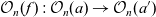
Notation 24. Given a GB-signature ![]() and
and
 $o\in\mathcal{O}_{n}(a)$
, we write
$o\in\mathcal{O}_{n}(a)$
, we write
 $\overline{o}_{j}$
for
$\overline{o}_{j}$
for
 $\alpha_{n,j}(o)$
and
$\alpha_{n,j}(o)$
and
 $\alpha_{o}$
for the tuple
$\alpha_{o}$
for the tuple
 $(\overline{o}_{1},\dots,\overline{o}_{n})$
.
$(\overline{o}_{1},\dots,\overline{o}_{n})$
.
We now introduce our conditions for the generic unification algorithm to be correct.
Definition 25. A GB-signature ![]() is said to be pattern-friendly if
is said to be pattern-friendly if
-
1.
$\mathcal{A}$
has finite connected limits (or equivalently,
$\mathcal{A}$
has pullbacks and equalisers); -
2. all morphisms in
$\mathcal{A}$
are monomorphic; -
3. each
$\mathcal{O}_{n}(-):\mathcal{A}\rightarrow\mathrm{Set}$
preserves finite connected limits; -
4. each
$\alpha_{n,i}$
preserves finite connected limits.


Remark 26. As a counter-example to the third condition, take
 $\mathcal{A}$
to be the category
$\mathcal{A}$
to be the category
 $a\xrightarrow{f}b$
consisting of two objects and one non-identity morphism between them, and consider the syntax generated by two nullary operations in scope a and one nullary operation
$a\xrightarrow{f}b$
consisting of two objects and one non-identity morphism between them, and consider the syntax generated by two nullary operations in scope a and one nullary operation
 $*$
in scope b. The first two conditions of Definition 25 are met, and the fourth one vacuously holds. The third condition is not satisfied for
$*$
in scope b. The first two conditions of Definition 25 are met, and the fourth one vacuously holds. The third condition is not satisfied for
 $n=0$
and the following pullback, essentially because
$n=0$
and the following pullback, essentially because
 $\mathcal{O}_{0}(f)$
is not injective.
$\mathcal{O}_{0}(f)$
is not injective.

Note that
 $M(f)\stackrel{?}{=}*$
has two unifiers given by the two operations in scope a, but none of them factors the other and so there is no most general unifier.
$M(f)\stackrel{?}{=}*$
has two unifiers given by the two operations in scope a, but none of them factors the other and so there is no most general unifier.
These conditions ensure the following two properties.
Property 27 (proved in Section 3.3.1). The following properties hold for pattern-friendly signatures.
-
(i) The action of
$\mathcal{O}_{n}:\mathcal{A}\rightarrow\mathrm{Set}$
on any renaming is an injection: given any
$o\in\mathcal{O}_{n}(b)$
and renaming
$f:a\rightarrow b$
, there is at most one
$o'\in\mathcal{O}_{n}(a)$
such that
$o=o'\{f\}$
. -
(ii) Let
$\mathcal{L}$
be the functor
$\mathcal{A}^{op}\xrightarrow{}\mathrm{MCon}(S)_{\bot}$
mapping a morphism
$x\in\hom_{\mathcal{A}}(b,a)$
to the substitution from
$(X:a)$
to
$(X:b)$
consisting of the single term X(x). Then,
$\mathcal{L}$
preserves finite connected colimits: it maps pullbacks and equalisers in
$\mathcal{A}$
to pushouts and coequalisers in
$\mathrm{MCon}(S)_{\bot}$
.


The first property is used for soundness of the rules ![]() and
and ![]() . It is not satisfied in the counter-example of Remark 26. The second one is used to justify unification of two metavariables applications as pullbacks and equalisers in
. It is not satisfied in the counter-example of Remark 26. The second one is used to justify unification of two metavariables applications as pullbacks and equalisers in
 $\mathcal{A}$
, in the rules
$\mathcal{A}$
, in the rules ![]() and
and ![]() .
.
Lemma 28. A metavariable application
 $\boldsymbol{\Gamma};a\vdash M(x)$
corresponds to the composition
$\boldsymbol{\Gamma};a\vdash M(x)$
corresponds to the composition
 $\mathcal{L}x[in_{M}]$
as a substitution from
$\mathcal{L}x[in_{M}]$
as a substitution from
 $X:a$
to
$X:a$
to
 $\boldsymbol{\Gamma}$
, where
$\boldsymbol{\Gamma}$
, where
 $in_{M}$
is the coproduct injection
$in_{M}$
is the coproduct injection
 $(X:m)\xrightarrow{\cong}(M:m)\hookrightarrow\boldsymbol{\Gamma}$
mapping M to
$(X:m)\xrightarrow{\cong}(M:m)\hookrightarrow\boldsymbol{\Gamma}$
mapping M to
 $M(1_{m})$
.
$M(1_{m})$
.
In the rest of this section, we provide Initial Algebra Semantics for the generated syntax (this is used in the proof of Assumption 27.(ii)).
Any GB-signature ![]() , generates an endofunctor
, generates an endofunctor
 $F_{S}$
on
$F_{S}$
on
 $[\mathcal{A},\mathrm{Set}]$
, that we denote by just F when the context is clear, defined by
$[\mathcal{A},\mathrm{Set}]$
, that we denote by just F when the context is clear, defined by
 \[F_{S}(X)_{a}=\coprod_{n\in\mathbb{N}}\coprod_{o\in\mathcal{O}_{n}(a)}X_{\overline{o}_{1}}\times\dots\times X_{\overline{o}_{n}}.\]
Lemma 29 (proved in Section 3.3.2). F is finitary and generates a free monad T. Moreover, TX is the initial algebra of
 $Z\mapsto X+FZ$
.
$Z\mapsto X+FZ$
.
Lemma 30. The proper syntax generated by a GB-signature (see Figure 7) is recovered as free algebras for F. More precisely, given a metacontext
 $\boldsymbol{\Gamma}=(M_{1}:m_{1},\dots,M_{p}:m_{p})$
,
$\boldsymbol{\Gamma}=(M_{1}:m_{1},\dots,M_{p}:m_{p})$
,
 \[T(\underline{\Gamma})_{a}\cong\{t\ |\ \Gamma;a\vdash t\}\]
where
 $\underline{\boldsymbol{\Gamma}}:\mathcal{A}\rightarrow\mathrm{Set}$
is defined as the coproduct of representable functors mapping a to
$\underline{\boldsymbol{\Gamma}}:\mathcal{A}\rightarrow\mathrm{Set}$
is defined as the coproduct of representable functors mapping a to
 $\coprod_{i}\hom_{\mathcal{A}}(m_{i},a)$
. Moreover, the action of
$\coprod_{i}\hom_{\mathcal{A}}(m_{i},a)$
. Moreover, the action of
 $T(\underline{\boldsymbol{\Gamma}})$
on morphisms of
$T(\underline{\boldsymbol{\Gamma}})$
on morphisms of
 $\mathcal{A}$
correspond to renaming.
$\mathcal{A}$
correspond to renaming.
Notation 31. Given a proper metacontext
 $\boldsymbol{\Gamma}$
. We sometimes denote
$\boldsymbol{\Gamma}$
. We sometimes denote
 $\underline{\boldsymbol{\Gamma}}$
just by
$\underline{\boldsymbol{\Gamma}}$
just by
 $\boldsymbol{\Gamma}$
.
$\boldsymbol{\Gamma}$
.
If
 $\boldsymbol{\Gamma}=(M_{1}:m_{1},...,M_{p}:m_{p})$
and
$\boldsymbol{\Gamma}=(M_{1}:m_{1},...,M_{p}:m_{p})$
and
 $\boldsymbol{\Delta}$
are metacontexts, a Kleisli morphism
$\boldsymbol{\Delta}$
are metacontexts, a Kleisli morphism
 $\sigma:\boldsymbol{\Gamma}\rightarrow T\boldsymbol{\Delta}$
is equivalently given (by combining the above lemma, the Yoneda Lemma, and the universal property of coproducts) by a metavariable substitution from
$\sigma:\boldsymbol{\Gamma}\rightarrow T\boldsymbol{\Delta}$
is equivalently given (by combining the above lemma, the Yoneda Lemma, and the universal property of coproducts) by a metavariable substitution from
 $\boldsymbol{\Gamma}$
to
$\boldsymbol{\Gamma}$
to
 $\boldsymbol{\Delta}$
. Moreover, Kleisli composition corresponds to composition of substitutions. This provides a formal link between the category of metacontexts
$\boldsymbol{\Delta}$
. Moreover, Kleisli composition corresponds to composition of substitutions. This provides a formal link between the category of metacontexts
 $\mathrm{MCon}(S)$
and the Kleisli category of T (see Section for a definition of the latter category).
$\mathrm{MCon}(S)$
and the Kleisli category of T (see Section for a definition of the latter category).
Notation 32. We denote the Kleisli category of a monad T on
 $\mathscr{B}$
by
$\mathscr{B}$
by
 $Kl_{T}$
: the objects are the same as those of
$Kl_{T}$
: the objects are the same as those of
 $\mathscr{B}$
, and a Kleisli morphism from A to B is a morphism
$\mathscr{B}$
, and a Kleisli morphism from A to B is a morphism
 $A\rightarrow TB$
in
$A\rightarrow TB$
in
 $\mathscr{B}$
. We denote the Kleisli composition of
$\mathscr{B}$
. We denote the Kleisli composition of
 $f:A\rightarrow TB$
and
$f:A\rightarrow TB$
and
 $g:B\rightarrow TC$
by
$g:B\rightarrow TC$
by
 $f[g]:A\rightarrow TC$
.
$f[g]:A\rightarrow TC$
.
Proposition 33 The category
 $\mathrm{MCon}(S)$
is equivalent to the full subcategory of
$\mathrm{MCon}(S)$
is equivalent to the full subcategory of
 $Kl_{T}$
spanned by coproducts of representable functors.
$Kl_{T}$
spanned by coproducts of representable functors.
Remark 34. It follows from Proposition 33 and (Mac Lane, 1998, Exercise VI.5.1) that
 $\mathrm{MCon}(S)$
fully faithfully embeds in the category of algebras of T, by mapping a metacontext
$\mathrm{MCon}(S)$
fully faithfully embeds in the category of algebras of T, by mapping a metacontext
 $\boldsymbol{\Gamma}$
to the free algebra
$\boldsymbol{\Gamma}$
to the free algebra
 $T\boldsymbol{\Gamma}$
. In fact,
$T\boldsymbol{\Gamma}$
. In fact,
 $\mathrm{MCon}(S)_{\bot}$
also fully faithfully embeds in the category of algebras by mapping
$\mathrm{MCon}(S)_{\bot}$
also fully faithfully embeds in the category of algebras by mapping
 $\bot$
to the terminal algebra, whose underlying functor maps any object of
$\bot$
to the terminal algebra, whose underlying functor maps any object of
 $\mathcal{A}$
to a singleton set.
$\mathcal{A}$
to a singleton set.
We exploit this characterisation to prove various properties of this category when the signature is pattern-friendly.
Notation 35. Given a GB-signature ![]() , we denote the full subcategory of
, we denote the full subcategory of
 $[\mathcal{A},\mathrm{Set}]$
consisting of functors preserving finite connected limits by
$[\mathcal{A},\mathrm{Set}]$
consisting of functors preserving finite connected limits by
 $\mathscr{C}_{S}$
, or sometimes by
$\mathscr{C}_{S}$
, or sometimes by
 $\mathscr{C}$
, leaving S implicit.
$\mathscr{C}$
, leaving S implicit.
Lemma 36
(proved in Section 3.3.3). Given a GB-signature ![]() such that
such that
 $\mathcal{A}$
has finite connected limits,
$\mathcal{A}$
has finite connected limits,
 $F_{S}$
restricts as an endofunctor on
$F_{S}$
restricts as an endofunctor on
 $\mathscr{C}_{S}$
if and only if the last two conditions of Definition 25 hold.
$\mathscr{C}_{S}$
if and only if the last two conditions of Definition 25 hold.
We now assume given a pattern-friendly signature ![]() .
.
Lemma 37 (proved in Section 3.3.4).
 $\mathscr{C}$
is closed under limits, coproducts, and filtered colimits. Moreover, it is cocomplete.
$\mathscr{C}$
is closed under limits, coproducts, and filtered colimits. Moreover, it is cocomplete.
Corollary 38 (proved in Section 3.3.5). T restricts as a monad on
 $\mathscr{C}$
freely generated by the restriction of F as an endofunctor on
$\mathscr{C}$
freely generated by the restriction of F as an endofunctor on
 $\mathscr{C}$
(Lemma 36).
$\mathscr{C}$
(Lemma 36).
3.3 Proofs of statements in Section 3.2
3.3.1 Property 27
We use the notations and definitions of Section 3.2.
Let us first prove the first item.
Proof of Property 27.(i) We show that given any
 $o\in\mathcal{O}_{n}(b)$
and renaming
$o\in\mathcal{O}_{n}(b)$
and renaming
 $f:a\rightarrow b$
, there is at most one
$f:a\rightarrow b$
, there is at most one
 $o'\in\mathcal{O}_{n}(a)$
such that
$o'\in\mathcal{O}_{n}(a)$
such that
 $o=o'\{f\}$
.
$o=o'\{f\}$
.
Note that a morphism
 $f:a\rightarrow b$
is monomorphic if and only if the following square is a pullback (Mac Lane, Reference Mac Lane1998, Exercise III.4.4), as shown by unfolding the universal property of this particular limit.
$f:a\rightarrow b$
is monomorphic if and only if the following square is a pullback (Mac Lane, Reference Mac Lane1998, Exercise III.4.4), as shown by unfolding the universal property of this particular limit.

Therefore, since
 $\mathcal{O}_{n}$
preserves finite connected limits, it also preserves monomorphisms.
$\mathcal{O}_{n}$
preserves finite connected limits, it also preserves monomorphisms.
The rest of this section is devoted to the proof of Property 27.(ii).
By right continuity of the homset bifunctor, any representable functor is in
 $\mathscr{C}$
and thus the embedding
$\mathscr{C}$
and thus the embedding
 $\mathscr{C}\rightarrow[\mathcal{A},\mathrm{Set}]$
factors the Yoneda embedding
$\mathscr{C}\rightarrow[\mathcal{A},\mathrm{Set}]$
factors the Yoneda embedding
 $\mathcal{A}^{op}\rightarrow[\mathcal{A},\mathrm{Set}]$
.
$\mathcal{A}^{op}\rightarrow[\mathcal{A},\mathrm{Set}]$
.
Lemma 39. Let
 $\mathscr{D}$
denote the opposite category of
$\mathscr{D}$
denote the opposite category of
 $\mathcal{A}$
and
$\mathcal{A}$
and
 $K:\mathscr{D}\rightarrow\mathscr{C}$
the factorisation of
$K:\mathscr{D}\rightarrow\mathscr{C}$
the factorisation of
 $\mathscr{C}\rightarrow[\mathcal{A},\mathrm{Set}]$
by the Yoneda embedding. Then,
$\mathscr{C}\rightarrow[\mathcal{A},\mathrm{Set}]$
by the Yoneda embedding. Then,
 $K:\mathscr{D}\rightarrow\mathscr{C}$
preserves finite connected colimits.
$K:\mathscr{D}\rightarrow\mathscr{C}$
preserves finite connected colimits.
Proof This essentially follows from the fact functors in
 $\mathscr{C}$
preserves finite connected limits. Let us detail the argument: let
$\mathscr{C}$
preserves finite connected limits. Let us detail the argument: let
 $y:\mathcal{A}^{op}\rightarrow[\mathcal{A},\mathrm{Set}]$
denote the Yoneda embedding and
$y:\mathcal{A}^{op}\rightarrow[\mathcal{A},\mathrm{Set}]$
denote the Yoneda embedding and
 $J:\mathscr{C}\rightarrow[\mathcal{A},\mathrm{Set}]$
denote the canonical embedding, so that
$J:\mathscr{C}\rightarrow[\mathcal{A},\mathrm{Set}]$
denote the canonical embedding, so that
 \begin{equation}y=J\circ K.\end{equation}
Now consider a finite connected limit
 $\lim F$
in
$\lim F$
in
 $\mathcal{A}$
. Then,
$\mathcal{A}$
. Then,

These isomorphisms are natural in X and thus
 $K\lim F\cong\mathrm{colim}\ KF$
.
$K\lim F\cong\mathrm{colim}\ KF$
.
Proof
of Assumption 27.(ii) Note that
 $\mathcal{L}$
factors as
$\mathcal{L}$
factors as
 \[\mathscr{D}\xrightarrow{\mathcal{L}^{\bullet}}\mathrm{MCon}(S)\hookrightarrow\mathrm{MCon}(S)_{\bot},\]
where the right embedding preserves colimits by Lemma 17.(i), so it is enough to show that
 $\mathcal{L}^{\bullet}$
preserves finite connected colimits. Let
$\mathcal{L}^{\bullet}$
preserves finite connected colimits. Let
 $T_{|\mathscr{C}}$
be the monad T restricted to
$T_{|\mathscr{C}}$
be the monad T restricted to
 $\mathscr{C}$
, following Corollary 38. Since
$\mathscr{C}$
, following Corollary 38. Since
 $K:\mathscr{D}\rightarrow\mathscr{C}$
preserves finite connected colimits (Lemma 39), composing it with the left adjoint
$K:\mathscr{D}\rightarrow\mathscr{C}$
preserves finite connected colimits (Lemma 39), composing it with the left adjoint
 $\mathscr{C}\rightarrow Kl_{T_{|\mathscr{C}}}$
yields a functor
$\mathscr{C}\rightarrow Kl_{T_{|\mathscr{C}}}$
yields a functor
 $\mathscr{D}\rightarrow Kl_{T_{|\mathscr{C}}}$
also preserving those colimits. Since it factors as
$\mathscr{D}\rightarrow Kl_{T_{|\mathscr{C}}}$
also preserving those colimits. Since it factors as
 $\mathscr{D}\xrightarrow{\mathcal{L}^{\bullet}}\mathrm{MCon}(S)\hookrightarrow Kl_{T_{|\mathscr{C}}}$
, where the right functor is full and faithful,
$\mathscr{D}\xrightarrow{\mathcal{L}^{\bullet}}\mathrm{MCon}(S)\hookrightarrow Kl_{T_{|\mathscr{C}}}$
, where the right functor is full and faithful,
 $\mathcal{L}^{\bullet}$
also preserves finite connected colimits.
$\mathcal{L}^{\bullet}$
also preserves finite connected colimits.
3.3.2 Lemma 29
F is finitary because filtered colimits commute with finite limits (Mac Lane, Reference Mac Lane1998, Theorem IX.2.1) and colimits. The free monad construction is due to Reiterman (Reference Reiterman1977).
3.3.3 Lemma 36
Notation 40. Given a functor
 $F:I\rightarrow\mathscr{B}$
, we denote the limit (resp. colimit) of F by
$F:I\rightarrow\mathscr{B}$
, we denote the limit (resp. colimit) of F by
 $\int_{i:I}F(i)$
or
$\int_{i:I}F(i)$
or
 $\lim F$
(resp.
$\lim F$
(resp.
 $\int^{i:I}F(i)$
or
$\int^{i:I}F(i)$
or
 $\mathrm{colim}\ F$
) and the canonical projection
$\mathrm{colim}\ F$
) and the canonical projection
 $\lim F\rightarrow Fi$
by
$\lim F\rightarrow Fi$
by
 $p_{i}$
for any object i of I.
$p_{i}$
for any object i of I.
This section is dedicated to the proof of the following lemma.
Lemma 41. Given a GB-signature ![]() such that
such that
 $\mathcal{A}$
has finite connected limits,
$\mathcal{A}$
has finite connected limits,
 $F_{S}$
restricts as an endofunctor on the full subcategory
$F_{S}$
restricts as an endofunctor on the full subcategory
 $\mathscr{C}$
of
$\mathscr{C}$
of
 $[\mathcal{A},\mathrm{Set}]$
consisting of functors preserving finite connected limits if and only if each
$[\mathcal{A},\mathrm{Set}]$
consisting of functors preserving finite connected limits if and only if each
 $\mathcal{O}_{n}\in\mathscr{C}$
, and
$\mathcal{O}_{n}\in\mathscr{C}$
, and
 $\alpha_{n,i}:\int\mathcal{O}_{n}\rightarrow\mathcal{A}$
preserves finite connected limits.
$\alpha_{n,i}:\int\mathcal{O}_{n}\rightarrow\mathcal{A}$
preserves finite connected limits.
We first introduce a bunch of intermediate lemmas.
Lemma 42. Let
 $F:\mathscr{B}\rightarrow\mathrm{Set}$
be a functor. For any functor
$F:\mathscr{B}\rightarrow\mathrm{Set}$
be a functor. For any functor
 $G:I\rightarrow\int F$
, denoting by H the composite functor
$G:I\rightarrow\int F$
, denoting by H the composite functor
 $I\xrightarrow{G}\int F\rightarrow\mathscr{B}$
, there exists a unique
$I\xrightarrow{G}\int F\rightarrow\mathscr{B}$
, there exists a unique
 $x\in\lim(F\circ H)$
such that
$x\in\lim(F\circ H)$
such that
 $Gi=(Hi,p_{i}(x))$
.
$Gi=(Hi,p_{i}(x))$
.
Proof
 $\int F$
is isomorphic to the opposite of the comma category
$\int F$
is isomorphic to the opposite of the comma category
 $y/F$
, where
$y/F$
, where
 $y:\mathscr{B}^{op}\rightarrow[\mathscr{B},\mathrm{Set}]$
is the Yoneda embedding. The statement follows from the universal property of a comma category.
$y:\mathscr{B}^{op}\rightarrow[\mathscr{B},\mathrm{Set}]$
is the Yoneda embedding. The statement follows from the universal property of a comma category.
Lemma 43. Let
 $F:\mathscr{B}\rightarrow\mathrm{Set}$
and
$F:\mathscr{B}\rightarrow\mathrm{Set}$
and
 $G:I\rightarrow\int F$
such that F preserves the limit of
$G:I\rightarrow\int F$
such that F preserves the limit of
 $H:I\xrightarrow{G}\int F\xrightarrow{}\mathscr{B}$
. Then, there exists a unique
$H:I\xrightarrow{G}\int F\xrightarrow{}\mathscr{B}$
. Then, there exists a unique
 $x\in F\lim H$
such that
$x\in F\lim H$
such that
 $Gi=(Hi,Fp_{i}(x))$
and moreover,
$Gi=(Hi,Fp_{i}(x))$
and moreover,
 $(\lim H,x)$
is the limit of G.
$(\lim H,x)$
is the limit of G.
Proof The unique existence of
 $x\in F\lim H$
such that
$x\in F\lim H$
such that
 $Gi=(Hi,Fp_{i}(x))$
follows from Lemma 42 and the fact that F preserves
$Gi=(Hi,Fp_{i}(x))$
follows from Lemma 42 and the fact that F preserves
 $\lim H$
. Let
$\lim H$
. Let
 $\mathscr{C}$
denote the full subcategory of
$\mathscr{C}$
denote the full subcategory of
 $[\mathscr{B},\mathrm{Set}]$
of functors preserving
$[\mathscr{B},\mathrm{Set}]$
of functors preserving
 $\lim G$
. Note that
$\lim G$
. Note that
 $\int F$
is isomorphic to the opposite of the comma category
$\int F$
is isomorphic to the opposite of the comma category
 $K/F$
, where
$K/F$
, where
 $K:\mathscr{B}^{op}\rightarrow\mathscr{C}$
is the Yoneda embedding, which preserves
$K:\mathscr{B}^{op}\rightarrow\mathscr{C}$
is the Yoneda embedding, which preserves
 $\mathrm{colim}\ G$
, by an argument similar to the proof of Lemma 39. We conclude from the fact that the forgetful functor from a comma category
$\mathrm{colim}\ G$
, by an argument similar to the proof of Lemma 39. We conclude from the fact that the forgetful functor from a comma category
 $L/R$
to the product of the categories creates colimits that L preserve.
$L/R$
to the product of the categories creates colimits that L preserve.
Corollary 44. Let I be a small category,
 $\mathscr{B}$
and
$\mathscr{B}$
and
 $\mathscr{B}'$
be categories with I-limits (i.e., limits of any diagram over I). Let
$\mathscr{B}'$
be categories with I-limits (i.e., limits of any diagram over I). Let
 $F:\mathscr{B}\rightarrow\mathrm{Set}$
be a functor preserving those limits. Then,
$F:\mathscr{B}\rightarrow\mathrm{Set}$
be a functor preserving those limits. Then,
 $\int F$
has I-limits, preserved by the projection
$\int F$
has I-limits, preserved by the projection
 $\int F\rightarrow\mathscr{B}$
. Moreover, a functor
$\int F\rightarrow\mathscr{B}$
. Moreover, a functor
 $G:\int F\rightarrow\mathscr{B}'$
preserves them if and only if for any
$G:\int F\rightarrow\mathscr{B}'$
preserves them if and only if for any
 $d:I\rightarrow\mathscr{B}$
and
$d:I\rightarrow\mathscr{B}$
and
 $x\in F\lim d$
, the canonical morphism
$x\in F\lim d$
, the canonical morphism
 $G(\lim d,x)\rightarrow\int_{i:I}G(d_{i},Fp_{i}(x))$
is an isomorphism.
$G(\lim d,x)\rightarrow\int_{i:I}G(d_{i},Fp_{i}(x))$
is an isomorphism.
Proof By Lemma 43, a diagram
 $d':I\rightarrow\int F$
is equivalently given by
$d':I\rightarrow\int F$
is equivalently given by
 $d:I\rightarrow\mathscr{B}$
and
$d:I\rightarrow\mathscr{B}$
and
 $x\in F\lim d$
, recovering d’ as
$x\in F\lim d$
, recovering d’ as
 $d'_{i}=(d_{i},Fp_{i}(x))$
, and moreover
$d'_{i}=(d_{i},Fp_{i}(x))$
, and moreover
 $\lim d'=(\lim d,x)$
.
$\lim d'=(\lim d,x)$
.
Corollary 45. Assuming that
 $\mathcal{A}$
has finite connected limits and each
$\mathcal{A}$
has finite connected limits and each
 $\mathcal{O}_{n}$
preserves finite connected limits, the finite limit preservation on
$\mathcal{O}_{n}$
preserves finite connected limits, the finite limit preservation on
 $\alpha:\int J\rightarrow\mathcal{A}$
of Lemma 41 can be reformulated as follows: given a finite connected diagram
$\alpha:\int J\rightarrow\mathcal{A}$
of Lemma 41 can be reformulated as follows: given a finite connected diagram
 $d:D\rightarrow\mathcal{A}$
and element
$d:D\rightarrow\mathcal{A}$
and element
 $o\in\mathcal{O}_{n}(\lim d)$
, the following canonical morphism is an isomorphism
$o\in\mathcal{O}_{n}(\lim d)$
, the following canonical morphism is an isomorphism
 \[\overline{o}_{j}\rightarrow\int_{i:D}\overline{o\{p_{i}\}}_{j}\]
for any
 $j\in\{1,\dots,n\}$
.
$j\in\{1,\dots,n\}$
.
Proof Note that, by definition,
 $\overline{o}_{j}=\alpha_{n,j}(\lim d,o)$
, and
$\overline{o}_{j}=\alpha_{n,j}(\lim d,o)$
, and
 $\overline{o\{p_{i}\}}_{j}=\alpha_{n,j}(d_{i},o\{p_{i}\})$
. This is a direct application of Corollary 44.
$\overline{o\{p_{i}\}}_{j}=\alpha_{n,j}(d_{i},o\{p_{i}\})$
. This is a direct application of Corollary 44.
Lemma 46 (Limits commute with dependent pairs). Given functors
 $K:I\rightarrow\mathrm{Set}$
and
$K:I\rightarrow\mathrm{Set}$
and
 $G:\int K\rightarrow\mathrm{Set}$
, the following canonical morphism is an isomorphism
$G:\int K\rightarrow\mathrm{Set}$
, the following canonical morphism is an isomorphism
 \[\coprod_{\alpha\in\lim K}\int_{i:I}G(i,p_{i}(\alpha))\rightarrow\int_{i:I}\coprod_{x\in Ki}G(i,x)\]
Proof The domain consists of a family
 $(\alpha_{i})_{i\in I}$
where
$(\alpha_{i})_{i\in I}$
where
 $\alpha_{i}\in K_{i}$
together with a family
$\alpha_{i}\in K_{i}$
together with a family
 $(g_{i})_{i\in I}$
where
$(g_{i})_{i\in I}$
where
 $g_{i}\in G(i,\alpha_{i})$
, such that that for each morphism
$g_{i}\in G(i,\alpha_{i})$
, such that that for each morphism
 $i\xrightarrow{u}j$
in I, we have
$i\xrightarrow{u}j$
in I, we have
 $Ku(\alpha_{i})=\alpha_{j}$
and
$Ku(\alpha_{i})=\alpha_{j}$
and
 $(Gu)(g_{i})=g_{j}$
.
$(Gu)(g_{i})=g_{j}$
.
The codomain consists of a family
 $(x_{i},g_{i})_{i\in I}$
where
$(x_{i},g_{i})_{i\in I}$
where
 $x_{i}\in Ki$
and
$x_{i}\in Ki$
and
 $g_{i}\in G(i,x_{i})$
, such that for each morphism
$g_{i}\in G(i,x_{i})$
, such that for each morphism
 $i\xrightarrow{u}j$
in I, we have
$i\xrightarrow{u}j$
in I, we have
 $Ku(x_{i})=x_{j}$
and
$Ku(x_{i})=x_{j}$
and
 $(Gu)(g_{i})=g_{j}$
.
$(Gu)(g_{i})=g_{j}$
.
The canonical morphism maps
 $((x_{i})_{i\in I},(g_{i})_{i\in I})$
to the family
$((x_{i})_{i\in I},(g_{i})_{i\in I})$
to the family
 $(x_{i},g_{i})_{i\in I}$
. It is clearly a bijection.
$(x_{i},g_{i})_{i\in I}$
. It is clearly a bijection.
Lemma 47. A coproduct
 $\coprod_{i}G_{i}$
of functors from a small category
$\coprod_{i}G_{i}$
of functors from a small category
 $\mathcal{B}$
with finite connected limits to Set preserves those limits if and only if each
$\mathcal{B}$
with finite connected limits to Set preserves those limits if and only if each
 $G_{i}$
does.
$G_{i}$
does.
Proof This is a consequence of the following statement, which is a direct application of Adámek et al. (Reference Adámek, Borceux, Lack and Rosicky2002, Theorem 2.4 and Example 2.3.(iii)): if
 $\mathscr{B}$
is a small category with finite connected limits, then a functor
$\mathscr{B}$
is a small category with finite connected limits, then a functor
 $G:\mathscr{B}\rightarrow\mathrm{Set}$
preserves those limits if and only if
$G:\mathscr{B}\rightarrow\mathrm{Set}$
preserves those limits if and only if
 $\int G$
is a coproduct of filtered categories.
$\int G$
is a coproduct of filtered categories.
Proof
of Lemma 41 Let
 $d:I\rightarrow\mathcal{A}$
be a finite connected diagram and X be a functor preserving finite connected limits. Then,
$d:I\rightarrow\mathcal{A}$
be a finite connected diagram and X be a functor preserving finite connected limits. Then,

Thus, since X preserves finite connected limits by assumption,
 \begin{align}\int_{i}F(X)_{d_{i}} & =\coprod_{n}\coprod_{o\in\int_{i}\mathcal{O}_{n}(d_{i})}X_{\int_{i:I}\overline{p_{i}(o)}_{1}}\times\dots\times X_{\int_{i:I}\overline{p_{i}(o)}_{n}}\end{align}
Now, let us prove the only if statement first. Assume that each
 $\mathcal{O}_{n}$
and
$\mathcal{O}_{n}$
and
 $\alpha_{n,i}:\int\mathcal{O}_{n}\rightarrow\mathcal{A}$
preserve finite connected limits. Then,
$\alpha_{n,i}:\int\mathcal{O}_{n}\rightarrow\mathcal{A}$
preserve finite connected limits. Then,

Conversely, let us assume that F restricts to an endofunctor on
 $\mathscr{C}$
. Then,
$\mathscr{C}$
. Then,
 $F(1)=\coprod_{n}\mathcal{O}_{n}$
preserves finite connected limits. By Lemma 47, each
$F(1)=\coprod_{n}\mathcal{O}_{n}$
preserves finite connected limits. By Lemma 47, each
 $\mathcal{O}_{n}$
preserves finite connected limits. By Corollary 45, it is enough to prove that given a finite connected diagram
$\mathcal{O}_{n}$
preserves finite connected limits. By Corollary 45, it is enough to prove that given a finite connected diagram
 $d:D\rightarrow\mathcal{A}$
and element
$d:D\rightarrow\mathcal{A}$
and element
 $o\in\mathcal{O}_{n}(\lim d)$
, the following canonical morphism is an isomorphism
$o\in\mathcal{O}_{n}(\lim d)$
, the following canonical morphism is an isomorphism
 \[\overline{o}_{j}\rightarrow\int_{i:D}\overline{o\{p_{i}\}}_{j}\]
Now, we have

On the other hand,

It follows from those two chains of isomorphisms that each function
 $X_{\overline{o}_{j}}\rightarrow X_{\int_{i:I}\overline{o\{p_{i}\}}_{j}}$
is a bijection, or equivalently (by the Yoneda Lemma), that
$X_{\overline{o}_{j}}\rightarrow X_{\int_{i:I}\overline{o\{p_{i}\}}_{j}}$
is a bijection, or equivalently (by the Yoneda Lemma), that
 $\mathscr{C}(K\overline{o}_{j},X)\rightarrow\mathscr{C}(K\int_{i:I}\overline{o\{p_{i}\}}_{j},X)$
is an isomorphism. Since the Yoneda embedding is fully faithful,
$\mathscr{C}(K\overline{o}_{j},X)\rightarrow\mathscr{C}(K\int_{i:I}\overline{o\{p_{i}\}}_{j},X)$
is an isomorphism. Since the Yoneda embedding is fully faithful,
 $\overline{o}_{j}\rightarrow\int_{i:D}\overline{o\{p_{i}\}}_{j}$
is an isomorphism.
$\overline{o}_{j}\rightarrow\int_{i:D}\overline{o\{p_{i}\}}_{j}$
is an isomorphism.
3.3.4 Lemma 37
Cocompleteness follows from Adámek & Rosicky, (Reference Adámek and Rosicky1994, Remark 1.56), since
 $\mathscr{C}$
is the category of models of a limit sketch, and is thus locally presentable, by Adámek & Rosicky (Reference Adámek and Rosicky1994, Proposition 1.51).
$\mathscr{C}$
is the category of models of a limit sketch, and is thus locally presentable, by Adámek & Rosicky (Reference Adámek and Rosicky1994, Proposition 1.51).
For the claimed closure property, all we have to check is that limits, coproducts, and filtered colimits of functors preserving finite connected limits still preserve finite connected limits. The case of limits is clear, since limits commute with limits. Coproducts and filtered colimits also commute with finite connected limits (Adámek et al., Reference Adámek, Borceux, Lack and Rosicky2002, Example 1.3.(vi)).
3.3.5 Corollary 38
The result follows from the construction of T using colimits of initial chains, thanks to the closure properties of
 $\mathscr{C}$
. More specifically, TX can be constructed as the colimit of the chain
$\mathscr{C}$
. More specifically, TX can be constructed as the colimit of the chain
 $\emptyset\rightarrow H\emptyset\rightarrow HH\emptyset\rightarrow\dots$
, where
$\emptyset\rightarrow H\emptyset\rightarrow HH\emptyset\rightarrow\dots$
, where
 $\emptyset$
denotes the constant functor mapping anything to the empty set, and
$\emptyset$
denotes the constant functor mapping anything to the empty set, and
 $HZ=FZ+X$
.
$HZ=FZ+X$
.
4 Soundness of the pruning phase
In this section, we assume a pattern-friendly GB-signature S and discuss soundness of the main rules of the two mutually recursive functions ![]() and
and ![]() listed in Figure 10, which handle unification of two substitutions
listed in Figure 10, which handle unification of two substitutions
 $\delta:\boldsymbol{\Gamma'_{1}}\rightarrow\Gamma$
and
$\delta:\boldsymbol{\Gamma'_{1}}\rightarrow\Gamma$
and
 $\overline{x}:\boldsymbol{\Gamma'_{1}}\rightarrow\boldsymbol{\Gamma'_{2}}$
where
$\overline{x}:\boldsymbol{\Gamma'_{1}}\rightarrow\boldsymbol{\Gamma'_{2}}$
where
 $\overline{x}$
is induced by a vector
$\overline{x}$
is induced by a vector
 $x:\boldsymbol{\Gamma'_{2}}\dashrightarrow\boldsymbol{\Gamma'_{1}}$
of renamings (Definition 8). Strictly speaking, this is not unification as we introduced it because
$x:\boldsymbol{\Gamma'_{2}}\dashrightarrow\boldsymbol{\Gamma'_{1}}$
of renamings (Definition 8). Strictly speaking, this is not unification as we introduced it because
 $\delta$
and
$\delta$
and
 $\overline{x}$
do not target the same context, but it is straightforward to adapt the definition: a unifier is given by two substitutions
$\overline{x}$
do not target the same context, but it is straightforward to adapt the definition: a unifier is given by two substitutions
 $\sigma:\Gamma\rightarrow\Delta$
and
$\sigma:\Gamma\rightarrow\Delta$
and
 $\sigma':\boldsymbol{\Gamma'_{2}}\rightarrow\Delta$
such that the following equation holds
$\sigma':\boldsymbol{\Gamma'_{2}}\rightarrow\Delta$
such that the following equation holds
 \begin{equation}\delta[\sigma]=\overline{x}[\sigma']\end{equation}
As usual, the mgu is defined as the unifier uniquely factoring any other unifier.
Lemma 48. The right-hand side
 $\overline{x}[\sigma']$
in (4.1) is actually equal to
$\overline{x}[\sigma']$
in (4.1) is actually equal to
 $\sigma'\{x\}$
. Indeed,
$\sigma'\{x\}$
. Indeed,
 $\overline{x}=(\dots,M_{i}(x_{i}),\dots)$
and
$\overline{x}=(\dots,M_{i}(x_{i}),\dots)$
and
 $M_{i}(x_{i})[\sigma']=\sigma'_{i}\{x_{i}\}$
.
$M_{i}(x_{i})[\sigma']=\sigma'_{i}\{x_{i}\}$
.
From a categorical point of view, such a mgu is characterised as a pushout.
Notation 49. Given
•
 $\delta:\boldsymbol{\Gamma'_{1}}\rightarrow\Gamma$
,
$\delta:\boldsymbol{\Gamma'_{1}}\rightarrow\Gamma$
,
•
 $x:\boldsymbol{\Gamma'_{2}}\dashrightarrow\boldsymbol{\Gamma'_{1}}$
,
$x:\boldsymbol{\Gamma'_{2}}\dashrightarrow\boldsymbol{\Gamma'_{1}}$
,
•
 $\sigma:\Gamma\rightarrow\Delta$
,
$\sigma:\Gamma\rightarrow\Delta$
,
•
 $\sigma':\boldsymbol{\Gamma'_{2}}\rightarrow\Delta$
,
$\sigma':\boldsymbol{\Gamma'_{2}}\rightarrow\Delta$
,
the notation
 $\Gamma\vdash_{}\delta\boldsymbol{:>}x\Rightarrow\sigma';\sigma\dashv\Delta$
means that the square
$\Gamma\vdash_{}\delta\boldsymbol{:>}x\Rightarrow\sigma';\sigma\dashv\Delta$
means that the square 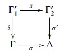 is a pushout in
 $\mathrm{MCon}(S)_{\bot}$
.
$\mathrm{MCon}(S)_{\bot}$
.
Remark 50. This justifies the similarity between the pruning notation
 $-\vdash_{}-\boldsymbol{:>}-\Rightarrow-;-$
and the pullback notation of Notation 9, since pushouts in a category are nothing but pullbacks in the opposite category.
$-\vdash_{}-\boldsymbol{:>}-\Rightarrow-;-$
and the pullback notation of Notation 9, since pushouts in a category are nothing but pullbacks in the opposite category.
In the following subsections, we detail soundness of the rules for the rigid case (Section 4.1) and then for the flex case (Section 4.2).
The rules ![]() and
and ![]() are straightforward adaptions specialised to those specific unification problems of the rules
are straightforward adaptions specialised to those specific unification problems of the rules ![]() and
and ![]() described later in Section 5.1. The failing rule
described later in Section 5.1. The failing rule ![]() is justified by Lemma 17.(ii).
is justified by Lemma 17.(ii).
4.1 Rigid (rules and
The rules ![]() and
and ![]() handle non-cyclic unification of M(x) with
handle non-cyclic unification of M(x) with
 $\boldsymbol{\Gamma};a\vdash o(\delta)$
for some
$\boldsymbol{\Gamma};a\vdash o(\delta)$
for some
 $o\in\mathcal{O}_{n}(a)$
, where
$o\in\mathcal{O}_{n}(a)$
, where
 $M\notin\boldsymbol{\Gamma}$
. By Lemma 48, a unifier is given by a substitution
$M\notin\boldsymbol{\Gamma}$
. By Lemma 48, a unifier is given by a substitution
 $\sigma:\Gamma\rightarrow\Delta$
and a term u such that
$\sigma:\Gamma\rightarrow\Delta$
and a term u such that
 \begin{equation}o(\delta[\sigma])=u\{x\}.\end{equation}
Now, u is either some M(y) or
 $o'(\vec{v})$
. But in the first case,
$o'(\vec{v})$
. But in the first case,
 $u\{x\}=M(y)\{x\}=M(x\circ y)$
, contradicting Equation (4.2). Therefore,
$u\{x\}=M(y)\{x\}=M(x\circ y)$
, contradicting Equation (4.2). Therefore,
 $u=o'(\delta')$
for some
$u=o'(\delta')$
for some
 $o'\in\mathcal{O}_{n}(m)$
and
$o'\in\mathcal{O}_{n}(m)$
and
 $\delta'$
is a substitution from
$\delta'$
is a substitution from
 $\alpha_{o'}$
to
$\alpha_{o'}$
to
 $\Delta$
. Then,
$\Delta$
. Then,
 $u\{x\}=o'\{x\}(\delta\{x_{}^{o'}\})$
. It follows from Equation (4.2) that
$u\{x\}=o'\{x\}(\delta\{x_{}^{o'}\})$
. It follows from Equation (4.2) that
 $o=o'\{x\}$
, and
$o=o'\{x\}$
, and
 $\delta[\sigma]=\delta'\{x_{}^{o'}\}$
.
$\delta[\sigma]=\delta'\{x_{}^{o'}\}$
.
Note that there is at most one o’ such that
 $o=o'\{x\}$
, by Assumption 27.(i). In this case, a unifier is equivalently given by substitutions
$o=o'\{x\}$
, by Assumption 27.(i). In this case, a unifier is equivalently given by substitutions
 $\sigma:\Gamma\rightarrow\Delta$
and
$\sigma:\Gamma\rightarrow\Delta$
and
 $\sigma':\alpha_{o'}\rightarrow\Delta$
such that
$\sigma':\alpha_{o'}\rightarrow\Delta$
such that
 $\delta[\sigma]=\sigma'\{x_{}^{o'}\}$
. But, by Lemma 48, this is precisely the data for a unifier of
$\delta[\sigma]=\sigma'\{x_{}^{o'}\}$
. But, by Lemma 48, this is precisely the data for a unifier of
 $\delta$
and
$\delta$
and
 $x^{o'}$
. This actually induces an isomorphism between the two categories of unifiers, thus justifying the rules
$x^{o'}$
. This actually induces an isomorphism between the two categories of unifiers, thus justifying the rules ![]() and
and ![]() .
.
4.2 Flex (rule )
The rule ![]() handles unification of M(x) with N(y) where
handles unification of M(x) with N(y) where
 $M\neq N$
in a scope a. More explicitly, this is about computing the pushout of
$M\neq N$
in a scope a. More explicitly, this is about computing the pushout of ![]() and
and
 $(X:a)\xrightarrow{\mathcal{L}y}(X:n)\xrightarrow{\cong}(N:n)$
.
$(X:a)\xrightarrow{\mathcal{L}y}(X:n)\xrightarrow{\cong}(N:n)$
.
Thanks to the following lemma, it is actually enough to compute the pushout of
 $\mathcal{L}x$
and
$\mathcal{L}x$
and
 $\mathcal{L}y$
, taking
$\mathcal{L}y$
, taking
 $A=(X:a)$
,
$A=(X:a)$
,
 $B=(X:m)$
,
$B=(X:m)$
,
 $C=(X:n)$
,
$C=(X:n)$
,
 $Y=\boldsymbol{\Gamma}\backslash M$
, so that
$Y=\boldsymbol{\Gamma}\backslash M$
, so that
 $B+Y\cong\boldsymbol{\Gamma}$
, since coproduct is concatenation of metacontext by Corollary 18.
$B+Y\cong\boldsymbol{\Gamma}$
, since coproduct is concatenation of metacontext by Corollary 18.
Lemma 51. In any category, if the square below left is a pushout, then so is the square below right.

By Assumption 27.(ii), the pushout of
 $\mathcal{L}x$
and
$\mathcal{L}x$
and
 $\mathcal{L}y$
is the image by
$\mathcal{L}y$
is the image by
 $\mathcal{L}$
of the pullback of x and y in
$\mathcal{L}$
of the pullback of x and y in
 $\mathcal{A}$
, thus justifying the rule
$\mathcal{A}$
, thus justifying the rule ![]() .
.
5 Soundness of the unification phase
In this section, we assume a pattern-friendly GB-signature S and discuss soundness of the main rules of the two mutually recursive functions ![]() and
and ![]() listed in Figure 10, which compute coequalisers in
listed in Figure 10, which compute coequalisers in
 $\mathrm{MCon}(S)_{\bot}$
.
$\mathrm{MCon}(S)_{\bot}$
.
The failing rules ![]() and
and ![]() are justified by Lemma 17.(ii). Both rules
are justified by Lemma 17.(ii). Both rules ![]() and
and ![]() handle unification of two rigid terms
handle unification of two rigid terms
 $o(\delta)$
and
$o(\delta)$
and
 $o'(\delta')$
. If
$o'(\delta')$
. If
 $o\neq o'$
, they do not have any unifier: this is the rule
$o\neq o'$
, they do not have any unifier: this is the rule ![]() . If
. If
 $o=o'$
, then a substitution is a unifier if and only if it unifies
$o=o'$
, then a substitution is a unifier if and only if it unifies
 $\delta$
and
$\delta$
and
 $\delta'$
, thus justifying the
$\delta'$
, thus justifying the ![]() rule.
rule.
In the next subsections, we discuss the rule sequential rules ![]() and
and ![]() (Section 5.1), the rule
(Section 5.1), the rule ![]() transitioning to the pruning phase (Section 5.2), the rule
transitioning to the pruning phase (Section 5.2), the rule ![]() unifying metavariable with itself (Section 5.3), and the failing rule
unifying metavariable with itself (Section 5.3), and the failing rule ![]() for cyclic unification of a metavariable with a term which includes it deeply (Section 5.4).
for cyclic unification of a metavariable with a term which includes it deeply (Section 5.4).
5.1 Sequential unification (rules and )
The rule ![]() is a direct application of the following general lemma, since the empty metavariable context is initial: the only morphism to any metacontext
is a direct application of the following general lemma, since the empty metavariable context is initial: the only morphism to any metacontext
 $\Gamma$
is the empty metasubstitution ().
$\Gamma$
is the empty metasubstitution ().
Lemma 52. If A is initial in a category, then any diagram of the shape ![]() is a coequaliser.
is a coequaliser.
The rule ![]() is a direct application of a stepwise construction of coequalisers valid in any category, as noted by Rydeheard & Burstall (Reference Rydeheard and Burstall1988, Theorem 9): if the first two diagrams below are coequalisers, then the last one as well.
is a direct application of a stepwise construction of coequalisers valid in any category, as noted by Rydeheard & Burstall (Reference Rydeheard and Burstall1988, Theorem 9): if the first two diagrams below are coequalisers, then the last one as well.

5.2 Flex-Flex, no cycle (rule )
The rule ![]() transitions from unification to pruning. While unification is a coequaliser construction, in Section 4, we explained that pruning is a pushout construction. The rule is justified by the following well-known connection between those two notions.
transitions from unification to pruning. While unification is a coequaliser construction, in Section 4, we explained that pruning is a pushout construction. The rule is justified by the following well-known connection between those two notions.
Lemma 53. Consider a commuting square  in any category. If the coproduct
 $B+C$
of B and C exists, then this is a pushout if and only if
$B+C$
of B and C exists, then this is a pushout if and only if
 $B+C\xrightarrow{f,g}D$
is the coequaliser of
$B+C\xrightarrow{f,g}D$
is the coequaliser of
 $in_{1}\circ u$
and
$in_{1}\circ u$
and
 $in_{2}\circ v$
.
$in_{2}\circ v$
.
We take B to be
 $M:m$
and C to be
$M:m$
and C to be
 $\boldsymbol{\Gamma}\backslash M$
. The premise
$\boldsymbol{\Gamma}\backslash M$
. The premise
 $\boldsymbol{\Gamma}\backslash M\vdash_{}t\boldsymbol{:>}x\Rightarrow t';\sigma\dashv\Delta$
tells us that we have a pushout as below left. The conclusion
$\boldsymbol{\Gamma}\backslash M\vdash_{}t\boldsymbol{:>}x\Rightarrow t';\sigma\dashv\Delta$
tells us that we have a pushout as below left. The conclusion
 $\boldsymbol{\Gamma}\vdash M(x)=t\Rightarrow M\mapsto t',\sigma\dashv\Delta$
states that we have a coequaliser as below right, in accordance with the above lemma.
$\boldsymbol{\Gamma}\vdash M(x)=t\Rightarrow M\mapsto t',\sigma\dashv\Delta$
states that we have a coequaliser as below right, in accordance with the above lemma.

5.3. Flex-Flex, same metavariable (rule )
Here, we detail unification of M(x) and M(y), for
 $x,y\in\hom_{\mathcal{A}}(m,a)$
. By Lemma 28,
$x,y\in\hom_{\mathcal{A}}(m,a)$
. By Lemma 28,
 $M(x)=\mathcal{L}x[in_{M}]$
and
$M(x)=\mathcal{L}x[in_{M}]$
and
 $M(y)=\mathcal{L}y[in_{M}]$
. We exploit the following lemma with
$M(y)=\mathcal{L}y[in_{M}]$
. We exploit the following lemma with
 $u=\mathcal{L}x$
,
$u=\mathcal{L}x$
,
 $v=\mathcal{L}y$
,
$v=\mathcal{L}y$
,
 $D=\boldsymbol{\Gamma}\backslash M$
so that
$D=\boldsymbol{\Gamma}\backslash M$
so that
 $B+D\cong\boldsymbol{\Gamma}$
since coproduct is concatenation of metacontext, by Corollary 18.
$B+D\cong\boldsymbol{\Gamma}$
since coproduct is concatenation of metacontext, by Corollary 18.
Lemma 54. In any category, if the below left diagram is a coequaliser, then so is the below right diagram.

It follows that it is enough to compute the coequaliser of
 $\mathcal{L}x$
and
$\mathcal{L}x$
and
 $\mathcal{L}y$
. Furthermore, by Assumption 27.(ii), it is the image by
$\mathcal{L}y$
. Furthermore, by Assumption 27.(ii), it is the image by
 $\mathcal{L}$
of the equaliser of x and y, thus justifying the rule
$\mathcal{L}$
of the equaliser of x and y, thus justifying the rule ![]() .
.
5.4 Flex-rigid, cyclic (rule )
The rule ![]() handles unification of M(x) and a term t such that t is rigid and M occurs in t. In this section, we show that indeed there is no successful unifier. More precisely, we prove Corollary 59 below, stating that if there is a unifier of a term t and a metavariable application M(x), then either M occurs at top level in t, or it does not occur at all. The argument follows the basic intuition that
handles unification of M(x) and a term t such that t is rigid and M occurs in t. In this section, we show that indeed there is no successful unifier. More precisely, we prove Corollary 59 below, stating that if there is a unifier of a term t and a metavariable application M(x), then either M occurs at top level in t, or it does not occur at all. The argument follows the basic intuition that
 $\sigma_{M}=t[M\mapsto\sigma_{M}]$
is impossible if M occurs deeply in u because the sizes of both hand sides can never match. To make this statement precise, we need some recursive definitions and properties of size.
$\sigma_{M}=t[M\mapsto\sigma_{M}]$
is impossible if M occurs deeply in u because the sizes of both hand sides can never match. To make this statement precise, we need some recursive definitions and properties of size.
Definition 55. The size
 $|t|\in\mathbb{N}$
of a proper term t is recursively defined by
$|t|\in\mathbb{N}$
of a proper term t is recursively defined by
 $|M(x)|=0$
, and
$|M(x)|=0$
, and
 $|o(\vec{t})|=1+|\vec{t}|$
, with
$|o(\vec{t})|=1+|\vec{t}|$
, with
 $|\vec{t}|=\sum_{i}t_{i}$
.
$|\vec{t}|=\sum_{i}t_{i}$
.
We will also need to count the occurrences of a metavariables in a term.
Definition 56. For any term t, we define
 $|t|_{M}$
recursively by
$|t|_{M}$
recursively by
 $|M(x)|_{M}=1$
,
$|M(x)|_{M}=1$
,
 $|N(x)|_{M}=0$
if
$|N(x)|_{M}=0$
if
 $N\neq M$
, and
$N\neq M$
, and
 $|o(\vec{t})|_{M}=|\vec{t}|_{M}$
with the sum convention as above for
$|o(\vec{t})|_{M}=|\vec{t}|_{M}$
with the sum convention as above for
 $|\vec{t}|_{M}$
.
$|\vec{t}|_{M}$
.
Lemma 57. For any term ![]() , if
, if
 $|t|_{M}=0$
, then
$|t|_{M}=0$
, then
 $\boldsymbol{\Gamma}\backslash M;a\vdash t$
. Moreover, for any
$\boldsymbol{\Gamma}\backslash M;a\vdash t$
. Moreover, for any
 $\boldsymbol{\Gamma}=(M_{1}:m_{1},\dots,M_{n}:m_{n})$
, well-formed term t in context
$\boldsymbol{\Gamma}=(M_{1}:m_{1},\dots,M_{n}:m_{n})$
, well-formed term t in context
 $\boldsymbol{\Gamma};a$
, and successful substitution
$\boldsymbol{\Gamma};a$
, and successful substitution
 $\sigma:\boldsymbol{\Gamma}\rightarrow\boldsymbol{\Delta}$
, we have
$\sigma:\boldsymbol{\Gamma}\rightarrow\boldsymbol{\Delta}$
, we have
 $|t[\sigma]|=|t|+\sum_{i}|t|_{M_{i}}\times|\sigma_{M_{i}}|$
.
$|t[\sigma]|=|t|+\sum_{i}|t|_{M_{i}}\times|\sigma_{M_{i}}|$
.
Corollary 58. For any term t in context
 $\boldsymbol{\Gamma};a$
with
$\boldsymbol{\Gamma};a$
with
 $(M:m)\in\boldsymbol{\Gamma}$
, successful substitution
$(M:m)\in\boldsymbol{\Gamma}$
, successful substitution
 $\sigma:\boldsymbol{\Gamma}\rightarrow\boldsymbol{\Delta}$
, morphism
$\sigma:\boldsymbol{\Gamma}\rightarrow\boldsymbol{\Delta}$
, morphism
 $x\in\hom_{\mathcal{A}}(m,a)$
, we have
$x\in\hom_{\mathcal{A}}(m,a)$
, we have
 $|t[\sigma]|\geq|t|+|\sigma_{M}|\times|t|_{M}$
and
$|t[\sigma]|\geq|t|+|\sigma_{M}|\times|t|_{M}$
and
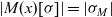 $|M(x)[\sigma]|=|\sigma_{M}|$
.
$|M(x)[\sigma]|=|\sigma_{M}|$
.
Corollary 59. Let t be a term in context
 $\boldsymbol{\Gamma};a$
with
$\boldsymbol{\Gamma};a$
with
 $(M:m)\in\boldsymbol{\Gamma}$
and
$(M:m)\in\boldsymbol{\Gamma}$
and
 $x\in\hom_{\mathcal{A}}(m,a)$
such that
$x\in\hom_{\mathcal{A}}(m,a)$
such that
 $\sigma:\boldsymbol{\Gamma}\rightarrow\boldsymbol{\Delta}$
unifies t and M(x). Then, either
$\sigma:\boldsymbol{\Gamma}\rightarrow\boldsymbol{\Delta}$
unifies t and M(x). Then, either
 $t=M(y)$
for some
$t=M(y)$
for some
 $y\in\hom_{\mathcal{A}}(m,a)$
, or
$y\in\hom_{\mathcal{A}}(m,a)$
, or
 $\boldsymbol{\Gamma};a\vdash t$
.
$\boldsymbol{\Gamma};a\vdash t$
.
Proof Since
 $t[\sigma]=M(x)[u]$
, we have
$t[\sigma]=M(x)[u]$
, we have
 $|t[\sigma]|=|M(x)[\sigma]|$
. Corollary 58 implies
$|t[\sigma]|=|M(x)[\sigma]|$
. Corollary 58 implies
 $|\sigma_{M}|\geq|t|+|\sigma_{M}|\times|t|_{M}$
. Therefore, either
$|\sigma_{M}|\geq|t|+|\sigma_{M}|\times|t|_{M}$
. Therefore, either
 $|t|_{M}=0$
and we conclude by Lemma 57, or
$|t|_{M}=0$
and we conclude by Lemma 57, or
 $|t|_{M}>0$
and
$|t|_{M}>0$
and
 $|t|=0$
, so that t is M(y) for some y.
$|t|=0$
, so that t is M(y) for some y.
6 Termination and completeness
6.1. Termination
In this section, we sketch an explicit argument to justify termination of our algorithm described in Figure 10. Note that the pruning and the unification phases are not mutually recursive: the latter depends on the former, but not conversely. Therefore, we can first show that the pruning phase terminates, and then that the unification does. Both phases involve three recursive calls (cf. the rules ![]() ,
, ![]() ,
, ![]() , and
, and ![]() ). In each phase, the second recursive call for splitting is not structurally recursive, making Agda unable to check termination. However, we can devise an adequate notion of input size so that for each recursive call, the inputs are strictly smaller than the inputs of the calling site. First, we define the size
). In each phase, the second recursive call for splitting is not structurally recursive, making Agda unable to check termination. However, we can devise an adequate notion of input size so that for each recursive call, the inputs are strictly smaller than the inputs of the calling site. First, we define the size
 $|\boldsymbol{\Gamma}|$
of a proper metacontext
$|\boldsymbol{\Gamma}|$
of a proper metacontext
 $\boldsymbol{\Gamma}$
as its length, while
$\boldsymbol{\Gamma}$
as its length, while
 $|\bot|=0$
by definition. We also recursively define the sizeFootnote
7
$|\bot|=0$
by definition. We also recursively define the sizeFootnote
7
 $||t||$
of a proper term t by
$||t||$
of a proper term t by
 $||M(x)||=1$
and
$||M(x)||=1$
and
 $||o(\vec{t})||=1+||\vec{t}||$
, with
$||o(\vec{t})||=1+||\vec{t}||$
, with
 $||\vec{t}||=\sum_{i}||t_{i}||$
. We also define the size of the error term
$||\vec{t}||=\sum_{i}||t_{i}||$
. We also define the size of the error term
 $||\mbox{!}||$
as 1. Note that no term is of size 0.
$||\mbox{!}||$
as 1. Note that no term is of size 0.
Definition 60. We say that a substitution
 $\sigma:\Gamma\rightarrow\Delta$
is monotone if
$\sigma:\Gamma\rightarrow\Delta$
is monotone if
 $||t[\sigma]||\leq||t||$
for any term well-formed in the metacontext
$||t[\sigma]||\leq||t||$
for any term well-formed in the metacontext
 $\Gamma$
.
$\Gamma$
.
Example 61. The error substitution
 $\mbox{!}$
is monotone since there is no term of size 0. A substitution
$\mbox{!}$
is monotone since there is no term of size 0. A substitution
 $\sigma:\boldsymbol{\Gamma}\rightarrow\boldsymbol{\Delta}$
such that
$\sigma:\boldsymbol{\Gamma}\rightarrow\boldsymbol{\Delta}$
such that
 $\sigma_{M}$
is a metavariable application for any
$\sigma_{M}$
is a metavariable application for any
 $(M:m)\in\boldsymbol{\Gamma}$
is monotone (as in the output of the rules
$(M:m)\in\boldsymbol{\Gamma}$
is monotone (as in the output of the rules ![]() and
and ![]() ).
).
Let us first quickly justify termination of the pruning phase.
Lemma 62. If there is a derivation tree of
 $\Gamma\vdash_{}\vec{t}\boldsymbol{:>}x\Rightarrow\vec{w};\sigma\dashv\Delta$
, then
$\Gamma\vdash_{}\vec{t}\boldsymbol{:>}x\Rightarrow\vec{w};\sigma\dashv\Delta$
, then
 $\sigma$
is monotone.
$\sigma$
is monotone.
Corollary 63. The pruning phase always terminates.
Proof Consider the above defined size of the input, which is a term t for ![]() , or a list of terms
, or a list of terms
 $\vec{t}$
for
$\vec{t}$
for ![]() . It is straightforward to check that the sizes of the inputs of recursive calls are strictly smaller thanks to the previous lemma. Let us detail the case of the rule
. It is straightforward to check that the sizes of the inputs of recursive calls are strictly smaller thanks to the previous lemma. Let us detail the case of the rule ![]() . We show that the input
. We show that the input
 $\delta[\sigma_{1}]$
of the second recursive call is smaller than the original input
$\delta[\sigma_{1}]$
of the second recursive call is smaller than the original input
 $t,\delta$
. Then,
$t,\delta$
. Then,

For termination of the main unification phase, we consider the size of the input to be the (lexicographic) pair
 $(|\Gamma|,||t||)$
for
$(|\Gamma|,||t||)$
for ![]() or
or
 $(|\Gamma|,||\vec{t}||)$
for
$(|\Gamma|,||\vec{t}||)$
for ![]() , given as input a pair of terms (t,t’) or lists of terms
, given as input a pair of terms (t,t’) or lists of terms
 $(\vec{t},\vec{t'})$
in the metacontext
$(\vec{t},\vec{t'})$
in the metacontext
 $\Gamma$
.
$\Gamma$
.
Lemma 64. If there is a derivation tree of
 $\Gamma\vdash_{}\vec{t}\boldsymbol{:>}x\Rightarrow\vec{w};\sigma\dashv\Delta$
or
$\Gamma\vdash_{}\vec{t}\boldsymbol{:>}x\Rightarrow\vec{w};\sigma\dashv\Delta$
or
 $\Gamma\vdash\vec{t}=\vec{u}\Rightarrow\sigma\dashv\Delta$
, then
$\Gamma\vdash\vec{t}=\vec{u}\Rightarrow\sigma\dashv\Delta$
, then
 $|\Gamma|\geq|\Delta|$
.
$|\Gamma|\geq|\Delta|$
.
Lemma 65. If there is a derivation tree of
 $\Gamma\vdash\vec{t}=\vec{u}\Rightarrow\sigma\dashv\Delta$
such that
$\Gamma\vdash\vec{t}=\vec{u}\Rightarrow\sigma\dashv\Delta$
such that
 $|\Gamma|=|\Delta|$
, then
$|\Gamma|=|\Delta|$
, then
 $\sigma$
is monotone.
$\sigma$
is monotone.
Corollary 66. The unification algorithm as defined in Figure 10 always terminates.
Proof It is straightforward to check that the sizes of the inputs of recursive calls are strictly smaller thanks to the previous lemmas. Let us detail the case of the rule ![]() . We show that the size
. We show that the size
 $(|\Delta|,||\delta_{1}[\sigma]||)$
of the second recursive call is strictly smaller than the size
$(|\Delta|,||\delta_{1}[\sigma]||)$
of the second recursive call is strictly smaller than the size
 $(|\Gamma|,||t_{1},\delta_{1}||)$
of the original input.
$(|\Gamma|,||t_{1},\delta_{1}||)$
of the original input.
If
 $|\Delta|<|\Gamma|$
, then we are done. Otherwise, by Lemma 64, we have
$|\Delta|<|\Gamma|$
, then we are done. Otherwise, by Lemma 64, we have
 $|\Delta|=|\Gamma|$
, and then,
$|\Delta|=|\Gamma|$
, and then,

6.2. Completeness
In this section, we explain why soundness (Sections 4 and 5) and termination (Section 6.1) entail completeness. Intuitively, one may worry that the algorithm fails in cases where it should not. In fact, we already checked in the previous sections that failure only occurs when there is no unifier, as expected. Indeed, failure is treated as a free “terminal” unifier, as explained in Section 3.1, by considering the category
 $\mathrm{MCon}(S)_{\bot}$
extending category
$\mathrm{MCon}(S)_{\bot}$
extending category
 $\mathrm{MCon}(S)$
with an error metacontext
$\mathrm{MCon}(S)$
with an error metacontext
 $\bot$
. Corollary 19 implies that since the algorithm terminates and computes the coequaliser in
$\bot$
. Corollary 19 implies that since the algorithm terminates and computes the coequaliser in
 $\mathrm{MCon}(S)_{\bot}$
, it always finds the most general unifier in
$\mathrm{MCon}(S)_{\bot}$
, it always finds the most general unifier in
 $\mathrm{MCon}(S)$
if it exists, and otherwise returns failure (i.e., the map to the terminal object
$\mathrm{MCon}(S)$
if it exists, and otherwise returns failure (i.e., the map to the terminal object
 $\bot$
).
$\bot$
).
7 Applications
In this section, we present various examples of pattern-friendly signatures.
We start in Section 7.1 with a variant of pure
 $\lambda$
-calculus where metavariable arguments are sets rather than lists. In Section 7.2, we present simply typed
$\lambda$
-calculus where metavariable arguments are sets rather than lists. In Section 7.2, we present simply typed
 $\lambda$
-calculus, as an example of syntax specified by a multi-sorted binding signature. We then explain in Section 7.3 how we can handle
$\lambda$
-calculus, as an example of syntax specified by a multi-sorted binding signature. We then explain in Section 7.3 how we can handle
 $\beta$
and
$\beta$
and
 $\eta$
equations by working on the normalised syntax. Next, we introduce an example of unification for ordered syntax in Section 7.4, and finally we present an example of polymorphic language such as System F, in Section 7.5.1.
$\eta$
equations by working on the normalised syntax. Next, we introduce an example of unification for ordered syntax in Section 7.4, and finally we present an example of polymorphic language such as System F, in Section 7.5.1.
7.1 Metavariable arguments as sets
If we think of the arguments of a metavariable as specifying the available variables in any order (as in Section 2.1), then it makes sense to assemble them in a set rather than in a list. This motivates considering the category
 $\mathcal{A}=\mathbb{I}$
whose objects are natural numbers and a morphism
$\mathcal{A}=\mathbb{I}$
whose objects are natural numbers and a morphism
 $n\rightarrow p$
is a subset of
$n\rightarrow p$
is a subset of
 $\{1,\dots,p\}$
of cardinality n. Equivalently,
$\{1,\dots,p\}$
of cardinality n. Equivalently,
 $\mathbb{I}$
can be taken as subcategory of
$\mathbb{I}$
can be taken as subcategory of
 $\mathbb{F}_{m}$
consisting of strictly increasing injections, or as the subcategory of the augmented simplex category consisting of injective functions. Then, a metavariable takes as argument a set of variables, rather than a list of distinct variables. In this approach, unifying two metavariables (see the rules
$\mathbb{F}_{m}$
consisting of strictly increasing injections, or as the subcategory of the augmented simplex category consisting of injective functions. Then, a metavariable takes as argument a set of variables, rather than a list of distinct variables. In this approach, unifying two metavariables (see the rules ![]() and
and ![]() ) amount to computing a set intersection.
) amount to computing a set intersection.
7.2 Simply typed
$\lambda$
-calculus

In this section, we present the example of simply typed
 $\lambda$
-calculus. Our treatment generalises to any multi-sorted binding signature (Fiore & Hur Reference Fiore and Hur2010).
$\lambda$
-calculus. Our treatment generalises to any multi-sorted binding signature (Fiore & Hur Reference Fiore and Hur2010).
Let T denote the set of simple types generated by a set of base types and a binary arrow type construction
 $-\Rightarrow-$
. Let us now describe the category
$-\Rightarrow-$
. Let us now describe the category
 $\mathcal{A}$
of arities, or scopes, and renamings between them. An arity
$\mathcal{A}$
of arities, or scopes, and renamings between them. An arity
 $\vec{\sigma}\rightarrow\tau$
consists of a list of input types
$\vec{\sigma}\rightarrow\tau$
consists of a list of input types
 $\vec{\sigma}$
and an output type
$\vec{\sigma}$
and an output type
 $\tau$
. A term t in
$\tau$
. A term t in
 $\vec{\sigma}\rightarrow\tau$
considered as a scope is intuitively a well-typed term t of type
$\vec{\sigma}\rightarrow\tau$
considered as a scope is intuitively a well-typed term t of type
 $\tau$
potentially using variables whose types are specified by
$\tau$
potentially using variables whose types are specified by
 $\vec{\sigma}$
. A valid choice of arguments for a metavariable
$\vec{\sigma}$
. A valid choice of arguments for a metavariable
 $M:(\vec{\sigma}\rightarrow\tau)$
in scope
$M:(\vec{\sigma}\rightarrow\tau)$
in scope
 $\vec{\sigma}'\rightarrow\tau'$
first requires
$\vec{\sigma}'\rightarrow\tau'$
first requires
 $\tau=\tau'$
and consists of an injective renaming
$\tau=\tau'$
and consists of an injective renaming
 $\vec{r}$
between
$\vec{r}$
between
 $\vec{\sigma}=(\sigma_{1},\dots,\sigma_{m})$
and
$\vec{\sigma}=(\sigma_{1},\dots,\sigma_{m})$
and
 $\vec{\sigma}'=(\sigma'_{1},\dots,\sigma'_{n})$
, that is, a choice of distinct positions
$\vec{\sigma}'=(\sigma'_{1},\dots,\sigma'_{n})$
, that is, a choice of distinct positions
 $(r_{1},\dots,r_{m})$
in
$(r_{1},\dots,r_{m})$
in
 $\{1,\dots,n\}$
such that
$\{1,\dots,n\}$
such that
 $\vec{\sigma}=\sigma'_{\vec{r}}$
.
$\vec{\sigma}=\sigma'_{\vec{r}}$
.
This discussion determines the category of arities as
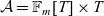 $\mathcal{A}=\mathbb{F}_{m}[T]\times T$
, where
$\mathcal{A}=\mathbb{F}_{m}[T]\times T$
, where
 $\mathbb{F}_{m}[T]$
is the category of finite lists of elements of T and injective renamings between them. Table 1 summarises the GB-signature specifying the syntax, where
$\mathbb{F}_{m}[T]$
is the category of finite lists of elements of T and injective renamings between them. Table 1 summarises the GB-signature specifying the syntax, where
 $|\vec{\sigma}|_{\tau}$
denotes the number (as a cardinal set) of occurrences of
$|\vec{\sigma}|_{\tau}$
denotes the number (as a cardinal set) of occurrences of
 $\tau$
in
$\tau$
in
 $\vec{\sigma}$
. The middle column associates a subset of the operation symbols to each typing rule: the total set of operation symbols is recovered by computing the (disjoint) union of them. The last column gives the list
$\vec{\sigma}$
. The middle column associates a subset of the operation symbols to each typing rule: the total set of operation symbols is recovered by computing the (disjoint) union of them. The last column gives the list
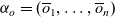 $\alpha_{o}=(\overline{o}_{1},\dots,\overline{o}_{n})$
for each operation symbol o.
$\alpha_{o}=(\overline{o}_{1},\dots,\overline{o}_{n})$
for each operation symbol o.
Simply typed
 $\lambda$
-calculus (Section 7.2)
$\lambda$
-calculus (Section 7.2)

Proposition 67. The induced signature is pattern-friendly.
Proof Because we consider injective renamings, it is easy to check that every morphism in
 $\mathcal{A}$
is monomorphic. Moreover, the projection functor
$\mathcal{A}$
is monomorphic. Moreover, the projection functor
 $\mathcal{A}\rightarrow\mathbb{F}_{m}[T]$
creates finite connected limits. For instance, consider an equaliser diagram in
$\mathcal{A}\rightarrow\mathbb{F}_{m}[T]$
creates finite connected limits. For instance, consider an equaliser diagram in
 $\mathcal{A}$
, that is, two parallel morphisms
$\mathcal{A}$
, that is, two parallel morphisms
 $\vec{x},\vec{y}$
between
$\vec{x},\vec{y}$
between
 $\vec{\sigma}\rightarrow\tau$
and
$\vec{\sigma}\rightarrow\tau$
and
 $\vec{\sigma}'\rightarrow\tau'$
. First,
$\vec{\sigma}'\rightarrow\tau'$
. First,
 $\tau=\tau'$
, and then we compute the equaliser of
$\tau=\tau'$
, and then we compute the equaliser of
 $\vec{\sigma}$
and
$\vec{\sigma}$
and
 $\vec{\sigma}'$
in
$\vec{\sigma}'$
in
 $\mathbb{F}_{m}[T]$
following the same process as in pure
$\mathbb{F}_{m}[T]$
following the same process as in pure
 $\lambda$
-calculus: we construct the vector
$\lambda$
-calculus: we construct the vector
 $\vec{z}$
of common positions between
$\vec{z}$
of common positions between
 $\vec{x}$
and
$\vec{x}$
and
 $\vec{y}$
, thus satisfying
$\vec{y}$
, thus satisfying
 $x_{\vec{z}}=y_{\vec{z}}$
. Then,
$x_{\vec{z}}=y_{\vec{z}}$
. Then,
 $\vec{z}$
defines a morphism from
$\vec{z}$
defines a morphism from
 $\sigma_{\vec{z}}$
to
$\sigma_{\vec{z}}$
to
 $\vec{\sigma}$
, which is the equaliser of
$\vec{\sigma}$
, which is the equaliser of
 $\vec{x}$
and
$\vec{x}$
and
 $\vec{y}$
in
$\vec{y}$
in
 $\mathbb{F}_{m}[T]$
. It is straightforward to check that it is also the equaliser in
$\mathbb{F}_{m}[T]$
. It is straightforward to check that it is also the equaliser in
 $\mathcal{A}=\mathbb{F}_{m}[T]\times T$
.
$\mathcal{A}=\mathbb{F}_{m}[T]\times T$
.
Next, every
 $\mathcal{O}_{n}$
preserve finite connected limits by Lemma 47 because they are all coproduct of representable functors (as shown below), which preserve limits by Mac Lane (Reference Mac Lane1998, Theorem V.4.1):
$\mathcal{O}_{n}$
preserve finite connected limits by Lemma 47 because they are all coproduct of representable functors (as shown below), which preserve limits by Mac Lane (Reference Mac Lane1998, Theorem V.4.1):
 \begin{align*}\mathcal{O}_{0}(-) & \cong\coprod_{\tau\in T}\hom_{\mathcal{A}}(\tau\rightarrow\tau,-)\\\mathcal{O}_{1}(-) & \cong\coprod_{\tau_{1},\tau_{2}\in T}\hom_{\mathcal{A}}(\cdot\rightarrow\tau_{1}\Rightarrow\tau_{2},-)\\\mathcal{O}_{2}(-) & \cong\coprod_{\tau,\tau'\in T}\hom_{\mathcal{A}}(\cdot\rightarrow\tau,-)\\\mathcal{O}_{3+n}(-) & \cong\emptyset\end{align*}
Note that
 $\alpha_{3+n,i}:\emptyset\rightarrow\mathcal{A}$
vacuously preserves finite connected limits. It remains to show that
$\alpha_{3+n,i}:\emptyset\rightarrow\mathcal{A}$
vacuously preserves finite connected limits. It remains to show that
 $\alpha_{1,1}$
,
$\alpha_{1,1}$
,
 $\alpha_{2,1}$
, and
$\alpha_{2,1}$
, and
 $\alpha_{2,2}$
also preserve them. First, we observe that the domains of those functors are isomorphic to
$\alpha_{2,2}$
also preserve them. First, we observe that the domains of those functors are isomorphic to
 $\mathbb{F}_{m}[T]\times T^{2}$
. More specifically,
$\mathbb{F}_{m}[T]\times T^{2}$
. More specifically,
 \begin{align*}\int\mathcal{O}_{i} & \cong\mathbb{F}_{m}[T]\times T^{2} & i\in\{1,2\}\\(\vec{\sigma}\rightarrow\tau_{1}\Rightarrow\tau_{2},l_{\tau_{1},\tau_{2}}) & \mapsto(\vec{\sigma},\tau_{1},\tau_{2}) & i=1\\(\vec{\sigma}\rightarrow\tau,a_{\tau'}) & \mapsto(\vec{\sigma},\tau,\tau') & i=2\end{align*}
Precomposed with the reverse isomorphisms, the functors
 $\alpha_{1,1},\alpha_{2,1},\alpha_{2,2}:\int\mathcal{O}_{n}\rightarrow\mathcal{A}$
induce the three below left functors
$\alpha_{1,1},\alpha_{2,1},\alpha_{2,2}:\int\mathcal{O}_{n}\rightarrow\mathcal{A}$
induce the three below left functors
 $\beta_{1,1}$
,
$\beta_{1,1}$
,
 $\beta_{2,1}$
, and
$\beta_{2,1}$
, and
 $\beta_{2,2}$
.
$\beta_{2,2}$
.

Now, finite connected limits in
 $\mathbb{F}_{m}[T]\times T^{n}$
are computed in
$\mathbb{F}_{m}[T]\times T^{n}$
are computed in
 $\mathbb{F}_{m}[T]$
. Therefore, to conclude that the functors
$\mathbb{F}_{m}[T]$
. Therefore, to conclude that the functors
 $\beta_{n,i}$
listed above left preserve those limits, it is enough to show that given
$\beta_{n,i}$
listed above left preserve those limits, it is enough to show that given
 $\tau_{1},\tau_{2}\in T$
, the compositions
$\tau_{1},\tau_{2}\in T$
, the compositions
 $\mathbb{F}_{m}[T]\xrightarrow{(-,\tau_{1},\tau_{2})}\mathbb{F}_{m}[T]\times T^{2}\xrightarrow{\beta_{n,i}}\mathbb{F}_{m}[T]\times T\rightarrow\mathbb{F}_{m}[T]$
listed above right do so. It is obvious for the last two functors, and it is straightforward to check for the first functor, by investigating the constructions of equalisers and pullbacks.
$\mathbb{F}_{m}[T]\xrightarrow{(-,\tau_{1},\tau_{2})}\mathbb{F}_{m}[T]\times T^{2}\xrightarrow{\beta_{n,i}}\mathbb{F}_{m}[T]\times T\rightarrow\mathbb{F}_{m}[T]$
listed above right do so. It is obvious for the last two functors, and it is straightforward to check for the first functor, by investigating the constructions of equalisers and pullbacks.
It follows that the generic pattern unification algorithm applies. Equalisers and pullbacks are computed following the same pattern as in pure
 $\lambda$
-calculus. For example, to unify
$\lambda$
-calculus. For example, to unify
 $M(\vec{x})$
and
$M(\vec{x})$
and
 $M(\vec{y})$
, we first compute the vector
$M(\vec{y})$
, we first compute the vector
 $\vec{z}$
of common positions between
$\vec{z}$
of common positions between
 $\vec{x}$
and
$\vec{x}$
and
 $\vec{y}$
, thus satisfying
$\vec{y}$
, thus satisfying
 $x_{\vec{z}}=y_{\vec{z}}$
. Then, the most general unifier maps
$x_{\vec{z}}=y_{\vec{z}}$
. Then, the most general unifier maps
 $M:(\vec{\sigma}\rightarrow\tau)$
to the term
$M:(\vec{\sigma}\rightarrow\tau)$
to the term
 $P(\vec{z})$
, where the arity
$P(\vec{z})$
, where the arity
 $\vec{\sigma}'\rightarrow\tau'$
of the fresh metavariable P is the only possible choice such that
$\vec{\sigma}'\rightarrow\tau'$
of the fresh metavariable P is the only possible choice such that
 $P(\vec{z})$
is a valid term in the scope
$P(\vec{z})$
is a valid term in the scope
 $\vec{\sigma}\rightarrow\tau$
, that is,
$\vec{\sigma}\rightarrow\tau$
, that is,
 $\tau'=\tau$
and
$\tau'=\tau$
and
 $\vec{\sigma}'=\sigma_{\vec{z}}$
.
$\vec{\sigma}'=\sigma_{\vec{z}}$
.
7.3 Simply typed
$\lambda$
-calculus modulo
$\beta$
$\eta$


In this section, we explain how we account for Miller’s original setting: simply typed
 $\lambda$
-calculus modulo
$\lambda$
-calculus modulo
 $\beta$
and
$\beta$
and
 $\eta$
-equations. We follow Cheney’s presentation of the equation-free syntax of
$\eta$
-equations. We follow Cheney’s presentation of the equation-free syntax of
 $\beta$
-short
$\beta$
-short
 $\eta$
-long normal forms with metavariables (Cheney, Reference Cheney2005, Section 2.1). The normals forms have the following shape, where z denotes a variable,
$\eta$
-long normal forms with metavariables (Cheney, Reference Cheney2005, Section 2.1). The normals forms have the following shape, where z denotes a variable,
 $\vec{x}$
denotes a vector of distinct variables and M denotes a metavariable:
$\vec{x}$
denotes a vector of distinct variables and M denotes a metavariable:
 \[t::=\lambda\vec{y}.z\vec{t}|\lambda\vec{y}.M\vec{x}\]
This syntax is closed under substitution of metavariables, modulo
 $\beta$
-normalisation. For example, replacing M by
$\beta$
-normalisation. For example, replacing M by
 $\lambda ww'.z\vec{t}$
in
$\lambda ww'.z\vec{t}$
in
 $\lambda\vec{y}.Mxx'$
yields a
$\lambda\vec{y}.Mxx'$
yields a
 $\beta$
-reducible term
$\beta$
-reducible term
 $\lambda\vec{y}.(\lambda ww'.z\vec{t})xx'$
which yields a normal form after two
$\lambda\vec{y}.(\lambda ww'.z\vec{t})xx'$
which yields a normal form after two
 $\beta$
-reductions.
$\beta$
-reductions.
Remark 68. Hereditary substitutions (Watkins et al., 2003; Abel & Pientka, 2011) is a refined implementation of substitution of normal forms that perform
 $\beta$
-normalisation on the fly so that the output is a normal form. It works for second-order metavariables, where arguments of metavariables are arbitrary terms. The pattern fragment is a simple case: the only
$\beta$
-normalisation on the fly so that the output is a normal form. It works for second-order metavariables, where arguments of metavariables are arbitrary terms. The pattern fragment is a simple case: the only
 $\beta$
-redices introduced by substituting a metavariable are the application of a
$\beta$
-redices introduced by substituting a metavariable are the application of a
 $\lambda$
-abstraction to variables.
$\lambda$
-abstraction to variables.
We now explain how this syntax of normal forms can be specified by a GB-signature. The associated metavariable substitution is then hereditary in the sense of Remark 68, since the syntax generated by any GB-signature is always stable under metavariable substitution.
Notation 69. We denote a type
 $\sigma_{1}\Rightarrow\dots\Rightarrow\sigma_{n}\Rightarrow\iota$
by
$\sigma_{1}\Rightarrow\dots\Rightarrow\sigma_{n}\Rightarrow\iota$
by
 $\vec{\sigma}\Rightarrow\iota$
, where
$\vec{\sigma}\Rightarrow\iota$
, where
 $\iota$
is a base type. Note that any type can be written in this way, uniquely.
$\iota$
is a base type. Note that any type can be written in this way, uniquely.
We take the same notion of scope as in the previous section: a term well-formed in scope
 $\vec{\sigma}\rightarrow\tau$
will correspond to a normal form of type
$\vec{\sigma}\rightarrow\tau$
will correspond to a normal form of type
 $\tau$
with free variables of types
$\tau$
with free variables of types
 $\vec{\sigma}$
.
$\vec{\sigma}$
.
Definition 70. We say that a metavariable of arity
 $\vec{\sigma}\rightarrow(\vec{\tau}\Rightarrow\iota)$
has type
$\vec{\sigma}\rightarrow(\vec{\tau}\Rightarrow\iota)$
has type
 $\tau'$
when
$\tau'$
when
 $\tau'$
is
$\tau'$
is
 $\vec{\sigma},\vec{\tau}\Rightarrow\iota$
.
$\vec{\sigma},\vec{\tau}\Rightarrow\iota$
.
We choose a notion of scope morphism different from that of the previous section, so that the introduction rule of metavariables matches the below typing rule for a metavariable term
 $\lambda\vec{y}.M\vec{x}$
, given a metavariable M of type
$\lambda\vec{y}.M\vec{x}$
, given a metavariable M of type
 $\vec{\tau}\Rightarrow\iota$
.
$\vec{\tau}\Rightarrow\iota$
.

Assuming that the arity of M is
 $\vec{\tau}_{1}\rightarrow\vec{\tau_{2}}\Rightarrow\iota$
with
$\vec{\tau}_{1}\rightarrow\vec{\tau_{2}}\Rightarrow\iota$
with
 $\vec{\tau}=\vec{\tau}_{1},\vec{\tau}_{2}$
, this means that a scope morphism from
$\vec{\tau}=\vec{\tau}_{1},\vec{\tau}_{2}$
, this means that a scope morphism from
 $\vec{\tau}_{1}\rightarrow(\vec{\tau_{2}}\Rightarrow\iota)$
to
$\vec{\tau}_{1}\rightarrow(\vec{\tau_{2}}\Rightarrow\iota)$
to
 $\vec{\sigma}\rightarrow(\vec{\sigma'}\Rightarrow\iota')$
should be empty unless
$\vec{\sigma}\rightarrow(\vec{\sigma'}\Rightarrow\iota')$
should be empty unless
 $\iota=\iota'$
. In that case, a morphism is given by a choice of distinct variables of types
$\iota=\iota'$
. In that case, a morphism is given by a choice of distinct variables of types
 $\vec{\tau}=\vec{\tau_{1}},\vec{\tau}_{2}$
in
$\vec{\tau}=\vec{\tau_{1}},\vec{\tau}_{2}$
in
 $\vec{\sigma},\vec{\sigma}'$
, that is, a morphism in
$\vec{\sigma},\vec{\sigma}'$
, that is, a morphism in
 $\mathbb{F}_{m}[T]$
between those two lists of types. We therefore arrive to the following definition.
$\mathbb{F}_{m}[T]$
between those two lists of types. We therefore arrive to the following definition.
Definition 71. The category of scopes
 $\mathcal{A}$
has pairs consisting of an object
$\mathcal{A}$
has pairs consisting of an object
 $\vec{\sigma}$
of
$\vec{\sigma}$
of
 $\mathbb{F}_{m}[T]$
and an element
$\mathbb{F}_{m}[T]$
and an element
 $\tau$
of T as objects. We denote such a pair by
$\tau$
of T as objects. We denote such a pair by
 $\vec{\sigma}\rightarrow\tau$
. A morphism between
$\vec{\sigma}\rightarrow\tau$
. A morphism between
 $\vec{\sigma}\rightarrow(\vec{\tau}\Rightarrow\iota)$
and
$\vec{\sigma}\rightarrow(\vec{\tau}\Rightarrow\iota)$
and
 $\vec{\sigma}'\rightarrow(\vec{\tau}'\Rightarrow\iota')$
is a morphism between
$\vec{\sigma}'\rightarrow(\vec{\tau}'\Rightarrow\iota')$
is a morphism between
 $\vec{\sigma},\vec{\tau}\rightarrow\iota$
and
$\vec{\sigma},\vec{\tau}\rightarrow\iota$
and
 $\vec{\sigma}',\vec{\tau}'\rightarrow\iota'$
in
$\vec{\sigma}',\vec{\tau}'\rightarrow\iota'$
in
 $\mathbb{F}_{m}[T]\times B$
. Composition and identities are defined as in
$\mathbb{F}_{m}[T]\times B$
. Composition and identities are defined as in
 $\mathbb{F}_{m}[T]\times B$
.
$\mathbb{F}_{m}[T]\times B$
.
This definition readily entails that
 $\mathcal{A}$
is equivalent to
$\mathcal{A}$
is equivalent to
 $\mathbb{F}_{m}[T]\times B$
.
$\mathbb{F}_{m}[T]\times B$
.
We have specified the category of scopes so that we get a suitable introduction rule for metavariables. It remains to provide a GB-signature on top of
 $\mathcal{A}$
that accounts for the construction
$\mathcal{A}$
that accounts for the construction
 $\lambda\vec{y}.x\vec{t}$
, with the corresponding below typing rule:
$\lambda\vec{y}.x\vec{t}$
, with the corresponding below typing rule:
 \[\dfrac{x:(\vec{\tau}\Rightarrow\iota)\in(\vec{z}:\vec{\sigma},\vec{y}:\vec{\sigma'})\qquad\vec{z}:\vec{\sigma},\vec{y}:\vec{\sigma'}\vdash\vec{t}:\vec{\tau}}{\vec{z}:\vec{\sigma}\vdash\lambda\vec{y}.x\vec{t}:\vec{\sigma'}\Rightarrow\iota}\]
The following components induce a GB-signature that generates the same base syntax:
 \begin{align*}O(\vec{\sigma}\rightarrow\tau) & =\{l_{x,\tau_{1},\dots,\tau_{n},\vec{\sigma'},\iota}|\tau=(\vec{\sigma'}\Rightarrow\iota),x\in|\vec{\sigma},\vec{\sigma'}|_{\vec{\tau}\Rightarrow\iota}\}\\\alpha_{l_{x,\tau_{1},\dots,\tau_{n},\vec{\sigma'},\iota}} & =\left(\begin{array}{c}\vec{\sigma},\vec{\sigma'}\rightarrow\tau_{1}\\\dots\\\vec{\sigma},\vec{\sigma'}\rightarrow\tau_{n}\end{array}\right)\end{align*}
7.4 Ordered
$\lambda$
-calculus

Our setting handles linear ordered
 $\lambda$
-calculus, consisting of
$\lambda$
-calculus, consisting of
 $\lambda$
-terms using all the variables in context. In this context, a metavariable M of arity
$\lambda$
-terms using all the variables in context. In this context, a metavariable M of arity
 $m\in\mathbb{N}$
can only be used in the scope m, and there is no freedom in choosing the arguments of a metavariable application, since all the variables must be used, in order. Thus, there is no need to even mention those arguments in the syntax. It is thus not surprising that ordered
$m\in\mathbb{N}$
can only be used in the scope m, and there is no freedom in choosing the arguments of a metavariable application, since all the variables must be used, in order. Thus, there is no need to even mention those arguments in the syntax. It is thus not surprising that ordered
 $\lambda$
-calculus is already handled by first-order unification, where metavariables do not take any argument, by considering ordered
$\lambda$
-calculus is already handled by first-order unification, where metavariables do not take any argument, by considering ordered
 $\lambda$
-calculus as a multi-sorted Lawvere theory where the sorts are the scopes, and the syntax is generated by operations
$\lambda$
-calculus as a multi-sorted Lawvere theory where the sorts are the scopes, and the syntax is generated by operations
 $L_{n}\times L_{m}\rightarrow L_{n+m}$
and abstractions
$L_{n}\times L_{m}\rightarrow L_{n+m}$
and abstractions
 $L_{n+1}\rightarrow L_{n}$
.
$L_{n+1}\rightarrow L_{n}$
.
Our generalisation can handle calculi combining ordered and unrestricted variables, such as the calculus underlying ordered linear logic described in Polakow and Pfenning (Reference Polakow and Pfenning2000). In this section, we detail this specific example. Note that this does not fit into Schack–Nielsen and Schürman’s pattern unification algorithm (Schack-Nielsen &Schürmann, Reference Schack-Nielsen and Schürmann2010) for linear types where exchange is allowed (the order of their variables does not matter).
The set T of types is generated by a set of atomic types and two binary arrow type constructions
 $\Rightarrow$
and
$\Rightarrow$
and
 $\twoheadrightarrow$
. The syntax extends pure
$\twoheadrightarrow$
. The syntax extends pure
 $\lambda$
-calculus with a distinct application
$\lambda$
-calculus with a distinct application
 $t^{>}\ u$
and abstraction
$t^{>}\ u$
and abstraction
 $\lambda^{>}u$
. Variables contexts are of the shape
$\lambda^{>}u$
. Variables contexts are of the shape
 $\vec{\sigma}|\vec{\omega}\rightarrow\tau$
, where
$\vec{\sigma}|\vec{\omega}\rightarrow\tau$
, where
 $\vec{\sigma}$
,
$\vec{\sigma}$
,
 $\vec{\omega}$
, and
$\vec{\omega}$
, and
 $\tau$
are taken in T. The idea is that a term in such a context has type
$\tau$
are taken in T. The idea is that a term in such a context has type
 $\tau$
and must use all the variables of
$\tau$
and must use all the variables of
 $\vec{\omega}$
in order but is free to use any of the variables in
$\vec{\omega}$
in order but is free to use any of the variables in
 $\vec{\sigma}$
. Assuming a metavariable M of arity
$\vec{\sigma}$
. Assuming a metavariable M of arity
 $\vec{\sigma}|\vec{\omega}\rightarrow\tau$
, the above discussion about ordered
$\vec{\sigma}|\vec{\omega}\rightarrow\tau$
, the above discussion about ordered
 $\lambda$
-calculus justifies that there is no need to specify the arguments for
$\lambda$
-calculus justifies that there is no need to specify the arguments for
 $\vec{\omega}$
when applying M. Thus, a metavariable application
$\vec{\omega}$
when applying M. Thus, a metavariable application
 $M(\vec{x})$
in the scope
$M(\vec{x})$
in the scope
 $\vec{\sigma}'|\vec{\omega}'\rightarrow\tau'$
is well-formed if
$\vec{\sigma}'|\vec{\omega}'\rightarrow\tau'$
is well-formed if
 $\tau=\tau'$
and
$\tau=\tau'$
and
 $\vec{x}$
is an injective renaming from
$\vec{x}$
is an injective renaming from
 $\vec{\sigma}$
to
$\vec{\sigma}$
to
 $\vec{\sigma}'$
. Therefore, we take
$\vec{\sigma}'$
. Therefore, we take
 $\mathcal{A}=\mathbb{F}_{m}[T]\times T^{*}\times T$
for the category of arities, where
$\mathcal{A}=\mathbb{F}_{m}[T]\times T^{*}\times T$
for the category of arities, where
 $\mathbb{F}_{m}[T]$
accounts for the unrestricted variables, while
$\mathbb{F}_{m}[T]$
accounts for the unrestricted variables, while
 $T^{*}$
accounts for the linear ones: it denotes the discrete category whose objects are lists of elements of T. The remaining components of the GB-signature are specified in Table 2, following the same convention as in Table 1. We alternate typing rules for the unrestricted and the ordered fragments (variables, application, abstraction).
$T^{*}$
accounts for the linear ones: it denotes the discrete category whose objects are lists of elements of T. The remaining components of the GB-signature are specified in Table 2, following the same convention as in Table 1. We alternate typing rules for the unrestricted and the ordered fragments (variables, application, abstraction).
Ordered
 $\lambda$
-calculus (Section 7.4)
$\lambda$
-calculus (Section 7.4)

Pullbacks and equalisers are computed essentially as in Section 7.2. For example, the most general unifier of
 $M(\vec{x})$
and
$M(\vec{x})$
and
 $M(\vec{y})$
maps M to
$M(\vec{y})$
maps M to
 $P(\vec{z})$
where
$P(\vec{z})$
where
 $\vec{z}$
is the vector of common positions of
$\vec{z}$
is the vector of common positions of
 $\vec{x}$
and
$\vec{x}$
and
 $\vec{y}$
, and P is a fresh metavariable of arity
$\vec{y}$
, and P is a fresh metavariable of arity
 $\sigma_{\vec{z}}|\vec{\omega}\rightarrow\tau$
.
$\sigma_{\vec{z}}|\vec{\omega}\rightarrow\tau$
.
7.5 Intrinsic polymorphic syntax
7.5.1 Syntactic System F
We present intrinsic System F, in the spirit of Hamana (Reference Hamana2011). The Agda implementation of the pattern-friendly GB-signature can be found in the Supplementary Material.
The syntax of types in type scope n is inductively generated as follows, following the de Bruijn level convention:
 \[\dfrac{1\leq i\leq n}{n\vdash i}\qquad\dfrac{n\vdash t\quad n\vdash u}{n\vdash t\Rightarrow u}\qquad\dfrac{n+1\vdash t}{n\vdash\forall t}\]
Let
 $S:\mathbb{F}_{m}\rightarrow\mathrm{Set}$
be the functor mapping n to the set
$S:\mathbb{F}_{m}\rightarrow\mathrm{Set}$
be the functor mapping n to the set
 $S_{n}$
of types for system F taking free type variables in
$S_{n}$
of types for system F taking free type variables in
 $\{1,\dots,n\}$
. In other words,
$\{1,\dots,n\}$
. In other words,
 $S_{n}=\{\tau|n\vdash\tau\}$
. Intuitively, a metavariable arity
$S_{n}=\{\tau|n\vdash\tau\}$
. Intuitively, a metavariable arity
 $n|\vec{\sigma}\rightarrow\tau$
specifies the number n of free type variables, the list of input types
$n|\vec{\sigma}\rightarrow\tau$
specifies the number n of free type variables, the list of input types
 $\vec{\sigma}$
, and the output type
$\vec{\sigma}$
, and the output type
 $\tau$
, all living in
$\tau$
, all living in
 $S_{n}$
. This provides the underlying set of objects of the category
$S_{n}$
. This provides the underlying set of objects of the category
 $\mathcal{A}$
of arities. A term t in
$\mathcal{A}$
of arities. A term t in
 $n|\vec{\sigma}\rightarrow\tau$
considered as a scope is intuitively a well-typed term of type
$n|\vec{\sigma}\rightarrow\tau$
considered as a scope is intuitively a well-typed term of type
 $\tau$
potentially involving ground variables of type
$\tau$
potentially involving ground variables of type
 $\vec{\sigma}$
and type variables in
$\vec{\sigma}$
and type variables in
 $\{1,\dots,n\}$
.
$\{1,\dots,n\}$
.
A metavariable
 $M:(n|\sigma_{1},\dots,\sigma_{p}\rightarrow\tau)$
in the scope
$M:(n|\sigma_{1},\dots,\sigma_{p}\rightarrow\tau)$
in the scope
 $n'|\vec{\sigma}'\rightarrow\tau'$
must be supplied with a choice
$n'|\vec{\sigma}'\rightarrow\tau'$
must be supplied with a choice
 $(\eta_{1},\dots,\eta_{n})$
of n distinct type variables among the set
$(\eta_{1},\dots,\eta_{n})$
of n distinct type variables among the set
 $\{1,\dots n'\}$
such that
$\{1,\dots n'\}$
such that
 $\tau[\vec{\eta}]=\tau'$
, as well as an injective renaming
$\tau[\vec{\eta}]=\tau'$
, as well as an injective renaming
 $\vec{\sigma}[\vec{\eta}]\rightarrow\vec{\sigma}'$
, that is, a list of distinct positions
$\vec{\sigma}[\vec{\eta}]\rightarrow\vec{\sigma}'$
, that is, a list of distinct positions
 $r_{1},\dots,r_{p}$
such that
$r_{1},\dots,r_{p}$
such that
 $\vec{\sigma}[\vec{\eta}]=\sigma'_{\vec{r}}$
.
$\vec{\sigma}[\vec{\eta}]=\sigma'_{\vec{r}}$
.
This defines the data for a morphism in
 $\mathcal{A}$
between
$\mathcal{A}$
between
 $(n|\vec{\sigma}\rightarrow\tau)$
and
$(n|\vec{\sigma}\rightarrow\tau)$
and
 $(n'|\vec{\sigma}'\rightarrow\tau')$
. The intrinsic syntax of system F can then be specified as in Table 3, following the same convention as in Table 1. The induced GB-signature is pattern-friendly. For example, morphisms in
$(n'|\vec{\sigma}'\rightarrow\tau')$
. The intrinsic syntax of system F can then be specified as in Table 3, following the same convention as in Table 1. The induced GB-signature is pattern-friendly. For example, morphisms in
 $\mathcal{A}$
are easily seen to be monomorphic; we detail in Section 7.5.3 the proof that
$\mathcal{A}$
are easily seen to be monomorphic; we detail in Section 7.5.3 the proof that
 $\mathcal{A}$
has finite connected limits.
$\mathcal{A}$
has finite connected limits.
The (pattern-friendly) GB-signature of (syntactic) System F (Section 7.5.1)

Pullbacks and equalisers in
 $\mathcal{A}$
are essentially computed as in Section 7.2, by computing the vector of common (value) positions. For example, given a metavariable M of arity
$\mathcal{A}$
are essentially computed as in Section 7.2, by computing the vector of common (value) positions. For example, given a metavariable M of arity
 $m|\vec{\sigma}\rightarrow\tau$
, to unify
$m|\vec{\sigma}\rightarrow\tau$
, to unify
 $M(\vec{w}|\vec{x})$
with
$M(\vec{w}|\vec{x})$
with
 $M(\vec{y}|\vec{z})$
, we compute the vector of common positions
$M(\vec{y}|\vec{z})$
, we compute the vector of common positions
 $\vec{p}$
between
$\vec{p}$
between
 $\vec{w}$
and
$\vec{w}$
and
 $\vec{y}$
, and the vector of common positions
$\vec{y}$
, and the vector of common positions
 $\vec{q}$
between
$\vec{q}$
between
 $\vec{x}$
and
$\vec{x}$
and
 $\vec{z}$
. Then, the most general unifier maps M to the term
$\vec{z}$
. Then, the most general unifier maps M to the term
 $P(\vec{p}|\vec{q})$
, where P is a fresh metavariable. Its arity
$P(\vec{p}|\vec{q})$
, where P is a fresh metavariable. Its arity
 $m'|\vec{\sigma}'\rightarrow\tau'$
is the only possible one for
$m'|\vec{\sigma}'\rightarrow\tau'$
is the only possible one for
 $P(\vec{p}|\vec{q})$
to be well-formed in the scope
$P(\vec{p}|\vec{q})$
to be well-formed in the scope
 $m|\vec{\sigma}\rightarrow\tau$
, that is, m’ is the size of
$m|\vec{\sigma}\rightarrow\tau$
, that is, m’ is the size of
 $\vec{p}$
, while
$\vec{p}$
, while
 $\tau'=\tau[p_{i}\mapsto i]$
and
$\tau'=\tau[p_{i}\mapsto i]$
and ![]() .
.
7.5.2 System F modulo
$\beta\eta$

In this section, we sketch how we can handle System F modulo
 $\beta\eta$
in the spirit of Section 7.3, by devising a signature for normal forms. To make the syntax more legible, we depart from the previous presentation and instead consider System F as a pure type system. We also ignore the de Bruijn encoding. A scope is now of the shape
$\beta\eta$
in the spirit of Section 7.3, by devising a signature for normal forms. To make the syntax more legible, we depart from the previous presentation and instead consider System F as a pure type system. We also ignore the de Bruijn encoding. A scope is now of the shape
 $\vec{y}:\vec{u}\rightarrow\tau$
, where
$\vec{y}:\vec{u}\rightarrow\tau$
, where
-
•
$\vec{y}:\vec{u}$
is a list of variable declarations
$y_{1}:u_{1},\dots,y_{n}:u_{n}$
where
$u_{i}$
is either
$*$
, meaning that
$y_{i}$
is a type variable, or a type which is well-formed in context involving all the type variables occuring before
$y_{i}$
in the scope; -
• •
$\tau$
is a type well-formed in
$\vec{y}:\vec{u}$
.


We use the notation
 $\prod(\alpha:u).\tau$
, where
$\prod(\alpha:u).\tau$
, where
 $\tau$
may depend on
$\tau$
may depend on
 $\alpha$
, to mean either
$\alpha$
, to mean either
 $\forall\alpha.\tau_{2}$
in case
$\forall\alpha.\tau_{2}$
in case
 $u=*$
, or
$u=*$
, or
 $u\Rightarrow\tau$
otherwise (in the latter case,
$u\Rightarrow\tau$
otherwise (in the latter case,
 $\tau$
does not depend on
$\tau$
does not depend on
 $\alpha$
).
$\alpha$
).
Note that any type can be written as
 $\prod(y_{1}:u_{1})\prod\dots\prod(y_{n}:u_{n}).\iota$
, abbreviated as
$\prod(y_{1}:u_{1})\prod\dots\prod(y_{n}:u_{n}).\iota$
, abbreviated as
 $\prod(\vec{y}:\vec{u}).\iota$
, where
$\prod(\vec{y}:\vec{u}).\iota$
, where
 $\iota$
is a type variable. Any scope
$\iota$
is a type variable. Any scope
 $(\vec{y}:\vec{u})\rightarrow\prod(\vec{z}:\vec{v}).\iota$
, induces a type
$(\vec{y}:\vec{u})\rightarrow\prod(\vec{z}:\vec{v}).\iota$
, induces a type
 $\prod(\vec{y}:\vec{u})(\vec{z}:\vec{v}).\iota$
. A morphism between two scopes inducing the types
$\prod(\vec{y}:\vec{u})(\vec{z}:\vec{v}).\iota$
. A morphism between two scopes inducing the types
 $\prod(\vec{y}:\vec{u}).\iota$
and
$\prod(\vec{y}:\vec{u}).\iota$
and
 $\prod(\vec{z}:\vec{v}).\iota'$
is an injective renaming
$\prod(\vec{z}:\vec{v}).\iota'$
is an injective renaming
 $\rho$
between
$\rho$
between
 $\vec{y}:\vec{u}$
and
$\vec{y}:\vec{u}$
and
 $\vec{z}:\vec{v}$
such that
$\vec{z}:\vec{v}$
such that
 $\iota[\rho]=\iota'$
.
$\iota[\rho]=\iota'$
.
Let us now describe the base syntax. We write
 $\Gamma\vdash t:*$
to mean that t is a type well-formed in
$\Gamma\vdash t:*$
to mean that t is a type well-formed in
 $\Gamma$
. We do not make any syntactic distinction between type and term abstractions.
$\Gamma$
. We do not make any syntactic distinction between type and term abstractions.
The base syntax is generated by the following rule, where
 $\iota$
denotes a type variable, and
$\iota$
denotes a type variable, and
 $u_{i}$
or
$u_{i}$
or
 $v_{i}$
are either types or
$v_{i}$
are either types or
 $*$
.
$*$
.
 \[\dfrac{\Gamma,\vec{y}:\vec{u}\vdash x:\iota}{\Gamma\vdash\lambda\vec{y}.x:\prod(\vec{y}:\vec{u}).\iota}\qquad\dfrac{\begin{array}{cc} & \Gamma,\vec{y}:\vec{u}\vdash x:\prod(\alpha_{1}:v_{1}).\tau_{1}\\\Gamma,\vec{y}:\vec{u}\vdash t_{1}:v_{1} & \tau_{1}[\alpha_{1}\mapsto t_{1}]=\prod(\alpha_{2}:v_{2}).\tau_{2}\\\Gamma,\vec{y}:\vec{u}\vdash t_{2}:v_{2} & \tau_{2}[\alpha_{2}\mapsto t_{2}]=\prod(\alpha_{3}:v_{3}).\tau_{3}\\\dots & \tau_{n}[\alpha_{n}\mapsto t_{n}]=\iota\end{array}}{\Gamma\vdash\lambda\vec{y}.x\vec{t}:\prod(\vec{y}:\vec{u}).\iota}\]
Let us now describe the enriched syntax. We write
 $M::\prod(\vec{y}:\vec{u}).\iota$
to mean that the type induced by the arity of M is
$M::\prod(\vec{y}:\vec{u}).\iota$
to mean that the type induced by the arity of M is
 $\prod(\vec{y}:\vec{u}).\iota$
. The introduction rule for metavariables is the following:
$\prod(\vec{y}:\vec{u}).\iota$
. The introduction rule for metavariables is the following:
As in Section 7.3, thanks to our modified notion of scope morphism, this rule indeed complies with our introduction rule for metavariables, in the sense that it requires the same data.
7.5.3 Proof that
$\mathcal{A}$
has finite connected limits (Section 7.5.1 on System F)

In this section, we show that the category
 $\mathcal{A}$
of arities for System F (Section 7.5.1) has finite connected limits. First, note that
$\mathcal{A}$
of arities for System F (Section 7.5.1) has finite connected limits. First, note that
 $\mathcal{A}$
is obtained by the Grothendieck construction (Jacobs, Reference Jacobs1999, Definition 1.10.1) of the functor from
$\mathcal{A}$
is obtained by the Grothendieck construction (Jacobs, Reference Jacobs1999, Definition 1.10.1) of the functor from
 $\mathbb{F}_{m}$
to the category of small categories mapping n to
$\mathbb{F}_{m}$
to the category of small categories mapping n to
 $\mathbb{F}_{m}[S_{n}]\times S_{n}$
. Let us introduce the category
$\mathbb{F}_{m}[S_{n}]\times S_{n}$
. Let us introduce the category
 $\mathcal{A}'$
whose definition follows that of
$\mathcal{A}'$
whose definition follows that of
 $\mathcal{A}$
, but without the output types: objects are pairs of a natural number n and an element of
$\mathcal{A}$
, but without the output types: objects are pairs of a natural number n and an element of
 $S_{n}$
. Formally, this is the Grothendieck construction of the functor
$S_{n}$
. Formally, this is the Grothendieck construction of the functor
 $n\mapsto\mathbb{F}_{m}[S_{n}]$
.
$n\mapsto\mathbb{F}_{m}[S_{n}]$
.
Lemma 72.
 $\mathcal{A}'$
has finite connected limits, and the projection functor
$\mathcal{A}'$
has finite connected limits, and the projection functor
 $\mathcal{A}'\rightarrow\mathbb{F}_{m}$
preserves them.
$\mathcal{A}'\rightarrow\mathbb{F}_{m}$
preserves them.
Proof The crucial point is that
 $\mathcal{A}'$
is not only op-fibred over
$\mathcal{A}'$
is not only op-fibred over
 $\mathbb{F}_{m}$
by the dual of Jacobs (Reference Jacobs1999, Proposition 1.10.2.(i)), it is also fibred over
$\mathbb{F}_{m}$
by the dual of Jacobs (Reference Jacobs1999, Proposition 1.10.2.(i)), it is also fibred over
 $\mathbb{F}_{m}$
. Intuitively, if
$\mathbb{F}_{m}$
. Intuitively, if
 $\vec{\sigma}\in\mathbb{F}_{m}[S_{n}]$
and
$\vec{\sigma}\in\mathbb{F}_{m}[S_{n}]$
and
 $f:n'\rightarrow n$
is a morphism in
$f:n'\rightarrow n$
is a morphism in
 $\mathbb{F}_{m}$
, then
$\mathbb{F}_{m}$
, then
 $f_{\mbox{!}}\vec{\sigma}\in\mathbb{F}_{m}[S_{n'}]$
is essentially
$f_{\mbox{!}}\vec{\sigma}\in\mathbb{F}_{m}[S_{n'}]$
is essentially
 $\vec{\sigma}$
restricted to elements of
$\vec{\sigma}$
restricted to elements of
 $S_{n}$
that are in the image of
$S_{n}$
that are in the image of
 $S_{f}$
. We can now apply (Gray, Reference Gray1966, Corollary 4.3), since each
$S_{f}$
. We can now apply (Gray, Reference Gray1966, Corollary 4.3), since each
 $\mathbb{F}_{m}[S_{n}]$
has finite connected limits.
$\mathbb{F}_{m}[S_{n}]$
has finite connected limits.
We are now ready to prove that
 $\mathcal{A}$
has finite connected limits.
$\mathcal{A}$
has finite connected limits.
Lemma 73.
 $\mathcal{A}$
has finite connected limits.
$\mathcal{A}$
has finite connected limits.
Proof Since
 $S:\mathbb{F}_{m}\rightarrow\mathrm{Set}$
preserves finite connected limits,
$S:\mathbb{F}_{m}\rightarrow\mathrm{Set}$
preserves finite connected limits,
 $\int S$
has finite connected limits and the projection functor to
$\int S$
has finite connected limits and the projection functor to
 $\mathbb{F}_{m}$
preserves them by Corollary 44.
$\mathbb{F}_{m}$
preserves them by Corollary 44.
Now, the 2-category of small categories with finite connected limits and functors preserving those between them is the category of algebras for a 2-monad on the category of small categories (Blackwell et al., Reference Blackwell, Kelly and Power1989). Thus, it includes the weak pullback of
 $\mathcal{A}'\rightarrow\mathbb{F}_{m}\leftarrow\int S$
. But since
$\mathcal{A}'\rightarrow\mathbb{F}_{m}\leftarrow\int S$
. But since
 $\int S\rightarrow\mathbb{F}_{m}$
is a fibration, and thus an isofibration, by Joyal and Street (Reference Joyal and Street1993) this weak pullback can be computed as a pullback, which is
$\int S\rightarrow\mathbb{F}_{m}$
is a fibration, and thus an isofibration, by Joyal and Street (Reference Joyal and Street1993) this weak pullback can be computed as a pullback, which is
 $\mathcal{A}$
.
$\mathcal{A}$
.
8 Related work
First-order unification has been explained from a lattice-theoretic point of view by Plotkin (Reference Plotkin1970) and later categorically analysed by Rydeheard & Burstall (Reference Rydeheard and Burstall1988), Section 9.7, Goguen (Reference Goguen1989), Barr & Wells (Reference Barr and Wells1990) as coequalisers. However, there is little work on understanding pattern unification algebraically, with the notable exception of Vezzosi & Abel (Reference Vezzosi and Abel2014), working with normalised terms of simply typed
 $\lambda$
-calculus. The present paper can be thought of as a generalisation of their work as sketched in their conclusion, although our treatment of their case study differs (Section 7.3).
$\lambda$
-calculus. The present paper can be thought of as a generalisation of their work as sketched in their conclusion, although our treatment of their case study differs (Section 7.3).
Although our notion of signature has a broader scope since we are not specifically focusing on syntax where variables can be substituted, our work is closer in spirit to the presheaf approach (Fiore et al., Reference Fiore, Plotkin and Turi1999) to binding signatures than to the nominal approach (Gabbay & Pitts, Reference Gabbay and Pitts1999) in that everything is explicitly scoped: terms come with their scope, metavariables always appear with their patterns.
Nominal unification (Urban et al., Reference Urban, Pitts and Gabbay2003) is an alternative to pattern unification where metavariables are not supplied with the list of allowed variables. Instead, substitution can capture variables. Nominal unification explicitly deals with
 $\alpha$
-equivalence as an external relation on the syntax, and as a consequence deals with freshness problems in addition to unification problems.
$\alpha$
-equivalence as an external relation on the syntax, and as a consequence deals with freshness problems in addition to unification problems.
Nominal unification and pattern unification problems are inter-translatable (Cheney, Reference Cheney2005; Levy & Villaret, Reference Levy and Villaret2012). As Cheney notes, this result indirectly provides semantic foundations for pattern unification based on the nominal approach. In this respect, the present work provides a more direct semantic analysis of pattern unification, leading us to the generic algorithm we present, parameterised by a general notion of signature for the syntax.
Pattern unification has also been studied from the viewpoint of logical frameworks (Pientka, Reference Pientka2003; Nanevski et al., Reference Nanevski, Pientka and Pfenning2003; Nanevski et al., Reference Nanevski, Pfenning and Pientka2008) using contextual types to characterise metavariables. LF-style signatures handle type dependency, but there are also GB-signatures which cannot be encoded with an LF signature. For example, GB-signatures allow us to express pattern unification for ordered lambda terms (Section 7.4).
In the dependently typed setting, Pfenning (Reference Pfenning1991) provides unification and antiunification algorithms in the pattern fragment for the calculus of constructions. Gundry (Reference Gundry2013, Chapter 4) presents a pattern unification algorithm for a dependent type theory as a component of his type inference algorithm, based on the dynamic pattern unification algorithm of Abel & Pientka, (Reference Abel and Pientka2011).
Our semantics for metavariables has been engineered so that it can only interpret metavariable instantiations in the pattern fragment and cannot interpret full metavariable instantiations, contrary to prior semantics of metavariables, for example, Hu et al. (Reference Hu, Pientka and Schöpp2022) or Hamana (Reference Hamana2004). This restriction gives our model much stronger properties, enabling us to characterise each part of the pattern unification algorithm in terms of universal properties. This lets us extend Rydeheard and Burstall’s proof to the pattern case.
Acknowledgements
We are grateful to the anonymous reviewers from JFP for their constructive feedback that greatly helped improving the paper.
Supplementary material
The supplementary material for this article can be found at https://doi.org/10.1017/S0956796825100130
Funding statement
This work was supported in part by a European Research Council (ERC) Consolidator Grant for the project “TypeFoundry,” funded under the European Union’s Horizon 2020 Framework Programme (grant agreement no. 101002277). This research was supported in part by government funding managed by the French National Research Agency under the France 2030 programme, reference “ANR-22-EXES-0013.”
Conflicts of interest
Ambroise Lafont is part of the INRIA team PARTOUT.


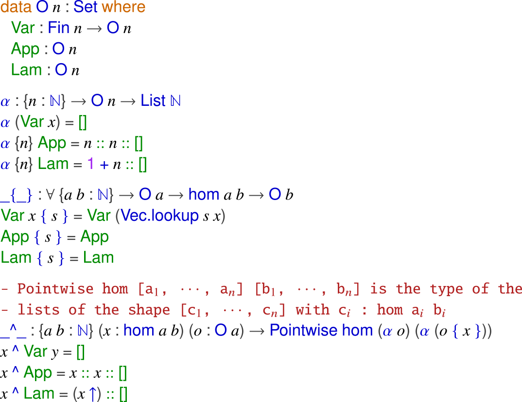


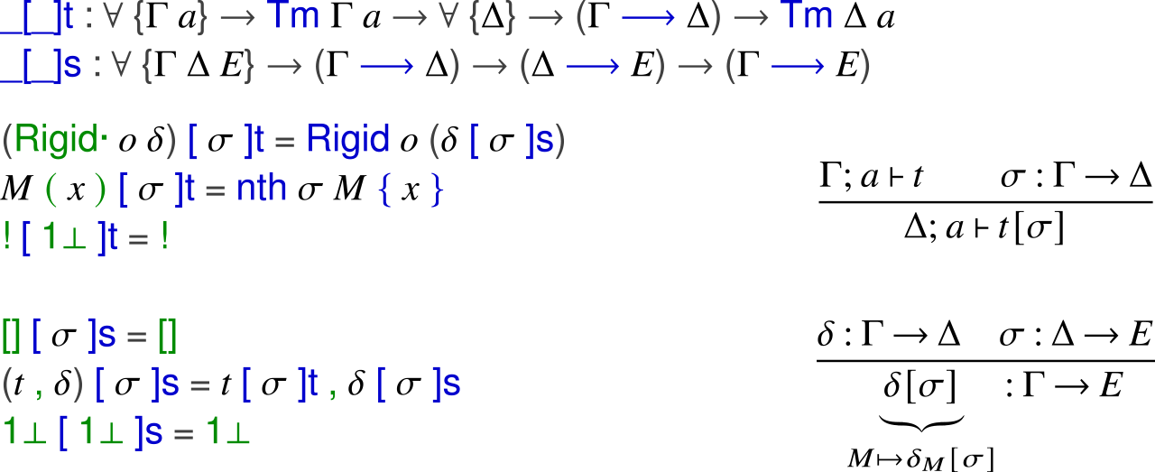
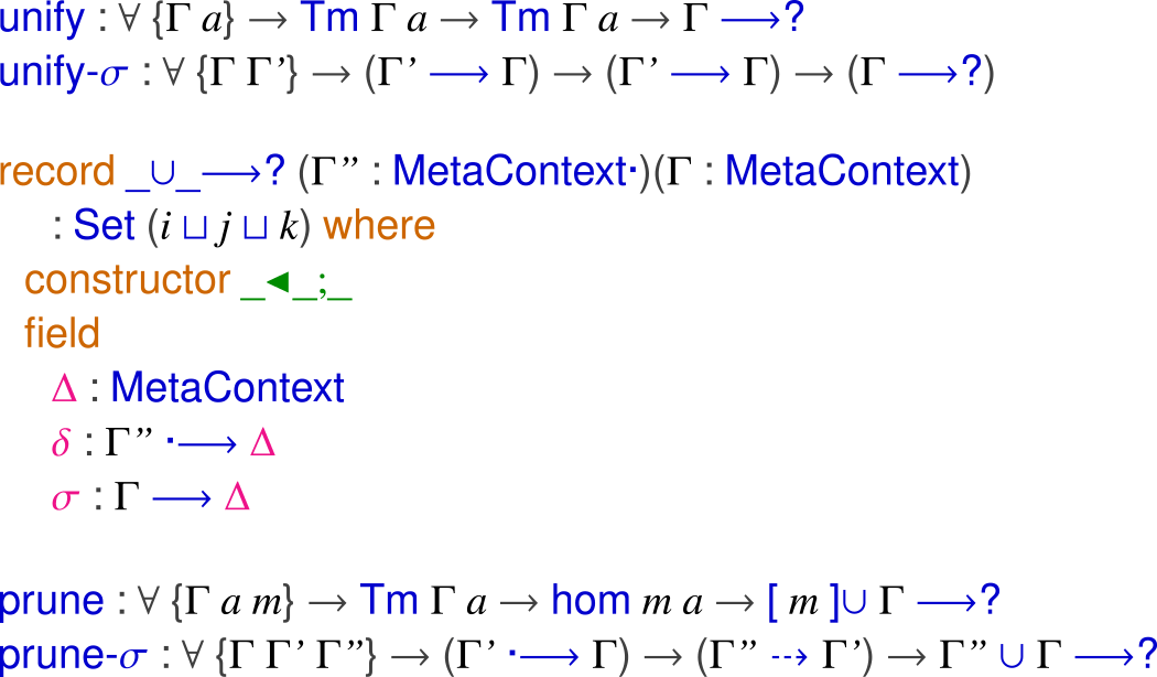
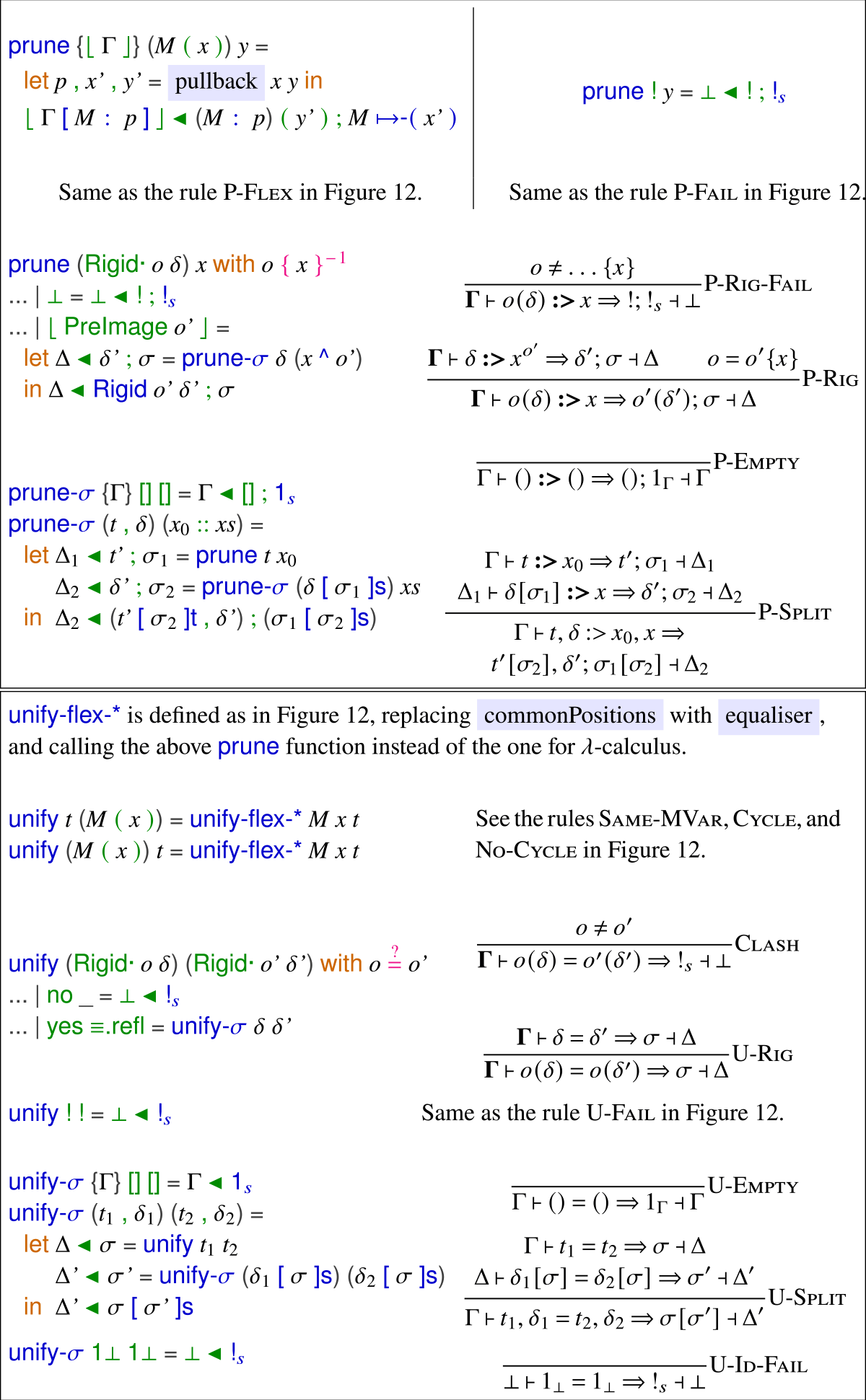


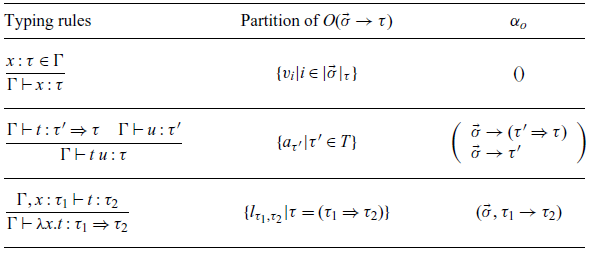

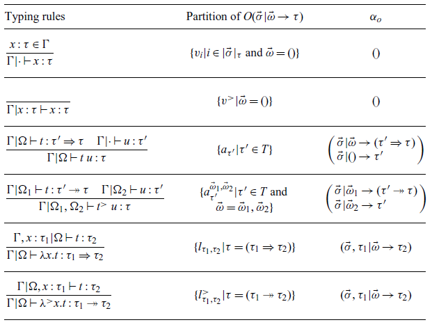


 Open access
Discussions
No Discussions have been published for this article.