




1 Introduction
In the past 10 years, research on totally disconnected, locally compact (t.d.l.c.) groups such as Willis [Reference Willis60] has increasingly focussed on their algorithmic aspects. We develop a general algorithmic theory of t.d.l.c. groups. This establishes a theoretical framework, and also enables us to prove non-computability results, such as the existence of an algorithmically t.d.l.c. group with a non-computable scale function.
In this article we assume that all topological groups have a countable basis. Our theory will address the following.
Questions 1.1.
-
(a) How can one define a computable presentation of a t.d.l.c. group?
-
(b) Which t.d.l.c. groups have such a presentation?
-
(c) Given a computable presentation, which associated objects (such as the rational valued Haar measures) are computable?
-
(d) Which constructions that lead from given to new t.d.l.c. groups have algorithmic versions?
-
(e) When is a computable presentation of a t.d.l.c. group unique up to computable isomorphism?
We begin with an informal summary of our main results, and the extent to which they answer these questions. Then we proceed to some background on t.d.l.c. groups and on computability. We will discuss the five questions and results answering them in more detail in the corresponding Sections 1.4–1.8 of the introduction.
1.1 Informal summary of answers to the questions
(a) We will introduce two approaches to defining a computable presentation of a t.d.l.c. group. Each of them addresses, in different ways, the problem that the domain is generally uncountable. One approach, which we call Baire presentation, employs computation based on approximations, as is done in the field of computable analysis. The other approach uses a duality between t.d.l.c. groups and certain countable structures we call meet groupoids. We will show that the two approaches are equivalent, in the sense that a group has a computable Baire presentation if, and only if, it has a computable presentation via its meet groupoid. This duality is a core technique towards answering the remaining questions. It also shows that Baire presentations can be “enhanced” to presentations as closed subgroups of
$S_\infty $
 : then the group operations are canonically computable, because they are given by the operations of composition and inverse on permutations of the natural numbers.
(b) Our thesis is that all “natural” countably based groups that are considered in the field of t.d.l.c. groups have computable presentations. We use our methods to collect evidence for this thesis. For instance, we show that the groups of the form
$\mathrm {PGL}_n(\mathbb Q_p)$
 are computable.
(c) Haar measure, modular function, and Cayley–Abels graphs (for the compactly generated case) are computable, while the scale function can fail to be computable.
(d) Many constructions of this sort have algorithmic versions. This is expected for constructions such as taking closed subgroups and forming local direct products. It is more surprising for taking quotients by closed normal subgroups, given that in the uncountable case there is no canonical set of coset representatives. The full power of the duality will be needed.
(e) While we stop short of giving a full answer to the question, we provide a criterion, based on the duality, of when a computable presentation of a t.d.l.c. group is unique up to computable isomorphism. We apply this to show that the split extension of
$\mathbb Q_p$
 by
${\mathbb {Z}}$
by
${\mathbb {Z}}$
 with the action of a generator given by
$x \mapsto xp$
with the action of a generator given by
$x \mapsto xp$
 has a unique computable presentation.
We hope that the first five sections of the article will be accessible to readers with only basic knowledge of computability theory; as we progress, we will explain some notions from computability theory that are more advanced.
Future work could use our framework to address the resource-bounded level, and even the practice of computation in t.d.l.c. groups. Several recent works study these topics for particular groups. We mention Conder [Reference Conder6, 4.1]: given a non-Archimedean local field K such as
${\mathbb {Q}}_p$
 , an algorithm is described to determine whether two input elements
$x,y$
, an algorithm is described to determine whether two input elements
$x,y$
 of
$\mathrm {SL}_2(K)$
of
$\mathrm {SL}_2(K)$
 (or
$\mathrm {PSL}_2(K)$
(or
$\mathrm {PSL}_2(K)$
 ) generate a discrete free subgroup. Conder subsequently discusses an implementation in the computer algebra system MAGMA. Such systems can only work with approximations to the elements in the uncountable domain. Thus, theoretical underpinning is needed for claims that such algorithms run efficiently. Future work could also explore the possibility to directly compute with the countable dual structure in computer algebra systems.
1.2 Background on t.d.l.c. groups
Van Dantzig [Reference Van Dantzig7] showed that each t.d.l.c. group has a neighbourhood basis of the identity consisting of compact open subgroups. With Question 1.1(a) in mind, we discuss some examples of t.d.l.c. groups. We will return to them repeatedly during the course of the article.
(i) All countable discrete groups and all profinite groups are t.d.l.c.
(ii)
$ ( \mathbb Q_p,+)$
 , the additive group of p-adic numbers for a prime p, is a t.d.l.c. group in neither of the two classes above.
(iii) The semidirect product
${\mathbb {Z}} \ltimes {\mathbb {Q}}_p$
 corresponding to the automorphism
$x \mapsto px$
corresponding to the automorphism
$x \mapsto px$
 on
${\mathbb {Q}}_p$
on
${\mathbb {Q}}_p$
 is t.d.l.c.
(iv) Algebraic groups over local fields, such as
$\operatorname {\mathrm {SL}}_n({\mathbb {Q}}_p)$
 for
$n \ge 2$
for
$n \ge 2$
 , are t.d.l.c.
(v) Given a connected countable undirected graph such that each vertex has finite degree, its automorphism group is t.d.l.c. The stabiliser of any vertex forms a compact open subgroup. By an undirected tree we mean a connected graph without cycles. For
$d \ge 3$
 , by
$T_d$
, by
$T_d$
 one denotes the undirected tree where each vertex has degree d. The group
$\mathrm {Aut}(T_d)$
one denotes the undirected tree where each vertex has degree d. The group
$\mathrm {Aut}(T_d)$
 was first studied by Tits [Reference Tits54].
Towards Question 1.1(b), we will review some objects that are associated with a locally compact group G.
1.2.1 Modular function.
The left and right Haar measures on G are treated in standard textbooks such as [Reference Hewitt and Ross17]. Recall that for any left Haar measure
$\mu $
 on G and any
$g \in G$
on G and any
$g \in G$
 , one obtains a further left Haar measure
$\mu _g$
, one obtains a further left Haar measure
$\mu _g$
 by defining
$\mu _g(A) = \mu (Ag)$
by defining
$\mu _g(A) = \mu (Ag)$
 . By the uniqueness up to a multiplicative constant of the left Haar measure, there is a real
$\Delta (g)>0 $
. By the uniqueness up to a multiplicative constant of the left Haar measure, there is a real
$\Delta (g)>0 $
 such that
$\mu _g(A) = \Delta (g) \mu (A)$
such that
$\mu _g(A) = \Delta (g) \mu (A)$
 for each measurable A. The function
$\Delta \colon G \to {\mathbb {R}}^+$
for each measurable A. The function
$\Delta \colon G \to {\mathbb {R}}^+$
 , called the modular function for G, is a group homomorphism.
1.2.2 Scale function.
Willis [Reference Willis58] introduced the scale function
$s \colon G \to {\mathbb {N}}^+$
 . Let
$g\in G$
. Let
$g\in G$
 . For a compact open subgroup V of G, let
$m(g,V) = |gVg^{-1}\colon V \cap gVg^{-1}| $
. For a compact open subgroup V of G, let
$m(g,V) = |gVg^{-1}\colon V \cap gVg^{-1}| $
 . Let
$s(g)$
. Let
$s(g)$
 be the minimum value of
$m(g,V)$
be the minimum value of
$m(g,V)$
 over all V. It is not hard to show that
$\Delta (g) = s(g)/s(g^{-1})$
over all V. It is not hard to show that
$\Delta (g) = s(g)/s(g^{-1})$
 . If a group has a normal compact open subgroup, as for Examples (i)–(iii) above, the scale function is constant of value 1. The group
${\mathbb {Z}} \ltimes {\mathbb {Q}}_p $
. If a group has a normal compact open subgroup, as for Examples (i)–(iii) above, the scale function is constant of value 1. The group
${\mathbb {Z}} \ltimes {\mathbb {Q}}_p $
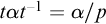
 for a prime p is among the simplest examples of a t.d.l.c. group with a nontrivial scale function:
$s(t)=p$
for a prime p is among the simplest examples of a t.d.l.c. group with a nontrivial scale function:
$s(t)=p$
 for the generator t of
${\mathbb {Z}}$
for the generator t of
${\mathbb {Z}}$
 such that
$ t \alpha t^{-1} = \alpha /p$
such that
$ t \alpha t^{-1} = \alpha /p$
 for each
$\alpha \in {\mathbb {Q}}_p$
for each
$\alpha \in {\mathbb {Q}}_p$
 .
.
1.2.3 Cayley–Abels graphs.
We first discuss a guiding principle in the study of a t.d.l.c. group G: it has a topological aspect that captures the small-scale (or local) behaviour, and a geometric aspect that captures the large-scale (or global) behaviour. The small-scale aspect is given by a compact open subgroup U (provided by van Dantzig’s theorem). Note that any two such subgroups are commensurable.
For the large-scale aspect, recall that in the discrete setting, Gromov and others initiated a geometric theory of finitely generated groups via their Cayley graphs. Given two generating sets, the corresponding graphs are quasi-isometric: there is a map
$\phi $
 from one vertex set to the other that only distorts distances affinely, and for some constant c, each vertex has at most distance c from the range of
$\phi $
from one vertex set to the other that only distorts distances affinely, and for some constant c, each vertex has at most distance c from the range of
$\phi $
 . For a t.d.l.c. group G, the generalisation of being f.g. is being algebraically generated by a compact subset. Given such a group G and a compact open subgroup U, note that G is algebraically generated by
$U \cup S$
. For a t.d.l.c. group G, the generalisation of being f.g. is being algebraically generated by a compact subset. Given such a group G and a compact open subgroup U, note that G is algebraically generated by
$U \cup S$
 for some finite set S closed under inversion. The Cayley–Abels graph
$\Gamma _{U,S}$
for some finite set S closed under inversion. The Cayley–Abels graph
$\Gamma _{U,S}$
 (see, e.g., Krön and Möller [Reference Krön and Möller24, Definition 3]) is a graph on the left cosets of U generalising the Cayley graph for discrete G (where one can take
$U= \{ e\}$
(see, e.g., Krön and Möller [Reference Krön and Möller24, Definition 3]) is a graph on the left cosets of U generalising the Cayley graph for discrete G (where one can take
$U= \{ e\}$
 ). As in the discrete case, any two such graphs for the same group are quasi-isometric. So, one can think of any Cayley–Abels graph as capturing the large-scale aspect of a compactly generated group.
Wesolek [Reference Wesolek57] provides further background and references on the topics discussed above. Also see the record of the 2022 conference on computational aspects of t.d.l.c. groups in Newcastle, Australia.
The following will be needed in several places.
Remark 1.2. The open mapping theorem for Hausdorff groups says that every surjective continuous homomorphism from a
$\sigma $
 -compact group G onto a Baire group H is open. This applies in particular when
$G,H$
-compact group G onto a Baire group H is open. This applies in particular when
$G,H$
 are countably based t.d.l.c. groups.
1.3 Background on computable mathematics
A general goal of computable mathematics is to study the algorithmic content of areas such as algebra [Reference Ash and Knight1, Reference Ershov and Goncharov10], analysis [Reference Pour-El and Richards46, Reference Weihrauch55], or topology [Reference Schröder50]. A first step is invariably to define what a computable presentation of a mathematical structure in that area is, such as a countable group, a complete metric space, or a separable Banach space. (Note that “computable” is the commonly accepted adjective used with presentations, rather than “algorithmic.”) One also introduces and studies computability for objects related to the structure. For instance, in computable analysis one uses rational approximations to reals in order to define what it means for a function
$f \colon \mathbb R \to \mathbb R$
 to be computable (see below for further details). A large body of results addresses the algorithmic content of classical results. There are also interesting new questions with no pendant in the classical setting. What is the complexity of recognizing that two computable presentations present the same structure? How hard is it to determine whether the structure presented has a certain property? (For instance, determine whether a computably presented group is torsion-free.) The basic distinction is “decidable/undecidable.” Mathematical logic provides a bevy of descriptive complexity classes, with corresponding completeness notions, for a more detailed answer in the undecidable case. For instance, torsion-freeness is of maximum complexity within the co-recursively enumerable properties.
Towards defining computable presentations, we first recall the definition of a computable function on natural numbers, slightly adapted to our purposes in that we allow the domain not only
${\mathbb {N}}^k$
 but also any computable subset of
${\mathbb {N}}^k$
but also any computable subset of
${\mathbb {N}}^k$
 .
.
Definition 1.3. Given a set
$S \subseteq {\mathbb {N}}^k$
 , where
$k\ge 1$
, where
$k\ge 1$
 , a function
$f \colon S \to {\mathbb {N}}$
, a function
$f \colon S \to {\mathbb {N}}$
 is called computable if there is a Turing machine that on inputs
$n_1, \ldots , n_k $
is called computable if there is a Turing machine that on inputs
$n_1, \ldots , n_k $
 decides whether the tuple of inputs
$(n_1, \ldots , n_k) $
decides whether the tuple of inputs
$(n_1, \ldots , n_k) $
 is in S, and if so outputs
$f(n_1, \ldots , n_k)$
is in S, and if so outputs
$f(n_1, \ldots , n_k)$
 . We say that S is computable if the function with domain S and constant value
$0$
. We say that S is computable if the function with domain S and constant value
$0$
 is computable.
One version of the Church–Turing thesis states that computability in this sense is the same as being computable by some algorithm. We note that without the restriction that the TM can decide membership in S, the function is called partial computable. The domain of a partial computable function is a recursively enumerable (r.e.) relation.
A structure in the model theoretic sense consists of a nonempty set D, called the domain, with relations and functions defined on it. The following definition was first formulated in the 1960s by Mal’cev [Reference Mal’cev27] and Rabin [Reference Rabin47], independently.
Definition 1.4. A computable structure is a structure such that the domain is a computable set
$D\subseteq {\mathbb {N}}$
 , and the functions and relations of the structure are computable. A countable structure S is called computably presentable if some computable structure W is isomorphic to it. In this context we call W a computable copy of S.
Next, we discuss how to define that an uncountable structure has a computable presentation. In the field of computable analysis, one represents all the elements of the structure by “names” which are directly accessible to computation, and requires that the functions and relations are computable on the names. For details see, e.g., Pauly [Reference Pauly43] or Schröder [Reference Schröder50]. Names usually are elements of the set
$[T]$
 of infinite paths on some computable subtree T of
${\mathbb {N}}^*$
of infinite paths on some computable subtree T of
${\mathbb {N}}^*$
 , the tree of strings with natural number entries. (Henceforth all paths will be infinite paths on rooted trees, starting at the root.) For instance, a standard name of a real number r is a path coding a sequence of rationals
${\langle {q_n}\rangle } _{n\in {\mathbb {N}}}$
, the tree of strings with natural number entries. (Henceforth all paths will be infinite paths on rooted trees, starting at the root.) For instance, a standard name of a real number r is a path coding a sequence of rationals
${\langle {q_n}\rangle } _{n\in {\mathbb {N}}}$
 such that
$|q_n - q_{n+1}| \le 2^{-n}$
such that
$|q_n - q_{n+1}| \le 2^{-n}$
 and
$\lim _n q_n = r$
and
$\lim _n q_n = r$
 . Using so-called “oracle Turing machines,” one can define computability of functions on
$[T]$
. Using so-called “oracle Turing machines,” one can define computability of functions on
$[T]$
 ; we will provide detail in Section 6. This indirectly defines computability on spaces relevant to computable analysis; for instance, one can define that a function on
${\mathbb {R}}$
; we will provide detail in Section 6. This indirectly defines computability on spaces relevant to computable analysis; for instance, one can define that a function on
${\mathbb {R}}$
 is computable. The example above shows that names and the object they denote can be of quite a different kind. In contrast, each totally disconnected Polish space is homeomorphic to
$[T]$
is computable. The example above shows that names and the object they denote can be of quite a different kind. In contrast, each totally disconnected Polish space is homeomorphic to
$[T]$
 for some subtree T of
${\mathbb {N}}^*$
for some subtree T of
${\mathbb {N}}^*$
 , which is advantageous because in principle there is no need to distinguish between names and objects in our setting.
An ad hoc way to define computability often works for particular classes of uncountable structures: impose algorithmic constraints on the definition of the class. For instance, the following is due to La Roche [Reference La Roche49] and Smith [Reference Smith52].
Definition 1.5. A profinite group G is computable if
$G= \varprojlim _i (A_i, \psi _i)$
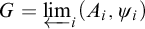 for a computable diagram
$ (A_i, \psi _i)_{i\in {\mathbb {N}}}$
for a computable diagram
$ (A_i, \psi _i)_{i\in {\mathbb {N}}}$
 of finite groups and epimorphisms
$\psi _i \colon A_i \to A_{i-1}$
of finite groups and epimorphisms
$\psi _i \colon A_i \to A_{i-1}$
 (
$i>0$
(
$i>0$
 ).
).
The aforementioned approach to profinite groups of Smith and la Roche admits equivalent formulations that work beyond this class. One such reformulation, in terms of effectively branching subtrees of
${\mathbb {N}}^*$
 , already is in Smith [Reference Smith52]. For the other, in terms of computably compact metric spaces, see Theorem 4.33 of the recent work [Reference Downey and Melnikov8]. Results of this sort indicate that the respective notion of computable presentability is robust for the class.
The remainder of the introduction discusses the questions posed at the beginning of the article in more detail.
1.4 Computable presentations of t.d.l.c. groups
We aim at a robust definition of the class of (countably based) t.d.l.c. groups with a computable presentation. We want this class to have good algorithmic closure properties, and also ask that our definition extend the existing definitions for discrete, and for profinite groups. We provide three types of computable presentations: type S and the more general type B are based on computation with approximations, while the separate type M is based on a reduction to countable structures via a duality. They will all turn out to be equivalent: a t.d.l.c. group has a computable presentation of one type iff it has one of the other type. The equivalences are algorithmically uniform.
Type S (for “symmetric group”) is based on the fact that each t.d.l.c. group G is isomorphic to a closed subgroup of
$S_\infty $
 . We represent such subgroups by subtrees of
${\mathbb {N}}^*$
. We represent such subgroups by subtrees of
${\mathbb {N}}^*$
 in a particular way to be described below. We impose algorithmic conditions on the tree to define when the presentation is computable. This approach is consistent with earlier work [Reference Greenberg, Melnikov, Nies and Turetsky16] on computable subgroups of
$S_\infty $
in a particular way to be described below. We impose algorithmic conditions on the tree to define when the presentation is computable. This approach is consistent with earlier work [Reference Greenberg, Melnikov, Nies and Turetsky16] on computable subgroups of
$S_\infty $
 .
.
Type M (for “meet groupoid”) is based on an algebraic structure
$\mathcal {W}(G)$
 on the countable set of compact open cosets in G. (Note here that every left coset
$A= gU$
on the countable set of compact open cosets in G. (Note here that every left coset
$A= gU$
 of a subgroup U is a right coset of the conjugate subgroup
$V= gUg^{-1}$
of a subgroup U is a right coset of the conjugate subgroup
$V= gUg^{-1}$
 , namely,
$A= Vg$
, namely,
$A= Vg$
 .) This structure is a partially ordered groupoid, with the usual set inclusion and multiplication of a left coset of a subgroup U with a right coset of U. The intersection of two compact open cosets is such a coset itself, unless it is empty. So, after adjoining
$\emptyset $
.) This structure is a partially ordered groupoid, with the usual set inclusion and multiplication of a left coset of a subgroup U with a right coset of U. The intersection of two compact open cosets is such a coset itself, unless it is empty. So, after adjoining
$\emptyset $
 as a least element (which only interacts trivially with the groupoid structure), we obtain a meet semilattice. A Type M computable presentation of G is a computable copy of the meet groupoid of G such that the index function on compact open subgroups, namely
$U,V \mapsto | U \colon U \cap V|$
as a least element (which only interacts trivially with the groupoid structure), we obtain a meet semilattice. A Type M computable presentation of G is a computable copy of the meet groupoid of G such that the index function on compact open subgroups, namely
$U,V \mapsto | U \colon U \cap V|$
 , is also computable. The idea to study appropriate Polish groups via an algebraic structure on their open cosets appeared in [Reference Kechris, Nies and Tent23], and was further elaborated in a paper on the complexity of the isomorphism problem for oligomorphic groups [Reference Nies, Schlicht and Tent42]. There, approximation structures called “coarse groups” are used that are given by the ternary relation “
$AB \subseteq C$
, is also computable. The idea to study appropriate Polish groups via an algebraic structure on their open cosets appeared in [Reference Kechris, Nies and Tent23], and was further elaborated in a paper on the complexity of the isomorphism problem for oligomorphic groups [Reference Nies, Schlicht and Tent42]. There, approximation structures called “coarse groups” are used that are given by the ternary relation “
$AB \subseteq C$
 ,” where
$A,B,C$
,” where
$A,B,C$
 are certain open cosets. In the present work, it will be important that we have explicit access to the combination of the groupoid and the meet semilattice structures (which coarse groups fail to provide). As a further example of the usefulness of meet groupoids, in Proposition 5.7 we will show that the meet groupoid of G can be used to understand the topological group of continuous automorphisms of G.
Type B (for “Baire”) of computable presentation generalizes Type S. For computable Baire presentations, one asks that the domain of G is what we call a computably locally compact (c.l.c.) subtree of
${\mathbb {N}}^*$
 (the tree of strings with natural number entries), and the operations are computable in the sense of oracle Turing machines. This generalizes the approach in [Reference Smith52] from profinite groups to t.d.l.c. groups. However, it also works for t.d.l.c. structures other than groups. We postpone this approach until Section 7, because it requires more advanced notions from computability theory. In particular, it relies on computable functions on the set of paths of a computable tree. These notions will be provided in Section 6. We note that Block and Miller [Reference Block and Miller2, Definition 1.1] have recently studied representations of general zero-dimensional functional structures via path spaces of trees.
Among our main results is that the various approaches to computable presentations are equivalent. This will be stated formally in Theorem 5.1 and its extension Theorem 7.6. Indeed, the approaches are equivalent in the strong sense that from a presentation of one type, one can effectively obtain a presentation of the other type for the same t.d.l.c. group. Below, we will initially say that a t.d.l.c. group is computably t.d.l.c. of a particular type, for instance via a closed subgroup of
$S_\infty $
 , or via a Baire presentation. Once the equivalences have been established, we will often omit this. These results suggest that our approach to computability for t.d.l.c. groups is natural and robust. We will later support this thesis with examples that show that many widely studied t.d.l.c. groups are computably t.d.l.c. Evidence for the robustness is also given in [Reference Melnikov and Ng34, Theorem 1.2], where it is shown that the notion of computable presentability for general locally compact Polish groups in their Definition 2.16 restricts to our notion in the totally disconnected case.
Baire presentations appear to be the simplest and most elegant notion of computable presentation for general totally disconnected Polish groups. However, computable Baire presentations are hard to study because the domain is usually uncountable (while the meet groupoids are countable), and there are no specific combinatorial tools available (unlike the case of permutations of
${\mathbb {N}}$
 ). In the proofs of several results, notably Theorem 9.9, we will work around this by replacing a Baire presentation by a more accessible presentation of Type M or S.
The operation that leads from a t.d.l.c. group to its meet groupoid has an inverse operation. Both operations are functorial for the categories with isomorphisms. This yields a duality between t.d.l.c. groups and a certain class of countable meet groupoids (similar to the duality in [Reference Nies, Schlicht and Tent42] between oligomorphic groups and the “coarse groups”). This class of meet groupoids can be described axiomatically. The equivalence of computable presentations of Types B and M can be extended to a computable version of that duality. We will elaborate on this in Remark 10.5.
1.5 Which t.d.l.c. groups G have computable presentations?
Discrete groups, as well as profinite groups, have a computable presentation as t.d.l.c. groups if and only if they have one in the previously established senses of Definitions 1.3 and 1.5, respectively. For discrete groups this will be shown in Example 4.8; for profinite groups it will be obtained by combining Propositions 7.3 and B.7. We provide several examples of computable presentations for t.d.l.c. groups outside these two classes. The various equivalent approaches to computable presentations will be useful for this, because they allow us to construct a presentation of the type most appropriate for a given group. For a group of automorphisms such as
${Aut}(T_d)$
 , we use Type S (presentations as closed subgroups of
$S_\infty $
, we use Type S (presentations as closed subgroups of
$S_\infty $
 ). For
$({\mathbb {Q}}_p, + )$
). For
$({\mathbb {Q}}_p, + )$
 , we use Type M (meet groupoids). For
$\operatorname {\mathrm {SL}}_n({\mathbb {Q}}_p)$
, we use Type M (meet groupoids). For
$\operatorname {\mathrm {SL}}_n({\mathbb {Q}}_p)$
 , we use Type B (computable Baire presentations). The first author has shown how to give an equivalent definition of a computable t.d.l.c. group in terms of an ‘effectively
$\sigma $
, we use Type B (computable Baire presentations). The first author has shown how to give an equivalent definition of a computable t.d.l.c. group in terms of an ‘effectively
$\sigma $
 -compact metric’. Using this one can generalize the latter example to other algebraic groups over
${\mathbb {Q}}_p$
-compact metric’. Using this one can generalize the latter example to other algebraic groups over
${\mathbb {Q}}_p$
 . For an outline of this work, see [Reference Nies39, Section 4]. Neretin’s groups
$\mathcal {N}_d$
. For an outline of this work, see [Reference Nies39, Section 4]. Neretin’s groups
$\mathcal {N}_d$
 of almost automorphisms of
$T_d$
of almost automorphisms of
$T_d$
 , for
$d \ge 3$
, for
$d \ge 3$
 [Reference Kapoudjian21], are computable by upcoming work of Ferov, Skipper, and Willis.
1.6 Associated computable objects.
Recall that to a t.d.l.c. group G we associate its meet groupoid
$\mathcal {W}(G)$
 , an algebraic structure on its compact open cosets. If G is given by a computable Baire presentation, then we construct a copy
$\mathcal {W} = \mathcal {W}_{\text {comp}}(G)$
, an algebraic structure on its compact open cosets. If G is given by a computable Baire presentation, then we construct a copy
$\mathcal {W} = \mathcal {W}_{\text {comp}}(G)$
 that is computable in a strong sense, essentially including the condition that some (and hence any) rational valued Haar measure on G is computable when restricted to a function
$\mathcal {W} \to {\mathbb {R}}$
that is computable in a strong sense, essentially including the condition that some (and hence any) rational valued Haar measure on G is computable when restricted to a function
$\mathcal {W} \to {\mathbb {R}}$
 . We will show in Theorem 8.2 that the left, and hence also the right, action of G on
$\mathcal {W}$
. We will show in Theorem 8.2 that the left, and hence also the right, action of G on
$\mathcal {W}$
 is computable. We conclude that the modular function on G is computable.
If G is compactly generated, for each Cayley–Abels graph one can determine a computable copy, and any two copies of this type are computably quasi-isometric (Theorem 8.5). Intuitively, this means that the large-scale structure of G is a computable invariant.
Assertions that the scale function is computable have been made for particular t.d.l.c. groups in works such as Glöckner [Reference Glöckner14] and Willis [Reference Willis59, Section 6]; see the survey [Reference Willis60]. In these particular cases, it was generally clear what it means that one can compute the scale
$s(g)$
 : provide an algorithm that shows it. One has to declare what kind of input the algorithm takes; necessarily it has to be some approximation to g, as g ranges over a potentially uncountable domain. Our new framework allows us to give a precise meaning to the question whether the scale function is computable for a particular computable presentation of a t.d.l.c. group, thus also allowing for a negative answer. In Theorem A.1, which is joint with George Willis, we provide a computable presentation of a t.d.l.c. group G such that the scale function fails to be computable for this presentation.
It remains open whether for some computably presented t.d.l.c. group G, the scale is non-computable for each of its computable presentations. An even stronger negative result would be that such a G can be chosen to have a unique computable presentation (see the discussion in Section 1.8 below).
1.7 Algorithmic versions of constructions that lead from given to new t.d.l.c. groups.
Section 9 shows that for many constructions that have been studied in the theory of t.d.l.c. groups, the class of computably t.d.l.c. groups is closed under suitable algorithmic versions. In particular, the constructions (1)–(3) and (6) described in Wesolek [Reference Wesolek56, Theorem 1.3] can be phrased algorithmically in such a way that they stay within the class of computably t.d.l.c. groups; this provides further evidence that our class is robust. These constructions are suitable versions, in our algorithmic topological setting, of passing to closed subgroups, taking group extensions via continuous actions, forming “local” direct products, and taking quotients by closed normal subgroups (see [Reference Wesolek56, Section 2] for details on these constructions). The algorithmic version of taking quotients (Theorem 9.9) is the most demanding; it uses extra insights, provided in Theorem 8.2, from the proofs that the various forms of computable presentation are equivalent.
Several constructions lead to new examples of t.d.l.c. groups with computable presentations. For instance, after defining a computable presentation of
$\operatorname {\mathrm {SL}}_{n+1}({\mathbb {Q}}_p)$
 (
$n \ge 2$
(
$n \ge 2$
 , p a prime) directly in Proposition 7.8, we proceed to a computable presentation of
$\operatorname {\mathrm {GL}}_n({\mathbb {Q}}_p)$
, p a prime) directly in Proposition 7.8, we proceed to a computable presentation of
$\operatorname {\mathrm {GL}}_n({\mathbb {Q}}_p)$
 via taking a closed subgroup, and then to
$\operatorname {\mathrm {PGL}}_n({\mathbb {Q}}_p)$
via taking a closed subgroup, and then to
$\operatorname {\mathrm {PGL}}_n({\mathbb {Q}}_p)$
 via taking the quotient by the centre.
1.8 When is a computable presentation unique?
Citing Willis, [Reference Willis60, Section 5], “it is a truism that computation in a group depends on the description of the group.” In the present article, we apply our notion of computable presentability of a t.d.l.c. group to give a formal version of this statement. We also give some examples where the general statement fails. Viewing a computable Baire presentation as a description, we are interested in the question whether such a description is unique, in the sense that between any two of them there is a computable isomorphism. Adapting terminology for countable structures going back to Mal’cev (see below), we will call such a group autostable. If a t.d.l.c. group is autostable, then computation in the group can be seen as independent of its particular description.
Criterion 10.2 reduces the problem of whether a t.d.l.c. group is autostable to the similar problem in the countable setting of meet groupoids. We apply it to show that
$({\mathbb {Q}}_p, +)$
 is autostable, and so is
${\mathbb {Z}} \ltimes {\mathbb {Q}}_p $
is autostable, and so is
${\mathbb {Z}} \ltimes {\mathbb {Q}}_p $
 . Proving the autostability of these groups requires more effort than the reader would perhaps expect. For other groups, such as
$\operatorname {\mathrm {SL}}_n({\mathbb {Q}}_p)$
. Proving the autostability of these groups requires more effort than the reader would perhaps expect. For other groups, such as
$\operatorname {\mathrm {SL}}_n({\mathbb {Q}}_p)$
 for
$n \ge 2$
for
$n \ge 2$
 and
${Aut}(T_d)$
and
${Aut}(T_d)$
 , we leave open whether a computable presentation is unique up to computable isomorphism.
1.9 Some context.
1.9.1 Related work on autostability.
A countable structure is called autostable (or computably categorical) [Reference Ash and Knight1, Reference Ershov and Goncharov10] if it has a computable copy, and such a copy is unique up to computable isomorphism. For example, any computable finitely generated algebraic structure is autostable because any homomorphism
$A \to B$
 for such structures
$A,B$
for such structures
$A,B$
 can be reconstructed from the images of generators of A, and is therefore computable. In contrast, there is a discrete 2-step nilpotent group with exactly two computable presentations up to computable isomorphism [Reference Goncharov15]. For t.d.l.c. groups, in the discrete case our notion of autostability reduces to the established one.
A profinite abelian group is autostable if and only if its Pontryagin dual is autostable ([Reference Melnikov31]; also see [Reference Downey and Melnikov9, Theorem 9.5.7]). Note that this dual is a discrete, torsion abelian group. Autostability of the latter type of groups is characterized in [Reference Melnikov and Ng33]. In this way one obtains a characterization of autostability for profinite abelian groups.
Pour El and Richards [Reference Pour-El and Richards46] gave an example of a Banach space with two computable presentations so that there is no computable linear isometry between them. Works such as [Reference Melnikov30] and then [Reference Clanin, McNicholl and Stull5, Reference Iljazović19, Reference McNicholl29] systematically study autostability in separable spaces, using tools of computable (discrete) algebra.
1.9.2 Other related work.
Our work with Lupini [Reference Lupini, Melnikov and Nies26] focusses on abelian locally compact groups. We introduce two notions of computable presentation for abelian t.d.l.c. groups that take into account their specific structural properties: The first is based on the fact that such groups are pro-countable, the other on the fact that such a group is an extension of a discrete group by a profinite group. Both notions can be used to provide examples of computable abelian t.d.l.c. groups that are neither discrete nor compact. The same work [Reference Lupini, Melnikov and Nies26] states that in the abelian case, the notion of computable presentability given in the present article is equivalent to these notions, referring to the present article. We prove this in Appendix B.
An approach to computability for Polish groups was suggested in Melnikov and Montalbán [Reference Melnikov and Montalbán32] and then developed in, e.g., Melnikov [Reference Melnikov31], Pauly et al. [Reference Pauly, Seon, Ziegler, Fernández and Muscholl44], and the aforementioned Melnikov and Ng [Reference Melnikov and Ng34]. In that approach, a Polish group is said to be computable if the underlying topological space is computably, completely metrized and the group operations are computable operators (functionals) on this space. By [Reference Melnikov31, Corollary 1.6] there is computably metrized profinite group that does not possess a computable presentation in the sense of Definition 1.5. However, if we additionally assume that the underlying computably metrized space is ‘computably compact’ (equivalently, the Haar measure is computable [Reference Pauly, Seon, Ziegler, Fernández and Muscholl44]), then we can produce a computable presentation of the group in that sense (see Downey and Melnikov [Reference Downey and Melnikov8] for a proof).
Nies and Schlicht [Reference Nies and Schlicht41, Section 4] study a Borel duality of classes of groups closed subgroups of
$S_\infty $
 with meet groupoids in an axiomatic setting, which encompasses the class of locally Roelcke precompact groups, much larger than the class of t.d.l.c. groups. It would be interesting to probe the computable content of this theory. The present authors [Reference Melnikov and Nies35, Section 6] study the Chabauty space of a computably t.d.l.c. group G via its meet groupoid
$\mathcal {W}(G)$
with meet groupoids in an axiomatic setting, which encompasses the class of locally Roelcke precompact groups, much larger than the class of t.d.l.c. groups. It would be interesting to probe the computable content of this theory. The present authors [Reference Melnikov and Nies35, Section 6] study the Chabauty space of a computably t.d.l.c. group G via its meet groupoid
$\mathcal {W}(G)$
 ; in particular, they characterise the computably closed subgroups of G via certain computable ideals of
$\mathcal {W}(G)$
; in particular, they characterise the computably closed subgroups of G via certain computable ideals of
$\mathcal {W}(G)$
 . Ferov et al. [Reference Ferov, Tornier and Willis11] survey algorithmic aspects of particular t.d.l.c. groups. They connect to the present article, and also discuss practical implementations on computer algebra systems.
2 Computably locally compact subtrees of
${\mathbb {N}}^*$
 .
.

Definition 2.4 of this section introduces c.l.c. trees. This purely computability-theoretic concept will matter for the whole article. For basics on computability theory see, e.g., the first two chapters of [Reference Soare53], or the first chapter of [Reference Nies37] which also contains notation on strings and trees. Our article is mostly consistent with the terminology of these two sources. They also serve for basic concepts such as Turing programs, computable functions, as well as partial computable (or partial recursive) functions, which will be needed from Section 6 onwards. In this section we will review some more specialized concepts related to computability.
Notation 2.1. Let
${\mathbb {N}}^*$
 denote the set of strings with natural numbers as entries. We use letters
$\sigma , \tau , \rho ,$
denote the set of strings with natural numbers as entries. We use letters
$\sigma , \tau , \rho ,$
 etc., for elements of
${\mathbb {N}}^*$
etc., for elements of
${\mathbb {N}}^*$
 . The set
${\mathbb {N}}^*$
. The set
${\mathbb {N}}^*$
 can be seen as a directed tree: the empty string is the root, and the successor relation is given by appending a number at the end of a string. One writes
$\sigma \preceq \tau $
can be seen as a directed tree: the empty string is the root, and the successor relation is given by appending a number at the end of a string. One writes
$\sigma \preceq \tau $
 to denote that
$\sigma $
to denote that
$\sigma $
 is an initial segment of
$\tau $
is an initial segment of
$\tau $
 , and
$\sigma \prec \tau $
, and
$\sigma \prec \tau $
 to denote that
$\sigma $
to denote that
$\sigma $
 is a proper initial segment. For
$k \le |\tau |$
is a proper initial segment. For
$k \le |\tau |$
 , by
$\tau \! \upharpoonright _{k}$
, by
$\tau \! \upharpoonright _{k}$
 one denotes the initial segment of
$\tau $
one denotes the initial segment of
$\tau $
 that has length k. We can also identify finite strings of length n+
$1$
that has length k. We can also identify finite strings of length n+
$1$
 with partial functions
${\mathbb {N}} \rightarrow {\mathbb {N}}$
with partial functions
${\mathbb {N}} \rightarrow {\mathbb {N}}$
 having finite support
$\{0, \ldots , n\}$
having finite support
$\{0, \ldots , n\}$
 . We then write
$\tau _i$
. We then write
$\tau _i$
 instead of
$\tau (i)$
instead of
$\tau (i)$
 . By
$\max (\tau )$
. By
$\max (\tau )$
 we denote
$\max \{\tau _i \colon \, i \le n\}$
we denote
$\max \{\tau _i \colon \, i \le n\}$
 . Let
$h \colon {\mathbb {N}}^* \to {\mathbb {N}}$
. Let
$h \colon {\mathbb {N}}^* \to {\mathbb {N}}$
 be the canonical encoding given by
$h(w)= \prod _{i< |w|} p_i^{w_i+1}$
be the canonical encoding given by
$h(w)= \prod _{i< |w|} p_i^{w_i+1}$
 , where
$w = (w_0, \ldots , w_{|w|-1})$
, where
$w = (w_0, \ldots , w_{|w|-1})$
 , and
$p_i$
, and
$p_i$
 is the i-th prime number. By convention
$h()=1$
is the i-th prime number. By convention
$h()=1$
 .
.
Definition 2.2 (Strong indices for finite sets of strings).
For a finite set
$u \subseteq {\mathbb {N}}^*$
 let
$n_u=\sum _{\eta \in u} 2^{h(\eta ) }$
let
$n_u=\sum _{\eta \in u} 2^{h(\eta ) }$
 ; one says that
$n_u$
; one says that
$n_u$
 is the strong index for u.
We will usually identify a finite subset of
$ {\mathbb {N}}^* $
 with its strong index.
Remark 2.3. Why “strong index”? In computability theory, by an index one usually means a (code for a) Turing program that decides a set or computes a function. Such an index can be obtained from a strong index as defined above. However, a strong index tells us more about the finite set, such as its size. This is not true for an index as a Turing program.
Unless otherwise mentioned, by a (rooted) tree we mean a nonempty subset T of
${\mathbb {N}}^*$
 such that
$(\sigma \in T \wedge \rho \prec \sigma ) \to \rho \in T$
such that
$(\sigma \in T \wedge \rho \prec \sigma ) \to \rho \in T$
 . For
$k \in {\mathbb {N}}$
. For
$k \in {\mathbb {N}}$
 we write

By
$[T] $
 one denotes the set of (infinite) paths of a tree T starting at the root. Our trees usually have no leaves, so
$[T]$
one denotes the set of (infinite) paths of a tree T starting at the root. Our trees usually have no leaves, so
$[T]$
 is a closed set in Baire space
${\mathbb {N}}^{\mathbb {N}}$
is a closed set in Baire space
${\mathbb {N}}^{\mathbb {N}}$
 equipped with the usual product topology. Note that
$[T]$
equipped with the usual product topology. Note that
$[T]$
 is compact if and only if each level of T is finite, in other words, iff T is finitely branching. For
$\sigma \in T$
is compact if and only if each level of T is finite, in other words, iff T is finitely branching. For
$\sigma \in T$
 , let
, let

That is,
$ [\sigma ]_T $
 is the cone of paths on T that extend
$\sigma $
is the cone of paths on T that extend
$\sigma $
 . One says that T is computable if the set
$\{h(\sigma ) \colon \, \sigma \in T \}$
. One says that T is computable if the set
$\{h(\sigma ) \colon \, \sigma \in T \}$
 is computable.
Definition 2.4 (Computably locally compact trees).
Let T be a computable subtree of
$ {\mathbb {N}}^*$
 without leaves. We say that T is c.l.c. if for some
$k \in {\mathbb {N}}$
without leaves. We say that T is c.l.c. if for some
$k \in {\mathbb {N}}$
 there is a computable function
$H \colon {\mathbb {N}}^k \times {\mathbb {N}} \to {\mathbb {N}} $
there is a computable function
$H \colon {\mathbb {N}}^k \times {\mathbb {N}} \to {\mathbb {N}} $
 such that

In particular, if
$\sigma \in T^{[\ge k]}$
 , then
$ \{ i \colon \sigma \hat {\ } i \in T\}$
, then
$ \{ i \colon \sigma \hat {\ } i \in T\}$
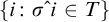 is finite.
Frequently we will have
$k=1$
 , so that only the root can have infinitely many successors. In this case the condition says that there is a computable function
$H \colon {\mathbb {N}} \times {\mathbb {N}} \to {\mathbb {N}}$
, so that only the root can have infinitely many successors. In this case the condition says that there is a computable function
$H \colon {\mathbb {N}} \times {\mathbb {N}} \to {\mathbb {N}}$
 such that
$\rho (i) \le H(\rho (0), i)$
such that
$\rho (i) \le H(\rho (0), i)$
 for each positive
$i< |\rho |$
for each positive
$i< |\rho |$
 .
.
Given a c.l.c. tree T, the compact open subsets of
$[T]$
 can be algorithmically encoded by natural numbers; the notation below will be used throughout.
Definition 2.5 (Code numbers for compact open sets).
Suppose that a tree T is c.l.c. via
$k\in {\mathbb {N}}$
 . For a finite set
$u\subseteq T^{\ge k}$
. For a finite set
$u\subseteq T^{\ge k}$
 , let
, let

By a code number for a compact open set
$\mathcal {K}\subseteq [T]$
 we mean the strong index for a finite set u of strings such that
$\mathcal {K} = \mathcal {K}_u$
we mean the strong index for a finite set u of strings such that
$\mathcal {K} = \mathcal {K}_u$
 .
.
Clearly, each compact open subset
$\mathcal {K}$
 of
$[T]$
of
$[T]$
 is of the form
$\mathcal {K}_u$
is of the form
$\mathcal {K}_u$
 for some u. Such a code number is not unique (unless
$\mathcal {K}$
for some u. Such a code number is not unique (unless
$\mathcal {K}$
 is empty). So we will need to distinguish between the actual compact open set, and any of its code numbers. Note that one can decide, given
$u \in {\mathbb {N}} $
is empty). So we will need to distinguish between the actual compact open set, and any of its code numbers. Note that one can decide, given
$u \in {\mathbb {N}} $
 as an input, whether u is a code number.
The following lemma shows that the basic set-theoretic relations and operations are decidable for sets of the form
$\mathcal {K}_u$
 , similar to the case of finite subsets of
${\mathbb {N}}$
, similar to the case of finite subsets of
${\mathbb {N}}$
 .
.
Lemma 2.6. Suppose a tree T is c.l.c. via
$k \in {\mathbb {N}}$
 . Given code numbers
$u, w$
. Given code numbers
$u, w$
 ,
,
-
(i) one can compute code numbers for $\mathcal {K}_u \cup \mathcal {K}_w$
and
$\mathcal {K}_u \cap \mathcal {K}_w$
; -
(ii) one can decide whether $\mathcal {K}_u \subseteq \mathcal {K}_w$
. So one can, given a code number
$u\in {\mathbb {N}}$
, compute the minimal code number
$u^*\in {\mathbb {N}}$
such that
$\mathcal {K}_{u^*}=\mathcal {K}_u$
.


Proof. (i) The case of union is trivial. For the intersection operation, it suffices to consider the case that u and w are singletons. For strings
$\alpha , \beta \in T$
 , one has
$[\alpha ]_T \cap [\beta ]_T = \emptyset $
, one has
$[\alpha ]_T \cap [\beta ]_T = \emptyset $
 if
$\alpha , \beta $
if
$\alpha , \beta $
 are incompatible, and otherwise
$[\alpha ]_T \cap [\beta ]_T = [\gamma ]_T$
are incompatible, and otherwise
$[\alpha ]_T \cap [\beta ]_T = [\gamma ]_T$
 where
$\gamma $
where
$\gamma $
 is the longest common initial segment of
$\alpha , \beta $
is the longest common initial segment of
$\alpha , \beta $
 .
.
(ii) Let H be a computable binary function as in Definition 2.4. It suffices to consider the case that u is a singleton. Suppose that
$\alpha \in T^{[\ge k]}$
 . The algorithm to decide whether
$[\alpha ]_T \subseteq \mathcal {K}_w$
. The algorithm to decide whether
$[\alpha ]_T \subseteq \mathcal {K}_w$
 is as follows. Let N be the maximum length of a string in w. Answer “yes” if for each
$\beta \succeq \alpha $
is as follows. Let N be the maximum length of a string in w. Answer “yes” if for each
$\beta \succeq \alpha $
 of length N such that
$\beta (i) \le H(\alpha \! \upharpoonright _{k}, k)$
of length N such that
$\beta (i) \le H(\alpha \! \upharpoonright _{k}, k)$
 for each
$i < N$
for each
$i < N$
 , there is
$\gamma \in w$
, there is
$\gamma \in w$
 such that
$\gamma \preceq \beta $
such that
$\gamma \preceq \beta $
 . Otherwise, answer “no.”
Definition 2.7. Given a c.l.c. tree T, let
$E_T$
 denote the set of minimal code numbers for compact open subsets of
$[T]$
denote the set of minimal code numbers for compact open subsets of
$[T]$
 . By the foregoing lemma,
$E_T$
. By the foregoing lemma,
$E_T$
 is decidable.
3 Defining computable t.d.l.c. groups via closed subgroups of
$S_\infty $
.

This section, in particular Definition 3.3, spells out Type S of computable presentations of t.d.l.c. groups, informally described in Section 1.4.
3.1 Computable closed subgroups of
$S_\infty $
.

We first provide a computable presentation of the group of permutations of
${\mathbb {N}}$
 . It is related to the computable presentation in [Reference Greenberg, Melnikov, Nies and Turetsky16, Definition 1.2], where the group is viewed as a topological group with a computable compatible metric. However, in our presentation, an element of the group is given as a path on a tree that encodes a pair
$(h, h^{-1})$
. It is related to the computable presentation in [Reference Greenberg, Melnikov, Nies and Turetsky16, Definition 1.2], where the group is viewed as a topological group with a computable compatible metric. However, in our presentation, an element of the group is given as a path on a tree that encodes a pair
$(h, h^{-1})$
 where h is a permutation of
${\mathbb {N}}$
where h is a permutation of
${\mathbb {N}}$
 . This enables us to define a computable tree, denoted
${Tree}(S_\infty ) $
. This enables us to define a computable tree, denoted
${Tree}(S_\infty ) $
 , each path of which corresponds to a permutation of
${\mathbb {N}}$
, each path of which corresponds to a permutation of
${\mathbb {N}}$
 .
.
Suppose strings
$\sigma _0, \sigma _1 \in {\mathbb {N}}^*$
 both have length N. By
$\sigma _0 \oplus \sigma _1$
both have length N. By
$\sigma _0 \oplus \sigma _1$
 we denote the string of length
$2N$
we denote the string of length
$2N$
 that alternates between
$\sigma _0$
that alternates between
$\sigma _0$
 and
$\sigma _1$
and
$\sigma _1$
 . That is,

Similarly, for functions
$f_0, f_1$
 on
${\mathbb {N}}$
on
${\mathbb {N}}$
 , we define a function
$f_0 \oplus f_1$
, we define a function
$f_0 \oplus f_1$
 on
${\mathbb {N}}$
on
${\mathbb {N}}$
 by
by

Informally,
${Tree}(S_\infty )$
 is the tree of strings such that it is consistent that the map given by the entries at odd positions extends to an inverse of the map given by entries at even positions. Formally, let
${Tree}(S_\infty ) =$
is the tree of strings such that it is consistent that the map given by the entries at odd positions extends to an inverse of the map given by entries at even positions. Formally, let
${Tree}(S_\infty ) =$


We view
$S_\infty $
 as a group on the set of paths of
${Tree}(S_\infty )$
as a group on the set of paths of
${Tree}(S_\infty )$
 . Its domain is the set of functions of the form
$ h\oplus h^{-1}$
. Its domain is the set of functions of the form
$ h\oplus h^{-1}$
 where h is a permutation of
${\mathbb {N}}$
where h is a permutation of
${\mathbb {N}}$
 ; if
$f= f_0 \oplus f_1$
; if
$f= f_0 \oplus f_1$
 and
$g= g_0 \oplus g_1$
and
$g= g_0 \oplus g_1$
 in
$ S_\infty $
in
$ S_\infty $
 , we define
$f^{-1} = f_1 \oplus f_0$
, we define
$f^{-1} = f_1 \oplus f_0$
 and
$g f = (g_0 \circ f_0) \oplus (f_1 \circ g_1 )$
and
$g f = (g_0 \circ f_0) \oplus (f_1 \circ g_1 )$
 . We will verify in Fact 6.6 below that these group operations are computable (in the sense of Definition 6.3).
Definition 3.1. We say that a closed subgroup C of
$S_\infty $
 is computable if its corresponding tree, namely
${Tree}(C)=\{\eta \in {Tree}(S_\infty ) \colon [\eta ]_T \cap C \neq \emptyset \},$
is computable if its corresponding tree, namely
${Tree}(C)=\{\eta \in {Tree}(S_\infty ) \colon [\eta ]_T \cap C \neq \emptyset \},$
 is computable.
Remark 3.2. It is well known that the closed subgroups of
$S_\infty $
 are precisely the automorphism groups of structures M with domain
${\mathbb {N}}$
are precisely the automorphism groups of structures M with domain
${\mathbb {N}}$
 . Suppose that M is a computable structure, and there is an algorithm to decide whether a bijection between finite subsets of M (encoded by a strong index) can be extended to an automorphism. Then the automorphism group of M is computable. To see this, one uses that a string
$\eta =\sigma \oplus \tau $
. Suppose that M is a computable structure, and there is an algorithm to decide whether a bijection between finite subsets of M (encoded by a strong index) can be extended to an automorphism. Then the automorphism group of M is computable. To see this, one uses that a string
$\eta =\sigma \oplus \tau $
 on
${Tree}(S_\infty )$
on
${Tree}(S_\infty )$
 determines the finite injective map

between finite subsets of M. This map is extendible to an automorphism of M if and only if
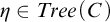
$\eta \in {Tree}(C)$
 .
.
For instance, assuming a computable bijection between
${\mathbb {Q}}$
 and
${\mathbb {N}}$
and
${\mathbb {N}}$
 , the group
$ C=\text {Aut}({\mathbb {Q}}, <)$
, the group
$ C=\text {Aut}({\mathbb {Q}}, <)$
 is computable: By Cantor’s back and forth argument, a bijection between finite subsets of
${\mathbb {Q}}$
is computable: By Cantor’s back and forth argument, a bijection between finite subsets of
${\mathbb {Q}}$
 can be extended to an automorphism of C if and only if it preserves the ordering. There is an algorithm to decide the latter condition.
3.2 First definition of computably t.d.l.c. groups.
If a subgroup C of
$S_\infty $
 is locally compact, then there is an
$n \in {\mathbb {N}}$
is locally compact, then there is an
$n \in {\mathbb {N}}$
 such that
$C\cap V_n$
such that
$C\cap V_n$
 is compact, where
$V_n$
is compact, where
$V_n$
 is the group of elements of
$S_\infty $
is the group of elements of
$S_\infty $
 fixing
$0, \ldots , n-1$
fixing
$0, \ldots , n-1$
 . Thus all the 1-orbits for the natural action of
$C\cap V_n$
. Thus all the 1-orbits for the natural action of
$C\cap V_n$
 on
${\mathbb {N}}$
on
${\mathbb {N}}$
 are finite, which implies that in
${Tree}(C) $
are finite, which implies that in
${Tree}(C) $
 each string of length at least
$2n$
each string of length at least
$2n$
 has only finitely many successors. This motivates the following definition.
Definition 3.3. Let G be a t.d.l.c. group. We say that G is computably t.d.l.c. (via a closed subgroup of
$S_\infty $
 ) if there is a closed subgroup C of
$S_\infty $
) if there is a closed subgroup C of
$S_\infty $
 such that
$G \cong C$
such that
$G \cong C$
 , and the tree

is c.l.c. in the sense of Definition 2.4.
In this context we will often ignore the difference between G and C. That is, we will assume that G itself is a closed subgroup of
$S_\infty $
 .
.
Recall from the introduction that
$\mathrm {Aut}(T_d)$
 is the group of automorphism of the undirected tree
$T_d$
is the group of automorphism of the undirected tree
$T_d$
 where each vertex has degree d.
Example 3.4. Let
$d\ge 3$
 . The t.d.l.c. group
$G=\text {Aut}(T_d)$
. The t.d.l.c. group
$G=\text {Aut}(T_d)$
 is computably t.d.l.c. via a closed subgroup of
$S_\infty $
is computably t.d.l.c. via a closed subgroup of
$S_\infty $
 .
.
Proof. Via an effective encoding of the vertices of
$T_d$
 by the natural numbers, we can view G itself as a closed subgroup of
$S_\infty $
by the natural numbers, we can view G itself as a closed subgroup of
$S_\infty $
 . A finite injection
$\alpha $
. A finite injection
$\alpha $
 on
$T_d$
on
$T_d$
 can be extended to an automorphism of
$T_d$
can be extended to an automorphism of
$T_d$
 iff it preserves distances, which is a decidable condition. Each
$\eta \in {Tree}(S_\infty )$
iff it preserves distances, which is a decidable condition. Each
$\eta \in {Tree}(S_\infty )$
 corresponds to an injection on
$T_d$
corresponds to an injection on
$T_d$
 via (1). So we can decide whether
$[\eta ]_{{Tree}(G) } \neq \emptyset $
via (1). So we can decide whether
$[\eta ]_{{Tree}(G) } \neq \emptyset $
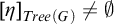 .
.
We show that
${Tree}(G)$
 is c.l.c. via
$k=1$
is c.l.c. via
$k=1$
 . Note that if
$\sigma \in {Tree}(G)$
. Note that if
$\sigma \in {Tree}(G)$
 maps
$x\in T_d$
maps
$x\in T_d$
 to
$y\in T_d$
to
$y\in T_d$
 , then every extension
$\eta \in {Tree}(G) $
, then every extension
$\eta \in {Tree}(G) $
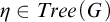 of
$\sigma $
of
$\sigma $
 maps elements in
$T_d$
maps elements in
$T_d$
 at distance n from x to elements in
$T_d$
at distance n from x to elements in
$T_d$
 at distance n from y, and conversely. This yields a computable bound H as required in Definition 2.4.
The following lemma shows that, given a group G as in Definition 3.3, the group operations are algorithmic when applied to its compact open subsets.
Lemma 3.5. Suppose G is computably t.d.l.c. via a closed subgroup of
$S_\infty $
 (identified with G). Write
$T = {Tree}(G) $
(identified with G). Write
$T = {Tree}(G) $
 , which by hypothesis is c.l.c. via some
$k \in {\mathbb {N}}^+$
, which by hypothesis is c.l.c. via some
$k \in {\mathbb {N}}^+$
 . Recall from Definitions 2.5 and 2.7 that
$\mathcal {K}_u$
. Recall from Definitions 2.5 and 2.7 that
$\mathcal {K}_u$
 denotes the open subset of
$[T]$
denotes the open subset of
$[T]$
 with code number u, where u is a strong index for a finite subset of
$T^{[\ge k]}$
with code number u, where u is a strong index for a finite subset of
$T^{[\ge k]}$
 ;
$ E_T\subseteq {\mathbb {N}}$
;
$ E_T\subseteq {\mathbb {N}}$
 denotes the computable set of minimal code numbers for compact open subsets of
$[T]$
denotes the computable set of minimal code numbers for compact open subsets of
$[T]$
 .
.
-
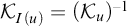
(i) There is a computable function $ I \colon E_T \to E_T$
such that
$\mathcal {K}_{I(u)} = (\mathcal {K}_u)^{-1}$
for each
$u \in E_T$
. -
(ii) There is a computable function $M \colon E_T \times E_T \to E_T$
such that
$ \mathcal {K}_{M(u,v)}= \mathcal {K}_u \mathcal {K}_v$
for each
$u,v \in E_T$
.





Proof. We will use Lemma 2.6 without special mention. For (i), let
$I(u) $
 be the least strong index for the set
$ \{ \sigma _1 \oplus \sigma _0 \colon \, \sigma _0\oplus \sigma _1 \in u\}$
be the least strong index for the set
$ \{ \sigma _1 \oplus \sigma _0 \colon \, \sigma _0\oplus \sigma _1 \in u\}$
 . For (ii), first note that since
${Tree}(G) $
. For (ii), first note that since
${Tree}(G) $
 is c.l.c. via k, we can computably replace each string
$\sigma $
is c.l.c. via k, we can computably replace each string
$\sigma $
 in u by its set of extensions on
${Tree}(G) $
in u by its set of extensions on
${Tree}(G) $
 of a given length
$N \ge |\sigma |$
of a given length
$N \ge |\sigma |$
 . So we may assume that all the strings in
$u\cup v$
. So we may assume that all the strings in
$u\cup v$
 have the same length. Hence it suffices to define
$M(u,v)$
have the same length. Hence it suffices to define
$M(u,v)$
 in case that
$u = \{\sigma \}$
in case that
$u = \{\sigma \}$
 and
$ v= \{ \tau \}$
and
$ v= \{ \tau \}$
 where
$|\sigma |= |\tau | =:n$
where
$|\sigma |= |\tau | =:n$
 .
.
For such
$\sigma , \tau $
 let
$m = 1 + \max (\sigma , \tau )$
let
$m = 1 + \max (\sigma , \tau )$
 ; that is,
$m-1$
; that is,
$m-1$
 is the maximum number occurring in any of the two strings. For strings
$\gamma , \delta \in {\mathbb {N}}^*$
is the maximum number occurring in any of the two strings. For strings
$\gamma , \delta \in {\mathbb {N}}^*$
 such that
$|\delta |\ge 1+\max (\gamma )$
such that
$|\delta |\ge 1+\max (\gamma )$
 , by
$\delta \cdot \gamma $
, by
$\delta \cdot \gamma $
 we denote the string
${\langle {\delta (\gamma (i))}\rangle }_{i < |\gamma |}$
we denote the string
${\langle {\delta (\gamma (i))}\rangle }_{i < |\gamma |}$
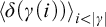 . We will verify that for each
$f \in G$
. We will verify that for each
$f \in G$
 ,
,

where
$\alpha = \alpha _0 \oplus \alpha _1$
 ,
$\beta = \beta _0 \oplus \beta _1$
,
$\beta = \beta _0 \oplus \beta _1$
 , and
$f = f_0 \oplus f_1$
, and
$f = f_0 \oplus f_1$
 as usual. Given this, we let
$M(u,v)$
as usual. Given this, we let
$M(u,v)$
 be the least strong index for the set of strings
$(\beta _0 \cdot \sigma _0\oplus \alpha _1 \cdot \tau _1)$
be the least strong index for the set of strings
$(\beta _0 \cdot \sigma _0\oplus \alpha _1 \cdot \tau _1)$
 as above, which we can compute from u and v by the hypothesis on T. This will complete the proof of (ii) of the claim.
If the left hand side of (2) holds, then
$f = h g$
 for some
$g,h\in G$
for some
$g,h\in G$
 such that
$\sigma \prec g$
such that
$\sigma \prec g$
 and
$\tau \prec h$
and
$\tau \prec h$
 . Then the right hand side holds via
$\beta = h \upharpoonright {2m}$
. Then the right hand side holds via
$\beta = h \upharpoonright {2m}$
 and
$\alpha = g \upharpoonright (2\max \beta +2) $
and
$\alpha = g \upharpoonright (2\max \beta +2) $
 .
.
Now suppose that the right hand side of (2) holds. Since
$\beta \in T$
 , there is
$h \in G$
, there is
$h \in G$
 such that
$h \succ \beta $
such that
$h \succ \beta $
 . Let
$g = h^{-1} f$
. Let
$g = h^{-1} f$
 . Then
$g\in G$
. Then
$g\in G$
 . Since
$h \succ \tau $
. Since
$h \succ \tau $
 , it suffices to show that
$g \succ \sigma $
, it suffices to show that
$g \succ \sigma $
 . Note that by definition
$f = f_0 \oplus f_1$
. Note that by definition
$f = f_0 \oplus f_1$
 where
$f_1= (f_0)^{-1}$
where
$f_1= (f_0)^{-1}$
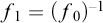 , and similarly
$g= g_0 \oplus g_1 $
, and similarly
$g= g_0 \oplus g_1 $
 and
$ h= h_0 \oplus h_1$
and
$ h= h_0 \oplus h_1$
 . We have
$g_0 = h_1 \circ f_0$
. We have
$g_0 = h_1 \circ f_0$
 and
$g_1 = f_1 \circ h_0$
and
$g_1 = f_1 \circ h_0$
 .
.
We check that
$g_0 \succ \sigma _0$
 as follows: for each
$i< n$
as follows: for each
$i< n$
 we have
$\beta _0(\sigma _0(i))= f_0(i)$
we have
$\beta _0(\sigma _0(i))= f_0(i)$
 by hypothesis. Hence
$h_0(\sigma _0(i))= f_0(i)$
by hypothesis. Hence
$h_0(\sigma _0(i))= f_0(i)$
 , so
$\sigma _0(i)= h_1(f_0(i))= g_0(i)$
, so
$\sigma _0(i)= h_1(f_0(i))= g_0(i)$
 .
.
Next, we check that
$g_1 \succ \sigma _1$
 : using
$ \alpha _1 \cdot \beta _1 \prec f_1$
: using
$ \alpha _1 \cdot \beta _1 \prec f_1$
 , for each
$i< n$
, for each
$i< n$
 we have

Since
$\beta \in T$
 ,
$\beta _0 \succ \tau _0$
,
$\beta _0 \succ \tau _0$
 , and
$|\beta _1|> \max (\tau _0)$
, and
$|\beta _1|> \max (\tau _0)$
 , we have
$\beta _1(\tau _0(i))=i$
, we have
$\beta _1(\tau _0(i))=i$
 . So the value of the rightmost term is
$\alpha _1(i)$
. So the value of the rightmost term is
$\alpha _1(i)$
 , which equals
$\sigma _1(i)$
, which equals
$\sigma _1(i)$
 .
.
4 Defining computably t.d.l.c. groups via meet groupoids.
This section provides detail on the second type (Type M) of computable presentations of t.d.l.c. groups described in Section 1.4.
4.1 The meet groupoid of a t.d.l.c. group.
Intuitively, the notion of a groupoid generalizes the notion of a group by allowing that the binary operation is partial. A groupoid is given by a domain
$\mathcal {W}$
 on which a unary operation
$(.)^{-1}$
on which a unary operation
$(.)^{-1}$
 and a partial binary operation, denoted by “
$\cdot $
and a partial binary operation, denoted by “
$\cdot $
 ”, are defined. These operations satisfy the following conditions:
-
(a) associativity in the sense that $(A \cdot B)\cdot C= A \cdot (B\cdot C)$
, with either both sides or no side defined (and so the parentheses can be omitted); -
(b) $A\cdot A^{-1}$
and
$A^{-1}\cdot A$
are always defined; -
(c) if $A\cdot B$
is defined then
$A\cdot B\cdot B^{-1}=A$
and
$A^{-1}\cdot A\cdot B =B$
.




It follows from (c) that a groupoid satisfies the left and right cancellation laws. One says that an element
$U\in \mathcal {W}$
 is idempotent if
$U\cdot U =U$
is idempotent if
$U\cdot U =U$
 . Clearly this implies that
$U= U \cdot U^{-1}= U^{-1} \cdot U$
. Clearly this implies that
$U= U \cdot U^{-1}= U^{-1} \cdot U$
 and so
$U= U^{-1}$
and so
$U= U^{-1}$
 by cancellation. Conversely, by (c) every element of the form
$A\cdot A^{-1}$
by cancellation. Conversely, by (c) every element of the form
$A\cdot A^{-1}$
 or
$A^{-1}\cdot A$
or
$A^{-1}\cdot A$
 is idempotent.
Definition 4.1. A meet groupoid is a groupoid
$(\mathcal {W}, \cdot , {(.)}^{-1})$
 that is also a meet semilattice
$(\mathcal {W}, \cap ,\emptyset )$
that is also a meet semilattice
$(\mathcal {W}, \cap ,\emptyset )$
 of which
$\emptyset $
of which
$\emptyset $
 is the least element. Writing
$A \subseteq B \Leftrightarrow A\cap B = A$
is the least element. Writing
$A \subseteq B \Leftrightarrow A\cap B = A$
 and letting the operation
$\cdot $
and letting the operation
$\cdot $
 have preference over
$\cap $
have preference over
$\cap $
 , it satisfies the conditions:
-
(d) $\emptyset ^{-1} = \emptyset = \emptyset \cdot \emptyset $
, and
$\emptyset \cdot A$
and
$A \cdot \emptyset $
are undefined for each
$A \neq \emptyset $
, -
(e) if $U,V$
are idempotents such that
$U,V \neq \emptyset $
, then
$U \cap V \neq \emptyset $
,



-
(f) $A \subseteq B \Leftrightarrow A^{-1} \subseteq B^{-1}$
, and -
(g) if $A_i\cdot B_i$
are defined (
$i= 0,1$
) and
$A_0 \cap A_1 \neq \emptyset \neq B_0 \cap B_1$
, then $$ \begin{align*} (A_0 \cap A_1)\cdot (B_0 \cap B_1) = A_0 \cdot B_0 \cap A_1 \cdot B_1. \end{align*} $$





Item (g) implies that the groupoid operations are monotonic: if
$A_i\cdot B_i$
 are defined (
$i= 0,1$
are defined (
$i= 0,1$
 ) and
$A_0 \subseteq A_1, B_0 \subseteq B_1 $
) and
$A_0 \subseteq A_1, B_0 \subseteq B_1 $
 , then
$A_0 \cdot B_0 \subseteq A_1 \cdot B_1$
, then
$A_0 \cdot B_0 \subseteq A_1 \cdot B_1$
 . Also, if U and V are idempotent, then so is
$U \cap V$
. Also, if U and V are idempotent, then so is
$U \cap V$
 (this can also be verified based on (a)–(f) alone).
Given meet groupoids
$\mathcal {W}_0, \mathcal {W}_1$
 , a bijection
$h \colon \mathcal {W}_0 \to \mathcal {W}_1$
, a bijection
$h \colon \mathcal {W}_0 \to \mathcal {W}_1$
 is an isomorphism if it preserves the three operations. Given a meet groupoid
$\mathcal {W}$
is an isomorphism if it preserves the three operations. Given a meet groupoid
$\mathcal {W}$
 , the letters
$A,B, C$
, the letters
$A,B, C$
 will range over elements of
$\mathcal {W}$
will range over elements of
$\mathcal {W}$
 , and the letters
$U,V,W$
, and the letters
$U,V,W$
 will range over idempotents.
We use set theoretic notation for the meet semilattice because the ordering for the motivating examples of meet groupoids is given by set inclusion.
Definition 4.2. Let G be a t.d.l.c. group. We define a meet groupoid
$\mathcal {W}(G)$
 . Its domain consists of the compact open cosets in G (i.e., cosets of compact open subgroups of G), as well as the empty set. We define
$A\cdot B$
. Its domain consists of the compact open cosets in G (i.e., cosets of compact open subgroups of G), as well as the empty set. We define
$A\cdot B$
 to be the usual product
$AB$
to be the usual product
$AB$
 in case that
$A= B= \emptyset $
in case that
$A= B= \emptyset $
 , or A is a left coset of a subgroup V and B is a right coset of V; otherwise
$A \cdot B$
, or A is a left coset of a subgroup V and B is a right coset of V; otherwise
$A \cdot B$
 is undefined.
Fact 4.3.
$\mathcal {W}(G)$
 is a meet groupoid with the groupoid operations of
$\cdot $
is a meet groupoid with the groupoid operations of
$\cdot $
 and inversion, and the usual intersection operation
$\cap $
and inversion, and the usual intersection operation
$\cap $
 .
.
Proof. We first note that
$\mathcal {W}(G)$
 is closed under the operation
$\cap $
is closed under the operation
$\cap $
 : if C and D are right cosets of subgroups U and V, respectively, and if
$g \in C \cap D$
: if C and D are right cosets of subgroups U and V, respectively, and if
$g \in C \cap D$
 , then
$C \cap D= (U \cap V)g$
, then
$C \cap D= (U \cap V)g$
 .
.
Item (a) is clear from the definition. For (b), if
$A = gU$
 then
$A^{-1}= Ug^{-1}$
then
$A^{-1}= Ug^{-1}$
 , so
$A \cdot A^{-1}$
, so
$A \cdot A^{-1}$
 is defined. The case of
$A^{-1} \cdot A$
is defined. The case of
$A^{-1} \cdot A$
 is similar. For (c), let A be a left coset of U and B a right coset of U. Then
$B \cdot B^{-1}= U$
is similar. For (c), let A be a left coset of U and B a right coset of U. Then
$B \cdot B^{-1}= U$
 , so
$A\cdot U =A$
, so
$A\cdot U =A$
 . The other case is symmetric. Item (d) is again clear from the definition, (e) follows because idempotents are subgroups by the discussion before Definition 4.1, and (f) is immediate.
To verify item (g), let
$A_i$
 be a right coset of a subgroup
$U_i$
be a right coset of a subgroup
$U_i$
 and a left coset of subgroup
$V_i$
and a left coset of subgroup
$V_i$
 , so that
$B_i$
, so that
$B_i$
 is a right coset of
$V_i$
is a right coset of
$V_i$
 by hypothesis. Then
$A_0 \cap A_1 $
by hypothesis. Then
$A_0 \cap A_1 $
 is a right coset of
$U_0 \cap U_1$
is a right coset of
$U_0 \cap U_1$
 , and
$B_0 \cap B_1$
, and
$B_0 \cap B_1$
 is a right coset of
$V_0 \cap V_1$
is a right coset of
$V_0 \cap V_1$
 , so the left hand side is defined and is a right coset of
$U_0 \cap U_1$
, so the left hand side is defined and is a right coset of
$U_0 \cap U_1$
 . The left hand side is clearly contained in the right hand side, which is a right coset of
$U_0 \cap U_1$
. The left hand side is clearly contained in the right hand side, which is a right coset of
$U_0 \cap U_1$
 as well. So the two sides must be equal.
We note that
$\mathcal {W}(G)$
 satisfies the axioms of inductive groupoids posited in Lawson [Reference Lawson25, p. 109]. (See [Reference Nies38, Section 4] for more on an axiomatic approach to meet groupoids.)
We will apply the usual group theoretic terminology to elements of an abstract meet groupoid
$\mathcal {W}$
 . If U is an idempotent of
$\mathcal {W}$
. If U is an idempotent of
$\mathcal {W}$
 we call U a subgroup, if
$AU = A$
we call U a subgroup, if
$AU = A$
 we call A a left coset of U, and if
$UB= B$
we call A a left coset of U, and if
$UB= B$
 we call B a right coset of U. Based on the axioms, one can verify that if
$U \subseteq V$
we call B a right coset of U. Based on the axioms, one can verify that if
$U \subseteq V$
 for subgroups
$U,V$
for subgroups
$U,V$
 , then the map
$A \mapsto A^{-1}$
, then the map
$A \mapsto A^{-1}$
 induces a bijection between the left cosets and the right cosets of U contained in V.
Remark 4.4. It is well-known [Reference Higgins18] that one can view groupoids as small categories in which every morphism has an inverse. The elements of the groupoid are the morphisms of the category. The idempotent morphisms correspond to the objects of the category. One has
$A\colon U \to V$
 where
$U= A \cdot A^{-1}$
where
$U= A \cdot A^{-1}$
 and
$V= A^{-1} \cdot A$
and
$V= A^{-1} \cdot A$
 . Thus, in
$\mathcal {W}(G)$
. Thus, in
$\mathcal {W}(G)$
 ,
$A\colon U \to V$
,
$A\colon U \to V$
 means that A is a right coset of U and a left coset of V.
4.2 Second definition of computably t.d.l.c. groups.
Definition 4.5 (Haar computable meet groupoids).
A meet groupoid
$\mathcal {W}$
 is called Haar computable if
-
(a) its domain is a computable subset D of ${\mathbb {N}}$
; -
(b) the groupoid and meet operations are computable in the sense of Definition 1.3; in particular, the relation $\{ \langle x,y \rangle \colon \, x,y \in D \, \land \, x\cdot y \text { is defined}\}$
is computable; -
(c) the partial function with domain contained in $D \times D$
sending a pair of subgroups
$U, V\in \mathcal {W} $
to
$|U:U\cap V|$
is computable.


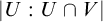
Here
$|U \colon U \cap V|$
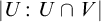 is defined abstractly as the number of left, or equivalently right, cosets of the nonzero idempotent
$U \cap V$
is defined abstractly as the number of left, or equivalently right, cosets of the nonzero idempotent
$U \cap V$
 contained in U; we implicitly require that this number is always finite. Note that by (b), the partial order induced by the meet semilattice structure of
$\mathcal {W}$
contained in U; we implicitly require that this number is always finite. Note that by (b), the partial order induced by the meet semilattice structure of
$\mathcal {W}$
 is computable. Also, (b) implies that being a subgroup is decidable when viewed as a property of elements of the domain D; this is used in (c). Condition (c) corresponds to the computable bound
$H(\sigma , i)$
is computable. Also, (b) implies that being a subgroup is decidable when viewed as a property of elements of the domain D; this is used in (c). Condition (c) corresponds to the computable bound
$H(\sigma , i)$
 required in (3) of Definition 2.4. For ease of reading we will say that
$n \in D$
required in (3) of Definition 2.4. For ease of reading we will say that
$n \in D$
 denotes a coset A, rather than saying that n “is” a coset.
Definition 4.6 (Computably t.d.l.c. groups via meet groupoids).
Let G be a t.d.l.c. group. We say that G is computably t.d.l.c. via a meet groupoid if
$\mathcal {W}(G)$
 has a Haar computable copy
$\mathcal {W}$
has a Haar computable copy
$\mathcal {W}$
 . In this context, we call
$\mathcal {W}$
. In this context, we call
$\mathcal {W}$
 a computable presentation of G (in the sense of meet groupoids).
Remark 4.7. In this setting, Condition (c) of Definition 4.5 is equivalent to saying that every Haar measure
$\mu $
 on G that assigns a rational number to some compact open subgroup (and hence is rational-valued) is computable on
$\mathcal {W}$
on G that assigns a rational number to some compact open subgroup (and hence is rational-valued) is computable on
$\mathcal {W}$
 , in the sense that the function assigning to a compact open coset
$ A$
, in the sense that the function assigning to a compact open coset
$ A$
 the rational
$\mu (A)$
the rational
$\mu (A)$
 is computable. Consider left Haar measures, say. First suppose that (c) holds. Given A, compute the subgroup V such that
$A= A\cdot V$
is computable. Consider left Haar measures, say. First suppose that (c) holds. Given A, compute the subgroup V such that
$A= A\cdot V$
 , i.e., A is a left coset of V. Compute
$W = U \cap V$
, i.e., A is a left coset of V. Compute
$W = U \cap V$
 . We have
$\mu (A) = \mu (V)= \mu (U) \cdot |V:W|/|U:W|$
. We have
$\mu (A) = \mu (V)= \mu (U) \cdot |V:W|/|U:W|$
 .
.
Conversely, if the Haar measure is computable on
$\mathcal {W}$
 , then (c) holds because
$|U\colon V|= \mu (U)/\mu (V)$
, then (c) holds because
$|U\colon V|= \mu (U)/\mu (V)$
 .
.
For discrete groups, the condition (c) can be dropped, as the proof of the following shows.
Example 4.8. A countable discrete group G is computably t.d.l.c. via a meet groupoid
$\Leftrightarrow G$
 has a computable copy in the usual sense of Definition 1.4.
Proof. For the implication
$\Leftarrow $
 , we may assume that G itself is computable; in particular, we may assume that its domain is a computable subset of
${\mathbb {N}}$
, we may assume that G itself is computable; in particular, we may assume that its domain is a computable subset of
${\mathbb {N}}$
 . Each compact coset in G is finite, and hence can be represented by a strong index for a finite set of natural numbers. Since the group operations are computable on the domain, this implies that the meet groupoid of G has a computable copy. It is then trivially Haar computable.
For the implication
$\Rightarrow $
 , let
$\mathcal {W}$
, let
$\mathcal {W}$
 be a Haar computable copy of
$\mathcal {W}(G)$
be a Haar computable copy of
$\mathcal {W}(G)$
 . Since G is discrete,
$\mathcal {W}$
. Since G is discrete,
$\mathcal {W}$
 contains a least subgroup U. The set of left cosets of U is computable, and forms a group with the groupoid and inverse operations. This yields the required computable copy of G.
By
$\mathbb {Q}_p$
 we denote the additive group of the p-adics. By the usual definition of semidirect products [Reference Robinson48, p. 27],
${\mathbb {Z}} \ltimes {\mathbb {Q}}_p$
we denote the additive group of the p-adics. By the usual definition of semidirect products [Reference Robinson48, p. 27],
${\mathbb {Z}} \ltimes {\mathbb {Q}}_p$
 is the group defined on the Cartesian product
${\mathbb {Z}} \times {\mathbb {Q}}_p$
is the group defined on the Cartesian product
${\mathbb {Z}} \times {\mathbb {Q}}_p$
 via the binary operation
$\langle z_1, \alpha _1 \rangle \cdot \langle z_2, \alpha _2\rangle = \langle z_1 + z_2, p^{z_2} \alpha _1 + \alpha _2\rangle $
via the binary operation
$\langle z_1, \alpha _1 \rangle \cdot \langle z_2, \alpha _2\rangle = \langle z_1 + z_2, p^{z_2} \alpha _1 + \alpha _2\rangle $
 . This turns
${\mathbb {Z}} \ltimes {\mathbb {Q}}_p$
. This turns
${\mathbb {Z}} \ltimes {\mathbb {Q}}_p$
 into a topological group with the product topology.
Proposition 4.9. For any prime p, the additive group
${\mathbb {Q}}_p$
 and the group
${\mathbb {Z}} \ltimes {\mathbb {Q}}_p$
and the group
${\mathbb {Z}} \ltimes {\mathbb {Q}}_p$
 are computably t.d.l.c. via a meet groupoid.
Proof. We begin with the additive group
${\mathbb {Q}}_p$
 . Note that its open proper subgroups are of the form
$U_r:= p^{r}{\mathbb {Z}}_p$
. Note that its open proper subgroups are of the form
$U_r:= p^{r}{\mathbb {Z}}_p$
 for some
$r\in {\mathbb {Z}}$
for some
$r\in {\mathbb {Z}}$
 . Let
$C_{p^\infty }$
. Let
$C_{p^\infty }$
 denote the Prüfer group
${\mathbb {Z}}[1/p]/{\mathbb {Z}}$
denote the Prüfer group
${\mathbb {Z}}[1/p]/{\mathbb {Z}}$
 , where
${\mathbb {Z}}[1/p]= \{ z p^{-k} \colon \, z \in {\mathbb {Z}} \, \land \, k \in {\mathbb {N}}\}$
, where
${\mathbb {Z}}[1/p]= \{ z p^{-k} \colon \, z \in {\mathbb {Z}} \, \land \, k \in {\mathbb {N}}\}$
 . For each r there is a canonical epimorphism
$\pi _r\colon {\mathbb {Q}}_p \to C_{p^\infty }$
. For each r there is a canonical epimorphism
$\pi _r\colon {\mathbb {Q}}_p \to C_{p^\infty }$
 with kernel
$U_r$
with kernel
$U_r$
 : if
$\alpha = \sum _{i=-n}^\infty s_ip^i$
: if
$\alpha = \sum _{i=-n}^\infty s_ip^i$
 where
$0 \le s_i < p$
where
$0 \le s_i < p$
 ,
$n\in {\mathbb {N}}$
,
$n\in {\mathbb {N}}$
 , we have

here an empty sum is interpreted as
$0$
 . (Informally,
$\pi _r(\alpha )$
. (Informally,
$\pi _r(\alpha )$
 is obtained by taking the “tail” of
$\alpha $
is obtained by taking the “tail” of
$\alpha $
 from the position
$r-1$
from the position
$r-1$
 onwards to the last position, and shifting it in order to represent an element of
$C_{p^\infty }$
onwards to the last position, and shifting it in order to represent an element of
$C_{p^\infty }$
 .) So each compact open coset in
${\mathbb {Q}}_p$
.) So each compact open coset in
${\mathbb {Q}}_p$
 can be uniquely written in the form
$D_{r,a}= \pi _r^{-1}(a)$
can be uniquely written in the form
$D_{r,a}= \pi _r^{-1}(a)$
 for some
$r \in {\mathbb {Z}}$
for some
$r \in {\mathbb {Z}}$
 and
$a \in C_{p^\infty }$
and
$a \in C_{p^\infty }$
 . The domain
$S\subseteq {\mathbb {N}}$
. The domain
$S\subseteq {\mathbb {N}}$
 of the Haar computable copy
$\mathcal {W}$
of the Haar computable copy
$\mathcal {W}$
 of
$\mathcal {W}({\mathbb {Q}}_p)$
of
$\mathcal {W}({\mathbb {Q}}_p)$
 consists of the natural numbers encoding such pairs
$\langle r,a\rangle $
consists of the natural numbers encoding such pairs
$\langle r,a\rangle $
 according to some fixed encoding. They will be identified with the cosets they denote.
The groupoid operations are computable because we have
$D_{r,a}^{-1}= D_{r,-a}$
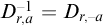 , and
$D_{r,a} \cdot D_{s,b}= D_{r, a+b}$
, and
$D_{r,a} \cdot D_{s,b}= D_{r, a+b}$
 if
$r=s$
if
$r=s$
 , and undefined otherwise. It is easy to check that
$D_{r,a} \subseteq D_{s,b}$
, and undefined otherwise. It is easy to check that
$D_{r,a} \subseteq D_{s,b}$
 iff
$r \ge s$
iff
$r \ge s$
 and
$p^{r-s}a=b$
and
$p^{r-s}a=b$
 . So the inclusion relation is decidable. We have
$D_{r,a} \cap D_{s,b}= \emptyset $
. So the inclusion relation is decidable. We have
$D_{r,a} \cap D_{s,b}= \emptyset $
 unless one of the sets is contained in the other, so the meet operation is computable. Finally, for
$r\le s$
unless one of the sets is contained in the other, so the meet operation is computable. Finally, for
$r\le s$
 , we have
$|U_r: U_s|= p^{s-r}$
, we have
$|U_r: U_s|= p^{s-r}$
 which is computable.
Next, let
$G = {\mathbb {Z}} \ltimes {\mathbb {Q}}_p$
 ; we build a Haar computable copy
$\mathcal {V}$
; we build a Haar computable copy
$\mathcal {V}$
 of
$ \mathcal {W} (G)$
of
$ \mathcal {W} (G)$
 . We will extend the listing
$(D_{r,a})_{r \in {\mathbb {Z}}, a \in C_{p^\infty }}$
. We will extend the listing
$(D_{r,a})_{r \in {\mathbb {Z}}, a \in C_{p^\infty }}$
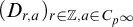 of compact open cosets in
${\mathbb {Q}}_p$
of compact open cosets in
${\mathbb {Q}}_p$
 given above. For each compact open subgroup of G, the projection onto
${\mathbb {Z}}$
given above. For each compact open subgroup of G, the projection onto
${\mathbb {Z}}$
 is a compact open subgroup of
${\mathbb {Z}}$
is a compact open subgroup of
${\mathbb {Z}}$
 , and hence trivial. So the only compact open subgroups of G are of the form
$U_r$
, and hence trivial. So the only compact open subgroups of G are of the form
$U_r$
 . Let
$g\in G$
. Let
$g\in G$
 be the generator of
${\mathbb {Z}}$
be the generator of
${\mathbb {Z}}$
 such that
$g^{-1} \alpha g = p \alpha $
such that
$g^{-1} \alpha g = p \alpha $
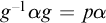 for each
$\alpha \in {\mathbb {Q}}_p$
for each
$\alpha \in {\mathbb {Q}}_p$
 (where
${\mathbb {Z}}$
(where
${\mathbb {Z}}$
 and
${\mathbb {Q}}_p$
and
${\mathbb {Q}}_p$
 are thought of as canonically embedded into G). Each compact open coset of G has a unique form
$g^z D_{r,a}$
are thought of as canonically embedded into G). Each compact open coset of G has a unique form
$g^z D_{r,a}$
 for some
$z \in {\mathbb {Z}}$
for some
$z \in {\mathbb {Z}}$
 . Formally speaking, the domain of the computable copy of
$\mathcal {W}(G)$
. Formally speaking, the domain of the computable copy of
$\mathcal {W}(G)$
 consists of natural numbers encoding the triples
$\langle z, r, a\rangle $
consists of natural numbers encoding the triples
$\langle z, r, a\rangle $
 corresponding to such cosets according to some fixed encoding; as before they will be identified with the cosets they denote.
To show that the groupoid and meet operations are computable, note that we have
$gD_{r, a } = D_{r-1, a} g $
 for each
$r \in {\mathbb {Z}}, a \in C_{p^\infty }$
for each
$r \in {\mathbb {Z}}, a \in C_{p^\infty }$
 , and hence
$ g^z D_{r, a } = D_{r-z, a} g^z $
, and hence
$ g^z D_{r, a } = D_{r-z, a} g^z $
 for each
$z \in {\mathbb {Z}}$
for each
$z \in {\mathbb {Z}}$
 . Given two cosets
$g^v D_{r,a} $
. Given two cosets
$g^v D_{r,a} $
 and
$ g^w D_{s,b}= D_{s-w, b}g^w$
and
$ g^w D_{s,b}= D_{s-w, b}g^w$
 , their composition is defined iff
$r=s-w$
, their composition is defined iff
$r=s-w$
 , in which case the result is
$g^{v+w} D_{s,a+b}$
, in which case the result is
$g^{v+w} D_{s,a+b}$
 . The inverse of
$g^z D_{r,a}$
. The inverse of
$g^z D_{r,a}$
 is
$D_{r, -a}g^{-z} = g^{-z}D_{r-z, -a}$
is
$D_{r, -a}g^{-z} = g^{-z}D_{r-z, -a}$
 .
.
To decide the inclusion relation, note that we have
$g^z D_{r,a} \subseteq g^w D_{s,b}$
 iff
$z=w$
iff
$z=w$
 and
$D_{r,a} \subseteq D_{s,b}$
and
$D_{r,a} \subseteq D_{s,b}$
 , and otherwise, they are disjoint. Using this, one can show that the meet operation is computable (by an argument that works in any computable meet groupoid
$\mathcal {V}$
, and otherwise, they are disjoint. Using this, one can show that the meet operation is computable (by an argument that works in any computable meet groupoid
$\mathcal {V}$
 ): recalling the notation in Remark 4.4, if
$A_0, A_1 \in \mathcal {V}$
): recalling the notation in Remark 4.4, if
$A_0, A_1 \in \mathcal {V}$
 ,
$A_i \colon U_i \to V_i$
,
$A_i \colon U_i \to V_i$
 , and
$A_0,A_1$
, and
$A_0,A_1$
 are not disjoint, then
$A_0 \cap A_1$
are not disjoint, then
$A_0 \cap A_1$
 is the unique
$C \in \mathcal {V}$
is the unique
$C \in \mathcal {V}$
 such that
$C \colon U_0 \cap U_1 \to V_0 \cap V_1$
such that
$C \colon U_0 \cap U_1 \to V_0 \cap V_1$
 and
$C\subseteq A_0, A_1$
and
$C\subseteq A_0, A_1$
 . Since
$\mathcal {W}$
. Since
$\mathcal {W}$
 satisfies Condition (c) in Definition 4.5, and
$\mathcal {V}$
satisfies Condition (c) in Definition 4.5, and
$\mathcal {V}$
 has no subgroups beyond the ones present in
$ \mathcal {W}$
has no subgroups beyond the ones present in
$ \mathcal {W}$
 , we conclude that
$\mathcal {V}$
, we conclude that
$\mathcal {V}$
 is Haar computable.
5 Uniform equivalence of two definitions of computably t.d.l.c.
We show that Definitions 3.3 and 4.6 of computably t.d.l.c. groups are equivalent in a computationally uniform way. This provides a first evidence for the robustness of this class of t.d.l.c. groups.
Theorem 5.1. A group G is computably t.d.l.c. via a closed subgroup of
$S_\infty \Leftrightarrow $
 G is computably t.d.l.c. via a meet groupoid.
Moreover, from a presentation of G of one type, one can effectively obtain a presentation of G of the other type.
Proof. “
$\Rightarrow $
 ”: Suppose that G is computably t.d.l.c. as a closed subgroup of
$S_\infty $
”: Suppose that G is computably t.d.l.c. as a closed subgroup of
$S_\infty $
 . To save on notation, we may assume that G itself is a closed subgroup of
$S_\infty $
. To save on notation, we may assume that G itself is a closed subgroup of
$S_\infty $
 showing this. We will obtain a Haar computable copy of its meet groupoid
$\mathcal {W}(G)$
showing this. We will obtain a Haar computable copy of its meet groupoid
$\mathcal {W}(G)$
 .
.
Recall from Definition 2.7 that
$E=E_{{Tree}(G) }\subseteq {\mathbb {N}}$
 is the decidable set of minimal code numbers for compact open subsets of G. For
$u \in E$
is the decidable set of minimal code numbers for compact open subsets of G. For
$u \in E$
 we can decide whether
$\mathcal {K}_u$
we can decide whether
$\mathcal {K}_u$
 is a subgroup: this is the case precisely when
$\mathcal {K}_{M(u,u)}= \mathcal {K}_u$
is a subgroup: this is the case precisely when
$\mathcal {K}_{M(u,u)}= \mathcal {K}_u$
 and
$\mathcal {K}_{I(u)} = \mathcal {K}_u$
and
$\mathcal {K}_{I(u)} = \mathcal {K}_u$
 , where the computable functions
$I,M$
, where the computable functions
$I,M$
 were defined in Lemma 3.5. We can also decide whether
$B=\mathcal {K}_v$
were defined in Lemma 3.5. We can also decide whether
$B=\mathcal {K}_v$
 is a coset: this is the case precisely when
$B B^{-1}$
is a coset: this is the case precisely when
$B B^{-1}$
 is a subgroup U (in which case B is its right coset). Equivalently,
$\mathcal {K}_{M(v,I(v))}$
is a subgroup U (in which case B is its right coset). Equivalently,
$\mathcal {K}_{M(v,I(v))}$
 is a subgroup, which is a decidable condition.
The domain D of the computable copy of
$\mathcal {W}(G)$
 is the subset of
$ E$
is the subset of
$ E$
 consisting of the code numbers for cosets. For cosets
$A= \mathcal {K}_u, B= \mathcal {K}_v \in \mathcal {W}(G)$
consisting of the code numbers for cosets. For cosets
$A= \mathcal {K}_u, B= \mathcal {K}_v \in \mathcal {W}(G)$
 recall that
$A \cdot B$
recall that
$A \cdot B$
 is defined iff A is a left coset of a subgroup V such that B is a right coset of V. Equivalently,
$\mathcal {K}_{M(I(u), u)}= \mathcal {K}_{M(v,I(v))}$
is defined iff A is a left coset of a subgroup V such that B is a right coset of V. Equivalently,
$\mathcal {K}_{M(I(u), u)}= \mathcal {K}_{M(v,I(v))}$
 , which is a decidable condition. So the groupoid operations and meet operation are computable.
It remains to show that,
$u,v\in D$
 coding subgroups
$U,V$
coding subgroups
$U,V$
 , one can compute
$|U : U \cap V|$
, one can compute
$|U : U \cap V|$
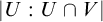 . To do so, one enumerates (code numbers in D of) left cosets of
$U \cap V$
. To do so, one enumerates (code numbers in D of) left cosets of
$U \cap V$
 contained in U, until their union equals U. (There is an algorithm to decide the latter condition by Lemma 2.6(i).) Then one outputs the number of cosets found.
“
$\Leftarrow $
 ”: The basic idea is that the left translation action of G on the given Haar computable presentation
$\mathcal {W}$
”: The basic idea is that the left translation action of G on the given Haar computable presentation
$\mathcal {W}$
 of its meet groupoid, namely
$\langle g, A \rangle \mapsto gA$
of its meet groupoid, namely
$\langle g, A \rangle \mapsto gA$
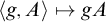 for
$g \in G, A \in \mathcal {W}$
for
$g \in G, A \in \mathcal {W}$
 , yields a computable presentation of G via a closed subgroup of
$S_\infty $
, yields a computable presentation of G via a closed subgroup of
$S_\infty $
 . The main work is to show that the group
$\widetilde G$
. The main work is to show that the group
$\widetilde G$
 of permutations of
$\mathcal {W}$
of permutations of
$\mathcal {W}$
 so obtained can be described by a c.l.c. tree (Definition 2.4) whose paths can be viewed as permutations.
To carry this out, we introduce an operator
$\mathcal {G}_{\text {comp}} $
 from meet groupoids to permutation groups that will be needed frequently later on. In case that
$\mathcal {W}$
from meet groupoids to permutation groups that will be needed frequently later on. In case that
$\mathcal {W}$
 is a copy of the meet groupoid of G, the operator produces the permutation group given by this left action of G. However, the operator can be defined based on the meet groupoid alone, and thus can be seen as a dual of the operator
$G \to \mathcal {W}(G)$
is a copy of the meet groupoid of G, the operator produces the permutation group given by this left action of G. However, the operator can be defined based on the meet groupoid alone, and thus can be seen as a dual of the operator
$G \to \mathcal {W}(G)$
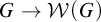 obtained in the first part of the proof.
We emphasise that the elements of
$S_\infty $
 are not actually permutations, but paths p on
$ {Tree}(S_\infty ) $
are not actually permutations, but paths p on
$ {Tree}(S_\infty ) $
 encoding pairs consisting of a permutation and its inverse. Nonetheless, if
$A \in \mathcal {W}$
encoding pairs consisting of a permutation and its inverse. Nonetheless, if
$A \in \mathcal {W}$
 is denoted by x, below we often suggestively write
$p(A)$
is denoted by x, below we often suggestively write
$p(A)$
 for the element of
$\mathcal {W}$
for the element of
$\mathcal {W}$
 denoted by
$p(2x)$
denoted by
$p(2x)$
 .
.
Definition 5.2. Given a meet groupoid
$\mathcal {W}$
 with domain
$D\subseteq {\mathbb {N}}$
with domain
$D\subseteq {\mathbb {N}}$
 , let
$\widetilde G= \mathcal {G}_{\text {comp}} (\mathcal {W})$
, let
$\widetilde G= \mathcal {G}_{\text {comp}} (\mathcal {W})$
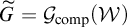 be the closed subgroup of
$ S_\infty $
be the closed subgroup of
$ S_\infty $
 consisting of elements p such that
$p(2x), p(2x+1) \in D$
consisting of elements p such that
$p(2x), p(2x+1) \in D$
 for each
$x \in D$
for each
$x \in D$
 ,
$p(2x )= p(2x+1)= x $
,
$p(2x )= p(2x+1)= x $
 for each
$x \not \in D$
for each
$x \not \in D$
 , and
, and
-
(a) p preserves the meet operation of $\mathcal {W;}$
-
(b) $p(A) \cdot B = p(A\cdot B) $
whenever
$A \cdot B$
is defined.



The formal conditions expressing (a) and (b) state that:
-
– for all $x,y \in D$
, we have
$p(2 (x \cap y))= p(2x) \cap p(2y)$
; -
– if $x \cdot y$
is defined then so is
$p(2x) \cdot y$
, and
$p(2x) \cdot y= p(2(x\cdot y))$
.





Note that such p can be identified with the automorphisms of the structure obtained from
$\mathcal {W}$
 which, instead of composition, for each B has a partial unary operation
$A \mapsto A \cdot B$
which, instead of composition, for each B has a partial unary operation
$A \mapsto A \cdot B$
 .
.
Suppose now that
$\mathcal {W}$
 is as in Definition 4.6. Then there is an isomorphism of meet groupoids
$ \mathcal {W} \to \mathcal {W}(G)$
is as in Definition 4.6. Then there is an isomorphism of meet groupoids
$ \mathcal {W} \to \mathcal {W}(G)$
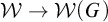 , which below we will use to identify
$\mathcal {W}$
, which below we will use to identify
$\mathcal {W}$
 and
$\mathcal {W}(G)$
and
$\mathcal {W}(G)$
 . We can make the assumptions that
$0\in D$
. We can make the assumptions that
$0\in D$
 , and that
$0$
, and that
$0$
 denotes a subgroup U in
$\mathcal {W}$
denotes a subgroup U in
$\mathcal {W}$
 , without affecting the uniformity statement of the theorem: otherwise we can search
$\mathcal {W}$
, without affecting the uniformity statement of the theorem: otherwise we can search
$\mathcal {W}$
 for the least n such that n is a subgroup, and then work with a new copy of
$\mathcal {W}(G)$
for the least n such that n is a subgroup, and then work with a new copy of
$\mathcal {W}(G)$
 where the roles of
$0$
where the roles of
$0$
 and n are swapped.
We note that for each subgroup
$U\in \mathcal {W}(G)$
 , the set
$B=p(U)$
, the set
$B=p(U)$
 is a left coset of U since
$B\cdot U = p(U)\cdot U= p(U\cdot U)= B$
is a left coset of U since
$B\cdot U = p(U)\cdot U= p(U\cdot U)= B$
 . Define a group homomorphism
$\Phi \colon G \to \widetilde G$
. Define a group homomorphism
$\Phi \colon G \to \widetilde G$
 by letting
$\Phi (g)$
by letting
$\Phi (g)$
 be the element of
$S_\infty $
be the element of
$S_\infty $
 corresponding to the left translation by g, i.e.,
$A \mapsto gA$
corresponding to the left translation by g, i.e.,
$A \mapsto gA$
 where
$A \in \mathcal {W}(G)$
where
$A \in \mathcal {W}(G)$
 . (See the comment after Definition 5.2.) Note that
$\Phi $
. (See the comment after Definition 5.2.) Note that
$\Phi $
 is injective because the compact open subgroups form a neighbourhood basis of
$1$
is injective because the compact open subgroups form a neighbourhood basis of
$1$
 : if
$g \neq 1$
: if
$g \neq 1$
 then
$g \not \in U$
then
$g \not \in U$
 for some compact open subgroup U, so that
$\Phi (g)(U) \neq U$
for some compact open subgroup U, so that
$\Phi (g)(U) \neq U$
 .
.
Claim 5.3.
$\Phi \colon G \to \widetilde G$
 is an isomorphism of topological groups.
To show that
$\Phi $
 is onto, let
$p \in \widetilde G$
is onto, let
$p \in \widetilde G$
 . Clearly the subgroups form a filter in
$\mathcal {W}(G)$
. Clearly the subgroups form a filter in
$\mathcal {W}(G)$
 . Using (a) this implies that
$\{p(U)\colon U \in \mathcal {W}(G) \text { is a subgroup}\}$
. Using (a) this implies that
$\{p(U)\colon U \in \mathcal {W}(G) \text { is a subgroup}\}$
 is also a filter on
$\mathcal {W}(G)$
is also a filter on
$\mathcal {W}(G)$
 . Since this filter contains a compact set, there is an element g in its intersection. Then
$\Phi (g)= p$
. Since this filter contains a compact set, there is an element g in its intersection. Then
$\Phi (g)= p$
 : since the set
$B=p(U)$
: since the set
$B=p(U)$
 is a left coset of U, it equals
$gU$
is a left coset of U, it equals
$gU$
 . So, if A is a right coset of U, then
$p(A)= p(U\cdot A)= B\cdot A = gA$
. So, if A is a right coset of U, then
$p(A)= p(U\cdot A)= B\cdot A = gA$
 .
.
To show that
$\Phi $
 is continuous at
$1$
is continuous at
$1$
 (and hence continuous), note that a basis of neighbourhoods of the identity in
$\widetilde G$
(and hence continuous), note that a basis of neighbourhoods of the identity in
$\widetilde G$
 is given by the open sets

where
$A_1, \ldots , A_n \in \mathcal {W}(G)$
 . Given such a set, suppose
$A_i$
. Given such a set, suppose
$A_i$
 is a right coset of
$U_i$
is a right coset of
$U_i$
 , and let
$U = \bigcap U_i$
, and let
$U = \bigcap U_i$
 . If
$g \in U$
. If
$g \in U$
 then
$gA_i = A_i$
then
$gA_i = A_i$
 for each i. By the open mapping theorem for Hausdorff groups Remark 1.2
$\Phi $
for each i. By the open mapping theorem for Hausdorff groups Remark 1.2
$\Phi $
 is open. This verifies the claim.
To complete the proof of the implication “
$\Leftarrow $
 ” of the theorem, we now show that
${Tree}(\widetilde G) $
” of the theorem, we now show that
${Tree}(\widetilde G) $
 is c.l.c. as in Definition 2.4, so that
$\widetilde G$
is c.l.c. as in Definition 2.4, so that
$\widetilde G$
 is a computable presentation of G via a closed subgroup of
$S_\infty $
is a computable presentation of G via a closed subgroup of
$S_\infty $
 as required. The following claim will be used to show that
${Tree}(\widetilde G) $
as required. The following claim will be used to show that
${Tree}(\widetilde G) $
 is computable, using the assumption that
$\mathcal {W}$
is computable, using the assumption that
$\mathcal {W}$
 is a computable meet groupoid. As usual by
$A,B$
is a computable meet groupoid. As usual by
$A,B$
 we denote compact open cosets of G, identified here with elements of
$D \subseteq {\mathbb {N}}$
we denote compact open cosets of G, identified here with elements of
$D \subseteq {\mathbb {N}}$
 , the domain of
$\mathcal {W}$
, the domain of
$\mathcal {W}$
 .
.
Claim 5.4. A finite injection
$\alpha $
 on
${\mathbb {N}}$
on
${\mathbb {N}}$
 can be extended to some
$p \in \widetilde G \Leftrightarrow $
can be extended to some
$p \in \widetilde G \Leftrightarrow $

$\alpha (x)= x$
 for each
$x \not \in D$
for each
$x \not \in D$
 , and
, and
$B\cdot A^{-1}$
 is defined whenever
$\alpha (A)= B$
is defined whenever
$\alpha (A)= B$
 , and
$\bigcap \{ B \cdot A^{-1} \colon \, \alpha (A) = B\} $
, and
$\bigcap \{ B \cdot A^{-1} \colon \, \alpha (A) = B\} $
 is non-empty.
“
$\Leftarrow $
 ”: Let g be an element of the intersection. Then
$gA = B\cdot A^{-1} \cdot A = B=\alpha (A)$
”: Let g be an element of the intersection. Then
$gA = B\cdot A^{-1} \cdot A = B=\alpha (A)$
 for each
$A \in \mathrm {dom} (\alpha )$
for each
$A \in \mathrm {dom} (\alpha )$
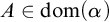 .
.
“
$\Rightarrow $
 ”: Suppose
$p\in \widetilde G $
”: Suppose
$p\in \widetilde G $
 extends
$\alpha $
extends
$\alpha $
 . By Claim 5.3, there is
$g\in G$
. By Claim 5.3, there is
$g\in G$
 such that
$p = \Phi (g)$
such that
$p = \Phi (g)$
 . Then
$gA = p(A) = B$
. Then
$gA = p(A) = B$
 for each
$A,B$
for each
$A,B$
 such that
$\alpha (A)= B$
such that
$\alpha (A)= B$
 . Such
$A,B$
. Such
$A,B$
 are right cosets of the same subgroup. Hence
$B\cdot A^{-1}$
are right cosets of the same subgroup. Hence
$B\cdot A^{-1}$
 is defined, and clearly g is in the intersection. This establishes the claim.
Recall from (1) in Section 3.1 that a string
$ \sigma \oplus \tau \in {Tree}(S_\infty ) $
 gives rise to a finite injection
$\alpha _{ \sigma \oplus \tau }$
gives rise to a finite injection
$\alpha _{ \sigma \oplus \tau }$
 , defined by
$\alpha _{ \sigma \oplus \tau }(r)=s $
, defined by
$\alpha _{ \sigma \oplus \tau }(r)=s $
 iff
$\sigma (r)= s \, \lor \, \tau (s)=r$
iff
$\sigma (r)= s \, \lor \, \tau (s)=r$
 . So
. So

is a subtree of
${Tree}(S_\infty ) $
 with no leaves that is computable because the condition in Claim 5.4 is decidable. Clearly
$\widetilde G= [S]$
with no leaves that is computable because the condition in Claim 5.4 is decidable. Clearly
$\widetilde G= [S]$
 , and hence
$S={Tree}(\widetilde G) $
, and hence
$S={Tree}(\widetilde G) $
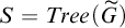 .
.
Claim 5.6 below will verify that
$S $
 is a c.l.c. tree in the sense of Definition 2.4 by providing a computable bound H. The following lemma does the main work, and will also be used later on, such as in the proof of Proposition 8.2 below. Informally, it says that given some subgroup
$U \in \mathcal {W}$
is a c.l.c. tree in the sense of Definition 2.4 by providing a computable bound H. The following lemma does the main work, and will also be used later on, such as in the proof of Proposition 8.2 below. Informally, it says that given some subgroup
$U \in \mathcal {W}$
 , if one declares that
$p\in \widetilde G$
, if one declares that
$p\in \widetilde G$
 has a value
$L\in \mathcal {W}$
has a value
$L\in \mathcal {W}$
 at U, then one can compute for any
$F \in \mathcal {W}$
at U, then one can compute for any
$F \in \mathcal {W}$
 the finite set of possible values of p at F.
Lemma 5.5. Suppose that
$U \in \mathcal {W}$
 is a subgroup and L is a left coset of U. Let
$F \in \mathcal {W}$
is a subgroup and L is a left coset of U. Let
$F \in \mathcal {W}$
 . One can uniformly in
$U, L$
. One can uniformly in
$U, L$
 and F compute a strong index for the finite set
$\mathcal {L}=\{ p(F) \colon \, p \in [S] \, \land \, p(U) = L\}$
and F compute a strong index for the finite set
$\mathcal {L}=\{ p(F) \colon \, p \in [S] \, \land \, p(U) = L\}$
 .
.
To see this, first one computes
$V= F\cdot F^{-1} $
 , so that F is a right coset of the subgroup V. Next one computes
$k=|U \colon U \cap V|$
, so that F is a right coset of the subgroup V. Next one computes
$k=|U \colon U \cap V|$
 , the number of left cosets of
$U \cap V$
, the number of left cosets of
$U \cap V$
 in U. Note that
$\mathcal {L}_0= \{ p(U \cap V) \colon p \in [S] \, \land \, p(U) = L \}$
in U. Note that
$\mathcal {L}_0= \{ p(U \cap V) \colon p \in [S] \, \land \, p(U) = L \}$
 is the set of left cosets of
$U \cap V$
is the set of left cosets of
$U \cap V$
 contained in L. Clearly this set has size k. By searching
$\mathcal {W}$
contained in L. Clearly this set has size k. By searching
$\mathcal {W}$
 until all of its elements have appeared, one can compute a strong index for this set. Next one computes a strong index for the set
$\mathcal {L}_1$
until all of its elements have appeared, one can compute a strong index for this set. Next one computes a strong index for the set
$\mathcal {L}_1$
 of left cosets E of V such that
$C \subseteq E$
of left cosets E of V such that
$C \subseteq E$
 for some
$C \in \mathcal {L}_0$
for some
$C \in \mathcal {L}_0$
 (this uses that, given C, one can compute E). Finally one outputs a strong index for the set
$\{ E F \colon \, E \in \mathcal {L}_1\}$
(this uses that, given C, one can compute E). Finally one outputs a strong index for the set
$\{ E F \colon \, E \in \mathcal {L}_1\}$
 , which equals
$\mathcal {L}$
, which equals
$\mathcal {L}$
 . This proves the lemma.
For the following recall that the computable set
$D\subseteq {\mathbb {N}}$
 is the domain of
$\mathcal {W}$
is the domain of
$\mathcal {W}$
 , and that
$0 \in D$
, and that
$0 \in D$
 denotes a subgroup U. If
$a,b \in D$
denotes a subgroup U. If
$a,b \in D$
 denote left cosets
$L_0,L_1$
denote left cosets
$L_0,L_1$
 of U, then the string
$(a,b) $
of U, then the string
$(a,b) $
 is extended by a path
$p\in [S]$
is extended by a path
$p\in [S]$
 iff
$p(U)= L_0$
iff
$p(U)= L_0$
 and
$p^{-1}(U)= L_1$
and
$p^{-1}(U)= L_1$
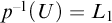 .
.
Claim 5.6. There is a computable binary function H such that, if
$ \sigma $
 is the string
$(a,b)$
is the string
$(a,b)$
 and
$\sigma \in S$
and
$\sigma \in S$
 (so that
$a,b\in D$
(so that
$a,b\in D$
 ), and
$\rho \in S$
), and
$\rho \in S$
 extends
$\sigma $
extends
$\sigma $
 , then
$\rho (i) \le H(\sigma , i)$
, then
$\rho (i) \le H(\sigma , i)$
 for each
$i < |\rho |$
for each
$i < |\rho |$
 . Thus, the tree S is c.l.c. via the parameter
$k=2$
. Thus, the tree S is c.l.c. via the parameter
$k=2$
 .
.
To see this, let
$v=\lfloor i/2 \rfloor $
 . If
$v \not \in D$
. If
$v \not \in D$
 , let
$H(\sigma , i)= i$
, let
$H(\sigma , i)= i$
 . Otherwise, let F be the coset denoted by v. If
$i= 2v$
. Otherwise, let F be the coset denoted by v. If
$i= 2v$
 , let L be the coset denoted by a. If
$i= 2v+1$
, let L be the coset denoted by a. If
$i= 2v+1$
 , let L be the coset denoted by b. Applying Lemma 5.5 to
$U, L, F$
, let L be the coset denoted by b. Applying Lemma 5.5 to
$U, L, F$
 , one can compute
$H(\sigma , i) $
, one can compute
$H(\sigma , i) $
 as the greatest number denoting an element of
$\{ p(F) \colon \, p \in [S] \, \land \, p(U) = L \}$
as the greatest number denoting an element of
$\{ p(F) \colon \, p \in [S] \, \land \, p(U) = L \}$
 .
.
5.1 Understanding the automorphism group via the meet groupoid.
The meet groupoid
$\mathcal {W}(G)$
 might turn out to be a useful tool for studying G, independently of algorithmic considerations. For a general locally compact group G, the group
${Aut}(G)$
might turn out to be a useful tool for studying G, independently of algorithmic considerations. For a general locally compact group G, the group
${Aut}(G)$
 becomes a Polish group via the Braconnier topology, given by the sub-basis of identity neighbourhoods of the form

where K ranges over the compact subsets of G, and U over the identity neighbourhoods of G. As noted in [Reference Caprace and Monod4, Appendix A],
${Aut}(G)$
 with this topology is Polish (assuming that G is countably based). For a t.d.l.c. group G, the following shows that
${Aut}(G)$
with this topology is Polish (assuming that G is countably based). For a t.d.l.c. group G, the following shows that
${Aut}(G)$
 can be viewed as the automorphism group of a countable structure.
Proposition 5.7. Let G be a t.d.l.c. group. The group
${Aut}(G)$
 with the Braconnier topology is topologically isomorphic to
${Aut}(\mathcal {W}(G))$
with the Braconnier topology is topologically isomorphic to
${Aut}(\mathcal {W}(G))$
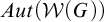 , via the map
$\Gamma $
, via the map
$\Gamma $
 that sends
$\alpha \in {Aut}(G)$
that sends
$\alpha \in {Aut}(G)$
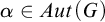 to its action on
$\mathcal {W}(G)$
to its action on
$\mathcal {W}(G)$
 , that is,
$B \mapsto \alpha (B)$
, that is,
$B \mapsto \alpha (B)$
 .
.
Proof. It is clear that
$\Gamma $
 is an injective group homomorphism. To show that
$\Gamma $
is an injective group homomorphism. To show that
$\Gamma $
 is continuous, consider an identity neighbourhood of
${Aut}(\mathcal {W}(G))$
is continuous, consider an identity neighbourhood of
${Aut}(\mathcal {W}(G))$
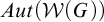 , which we may assume to have the form
$\{\beta \colon \, \beta (A_i)= A_i, i = 1, \ldots , n\}$
, which we may assume to have the form
$\{\beta \colon \, \beta (A_i)= A_i, i = 1, \ldots , n\}$
 where
$A_i \in \mathcal {W}(G)$
where
$A_i \in \mathcal {W}(G)$
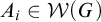 . Let
$U = \bigcap _i A_i A_i^{-1}$
. Let
$U = \bigcap _i A_i A_i^{-1}$
 and
$K= \bigcup A_i$
and
$K= \bigcup A_i$
 . Then
$\alpha \in \mathfrak A(K,U)$
. Then
$\alpha \in \mathfrak A(K,U)$
 implies
$\alpha (A_i) = A_i$
implies
$\alpha (A_i) = A_i$
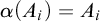 for each i.
It remains to show that
$\Gamma $
 is onto: then, since
${Aut}(G)$
is onto: then, since
${Aut}(G)$
 and
${Aut}(\mathcal {W}(G))$
and
${Aut}(\mathcal {W}(G))$
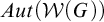 are Polish,
$\Gamma $
are Polish,
$\Gamma $
 is open (see, e.g., [Reference Gao13, Theorem 2.3.3]), and hence a topological group isomorphism. For a direct argument that
$\Gamma $
is open (see, e.g., [Reference Gao13, Theorem 2.3.3]), and hence a topological group isomorphism. For a direct argument that
$\Gamma $
 is onto, see [Reference Nies40, Proposition 9.5]. Given the work already done, here it is easier, however, to derive ontoness using the isomorphism
$\Phi \colon G \to \widetilde G$
is onto, see [Reference Nies40, Proposition 9.5]. Given the work already done, here it is easier, however, to derive ontoness using the isomorphism
$\Phi \colon G \to \widetilde G$
 defined in the proof of the implication “
$\Rightarrow $
defined in the proof of the implication “
$\Rightarrow $
 ” of Theorem 5.1. The map
$\Phi $
” of Theorem 5.1. The map
$\Phi $
 can be defined in the absence of algorithmic considerations. (We can now choose
$D= {\mathbb {N}}$
can be defined in the absence of algorithmic considerations. (We can now choose
$D= {\mathbb {N}}$
 , ignoring the trivial case that G is finite. Furthermore, in the argument below we may ignore the fact that the elements of
$\widetilde G$
, ignoring the trivial case that G is finite. Furthermore, in the argument below we may ignore the fact that the elements of
$\widetilde G$
 are not literally permutations of
${\mathbb {N}}$
are not literally permutations of
${\mathbb {N}}$
 .)
.)
Let
$\Phi ^* \colon {Aut} (G) \to {Aut}(\widetilde G)$
 be the isomorphism induced by
$\Phi \colon G \to \widetilde G$
be the isomorphism induced by
$\Phi \colon G \to \widetilde G$
 , namely,

Let
$\Theta \colon {Aut}(\mathcal {W}(G)) \to {Aut}(\widetilde G)$
 be the 1–1 map given by

for any
$\beta \in {Aut}(\mathcal {W}(G))$
 and
$p \in \widetilde G$
and
$p \in \widetilde G$
 . It is clear that
$\Theta (\beta )(p) \in \widetilde G$
. It is clear that
$\Theta (\beta )(p) \in \widetilde G$
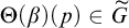 , and
$\Theta (\beta ) $
, and
$\Theta (\beta ) $
 is a continuous automorphism of
$\widetilde G$
is a continuous automorphism of
$\widetilde G$
 . The following diagram summarizes the maps:

To verify that
$\Gamma $
 is onto, we show that
$ \Theta \circ \Gamma =\Phi ^* $
is onto, we show that
$ \Theta \circ \Gamma =\Phi ^* $
 . We use letters
$p,q,r$
. We use letters
$p,q,r$
 for elements of
$\widetilde G$
for elements of
$\widetilde G$
 . Let
$p \in \widetilde G$
. Let
$p \in \widetilde G$
 ,
$\alpha \in {Aut}(G),$
,
$\alpha \in {Aut}(G),$
 and
$C\in \mathcal {W}(G)$
and
$C\in \mathcal {W}(G)$
 be arbitrary. Firstly, note that
$ \Theta (\Gamma (\alpha ))$
be arbitrary. Firstly, note that
$ \Theta (\Gamma (\alpha ))$
 is the map sending p to q where
$q(C)= \alpha (p(\alpha ^{-1}(C)))$
is the map sending p to q where
$q(C)= \alpha (p(\alpha ^{-1}(C)))$
 . Secondly, recall from the proof of Theorem 5.1 that
$\{\Phi ^{-1}(p)\}= \bigcap _U p(U)$
. Secondly, recall from the proof of Theorem 5.1 that
$\{\Phi ^{-1}(p)\}= \bigcap _U p(U)$
 where U ranges through the compact open subgroups of G. So
$\Phi ^*(\alpha )(p)$
where U ranges through the compact open subgroups of G. So
$\Phi ^*(\alpha )(p)$
 is the map r sending C to
$[\bigcap _U \alpha (pU)]C$
is the map r sending C to
$[\bigcap _U \alpha (pU)]C$
 .
.
We verify that
$q=r$
 . If B is a left coset of a subgroup W, we have
$p(B)= [ \bigcap _U pU] B$
. If B is a left coset of a subgroup W, we have
$p(B)= [ \bigcap _U pU] B$
 : both sides are left cosets of W, and we have
$p(B)= p(V)B \supseteq [ \bigcap _U pU] B$
: both sides are left cosets of W, and we have
$p(B)= p(V)B \supseteq [ \bigcap _U pU] B$
 where B is a right coset of a subgroup V. Letting
$B= \alpha ^{-1}(C)$
where B is a right coset of a subgroup V. Letting
$B= \alpha ^{-1}(C)$
 yields

Applying
$\alpha $
 to both sides of this equation shows that
$q(C)=r(C)$
to both sides of this equation shows that
$q(C)=r(C)$
 .
.
6 Computable functions on the set of paths of computable trees.
This section provides preliminaries on computability of functions that are defined on the set of paths of computable trees without leaves. These preliminaries will be used in Section 7 to introduce computable Baire presentations of t.d.l.c. groups, as well as in much of the rest of the article. Most of the content of this section can either be seen as a special case of known results in abstract computable topology, or can be derived from such results. These results stem from the study of computably compact metric spaces; some of them need to be extrapolated to the locally compact setting. They can be found in the recent surveys [Reference Downey and Melnikov8, Reference Iljazović and Kihara20]. However, with the reader in mind who has little background in computability or computable topology, we prefer to provide intuition and elementary proofs for the computability notions and results that are needed later on, rather than referring to such more general results.
Let T be a computable subtree of
${\mathbb {N}}^*$
 without leaves. To define that a function which takes arguments from the potentially uncountable domain
$[T]$
without leaves. To define that a function which takes arguments from the potentially uncountable domain
$[T]$
 is computable, one descends to the countable domain of strings on T, where the usual computability notions work. The first definition, Definition 6.1 below, will apply when we show in Corollary 8.4 that the modular function on a computable presentation of a t.d.l.c. group is computable. As a further example, in Fact 8.6 we will show that given a computable presentation of a t.d.l.c. group via a closed subgroup of
$S_\infty $
is computable, one descends to the countable domain of strings on T, where the usual computability notions work. The first definition, Definition 6.1 below, will apply when we show in Corollary 8.4 that the modular function on a computable presentation of a t.d.l.c. group is computable. As a further example, in Fact 8.6 we will show that given a computable presentation of a t.d.l.c. group via a closed subgroup of
$S_\infty $
 , the function
$m(g,V)$
, the function
$m(g,V)$
 related to the scale function, defined in the introduction, is computable. For the notion of partial computable functions on
${\mathbb {N}}$
related to the scale function, defined in the introduction, is computable. For the notion of partial computable functions on
${\mathbb {N}}$
 , see the remark after Definition 1.3. We assume some standard effective encoding of strings by numbers.
We define what it means to say that
$\Phi : [T] \times {\mathbb {N}} \to {\mathbb {N}}$
 is computable. The intuition is that a partial computable function
$P_\Phi $
is computable. The intuition is that a partial computable function
$P_\Phi $
 represents the behaviour of a so-called oracle Turing machine computing
$\Phi $
represents the behaviour of a so-called oracle Turing machine computing
$\Phi $
 . Given
$f \in [T]$
. Given
$f \in [T]$
 , the machine has the list of the values
$f(0), f(1), f(2), \ldots $
, the machine has the list of the values
$f(0), f(1), f(2), \ldots $
 written on a special “oracle” tape, and attempts to find the value
$\Phi (f, w)$
written on a special “oracle” tape, and attempts to find the value
$\Phi (f, w)$
 via queries of the type “what is the value of
$f(q)$
via queries of the type “what is the value of
$f(q)$
 ?”, where q is determined during the computation. If a string
$\sigma $
?”, where q is determined during the computation. If a string
$\sigma $
 is an initial segment of
$ f$
is an initial segment of
$ f$
 and
$P_\Phi (\sigma ,w) = m$
and
$P_\Phi (\sigma ,w) = m$
 , then with the answers given by
$\sigma $
, then with the answers given by
$\sigma $
 , the machine can find this value m. Clearly any extension
$\tau $
, the machine can find this value m. Clearly any extension
$\tau $
 of
$\sigma $
of
$\sigma $
 will then yield the same value: this is Condition (1). Condition (2) says that sufficiently many queries will lead to an answer. By
$f\! \upharpoonright _{n}$
will then yield the same value: this is Condition (1). Condition (2) says that sufficiently many queries will lead to an answer. By
$f\! \upharpoonright _{n}$
 one denotes the length n initial segment of f.
Definition 6.1. (a) A function
$\Phi : [T] \times {\mathbb {N}} \to {\mathbb {N}}$
 is computable if there is a partial computable function
$P_\Phi $
is computable if there is a partial computable function
$P_\Phi $
 defined on a subset of
$T\times {\mathbb {N}}$
defined on a subset of
$T\times {\mathbb {N}}$
 , with values in
${\mathbb {N}}$
, with values in
${\mathbb {N}}$
 , such that
-
(1) if $\sigma \prec \tau \in T$
, then
$P_\Phi (\sigma , n) = k $
implies
$P_\Phi (\tau , n) = k$
; -
(2) if $f \in [T]$
, then
$\Phi (f, w)= k $
iff there is an n such that
$P_\Phi (f\! \upharpoonright _{n},w) =k$
.




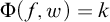

(b) A function
$\Psi : [T] \to {\mathbb {N}}$
 is computable if the function
$\Phi (f, n) = \Psi (f)$
is computable if the function
$\Phi (f, n) = \Psi (f)$
 (which ignores the number input) is computable in the sense above.
By (2),
$\Phi $
 is continuous (where
${\mathbb {N}}$
is continuous (where
${\mathbb {N}}$
 carries the discrete topology).
Example 6.2. Let
$T= {\mathbb {N}}^*$
 . The function
$\Phi (f,n)= \sum _{i=0}^n f(i)$
. The function
$\Phi (f,n)= \sum _{i=0}^n f(i)$
 is computable. The oracle Turing machine, with f “written” on the oracle tape, queries the values of
$f(i)$
is computable. The oracle Turing machine, with f “written” on the oracle tape, queries the values of
$f(i)$
 for
$i=0, \ldots ,n$
for
$i=0, \ldots ,n$
 one by one and adds them.
We next rephrase Definition 6.1 in a form that will matter when we discuss computability for groups where the domain can be of the form
$[T]$
 for any computable tree without leaves. We will need to express that the group operations are computable. In the setting of closed subgroups of
$S_\infty $
for any computable tree without leaves. We will need to express that the group operations are computable. In the setting of closed subgroups of
$S_\infty $
 , this is the case automatically; for the inversion operation, it is due to the particular presentation of
$S_\infty $
, this is the case automatically; for the inversion operation, it is due to the particular presentation of
$S_\infty $
 we chose (Fact 6.6 below).
Given a computable tree R without leaves, there is a computable tree without leaves
$T= R^2$
 such that
$[T]$
such that
$[T]$
 can be canonically identified with
$[R] \times [R]$
can be canonically identified with
$[R] \times [R]$
 : namely, T consists of the initial segments of strings
$\sigma _0 \oplus \sigma _1$
: namely, T consists of the initial segments of strings
$\sigma _0 \oplus \sigma _1$
 where
$\sigma _i \in R$
where
$\sigma _i \in R$
 have the same length. Given this identification, a path f on T can be written as
$\langle f_0, f_1 \rangle $
have the same length. Given this identification, a path f on T can be written as
$\langle f_0, f_1 \rangle $
 where
$f_i \in [R]$
where
$f_i \in [R]$
 .
.
Definition 6.3 (Computable functions on the set of paths).
Let
$R,S,T$
 be computable trees without leaves. A function
$\Phi \colon [T] \to [S] $
be computable trees without leaves. A function
$\Phi \colon [T] \to [S] $
 is called computable if the function
$\widetilde \Phi : [T] \times {\mathbb {N}} \to {\mathbb {N}}$
is called computable if the function
$\widetilde \Phi : [T] \times {\mathbb {N}} \to {\mathbb {N}}$
 given by
$\widetilde \Phi (g, n)= \Phi (g)(n)$
given by
$\widetilde \Phi (g, n)= \Phi (g)(n)$
 is computable in the sense of Definition 6.1. A function
$\Psi \colon [R] \times [R] \to [S] $
is computable in the sense of Definition 6.1. A function
$\Psi \colon [R] \times [R] \to [S] $
 is computable if the function
$\widehat \Psi \colon [R^2] \to [S]$
is computable if the function
$\widehat \Psi \colon [R^2] \to [S]$
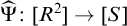 is computable, where
$\widehat \Psi (\langle f_0, f_1 \rangle )= \Psi (f_0, f_1)$
is computable, where
$\widehat \Psi (\langle f_0, f_1 \rangle )= \Psi (f_0, f_1)$
 .
.
It is intuitively clear, and not hard to check from the definitions, that the composition of computable unary functions on sets of paths is again computable. The topology on the space
$[T]$
 is induced by a complete metric: for instance, for
$f \neq g$
is induced by a complete metric: for instance, for
$f \neq g$
 , let
$d(f,g) = 1/n$
, let
$d(f,g) = 1/n$
 where
$n $
where
$n $
 is least such that
$f(n)\neq g(n)$
is least such that
$f(n)\neq g(n)$
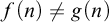 . Taking the usual “
$\varepsilon , \delta $
. Taking the usual “
$\varepsilon , \delta $
 ” definition, one sees that
$\Phi \colon [T] \to [S] $
” definition, one sees that
$\Phi \colon [T] \to [S] $
 is continuous at f if for each k there is n such that for each
$g \in [T]$
is continuous at f if for each k there is n such that for each
$g \in [T]$
 , if
$f\! \upharpoonright _{n} = g\! \upharpoonright _{n}$
, if
$f\! \upharpoonright _{n} = g\! \upharpoonright _{n}$
 then
$\Phi (f)\! \upharpoonright _{k} = \Phi (g) \! \upharpoonright _{k}$
then
$\Phi (f)\! \upharpoonright _{k} = \Phi (g) \! \upharpoonright _{k}$
 . The definitions above can be seen as algorithmic versions of continuity, where one can compute the output
$\Phi (f)$
. The definitions above can be seen as algorithmic versions of continuity, where one can compute the output
$\Phi (f)$
 up to k from a sufficiently long part of the input f.
Notation 6.4. Suppose that a function P is as in Definition 6.1 above, and suppose that for each
$\sigma \in T$
 , the value
$P(\sigma , n)$
, the value
$P(\sigma , n)$
 is only defined for finitely many n. We write
$P(\sigma )= \rho $
is only defined for finitely many n. We write
$P(\sigma )= \rho $
 if
$\rho \in {\mathbb {N}}^*$
if
$\rho \in {\mathbb {N}}^*$
 is the string of maximal length such that
$P(\sigma , n)= \rho (n)$
is the string of maximal length such that
$P(\sigma , n)= \rho (n)$
 for each
$n < |\rho |$
for each
$n < |\rho |$
 .
.
Clearly P as a function on strings is monotonic: if
$\sigma \preceq \rho $
 then
$P(\sigma ) \preceq P(\rho )$
then
$P(\sigma ) \preceq P(\rho )$
 . While P is not partial computable in general, we can think of
$P(\sigma ) $
. While P is not partial computable in general, we can think of
$P(\sigma ) $
 as the eventual output of a finite process depending on computations
$P(\sigma , k)$
as the eventual output of a finite process depending on computations
$P(\sigma , k)$
 converging for larger and larger k.
Remark 6.5. Suppose instead we start by defining a monotonic partial computable function P on strings such that
$\Psi (f)= \bigcup _n \{ P(f\! \upharpoonright _{n}) \colon \, f\! \upharpoonright _{n} \in \mathrm {dom} (P)\}$
 . Then defining the partial computable function
$P(\sigma , n)$
. Then defining the partial computable function
$P(\sigma , n)$
 as
$P(\sigma )(n)$
as
$P(\sigma )(n)$
 for any
$n< P(\sigma )$
for any
$n< P(\sigma )$
 shows that
$\Psi $
shows that
$\Psi $
 is computable in the sense of Definition 6.1. In the algebraic applications below such as Proposition 7.8, we will usually proceed in this way. In fact, the domain of P will usually be a computable set given by a simple combinatorial condition. So the function P is computable in the sense of Definition 1.3.
Recall that in Section 3.1 we introduced a special way of presenting the elements of
$S_\infty $
 as paths
$f = f_0 \oplus f_1$
as paths
$f = f_0 \oplus f_1$
 on a directed tree
${Tree}(S_\infty ) $
on a directed tree
${Tree}(S_\infty ) $
 that keep track of both the permutation
$f_0$
that keep track of both the permutation
$f_0$
 and its inverse
$f_1$
and its inverse
$f_1$
 . For
$f,g \in [{Tree}(S_\infty ) ]$
. For
$f,g \in [{Tree}(S_\infty ) ]$
 , we defined the group operations of
$S_\infty $
, we defined the group operations of
$S_\infty $
 by
$f^{-1} = f_1 \oplus f_0$
by
$f^{-1} = f_1 \oplus f_0$
 and
$g f = (g_0 \circ f_0) \oplus (f_1 \circ g_1 )$
and
$g f = (g_0 \circ f_0) \oplus (f_1 \circ g_1 )$
 .
.
Fact 6.6. The group operations of
$S_\infty $
 are computable.
Proof. We define partial computable monotonic functions
$P_1$
 and
$P_2$
and
$P_2$
 on
${Tree}(S_\infty ) $
on
${Tree}(S_\infty ) $
 and
${Tree}(S_\infty ) ^2$
and
${Tree}(S_\infty ) ^2$
 , respectively, according to Remark 6.5. For the inverse, let
$P_1(\sigma _0 \oplus \sigma _1) = \sigma _1 \oplus \sigma _0$
, respectively, according to Remark 6.5. For the inverse, let
$P_1(\sigma _0 \oplus \sigma _1) = \sigma _1 \oplus \sigma _0$
 , where
$|\sigma _0|=|\sigma _1|$
, where
$|\sigma _0|=|\sigma _1|$
 . For the binary group operation, given strings
$\tau =\tau _0 \oplus \tau _1$
. For the binary group operation, given strings
$\tau =\tau _0 \oplus \tau _1$
 and
$\sigma =\sigma _0 \oplus \sigma _1$
and
$\sigma =\sigma _0 \oplus \sigma _1$
 of the same, even length, let t be greatest such that for each
$r<t$
of the same, even length, let t be greatest such that for each
$r<t$
 ,
$ \rho _0(r):=\tau _0(\sigma _0(r))$
,
$ \rho _0(r):=\tau _0(\sigma _0(r))$
 and
$\rho _1(r):=\sigma _1(\tau _1(s))$
and
$\rho _1(r):=\sigma _1(\tau _1(s))$
 are defined. Let
$P_2(\tau , \sigma ) = \rho _0\oplus \rho _1$
are defined. Let
$P_2(\tau , \sigma ) = \rho _0\oplus \rho _1$
 , a string of length
$2t$
, a string of length
$2t$
 .
.
The following lemma is an algorithmic version of the fact that each continuous function defined on a compact space is uniformly continuous. This is well-known in computable analysis. Here we restrict ourselves to the setting of paths spaces
$[K]$
 that are compact in an effective way (as given by the bound H below).
Lemma 6.7. Suppose that K and
$ S$
 are computable trees without leaves. Suppose further that there is a computable function H such that
$\sigma (i) < H(i)$
are computable trees without leaves. Suppose further that there is a computable function H such that
$\sigma (i) < H(i)$
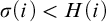 for each
$\sigma \in K$
for each
$\sigma \in K$
 and
$i < |\sigma |$
and
$i < |\sigma |$
 . Let
$\Phi \colon [K]\to [S] $
. Let
$\Phi \colon [K]\to [S] $
 be computable via a partial computable function
$P\colon K \times {\mathbb {N}} \to {\mathbb {N}}$
be computable via a partial computable function
$P\colon K \times {\mathbb {N}} \to {\mathbb {N}}$
 .
.
-
(i) There is a computable function g as follows: for each n,
$$ \begin{align*} \forall \rho \in K \forall i< n \, [|\rho| = g(n) \to P(\rho, i) \text{ is defined}]. \end{align*} $$
Moreover, g is obtained uniformly in K and h.
-
(ii) If $\Phi $
is a bijection then
$\Phi ^{-1}$
is computable, via a partial computable function that is obtained uniformly in
$K,H,S,$
and P.


Intuitively, given the metric on
$[K]$
 discussed above, the function g in (i) computes the “
$\delta $
discussed above, the function g in (i) computes the “
$\delta $
 ” in the definition of uniform continuity from the “
$\varepsilon $
” in the definition of uniform continuity from the “
$\varepsilon $
 ”: if
$\delta = 1/n$
”: if
$\delta = 1/n$
 we have
$\varepsilon = 1/g(n)$
we have
$\varepsilon = 1/g(n)$
 . In computability terms, this means that, to obtain
$n+1$
. In computability terms, this means that, to obtain
$n+1$
 output symbols, we need at most
$g(n)$
output symbols, we need at most
$g(n)$
 input symbols.
Proof. (i) Given
$i \in {\mathbb {N}}$
 , consider the subtree of K consisting of the strings
$\rho $
, consider the subtree of K consisting of the strings
$\rho $
 such that
$P(\rho , i)$
such that
$P(\rho , i)$
 is undefined. If this subtree is infinite, then there is a path
$f \in [K]$
is undefined. If this subtree is infinite, then there is a path
$f \in [K]$
 such that
$\Phi (f)(i)$
such that
$\Phi (f)(i)$
 is undefined, contradiction. Thus for each n a possible value
$g(n)$
is undefined, contradiction. Thus for each n a possible value
$g(n)$
 as above exists. Using the hypotheses on K, given n one can search for the least such value and output it as
$g(n)$
as above exists. Using the hypotheses on K, given n one can search for the least such value and output it as
$g(n)$
 .
.
(ii) To show that
$\Phi ^{-1}$
 is computable, we define a partial computable function
$Q \colon [S] \times {\mathbb {N}} \to {\mathbb {N}}$
is computable, we define a partial computable function
$Q \colon [S] \times {\mathbb {N}} \to {\mathbb {N}}$
 . Clearly
$[S]$
. Clearly
$[S]$
 is compact and
$\Phi ^{-1}$
is compact and
$\Phi ^{-1}$
 is continuous. Hence there is a computable function h with
$h(t) \ge t$
is continuous. Hence there is a computable function h with
$h(t) \ge t$
 for each t as follows: given
$s \in {\mathbb {N}}$
for each t as follows: given
$s \in {\mathbb {N}}$
 , for each
$\rho \in K$
, for each
$\rho \in K$
 of length
$g(h(s))$
of length
$g(h(s))$
 , the values
$P(\rho ,i)$
, the values
$P(\rho ,i)$
 for
$i< h(s)$
for
$i< h(s)$
 together determine
$\rho \! \upharpoonright _{s}$
together determine
$\rho \! \upharpoonright _{s}$
 . For a string
$\beta \in S$
. For a string
$\beta \in S$
 of length
$h(s)$
of length
$h(s)$
 and
$k<s$
and
$k<s$
 , define
$Q(\beta ,k)= \rho (k)$
, define
$Q(\beta ,k)= \rho (k)$
 where
$\rho \in K$
where
$\rho \in K$
 is a string of length
$g(h(s))$
is a string of length
$g(h(s))$
 with
$P(\rho ,i) = \beta (i)$
with
$P(\rho ,i) = \beta (i)$
 for each
$i< h(s)$
for each
$i< h(s)$
 . It is easy to verify that Q shows that
$\Phi ^{-1}$
. It is easy to verify that Q shows that
$\Phi ^{-1}$
 is computable, and that Q is obtained uniformly in the given data. For a proof in a more general setting see [Reference Downey and Melnikov9, Theorem 4.2.48].
The rest of this section discusses computable functions on the set of paths of c.l.c. trees. Given such a tree T, recall from Definition 2.5 that by
$\mathcal {K}_u$
 we denote the compact open subset of
$[T]$
we denote the compact open subset of
$[T]$
 with code number
$u\in {\mathbb {N}}$
with code number
$u\in {\mathbb {N}}$
 . That is, u is the strong index for a set of strings
$\{\alpha _1, \ldots , \alpha _r \} \subseteq T$
. That is, u is the strong index for a set of strings
$\{\alpha _1, \ldots , \alpha _r \} \subseteq T$
 such that
$\mathcal {K}_u= \bigcup _{i\le r} [\alpha _i]_T$
such that
$\mathcal {K}_u= \bigcup _{i\le r} [\alpha _i]_T$
 . If there is more than one tree under discussion, we will write
$\mathcal {K}_u^T$
. If there is more than one tree under discussion, we will write
$\mathcal {K}_u^T$
 for the subset of
$[T]$
for the subset of
$[T]$
 with code number u. First, we establish a useful interaction between computable functions
$[T]\to [S]$
with code number u. First, we establish a useful interaction between computable functions
$[T]\to [S]$
 and such sets. This generalizes Lemma 2.6(ii) where
$\Phi $
and such sets. This generalizes Lemma 2.6(ii) where
$\Phi $
 is the identity function.
Lemma 6.8. Let T and S be c.l.c. trees. Suppose a function
$\Phi \colon [T]\to [S] $
 is computable via a partial computable function
$P_\Phi $
is computable via a partial computable function
$P_\Phi $
 . Given code numbers
$u, w$
. Given code numbers
$u, w$
 , one can decide whether
$\Phi (\mathcal {K}^T_u) \subseteq \mathcal {K}^S_w$
, one can decide whether
$\Phi (\mathcal {K}^T_u) \subseteq \mathcal {K}^S_w$
 .
.
Proof. Suppose that u is a strong index for the set of strings
$\{\alpha _1, \ldots , \alpha _r \} \subseteq T$
 , and w is a strong index for the set of strings
$\{\beta _1, \ldots , \beta _s \} \subseteq S$
, and w is a strong index for the set of strings
$\{\beta _1, \ldots , \beta _s \} \subseteq S$
 . Let K be the subtree of T consisting of the prefixes, or extensions, of some
$\alpha _i$
. Let K be the subtree of T consisting of the prefixes, or extensions, of some
$\alpha _i$
 . Clearly one can uniformly obtain a computable bound H for this K as in Lemma 6.7. Let
$n= \max _i |\beta _i|$
. Clearly one can uniformly obtain a computable bound H for this K as in Lemma 6.7. Let
$n= \max _i |\beta _i|$
 . Let
$N= g(n)$
. Let
$N= g(n)$
 be the length computed from n through Lemma 6.7. Then
$\Phi (\mathcal {K}^T_u) \subseteq \mathcal {K}^S_w$
be the length computed from n through Lemma 6.7. Then
$\Phi (\mathcal {K}^T_u) \subseteq \mathcal {K}^S_w$
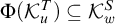 if and only if for each
$\alpha \in K$
if and only if for each
$\alpha \in K$
 of length N, there is an i such that
$P_\Phi (\alpha ) \succeq \beta _i$
of length N, there is an i such that
$P_\Phi (\alpha ) \succeq \beta _i$
 . By Lemma 6.7, this condition is decidable.
To prove Proposition 7.8 below, we will need a criterion on whether, given a computable subtree S of a c.l.c. tree T (where S potentially has leaves), the maximally pruned subtree of S with the same set of paths is computable.
Proposition 6.9. Let T be a c.l.c. tree such that only the root is infinitely branching. Let
$S $
 be a computable subtree of T, and suppose that there is a uniformly computable dense sequence
$(f_i)_{i\in {\mathbb {N}}}$
be a computable subtree of T, and suppose that there is a uniformly computable dense sequence
$(f_i)_{i\in {\mathbb {N}}}$
 in
$[S]$
in
$[S]$
 . Then the tree
$\widetilde S= \{\sigma \colon [\sigma ]_S \neq \emptyset \}$
. Then the tree
$\widetilde S= \{\sigma \colon [\sigma ]_S \neq \emptyset \}$
 is decidable. (It follows that
$\widetilde S$
is decidable. (It follows that
$\widetilde S$
 is c.l.c. Of course,
$[\widetilde S] = [S]$
is c.l.c. Of course,
$[\widetilde S] = [S]$
 .)
.)
Proof. Given a string
$\sigma \in T$
 , if
$\sigma = \emptyset $
, if
$\sigma = \emptyset $
 then
$\sigma \in \widetilde S$
then
$\sigma \in \widetilde S$
 . Assuming
$\sigma \neq \emptyset $
. Assuming
$\sigma \neq \emptyset $
 , we can compute the least
$t\in {\mathbb {N}}$
, we can compute the least
$t\in {\mathbb {N}}$
 such that either
$\sigma \prec f_t$
such that either
$\sigma \prec f_t$
 , or
$\rho \not \in S$
, or
$\rho \not \in S$
 for each
$\rho \in T$
for each
$\rho \in T$
 of length t such that
$ \rho \succeq \sigma $
of length t such that
$ \rho \succeq \sigma $
 ; the latter condition can be decided by the hypotheses on T. Clearly
$\sigma \in \widetilde S$
; the latter condition can be decided by the hypotheses on T. Clearly
$\sigma \in \widetilde S$
 iff the former condition holds.
7 Defining computably t.d.l.c. groups via Baire presentations.
This section spells out the third type of computable presentations of t.d.l.c. groups described in Section 1.4, Type B, which generalises Type S. We call them computable Baire presentations.
It is well-known that each zero-dimensional Polish space X is homeomorphic to the path space
$[T]$
 for some tree
$T \subseteq {\mathbb {N}}^*$
for some tree
$T \subseteq {\mathbb {N}}^*$
 (see [Reference Kechris22, I.7.8]). Clearly X is locally compact if and only if for each
$f \in [T]$
(see [Reference Kechris22, I.7.8]). Clearly X is locally compact if and only if for each
$f \in [T]$
 there is an n such that the tree above
$f\! \upharpoonright _{n}$
there is an n such that the tree above
$f\! \upharpoonright _{n}$
 is finitely branching. Considering the set of prefix minimal strings
$\sigma \in T$
is finitely branching. Considering the set of prefix minimal strings
$\sigma \in T$
 such that
$[\sigma ]_T$
such that
$[\sigma ]_T$
 is compact, it is easy to see that we may replace T by a tree such that only the root can have infinitely many successors. So in our effective setting, it is natural to work with a domain of the presentation that has the form
$[T]$
is compact, it is easy to see that we may replace T by a tree such that only the root can have infinitely many successors. So in our effective setting, it is natural to work with a domain of the presentation that has the form
$[T]$
 for a c.l.c. tree T, and require that the group operations on
$[T]$
for a c.l.c. tree T, and require that the group operations on
$[T]$
 be computable. (In fact, while the previous types of computable presentation were group-specific, in the present setting the same approach would work for other types of algebraic structure defined on
$[T]$
be computable. (In fact, while the previous types of computable presentation were group-specific, in the present setting the same approach would work for other types of algebraic structure defined on
$[T]$
 .) We will show in Theorem 7.6 that the resulting notion of computably t.d.l.c. group is equivalent to the previous ones.
Despite this equivalence, as presentations, computable Baire presentations offer more flexibility than the first type (Type S), which relied on closed subgroups of
$S_\infty $
 . This will be evidenced by our proofs that some algebraic groups over local fields, such as
$\operatorname {\mathrm {SL}}_n({\mathbb {Q}}_p)$
. This will be evidenced by our proofs that some algebraic groups over local fields, such as
$\operatorname {\mathrm {SL}}_n({\mathbb {Q}}_p)$
 , are computable.
Definition 7.1. A computable Baire presentation is a topological group of the form
$H= ([T], {Mult}, {Inv})$
 such that
-
(1) T is c.l.c. as defined in Definition 2.4;
-
(2) ${Mult}\colon [T] \times [T] \to [T]$
and
${Inv} \colon [T] \to [T]$
are computable.


We say that a t.d.l.c. group G is computably t.d.l.c. (via a Baire presentation) if
$G \cong H$
 for such a group H.
We verify next that for profinite groups and for countable discrete groups, our notion of computable presentability (type B) for t.d.l.c. groups coincides with the notions established in the literature. First we provide the formal definition of a computable profinite presentation.
Definition 7.2 (La Roche [Reference La Roche49] and Smith [Reference Smith52]).
A computable profinite presentation of a profinite group G is a uniformly computable sequence of strong indices of finite groups
$A_i$
 and finite surjective maps
$\phi _i: A_i \rightarrow A_{i-1}$
and finite surjective maps
$\phi _i: A_i \rightarrow A_{i-1}$
 such that
$G = \varprojlim _i (A_i, \phi _i)$
such that
$G = \varprojlim _i (A_i, \phi _i)$
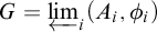 .
.
Proposition 7.3. Given a computable profinite presentation of G, one can effectively obtain a computable Baire presentation of G.
Proof. We use the notation of Definition 7.2. Let
$n_i= | A_i|$
 . By the hypotheses one can effectively identify the elements of
$ A_i$
. By the hypotheses one can effectively identify the elements of
$ A_i$
 with
$\{ 0, \ldots , n_i-1\}$
with
$\{ 0, \ldots , n_i-1\}$
 . Let
. Let

It is clear from the hypotheses that T is c.l.c. via
$k=0$
 (Definition 2.4). To show that the binary group operation
${Mult}$
(Definition 2.4). To show that the binary group operation
${Mult}$
 on
$[T]$
on
$[T]$
 is computable, for strings
$\sigma _0, \sigma _1$
is computable, for strings
$\sigma _0, \sigma _1$
 on T of the same length
$k+1$
on T of the same length
$k+1$
 , let
$P_2 (\sigma _0, \sigma _1)$
, let
$P_2 (\sigma _0, \sigma _1)$
 be the unique string
$\tau \in T$
be the unique string
$\tau \in T$
 of length
$k+1$
of length
$k+1$
 such that in
$\mathcal {A}_k$
such that in
$\mathcal {A}_k$
 one has
$\sigma _0(k) \sigma _1(k) = \tau (k)$
one has
$\sigma _0(k) \sigma _1(k) = \tau (k)$
 . The inversion operation
${Inv}$
. The inversion operation
${Inv}$
 on
$[T]$
on
$[T]$
 is computable by a similar argument.
We will see in Proposition B.7 that the converse holds as well. So, for profinite groups our definition of computably t.d.l.c. group coincides with the existing one. We note that Smith [Reference Smith52] already obtained this equivalence, using a different terminology.
Proposition 7.4. A discrete group G has a computable presentation in the usual sense of Definition 1.4 if and only if it has a computable Baire presentation.
Proof. “
$\Rightarrow $
 ”: Let the computable set
$D\subseteq {\mathbb {N}}$
”: Let the computable set
$D\subseteq {\mathbb {N}}$
 be the domain of the computable presentation. For the computable Baire presentation, we take the c.l.c. tree

and the operations canonically defined on
$[T_G]$
 via partial computable functions that only regard the first entry of the oracle strings.
“
$\Leftarrow $
 ”: By Theorem 7.6 proved shortly below, G has a computable presentation via a meet groupoid. It now suffices to invoke Example 4.8.
By Fact 6.6, each computable presentation of G as a closed subgroup of
$S_\infty $
 (Definition 3.3) is a computable Baire presentation. Lemma 3.5 showed that for a computable presentation as a closed subgroup of
$S_\infty $
(Definition 3.3) is a computable Baire presentation. Lemma 3.5 showed that for a computable presentation as a closed subgroup of
$S_\infty $
 , the group theoretic operations on compact open sets are algorithmic. In the more general setting of computable Baire presentations, a weak version of Lemma 3.5 still holds. Recall from Definition 2.7 that given a c.l.c. tree T, by
$E_T$
, the group theoretic operations on compact open sets are algorithmic. In the more general setting of computable Baire presentations, a weak version of Lemma 3.5 still holds. Recall from Definition 2.7 that given a c.l.c. tree T, by
$E_T$
 we denote the set of minimal code numbers u such that
$\mathcal {K}_u$
we denote the set of minimal code numbers u such that
$\mathcal {K}_u$
 is compact.
Lemma 7.5. Let G be computably t.d.l.c. via a computable Baire presentation
$([T], {Mult}, {Inv})$
 .
.
(i) There is a computable function
$ I \colon E_T \to E_T$
 such that for each
$u \in E_T$
such that for each
$u \in E_T$
 , one has
$\mathcal {K}_{I(u)} = (\mathcal {K}_u)^{-1}$
, one has
$\mathcal {K}_{I(u)} = (\mathcal {K}_u)^{-1}$
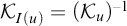 .
.
(ii) Given
$u,v,w \in E_T$
 , one can decide whether
$\mathcal {K}_u \mathcal {K}_v \subseteq \mathcal {K}_w$
, one can decide whether
$\mathcal {K}_u \mathcal {K}_v \subseteq \mathcal {K}_w$
 .
.
Proof. (i) By Lemma 6.8 one can decide whether
$\mathcal {K}_u\subseteq (\mathcal {K}_w)^{-1}$
 . The equality
$\mathcal {K}_u= (\mathcal {K}_w)^{-1}$
. The equality
$\mathcal {K}_u= (\mathcal {K}_w)^{-1}$
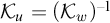 is equivalent to
$\mathcal {K}_u\subseteq (\mathcal {K}_w)^{-1}\, \land \, \mathcal {K}_w\subseteq (\mathcal {K}_u)^{-1}$
is equivalent to
$\mathcal {K}_u\subseteq (\mathcal {K}_w)^{-1}\, \land \, \mathcal {K}_w\subseteq (\mathcal {K}_u)^{-1}$
 . So one lets
$I(u)$
. So one lets
$I(u)$
 be the least index v such that this equality holds.
(ii) Let
$\widetilde T$
 be the tree of initial segments of strings of the form
$\sigma _0 \oplus \sigma _1$
be the tree of initial segments of strings of the form
$\sigma _0 \oplus \sigma _1$
 , where
$\sigma _0, \sigma _1 \in T$
, where
$\sigma _0, \sigma _1 \in T$
 have the same length. Then
$\widetilde T$
have the same length. Then
$\widetilde T$
 is a c.l.c. tree,
$[\widetilde T]$
is a c.l.c. tree,
$[\widetilde T]$
 is naturally homeomorphic to
$[T] \times [T]$
is naturally homeomorphic to
$[T] \times [T]$
 , and
${Mult}$
, and
${Mult}$
 can be seen as a computable function
$[\widetilde T ] \to [T]$
can be seen as a computable function
$[\widetilde T ] \to [T]$
 . Now one applies Lemma 6.8.
As discussed at the beginning of this section, the following adds a further equivalent condition to Theorem 5.1.
Theorem 7.6. A group G is computably t.d.l.c. via a Baire presentation
$\Leftrightarrow $

G is computably t.d.l.c. via a meet groupoid.
From a presentation of G of one type, one can effectively obtain a presentation of G of the other type.
Proof. “
$\Leftarrow $
 ”: This follows from the corresponding implication in Theorem 5.1.
“
$\Rightarrow $
 ”: We build a Haar computable copy
$\mathcal {W}$
”: We build a Haar computable copy
$\mathcal {W}$
 of the meet groupoid
$\mathcal {W}(G)$
of the meet groupoid
$\mathcal {W}(G)$
 as required in Definition 4.6. By Lemma 7.5, one can decide whether
$u \in E_T$
as required in Definition 4.6. By Lemma 7.5, one can decide whether
$u \in E_T$
 is the code number (Definition 2.5) of a subgroup. Furthermore, one can decide whether
$B= \mathcal {K}_w $
is the code number (Definition 2.5) of a subgroup. Furthermore, one can decide whether
$B= \mathcal {K}_w $
 is a left coset of a subgroup
$U= \mathcal {K}_u$
is a left coset of a subgroup
$U= \mathcal {K}_u$
 : this holds iff
$BU \subseteq B$
: this holds iff
$BU \subseteq B$
 and
$B^{-1} B \subseteq U$
and
$B^{-1} B \subseteq U$
 , and the latter two conditions are decidable by Lemma 7.5. Similarly, one can decide whether B is a right coset of U.
It follows that the set
$V= \{ w \in E_T \colon \, \mathcal {K}_w \text { is a coset}\}$
 can be obtained via an existential quantification over a computable binary relation; in other words, V is r.e. A basic fact from computability theory states that from a description of V as an r.e. set one can uniformly obtain a computable set
$\widetilde D \subseteq {\mathbb {N}}^+$
can be obtained via an existential quantification over a computable binary relation; in other words, V is r.e. A basic fact from computability theory states that from a description of V as an r.e. set one can uniformly obtain a computable set
$\widetilde D \subseteq {\mathbb {N}}^+$
 and a computable bijection
$\theta \colon \widetilde D \to V$
and a computable bijection
$\theta \colon \widetilde D \to V$
 . (Here
$\widetilde D$
. (Here
$\widetilde D$
 is the set of “stages” at which new elements are enumerated into V; one can assume that at each stage
$n \in \widetilde D$
is the set of “stages” at which new elements are enumerated into V; one can assume that at each stage
$n \in \widetilde D$
 exactly one element
$\theta (n)$
exactly one element
$\theta (n)$
 is enumerated.) Write
$A_n = \mathcal {K}_{\theta (n)}$
is enumerated.) Write
$A_n = \mathcal {K}_{\theta (n)}$
 for
$n\in \widetilde D$
for
$n\in \widetilde D$
 , and
$A_0 = \emptyset $
, and
$A_0 = \emptyset $
 .
.
The domain of
$\mathcal {W}$
 is
$D = \widetilde D \cup \{0\}$
is
$D = \widetilde D \cup \{0\}$
 . By Lemma 2.6 the intersection operation on
$\mathcal {W}$
. By Lemma 2.6 the intersection operation on
$\mathcal {W}$
 is computable, i.e., there is a computable binary function c on
${\mathbb {N}}$
is computable, i.e., there is a computable binary function c on
${\mathbb {N}}$
 such that
$A_{c(n,k)} =A_n \cap A_k$
such that
$A_{c(n,k)} =A_n \cap A_k$
 . Given
$n,k \in {\mathbb {N}}-\{0\}$
. Given
$n,k \in {\mathbb {N}}-\{0\}$
 one can decide whether
$A_n$
one can decide whether
$A_n$
 is a right coset of the same subgroup that
$A_k$
is a right coset of the same subgroup that
$A_k$
 is a left coset of. In that case, one can compute the number r such that
$A_r= A_n\cdot A_k$
is a left coset of. In that case, one can compute the number r such that
$A_r= A_n\cdot A_k$
 : one uses that
$A_r$
: one uses that
$A_r$
 is the unique coset C such that
-
(a) $A_nA_k \subseteq C$
, and -
(b) C is a right coset of the same subgroup that $A_k$
is a right coset of.


As in the corresponding implication in the proof of Theorem 5.1, for subgroups
$U,V$
 , one can compute
$|U \colon U \cap V|$
, one can compute
$|U \colon U \cap V|$
 by finding in
$\mathcal {W}$
by finding in
$\mathcal {W}$
 further and further distinct left cosets of
$U \cap V$
further and further distinct left cosets of
$U \cap V$
 contained in U, until their union reaches U. The latter condition is decidable.
Notation 7.7. Given a computable Baire presentation G, by
$\mathcal {W}_{\text {comp}} (G)$
 we denote the computable copy of
$\mathcal {W}(G)$
we denote the computable copy of
$\mathcal {W}(G)$
 obtained in the proof above.
Proposition 7.8. Let p be a prime, and let
$n \ge 2$
 . Let
${\mathbb {Q}}_p$
. Let
${\mathbb {Q}}_p$
 and
$F_p((t))$
and
$F_p((t))$
 denote the rings of p-adic numbers, and Laurent series over
$\mathbb F_p$
denote the rings of p-adic numbers, and Laurent series over
$\mathbb F_p$
 , respectively. The t.d.l.c. groups
$\operatorname {\mathrm {SL}}_n({\mathbb {Q}}_p)$
, respectively. The t.d.l.c. groups
$\operatorname {\mathrm {SL}}_n({\mathbb {Q}}_p)$
 and
$\operatorname {\mathrm {SL}}_n(\mathbb F_p((t)))$
and
$\operatorname {\mathrm {SL}}_n(\mathbb F_p((t)))$
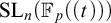 have computable Baire presentations.
Proof. We provide the proof for the groups
$\operatorname {\mathrm {SL}}_n({\mathbb {Q}}_p)$
 , and then indicate the changes that are necessary for the groups
$\operatorname {\mathrm {SL}}_n(\mathbb F_p((t)))$
, and then indicate the changes that are necessary for the groups
$\operatorname {\mathrm {SL}}_n(\mathbb F_p((t)))$
 . We begin by giving a computable Baire presentation of
${\mathbb {Q}}_p$
. We begin by giving a computable Baire presentation of
${\mathbb {Q}}_p$
 as a ring.
Let Q be the tree of strings
$\sigma \in {\mathbb {N}}^*$
 such that all the entries, except possibly the first, are among
$\{0, \ldots , p-1\}$
such that all the entries, except possibly the first, are among
$\{0, \ldots , p-1\}$
 , and
$r0 \not \preceq \sigma $
, and
$r0 \not \preceq \sigma $
 for each
$r>0$
for each
$r>0$
 . Clearly Q is c.l.c. via
$k=1$
. Clearly Q is c.l.c. via
$k=1$
 (Definition 2.4). We think of a string
$r \hat {\ } \sigma \in Q$
(Definition 2.4). We think of a string
$r \hat {\ } \sigma \in Q$
 as denoting the rational number
$p^{-r} n_\sigma \in {\mathbb {Z}}[1/p]$
as denoting the rational number
$p^{-r} n_\sigma \in {\mathbb {Z}}[1/p]$
 , where
$n_\sigma $
, where
$n_\sigma $
 is the natural number that has
$\sigma $
is the natural number that has
$\sigma $
 as a p-ary expansion, written in reverse order:

The condition that
$r0 \not \preceq \sigma $
 for each
$r>0$
for each
$r>0$
 expresses that p does not divide
$n_\sigma $
expresses that p does not divide
$n_\sigma $
 unless
$r=0$
unless
$r=0$
 . Let
$\sigma , \tau $
. Let
$\sigma , \tau $
 be strings over
$\{0, \ldots , p-1\}$
be strings over
$\{0, \ldots , p-1\}$
 of the same length
$\ell $
of the same length
$\ell $
 . By
$\sigma + \tau $
. By
$\sigma + \tau $
 we denote the string
$\rho $
we denote the string
$\rho $
 of the same length
$\ell $
of the same length
$\ell $
 such that
$n_\rho = n_\sigma + n_\tau \mod p^\ell $
such that
$n_\rho = n_\sigma + n_\tau \mod p^\ell $
 . By
$\sigma \cdot \tau $
. By
$\sigma \cdot \tau $
 we denote the string
$\rho $
we denote the string
$\rho $
 of length
$2\ell $
of length
$2\ell $
 such that
$n_\rho = n_\sigma n_\tau \mod p^{2\ell }$
such that
$n_\rho = n_\sigma n_\tau \mod p^{2\ell }$
 .
.
We now provide partial computable functions
$P, P_1, P_2, P_3$
 according to Remark 6.5 that are defined on computable subsets of the trees Q or
$Q^2$
according to Remark 6.5 that are defined on computable subsets of the trees Q or
$Q^2$
 , in order to show that various operations on
$[Q]$
, in order to show that various operations on
$[Q]$
 are computable according to Definition 6.3. For a string of the form
$r\sigma $
are computable according to Definition 6.3. For a string of the form
$r\sigma $
 let
let

where
$k\in {\mathbb {N}} $
 is maximal such that
$k \le r$
is maximal such that
$k \le r$
 and
$0^k\preceq \sigma $
and
$0^k\preceq \sigma $
 , and
$\tau $
, and
$\tau $
 is the rest, i.e.,
$0^k \tau = \sigma $
is the rest, i.e.,
$0^k \tau = \sigma $
 . To show the computability of the function
$q \to -q$
. To show the computability of the function
$q \to -q$
 , let
, let
To show that the addition operation is computable, if
$r, s \in {\mathbb {N}}$
 and
$\sigma , \tau $
and
$\sigma , \tau $
 are strings such that
$r+ |\tau | = s + |\sigma |$
are strings such that
$r+ |\tau | = s + |\sigma |$
 , let
, let

To show that the multiplication operation is computable, let

$P_2$
 and
$P_3$
and
$P_3$
 are the correct functions because, say for
$r\le s$
are the correct functions because, say for
$r\le s$
 , in
${\mathbb {Z}}[1/p]$
, in
${\mathbb {Z}}[1/p]$
 one has
$p^{-r} n_\sigma + p^{-s}n_\tau = p^{-s}(n_{0^{s-r}\sigma }+n_\tau )$
one has
$p^{-r} n_\sigma + p^{-s}n_\tau = p^{-s}(n_{0^{s-r}\sigma }+n_\tau )$
 and
$p^{-r} n_\sigma p^{-s}n_\tau = p^{-2s}n_{0^{s-r}\sigma }n_\tau $
and
$p^{-r} n_\sigma p^{-s}n_\tau = p^{-2s}n_{0^{s-r}\sigma }n_\tau $
 .
.
We next provide a computable Baire presentation
$([T], {Mult}, {Inv})$
 of
$\operatorname {\mathrm {SL}}_n({\mathbb {Q}}_p)$
of
$\operatorname {\mathrm {SL}}_n({\mathbb {Q}}_p)$
 as in Definition 7.1. Let T be the c.l.c. tree that is an
$n^2$
as in Definition 7.1. Let T be the c.l.c. tree that is an
$n^2$
 -fold “power” of Q. More precisely,
$T = \{ \sigma \colon \forall i < n^2 \, [ \sigma ^i \in Q]\}$
-fold “power” of Q. More precisely,
$T = \{ \sigma \colon \forall i < n^2 \, [ \sigma ^i \in Q]\}$
 , where
$\sigma ^i$
, where
$\sigma ^i$
 is the string of entries of
$\sigma $
is the string of entries of
$\sigma $
 in positions of the form
$\ell n^2 + i$
in positions of the form
$\ell n^2 + i$
 for some
$\ell ,i \in {\mathbb {N}}$
for some
$\ell ,i \in {\mathbb {N}}$
 . Clearly,
$[T]$
. Clearly,
$[T]$
 is c.l.c. via
$k= n^2$
is c.l.c. via
$k= n^2$
 , and T can be naturally identified with the matrix algebra
$M_n({\mathbb {Q}}_p)$
, and T can be naturally identified with the matrix algebra
$M_n({\mathbb {Q}}_p)$
 . By the computability of the ring operations on
${\mathbb {Q}}_p$
. By the computability of the ring operations on
${\mathbb {Q}}_p$
 as verified above, the matrix product is computable as a function
$[T] \times [T]\to [T]$
as verified above, the matrix product is computable as a function
$[T] \times [T]\to [T]$
 , and the function
$\det \colon [T] \to [Q]$
, and the function
$\det \colon [T] \to [Q]$
 is computable.
Note that for any c.l.c. trees T and R, any computable path f of R, and any computable function
$\Phi \colon [T]\to [R]$
 , there is a computable subtree
$S $
, there is a computable subtree
$S $
 of T such that
$[S]$
of T such that
$[S]$
 equals the pre-image
$\Phi ^{-1}(f)$
equals the pre-image
$\Phi ^{-1}(f)$
 . (In the language of computable analysis, the pre-image is effectively closed.) To see this, suppose that
$\Phi $
. (In the language of computable analysis, the pre-image is effectively closed.) To see this, suppose that
$\Phi $
 is computable according to Definition 6.3 via a partial computable function L taking pairs in
$T\times {\mathbb {N}}$
is computable according to Definition 6.3 via a partial computable function L taking pairs in
$T\times {\mathbb {N}}$
 to
${\mathbb {N}}$
to
${\mathbb {N}}$
 . Let S consist of the strings
$\sigma \in T$
. Let S consist of the strings
$\sigma \in T$
 of length t such that t steps of the attempted computations
$L(\sigma ,k) $
of length t such that t steps of the attempted computations
$L(\sigma ,k) $
 don’t yield a contradiction to the hypothesis that the output of the oracle Turing machine equals f. More formally,

In our setting, applying this to the function
$\det \colon [T] \to [Q]$
 and the path
$f = 01000\ldots $
and the path
$f = 01000\ldots $
 that denotes
$1 \in {\mathbb {Q}}_p$
that denotes
$1 \in {\mathbb {Q}}_p$
 , we obtain a computable subtree S of T such that
$[S]$
, we obtain a computable subtree S of T such that
$[S]$
 can be identified with
$SL_n({\mathbb {Q}}_p)$
can be identified with
$SL_n({\mathbb {Q}}_p)$
 .
.
It is well-known that
$SL_n({\mathbb {Z}}[1/p])$
 is dense in
$SL_n({\mathbb {Q}}_p)$
is dense in
$SL_n({\mathbb {Q}}_p)$
 . This is a special case of strong approximation for algebraic groups (see [Reference Platonov and Rapinchuk45, Chapter 7]), but can also be seen in an elementary way using Gaussian elimination. The paths on S corresponding to matrices in
$SL_n({\mathbb {Z}}[1/p])$
. This is a special case of strong approximation for algebraic groups (see [Reference Platonov and Rapinchuk45, Chapter 7]), but can also be seen in an elementary way using Gaussian elimination. The paths on S corresponding to matrices in
$SL_n({\mathbb {Z}}[1/p])$
 are precisely the ones that are
$0$
are precisely the ones that are
$0$
 from some point on. Clearly there is a computable listing
$(f_i)$
from some point on. Clearly there is a computable listing
$(f_i)$
 of the set of such paths. So by Proposition 6.9 one can replace S by a c.l.c. tree
$\widetilde S$
of the set of such paths. So by Proposition 6.9 one can replace S by a c.l.c. tree
$\widetilde S$
 such that
$[\widetilde S] = [S]$
such that
$[\widetilde S] = [S]$
 .
.
To obtain a computable Baire presentation based on
$\widetilde S$
 , note that matrix multiplication on
$[\widetilde S]$
, note that matrix multiplication on
$[\widetilde S]$
 is computable as the restriction of matrix multiplication on
$[T]$
is computable as the restriction of matrix multiplication on
$[T]$
 . To define the matrix inversion operation
${Inv}$
. To define the matrix inversion operation
${Inv}$
 , we use the fact that the inverse of a matrix with determinant
$1$
, we use the fact that the inverse of a matrix with determinant
$1$
 equals its adjugate matrix; the latter can be obtained by computing determinants on minors.
Next we treat
$SL_n(\mathbb F_p((t)))$
 . To give a Baire presentation of
$\mathbb F_p((t))$
. To give a Baire presentation of
$\mathbb F_p((t))$
 as a ring, we use the same tree Q as above, but now think of a string
$r\sigma $
as a ring, we use the same tree Q as above, but now think of a string
$r\sigma $
 as representing the finite Laurent series
$t^{-r} n_\sigma \in {\mathbb {Z}}[1/p]$
as representing the finite Laurent series
$t^{-r} n_\sigma \in {\mathbb {Z}}[1/p]$
 , where
$n_\sigma = \sum _{i< |\sigma |} t^i \sigma (i)$
, where
$n_\sigma = \sum _{i< |\sigma |} t^i \sigma (i)$
 . For strings
$\sigma , \tau $
. For strings
$\sigma , \tau $
 over
$\{0, \ldots , p-1\}$
over
$\{0, \ldots , p-1\}$
 and of the same length
$\ell $
and of the same length
$\ell $
 , by
$\sigma + \tau $
, by
$\sigma + \tau $
 we denote the string
$\rho $
we denote the string
$\rho $
 of length
$\ell $
of length
$\ell $
 such that
$n_\rho = n_\sigma + n_\tau \mod p^\ell $
such that
$n_\rho = n_\sigma + n_\tau \mod p^\ell $
 . By
$\sigma \cdot \tau $
. By
$\sigma \cdot \tau $
 we denote the string
$\rho $
we denote the string
$\rho $
 of length
$2\ell $
of length
$2\ell $
 such that
$n_\rho \equiv n_\sigma n_\tau \mod t^{2\ell }$
such that
$n_\rho \equiv n_\sigma n_\tau \mod t^{2\ell }$
 . Now the ring operations are computable via the partial computable functions defined as for the case of
${\mathbb {Q}}_p$
. Now the ring operations are computable via the partial computable functions defined as for the case of
${\mathbb {Q}}_p$
 , but with the new interpretation of the symbols “
$+$
, but with the new interpretation of the symbols “
$+$
 ” and “
$\cdot $
” and “
$\cdot $
 ” as operations on strings. The remainder of the proof didn’t use any particulars about the computable Baire presentation of the ring
${\mathbb {Q}}_p$
” as operations on strings. The remainder of the proof didn’t use any particulars about the computable Baire presentation of the ring
${\mathbb {Q}}_p$
 , besides the fact that the path denoting
$1$
, besides the fact that the path denoting
$1$
 is computable; this carries over to the present case. It is known that
$SL_n(\mathbb F_p(t))$
is computable; this carries over to the present case. It is known that
$SL_n(\mathbb F_p(t))$
 , the group of matrices over finite Laurent series with determinant 1, forms a dense subgroup of
$SL_n(\mathbb F_p((t)))$
, the group of matrices over finite Laurent series with determinant 1, forms a dense subgroup of
$SL_n(\mathbb F_p((t)))$
 , so from here on we can argue as before.
8 More on the equivalences of notions of computable presentation.
Theorem 5.1 and its extension Theorem 7.6 showed that our various notions of computable presentation of a t.d.l.c. group are equivalent. This section obtains extra information from the proofs of these equivalences. The main result of the section, Theorem 8.2 will show that, given a computable Baire presentation
$ ([T], {Mult}, {Inv})$
 of a t.d.l.c. group G, one can effectively obtain a computable presentation of G via a closed subgroup
$\widetilde G$
of a t.d.l.c. group G, one can effectively obtain a computable presentation of G via a closed subgroup
$\widetilde G$
 of
$S_\infty $
of
$S_\infty $
 , with an isomorphism
$\Phi \colon [T] \to \widetilde G$
, with an isomorphism
$\Phi \colon [T] \to \widetilde G$
 so that both
$\Phi $
so that both
$\Phi $
 and
$\Phi ^{-1}$
and
$\Phi ^{-1}$
 are computable. The presentation based on a closed subgroup of
$S_\infty $
are computable. The presentation based on a closed subgroup of
$S_\infty $
 can be seen as an “improved” computable Baire presentation. For instance, the group operations on compact open subsets of
$\widetilde G$
can be seen as an “improved” computable Baire presentation. For instance, the group operations on compact open subsets of
$\widetilde G$
 are fully computable by Lemma 3.5, while in the general case we only have the weaker form Lemma 7.5.
The section then proceeds to two applications of Theorem 8.2: computability of the modular function and computability of Cayley–Abels graphs. For a compactly generated t.d.l.c. group G, its Cayley–Abels graphs are generalisations of the usual Cayley graphs in the setting of a (discrete) finitely generated group. We will show that each Cayley–Abels graph can be interpreted via first-order formulas with parameters in the meet groupoid of G. The interpretation is constructed in such a way that if G is computably t.d.l.c., the graphs are computable in a uniform way.
In Section 8.3 we apply Theorem 8.2 to obtain an upper bound on the computational complexity of the scale function. As a further application, in Section 10 we will obtain an equivalent criterion on whether a t.d.l.c. group G has a unique computable Baire presentation up to computable group homeomorphism: any two Haar computable copies of its meet groupoid
$\mathcal {W}(G)$
 are computably isomorphic. This is useful because uniqueness of a computable presentation is easier to show for countable structures. In Theorem 10.6 we will apply the criterion to show the uniqueness of a computable Baire presentation for the additive groups of the p-adic integers and the p-adic numbers, as well as for
${\mathbb {Z}} \ltimes {\mathbb {Q}}_p$
are computably isomorphic. This is useful because uniqueness of a computable presentation is easier to show for countable structures. In Theorem 10.6 we will apply the criterion to show the uniqueness of a computable Baire presentation for the additive groups of the p-adic integers and the p-adic numbers, as well as for
${\mathbb {Z}} \ltimes {\mathbb {Q}}_p$
 .
.
Besides the computability theoretic concepts introduced in Section 6, we will need a fact on continuous, open functions on the set of paths of c.l.c. trees. It deduces the computability of such a function from the hypothesis that its action on the compact open sets is computable in terms of their code numbers. Similar to the results in Section 6, this is a special case of a result in the field of computable topology (see [Reference Downey and Melnikov8, Lemma 2.13]). However, we prefer to present a short, elementary proof.
Proposition 8.1. Let T and
$ S$
 be c.l.c. trees (see Definition 2.4), and let the function
$\Phi \colon [T]\to [S]$
be c.l.c. trees (see Definition 2.4), and let the function
$\Phi \colon [T]\to [S]$
 be continuous and open. Suppose that there is a computable function
$f\colon {\mathbb {N}} \to {\mathbb {N}}$
be continuous and open. Suppose that there is a computable function
$f\colon {\mathbb {N}} \to {\mathbb {N}}$
 such that for each code number u one has
$\Phi (\mathcal {K}_u^T)=\mathcal {K}_{f(u)}^S$
such that for each code number u one has
$\Phi (\mathcal {K}_u^T)=\mathcal {K}_{f(u)}^S$
 . Then
(i)
$\Phi $
 is computable;
(ii) if
$\Phi $
 is a bijection then
$\Phi ^{-1}$
is a bijection then
$\Phi ^{-1}$
 is computable as well.
Proof. (i) To show that
$\Phi $
 is computable, we define a partial computable function
$P_\Phi $
is computable, we define a partial computable function
$P_\Phi $
 on T with values in S according to Remark 6.5. Given
$\sigma \in T$
on T with values in S according to Remark 6.5. Given
$\sigma \in T$
 such that
$[\sigma ]_T$
such that
$[\sigma ]_T$
 is compact, compute u such that
$\mathcal {K}^T_u = [\sigma ]_T$
is compact, compute u such that
$\mathcal {K}^T_u = [\sigma ]_T$
 . Let
$\{\beta _1, \ldots , \beta _s \} \subseteq S$
. Let
$\{\beta _1, \ldots , \beta _s \} \subseteq S$
 be the finite set with strong index
$f(u)$
be the finite set with strong index
$f(u)$
 . Let
$\eta =P_\Phi (\sigma )$
. Let
$\eta =P_\Phi (\sigma )$
 be the longest common initial segment of the strings
$\beta _i$
be the longest common initial segment of the strings
$\beta _i$
 . Note that with the standard ultrametric on
$[S]$
. Note that with the standard ultrametric on
$[S]$
 , the set
$[\eta ]_S$
, the set
$[\eta ]_S$
 is a closed ball centred at any element of
$\mathcal {K}_{f(u)}^S$
is a closed ball centred at any element of
$\mathcal {K}_{f(u)}^S$
 , with the same diameter as
$\mathcal {K}_{f(u)}^S$
, with the same diameter as
$\mathcal {K}_{f(u)}^S$
 . So if
$\sigma \preceq \tau \in T$
. So if
$\sigma \preceq \tau \in T$
 then
$[P_\Phi (\sigma )]_S \supseteq [P_\Phi (\tau )]_S$
then
$[P_\Phi (\sigma )]_S \supseteq [P_\Phi (\tau )]_S$
 . This shows that
$P_\Phi $
. This shows that
$P_\Phi $
 is monotonic. Since
$\Phi $
is monotonic. Since
$\Phi $
 is continuous, one has

as required.
(ii) By Lemma 2.6 applied to S, there is a computable function g that is “inverse” to f in the sense such that for each v such that
$\mathcal {K}_v^S$
 is compact, one has
$\Phi ^{-1}(\mathcal {K}_v^S)=\mathcal {K}_{g(v)}^T$
is compact, one has
$\Phi ^{-1}(\mathcal {K}_v^S)=\mathcal {K}_{g(v)}^T$
 . Now one applies (i) to
$\Phi ^{-1}$
. Now one applies (i) to
$\Phi ^{-1}$
 and g.
8.1 Computable action on the meet groupoid.
Towards the main result of this section, let
$G= ([T], {Mult}, {Inv})$
 be a computable Baire presentation of a t.d.l.c. group. Let
$\mathcal {W} $
be a computable Baire presentation of a t.d.l.c. group. Let
$\mathcal {W} $
 be the computable copy of
$ \mathcal {W}(G)$
be the computable copy of
$ \mathcal {W}(G)$
 with domain D given by the proof of “
$\Rightarrow $
with domain D given by the proof of “
$\Rightarrow $
 ” in Theorem 7.6. Recall (Notation 7.7) that we write
$\mathcal {W}= \mathcal {W}_{\text {comp}}(G)$
” in Theorem 7.6. Recall (Notation 7.7) that we write
$\mathcal {W}= \mathcal {W}_{\text {comp}}(G)$
 . Let
$\widetilde G = \mathcal {G}_{\text {comp}} (\mathcal {W})$
. Let
$\widetilde G = \mathcal {G}_{\text {comp}} (\mathcal {W})$
 as in Definition 5.2. Let
$\Phi \colon G \to \widetilde G$
as in Definition 5.2. Let
$\Phi \colon G \to \widetilde G$
 be given by the action
$(g,A) \mapsto gA$
be given by the action
$(g,A) \mapsto gA$
 ; see near the end of the proof of the implication “
$\Leftarrow $
; see near the end of the proof of the implication “
$\Leftarrow $
 ” of Theorem 5.1.
Theorem 8.2. Let
$G, \mathcal {W}$
 ,
$\widetilde G$
,
$\widetilde G$
 and the homeomorphism
$\Phi \colon G \to \widetilde G$
and the homeomorphism
$\Phi \colon G \to \widetilde G$
 be as defined above.
-
(i) $\Phi $
is computable, with a computable inverse. -
(ii) The action $[T] \times D \to D$
, given by
$(g,A) \mapsto gA$
, is computable.


Proof. (i) Write
$S = {Tree}(\widetilde G) $
 . By Proposition 8.1 it suffices to show that there is a computable function f such that
$\Phi (\mathcal {K}_u^T)=\mathcal {K}_{f(u)}^S$
. By Proposition 8.1 it suffices to show that there is a computable function f such that
$\Phi (\mathcal {K}_u^T)=\mathcal {K}_{f(u)}^S$
 for each code number u.
We may assume that
$\mathcal {K}_u^T$
 is of the form
$A \cap B$
is of the form
$A \cap B$
 where
$A $
where
$A $
 is a left coset of a subgroup U such that B is a right coset of U: trivially a group G is the union of the right cosets of any given subgroup; hence such sets form a basis of the topology of G. And by Lemma 2.6, given a general compact set
$\mathcal {K}_w^T$
is a left coset of a subgroup U such that B is a right coset of U: trivially a group G is the union of the right cosets of any given subgroup; hence such sets form a basis of the topology of G. And by Lemma 2.6, given a general compact set
$\mathcal {K}_w^T$
 one can effectively write it as a finite union of sets of this form.
If
$\mathcal {K}_u^T$
 is of the form
$A \cap B$
is of the form
$A \cap B$
 as above, we have

Given any
$F \in \mathcal {W}$
 , by Lemma 5.5 we can compute bounds on
$p(F)$
, by Lemma 5.5 we can compute bounds on
$p(F)$
 and
$p^{-1}(F)$
and
$p^{-1}(F)$
 whenever
$p \in \Phi (\mathcal {K}_u^T)$
whenever
$p \in \Phi (\mathcal {K}_u^T)$
 , letting
$L=A$
, letting
$L=A$
 and
$L=B,$
and
$L=B,$
 respectively. Recall the set
$E_T$
respectively. Recall the set
$E_T$
 from Definition 2.7, and recall from the proof of “
$\Rightarrow $
from Definition 2.7, and recall from the proof of “
$\Rightarrow $
 ” in Theorem 7.6 that
$\theta \colon D \to E_T$
” in Theorem 7.6 that
$\theta \colon D \to E_T$
 is a 1–1 function with range the minimal code numbers of compact open cosets in G; we write
$A_n$
is a 1–1 function with range the minimal code numbers of compact open cosets in G; we write
$A_n$
 for the coset with code number
$\theta (n)$
for the coset with code number
$\theta (n)$
 , and often identify
$A_n$
, and often identify
$A_n$
 with n. Suppose that
$U = A_n$
with n. Suppose that
$U = A_n$
 . Let
$f(u)$
. Let
$f(u)$
 be a strong index for the finite set of strings
$\beta \in S$
be a strong index for the finite set of strings
$\beta \in S$
 of length
$2n+2$
of length
$2n+2$
 such that
-
(a) $A_{\beta (2n)} = A$
and
$A_{\beta (2n+1)} = B$
; -
(b) for $r< 2n$
of the form
$2i$
,
$\beta (r) $
is less than the bound on
$p(F)$
given by Lemma 5.5 where
$L=A$
and
$F= A_i$
; -
(c) for $r< 2n$
of the form
$2i+1$
,
$\beta (r) $
is less than the bound on
$p^{-1} (F)$
given by Lemma 5.5 where
$L= B$
and
$F= A_i$
.


Then
$\Phi (\mathcal {K}_u^T) = \mathcal {K}^S_{f(u)}$
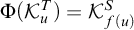 as required.
(ii) Formally, by Definition 6.3, the left action is computable iff
$\Phi $
 is computable. Informally speaking, we use an oracle Turing machine that has as an oracle a path g on
$[T]$
is computable. Informally speaking, we use an oracle Turing machine that has as an oracle a path g on
$[T]$
 , and as an input an
$A \in \mathcal {W}$
, and as an input an
$A \in \mathcal {W}$
 . If A is a left coset of a subgroup V, it outputs the left coset B of V such that it can find a string
$\sigma \prec g$
. If A is a left coset of a subgroup V, it outputs the left coset B of V such that it can find a string
$\sigma \prec g$
 with
$[\sigma ]_TA \subseteq B$
with
$[\sigma ]_TA \subseteq B$
 .
.
Note (ii) implies that the right action is also computable, using that
$Ag = (g^{-1}A^{-1})^{-1}$
 and inversion is computable both in G and in
$\mathcal {W}$
and inversion is computable both in G and in
$\mathcal {W}$
 .
.
We apply the theorem to obtain a computable version of the open mapping theorem for t.d.l.c. groups (Remark 1.2) in the case of a bijection. (This shows that the inverse of
$\Phi $
 in (i) of the theorem is in fact automatically computable.)
Corollary 8.3. Let
$G,H$
 be t.d.l.c. groups given by computable Baire presentations, and let
$\Psi \colon G \to H$
be t.d.l.c. groups given by computable Baire presentations, and let
$\Psi \colon G \to H$
 be a computable bijection that is a group homomorphism. Then
$\Psi ^{-1}$
be a computable bijection that is a group homomorphism. Then
$\Psi ^{-1}$
 is computable.
Proof. Since
$\Psi $
 is a continuous group isomorphism, it is open by the open mapping theorem. Fix a compact open subgroup U of G. Then
$V= \Psi (U)$
is a continuous group isomorphism, it is open by the open mapping theorem. Fix a compact open subgroup U of G. Then
$V= \Psi (U)$
 is a compact open subgroup of H. Let
${\langle {a_i}\rangle }_{i\in {\mathbb {N}}}$
is a compact open subgroup of H. Let
${\langle {a_i}\rangle }_{i\in {\mathbb {N}}}$
 be a uniformly computable sequence of left coset representatives of U in G. To obtain this, fix an effective numbering
${\langle {\sigma _k}\rangle }_{k\in {\mathbb {N}}}$
be a uniformly computable sequence of left coset representatives of U in G. To obtain this, fix an effective numbering
${\langle {\sigma _k}\rangle }_{k\in {\mathbb {N}}}$
 of
${Tree}(G) $
of
${Tree}(G) $
 , and let
$ b_k $
, and let
$ b_k $
 be a uniformly computable path of
${Tree}(G) $
be a uniformly computable path of
${Tree}(G) $
 extending
$\sigma _k$
extending
$\sigma _k$
 . Let
${\langle {a_i}\rangle }_{i\in {\mathbb {N}}}$
. Let
${\langle {a_i}\rangle }_{i\in {\mathbb {N}}}$
 be the subsequence of
${\langle {b_k}\rangle }_{k\in {\mathbb {N}}}$
be the subsequence of
${\langle {b_k}\rangle }_{k\in {\mathbb {N}}}$
 obtained by deleting
$b_k$
obtained by deleting
$b_k$
 if
$b_k U = b_\ell U$
if
$b_k U = b_\ell U$
 for some
$\ell < k$
for some
$\ell < k$
 . Now
${\langle {\Psi (a_i)}\rangle }_{i\in {\mathbb {N}}}$
. Now
${\langle {\Psi (a_i)}\rangle }_{i\in {\mathbb {N}}}$
 is a uniformly computable sequence of left coset representatives for V in H. By (ii) of the theorem, the sequences of (code numbers for) compact open cosets
$K_i:= a_i U$
is a uniformly computable sequence of left coset representatives for V in H. By (ii) of the theorem, the sequences of (code numbers for) compact open cosets
$K_i:= a_i U$
 and
$S_i:= \Psi (K_i)= \Psi (a_i)V$
and
$S_i:= \Psi (K_i)= \Psi (a_i)V$
 are uniformly computable.
By Lemma 6.7(ii), we have a “local” computable inverse
$\Theta _i \colon S_i \to K_i$
 of the restriction
$\Psi _i \! \upharpoonright _{K_i}$
of the restriction
$\Psi _i \! \upharpoonright _{K_i}$
 , given by uniformly partial computable functions
$Q_i$
, given by uniformly partial computable functions
$Q_i$
 with arguments in
${Tree}(H) \times {\mathbb {N}}$
with arguments in
${Tree}(H) \times {\mathbb {N}}$
 , according to Definition 6.3. To show that
$\Psi ^{-1}$
, according to Definition 6.3. To show that
$\Psi ^{-1}$
 is computable, intuitively, using a path
$h \in H$
is computable, intuitively, using a path
$h \in H$
 as an oracle, compute the i such that
$h \in S_i$
as an oracle, compute the i such that
$h \in S_i$
 , and output
$\Theta _i(h)$
, and output
$\Theta _i(h)$
 . More formally, define a partial computable function Q as follows: given
$\sigma \in {Tree}(H) $
. More formally, define a partial computable function Q as follows: given
$\sigma \in {Tree}(H) $
 and
$n \in {\mathbb {N}}$
and
$n \in {\mathbb {N}}$
 , search for i such that
$[\sigma ]_{{Tree}(H) } \subseteq S_i$
, search for i such that
$[\sigma ]_{{Tree}(H) } \subseteq S_i$
 . If i is found, simulate the computation for
$Q_i(\sigma ,n)$
. If i is found, simulate the computation for
$Q_i(\sigma ,n)$
 and give the corresponding output.
8.2 Modular function and Cayley–Abels graphs.
In Section 1.2 we discussed the modular function
$\Delta \colon G \to {\mathbb {R}}^+$
 . As our second application of Theorem 8.2, we show that for any computable presentation, the modular function is computable.
Corollary 8.4. Let G be computably t.d.l.c. via a Baire presentation
$([T], {Mult}, {Inv})$
 . Then the modular function
$\Delta \colon [T] \to {\mathbb {Q}}^+$
. Then the modular function
$\Delta \colon [T] \to {\mathbb {Q}}^+$
 is computable.
Proof. We use the notation of Theorem 8.2. Let
$V \in \mathcal {W}$
 be any subgroup. Given
$g \in [T]$
be any subgroup. Given
$g \in [T]$
 , by (ii) of the theorem compute
$A=g V$
, by (ii) of the theorem compute
$A=g V$
 . Compute
$U = A \cdot A^{-1} \in \mathcal {W}$
. Compute
$U = A \cdot A^{-1} \in \mathcal {W}$
 such that
$A $
such that
$A $
 is a right coset of U, and hence
$A = Ug$
is a right coset of U, and hence
$A = Ug$
 . For any left Haar measure
$\mu $
. For any left Haar measure
$\mu $
 on G, we have

By Remark 4.7 we can choose
$\mu $
 computable; so this suffices to determine
$\Delta (g)$
computable; so this suffices to determine
$\Delta (g)$
 .
.
Our third application of the theorem is to show computability of the Cayley–Abels graphs, discussed in the introduction. Let G be a t.d.l.c. group that is compactly generated, i.e., algebraically generated by a compact subset. Then there is a compact open subgroup U, and a set
$S = \{ s_1, \ldots , s_k\} \subseteq G$
 such that
$S = S^{-1}$
such that
$S = S^{-1}$
 and
$U \cup S$
and
$U \cup S$
 algebraically generates G. The Cayley–Abels graph
$ \Gamma _{S,U}= (V_{S,U}, E_{S,U})$
algebraically generates G. The Cayley–Abels graph
$ \Gamma _{S,U}= (V_{S,U}, E_{S,U})$
 of G is given as follows. The vertex set
$V_{S,U}$
of G is given as follows. The vertex set
$V_{S,U}$
 is the set
$L(U) $
is the set
$L(U) $
 of left cosets of U, and the edge relation is

Some background and original references are given in Section 5 of [Reference Willis60]. For more detailed background see [Reference Krön and Möller24, Section 2] or Part 4 of [Reference Wesolek57]. If G is discrete (and hence finitely generated), then
$\Gamma _{S,\{1\}}$
 is the usual Cayley graph for the generating set S. Any two Cayley–Abels graphs of G with the shortest path distance are quasi-isometric. Here a quasi-isometry between metric spaces
$(X,d_X)$
is the usual Cayley graph for the generating set S. Any two Cayley–Abels graphs of G with the shortest path distance are quasi-isometric. Here a quasi-isometry between metric spaces
$(X,d_X)$
 and
$(Y,d_Y)$
and
$(Y,d_Y)$
 is a map
$\psi \colon X\to Y$
is a map
$\psi \colon X\to Y$
 such that for some
$k,c \in {\mathbb {N}}^+$
such that for some
$k,c \in {\mathbb {N}}^+$
 , one has
$\forall y \in Y \exists x \in X \, d_Y(\psi (x), y ) \le c$
, one has
$\forall y \in Y \exists x \in X \, d_Y(\psi (x), y ) \le c$
 , and
$\forall x, x' \in X [ \frac 1 k d_X(x,x')-c \le d_Y(\psi (x), \psi (x')) \le k d_X(x, x') +c] $
, and
$\forall x, x' \in X [ \frac 1 k d_X(x,x')-c \le d_Y(\psi (x), \psi (x')) \le k d_X(x, x') +c] $
 . Also see [Reference Krön and Möller24, Definition 3] or [Reference Wesolek57].
Theorem 8.5. Suppose that G is computably t.d.l.c. and compactly generated.
-
(i) Each Cayley–Abels graph $\Gamma _{S,U}$
of G has a computable copy
$\mathcal {L}$
. Given a Haar computable copy
$\mathcal {W}$
of the meet groupoid
$\mathcal {W}(G)$
, one can obtain
$\mathcal {L}$
effectively from
$U \in \mathcal {W}$
and the left cosets
$C_i = s_iU$
, where
$\{ s_1, \ldots , s_k\} $
is as above. -
(ii) If $\Gamma _{S',V}$
is another Cayley–Abels graph obtained as above, then
$\Gamma _{S,U}$
and
$\Gamma _{S',V}$
are computably quasi-isometric. -
(iii) Given a computable Baire presentation of G based on a tree $[T]$
, let
$\mathcal {W}= \mathcal {W}_{\text {comp}}(G)$
be the computable copy of its meet groupoid as in Notation 7.7. Then the left action
$[T] \times \mathcal {L} \to \mathcal {L}$
is also computable.


Proof. (i) For the domain of the computable copy
$\mathcal {L}$
 , we take the computable set of left cosets of U. We show that the edge relation is first-order definable from the parameters in such a way that it can be verified to be computable as well.
Let
$V_i = C_i \cdot C_i^{-1}$
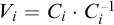 so that
$C_i$
so that
$C_i$
 is a right coset of
$V_i$
is a right coset of
$V_i$
 . Let
$V = U \cap \bigcap _{1 \le i \le k} V_i$
. Let
$V = U \cap \bigcap _{1 \le i \le k} V_i$
 . To first-order define
$E_\Gamma $
. To first-order define
$E_\Gamma $
 in
$\mathcal {W}$
in
$\mathcal {W}$
 with the given parameters, the idea is to replace the elements g in the definition of
$E_\Gamma $
with the given parameters, the idea is to replace the elements g in the definition of
$E_\Gamma $
 by left cosets P of V, since they are sufficiently accurate approximations to g. It is easy to verify that
$\langle A, B \rangle \in E_\Gamma \Leftrightarrow $
by left cosets P of V, since they are sufficiently accurate approximations to g. It is easy to verify that
$\langle A, B \rangle \in E_\Gamma \Leftrightarrow $


where
$L(U)$
 denotes the set of left cosets of a subgroup U: For the implication “
$\Leftarrow $
denotes the set of left cosets of a subgroup U: For the implication “
$\Leftarrow $
 ”, let
$g\in P$
”, let
$g\in P$
 ; then we have
$A = gU$
; then we have
$A = gU$
 and
$B = gs_i U$
and
$B = gs_i U$
 . For the implication “
$\Rightarrow $
. For the implication “
$\Rightarrow $
 ”, given
$A = gU$
”, given
$A = gU$
 and
$B= gs_i U$
and
$B= gs_i U$
 , let
$P\in L(V)$
, let
$P\in L(V)$
 such that
$g \in P$
such that
$g \in P$
 .
.
We verify that the edge relation
$E_\Gamma $
 is computable. Since
$\mathcal {W}$
is computable. Since
$\mathcal {W}$
 is Haar computable, by the usual enumeration argument we can obtain a strong index for the set of left cosets of V contained in A. Given P in this set and
$i \le k$
is Haar computable, by the usual enumeration argument we can obtain a strong index for the set of left cosets of V contained in A. Given P in this set and
$i \le k$
 , the left coset
$Q= Q_{P,i}$
, the left coset
$Q= Q_{P,i}$
 of
$V_i$
of
$V_i$
 in the expression above is unique and can be determined effectively. So we can test whether
$\langle A, B \rangle \in E_\Gamma $
in the expression above is unique and can be determined effectively. So we can test whether
$\langle A, B \rangle \in E_\Gamma $
 by trying all P and all
$i\le k$
by trying all P and all
$i\le k$
 and checking whether
$B = Q_{P,i} \cdot C_i$
and checking whether
$B = Q_{P,i} \cdot C_i$
 .
.
It is clear from the argument that we obtained
$\mathcal {L}$
 effectively from the parameters U and
$C_i$
effectively from the parameters U and
$C_i$
 .
.
(ii) First suppose that
$V \subseteq U$
 . There is a computable map
$\psi \colon L(U) \to L(V)$
. There is a computable map
$\psi \colon L(U) \to L(V)$
 such that
$\psi (A) \subseteq A$
such that
$\psi (A) \subseteq A$
 for each
$A\in L(U)$
for each
$A\in L(U)$
 . The proof of [Reference Krön and Möller24, Theorem 2
${}^{+}$
. The proof of [Reference Krön and Möller24, Theorem 2
${}^{+}$
 ] shows that
$\psi \colon \Gamma _{S,U} \to \Gamma _{S',V}$
] shows that
$\psi \colon \Gamma _{S,U} \to \Gamma _{S',V}$
 is a quasi-isometry. In the general case, let
$R\subseteq G$
is a quasi-isometry. In the general case, let
$R\subseteq G$
 be a finite symmetric set such that
$(U \cap V) \cup R$
be a finite symmetric set such that
$(U \cap V) \cup R$
 algebraically generates G. There are computable quasi-isometries
$\phi \colon \Gamma _{S,U} \to \Gamma _{R, U \cap V}$
algebraically generates G. There are computable quasi-isometries
$\phi \colon \Gamma _{S,U} \to \Gamma _{R, U \cap V}$
 and
$\psi \colon \Gamma _{S',V} \to \Gamma _{R, U \cap V}$
and
$\psi \colon \Gamma _{S',V} \to \Gamma _{R, U \cap V}$
 as above. There is a computable quasi-isometry
$\theta : \Gamma _{R, U \cap V} \to \Gamma _{S',V}$
as above. There is a computable quasi-isometry
$\theta : \Gamma _{R, U \cap V} \to \Gamma _{S',V}$
 inverting
$\psi $
inverting
$\psi $
 : given a vertex
$y\in L(U \cap V)$
: given a vertex
$y\in L(U \cap V)$
 , let
$x= \theta (y)$
, let
$x= \theta (y)$
 be a vertex in
$L( V)$
be a vertex in
$L( V)$
 such that
$\psi (x)$
such that
$\psi (x)$
 is at distance at most c from y, where c is a constant for
$\psi $
is at distance at most c from y, where c is a constant for
$\psi $
 as above. Then
$\theta \circ \phi $
as above. Then
$\theta \circ \phi $
 is a quasi-isometry as required. (iii) follows immediately from Theorem 8.2(ii).
8.3 Algorithmic properties of the scale function.
In Section 1.2 we discussed the scale function
$s \colon G \to {\mathbb {N}}^+$
 for a t.d.l.c. group G, introduced by Willis [Reference Willis58]. Recall that for a compact open subgroup V of G and an element
$g\in G$
for a t.d.l.c. group G, introduced by Willis [Reference Willis58]. Recall that for a compact open subgroup V of G and an element
$g\in G$
 one defines
$m(g,V) = |gVg^{-1}\colon V \cap gVg^{-1}|$
one defines
$m(g,V) = |gVg^{-1}\colon V \cap gVg^{-1}|$
 , and
, and

Willis proved that the scale function is continuous, where
${\mathbb {N}}^+$
 carries the discrete topology. He introduced the relation that a compact open subgroup V is tidy for g, and showed that this condition is equivalent to being minimizing for g in the sense that
$s(g)= m(g,V)$
carries the discrete topology. He introduced the relation that a compact open subgroup V is tidy for g, and showed that this condition is equivalent to being minimizing for g in the sense that
$s(g)= m(g,V)$
 . Möller [Reference Möller36] used graph theoretic methods to show that V is minimizing for g if and only if
$ m(g^k, V) = m(g,V)^k$
. Möller [Reference Möller36] used graph theoretic methods to show that V is minimizing for g if and only if
$ m(g^k, V) = m(g,V)^k$
 for each
$k\in {\mathbb {N}}$
for each
$k\in {\mathbb {N}}$
 . He also derived the “spectral radius formula”: for any compact open subgroup U, one has
$s(g)= \lim _k m(g^k, U)^{1/k}$
. He also derived the “spectral radius formula”: for any compact open subgroup U, one has
$s(g)= \lim _k m(g^k, U)^{1/k}$
 .
.
For this section, fix a computable Baire presentation
$([T], {Mult}, {Inv})$
 of a t.d.l.c. group G as in Definition 7.1. Let
$\mathcal {W} = \mathcal {W}_{\text {comp}}(G)$
of a t.d.l.c. group G as in Definition 7.1. Let
$\mathcal {W} = \mathcal {W}_{\text {comp}}(G)$
 be the Haar computable copy of
$ \mathcal {W}(G)$
be the Haar computable copy of
$ \mathcal {W}(G)$
 given by Notation 7.7. Recall that the domain of
$\mathcal {W}$
given by Notation 7.7. Recall that the domain of
$\mathcal {W}$
 is a computable set D. Via
$\mathcal {W}$
is a computable set D. Via
$\mathcal {W}$
 , we can identify compact open cosets of G with natural numbers. The following is immediate from Theorems 7.6 and 8.2.
Fact 8.6. The function
$m \colon [T] \times D \to D$
 (defined to be
$0$
(defined to be
$0$
 if the second argument is not a subgroup) is computable.
Here and in Section 10, we will study whether the scale function, seen as a function
$s\colon [T]\to {\mathbb {N}}$
 , is computable in the sense of Definition 6.1. We note that neither Möller’s spectral radius formula, nor the tidying procedure of Willis (see again [Reference Willis60]) allow to compute the scale in our sense. The scale is computable iff one can algorithmically decide whether a subgroup is minimizing.
Fact 8.7. The scale function on
$[T]$
 is computable iff the following function
$\Phi $
is computable iff the following function
$\Phi $
 is computable in the sense of Definition 6.1: if
$g \in [T] $
is computable in the sense of Definition 6.1: if
$g \in [T] $
 and V is a compact open subgroup of G, then
$\Phi (g,V)=1$
and V is a compact open subgroup of G, then
$\Phi (g,V)=1$
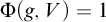 if V is minimizing for g; otherwise
$\Phi (g,V)=0$
if V is minimizing for g; otherwise
$\Phi (g,V)=0$
 .
.
Proof. “
$\Rightarrow $
 ”: An oracle Turing machine with oracle g searches for the first V that is minimizing for g, and outputs
$m(g,V)$
”: An oracle Turing machine with oracle g searches for the first V that is minimizing for g, and outputs
$m(g,V)$
 .
.
“
$\Leftarrow $
 ”: For oracle g, given input V check whether
$m(g,V) = s(g)$
”: For oracle g, given input V check whether
$m(g,V) = s(g)$
 . If so output
$1$
. If so output
$1$
 , otherwise
$0$
, otherwise
$0$
 .
.
We next provide a fact restricting the complexity of the scale function. We say that a function
$\Psi : [T] \to {\mathbb {N}}$
 is computably approximable from above if there is a computable function
$\Theta : [T] \times {\mathbb {N}} \to {\mathbb {N}}$
is computably approximable from above if there is a computable function
$\Theta : [T] \times {\mathbb {N}} \to {\mathbb {N}}$
 such that
$\Theta (f ,r) \ge \Theta (f ,r+1)$
such that
$\Theta (f ,r) \ge \Theta (f ,r+1)$
 for each
$f\in [T],r\in {\mathbb {N}}$
for each
$f\in [T],r\in {\mathbb {N}}$
 , and
, and

Fact 8.8. The scale function is computably approximable from above.
Proof. Let
$\Theta (f,r)$
 be the minimum value of
$m(f,s)$
be the minimum value of
$m(f,s)$
 over all
$s \le r$
over all
$s \le r$
 .
.
The following example is well-known [Reference Willis60, Example 2]; we include it to show that our framework is adequate as a general background for case-based approaches to computability for t.d.l.c. groups used in earlier works.
Example 8.9 (with Stephan Tornier).
For
$d \ge 3$
 , the scale function on
${Aut}(T_d)$
, the scale function on
${Aut}(T_d)$
 in the computable presentation of Example 3.4 is computable.
Proof. An automorphism g of
$T_d$
 has exactly one of three types (see [Reference Figà-Talamanca and Nebbia12]):
-
(1) g fixes a vertex v: then $s(g)= 1$
because g preserves the stabilizer of v, which is a compact open subgroup. -
(2) g inverts an edge: then $s(g)= 1$
because g preserves the set-wise stabilizer of the set of endpoints of this edge. -
(3) g translates along an axis (a subset of $T_d$
that is a homogeneous tree of degree
$2$
): then
$s(g) = (d-1)^\ell $
where
$\ell $
is the length. To see this, for
$\ell =1$
one uses as a minimizing subgroup the compact open subgroup of automorphisms that fix two given adjacent vertices on the axis. For
$\ell>1 $
one uses that
$s(r^k)= s(r)^k$
for each k and
$r \in {Aut}(T_d)$
; see again [Reference Willis58].


The oracle machine, with a path corresponding to
$g \in {Aut}(T_d)$
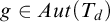 as an oracle, searches in parallel for a witness to (1), a witness to (2), and a sufficiently long piece of the axis in (3) so that the shift becomes visible. It then outputs the corresponding value of the scale.
9 Closure properties of the class of computably t.d.l.c. groups.
All computable presentations in this section will be Baire presentations (see Definition 7.1), and we will usually view a t.d.l.c. group G concretely as a computable Baire presentation. Extending the previous notation in the setting of closed subgroups of
$S_\infty $
 , by
${Tree}(G) $
, by
${Tree}(G) $
 we denote the c.l.c. tree underlying this computable Baire presentation. The following is immediate.
Fact 9.1 (Computable closed subgroups).
Let G be a computably t.d.l.c. group. Let H be a closed subgroup of G, and note that
${Tree}(H) $
 is a subtree of
${Tree}(G) $
is a subtree of
${Tree}(G) $
 . Suppose that
${Tree}(H) $
. Suppose that
${Tree}(H) $
 is computable, and hence c.l.c. Then H is computably t.d.l.c. via the Baire presentation based on
${Tree}(H) $
is computable, and hence c.l.c. Then H is computably t.d.l.c. via the Baire presentation based on
${Tree}(H) $
 , with the operations of G restricted to H.
For instance, consider the closed subgroups
$U(F)$
 of
${Aut}(T_d)$
of
${Aut}(T_d)$
 introduced by Burger and Mozes [Reference Burger and Mozes3], where
$d \ge 3$
introduced by Burger and Mozes [Reference Burger and Mozes3], where
$d \ge 3$
 and
$F $
and
$F $
 is a subgroup of
$S_d$
is a subgroup of
$S_d$
 . By Example 3.4 together with the preceding fact, each group
$U(F)$
. By Example 3.4 together with the preceding fact, each group
$U(F)$
 is computably t.d.l.c. For another example, consider the computable Baire presentation of
$\operatorname {\mathrm {SL}}_2({\mathbb {Q}}_p)$
is computably t.d.l.c. For another example, consider the computable Baire presentation of
$\operatorname {\mathrm {SL}}_2({\mathbb {Q}}_p)$
 given by Proposition 7.8. Let S be the c.l.c. subtree of T whose paths describe matrices of the form
$\begin {pmatrix} r & 0\\0 & s \end {pmatrix}$
given by Proposition 7.8. Let S be the c.l.c. subtree of T whose paths describe matrices of the form
$\begin {pmatrix} r & 0\\0 & s \end {pmatrix}$
 (so that
$s= r^{-1}$
(so that
$s= r^{-1}$
 ). This yields a computable Baire presentation of the group
$({\mathbb {Q}}_p^*, \cdot )$
). This yields a computable Baire presentation of the group
$({\mathbb {Q}}_p^*, \cdot )$
 .
.
Proposition 9.2. For each prime p and
$n \ge 2$
 , the group
$\operatorname {\mathrm {GL}}_n({\mathbb {Q}}_p)$
, the group
$\operatorname {\mathrm {GL}}_n({\mathbb {Q}}_p)$
 is computably t.d.l.c.
Proof. We employ the embedding
$F\colon GL_n({\mathbb {Q}}_p) \to SL_{n+1}({\mathbb {Q}}_p)$
 which extends a matrix A to the matrix B where the new row and new column vanish except for the diagonal element (which necessarily equals
$(\det A)^{-1}$
which extends a matrix A to the matrix B where the new row and new column vanish except for the diagonal element (which necessarily equals
$(\det A)^{-1}$
 ). Clearly there is a c.l.c. subtree S of the c.l.c. subtree of T in Proposition 7.8 for
$n+1$
). Clearly there is a c.l.c. subtree S of the c.l.c. subtree of T in Proposition 7.8 for
$n+1$
 such that
$[S] = \mathrm {range} (F)$
such that
$[S] = \mathrm {range} (F)$
 . Now we apply Fact 9.1.
A further construction staying within the class of t.d.l.c. groups is the semidirect product based on a continuous action. In the effective setting, we use actions that are computable in the sense of Section 6. For computable actions in the more general context of Polish groups, see [Reference Melnikov and Montalbán32].
Proposition 9.3 (Closure under computable semidirect products).
Let
$G, H$
 be computably t.d.l.c. groups. Suppose
$\Gamma \colon G \times H \to H $
be computably t.d.l.c. groups. Suppose
$\Gamma \colon G \times H \to H $
 is a computable function (as in Definition 6.3) that specifies an action of G on H via topological automorphisms. Then the topological semidirect product
$L=G \ltimes _\Gamma H$
is a computable function (as in Definition 6.3) that specifies an action of G on H via topological automorphisms. Then the topological semidirect product
$L=G \ltimes _\Gamma H$
 is computably t.d.l.c.
Proof. Let T be the tree obtained by interspersing strings of the same length from the trees of G and H, i.e.,

It is clear that T is a c.l.c. tree. Via the natural bijection

one can write elements of L in the form
$\langle g, h \rangle $
 where
$g\in [{Tree}(G) ]$
where
$g\in [{Tree}(G) ]$
 and
$h \in [{Tree}(H) ]$
and
$h \in [{Tree}(H) ]$
 .
.
By the standard definition of a semidirect product [Reference Robinson48, p. 27], writing the operations for G and H in the usual group theoretic way, we have

This shows that
${Mult}$
 and
${Inv}$
and
${Inv}$
 are computable, and hence yields a computable Baire presentation
$([T], {Mult}, {Inv})$
are computable, and hence yields a computable Baire presentation
$([T], {Mult}, {Inv})$
 for L.
Remark 9.4. The foregoing proposition leads to a different proof that
$\operatorname {\mathrm {GL}}_n({\mathbb {Q}}_p)$
 is computably t.d.l.c. (Proposition 9.2). To simplify notation we let
$n=2$
is computably t.d.l.c. (Proposition 9.2). To simplify notation we let
$n=2$
 ; it is not hard to generalise the argument below to a general n. As mentioned after Fact 9.1, there is a computable Baire presentation of
$({\mathbb {Q}}_p^*, \cdot )$
; it is not hard to generalise the argument below to a general n. As mentioned after Fact 9.1, there is a computable Baire presentation of
$({\mathbb {Q}}_p^*, \cdot )$
 . We have
$\operatorname {\mathrm {GL}}_2({\mathbb {Q}}_p) = {\mathbb {Q}}_p^* \ltimes _\Phi \operatorname {\mathrm {SL}}_2({\mathbb {Q}}_p)$
. We have
$\operatorname {\mathrm {GL}}_2({\mathbb {Q}}_p) = {\mathbb {Q}}_p^* \ltimes _\Phi \operatorname {\mathrm {SL}}_2({\mathbb {Q}}_p)$
 via the inclusion embedding of
$\operatorname {\mathrm {SL}}_2({\mathbb {Q}}_p)$
via the inclusion embedding of
$\operatorname {\mathrm {SL}}_2({\mathbb {Q}}_p)$
 , the embedding
$q \to \begin {pmatrix} q & 0\\0 & 1\end {pmatrix}$
, the embedding
$q \to \begin {pmatrix} q & 0\\0 & 1\end {pmatrix}$
 of
${\mathbb {Q}}_p^*$
of
${\mathbb {Q}}_p^*$
 , and the computable action
$\Phi (q, \begin {pmatrix} a & b\\c & d \end {pmatrix}) = \begin {pmatrix} a & q^{-1} b\\qc & d \end {pmatrix}$
, and the computable action
$\Phi (q, \begin {pmatrix} a & b\\c & d \end {pmatrix}) = \begin {pmatrix} a & q^{-1} b\\qc & d \end {pmatrix}$
 .
.
Note that the two computable Baire presentations of
$GL_2({\mathbb {Q}}_p)$
 obtained above are computably isomorphic: one maps
$(q, \begin {pmatrix} a & b\\c & d \end {pmatrix})$
obtained above are computably isomorphic: one maps
$(q, \begin {pmatrix} a & b\\c & d \end {pmatrix})$
 to
$\begin {pmatrix} qa & q b & 0\\c & d & 0 \\ 0 & 0 & q^{-1}\end {pmatrix}$
to
$\begin {pmatrix} qa & q b & 0\\c & d & 0 \\ 0 & 0 & q^{-1}\end {pmatrix}$
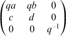 .
.
Given a sequence of t.d.l.c. groups
$(G_i) _{i\in {\mathbb {N}}^+} $
 , the direct product
$\prod _{i\in {\mathbb {N}}^+} G_i$
, the direct product
$\prod _{i\in {\mathbb {N}}^+} G_i$
 is not t.d.l.c. in general. In [Reference Wesolek56, Definition 2.3] a local direct product is described that retains the property of being t.d.l.c. This construction depends on the choices of compact open subgroups
$U_i$
is not t.d.l.c. in general. In [Reference Wesolek56, Definition 2.3] a local direct product is described that retains the property of being t.d.l.c. This construction depends on the choices of compact open subgroups
$U_i$
 of
$G_i$
of
$G_i$
 , for each i: let
$G= \bigoplus _i (G_i, U_i) $
, for each i: let
$G= \bigoplus _i (G_i, U_i) $
 consist of the elements
$f \in \prod _i G_i$
consist of the elements
$f \in \prod _i G_i$
 such that
$f(i) \in U_i$
such that
$f(i) \in U_i$
 for sufficiently large i. We have
$G = \bigcup _{k\in {\mathbb {N}}} H_k$
for sufficiently large i. We have
$G = \bigcup _{k\in {\mathbb {N}}} H_k$
 where
$H_0= \prod _{i\in {\mathbb {N}}^+} U_i$
where
$H_0= \prod _{i\in {\mathbb {N}}^+} U_i$
 and for
$k>0$
and for
$k>0$
 ,
$H_k= G_1 \times \cdots \times G_{k} \times \prod _{ i> k} U_i$
,
$H_k= G_1 \times \cdots \times G_{k} \times \prod _{ i> k} U_i$
 . The groups
$H_k$
. The groups
$H_k$
 are equipped with the product topology. A set
$W \subseteq G$
are equipped with the product topology. A set
$W \subseteq G$
 is declared open if
$W \cap H_k$
is declared open if
$W \cap H_k$
 is open for each k. (In particular,
$\prod _i U_i$
is open for each k. (In particular,
$\prod _i U_i$
 is a compact open subgroup.)
Fix a computable bijection
$\langle ., .\rangle \colon {\mathbb {N}} \times {\mathbb {N}}^+ \to {\mathbb {N}}$
 such that
$\langle a,b\rangle \ge \max (a,b)$
such that
$\langle a,b\rangle \ge \max (a,b)$
 . For a string
$\sigma \in {\mathbb {N}}^*$
. For a string
$\sigma \in {\mathbb {N}}^*$
 and
$i>0$
and
$i>0$
 , by
$\sigma ^{(i)}$
, by
$\sigma ^{(i)}$
 we denote the string
$\tau $
we denote the string
$\tau $
 of maximum length such that
$\tau (k)= \sigma (\langle k, i\rangle )$
of maximum length such that
$\tau (k)= \sigma (\langle k, i\rangle )$
 for each
$k < |\tau |$
for each
$k < |\tau |$
 . Similarly, for
$f \colon {\mathbb {N}} \to {\mathbb {N}}$
. Similarly, for
$f \colon {\mathbb {N}} \to {\mathbb {N}}$
 we define
$f^{(i)}$
we define
$f^{(i)}$
 to be the function such that
$f^{(i)}(k)= f(\langle k, i\rangle ) $
to be the function such that
$f^{(i)}(k)= f(\langle k, i\rangle ) $
 for each k. Given uniformly computable subtrees
$B_i$
for each k. Given uniformly computable subtrees
$B_i$
 of
${\mathbb {N}}^*$
of
${\mathbb {N}}^*$
 , by
$B=\prod _i B_i$
, by
$B=\prod _i B_i$
 we denote the computable tree
$\{ \sigma \colon \forall i [ \sigma ^{(i)} \in B_i]\}$
we denote the computable tree
$\{ \sigma \colon \forall i [ \sigma ^{(i)} \in B_i]\}$
 . Note that
$[B]$
. Note that
$[B]$
 is canonically homeomorphic to
$\prod _i [B_i]$
is canonically homeomorphic to
$\prod _i [B_i]$
 via
$f \to (f^{(i)})_{i\in {\mathbb {N}}}$
via
$f \to (f^{(i)})_{i\in {\mathbb {N}}}$
 . So we can specify a path f of B by specifying all the
$f^{(i)}$
. So we can specify a path f of B by specifying all the
$f^{(i)}$
 .
.
Proposition 9.5 (Local direct products).
Let
$(G_i)_{i\in {\mathbb {N}}^+}$
 be computable Baire presentations
$(T_i, {Mult}_i, {Inv}_i)$
be computable Baire presentations
$(T_i, {Mult}_i, {Inv}_i)$
 uniformly in i, and suppose that there is
$k \in {\mathbb {N}}^+$
uniformly in i, and suppose that there is
$k \in {\mathbb {N}}^+$
 such that each
$T_i$
such that each
$T_i$
 is c.l.c. via k. Suppose further that
$U_i$
is c.l.c. via k. Suppose further that
$U_i$
 is a compact open subgroup of
$G_i$
is a compact open subgroup of
$G_i$
 , uniformly in i. Then
$G=\bigoplus _{i\in {\mathbb {N}}^+} (G_i, U_i) $
, uniformly in i. Then
$G=\bigoplus _{i\in {\mathbb {N}}^+} (G_i, U_i) $
 is computably t.d.l.c.
Proof. The uniformity hypothesis on the
$U_i$
 means that there is a computable function q such that
$\mathcal {K}_{q(i)}^{T_i}= U_i$
means that there is a computable function q such that
$\mathcal {K}_{q(i)}^{T_i}= U_i$
 . We use these data to build a computable Baire presentation
$([T], {Mult}, {Inv})$
. We use these data to build a computable Baire presentation
$([T], {Mult}, {Inv})$
 of G. We aim at defining uniformly c.l.c. trees
$V_r$
of G. We aim at defining uniformly c.l.c. trees
$V_r$
 such that as topological spaces,
$[V_0]$
such that as topological spaces,
$[V_0]$
 is homeomorphic to
$H_0$
is homeomorphic to
$H_0$
 defined above, and for
$r>0$
defined above, and for
$r>0$
 ,
$V_r$
,
$V_r$
 is homeomorphic to
$H_r - H_{r-1}$
is homeomorphic to
$H_r - H_{r-1}$
 . All these homeomorphisms are canonically given, as can be seen during the construction of the
$V_r$
. All these homeomorphisms are canonically given, as can be seen during the construction of the
$V_r$
 . Our Baire presentation of G will be based on the c.l.c. tree

It is easy to verify that
$[T]$
 is homeomorphic to G, using that the
$H_r$
is homeomorphic to G, using that the
$H_r$
 are open subgroups of G.
Towards defining the trees
$V_r$
 , let
$R_i$
, let
$R_i$
 be the subtree of
$T_i$
be the subtree of
$T_i$
 without leaves such that
$[R_i]= U_i$
without leaves such that
$[R_i]= U_i$
 , and let
$S_i$
, and let
$S_i$
 be the subtree of
$T_i$
be the subtree of
$T_i$
 such that
$[S_i]= [T_i]-U_i$
such that
$[S_i]= [T_i]-U_i$
 .
.
Claim 9.6. The trees
$R_i, S_i$
 are c.l.c. trees uniformly in
$i \in {\mathbb {N}}^+$
are c.l.c. trees uniformly in
$i \in {\mathbb {N}}^+$
 .
.
To check this, it suffices to show that these trees are uniformly computable. Given i, let
$F_i \subseteq {\mathbb {N}}^*$
 be the finite set with strong index
$q(i)$
be the finite set with strong index
$q(i)$
 . Note that
$R_i$
. Note that
$R_i$
 consists of the strings compatible with a string in
$F_i$
consists of the strings compatible with a string in
$F_i$
 , which is a decidable condition uniformly in i. To determine whether
$\tau \in S_i$
, which is a decidable condition uniformly in i. To determine whether
$\tau \in S_i$
 ,
,
-
(i) First check whether some prefix of $\tau $
is in F; if so, answer “no.” -
(ii) Otherwise, using the conditions defining c.l.c. trees check whether $[\tau ]_{T_i}$
is compact; if not answer “yes.” If so, check whether
$\tau $
has an extension longer that any string in
$F_i$
that is not in
$R_i$
; if so answer “yes,” otherwise “no.”


This shows the claim.
Now let
$V_0= \prod _i R_i$
 , and for
$r>0$
, and for
$r>0$
 let
let

interpreted as subtrees of
$\prod _i T_i$
 in the obvious way. (So, f is a path of
$V_r$
in the obvious way. (So, f is a path of
$V_r$
 iff
$f^{(i)}$
iff
$f^{(i)}$
 is a path of
$T_i$
is a path of
$T_i$
 for
$1\le i<r$
for
$1\le i<r$
 ,
$f^{(r)}$
,
$f^{(r)}$
 is not in
$U_{r}$
is not in
$U_{r}$
 , but
$f^{(i)}$
, but
$f^{(i)}$
 is in
$U_i$
is in
$U_i$
 for
$i>r$
for
$i>r$
 .) It is easy to check that the trees
$V_r$
.) It is easy to check that the trees
$V_r$
 are uniformly c.l.c.
Uniformly in r, on
$[V_r]$
 we have a computable function
$L_r$
we have a computable function
$L_r$
 given by
$L_r(f)^{(i)}= {Inv}_i(f^{(i)})$
given by
$L_r(f)^{(i)}= {Inv}_i(f^{(i)})$
 . So there is a computable function
${Inv}$
. So there is a computable function
${Inv}$
 on
$[T]$
on
$[T]$
 given by

Next, for
$r,s \in {\mathbb {N}}$
 and
$rf, sg \in [T]$
and
$rf, sg \in [T]$
 , let
, let

where h is the function given by
$h^{(i)} = {Mult}_i(f^{(i)}, g^{(i)})$
 , and
$t \le \max (r,s)$
, and
$t \le \max (r,s)$
 is the least number such that
$t=0$
is the least number such that
$t=0$
 , or
$t>0$
, or
$t>0$
 and
$h^{(t)}\! \upharpoonright _{ \max (F_{t})}\in S_{t}$
and
$h^{(t)}\! \upharpoonright _{ \max (F_{t})}\in S_{t}$
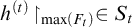 . That is, we compute the binary group operation componentwise, and then check which tree
$V_t$
. That is, we compute the binary group operation componentwise, and then check which tree
$V_t$
 the overall result is a path of; this can be done because from
$\max (r,s)$
the overall result is a path of; this can be done because from
$\max (r,s)$
 on, the component of the result will be in the relevant compact open subgroup.
It should be clear that, via the homeomorphism of the spaces
$[T]$
 and G outlined above,
$([T], {Mult}, {Inv})$
and G outlined above,
$([T], {Mult}, {Inv})$
 is a computable Baire presentation of G.
We note that the hypothesis that
$T_i$
 is c.l.c. via a fixed k is one of notational convenience; what matters is that given i we can compute
$\ell _i$
is c.l.c. via a fixed k is one of notational convenience; what matters is that given i we can compute
$\ell _i$
 such that
$T_i$
such that
$T_i$
 is c.l.c. via
$\ell _i$
is c.l.c. via
$\ell _i$
 . This is so because, given a tree T that is c.l.c. via
$\ell $
. This is so because, given a tree T that is c.l.c. via
$\ell $
 , we can uniformly transform it into an equivalent tree
$\widetilde T$
, we can uniformly transform it into an equivalent tree
$\widetilde T$
 that is c.l.c. via
$1$
that is c.l.c. via
$1$
 , by “skipping” the levels
$1, \dots , \ell -1$
, by “skipping” the levels
$1, \dots , \ell -1$
 .
.
The hardest result in this section will be tackled last: being computably t.d.l.c. is preserved under taking quotients by computable normal closed subgroups. As an application we will show that the groups
$PGL_n({\mathbb {Q}}_p)$
 are computably t.d.l.c. For
$n=2$
are computably t.d.l.c. For
$n=2$
 these groups have been the subject of much research; for instance, they are homeomorphic to closed subgroups of
${Aut} (T_{p+1})$
these groups have been the subject of much research; for instance, they are homeomorphic to closed subgroups of
${Aut} (T_{p+1})$
 as shown by Serre [Reference Serre51, Section II.1].
First we need some notation and preliminaries. The variables
$\alpha , \beta ,$
 etc. will range over strings in
${\mathbb {N}}^*$
etc. will range over strings in
${\mathbb {N}}^*$
 without repetitions. The variables
$P, Q, R $
without repetitions. The variables
$P, Q, R $
 range over permutations of
${\mathbb {N}}$
range over permutations of
${\mathbb {N}}$
 . Recall from Section 3.1 that in our setup the elements of
$S_\infty $
. Recall from Section 3.1 that in our setup the elements of
$S_\infty $
 have the form
$P\oplus P^{-1}$
have the form
$P\oplus P^{-1}$
 where P is a permutation of
${\mathbb {N}}$
where P is a permutation of
${\mathbb {N}}$
 . It appears that a crucial “finitization” argument, Claim 9.11, is best shown in the setting of true permutations, rather than elements of
$S_\infty $
. It appears that a crucial “finitization” argument, Claim 9.11, is best shown in the setting of true permutations, rather than elements of
$S_\infty $
 in our setup. So we need two lemmas allowing us to pass back and forth between the two.
We adopt the setting of Theorem 8.2: let
$G=([T], {Mult}, {Inv}) $
 be a computable Baire presentation, let
$\mathcal {W}$
be a computable Baire presentation, let
$\mathcal {W}$
 be a Haar computable copy of
$\mathcal {W}(G)$
be a Haar computable copy of
$\mathcal {W}(G)$
 with domain
${\mathbb {N}}$
with domain
${\mathbb {N}}$
 , and let
$\widetilde G$
, and let
$\widetilde G$
 be as detailed there; in particular,
$S= {Tree}(\widetilde G) $
be as detailed there; in particular,
$S= {Tree}(\widetilde G) $
 is c.l.c. via
$k=2$
is c.l.c. via
$k=2$
 , so that
$[\sigma ]_S$
, so that
$[\sigma ]_S$
 is compact for each string
$\sigma $
is compact for each string
$\sigma $
 of length
$\ge 2$
of length
$\ge 2$
 . Let
. Let

The first lemma verifies that
$S_0$
 is computable, and shows that from a nonempty string in
$S_0$
is computable, and shows that from a nonempty string in
$S_0$
 one can compute the set of elements of
$[S]$
one can compute the set of elements of
$[S]$
 with first component extending it.
Lemma 9.7. (i)
$S_0$
 is a computable tree.
(ii) There is a computable function
$B\colon S_0 - \{\emptyset \} \to {\mathbb {N}}$
 such that

Proof. (i) We first show that there is a computable bound
$H(k)$
 on
$\beta (k)$
on
$\beta (k)$
 that is uniformly obtained from
$\alpha $
that is uniformly obtained from
$\alpha $
 . Since
$\alpha $
. Since
$\alpha $
 is nonempty, we have
$\alpha (A)= B$
is nonempty, we have
$\alpha (A)= B$
 for some
$A,B \in \mathcal {W}$
for some
$A,B \in \mathcal {W}$
 . Hence
$f(AA^{-1})= BA^{-1}$
. Hence
$f(AA^{-1})= BA^{-1}$
 for any
$f \in \widetilde G$
for any
$f \in \widetilde G$
 such that
$\alpha \prec f$
such that
$\alpha \prec f$
 . By Lemma 5.5 with
$U= AA^{-1} $
. By Lemma 5.5 with
$U= AA^{-1} $
 ,
$L = BA^{-1}$
,
$L = BA^{-1}$
 , and F the coset denoted by k, we obtain a bound
$H(k)$
, and F the coset denoted by k, we obtain a bound
$H(k)$
 as required. This shows that from
$\alpha $
as required. This shows that from
$\alpha $
 one can compute a finite set of possible candidates for
$\beta $
one can compute a finite set of possible candidates for
$\beta $
 . So
$S_0$
. So
$S_0$
 is computable.
(ii) Given a nonempty
$\alpha \in S_0$
 , by the argument above we can compute a strong index
$B(\alpha ) $
, by the argument above we can compute a strong index
$B(\alpha ) $
 for the set of strings of the form
$ \alpha \oplus \beta $
for the set of strings of the form
$ \alpha \oplus \beta $
 in S.
in S.
The second lemma takes a string in
$S^{[\ge 2]}$
 and writes the paths of S extending it in terms of a finite set of strings in
$S_0$
and writes the paths of S extending it in terms of a finite set of strings in
$S_0$
 .
.
Lemma 9.8. Given
$\sigma \in S$
 such that
$|\sigma | \ge 2$
such that
$|\sigma | \ge 2$
 , one can compute (a strong index for) a finite set
$F \subseteq S_0$
, one can compute (a strong index for) a finite set
$F \subseteq S_0$
 such that

Proof. Let
$n = \max (\sigma )+1$
 . Let F consist of the strings
$\alpha \in S_0$
. Let F consist of the strings
$\alpha \in S_0$
 of length n such that viewed as an injection,
$\alpha $
of length n such that viewed as an injection,
$\alpha $
 extends the injection
$\alpha _\sigma $
extends the injection
$\alpha _\sigma $
 associated with
$\sigma $
associated with
$\sigma $
 as in (1). Since
$|\sigma | \ge 2$
as in (1). Since
$|\sigma | \ge 2$
 , by Lemma 5.5 we can compute a strong index for F. If
$\alpha \in F$
, by Lemma 5.5 we can compute a strong index for F. If
$\alpha \in F$
 and
$P \succ \alpha $
and
$P \succ \alpha $
 , then
$P \oplus P^{-1} \in [\sigma ]_S$
, then
$P \oplus P^{-1} \in [\sigma ]_S$
 , because P extends
$\alpha _\sigma $
, because P extends
$\alpha _\sigma $
 . Conversely, if
$P \oplus P^{-1} \in [\sigma ]_S$
. Conversely, if
$P \oplus P^{-1} \in [\sigma ]_S$
 , then
$P \! \upharpoonright _{n} \in F$
, then
$P \! \upharpoonright _{n} \in F$
 .
.
Theorem 9.9. Let G be computably t.d.l.c. Let N be a closed normal subgroup of G such that
${Tree}(N) $
 is a computable subtree of
${Tree}(G) $
is a computable subtree of
${Tree}(G) $
 . Then
$G/N$
. Then
$G/N$
 is computably t.d.l.c.
Proof. We continue to adopt the setting of Theorem 8.2. Recall that
$S = {Tree}( \widetilde G) $
 , and
$S_0= \{\emptyset \} \cup \{ \alpha \colon \, \exists \beta [ |\alpha | = |\beta |> 0 \, \land \, \alpha \oplus \beta \in S\}$
, and
$S_0= \{\emptyset \} \cup \{ \alpha \colon \, \exists \beta [ |\alpha | = |\beta |> 0 \, \land \, \alpha \oplus \beta \in S\}$
 . Let
$M= \Phi (N)$
. Let
$M= \Phi (N)$
 where
$\Phi $
where
$\Phi $
 is the bicomputable homeomorphism
$G \to \widetilde G$
is the bicomputable homeomorphism
$G \to \widetilde G$
 established in Theorem 8.2. Note that
${Tree}(M) $
established in Theorem 8.2. Note that
${Tree}(M) $
 is a computable subtree of S; given
$\tau \in S$
is a computable subtree of S; given
$\tau \in S$
 , one can search for a string
$\sigma \in {Tree}(G) $
, one can search for a string
$\sigma \in {Tree}(G) $
 such that
$P_\Phi (\sigma ) \succeq \tau $
such that
$P_\Phi (\sigma ) \succeq \tau $
 ; then
$\tau \in {Tree}(M) $
; then
$\tau \in {Tree}(M) $
 iff
$\sigma \in {Tree}(N) $
iff
$\sigma \in {Tree}(N) $
 .
.
We will build a Haar computable copy
$\mathcal {V}$
 of
$\mathcal {W}(\widetilde G/M)$
of
$\mathcal {W}(\widetilde G/M)$
 . We use that each compact open subset of
$\widetilde G/M$
. We use that each compact open subset of
$\widetilde G/M$
 has the form
$M \mathcal {K}$
has the form
$M \mathcal {K}$
 where
$\mathcal {K}$
where
$\mathcal {K}$
 is a compact open subset of
$\widetilde G$
is a compact open subset of
$\widetilde G$
 . In the first step, we will show that the pre-ordering “
$\mathcal {K} \subseteq M \mathcal {L}$
. In the first step, we will show that the pre-ordering “
$\mathcal {K} \subseteq M \mathcal {L}$
 ” is decidable, where
$\mathcal {K}, \mathcal {L}$
” is decidable, where
$\mathcal {K}, \mathcal {L}$
 range over compact open sets. In the second step, we will use as the domain of
$\mathcal {V}$
range over compact open sets. In the second step, we will use as the domain of
$\mathcal {V}$
 the least numbers in the classes of the computable equivalence relation associated with this pre-ordering.
We may assume that
$\mathcal {K}= [\sigma ]_S$
 for some string
$\sigma \in S$
for some string
$\sigma \in S$
 of length at least
$2$
of length at least
$2$
 . So the following suffices for the first step.
Lemma 9.10. Given strings
$\sigma , \tau _1, \ldots , \tau _r \in S$
 of length at least
$2$
of length at least
$2$
 , one can decide whether the inclusion
$[\sigma ]_S \subseteq \bigcup _i M [\tau _i]_S$
, one can decide whether the inclusion
$[\sigma ]_S \subseteq \bigcup _i M [\tau _i]_S$
 holds.
To verify the lemma, let
$ M_0 = \{ P \colon P \oplus P^{-1} \in M\}$
 . For each
$\alpha \in S_0$
. For each
$\alpha \in S_0$
 , let
, let

Recall here that P is a permutation of
$ {\mathbb {N}}$
 , not merely a path of
$S_0$
, not merely a path of
$S_0$
 (which in general could fail to be onto). Let

By Lemma 9.8, it is sufficient to decide whether a version of the inclusion holds that only refers to the permutations, not directly to their inverses.
Claim 9.11. For
$\alpha , \beta _1, \ldots , \beta _k \in S_0$
 one can decide whether
$ \underline \alpha \subseteq \bigcup _i M_0 \underline {\beta _i}$
one can decide whether
$ \underline \alpha \subseteq \bigcup _i M_0 \underline {\beta _i}$
 .
.
We may assume that
$|\alpha | \ge m:= 1+ \max _i \max (\beta _i)$
 . We show that m is the maximum height on
$T_0$
. We show that m is the maximum height on
$T_0$
 relevant for this inclusion: for each i,

For the implication “
$\Rightarrow $
 ”, simply let
$\eta = Q \! \upharpoonright _{m}$
”, simply let
$\eta = Q \! \upharpoonright _{m}$
 . For the implication “
$\Leftarrow $
. For the implication “
$\Leftarrow $
 ”, fix a permutation
$Q \succ \eta $
”, fix a permutation
$Q \succ \eta $
 such that
$Q \in M_0$
such that
$Q \in M_0$
 . Given
$P \in \underline \alpha $
. Given
$P \in \underline \alpha $
 , we can choose
$R \in \underline \eta $
, we can choose
$R \in \underline \eta $
 and
$R' \in \underline {\beta _i}$
and
$R' \in \underline {\beta _i}$
 such that
$P= R \circ R'$
such that
$P= R \circ R'$
 . Since
$R, Q \succ \eta $
. Since
$R, Q \succ \eta $
 and
$|\eta |= m> \max (\beta _i)$
and
$|\eta |= m> \max (\beta _i)$
 , we have
$Q^{-1} \circ R \circ R' \succ \beta _i$
, we have
$Q^{-1} \circ R \circ R' \succ \beta _i$
 . So
$P \in M_0 \circ \underline {\beta _i}$
. So
$P \in M_0 \circ \underline {\beta _i}$
 via Q. This verifies the equivalence (3).
Using (3), if
$ \underline \alpha \subseteq \bigcup _i M_0 \circ \underline {\beta _i}$
 , then because
$|\alpha |> \max _i |\beta _i|$
, then because
$|\alpha |> \max _i |\beta _i|$
 , we have
$\underline \alpha \subseteq M_0 \circ \underline \beta _i$
, we have
$\underline \alpha \subseteq M_0 \circ \underline \beta _i$
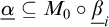 for some single i. If
$\eta $
for some single i. If
$\eta $
 works on the right hand side of (3) then
$\eta (\beta _i(0))= \alpha (0)$
works on the right hand side of (3) then
$\eta (\beta _i(0))= \alpha (0)$
 . So by Lemma 5.5 again, there is a computable bound
$H(k)$
. So by Lemma 5.5 again, there is a computable bound
$H(k)$
 on
$\eta (k)$
on
$\eta (k)$
 that is uniformly obtained from the values
$\alpha (0), \beta _1(0), \ldots , \beta _k(0)$
that is uniformly obtained from the values
$\alpha (0), \beta _1(0), \ldots , \beta _k(0)$
 . This shows that one can compute a strong index for a finite set containing all potential witnesses
$\eta $
. This shows that one can compute a strong index for a finite set containing all potential witnesses
$\eta $
 on the right hand side of (3). For each such
$\eta $
on the right hand side of (3). For each such
$\eta $
 , using Lemma 9.7(ii), it is equivalent to decide whether
$\mathcal {K}_{B(\alpha )} \subseteq \mathcal {K}_{B(\eta )} \mathcal {K}_{B( \beta _i)}$
, using Lemma 9.7(ii), it is equivalent to decide whether
$\mathcal {K}_{B(\alpha )} \subseteq \mathcal {K}_{B(\eta )} \mathcal {K}_{B( \beta _i)}$
 , which can be done using Lemma 7.5(ii). This shows the claim and hence verifies Lemma 9.10.
By the lemma (and the discussion preceding it), the equivalence relation on
${\mathbb {N}}$
 given by

is computable; recall here that
$\mathcal {W}$
 has domain
${\mathbb {N}}$
has domain
${\mathbb {N}}$
 . As the domain
$\mathcal {D}$
. As the domain
$\mathcal {D}$
 of the computable copy
$\mathcal {V}$
of the computable copy
$\mathcal {V}$
 of
$\mathcal {W}(\widetilde G/M)$
of
$\mathcal {W}(\widetilde G/M)$
 , we use the computable set of least elements of equivalence classes.
We think of an element A of
$\mathcal {D}$
 as denoting the compact open coset
$A M$
as denoting the compact open coset
$A M$
 of
$\widetilde G/ M$
of
$\widetilde G/ M$
 . Given
$A,B \in \mathcal {W} $
. Given
$A,B \in \mathcal {W} $
 we have
$(A M)^{-1} = A^{-1} M$
we have
$(A M)^{-1} = A^{-1} M$
 and
$(AM ) (B M)= (AB) M$
and
$(AM ) (B M)= (AB) M$
 . In particular, one can decide whether
$A M $
. In particular, one can decide whether
$A M $
 , viewed as a subset of
$\widetilde G/M$
, viewed as a subset of
$\widetilde G/M$
 , is a left coset of a subgroup of
$\widetilde G/ M$
, is a left coset of a subgroup of
$\widetilde G/ M$
 that
$B M$
that
$B M$
 is a right coset of. So by Lemma 3.5 the groupoid operations are computable on D.
For the computability of the meet operation, suppose
$A,B \in \mathcal {W}$
 are given. One has
$AN \cap BN = (A \cap BN) N$
are given. One has
$AN \cap BN = (A \cap BN) N$
 . Suppose
$A $
. Suppose
$A $
 is a left coset of the subgroup U and B is a left coset of the subgroup V. Then
$A \cap BN$
is a left coset of the subgroup U and B is a left coset of the subgroup V. Then
$A \cap BN$
 is a left coset of the compact open subgroup
$U \cap VN$
is a left coset of the compact open subgroup
$U \cap VN$
 . Note that

(The inclusion
$\supseteq $
 is trivial. For
$\subseteq $
is trivial. For
$\subseteq $
 , if
$x \in A \cap BN$
, if
$x \in A \cap BN$
 , then
$ x \in L$
, then
$ x \in L$
 for some left coset of
$U \cap V$
for some left coset of
$U \cap V$
 . Since
$x = bn$
. Since
$x = bn$
 for some
$b\in B, n \in M$
for some
$b\in B, n \in M$
 we have
$LN = BN$
we have
$LN = BN$
 .) So one can compute
$C \in \mathcal {W}$
.) So one can compute
$C \in \mathcal {W}$
 such that
$C= A \cap BN$
such that
$C= A \cap BN$
 using Lemma 2.6. Then one outputs the element
$C'$
using Lemma 2.6. Then one outputs the element
$C'$
 of
$\mathcal {D}$
of
$\mathcal {D}$
 such that
$C' \sim C$
such that
$C' \sim C$
 .
.
Finally, to show that
$\mathcal {V}$
 is Haar computable, note that
$|UN : UN \cap VN|= |U \colon U \cap VN|$
is Haar computable, note that
$|UN : UN \cap VN|= |U \colon U \cap VN|$
 . By the above (in the special case that A and B are subgroups) one can compute
$U \cap VN \in \mathcal {W}$
. By the above (in the special case that A and B are subgroups) one can compute
$U \cap VN \in \mathcal {W}$
 . So one can compute the index using that
$\mathcal {W}$
. So one can compute the index using that
$\mathcal {W}$
 is Haar computable.
Example 9.12. For each prime p and each
$n \ge 2$
 , the group
$\operatorname {\mathrm {PGL}}_n({\mathbb {Q}}_p)$
, the group
$\operatorname {\mathrm {PGL}}_n({\mathbb {Q}}_p)$
 is computably t.d.l.c.
Proof. We use the computable Baire presentation
$(T, {Mult}, {Inv}) $
 of
$\operatorname {\mathrm {GL}}_n({\mathbb {Q}}_p)$
of
$\operatorname {\mathrm {GL}}_n({\mathbb {Q}}_p)$
 obtained in Proposition9.2. In this presentation, the centre N of
$\operatorname {\mathrm {GL}}_n({\mathbb {Q}}_p)$
obtained in Proposition9.2. In this presentation, the centre N of
$\operatorname {\mathrm {GL}}_n({\mathbb {Q}}_p)$
 is given by the diagonal
$(n+1) \times (n+1)$
is given by the diagonal
$(n+1) \times (n+1)$
 matrices such that the first n entries of the diagonal agree. So clearly
${Tree}(N) $
matrices such that the first n entries of the diagonal agree. So clearly
${Tree}(N) $
 is a computable sub-tree of the tree S in Proposition 9.2. Hence we can apply Theorem 9.9.
10 Uniqueness of computable presentations.
As discussed in Section 1.8, in computable structure theory a countable structure is called autostable, or computably categorical, if it has a computable copy, and all its computable copies are computably isomorphic. We adapt this notion to the present setting.
Definition 10.1. A computably t.d.l.c. group G is called autostable if for any two computable Baire presentations of G, based on trees
$T, S\subseteq {\mathbb {N}}^*$
 , there is a computable group homeomorphism
$\Psi \colon [T] \to [S]$
, there is a computable group homeomorphism
$\Psi \colon [T] \to [S]$
 .
.
Note that
$\Psi ^{-1}$
 is also computable by Corollary 8.3. For abelian profinite groups, the notion of autostability used in [Reference Melnikov31] is equivalent to our definition. This follows from the proofs of Propositions B.6 and B.7, which show that in the abelian case the correspondence between Baire presentations and procountable presentations is uniform and witnessed by uniformly obtained group isomorphisms between these presentations. The first author [Reference Melnikov31, Corollary 1.11] characterized autostability for abelian compact pro-p groups given by computable procountable presentations with effectively finite kernels: such a group is autostable iff its Pontryagin–van Kampen dual is autostable. For instance,
$({\mathbb {Z}}_p, +)$
is also computable by Corollary 8.3. For abelian profinite groups, the notion of autostability used in [Reference Melnikov31] is equivalent to our definition. This follows from the proofs of Propositions B.6 and B.7, which show that in the abelian case the correspondence between Baire presentations and procountable presentations is uniform and witnessed by uniformly obtained group isomorphisms between these presentations. The first author [Reference Melnikov31, Corollary 1.11] characterized autostability for abelian compact pro-p groups given by computable procountable presentations with effectively finite kernels: such a group is autostable iff its Pontryagin–van Kampen dual is autostable. For instance,
$({\mathbb {Z}}_p, +)$
 is autostable because its dual is the Prüfer group
$C_{p^\infty }$
is autostable because its dual is the Prüfer group
$C_{p^\infty }$
 , which is easily seen to be autostable as a countable structure (see the proof of Theorem 10.6 below).
We provide a criterion for autostability, and evidence its usefulness through various examples.
Criterion 10.2. A computably t.d.l.c. group G is autostable
$\Leftrightarrow $
 any two Haar computable copies of its meet groupoid
$\mathcal {W}(G)$
any two Haar computable copies of its meet groupoid
$\mathcal {W}(G)$
 are computably isomorphic.
We will only apply the implication “
$\Leftarrow $
 ”. However, the converse implication is interesting on its own right because it shows that our notion of autostability is independent of whether we use computable Baire presentation, or computable presentations based on meet groupoids. In fact, the proof of the converse implication shows that we could also use presentations based on closed subgroups of
$S_\infty $
”. However, the converse implication is interesting on its own right because it shows that our notion of autostability is independent of whether we use computable Baire presentation, or computable presentations based on meet groupoids. In fact, the proof of the converse implication shows that we could also use presentations based on closed subgroups of
$S_\infty $
 .
.
Proof. We may assume that G itself is a computable Baire presentation. As before, let
$\mathcal {W} = \mathcal {W}_{\text {comp}}(G)$
 as in Notation 7.7, and let
$\widetilde G= \mathcal {G}_{\text {comp}} (\mathcal {W})$
as in Notation 7.7, and let
$\widetilde G= \mathcal {G}_{\text {comp}} (\mathcal {W})$
 as in Definition 5.2. Let
$\Phi \colon G \to \widetilde G$
as in Definition 5.2. Let
$\Phi \colon G \to \widetilde G$
 be the group homeomorphism given by Theorem 8.2.
“
$\Leftarrow $
 ”: Let
$H $
”: Let
$H $
 be a computable Baire presentation such that
$G \cong H$
be a computable Baire presentation such that
$G \cong H$
 . Let
$ \mathcal {V}= \mathcal {W}_{\text {comp}}(H)$
. Let
$ \mathcal {V}= \mathcal {W}_{\text {comp}}(H)$
 , and let
$ \widetilde H = \mathcal {G}_{\text {comp}} (\mathcal {V})$
, and let
$ \widetilde H = \mathcal {G}_{\text {comp}} (\mathcal {V})$
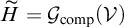 . Clearly
$G \cong H$
. Clearly
$G \cong H$
 implies
$\mathcal {W} \cong \mathcal {V}$
implies
$\mathcal {W} \cong \mathcal {V}$
 . Since
$\mathcal {V}$
. Since
$\mathcal {V}$
 is Haar computable, by hypothesis there is a computable isomorphism
$\theta \colon \mathcal {W} \to \mathcal {V}$
is Haar computable, by hypothesis there is a computable isomorphism
$\theta \colon \mathcal {W} \to \mathcal {V}$
 ; note that
$\theta $
; note that
$\theta $
 is a permutation of
${\mathbb {N}}$
is a permutation of
${\mathbb {N}}$
 , so
$\theta ^{-1}$
, so
$\theta ^{-1}$
 is also computable. We define a computable homeomorphism
$\widetilde \theta \colon \widetilde G \to \widetilde H$
is also computable. We define a computable homeomorphism
$\widetilde \theta \colon \widetilde G \to \widetilde H$
 as follows. Given
$p= f\oplus f^{-1} \in \widetilde G$
as follows. Given
$p= f\oplus f^{-1} \in \widetilde G$
 , let
, let

Using that
$\theta $
 is an isomorphism of meet groupoids, it is easy to verify that
$\widetilde \theta $
is an isomorphism of meet groupoids, it is easy to verify that
$\widetilde \theta $
 is a homeomorphism. Clearly
$\widetilde \theta $
is a homeomorphism. Clearly
$\widetilde \theta $
 is computable. The inverse of
$\widetilde \theta $
is computable. The inverse of
$\widetilde \theta $
 is given by exchanging
$\theta $
is given by exchanging
$\theta $
 and
$\theta ^{-1}$
and
$\theta ^{-1}$
 in the above, and hence is computable as well.
Let
$\Psi \colon H \to \widetilde H$
 be the homeomorphisms given by Theorem 8.2 with H in place of G. We have a group homeomorphism
$ \Psi ^{-1} \circ \widetilde \theta \circ \Phi \colon G \to H$
be the homeomorphisms given by Theorem 8.2 with H in place of G. We have a group homeomorphism
$ \Psi ^{-1} \circ \widetilde \theta \circ \Phi \colon G \to H$
 , which is computable as a composition of computable maps. Also, its inverse is computable because the inverse of
$\widetilde \theta $
, which is computable as a composition of computable maps. Also, its inverse is computable because the inverse of
$\widetilde \theta $
 is computable.
“
$\Rightarrow $
 ”: Suppose
$\mathcal {V}$
”: Suppose
$\mathcal {V}$
 is a Haar computable meet groupoid such that
$\mathcal {W} \cong \mathcal {V}$
is a Haar computable meet groupoid such that
$\mathcal {W} \cong \mathcal {V}$
 via an isomorphism
$\beta $
via an isomorphism
$\beta $
 . We need to show that
$\mathcal {W}$
. We need to show that
$\mathcal {W}$
 and
$ \mathcal {V}$
and
$ \mathcal {V}$
 are computably isomorphic. To this end, let
$\widetilde H = \mathcal {G}_{\text {comp}} (\mathcal {V})$
are computably isomorphic. To this end, let
$\widetilde H = \mathcal {G}_{\text {comp}} (\mathcal {V})$
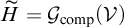 , which is a computable Baire presentation of a t.d.l.c. group (Claim 5.6). Let
$\widetilde {\mathcal {W}} = \mathcal {W}_{\text {comp}}(\widetilde G)$
, which is a computable Baire presentation of a t.d.l.c. group (Claim 5.6). Let
$\widetilde {\mathcal {W}} = \mathcal {W}_{\text {comp}}(\widetilde G)$
 and
$\widetilde {\mathcal {V}} = \mathcal {W}_{\text {comp}}(\widetilde H)$
and
$\widetilde {\mathcal {V}} = \mathcal {W}_{\text {comp}}(\widetilde H)$
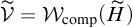 . Let
$\alpha _{\mathcal {W}} \colon \mathcal {W} \to \widetilde {\mathcal {W}}$
. Let
$\alpha _{\mathcal {W}} \colon \mathcal {W} \to \widetilde {\mathcal {W}}$
 and
$\alpha _{\mathcal {V}} \colon \mathcal {V} \to \widetilde {\mathcal {V}}$
and
$\alpha _{\mathcal {V}} \colon \mathcal {V} \to \widetilde {\mathcal {V}}$
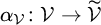 be the maps given by

where the notation
$A_U$
 indicates that
$A $
indicates that
$A $
 is a left coset of U, and as usual
$p = p_0 \oplus p_1$
is a left coset of U, and as usual
$p = p_0 \oplus p_1$
 , etc. Informally,
$\widetilde {\mathcal {W}}$
, etc. Informally,
$\widetilde {\mathcal {W}}$
 is the double dual of
$\mathcal {W}$
is the double dual of
$\mathcal {W}$
 , and
$\alpha _{\mathcal {W}}$
, and
$\alpha _{\mathcal {W}}$
 maps
$\mathcal {W}$
maps
$\mathcal {W}$
 into its double dual; a similar statement holds for
$\widetilde {\mathcal {V}}$
into its double dual; a similar statement holds for
$\widetilde {\mathcal {V}}$
 ,
$\mathcal {V,}$
,
$\mathcal {V,}$
 and
$\alpha _{\mathcal {V}}$
and
$\alpha _{\mathcal {V}}$
 . An argument similar to the one in the proof of Lemma 9.7(ii) shows that the maps
$\alpha _{\mathcal {W}}$
. An argument similar to the one in the proof of Lemma 9.7(ii) shows that the maps
$\alpha _{\mathcal {W}}$
 and
$\alpha _{\mathcal {V}}$
and
$\alpha _{\mathcal {V}}$
 are computable.
Since
$\Phi \colon G \to \widetilde G$
 is a group homeomorphism, its dual
$\widetilde \Phi \colon \mathcal {W} \to \widetilde {\mathcal {W}}$
is a group homeomorphism, its dual
$\widetilde \Phi \colon \mathcal {W} \to \widetilde {\mathcal {W}}$
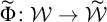 is a meet groupoid isomorphism, where
$\widetilde \Phi (A) = \{\Phi (g) \colon \, g \in A\}$
is a meet groupoid isomorphism, where
$\widetilde \Phi (A) = \{\Phi (g) \colon \, g \in A\}$
 . The following argument uses that
$\mathcal {W} \cong \mathcal {W}(G)$
. The following argument uses that
$\mathcal {W} \cong \mathcal {W}(G)$
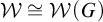 for the t.d.l.c. group G (and hence cannot be carried out for
$\alpha _{\mathcal {V}}$
for the t.d.l.c. group G (and hence cannot be carried out for
$\alpha _{\mathcal {V}}$
 ).
).
Claim 10.3.
$\alpha _{\mathcal {W}}$
 is a meet groupoid isomorphism.
It suffices to show that
$\alpha _{\mathcal {W}} = \widetilde \Phi $
 . To see this, let
$A_U\in \mathcal {W}$
. To see this, let
$A_U\in \mathcal {W}$
 . For the inclusion
$\widetilde \Phi (A) \subseteq \alpha _{\mathcal {W}}(A)$
. For the inclusion
$\widetilde \Phi (A) \subseteq \alpha _{\mathcal {W}}(A)$
 , if
$g \in A$
, if
$g \in A$
 then clearly
$ \Phi (g)(U)=gU = A$
then clearly
$ \Phi (g)(U)=gU = A$
 , so
$\Phi (g) \in \alpha _{\mathcal {W}}(A)$
, so
$\Phi (g) \in \alpha _{\mathcal {W}}(A)$
 . For the converse inclusion, suppose
$p_0(U)= A$
. For the converse inclusion, suppose
$p_0(U)= A$
 for
$p\in \widetilde G$
for
$p\in \widetilde G$
 , and let
$g = \Phi ^{-1}(p) $
, and let
$g = \Phi ^{-1}(p) $
 . Then
$g\in A$
. Then
$g\in A$
 because
$\Phi (g)(U)= p_0(U)= A$
because
$\Phi (g)(U)= p_0(U)= A$
 . This verifies the claim.
Let
$\Gamma \colon \widetilde {\mathcal {W}} \to \widetilde {\mathcal {V}}$
 be the “double dual” of the isomorphism
$\beta \colon \mathcal {W} \to \mathcal {V}$
be the “double dual” of the isomorphism
$\beta \colon \mathcal {W} \to \mathcal {V}$
 ; that is,
$\Gamma (A) = \{ \widetilde \beta (p) \colon \, p \in A\}$
; that is,
$\Gamma (A) = \{ \widetilde \beta (p) \colon \, p \in A\}$
 , where
$\widetilde \beta $
, where
$\widetilde \beta $
 is the dual of
$\beta $
is the dual of
$\beta $
 defined as in Equation (4) with
$\beta $
defined as in Equation (4) with
$\beta $
 in place of
$\theta $
in place of
$\theta $
 . Note that
$\Gamma $
. Note that
$\Gamma $
 is an isomorphism of meet groupoids.
Claim 10.4. The diagram
 commutes.
Hence
$\alpha _{\mathcal {V}}$
 is an isomorphism of meet groupoids.
To see this, if
$A_U \in \mathcal {W}$
 , then

where
$p^\beta :=\beta \circ f \circ \beta ^{-1} \oplus \beta \circ f^{-1} \circ \beta ^{-1}$
 , for
$p= f \oplus f^{-1}$
, for
$p= f \oplus f^{-1}$
 , similar to Equation (4).
Since G is autostable by hypothesis, and
$\Phi \colon G \to \widetilde G$
 is bicomputable,
$\widetilde G$
is bicomputable,
$\widetilde G$
 is autostable. Since
$\beta $
is autostable. Since
$\beta $
 is an isomorphism, we have
$\widetilde G \cong \widetilde H$
is an isomorphism, we have
$\widetilde G \cong \widetilde H$
 . Hence there is a bicomputable isomorphism
$ \widetilde G \to \widetilde H$
. Hence there is a bicomputable isomorphism
$ \widetilde G \to \widetilde H$
 . Inspecting the construction in the proof of the implication “
$\Leftarrow $
. Inspecting the construction in the proof of the implication “
$\Leftarrow $
 ” of Theorem 5.1 shows that there is a computable isomorphism
$\widetilde {\mathcal {W}} \to \widetilde {\mathcal {V}}$
” of Theorem 5.1 shows that there is a computable isomorphism
$\widetilde {\mathcal {W}} \to \widetilde {\mathcal {V}}$
 . So there is a computable isomorphism
$ {\mathcal {W}} \to {\mathcal {V}}$
. So there is a computable isomorphism
$ {\mathcal {W}} \to {\mathcal {V}}$
 , as required.
Remark 10.5 (Computable duality between t.d.l.c. groups and meet groupoids).
The post [Reference Nies38, Section 4] axiomatizes the class
$\mathbf M$
 of countable meet groupoids
$\mathcal {W}$
of countable meet groupoids
$\mathcal {W}$
 that are isomorphic to
$\mathcal {W}(G)$
that are isomorphic to
$\mathcal {W}(G)$
 for some t.d.l.c. group G. Note that Definition 5.2 of
$\mathcal {G}_{\text {comp}}( \mathcal {W})$
for some t.d.l.c. group G. Note that Definition 5.2 of
$\mathcal {G}_{\text {comp}}( \mathcal {W})$
 makes sense for any meet groupoid
$\mathcal {W}$
makes sense for any meet groupoid
$\mathcal {W}$
 with domain
${\mathbb {N}}$
with domain
${\mathbb {N}}$
 . Besides some basic algebraic axioms on meet groupoids (such as saying that different left cosets of the same subgroup are disjoint), one needs an axiom ensuring local compactness of
$\mathcal {G}_{\text {comp}}( \mathcal {W})$
. Besides some basic algebraic axioms on meet groupoids (such as saying that different left cosets of the same subgroup are disjoint), one needs an axiom ensuring local compactness of
$\mathcal {G}_{\text {comp}}( \mathcal {W})$
 : there is a subgroup K such that each subgroup
$U \subseteq K$
: there is a subgroup K such that each subgroup
$U \subseteq K$
 has only finitely many left cosets contained in K. Furthermore, one needs to say that the map
$\alpha _{\mathcal {W}} \colon \mathcal {W} \to \widetilde {\mathcal {W}}$
has only finitely many left cosets contained in K. Furthermore, one needs to say that the map
$\alpha _{\mathcal {W}} \colon \mathcal {W} \to \widetilde {\mathcal {W}}$
 in Claim 10.3 is onto. In general, this could fail: consider the meet groupoid obtained from a computable copy of
$\mathcal {W}({\mathbb {Z}}_p)$
in Claim 10.3 is onto. In general, this could fail: consider the meet groupoid obtained from a computable copy of
$\mathcal {W}({\mathbb {Z}}_p)$
 by deleting all cosets of subgroup of the form
$p^{2i+1} {\mathbb {Z}}_p$
by deleting all cosets of subgroup of the form
$p^{2i+1} {\mathbb {Z}}_p$
 : its double dual
$\mathcal {W}$
: its double dual
$\mathcal {W}$
 is isomorphic to
$\mathcal {W}({\mathbb {Z}}_p)$
is isomorphic to
$\mathcal {W}({\mathbb {Z}}_p)$
 . The required “completeness axiom” avoiding this situation, called CLC in [Reference Nies38, Section 4], states that if
$N \in \mathcal {W}$
. The required “completeness axiom” avoiding this situation, called CLC in [Reference Nies38, Section 4], states that if
$N \in \mathcal {W}$
 is normal (i.e., each left coset of N is also a right coset), and
$\mathcal {S} \subseteq L(N)$
is normal (i.e., each left coset of N is also a right coset), and
$\mathcal {S} \subseteq L(N)$
 is finite and closed under inverse and product, then there is a subgroup
$V \in \mathcal {W}$
is finite and closed under inverse and product, then there is a subgroup
$V \in \mathcal {W}$
 such that
$C \subseteq V \leftrightarrow C \in \mathcal {S}$
such that
$C \subseteq V \leftrightarrow C \in \mathcal {S}$
 . (These axioms are sufficiently simple to imply that
$\mathbf M$
. (These axioms are sufficiently simple to imply that
$\mathbf M$
 is an arithmetical class.) Using the methods to prove Criterion 10.2 one can proceed to showing that the operators
$\mathcal {W}_{\text {comp}}$
is an arithmetical class.) Using the methods to prove Criterion 10.2 one can proceed to showing that the operators
$\mathcal {W}_{\text {comp}}$
 and
$\mathcal {G}_{\text {comp}}$
and
$\mathcal {G}_{\text {comp}}$
 , restricted to the Haar computable meet groupoids in
$\mathbf M$
, restricted to the Haar computable meet groupoids in
$\mathbf M$
 , are inverses of each other. That is, composing one with the other leads to a computable copy of the original structure that is computably isomorphic to it.
Theorem 10.6. The computably t.d.l.c. groups
${\mathbb {Q}}_p$
 and
${\mathbb {Z}} \ltimes {\mathbb {Q}}_p$
and
${\mathbb {Z}} \ltimes {\mathbb {Q}}_p$
 are autostable.
Proof. In Proposition 4.9 we obtained a Haar computable copy
$\mathcal {W}$
 of the meet groupoid
$\mathcal {W}({\mathbb {Q}}_p)$
of the meet groupoid
$\mathcal {W}({\mathbb {Q}}_p)$
 . Recall that the elements of
$\mathcal {W}$
. Recall that the elements of
$\mathcal {W}$
 are given as cosets
$D_{r,a}=\pi _r^{-1}(a)$
are given as cosets
$D_{r,a}=\pi _r^{-1}(a)$
 where
$r\in {\mathbb {Z}}$
where
$r\in {\mathbb {Z}}$
 ,
$\pi _r \colon {\mathbb {Z}}_p \to C_{p^\infty }$
,
$\pi _r \colon {\mathbb {Z}}_p \to C_{p^\infty }$
 is the canonical projection with kernel
$U_r =p^{r} {\mathbb {Z}}_p$
is the canonical projection with kernel
$U_r =p^{r} {\mathbb {Z}}_p$
 , and
$a \in C_{p^\infty }$
, and
$a \in C_{p^\infty }$
 .
.
By the criterion above, it suffices to show that any Haar computable copy
$\widetilde {\mathcal {W}}$
 of
$\mathcal {W}({\mathbb {Q}}_p)$
of
$\mathcal {W}({\mathbb {Q}}_p)$
 is computably isomorphic to
$\mathcal {W}$
is computably isomorphic to
$\mathcal {W}$
 . By hypothesis on
$\widetilde {\mathcal {W}}$
. By hypothesis on
$\widetilde {\mathcal {W}}$
 there is an isomorphism
$\Gamma \colon \mathcal {W} \to \widetilde {\mathcal {W}}$
there is an isomorphism
$\Gamma \colon \mathcal {W} \to \widetilde {\mathcal {W}}$
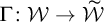 . Let
$\widetilde U_r = \Gamma (U_r)$
. Let
$\widetilde U_r = \Gamma (U_r)$
 for
$r\in {\mathbb {Z}}$
for
$r\in {\mathbb {Z}}$
 . We will construct a computable isomorphism
$\Delta \colon \mathcal {W} \to \widetilde {\mathcal {W}}$
. We will construct a computable isomorphism
$\Delta \colon \mathcal {W} \to \widetilde {\mathcal {W}}$
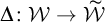 which agrees with
$\Gamma $
which agrees with
$\Gamma $
 on the set
$\{U_r\colon \, r\in {\mathbb {Z}}\}$
on the set
$\{U_r\colon \, r\in {\mathbb {Z}}\}$
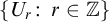 . First we show that from r one can compute the subgroup
$\widetilde U_r \in \widetilde {\mathcal {W}}$
. First we show that from r one can compute the subgroup
$\widetilde U_r \in \widetilde {\mathcal {W}}$
 .
.
-
(a) If $\widetilde U_r$
has been determined,
$r\ge 0$
, compute
$\widetilde U_{r+1}$
by searching for the unique subgroup in
$\widetilde {\mathcal {W}}$
that has index p in
$\widetilde U_r$
. -
(b) If $\widetilde U_r$
has been determined,
$r\le 0$
, compute
$\widetilde U_{r-1}$
by searching for the unique subgroup in
$\widetilde {\mathcal {W}}$
such that
$\widetilde U_r$
has index p in it.


The shift homeomorphism
$S\colon {\mathbb {Q}}_p \to {\mathbb {Q}}_p$
 is defined by
$S(x)= p x$
is defined by
$S(x)= p x$
 . Note that
$B \to S(B)$
. Note that
$B \to S(B)$
 is an automorphism of the meet groupoid
$\mathcal {W}$
is an automorphism of the meet groupoid
$\mathcal {W}$
 . Using the notation of Proposition 4.9 (recalled above), for each
$\alpha \in {\mathbb {Q}}_p, r \in {\mathbb {Z}}$
. Using the notation of Proposition 4.9 (recalled above), for each
$\alpha \in {\mathbb {Q}}_p, r \in {\mathbb {Z}}$
 , one has
$\pi _{r+1}(S(\alpha ))=\pi _r(\alpha )$
, one has
$\pi _{r+1}(S(\alpha ))=\pi _r(\alpha )$
 , and hence for each
$a \in C_{p^\infty }$
, and hence for each
$a \in C_{p^\infty }$
 ,
,

We show that S is definable within
$\mathcal {W}$
 by an existential formula using subgroups
$U_r$
by an existential formula using subgroups
$U_r$
 as parameters. Recall that given a meet groupoid
$\mathcal {W}$
as parameters. Recall that given a meet groupoid
$\mathcal {W}$
 , by
$L(U)$
, by
$L(U)$
 we denote the set of left cosets of a subgroup U. For
$D \in L(U_r)$
we denote the set of left cosets of a subgroup U. For
$D \in L(U_r)$
 we write
$D^k$
we write
$D^k$
 for
$D \cdot \dots \cdot D$
for
$D \cdot \dots \cdot D$
 (with k factors), noting that this is defined, and in
$L(U_r)$
(with k factors), noting that this is defined, and in
$L(U_r)$
 .
.
Claim 10.7. Let
$B \in L(U_r)$
 and
$ C\in L(U_{r+1})$
and
$ C\in L(U_{r+1})$
 . Then

“
$\Leftarrow $
 ”: If
$x \in C$
”: If
$x \in C$
 then
$x = py$
then
$x = py$
 for some
$y \in B$
for some
$y \in B$
 , so
$x \in S(B)$
, so
$x \in S(B)$
 . So
$C \subseteq S(B)$
. So
$C \subseteq S(B)$
 and hence
$C= S(B)$
and hence
$C= S(B)$
 given that
$S(B)\in L(U_{r+1})$
given that
$S(B)\in L(U_{r+1})$
 .
.
“
$\Rightarrow $
 ”: Let
$x\in C$
”: Let
$x\in C$
 , so
$x = S(y)$
, so
$x = S(y)$
 for some
$y \in B$
for some
$y \in B$
 . Let
$y \in D$
. Let
$y \in D$
 where
$D \in L(U_{r+1})$
where
$D \in L(U_{r+1})$
 . Then
$D\subseteq B$
. Then
$D\subseteq B$
 . Since
$D^p \cap C \neq \emptyset $
. Since
$D^p \cap C \neq \emptyset $
 , these two (left) cosets of
$U_{r+1}$
, these two (left) cosets of
$U_{r+1}$
 coincide. This shows the claim.
We use this to show that the function
$\widetilde S=\Gamma \circ S \circ \Gamma ^{-1} $
 defined on
$\widetilde {\mathcal {W}}$
defined on
$\widetilde {\mathcal {W}}$
 is computable. Since
$\Gamma ( U_r)= \widetilde U_r$
is computable. Since
$\Gamma ( U_r)= \widetilde U_r$
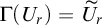 , (
$r \in {\mathbb {Z}}$
, (
$r \in {\mathbb {Z}}$
 ),
$\widetilde S $
),
$\widetilde S $
 satisfies the claim when replacing the
$U_r$
satisfies the claim when replacing the
$U_r$
 by the
$\widetilde U_r$
by the
$\widetilde U_r$
 . Since the meet groupoid
$\widetilde {\mathcal {W}}$
. Since the meet groupoid
$\widetilde {\mathcal {W}}$
 is computable, given
$B \in \widetilde {\mathcal {W}}$
is computable, given
$B \in \widetilde {\mathcal {W}}$
 , one can search
$\widetilde {\mathcal {W}}$
, one can search
$\widetilde {\mathcal {W}}$
 for a witness
$D\in L(\widetilde U_{r+1})$
for a witness
$D\in L(\widetilde U_{r+1})$
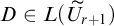 as on the right hand side, and then output
$C= \widetilde S(B)$
as on the right hand side, and then output
$C= \widetilde S(B)$
 . So the function
$\widetilde S$
. So the function
$\widetilde S$
 is computable.
We build the computable isomorphism
$\Delta \colon \mathcal {W} \to \widetilde {\mathcal {W}}$
 in four phases. The first three phases build a computable isomorphism
$L( U_0) \to L(\widetilde U_0)$
in four phases. The first three phases build a computable isomorphism
$L( U_0) \to L(\widetilde U_0)$
 , where
$L(\widetilde U_0) \subseteq \widetilde {\mathcal {W}}$
, where
$L(\widetilde U_0) \subseteq \widetilde {\mathcal {W}}$
 denotes the group of left cosets of
$\widetilde U_0$
denotes the group of left cosets of
$\widetilde U_0$
 . (This group is isomorphic to
$C_{p^\infty }$
. (This group is isomorphic to
$C_{p^\infty }$
 , so this amounts to defining a computable isomorphism between two computable copies of
$C_{p^\infty }$
, so this amounts to defining a computable isomorphism between two computable copies of
$C_{p^\infty }$
 .) The last phase extends this isomorphism to all of
$ \mathcal {W}$
.) The last phase extends this isomorphism to all of
$ \mathcal {W}$
 , using that
$\widetilde S$
, using that
$\widetilde S$
 is an automorphism of
$\widetilde {\mathcal {W}}$
is an automorphism of
$\widetilde {\mathcal {W}}$
 .
.
For
$q \in {\mathbb {Z}}[1/p] $
 we write
$[q]= {\mathbb {Z}} + q \in C_{p^\infty }$
we write
$[q]= {\mathbb {Z}} + q \in C_{p^\infty }$
 . We define
$\widetilde D_{r,[q]}= \Delta (D_{r,a})$
. We define
$\widetilde D_{r,[q]}= \Delta (D_{r,a})$
 for
$r \in {\mathbb {Z}}, q \in {\mathbb {Z}}[1/p] $
for
$r \in {\mathbb {Z}}, q \in {\mathbb {Z}}[1/p] $

-
(a) Let $\widetilde D_{0, [p^{-1}]}$
be an element of order p in
$L(\widetilde U_0) $
. -
(b) Recursively, for $m>0$
let
$\widetilde D_{0, [p^{-m}]}$
be an element of order
$p^m$
in
$L(\widetilde U_0) $
such that
$(\widetilde D_{0, [p^{-m}]})^p = \widetilde D_{0, [p^{-m+1}]}$
. -
(c) For $a = [kp^{-m}]$
where
$0 \le k <p^m$
and
$p $
does not divide k, let
$\widetilde D_{0, a} = (\widetilde D_{0, [p^{-m}]})^k$
. -
(d) For $r \in {\mathbb {Z}} -\{0\}$
let
$\widetilde D_{r,a} =\widetilde S^r (\widetilde D_{0,a})$
.





One can easily verify that
$\Delta \colon \mathcal {W} \to \widetilde {\mathcal {W}}$
 is computable and preserves the meet groupoid operations. To verify that
$\Delta $
is computable and preserves the meet groupoid operations. To verify that
$\Delta $
 is onto, let
$B \in \widetilde {\mathcal {W}}$
is onto, let
$B \in \widetilde {\mathcal {W}}$
 . We have
$B \in L(\widetilde U_r)$
. We have
$B \in L(\widetilde U_r)$
 for some r. There is a least m such that
$B= (\widetilde D_{r, [p^{-m}]})^k$
for some r. There is a least m such that
$B= (\widetilde D_{r, [p^{-m}]})^k$
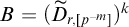 for some
$k< p^m$
for some
$k< p^m$
 . Then p does not divide k, so
$B= \widetilde D_{r, [kp^{-m}]}$
. Then p does not divide k, so
$B= \widetilde D_{r, [kp^{-m}]}$
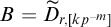 .
.
We next treat the case of
$G={\mathbb {Z}} \ltimes {\mathbb {Q}}_p$
 . Let
$\mathcal {V}$
. Let
$\mathcal {V}$
 be the Haar computable copy of
$\mathcal {W}(G)$
be the Haar computable copy of
$\mathcal {W}(G)$
 obtained in Proposition 4.9, and let
$\widetilde {\mathcal {V}}$
obtained in Proposition 4.9, and let
$\widetilde {\mathcal {V}}$
 be a further Haar computable copy of
$\mathcal {W}(G)$
be a further Haar computable copy of
$\mathcal {W}(G)$
 . Using the notation of Proposition 4.9, let

We list some properties of these elements of
$\mathcal {V}$
 that will be needed shortly. Note that we can view
$\mathcal {W}$
that will be needed shortly. Note that we can view
$\mathcal {W}$
 as embedded into
$\mathcal {V}$
as embedded into
$\mathcal {V}$
 by identifying
$\langle r,a\rangle $
by identifying
$\langle r,a\rangle $
 with
$\langle 0,r,a\rangle $
with
$\langle 0,r,a\rangle $
 . Also note that
$E_{z,r,a} \colon U_{r-z} \to U_r$
. Also note that
$E_{z,r,a} \colon U_{r-z} \to U_r$
 (using the category notation of Remark 4.4). Since
$D_{r+1, a} \subseteq D_{r,pa}$
(using the category notation of Remark 4.4). Since
$D_{r+1, a} \subseteq D_{r,pa}$
 , we have

Furthermore,

By hypothesis on
$\widetilde {\mathcal {V}}$
 , there is a meet groupoid isomorphism
$\overline \Gamma \colon \mathcal {V} \to \widetilde {\mathcal {V}}$
, there is a meet groupoid isomorphism
$\overline \Gamma \colon \mathcal {V} \to \widetilde {\mathcal {V}}$
 . Since G has no compact open subgroups besides the ones present in
$\mathcal {W}({\mathbb {Q}}_p)$
. Since G has no compact open subgroups besides the ones present in
$\mathcal {W}({\mathbb {Q}}_p)$
 , the family
$(\widetilde U_r)_{r \in {\mathbb {Z}}}$
, the family
$(\widetilde U_r)_{r \in {\mathbb {Z}}}$
 , where
$\widetilde U_r = \overline \Gamma (U_r)$
, where
$\widetilde U_r = \overline \Gamma (U_r)$
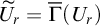 , is computable in
$\widetilde {\mathcal {V}}$
, is computable in
$\widetilde {\mathcal {V}}$
 by the same argument as before. The set of elements A of
$\widetilde {\mathcal {V}}$
by the same argument as before. The set of elements A of
$\widetilde {\mathcal {V}}$
 that are a left and a right coset of the same subgroup is computable by checking whether
$A^{-1} \cdot A= A \cdot A^{-1}$
that are a left and a right coset of the same subgroup is computable by checking whether
$A^{-1} \cdot A= A \cdot A^{-1}$
 . The operations of
$\widetilde {\mathcal {V}}$
. The operations of
$\widetilde {\mathcal {V}}$
 induce a Haar computable meet groupoid
$\widetilde {\mathcal {W}}$
induce a Haar computable meet groupoid
$\widetilde {\mathcal {W}}$
 on this set. Clearly the restricted map
$\Gamma =\overline \Gamma \mid \mathcal {W}$
on this set. Clearly the restricted map
$\Gamma =\overline \Gamma \mid \mathcal {W}$
 is an isomorphism
$\mathcal {W} \to \widetilde {\mathcal {W}}$
is an isomorphism
$\mathcal {W} \to \widetilde {\mathcal {W}}$
 . So by the case of
${\mathbb {Q}}_p$
. So by the case of
${\mathbb {Q}}_p$
 , there is a computable isomorphism
$\Delta \colon \mathcal {W} \to \widetilde {\mathcal {W}}$
, there is a computable isomorphism
$\Delta \colon \mathcal {W} \to \widetilde {\mathcal {W}}$
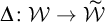 .
.
We will extend
$\Delta $
 to a computable isomorphism
$\overline \Delta \colon \mathcal {V} \to \widetilde {\mathcal {V}}$
to a computable isomorphism
$\overline \Delta \colon \mathcal {V} \to \widetilde {\mathcal {V}}$
 . The following summarizes the setting:

In five phases we define a computable family
$\widetilde E_{z,r,a}$
 (
$z, r \in {\mathbb {Z}}, a \in C_{p^\infty }$
(
$z, r \in {\mathbb {Z}}, a \in C_{p^\infty }$
 ), and then let
$\overline \Delta (E_{z,r,a})= \widetilde E_{z,r,a}$
), and then let
$\overline \Delta (E_{z,r,a})= \widetilde E_{z,r,a}$
 . As before write
$\widetilde D_{r,a} = \Delta ( D_{r,a})$
. As before write
$\widetilde D_{r,a} = \Delta ( D_{r,a})$
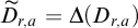 .
.
-
(a) Let $\widetilde E_{0,r,a} = \widetilde D_{r,a}$
. Choose
$F_0:= \widetilde E_{-1,0,0} \colon \widetilde U_1 \to \widetilde U_0$
. -
(b) Compute $F_r:=\widetilde E_{-1,r,0}\colon U_{r+1} \to U_r$
by recursion on
$|r|$
, where
$r \in {\mathbb {Z}}$
, in such a way that
$\widetilde F_{r+1} \subseteq \widetilde F_r$
for each
$r \in {\mathbb {Z}}$
; this is possible by (6) and since
$\mathcal {V} \cong \widetilde {\mathcal {V}}$
via
$\overline \Gamma $
. -
(c) For $z < -1$
, compute
$ \widetilde E_{z,r,0}\colon U_{r-z} \to U_r$
as follows: $$ \begin{align*} \widetilde E_{z,r,0}= F_{r-z-1} \cdot F_{r-z-2} \cdot \dots \cdot F_r. \end{align*} $$
-
(d) For $z>0$
let
$\widetilde E_{z,r,0}= (\widetilde E_{-z, r-z, 0 })^{-1}$
; this is enforced by (7). -
(e) Let $\widetilde E_{z,r,a}= \widetilde E_{z,r,0} \cdot \widetilde D_{r,a}$
.
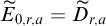






One verifies that
$\overline \Delta $
 preserves the meet groupoid operations (we omit the formal detail). To show that
$\overline \Delta $
preserves the meet groupoid operations (we omit the formal detail). To show that
$\overline \Delta $
 is onto, suppose that
$\widetilde E \in \mathcal {V}$
is onto, suppose that
$\widetilde E \in \mathcal {V}$
 is given. Then
$\widetilde E = \Gamma (E_{z,r,a})$
is given. Then
$\widetilde E = \Gamma (E_{z,r,a})$
 for some
$z,r,a$
for some
$z,r,a$
 . By (6) we may assume that
$z<0$
. By (6) we may assume that
$z<0$
 . Then
$ E_{z,r,0}= \prod _{i=1}^{-z}E_{-1,r-z-i,0} $
. Then
$ E_{z,r,0}= \prod _{i=1}^{-z}E_{-1,r-z-i,0} $
 as above. So, writing
$F_s$
as above. So, writing
$F_s$
 for
$\widetilde E_{-1,s,0}$
for
$\widetilde E_{-1,s,0}$
 , we have
$\Gamma (E_{z,r,0})= \prod _{i=1}^{-z}F_{r-z-i} \widetilde D_{r-z-i, a_i}$
, we have
$\Gamma (E_{z,r,0})= \prod _{i=1}^{-z}F_{r-z-i} \widetilde D_{r-z-i, a_i}$
 for some
$a_i \in C_{p^\infty }$
for some
$a_i \in C_{p^\infty }$
 .
.
Note that
$\widetilde S(D)= F \cdot D \cdot F^{-1}$
 for each
$D \in L(\widetilde U_r) \cap \widetilde {\mathcal {W}}$
for each
$D \in L(\widetilde U_r) \cap \widetilde {\mathcal {W}}$
 and
$F \colon \widetilde U_{r+1} \to \widetilde U_r$
and
$F \colon \widetilde U_{r+1} \to \widetilde U_r$
 . For, the analogous statement clearly holds in
$\mathcal {V}$
. For, the analogous statement clearly holds in
$\mathcal {V}$
 ; then one uses that
$\widetilde S=\Gamma \circ S \circ \Gamma ^{-1} $
; then one uses that
$\widetilde S=\Gamma \circ S \circ \Gamma ^{-1} $
 , and that
$\overline \Gamma \colon \mathcal {V} \to \widetilde {\mathcal {V}}$
, and that
$\overline \Gamma \colon \mathcal {V} \to \widetilde {\mathcal {V}}$
 is an isomorphism. Since
$\widetilde D_{r+1,a}= \widetilde S(\widetilde D_{r,a})$
is an isomorphism. Since
$\widetilde D_{r+1,a}= \widetilde S(\widetilde D_{r,a})$
 , we may conclude that
$\widetilde D_{r+1, a}\cdot F = F \cdot D_{r,a}$
, we may conclude that
$\widetilde D_{r+1, a}\cdot F = F \cdot D_{r,a}$
 for each such F. We can use these “quasi-commutation relations” to simplify the expression
$\prod _{i=1}^{-z}F_{r-z-i} \widetilde D_{r-z-i, a_i}$
for each such F. We can use these “quasi-commutation relations” to simplify the expression
$\prod _{i=1}^{-z}F_{r-z-i} \widetilde D_{r-z-i, a_i}$
 to
$\widetilde E_{z,r,0} \widetilde D_{r,b}$
to
$\widetilde E_{z,r,0} \widetilde D_{r,b}$
 for some
$b \in C_{p^\infty }$
for some
$b \in C_{p^\infty }$
 . Hence
$\widetilde E = \widetilde E_{z,r,0} \widetilde D_{r,b} \widetilde D_{r,a}$
. Hence
$\widetilde E = \widetilde E_{z,r,0} \widetilde D_{r,b} \widetilde D_{r,a}$
 . This shows that
$\widetilde E$
. This shows that
$\widetilde E$
 is in the range of
$\overline \Delta $
is in the range of
$\overline \Delta $
 , as required.
Appendix A (with George Willis): A non-computable scale function.
Let
$\mathbb F$
 be some finite field; for notational simplicity we will assume that
$|\mathbb F|=2$
be some finite field; for notational simplicity we will assume that
$|\mathbb F|=2$
 . We write H for the additive group of
${\mathbb {F}}((t))$
. We write H for the additive group of
${\mathbb {F}}((t))$
 . The group
${Aut}(H)$
. The group
${Aut}(H)$
 is equipped with the usual Braconnier topology recalled before Proposition 5.7. For
$\pi \in {Aut}(H)$
is equipped with the usual Braconnier topology recalled before Proposition 5.7. For
$\pi \in {Aut}(H)$
 let
$s(\pi ) = \min _V \{|\pi (V) \colon V \cap \pi (V)| $
let
$s(\pi ) = \min _V \{|\pi (V) \colon V \cap \pi (V)| $
 where as usual V ranges over compact open subgroups. Willis [Reference Willis60, Example 1] showed that
$s \colon {Aut}(H) \to {\mathbb {N}}^+$
where as usual V ranges over compact open subgroups. Willis [Reference Willis60, Example 1] showed that
$s \colon {Aut}(H) \to {\mathbb {N}}^+$
 is not continuous. He defined automorphisms
$\pi _t (t \in {\mathbb {N}})$
is not continuous. He defined automorphisms
$\pi _t (t \in {\mathbb {N}})$
 and
$\pi $
and
$\pi $
 of
$H $
of
$H $
 such that
$\lim _t \pi _t = \pi $
such that
$\lim _t \pi _t = \pi $
 ,
$s(\pi _t)= 1$
,
$s(\pi _t)= 1$
 and
$s(\pi )=2$
and
$s(\pi )=2$
 . Starting from his example we show the following.
Theorem A.1 (with George Willis).
There is a computable Baire presentation
$(T, {Mult}, {Inv})$
 of a t.d.l.c. group G and a computable sequence of paths
$(\overline g_i)_{i \in {\mathbb {N}}^+}$
of a t.d.l.c. group G and a computable sequence of paths
$(\overline g_i)_{i \in {\mathbb {N}}^+}$
 on T such that the function
$i \mapsto s(\overline g_i)$
on T such that the function
$i \mapsto s(\overline g_i)$
 is non-computable. Moreover, G is elementary in the sense of [Reference Wesolek56].
Proof. We begin with a brief outline. Let
$\mathcal {K}\subseteq {\mathbb {N}} $
 denote the usual halting problem, a standard recursively enumerable, undecidable set in computability theory. Uniformly in
$i\in {\mathbb {N}}^+$
denote the usual halting problem, a standard recursively enumerable, undecidable set in computability theory. Uniformly in
$i\in {\mathbb {N}}^+$
 we will build a computably t.d.l.c. group
$G_i$
we will build a computably t.d.l.c. group
$G_i$
 with a computable element
$g_i$
with a computable element
$g_i$
 so that
$s(g_i)= 2$
so that
$s(g_i)= 2$
 if
$i \not \in \mathcal {K}$
if
$i \not \in \mathcal {K}$
 , and
$s(g_i)=1$
, and
$s(g_i)=1$
 else. Along with
$G_i$
else. Along with
$G_i$
 , uniformly in i we determine a compact open subgroup
$U_i$
, uniformly in i we determine a compact open subgroup
$U_i$
 . Then the statement of the theorem holds for the t.d.l.c. group
$G=\bigoplus _{i\in {\mathbb {N}}^+} (G_i, U_i) $
. Then the statement of the theorem holds for the t.d.l.c. group
$G=\bigoplus _{i\in {\mathbb {N}}^+} (G_i, U_i) $
 , with the computable presentation according to the proof of Proposition 9.5, where
$\overline g_i$
, with the computable presentation according to the proof of Proposition 9.5, where
$\overline g_i$
 is the image of
$g_i$
is the image of
$g_i$
 under the canonical embedding
$G_i \to G$
under the canonical embedding
$G_i \to G$
 .
.
We let
$G_i $
 be the split extension
${\mathbb {Z}} \ltimes H$
be the split extension
${\mathbb {Z}} \ltimes H$
 for the action of
${\mathbb {Z}}$
for the action of
${\mathbb {Z}}$
 corresponding to an automorphism
$\widehat \beta _i$
corresponding to an automorphism
$\widehat \beta _i$
 of H. To define
$\widehat \beta _i$
of H. To define
$\widehat \beta _i$
 we combine the technique of Willis with an argument from computability theory. Informally speaking, if a number i enters
$\mathcal {K}$
we combine the technique of Willis with an argument from computability theory. Informally speaking, if a number i enters
$\mathcal {K}$
 at a stage t, the approximation of
$\widehat \beta _i$
at a stage t, the approximation of
$\widehat \beta _i$
 changes from “following”
$\pi $
changes from “following”
$\pi $
 to “following”
$\pi _t$
to “following”
$\pi _t$
 . We have
$s_G(\overline g_i)= s_H(\widehat \beta _i)$
. We have
$s_G(\overline g_i)= s_H(\widehat \beta _i)$
 where
$g_i \in G_i$
where
$g_i \in G_i$
 is the element such that conjugation by
$g_i $
is the element such that conjugation by
$g_i $
 induces the automorphism
$\overline \beta _i$
induces the automorphism
$\overline \beta _i$
 on H.
on H.
We proceed to the details. We use the computable Baire presentation
$(Q, {Mult}, {Inv})$
 of H given by the proof of Proposition 7.8. Recall that strings on Q other than the root are of the form
$r\sigma $
of H given by the proof of Proposition 7.8. Recall that strings on Q other than the root are of the form
$r\sigma $
 where
$r\in {\mathbb {N}}$
where
$r\in {\mathbb {N}}$
 ,
$\sigma \in \{0,1\}^*$
,
$\sigma \in \{0,1\}^*$
 is a binary string, and if
$r>0$
is a binary string, and if
$r>0$
 then
$\sigma $
then
$\sigma $
 does not start with
$0$
does not start with
$0$
 . We think of
$r\sigma $
. We think of
$r\sigma $
 as denoting the formal Laurent polynomial
$x^{-r} \sum _{0 \le k< |\sigma |} \sigma (k) x^k$
as denoting the formal Laurent polynomial
$x^{-r} \sum _{0 \le k< |\sigma |} \sigma (k) x^k$
 ; note that
$\sigma $
; note that
$\sigma $
 is allowed to end in
$0$
is allowed to end in
$0$
 .
.
For
$c\in {\mathbb {N}}$
 , we say that a permutation
$\alpha $
, we say that a permutation
$\alpha $
 of
${\mathbb {Z}}$
of
${\mathbb {Z}}$
 is c-bounded if
$|\alpha (z)-z| \le c$
is c-bounded if
$|\alpha (z)-z| \le c$
 for each
$z \in {\mathbb {Z}}$
for each
$z \in {\mathbb {Z}}$
 . In this case the function
$\widehat \alpha $
. In this case the function
$\widehat \alpha $
 defined on H by

is a continuous automorphism of H.
Claim A.2. Let
$\alpha $
 be a computable c-bounded permutation of
${\mathbb {Z}}$
be a computable c-bounded permutation of
${\mathbb {Z}}$
 . Then
$\widehat \alpha \colon [Q] \to [Q]$
. Then
$\widehat \alpha \colon [Q] \to [Q]$
 is computable, uniformly in c and a Turing machine index for computing
$\alpha $
is computable, uniformly in c and a Turing machine index for computing
$\alpha $
 .
.
We verify this by defining a monotonic computable function L on the tree Q according to Remark 6.5. For
$r\in {\mathbb {N}}$
 and a binary string
$\sigma $
and a binary string
$\sigma $
 such that
$|\sigma | \ge 2c+1$
such that
$|\sigma | \ge 2c+1$
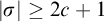 , we declare that
$L(r\sigma )= s\tau $
, we declare that
$L(r\sigma )= s\tau $
 where
where
-
(a) $-s$
is the minimum of
$0$
and the values
$\alpha (k-r)$
,
$k \le 2c+1$
such that
$\sigma (k) \neq 0$
; if there is no such value (and hence
$r=0$
) let
$s=0$
; -
(b) $\tau $
is obtained by searching for the maximal
$\ell = |\tau | $
such that for each
$k< \ell $
the value $$ \begin{align*} \tau(k)= \sigma(\alpha^{-1}(k-s)+r)\end{align*} $$is defined.


If
$s>0$
 then
$\tau (0)= \sigma (k)= 1$
then
$\tau (0)= \sigma (k)= 1$
 where
$k-r$
where
$k-r$
 is the position at which the minimal value is taken in (a), so indeed
$s\tau \in Q$
is the position at which the minimal value is taken in (a), so indeed
$s\tau \in Q$
 . Clearly L is monotonic. Since
$\alpha $
. Clearly L is monotonic. Since
$\alpha $
 is c-bounded, given
$r \in {\mathbb {N}}$
is c-bounded, given
$r \in {\mathbb {N}}$
 and
$\sigma $
and
$\sigma $
 with
$|\sigma | \ge 2c+1$
with
$|\sigma | \ge 2c+1$
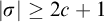 , we have
$L(r\sigma )= s\tau $
, we have
$L(r\sigma )= s\tau $
 for some
$s\in {\mathbb {N}}$
for some
$s\in {\mathbb {N}}$
 and
$\tau $
and
$\tau $
 such that
$|\tau | \ge |\sigma | -c$
such that
$|\tau | \ge |\sigma | -c$
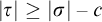 . Using this, one verifies that L is as required. This shows the claim.
Since
$\mathcal {K}$
 is r.e.,
$\mathcal {K} = \bigcup _t \mathcal {K}_t$
is r.e.,
$\mathcal {K} = \bigcup _t \mathcal {K}_t$
 for a computable sequence of strong indices for finite subsets of
${\mathbb {N}}$
for a computable sequence of strong indices for finite subsets of
${\mathbb {N}}$
 . For technical reasons we will assume that
$\mathcal {K}_t- \mathcal {K}_{t-1} \neq \emptyset $
. For technical reasons we will assume that
$\mathcal {K}_t- \mathcal {K}_{t-1} \neq \emptyset $
 implies that
$t $
implies that
$t $
 is even. We also let
$\mathcal {K}_t = \emptyset $
is even. We also let
$\mathcal {K}_t = \emptyset $
 for
$t<0$
for
$t<0$
 . The following defines a computable function
${\mathbb {N}}^+ \times {\mathbb {Z}} \to {\mathbb {Z}}$
. The following defines a computable function
${\mathbb {N}}^+ \times {\mathbb {Z}} \to {\mathbb {Z}}$
 via
$\langle i, t \rangle \mapsto \beta _i(t)$
via
$\langle i, t \rangle \mapsto \beta _i(t)$
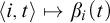 :
:

If
$i \not \in \mathcal {K}$
 then
$\beta _i$
then
$\beta _i$
 is the permutation of
${\mathbb {Z}}$
is the permutation of
${\mathbb {Z}}$
 that adds 2 to even numbers, and subtracts 2 from odd numbers. So
$s(\widehat \beta _i)=2$
that adds 2 to even numbers, and subtracts 2 from odd numbers. So
$s(\widehat \beta _i)=2$
 . If t is least such that
$i \in \mathcal {K}_t$
. If t is least such that
$i \in \mathcal {K}_t$
 then the nontrivial cycle of
$\beta _i$
then the nontrivial cycle of
$\beta _i$
 “turns around” at position t. Hence
$\widehat \beta _i$
“turns around” at position t. Hence
$\widehat \beta _i$
 leaves invariant the compact open subgroup consisting of the Laurent series that begin at position
$t+2$
leaves invariant the compact open subgroup consisting of the Laurent series that begin at position
$t+2$
 . So
$s(\widehat \beta _i)=1$
. So
$s(\widehat \beta _i)=1$
 .
.
Now let
$G_i = {\mathbb {Z}} \ltimes _{\gamma _i} H$
 , where
$\gamma _i$
, where
$\gamma _i$
 is the action
${\mathbb {Z}} \times H \to H$
is the action
${\mathbb {Z}} \times H \to H$
 given by
$\gamma _i(z,h) = \overline \beta _i^{z}(h)$
given by
$\gamma _i(z,h) = \overline \beta _i^{z}(h)$
 . Let
${\mathbb {Z}}$
. Let
${\mathbb {Z}}$
 have a computable Baire presentation according to Proposition 7.4. By Claim A.2,
$\gamma _i$
have a computable Baire presentation according to Proposition 7.4. By Claim A.2,
$\gamma _i$
 is computable. So the proof of Proposition 9.3 yields a computable Baire presentation of
$G_i$
is computable. So the proof of Proposition 9.3 yields a computable Baire presentation of
$G_i$
 . Note that
$U= \mathbb F[[t]]$
. Note that
$U= \mathbb F[[t]]$
 is a compact open subgroup of each
$G_i$
is a compact open subgroup of each
$G_i$
 . All the assertions in this paragraph hold uniformly in i.
Let
$g_i$
 be the generator of
${\mathbb {Z}}$
be the generator of
${\mathbb {Z}}$
 in
$G_i$
in
$G_i$
 whose conjugation action on H induces
$\beta _i$
whose conjugation action on H induces
$\beta _i$
 . Then
$s_{G_i}(g_i) = s_H(\widehat \beta _i)$
. Then
$s_{G_i}(g_i) = s_H(\widehat \beta _i)$
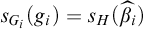 because
$G_i$
because
$G_i$
 and H have the same compact open subgroups.
Let
$G= (T, {Mult}, {Inv}) $
 be the computable Baire presentation of the local direct product
$G=\bigoplus _{i\in {\mathbb {N}}^+} (G_i, U) $
be the computable Baire presentation of the local direct product
$G=\bigoplus _{i\in {\mathbb {N}}^+} (G_i, U) $
 obtained in the proof of Proposition 9.5. It is clear that the sequence
$(\overline g_i)$
obtained in the proof of Proposition 9.5. It is clear that the sequence
$(\overline g_i)$
 of paths of T such that
$\overline g_i$
of paths of T such that
$\overline g_i$
 represents
$g_i$
represents
$g_i$
 viewed as an element of G is uniformly computable. It is easy to check that
$s_G(\overline g_i) = s_{G_i}(g_i)$
viewed as an element of G is uniformly computable. It is easy to check that
$s_G(\overline g_i) = s_{G_i}(g_i)$
 for each i. (The canonical projection
$G \to G_i$
for each i. (The canonical projection
$G \to G_i$
 is open, and to each compact open subgroup
$V_i$
is open, and to each compact open subgroup
$V_i$
 of
$G_i$
of
$G_i$
 corresponds a compact open subgroup W of G where
$W = \prod _{k \in {\mathbb {N}}^+} V_k$
corresponds a compact open subgroup W of G where
$W = \prod _{k \in {\mathbb {N}}^+} V_k$
 with
$V_k= U$
with
$V_k= U$
 for
$k \neq i$
for
$k \neq i$
 .) Thus
$s_G(\overline g_i ) = 1 $
.) Thus
$s_G(\overline g_i ) = 1 $
 iff
$i \in \mathcal {K}$
iff
$i \in \mathcal {K}$
 , as required.
Appendix B: Abelian t.d.l.c. groups.
Our work [Reference Lupini, Melnikov and Nies26], joint with Lupini, studies locally compact abelian groups with computable presentations. In particular, we investigate the algorithmic content of Pontryagin–van Kampen duality for such groups. Each abelian t.d.l.c. group is procountable, i.e., an inverse limit of countable groups. This enables us in [Reference Lupini, Melnikov and Nies26] to use a notion of computable presentation for t.d.l.c. abelian groups convenient for the given context. This notion, which in the present article we will call a computably procountable presentation with effectively finite kernels, is reviewed in Definition B.3 below. The main purpose of this short section is to show that the definition of computably t.d.l.c. abelian groups in [Reference Lupini, Melnikov and Nies26] is equivalent to the one given here.
B.1 Procountable groups.
We review some concepts, mainly from [Reference Lupini, Melnikov and Nies26, Section 3]. Suppose we are given a sequence of groups
$(\mathcal {A}_i)_{i\in {\mathbb {N}}}$
 such that each
$A_i$
such that each
$A_i$
 is countable discrete. Suppose we are also given epimorphisms
$\phi _i: \mathcal {A}_{i} \rightarrow \mathcal {A}_{i-1} $
is countable discrete. Suppose we are also given epimorphisms
$\phi _i: \mathcal {A}_{i} \rightarrow \mathcal {A}_{i-1} $
 for each
$i>0$
for each
$i>0$
 . Then
$\varprojlim (\mathcal {A}_{i},\phi _i)$
. Then
$\varprojlim (\mathcal {A}_{i},\phi _i)$
 can be concretely defined as the closed subgroup of the topological group
$\prod _{i\in {\mathbb {N}}} A_i$
can be concretely defined as the closed subgroup of the topological group
$\prod _{i\in {\mathbb {N}}} A_i$
 consisting of those g such that
$\phi _i(g(i))= g(i-1)$
consisting of those g such that
$\phi _i(g(i))= g(i-1)$
 for each
$i>0$
for each
$i>0$
 .
.
Definition B.1. A topological group G is called procountable if
$G\cong \varprojlim (\mathcal {A}_{i},\phi _i)$
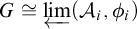 for some sequence
$(\mathcal {A}_i,\phi _i)_{i\in {\mathbb {N}}}$
for some sequence
$(\mathcal {A}_i,\phi _i)_{i\in {\mathbb {N}}}$
 as above.
The t.d.l.c. groups that are pro-countable are precisely the SIN groups (where SIN stands for “small invariant neighbourhoods); see [Reference Wesolek56, Section 2.2].
Remark B.2. Let G be a closed subgroup of
$S_\infty $
 , let
${\langle {N_i}\rangle }_{i\in {\mathbb {N}}}$
, let
${\langle {N_i}\rangle }_{i\in {\mathbb {N}}}$
 be a descending sequence of open normal subgroups of G with trivial intersection, and let
$\mathcal {A}_i= G/N_i$
be a descending sequence of open normal subgroups of G with trivial intersection, and let
$\mathcal {A}_i= G/N_i$
 . Then
$G \cong \varprojlim _{i>0} (\mathcal {A}_{i},\phi _i)$
. Then
$G \cong \varprojlim _{i>0} (\mathcal {A}_{i},\phi _i)$
 where the
$\phi _i$
where the
$\phi _i$
 are the canonical maps. This is well-known (see [Reference Malicki28, Lemma 2]).
B.2 Computably procountable groups.
Extending Definition 7.2 of computable profinite presentations, (2) below allows the
$\mathcal {A}_i$
 to be discrete computable groups, while retaining the condition that the kernels of the connecting maps be finite and given by strong indices.
Definition B.3 [Reference Lupini, Melnikov and Nies26, Definition 3.4].
-
(1) A computable presentation of a procountable group G is a sequence $(\mathcal {A}_{i},\phi _i)_{ i \in {\mathbb {N}}}$
of discrete groups
$\mathcal {A}_i$
and epimorphisms
$\phi _i: \mathcal {A}_{i} \rightarrow \mathcal {A}_{i-1} $
(for
$i>0$
) such that
$G\cong \varprojlim (\mathcal {A}_{i},\phi _i)$
, each group
$\mathcal {A}_i $
is uniformly computable as a discrete group, and the sequence of maps
$(\phi _i)_{ i \in {\mathbb {N}}^+}$
is uniformly computable. -
(2) Suppose that $ {ker\ } \phi _i$
is finite for each i, so that G is locally compact by [Reference Lupini, Melnikov and Nies26, Fact 3.2]. We say that
$(\mathcal {A}_{i},\phi _i)_{ i \in {\mathbb {N}}}$
is a computably procountable presentation with effectively finite kernels if in addition, from i one can compute a strong index for
$ {ker\ } \phi _i$
as a subset of
$A_i$
.





Fact B.4. If G is compact and has a computable procountable presentation with effectively finite kernels, then this presentation is a computable profinite presentation.
Proof. Since G is compact, the
$\mathcal {A}_i$
 are finite. All we need is strong indices for the
$\mathcal {A}_i$
are finite. All we need is strong indices for the
$\mathcal {A}_i$
 as groups. Since the
$\mathcal {A}_i$
as groups. Since the
$\mathcal {A}_i$
 are computable groups uniformly in i, it suffices to compute the size
$|\mathcal {A}_i|$
are computable groups uniformly in i, it suffices to compute the size
$|\mathcal {A}_i|$
 uniformly in i. One can do this recursively, using that
$|\mathcal {A}_i| = | {ker}\, \phi _i | \times |\mathcal {A}_{i-1}|$
uniformly in i. One can do this recursively, using that
$|\mathcal {A}_i| = | {ker}\, \phi _i | \times |\mathcal {A}_{i-1}|$
 .
.
Proposition B.5. If a t.d.l.c. group G has a procountable presentation
$(\mathcal {A}_{i},\phi _i)_{ i \in {\mathbb {N}}}$
 with effectively finite kernels, then G has a computable Baire presentation.
Proof. This is a straightforward extension of the argument in the profinite setting (Proposition 7.3). For simplicity we may assume that
$\mathcal {A}_0$
 is infinite. So we can effectively identify the elements of
$\mathcal {A}_i$
is infinite. So we can effectively identify the elements of
$\mathcal {A}_i$
 with
${\mathbb {N}}$
with
${\mathbb {N}}$
 , and hence view
$\phi _i $
, and hence view
$\phi _i $
 as a map
${\mathbb {N}} \to {\mathbb {N}}$
as a map
${\mathbb {N}} \to {\mathbb {N}}$
 . As before,

It is clear from the hypotheses that
$[\sigma ]_T$
 is compact iff
$\sigma $
is compact iff
$\sigma $
 is a nonempty string, and hence that T is computably locally compact via
$k=1$
is a nonempty string, and hence that T is computably locally compact via
$k=1$
 . The rest is as before, using that the
$\mathcal {A}_i$
. The rest is as before, using that the
$\mathcal {A}_i$
 are computable groups uniformly in i.
For abelian, as well as for compact, t.d.l.c. groups, we can provide a converse to the foregoing observation. The compact case essentially restates [Reference Smith52, Theorem 1] for the recursively profinite case.
Proposition B.6. Let G be an infinite computably t.d.l.c. group that is abelian or compact. Then G has a computably procountable presentation with effectively finite kernels.
Proof. Suppose that the meet groupoid
$\mathcal {W}(G)$
 has a Haar computable copy
$\mathcal {W}$
has a Haar computable copy
$\mathcal {W}$
 as in Definition 4.6. We may assume that its domain is all of
${\mathbb {N}}$
as in Definition 4.6. We may assume that its domain is all of
${\mathbb {N}}$
 , and that
$0$
, and that
$0$
 denotes a (compact open) subgroup. In the framework of that copy one can compute a descending sequence
${\langle {U_i}\rangle }_{i\in {\mathbb {N}}}$
denotes a (compact open) subgroup. In the framework of that copy one can compute a descending sequence
${\langle {U_i}\rangle }_{i\in {\mathbb {N}}}$
 of compact open subgroups of G, such that
$U_0$
of compact open subgroups of G, such that
$U_0$
 is the group denoted by
$0$
is the group denoted by
$0$
 and, for each compact open U, there is an i with
$U_i \subseteq U$
and, for each compact open U, there is an i with
$U_i \subseteq U$
 . In the abelian case, trivially each
$U_i$
. In the abelian case, trivially each
$U_i$
 is normal; in the case that G is compact, we effectively shrink the
$U_i$
is normal; in the case that G is compact, we effectively shrink the
$U_i$
 so that they are also normal. To do so, by the hypothesis that
$\mathcal {W}$
so that they are also normal. To do so, by the hypothesis that
$\mathcal {W}$
 is Haar computable, we can compute from i a strong index for the set
$\{B_1, \ldots , B_k\}$
is Haar computable, we can compute from i a strong index for the set
$\{B_1, \ldots , B_k\}$
 of distinct right cosets of
$U_i$
of distinct right cosets of
$U_i$
 ; now replace
$U_i$
; now replace
$U_i$
 by
$\bigcap _{r=1}^k B_r^{-1} \cdot U_i \cdot B_r$
by
$\bigcap _{r=1}^k B_r^{-1} \cdot U_i \cdot B_r$
 .
.
Let
$\mathcal {A}_i$
 be the automorphism group of the object
$U_i$
be the automorphism group of the object
$U_i$
 in the groupoid
$\mathcal {W}$
in the groupoid
$\mathcal {W}$
 viewed as a category; that is,
$\mathcal {A}_i$
viewed as a category; that is,
$\mathcal {A}_i$
 is the set of cosets of
$U_i$
is the set of cosets of
$U_i$
 , with the groupoid operations restricted to it. For
$i>0$
, with the groupoid operations restricted to it. For
$i>0$
 let
$\phi _i \colon \mathcal {A}_{i} \to \mathcal {A}_{i-1}$
let
$\phi _i \colon \mathcal {A}_{i} \to \mathcal {A}_{i-1}$
 be the map sending
$B \in \mathcal {A}_i$
be the map sending
$B \in \mathcal {A}_i$
 to the unique coset of
$U_{i-1}$
to the unique coset of
$U_{i-1}$
 that contains B. Since
$\mathcal {W}$
that contains B. Since
$\mathcal {W}$
 is Haar computable, the condition in (1) of Definition B.3 holds. Also, the kernel of
$\phi _i$
is Haar computable, the condition in (1) of Definition B.3 holds. Also, the kernel of
$\phi _i$
 is the set of cosets of
$U_i$
is the set of cosets of
$U_i$
 contained in
$U_{i-1}$
contained in
$U_{i-1}$
 . By Definition 4.6(b) we can compute the number of such cosets, so we can compute a strong index for the kernel. Hence the condition in (2) of Definition B.3 also holds.
We complete the proof by verifying the following claim.
Claim B.7.
$G \cong \varprojlim _{i>0} (\mathcal {A}_{i},\phi _i)$
 .
.
As in Definition 5.2, let
$\widetilde G $
 be the closed subgroup of
$ S_\infty $
be the closed subgroup of
$ S_\infty $
 of elements p that preserve the inclusion relation on
$\mathcal {W}$
of elements p that preserve the inclusion relation on
$\mathcal {W}$
 in both directions, and satisfy
$p(A) \cdot B = p(A\cdot B) $
in both directions, and satisfy
$p(A) \cdot B = p(A\cdot B) $
 whenever
$A \cdot B$
whenever
$A \cdot B$
 is defined. Recall that
$\widetilde G \cong G$
is defined. Recall that
$\widetilde G \cong G$
 . So it suffices to show that
$\widetilde G \cong \varprojlim (\mathcal {A}_{i},\phi _i)$
. So it suffices to show that
$\widetilde G \cong \varprojlim (\mathcal {A}_{i},\phi _i)$
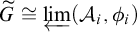 .
.
Let
$\mathcal {N}_i$
 be the stabilizer of
$U_i$
be the stabilizer of
$U_i$
 , which is a compact open subgroup of
$\widetilde G$
, which is a compact open subgroup of
$\widetilde G$
 . Since each
$p\in \widetilde G$
. Since each
$p\in \widetilde G$
 preserves the inclusion relation, we have
$\mathcal {N}_i \subseteq \mathcal {N}_{i-1}$
preserves the inclusion relation, we have
$\mathcal {N}_i \subseteq \mathcal {N}_{i-1}$
 for
$i>0$
for
$i>0$
 . By the choice of the
$U_i$
. By the choice of the
$U_i$
 , the intersection of the
$\mathcal {N}_i$
, the intersection of the
$\mathcal {N}_i$
 is trivial. Each
$\mathcal {N}_i$
is trivial. Each
$\mathcal {N}_i$
 is normal: if
$p \in \mathcal {N}_i$
is normal: if
$p \in \mathcal {N}_i$
 and
$q \in \widetilde G$
and
$q \in \widetilde G$
 , let
$B= q(U_i)$
, let
$B= q(U_i)$
 , a left, and hence also right, coset of
$U_i$
, a left, and hence also right, coset of
$U_i$
 . Then

So
$q^{-1}pq \in \mathcal {N}_i$
 .
.
For each i, the map
$\widetilde G \to \mathcal {A}_i$
 sending p to
$p(U_i)$
sending p to
$p(U_i)$
 induces a group isomorphism
$\widetilde G / \mathcal {N}_i \to \mathcal {A}_i$
induces a group isomorphism
$\widetilde G / \mathcal {N}_i \to \mathcal {A}_i$
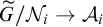 . For each
$i>0 $
. For each
$i>0 $
 the natural map
$\alpha _i \colon \widetilde G/\mathcal {N}_i \to \widetilde G/\mathcal {N}_{i-1}$
the natural map
$\alpha _i \colon \widetilde G/\mathcal {N}_i \to \widetilde G/\mathcal {N}_{i-1}$
 induced by the identity on
$\widetilde G$
induced by the identity on
$\widetilde G$
 corresponds to
$\phi _i$
corresponds to
$\phi _i$
 via these isomorphisms. Thus
$\varprojlim _{i>0} (\widetilde G/\mathcal {N}_{i},\alpha _i)\cong \varprojlim _{i>0} (\mathcal {A}_{i},\phi _i)$
via these isomorphisms. Thus
$\varprojlim _{i>0} (\widetilde G/\mathcal {N}_{i},\alpha _i)\cong \varprojlim _{i>0} (\mathcal {A}_{i},\phi _i)$
 . The claim now follows in view of Remark B.2.
Acknowledgments
The authors would like to thank Stephan Tornier and George Willis for very helpful discussions and insights.
Funding
A.M. was supported by the Rutherford Discovery Fellowship RDF-VUW1902 of the Royal Society Te Apārangi. A.N. was supported by the Royal Society Te Apārangi under the standard Marsden grant UOA-1931.


 Open access

