


1. Introduction
Life expectancy in Germany has increased substantially over the past decades. Focusing on West Germany, average remaining life expectancy at the age of 65 increased from 12.1 years in 1970–1972 to 17.8 years in 2020–2022 for men and from 15.2 years to 20.9 years for women (German Federal Statistical Office 2023). However, the likelihood of living a long life is not equal for all individuals and rather depends on their personal circumstances as there are clear mortality differentials by socioeconomic status (see, e.g., Haan et al., Reference Haan, Kemptner and Lüthen2020; Luy et al., Reference Luy, Wegner-Siegmundt, Wiedemann and Spijker2015; Von Gaudecker & Scholz Reference Von Gaudecker and Scholz2007) and across geographical areas (see, e.g., Kibele Reference Kibele2012; Rau & Schmertmann Reference Rau and Schmertmann2020; van Raalte et al., Reference van Raalte, Klüsener, Oksuzyan and Grigoriev2020).
Many studies from across the globe convincingly show that higher income is associated with a longer lifespan (e.g., Cutler et al., Reference Cutler, Deaton and Lleras-Muney2006; Dahl et al., Reference Dahl, Kreiner, Nielsen and Serena2024; Kinge et al., Reference Kinge, Modalsli, Øverland, Gjessing, Tollånes, Knudsen, Skirbekk, Strand, Håberg and Vollset2019). A growing body of recent studies, moreover, shows that it is not just an individual’s socioeconomic status that matters for when they die but also the place where they live (e.g., Chetty et al., Reference Chetty, Stepner, Abraham, Lin, Scuderi, Turner, Bergeron and Cutler2016; Deryugina & Molitor Reference Deryugina and Molitor2021; Finkelstein et al., Reference Finkelstein, Gentzkow and Williams2021). However, the interaction between an individual’s socioeconomic status and their place of residence in the context of their importance for life expectancy is only poorly understood to date. For example, only very limited evidence (Chetty et al., Reference Chetty, Stepner, Abraham, Lin, Scuderi, Turner, Bergeron and Cutler2016) exists on the degree to which the link between income and life expectancy varies between different geographical regions within a country. Furthermore, while a number of existing studies aim to identify place characteristics that are associated with longevity (e.g., Dwyer-Lindgren et al., Reference Dwyer-Lindgren, Bertozzi-Villa, Stubbs, Morozoff, Mackenbach, van Lenthe, Mokdad and Murray2017; Finkelstein et al., Reference Finkelstein, Gentzkow and Williams2021; Latzitis et al., Reference Latzitis, Sundmacher and Busse2011; Rau & Schmertmann Reference Rau and Schmertmann2020), there is a clear shortage of literature on the question of whether place health effects are heterogeneous for individuals of different socioeconomic status, as recently stressed by Deryugina and Molitor (Reference Deryugina and Molitor2021). In addition, to the best of my knowledge, no study to date investigates whether place health effects and their interaction with socioeconomic status change over time.
I contribute to these underexplored research topics in the following ways. Using administrative data from the German Pension Insurance, I estimate remaining life expectancy at age 65 by lifetime earnings quintileFootnote 1 and geographic area (NUTS2).Footnote 2 This allows me, for the first time for (West) Germany, to analyse regional differentials in life expectancy of individuals with similar (lifetime) earnings and consequently, to examine the degree of geographical and temporal variation in area-specific longevity gaps between individuals at the top and the bottom of the income distribution. Subsequently, I use these earnings – and region-specific life expectancy estimates together with a rich set of place characteristics obtained by combining different data sources (see Appendix B for an overview) to conduct a correlational analysis to investigate which place factors are associated with longevity. Specifically, I examine whether place matters differently for individuals’ life expectancy depending on their socioeconomic status and whether this interaction between place factors, socioeconomic status and life expectancy has changed over time. Due to data limitations (see Subsection 2.2), my analyses only focus on West German men.
I provide first evidence for substantial heterogeneity in the relationship between lifetime earnings and life expectancy across NUTS2 regions in West Germany. My results suggest a general trend of increasing area-specific longevity gaps over time. Furthermore, regional inequality in longevity gaps across different areas declined over time. Place factors associated with longevity are better healthcare supply, lower air pollution levels, lower regional poverty levels, and a higher prevalence of healthy behaviors (less smoking, lower obesity rates, higher exercise rates, and healthier diet). However, there is no clear evidence for heterogeneity in place factors associated with longevity by socioeconomic status: place characteristics do not seem to influence the longevity of individuals at the top and the bottom of the lifetime earnings distribution in different directions or magnitudes. Additionally, I find suggestive evidence for some weak time trends regarding place factors associated with longevity for individuals at the bottom of the lifetime earnings distribution but not for individuals at the top. It appears possible that place used to matter more in West Germany for individuals with low socioeconomic status but that over time the importance of place for their health has declined.
My study contributes to three strands of literature: first, the literature on mortality differentials by socioeconomic status and geographic area; second, the literature on place factors associated with longevity; and third, the literature on the heterogeneity of place health effects by socioeconomic status.
The study closest to mine is the paper by Chetty et al. (Reference Chetty, Stepner, Abraham, Lin, Scuderi, Turner, Bergeron and Cutler2016) which, to the best of my knowledge, is the only other study estimating life expectancy differentiated by income and region. They provide evidence for substantial regional variation in the relationship between socioeconomic status and life expectancy in the United States (U.S.). With the exception of Montez et al. (Reference Montez, Zajacova, Hayward, Woolf, Chapman and Beckfield2019) – who estimates life expectancy by educational level and region – other related existing studies either estimate life expectancy by different socioeconomic status but not by geographical area (e.g., Haan et al., Reference Haan, Kemptner and Lüthen2020; Kinge et al., Reference Kinge, Modalsli, Øverland, Gjessing, Tollånes, Knudsen, Skirbekk, Strand, Håberg and Vollset2019) or they calculate life expectancy estimates for different regions without differentiating between individuals of different socioeconomic status (e.g., Dwyer-Lindgren et al., Reference Dwyer-Lindgren, Bertozzi-Villa, Stubbs, Morozoff, Mackenbach, van Lenthe, Mokdad and Murray2017; Hrzic et al., Reference Hrzic, Vogt, Brand and Janssen2023; Rau & Schmertmann Reference Rau and Schmertmann2020). Studies on the relationship between income and life expectancy point toward an international trend of rising inequality in life expectancy by income (e.g., Cristia Reference Cristia2009; Dahl et al., Reference Dahl, Kreiner, Nielsen and Serena2024; van Raalte et al., Reference van Raalte, Sasson and Martikainen2018). For Germany, a small number of studies specifically find rising longevity differentials between individuals with high and low lifetime earnings using administrative data (e.g., Haan et al., Reference Haan, Kemptner and Lüthen2020; Kibele et al., Reference Kibele, Jasilionis and Shkolnikov2013; Wenau et al., Reference Wenau, Grigoriev and Shkolnikov2019). Furthermore, a number of studies for different countries show evidence for varying life expectancies across regions, for example Dwyer-Lindgren et al. (Reference Dwyer-Lindgren, Bertozzi-Villa, Stubbs, Morozoff, Mackenbach, van Lenthe, Mokdad and Murray2017) for the U.S., Rashid et al. (Reference Rashid, Bennett, Paciorek, Doyle, Pearson-Stuttard, Flaxman, Fecht, Toledano, Li, Daby, Johnson, Davies and Ezzati2021) for the U.K., Bonnet and d’Albis (Reference Bonnet and d’Albis2020) for France and Janssen et al. (Reference Janssen, Van den Hende, De Beer and van Wissen2016) for the Netherlands. Several existing studies for Germany provide evidence for mortality differentials across districts (e.g., Kibele Reference Kibele2012; Kibele et al., Reference Kibele, Klüsener and Scholz2015; Latzitis et al., Reference Latzitis, Sundmacher and Busse2011; Rau & Schmertmann Reference Rau and Schmertmann2020). Additionally, van Raalte et al. (Reference van Raalte, Klüsener, Oksuzyan and Grigoriev2020) and Redler et al. (Reference Redler, Wuppermann, Winter, Schwandt and Currie2021) provide evidence for decreasing regional variation in mortality in Germany over time. van Raalte et al. (Reference van Raalte, Klüsener, Oksuzyan and Grigoriev2020) also show that regional inequality in life expectancy in Germany is relatively low compared to other countries such as the U.S., the U.K., or France.
A number of previous studies for Germany examine the link between regional characteristics and longevity (e.g., Hrzic et al., Reference Hrzic, Vogt, Brand and Janssen2023; Kibele Reference Kibele2012; Latzitis et al., Reference Latzitis, Sundmacher and Busse2011; Rau & Schmertmann Reference Rau and Schmertmann2020). Place factors in these existing studies mainly consist of healthcare indicators (e.g., number of physicians, hospital density), economic indicators (e.g., unemployment rate and average household income), and social conditions (e.g., share of welfare recipients, education, and voter turnout). I expand on these analyses by further including direct measures for regional inequality, air pollution and health-related behaviors which have emerged as the standard in recent cutting-edge studies for the U.S. (Chetty et al., Reference Chetty, Stepner, Abraham, Lin, Scuderi, Turner, Bergeron and Cutler2016; Dwyer-Lindgren et al., Reference Dwyer-Lindgren, Bertozzi-Villa, Stubbs, Morozoff, Mackenbach, van Lenthe, Mokdad and Murray2017; Deryugina & Molitor Reference Deryugina and Molitor2021; Finkelstein et al., Reference Finkelstein, Gentzkow and Williams2021).
Generally, studies on the heterogeneity of place factors associated with longevity by socioeconomic status are scarce. For Germany, only two studies to date have touched on this topic in a noncomprehensive manner. Both Kibele (Reference Kibele2012) and Kibele (Reference Kibele2014) find some evidence that the mortality risk of high-income individuals is less affected by regional effects than it is the case for individuals at the bottom of the income distribution. However, in contrast to my study, these two papers only analyse one single regional factor Kibele (Reference Kibele2012) or summarize regional characteristics into one deprivation index Kibele (Reference Kibele2012). The few more closely related recent studies focus primarily on the U.S. (Chetty et al., Reference Chetty, Stepner, Abraham, Lin, Scuderi, Turner, Bergeron and Cutler2016; Finkelstein et al., Reference Finkelstein, Gentzkow and Williams2021; Montez et al., Reference Montez, Zajacova, Hayward, Woolf, Chapman and Beckfield2019) and find that geographic variation in life expectancy or mortality risk is higher for individuals of lower socioeconomic status, suggesting that place matters more for this group. According to Chetty et al. (Reference Chetty, Stepner, Abraham, Lin, Scuderi, Turner, Bergeron and Cutler2016), correlations between regional life expectancy and some place characteristics (e.g., access to healthcare) are significantly different between high-income and low-income individuals.
The paper is structured as follows: Section 2 describes the institutional setting and the data. In Section 3, I explain the methodological approach for estimating period – and region-specific life expectancy. Section 4 first presents evidence for heterogeneity in life expectancy differentiated by lifetime earnings across NUTS2 regions in West Germany and then investigates whether place matters differently for individuals’ life expectancy depending on their socioeconomic status and whether this interaction between place factors, socioeconomic status and life expectancy changed over time. Section 5 offers a discussion of the results. Section 6 concludes the paper.
2. Institutional setting and data
2.1. The German public pension system
Since pension entitlements are subsequently used as a proxy for lifetime earnings, this subsection provides a brief overview over the key characteristics of the German public pension system.Footnote 3
Most employees in Germany are mandatorily covered by the German Public Pension System, which is a pay-as-you-go system.Footnote 4 Over their career, individuals contribute a certain percentage of their annual gross earnings to accumulate pension entitlements which are called “earnings points.” Earnings points essentially refer to an individual’s relative position in the annual earnings distribution: if an individual’s annual earnings are equal to the average annual earnings, then they earn exactly one earnings point for this specific year. If they earn 50% more than the average annual earnings, they acquire 1.5 earnings points. 50% less than the average annual earnings will bring them 0.5 earnings points. However, maximum annual pension contributions are capped at around twice the amount of average annual earnings, which means that an individual can only earn a maximum of around two earnings points in a single year.Footnote 5 After accumulating earnings points over their work life, retired individuals receive gross monthly pension payments which are equal to their number of accrued earnings point multiplied with the applicable pension value.Footnote 6 There are some options for early retirement before the regular retirement age of 65 for individuals of birth cohorts included in my study; however, in general, pension payments are proportional to pension contributions over the life-cycle.Footnote 7 This means that accumulated pension entitlements are directly related to individual earnings over the life cycle and are therefore a commonly used proxy for lifetime earnings (see e.g., Haan et al., Reference Haan, Kemptner and Lüthen2020; Wenau et al., Reference Wenau, Grigoriev and Shkolnikov2019).
2.2. Pension data
Information on lifetime earnings and mortality was obtained from high-quality administrative data provided by the German Pension Insurance. Specifically, I use the SK90 dataset covering all mandatorily covered German pensioners, which is available for the calendar years 1992–2015. This dataset contains yearly information on pensioners’ age, sex, current place of residence (NUTS2), individual pension entitlements, and year of death.Footnote 8 I focus on life expectancy at age 65 and only include individuals aged 65 years or over for two reasons: comparability to other studiesFootnote 9 and avoiding selection problems resulting from varying retirement ages, for example, in the case of the early retirement of disabled individuals. At age 65, this potential selection problem does not occur since nearly all individuals are retired.Footnote 10 The restricted dataset includes individuals born between 1905 and 1949.
Similarly to related earlier studies (e.g., Kibele et al., Reference Kibele, Jasilionis and Shkolnikov2013; Von Gaudecker & Scholz, Reference Von Gaudecker and Scholz2007; Wenau et al., Reference Wenau, Grigoriev and Shkolnikov2019), I solely focus on men. Unfortunately, the data do not allow for the investigation of the relationship between lifetime earnings and mortality for women. This is mainly the due to institutional reasons as, until 1967, women were legally allowed to leave the pension system when they married and collect the monetary value of their accumulated pension entitlements. Until 1995, they were able to re-join the pension system at a later point in life with the help of retroactive payments of contribution. In such cases, women´s pension entitlements are no longer closely related to their employment biographies and lifetime earnings. Furthermore, the SK90 dataset do not contain information on whether women re-entered the pension system or not. Additionally, because of the low female labor market participation rates for the cohorts analysed in this study, female earnings points in general do not adequately reflect women’s socioeconomic status and their life chances.
Moreover, in my main analysis, I focus on West German men only. The reason for this limitation is that East Germans aged 65 years or over in the years between 1995 and 2015 spent large parts of their working lives in the German Democratic Republic (GDR), meaning their earnings information, wage levels, and therefore, earnings points are not easily comparable to those of individuals from the same birth cohorts who lived and worked in Federal Republic of Germany (FDR).Footnote 11 Furthermore, the data does not cover earnings information for periods of self-employment or civil service, meaning that complete earnings biographies and, as such, lifetime earnings of self-employed individuals and civil servants are not available. In order to address this problem and obtain a sample of individuals with complete earnings information, I follow the approach of related studies (e.g., Haan et al., Reference Haan, Kemptner and Lüthen2020; Von Gaudecker & Scholz, Reference Von Gaudecker and Scholz2007; Wenau et al., Reference Wenau, Grigoriev and Shkolnikov2019) and restrict the sample to individuals who accumulated at least 30 earnings points up to the age of 65. As a consequence, I automatically also drop individuals with very low lifetime earnings, which likely leads to a slight underestimation of the heterogeneity in life expectancy by lifetime earnings.Footnote 12
In total, the restricted dataset offers around 65.04 million person-year observations for West German men. Among them are 3.31 million (5.09%) observed deaths.
3. Methodology
Methodologically, I closely follow the approach of Haan et al. (Reference Haan, Kemptner and Lüthen2020) to estimate the remaining life expectancy at age 65 for West German men using pension data. This provides a well-established framework for deriving life expectancy measures from German pension data. However, my study has two key differences from their approach. First, I conduct the analysis on a regional level (NUTS2), which allows for the examination of spatial differences in the link between lifetime earnings and life expectancy.Footnote 13 And second, I estimate and analyse period life expectancy instead of cohort life expectancy. In contrast to cohort life expectancy, which uses information on mortality of the same cohort over time, period life expectancy makes use of mortality of different cohorts in a given year or period. The life expectancy measure used in this study – remaining period life expectancy at age 65 – therefore refers to the average length of life left for a hypothetical individual aged 65 experiencing age-mortality rates for the rest of their life equal to those in the cross-section in a given period. Period life expectancy is frequently used in recent studies on trends in inequality in longevity (e.g., Chetty et al., Reference Chetty, Stepner, Abraham, Lin, Scuderi, Turner, Bergeron and Cutler2016; Currie & Schwandt, Reference Currie and Schwandt2016; Dahl et al., Reference Dahl, Kreiner, Nielsen and Serena2024; Kinge et al., Reference Kinge, Modalsli, Øverland, Gjessing, Tollånes, Knudsen, Skirbekk, Strand, Håberg and Vollset2019;) and allows for matching with yearly data on a variety of regional indicators (see Subsection 4.2).
Individuals are assigned to lifetime earnings quintiles based on their accumulated earnings points relative to all other West German male pensioners of the same five-year age group (seven age groups from age 65–69 to age 95–99) in each calendar year.Footnote 14 To ensure a sufficient number of observations in less-populated NUTS2 regions, I group the person-year observations for the years 1992–2015 into eight three-year time periods as I estimate period life expectancy for time periods instead of single years.Footnote 15 I use observations for the time periods 1992–1994 and 1995–1997 for the estimation to increase precision of the age-mortality rates estimates. However, since I do not have access to many of the regional indicators for Subsection 4.2 (e.g., healthcare supply indicators) for the years before 1998, I do not estimate and report mortality rates and consequently life expectancy for these time periods.
I calculate life expectancies using a standard two-step approach. First, I estimate period – and region-specific conditional age-mortality rates by lifetime earnings quintiles for all the ages between 65 and 99. Next, these age-mortality rates are the basis for constructing life tables and deriving earnings – and period-specific life expectancy at the age of 65 at NUTS2 level.
The probability of death within the next year is estimated using a logistic regression model accounting for heterogeneous age effects which may differ by lifetime earnings quintiles. I allow for region-specific effects of age, periods and earnings as well as their interactions. Additionally, I control for regional period-specific fixed effects ( ${\mu _{rt}}$
), regional-specific lifetime earnings fixed effects (
${\mu _{rt}}$
), regional-specific lifetime earnings fixed effects ( ${\eta _{rq}}$
), and the fixed effects of period-earnings interactions (
${\eta _{rq}}$
), and the fixed effects of period-earnings interactions ( ${\nu _{rtq}}$
). The respective log-odds can be expressed as follows:
${\nu _{rtq}}$
). The respective log-odds can be expressed as follows:
 $$\begin{align}log{{(Pr(deat{h_{iatqr}}|survival\,until\,age\,a)} \over {1 - Pr(deat{h_{iatqr}}|survival\,until\,age\,a)}} = &{\beta _0} + \sum_{p = 1}^4 {{\beta _{rp}}\,{a^p}} \\&+ \sum_{p = 1}^4 {{\beta _{rpq}}\,{a^p} + {\mu _{rt}} + {\eta _{rq}} + {\nu _{rtq}}} \end{align}$$
with q refering to individuals’i lifetime earnings quintile of time period t and a to the age of the respective individual from region r.Footnote 16
In the next step, I use the parameter estimates to predict conditional age-specific mortality rates. Finally, I calculate for every NUTS2 region separately remaining life expectancy at age 65 by periods and lifetime earnings quintiles using the following formula:
 $$\sum_{z = 65}^{99} {\Pi _{a = 65}^z[1 - Pr(deat{h_{atqr}})]} $$
where $Pr\left( {dat{h_{atqr}}} \right)$
is the region-specific age-mortality rate for period t and lifetime earnings quintile q. This approach follows the underlying assumption that individuals’ maximum age is 100 and therefore their probability of death at age 100 is equal to 1.
$Pr\left( {dat{h_{atqr}}} \right)$
is the region-specific age-mortality rate for period t and lifetime earnings quintile q. This approach follows the underlying assumption that individuals’ maximum age is 100 and therefore their probability of death at age 100 is equal to 1.
As depicted by Figure A.2, the generated NUTS2 level life expectancy estimates (averaged across quintiles) are very highly correlated (r = 0.96) with life expectancy from external data provided by the European Statistical Office (Eurostat). I conclude from this external validation that my region – and quintile-specific life expectancy estimates are a valid and reliable measure for mortality of West German men at NUTS2 level.
4. Results
This section provides the main results of my analysis. It is divided into three parts. In Subsection 4.1, I investigate geographical variation and time trends of NUTS2-level life expectancy estimates. In Subsection 4.2, conducting a correlation analysis, I then analyse whether place matters differently for individuals’ life expectancy depending on their socioeconomic status and whether this interaction between place factors, socioeconomic status and life expectancy changed over time. Finally, in Subsection 4.3, I further examine the robustness of my heterogeneity analysis using a regression and slope testing approach.
4.1. Regional analysis
4.1.1. NUTS2-level variation in the link between lifetime earnings and life expectancy (2013–2015)
There exists substantial heterogeneity in the relationship between lifetime earnings and life expectancy across regions in West Germany. Focusing on the time period 2013–2015, Figure 1 (Subfigure 1) depicts life expectancy at age 65 both at the top and the bottom of the lifetime earnings distribution for the 30 West German NUTS2 regions. Life expectancy at the bottom of the distribution varied between 13.9 years in Saarland and 15.9 years in Tübingen.Footnote 17 Among top lifetime earners, individuals in Bremen had the lowest life expectancy (18.5 years) while in Trier they were expected to live for around 20.7 additional years. Across all regions, the (population-weighted) standard deviation of life expectancy was 0.52 years for men at the bottom of the distribution versus 0.55 years for men in the top lifetime earnings quintile. This finding of a roughly equal variation across different regions in life expectancy for individuals in the bottom and top quintile is robust for all time periods apart from the years 1998–2000 where the variation is higher for individuals at the bottom of the lifetime earnings distribution. Another striking result is that there is a strong correlation (r = 0.79) between the life expectancy of lifetime low earners and lifetime high earners in the same region and period of time.
Life expectancy (by quintiles) and the longevity gap by NUTS2 regions, 2013–2015 and change over time.
Notes: (1) Life expectancy by quintiles and NUTS2 regions, 2013–2015. Life expectancy in remaining years at age 65; (2) change in life expectancy by quintiles and NUTS2 regions, 1998–2000 vs. 2013–2015. The change in life expectancy refers to the absolute change (in years) between the periods 1998–2000 and 2013–2015; (3) longevity gap by NUTS2 regions, 2013–2015. The longevity gap refers to the difference in life expectancy between individuals in the 1st and 5th quintiles of the respective NUTS2 region; and (4) change in the longevity gap by NUTS2 regions, 1998–2000 vs. 2013–2015. The change in the longevity gap refers to the absolute change (in years) between the periods 1998–2000 and 2013–2015.
Source: Own calculations based on SK90 data.

Furthermore, Figure 1 (Subfigure 1) suggests regional clustering of NUTS2 regions with regards to individuals’ life expectancy by lifetime earnings. Four out of the eight NUTS2 regions with the lowest life expectancy for individuals in the 1st lifetime earnings quintile were clustered in the federal state of North Rhine-Westphalia, where as the NUTS2 regions with the highest life expectancy for low-income individuals were located in Baden-Württemberg (three of the top five). Clustering for individuals in the top quintile looks fairly similar, with life expectancies within North Rhine-Westphalia ranking among the lowest while top lifetime earners in the federal states of Baden-Württemberg and Bavaria on average live longest (seven of the top ten regions are clustered in these two federal states). At the same time, my results show that life expectancies both at the top and the bottom of the lifetime earnings distribution can also vary substantially for NUTS2 regions within the same federal state. For example, in Bavaria, life expectancy varies between 19.5 years in Upper Palatinate (“Oberpfalz”) and 20.3 years in Upper Bavaria (“Oberbayern”) at the top and 14.6 years in Central Franconia (“Mittelfranken”) and 15.8 years in Upper Bavaria at the bottom of the lifetime earnings distribution. In general, regions in the south of Germany tend to have higher life expectancies than regions in the north.
As depicted by Figure 1 (Subfigure 3), there is substantial regional variation in life expectancy differences between individuals in the 1st and the 5th lifetime earnings quintile. This longevity gap ranges from 4.1 years in Münster to 5.6 years in Trier and Upper Franconia (“Oberfranken”) with a (population-weighted) standard deviation of 0.35 years. These results provide evidence for a substantial regional heterogeneity in the extent to which differences in individuals’ socioeconomic status lead to different life expectancies.
4.1.2. Changes over time
There is an overall trend of rising average life expectancy for West German men over time, as Figure 2 shows. However, average life expectancy increased at different rates across the lifetime earnings distribution. Over the span of around 15 years, average improvements in absolute life expectancy were 1.8 years for the lifetime earnings poor (from 13.0 years to 14.8 years) and therefore lower than the increase of 2.7 years for the top lifetime earners (from 16.8 years to 19.5 years). As a result, the gap in average life expectancy between the bottom and top lifetime earnings quintile of West German male pensioners increased by 24% from 3.8 years in 1998–2000 to 4.7 years in the period 2013–2015.
Life expectancy of West German men by periods and quintiles.
Notes: Life expectancy in remaining years at age 65. Gray areas indicate 95% confidence intervals estimated using the Delta method.
Source: Own calculations based on SK90 data.

However, there is geographic variation in life expectancy trends over time. Figure 1 (Subfigure 2) maps the absolute change in life expectancy between the two time periods 1998–2000 and 2013–2015 by NUTS2 region for individuals at the top and bottom of the lifetime earnings distribution. Temporal trends in life expectancy varied more strongly in the 1st quintile (population-weighted standard deviation of 0.53), ranging between an increase of 0.96 years in Trier and 3.1 years in Münster.Footnote 18 Life expectancy improvements of top lifetime earners ranged between 2.1 years in Bremen and 3.4 years in Upper Palatinate, with a standard deviation of 0.25 years.
Similar to the national level (Figure 2), most NUTS2 regions follow the trend of increasing longevity gaps between individuals at the top and the bottom of the lifetime earnings distribution over time. In fact, this trend can be found for 29 of 30 NUTS2 regions in West Germany (Figure 1, Subfigure 4). The only exemption was Münster – the region with the highest increase in life expectancy for the bottom quintile – where the longevity gap decreased by 0.7 years. Among the 29 NUTS2 regions which experienced an increasing gap, the extent to which life expectancy between the lifetime earnings poor and rich diverged varied drastically across NUTS2 regions between 0.1 years in Arnsberg and 2.4 years in Upper Palatinate. Gaps in life expectancy between the bottom and top quintiles only increased slightly in regions in which individuals in the bottom quintile experienced the largest improvements in life expectancy. In contrast, regions which ranked highest regarding the life expectancy improvements for individuals in the top quintile tended to experience a strong increase in the longevity gap between the lifetime earnings poor and rich.Footnote 19 These temporal trends in NUTS2-level longevity gaps resulted in a decline in variation of those gaps across German NUTS2 regions over time. Specifically, the standard deviation decreased from 0.51 years in the period 1998–2000 to 0.35 years in 2013–2015.
4.2. Place factors associated with longevity
The results in Subsection 4.1 provide evidence for substantial heterogeneity in the relationship between lifetime earnings and life expectancy and how this relationship changed over time across NUTS2 regions in West Germany. Against this background, my aim in this section is to identify factors related to this regional variation in the association between life expectancy and lifetime earnings and make an important contribution to our understanding of the heterogeneity of place factors associated with longevity for individuals of different socioeconomic status and how this interaction changed over time.
As pointed out by two recent influential studies (Deryugina & Molitor Reference Deryugina and Molitor2021; Finkelstein et al., Reference Finkelstein, Gentzkow and Williams2021), several empirical challenges exist for the identification of causal effects of the place of residence on longevity. One such challenge is, for example, nonrandom sorting of high-income individuals into areas with attractive living conditions like high-quality and quantity supply of healthcare or low pollution. As a result, it is no longer clear whether comparably high average longevity in such areas is a direct effect of favorable place characteristics or just the result of a high number of healthy, high-income individuals. Furthermore, non-random sorting itself can be the source of place effects due to peer influence on health-related behaviors, leading to regional differences in life expectancy as a result of both non-random sorting and the peer influences of individuals who live in this region. Other empirical challenges are due to potential unobserved confounders and reverse causality.
Finkelstein et al. (Reference Finkelstein, Gentzkow and Williams2021) only very recently presented the first empirical approach which is convincingly able to isolate the causal impacts of place characteristics on life expectancy by making use of a quasi-experimental design where they analyse movers coming from the same place who end up in different locations. However, following their approach with administrative data from the German Pension Insurance is not feasible. Due to strict data protection guidelines, it is not possible to follow individuals over time and therefore no panel structure is available that would allow for an investigation of whether individuals moved to another region. Instead, I follow Chetty et al. (Reference Chetty, Stepner, Abraham, Lin, Scuderi, Turner, Bergeron and Cutler2016) in their approach of conducting bivariate correlational analysis. As a result, my results cannot be interpreted as causal, but are rather of suggestive and descriptive nature. My main focus is to investigate the heterogeneity of place factors associated with life expectancy by socioeconomic status and whether the potential moderating influence of socioeconomic status for the link between life expectancy and place factors changed over time – two perspectives that so far have been vastly overlooked in the literature.
Following recent cutting-edge studies on the link between place characteristics and longevity (e.g., Chetty et al., Reference Chetty, Stepner, Abraham, Lin, Scuderi, Turner, Bergeron and Cutler2016; Deryugina & Molitor Reference Deryugina and Molitor2021; Finkelstein et al., Reference Finkelstein, Gentzkow and Williams2021), I focus on the following place characteristics: health behaviors, healthcare, environment, inequality and poverty. I combine multiple different data sources to generate a comprehensive dataset on regional characteristics at NUTS2 level for the periods 1998–2000 and 2013–2015. Detailed definitions, data sources, and summary statistics for these characteristics are provided in Appendix B.
Figure 3 shows correlations of NUTS2-level life expectancy estimates for the 1st and 5th quintiles of the lifetime earnings distribution with regional area characteristics. The aim is to understand which factors are associated with longevity and whether there are differences for individuals at the top and the bottom of the distribution. I find evidence that, on average, longevity tends to be higher in areas where healthier behaviors are more prevalent. Specifically, the share of smokers at NUTS2 level is significantly negatively correlated with life expectancy – for both individuals at the top and the bottom of the lifetime earnings distribution. A region’s obesity rate is also negatively correlated with regional life expectancy, although the correlation is only significant for low-income individuals. In addition, there is a strong positive and significant correlation (0.49) between regional exercise rates and the life expectancy of individuals with low lifetime earnings, while this correlation is somewhat smaller in size (0.37) and not statistically significant for individuals at the top of the distribution. Furthermore, a higher share of individuals following a healthy diet is positively correlated with longevity. In terms of regional healthcare supply, my results show a significant positive correlation for both general practitioner density and hospital density with life expectancy at age 65 for individuals in the 1st and 5th quintiles of the lifetime earnings distribution. Correlations for all ambulatory doctors per capita is positive but not significant. The correlation between life expectancy and the number of hospital beds per capita, however, does not have the expected sign: more hospital beds are associated with lower life expectancy. Interestingly, this correlation is also found by other studies (e.g., Deryugina & Molitor Reference Deryugina and Molitor2021; Finkelstein et al., Reference Finkelstein, Gentzkow and Williams2021) and hints at the limits of using correlational analysis when trying to identify place factors associated with longevity. In this case, for example, more hospital beds could be a response to poor health and therefore increased health care needs among residents. Furthermore, I find significant negative correlations between different types of air pollution and life expectancy. However, it does not seem to be the case that the impact for low-income individuals is significantly worse than for high-income individuals. Moreover, inequality was more negatively correlated for individuals in the top lifetime earnings quintile. Regional poverty indicators – namely, the number of individuals on housing subsidy and elderly support per 1,00,000 inhabitants – are negatively correlated with life expectancy for both individuals at the top and the bottom of the lifetime earnings distribution. I find evidence that GDP per capita is positively correlated with life expectancy. The correlation is higher and significantly positive for individuals at the bottom of the distribution while it is weaker and not statistically significant for the top lifetime earners. Other analysed factors (population density and population share of academics) are not significantly correlated with life expectancy. These findings are essentially robust across the lifetime earnings distribution (see Figure A.4). It is important to note that, due to the descriptive nature of my analysis, I do not analyse potential interactions between different place factors.
Correlations between life expectancy and place characteristics, 2013–2015.
Notes: Population-weighted Pearson correlations estimated between NUTS2 region place characteristics and remaining life expectancy at age 65. The error bars indicate 95% confidence intervals, which are based on standard errors clustered by NUTS2 region. Detailed definitions of all variables can be found in Appendix B.
Sources: Life expectancies are based on own calculations using the SK90 dataset. The sources of the different place characteristics are presented in Appendix B.

To explore whether these associations between place characteristics and life expectancy changed over time, I also analysed correlations for the period 1998–2000 (see Figure A.5). There are no substantial differences with respect to the direction of the correlations or the heterogeneity between individuals at the top and the bottom of the distribution. However, it is striking that for the place characteristics related the ambulatory care (general practitioner density and ambulatory doctors), the correlations decreased in magnitude over time – specifically for the bottom quintile. The same holds true for the air pollution characteristics. Furthermore, correlations with smoking and a region’s exercise rate are not significant in the period 1998–2000.
Finally, I also investigate correlations between changes in regional place characteristics and longevity gaps over time (Figure A.6). Of all the analysed indicators, only changes over time in regional general practitioner density and $N{O_2}$
air pollution are significantly correlated with trends in regional longevity gaps. However, again, no conclusion regarding the direction of causality can be drawn from these results.
$N{O_2}$
air pollution are significantly correlated with trends in regional longevity gaps. However, again, no conclusion regarding the direction of causality can be drawn from these results.
As a sensitivity check for my correlational approach, I have also conducted correlational analysis using NUTS2-level, age-specific mortality rates for the 1st and 5th quintiles of the lifetime earnings distribution instead of life expectancy. As depicted by Figure A.7–10, our findings remain robust when using mortality rates instead of life expectancy.Footnote 20
4.3. Robustness of heterogeneity analysis
In order to explore in further detail and verify the robustness of my heterogeneity analysis, I now present an alternative approach to look at the heterogeneity of place factors associated with longevity by socioeconomic status and potential changes over time. Following recent studies analyzing the link between mortality and regional inequality in income (e.g., Currie & Schwandt Reference Currie and Schwandt2016; Redler et al., Reference Redler, Wuppermann, Winter, Schwandt and Currie2021), I implement a simple approach of bivariate regression analysis combined with slope testing. However, instead of solely focusing on inequality in income across different areas, I analyse a number of different place characteristics. First, for each period (1998–2000 and 2013–2015), I group the 30 NUTS2 regions into deciles according to, for example, their number of general practitioners (“GPs”), with the 1st decile referring to the three regions with the lowest number of GPs and the 10th decile containing the three regions with the highest GP density. Then, I calculate population-weighted average life expectancy by deciles and plot the ranks against the rank-specific average life expectancy.
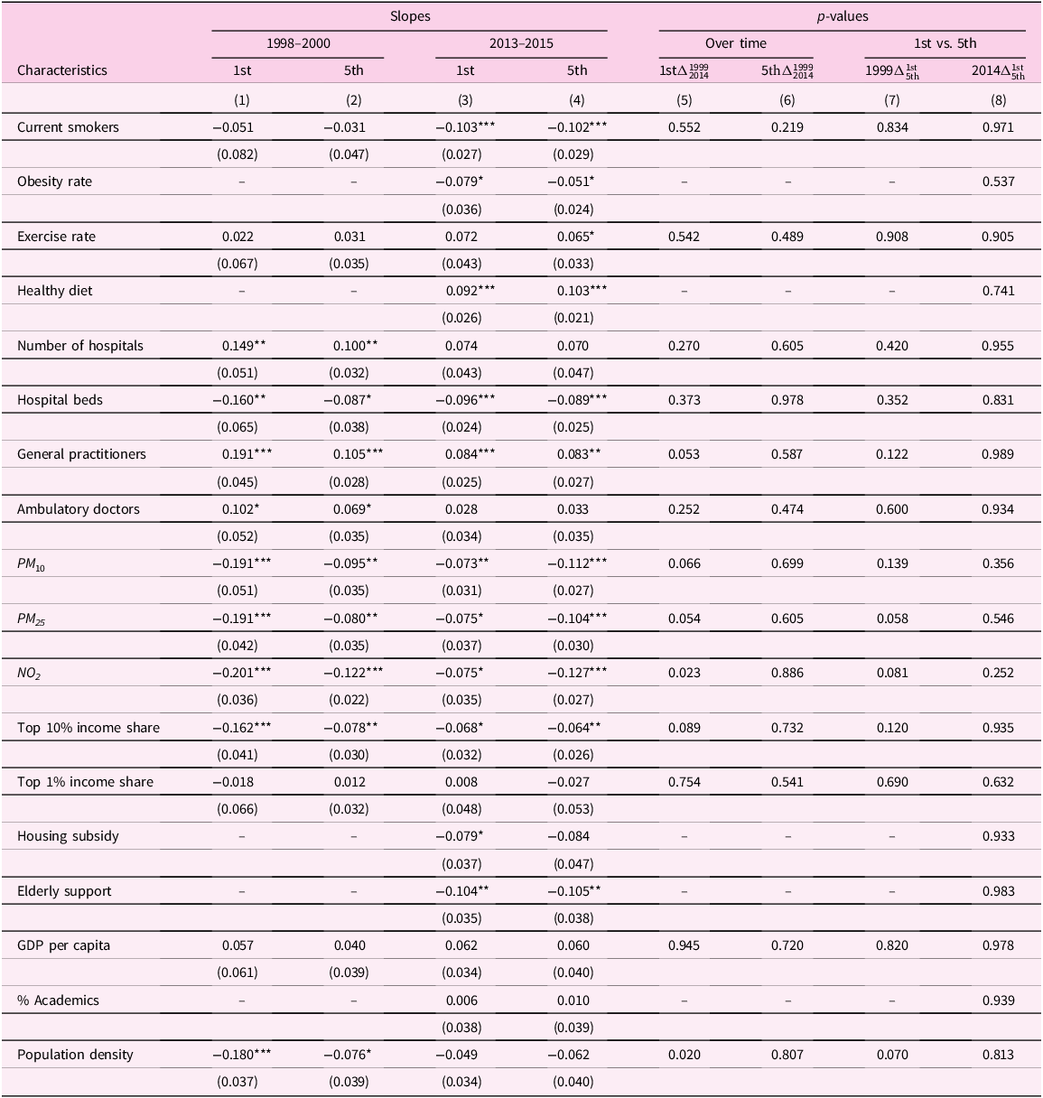
Exemplarily, Figure 4 depicts the results for the number of GPs per 100,000 inhabitants. Regions with a higher number of general practitioners have on average higher life expectancy estimates both for individuals at the top and the bottom of the lifetime earnings distribution in 1998–2000 and 2013–2015. Table 1 reports the slopes of the fitted regression lines (columns 1–4) and the p-values for the tests whether (1) slopes for the same quintile changed significantly over time (columns 5–6) and (2) slopes are significantly different for the 1st and 5th quintiles in the same period (columns 7–8). p-values higher than 0.05 mean that we cannot reject the null hypothesis of equal slopes, meaning that the association between a specific place characteristic and life expectancy for the 1st quintile did not significantly change over time or slopes between the 1st and 5th quintiles are not statistically different from each other suggesting no heterogeneity for individuals of different socioeconomic status.
Life expectancy and general practitioners per capita by quintiles and periods.
Notes: NUTS2 regions are grouped into deciles according to their number of general practitioners per capita. The gray areas around the fitted regression lines indicate the 95% confidence intervals.
Sources: Life expectancies are based on own calculations using the SK90 dataset. Information on the number of GPs per NUTS2 region was obtained from the National Association of Statutory Health Insurance Physicians (KBV).

Life expectancy and place characteristics – slopes of regression lines

Notes: Columns 1–4 report the slopes of the fitted regression lines for different periods and quintiles. Standard errors for regression coefficients are reported in parentheses. ***, ** and * denote significance at the 1, 5, and 10 percent levels, respectively. Columns 5–6 show the p-values for the null hypothesis that the quintile-specific slopes are equal in both periods. Columns 7–8 report the p-values for the null hypothesis that the slopes are equal for both quinitiles. Detailed definitions of all variables can be found in Appendix B.
Sources: Life expectancies are based on own calculations using the SK90 dataset. The sources of the different place characteristics are presented in Appendix B.
A closer look at the p-values for the slope test for whether the association between life expectancy and place characteristics changed over time (columns 5 and 6) shows that p-values are considerably lower for the bottom quintile. Moreover, for two place characteristics (NO 2 air pollution and population density), I can even reject the null hypothesis of equal slopes in 1998–2000 and 2013–2015. For both of these characteristics, the negative slope decreases significantly in magnitude over time. For other indicators (e.g., PM 10 and PM 25 air pollution and number of GPs), the p-values are very close to the 0.05 threshold. Consequently, my results suggest some evidence for time trends in place factors associated with longevity for individuals at the bottom of the lifetime earnings distribution. For individuals at the top of the distribution no evidence for time trends can be found (column 6). High p-values in columns 7 and 8 suggest that there is no significant heterogeneity in place factors associated with longevity between individuals at the top and the bottom of the lifetime earnings distribution. All in all, results from the slope testing approach are in line with the findings from the correlational analysis presented in Subsection Place factors associated with longevity.
5. Discussion
In line with prior studies (e.g., Von Gaudecker & Scholz, Reference Von Gaudecker and Scholz2007; Wenau et al., Reference Wenau, Grigoriev and Shkolnikov2019; Haan et al., Reference Haan, Kemptner and Lüthen2020), I find evidence for differences in life expectancy by lifetime earnings. However, one of the main contributions of this study is to present novel estimates of regional life expectancy at NUTS2 level for (West) Germany by lifetime earnings quintiles. Those estimates not only allow me to investigate inequality in life expectancy for individuals in the same lifetime earnings quintile across West German NUTS2 regions, but also longevity gaps for individuals within the same geographical area who are on different ends of the lifetime earnings distribution. My finding of increasing (region-specific) longevity gaps over time, driven primarily by large increases in top lifetime earners’ life expectancy, is consistent with the results for West German men by Haan et al. (Reference Haan, Kemptner and Lüthen2020), which do not differentiate by region. For the U.S., Chetty et al. (Reference Chetty, Stepner, Abraham, Lin, Scuderi, Turner, Bergeron and Cutler2016) also find similar results when analyzing the relationship between cross-sectional earnings and life expectancy. While recent studies by Dahl et al. (Reference Dahl, Kreiner, Nielsen and Serena2024) and Hagen et al. (Reference Hagen, Laun, Lucke and Palme2025) have advanced the understanding of potential drivers of the increasing longevity gap by socioeconomic status, the need for further research on this important topic remains. According to my results, while within-region longevity gaps are mostly rising, there is a decline in variation of those gaps across different NUTS2 regions over time. Other recent studies also show declining regional disparities in mortality rates (Redler et al., Reference Redler, Wuppermann, Winter, Schwandt and Currie2021) and life expectancy (van Raalte et al., Reference van Raalte, Klüsener, Oksuzyan and Grigoriev2020) across German regions.
The study by Chetty et al. (Reference Chetty, Stepner, Abraham, Lin, Scuderi, Turner, Bergeron and Cutler2016) for the U.S. is the only study to date that also analyses geographical variation in life expectancy differentiated by earnings. While it is important to note that methodological differences in factors such as earnings measures (cross-sectional household income vs. individual lifetime earnings), observation periods, age of analysed individuals, the area level of observation (30 German NUTS2 regions vs. 595 U.S. commuting zones), and differences in our divisions of the earnings distribution (quintiles vs. quartiles) hamper direct comparisons between my results and the findings presented by Chetty et al. (Reference Chetty, Stepner, Abraham, Lin, Scuderi, Turner, Bergeron and Cutler2016), some key similarities and differences become clear. Similarly to my results for West Germany, Chetty et al. (Reference Chetty, Stepner, Abraham, Lin, Scuderi, Turner, Bergeron and Cutler2016) find evidence for substantial variation in the relationship between socioeconomic status and life expectancy across U.S. geographical areas. Another similarity to my results for West Germany is that they present evidence for geographical clustering of regions with the highest and lowest life expectancies both at the bottom and the top of the lifetime earnings distribution in the U.S. Furthermore, they also find that in the U.S. not just levels of life expectancy, but also temporal trends vary significantly across regions. In contrast to my findings, however, Chetty et al. (Reference Chetty, Stepner, Abraham, Lin, Scuderi, Turner, Bergeron and Cutler2016) show that, in the U.S., life expectancy across all commuting zones varies more strongly among individuals in the bottom income quartile than for individuals in the top income quartile. In contrast, my results for West Germany show no difference in life expectancy variation between the 1st and 5th quintiles. Unfortunately, the abovementioned methodological differences between my study and the study by Chetty et al. (Reference Chetty, Stepner, Abraham, Lin, Scuderi, Turner, Bergeron and Cutler2016) make it very difficult to assess whether the finding by van Raalte et al. (Reference van Raalte, Klüsener, Oksuzyan and Grigoriev2020) that state-level inequality in overall life expectancy in the U.S. exceeds inequality in Germany also holds true when differentiating by (lifetime) earnings. It would be interesting to analyse more comprehensively how the regional variation I found for West Germany – which I assessed as being substantial – actually holds up in international comparisons. To answer this question, more studies for different countries are needed on the question to what extent life expectancy by socioeconomic status varies geographically.
In general, my findings on which regional characteristics are associated with longevity fit in well with previous findings for Germany. For example, existing studies for Germany (e.g., Kibele Reference Kibele2012; Latzitis et al., Reference Latzitis, Sundmacher and Busse2011; Rau & Schmertmann Reference Rau and Schmertmann2020; Redler et al., Reference Redler, Wuppermann, Winter, Schwandt and Currie2021) also provide evidence for an association between high mortality and regional deprivation indicators (e.g., unemployment rate and share of welfare beneficiaries). Previous findings regarding the role of regional healthcare supply indicators for longevity are rather inconclusive. Latzitis et al. (Reference Latzitis, Sundmacher and Busse2011) and Rau and Schmertmann (Reference Rau and Schmertmann2020), for example, find no clear association between regional life expectancy and the number of physicians per 100,000 inhabitants. However, this discrepancy between their results and mine could potentially be due to differences in the studies’ designs.Footnote 21 Furthermore, the significant negative correlations I find between the prevalence of unhealthy behaviors and life expectancy are in line with existing studies showing a negative effect of lifestyle risk factors (smoking, drinking, and obesity) on health and life expectancy in Germany (e.g., Janssen et al., Reference Janssen, Trias-Llimos and Kunst2021; Li et al., Reference Li, Hüsing and Kaaks2014). Similarly, the significant negative correlation between a NUTS2 region’s level of air pollution and regional life expectancy in Germany is not surprising given the well-established harmful effects of air pollution on population health found by earlier studies (e.g., Cohen et al., Reference Cohen, Brauer, Burnett, Anderson, Frostad, Estep, Balakrishnan, Brunekreef, Dandona, Dandona, Feigin, Freedman, Hubbell, Jobling, Kan, Knibbs, Liu, Martin, Morawska, Pope, Shin, Straif, Shaddick, Thomas, van Dingenen, van Donkelaar, Vos, Murray and Forouzanfar2017; Margaryan Reference Margaryan2021; Pestel & Wozny Reference Pestel and Wozny2021).
However, a limitation of my study is that the administrative dataset used only offers information on the current place of residence for individuals aged 65 years or older, but no information on where people used to live in the past and on the time of relocation. Thus, I cannot rule out the possibility that some individuals spent a large part of their lives living in different regions (where they were exposed to different place health effects) from the ones I can attribute to them. For example, a number of existing studies show that children growing up in more deprived areas end up to having worse health outcomes as adults compared with individuals who grew up in better-off communities (e.g., Hayward & Gorman Reference Hayward and Gorman2004; Lippert et al., Reference Lippert, Evans, Razak and Subramanian2017; Reuben et al., Reference Reuben, Sugden, Arseneault, Corcoran, Danese, Fisher, Moffitt, Newbury, Odgers, Prinz, Rasmussen, Williams, Mill and Caspi2020). Moreover, factors linked to life expectancy could well be different for individuals of different ages, as recently also pointed out by Deryugina and Molitor (Reference Deryugina and Molitor2021) and Finkelstein et al. (Reference Finkelstein, Gentzkow and Williams2021). Furthermore, if individuals are moving over the life cycle and that mobility is correlated with income and/or place characteristics, this may lead to some bias in the correlation between lifetime earnings, life expectancy and place characteristics. However, the true extent to which individuals in my specific sample relocate remains unclear. While there is some evidence (e.g., Friedrich & Ringel Reference Friedrich and Ringel2019; Rosenbaum-Feldbrügge & Sander Reference Rosenbaum-Feldbrügge and Sander2020) suggesting that the likelihood for residential changes between regions of individuals aged 65 years or older is low, these analyses are not based on NUTS2 regions but rather on NUTS3 or NUTS1 regions. Furthermore, to the best of my knowledge, there is no evidence for Germany whether old-age residential mobility (between NUTS2 regions) varies for individuals with different lifetime earnings. However, given the strong link between education and lifetime earnings (see, e.g., Bhuller et al., Reference Bhuller, Mogstad and Salvanes2017; Bönke et al., Reference Bönke, Corneo and Lüthen2015; Tamborini et al., Reference Tamborini, Kim and Sakamoto2015), the study by Geis-Thöne (Reference Geis-Thöne2020), which shows for Germany that highly educated people (aged 18–49 years) move more often than less educated people, could indicate higher residential mobility for those at the top of the lifetime earnings distribution in Germany.
Strikingly, moreover, my findings on which place factors are linked to longevity for Germany fit considerably well with results from related studies for the U.S. Studies by Dwyer-Lindgren et al. (Reference Dwyer-Lindgren, Bertozzi-Villa, Stubbs, Morozoff, Mackenbach, van Lenthe, Mokdad and Murray2017) and Deryugina and Molitor (Reference Deryugina and Molitor2021) both present evidence for the importance of differences in lifestyle risk factors (smoking, obesity, and lack of exercise), poverty indicators and physician density for explaining regional variation in life expectancy. Furthermore, in line with my results for West Germany, Deryugina and Molitor (Reference Deryugina and Molitor2021) suggest a negative link between regional air pollution and life expectancy. According to Chetty et al. (Reference Chetty, Stepner, Abraham, Lin, Scuderi, Turner, Bergeron and Cutler2016), health behaviors are the main source of regional variation in longevity. Other than that, they do not find strong correlations for other place factors such as access to medical care or regional environment. However, their indicators are different to the ones used in my study and other studies for the U.S.Footnote 22 Finkelstein et al. (Reference Finkelstein, Gentzkow and Williams2021) show that on average places with favorable life expectancy effects tend to have healthcare of higher quality and quantity, less air pollution, and higher prevalence of healthier behaviors.
One of my key findings is the lack of heterogeneity in both direction and magnitude of the correlations between place factors and life expectancy for individuals at the top and the bottom of the lifetime earnings distribution in Germany. Initially, this result appears at least somewhat surprising given the fact that a large body of existing international studies suggests socioeconomic gradients for factors such as health-related behaviors (see, e.g., Cutler et al., Reference Cutler, Deaton and Lleras-Muney2006; Lantz et al., Reference Lantz, House, Lepkowski, Williams, Mero and Chen1998; Pampel et al., Reference Pampel, Krueger and Denney2010), the utilization of healthcare (see, e.g., d’Uva & Jones Reference d’Uva and Jones2009; Godøy & Huitfeldt Reference Godøy and Huitfeldt2020; Lueckmann et al., Reference Lueckmann, Hoebel, Roick, Markert, Spallek, von dem Knesebeck and Richter2021), or exposure to air pollution (see, e.g., Boing et al., Reference Boing, deSouza, Boing, Kim and Subramanian2022; Hajat et al., Reference Hajat, Hsia and O’Neill2015; Neidell Reference Neidell2004; O’Neill et al., Reference O’Neill, Jerrett, Kawachi, Levy, Cohen, Gouveia, Wilkinson, Fletcher, Cifuentes and Schwartz2003). Additionally, both Kibele (Reference Kibele2012) and Kibele (Reference Kibele2014) find some evidence that the mortality risk of high-income individuals is less affected by regional context than is the case for individuals at the bottom of the income distribution – however, due to methodological differences their results are only comparable to mine to a limited extent.Footnote 23 Furthermore, in contrast to my findings for West Germany, previous studies for the U.S. (Chetty et al., Reference Chetty, Stepner, Abraham, Lin, Scuderi, Turner, Bergeron and Cutler2016; Finkelstein et al., Reference Finkelstein, Gentzkow and Williams2021) have found that geographic variation in life expectancy is higher for low-income individuals, suggesting that place matters more for this group. Indeed, according to Chetty et al. (Reference Chetty, Stepner, Abraham, Lin, Scuderi, Turner, Bergeron and Cutler2016), while some important correlates of life expectancy are very similar for individuals at the top and the bottom of the income distribution – such as smoking, exercise, and obesity rates – correlations with other place characteristics (e.g., access to healthcare, social capital, share of immigrants, local government expenditure) are significantly different for these two groups. Similarly, Montez et al. (Reference Montez, Zajacova, Hayward, Woolf, Chapman and Beckfield2019) provide suggestive evidence that place effects are heterogeneous with respect to individuals of different socioeconomic backgrounds by showing that there is little variation in state-level life expectancy for individuals with at least one year of college, while variation is substantially larger for those without a high school degree. Although they focus on education instead of income as a way of determining individuals’ socioeconomic status, their results are still relevant as a comparison to my findings for West Germany due to the strong link between education and lifetime earnings (see, e.g., Bhuller et al., Reference Bhuller, Mogstad and Salvanes2017; Bönke et al., Reference Bönke, Corneo and Lüthen2015; Tamborini et al., Reference Tamborini, Kim and Sakamoto2015). As an explanation for the socioeconomic heterogeneity in importance of place for life expectancy, Montez et al. (Reference Montez, Zajacova and Hayward2017) and Montez et al. (Reference Montez, Zajacova, Hayward, Woolf, Chapman and Beckfield2019) argue that in the U.S. higher education seems to act as a personal “firewall” against regional circumstances. One potential reason as to why in the U.S. place factors seem to matter more strongly for the life expectancy of individuals of low socioeconomic status is the comparably generous German welfare state and universal healthcare system. This may provide a better safety net for individuals at the bottom of the earnings distribution, acting as their “firewall” against regional factors in a similar fashion to higher education in the U.S.
Furthermore, a limitation of my analysis is limited representativeness of the sample for the general German population, as it consists mainly of West German men who regularly contributed to the public pension system. For reasons discussed in Subsection 2.2, women and East German cannot be included. To exclude individuals with long periods of self-employment and civil service (who cannot be directly identified in the data), I follow existing studies (see, e.g., Haan et al., Reference Haan, Kemptner and Lüthen2020; Von Gaudecker & Scholz, Reference Von Gaudecker and Scholz2007; Wenau et al., Reference Wenau, Grigoriev and Shkolnikov2019) and restrict my sample to individuals with at least 30 earnings points. Although Haan et al. (Reference Haan, Kemptner and Lüthen2020) find that this restriction has only a limited impact on the exclusion of actual low earners, it likely leads to an underrepresentation of the bottom of the lifetime earnings distribution and thus an underestimation lifetime earnings inequality. The under-representation of the lower end of the lifetime earnings distribution may therefore be another reason why place factors seem to matter less for those with low earnings in my study than in the U.S. There also other methodological differences between my study and Chetty et al. (Reference Chetty, Stepner, Abraham, Lin, Scuderi, Turner, Bergeron and Cutler2016) that could potentially explain differences in findings. For example, NUTS2 regions in (West) Germany are rather heterogeneous with respect to their area size (420 km2 in Bremen vs. 17,529 km2 in Upper Bavaria) and their population size (536,722 in Trier vs. 5,197,679 in Düsseldorf in the year 2021). It is to be expected that place characteristics vary quite strongly, especially within some of the larger regions (e.g., living conditions such as exposure to air pollution) and that a lot of potential regional variation is therefore lost when analysing NUTS2 regions (30 in West Germany) in comparison to, for example, 595 commuting zones in Chetty et al. (Reference Chetty, Stepner, Abraham, Lin, Scuderi, Turner, Bergeron and Cutler2016). Furthermore, the different age groups included in the two studies and the different age at which remaining life expectancy is estimated (age 65 in my study vs. age 40 in Chetty et al. (Reference Chetty, Stepner, Abraham, Lin, Scuderi, Turner, Bergeron and Cutler2016)) may explain the differences in the results, because as mentioned above, factors linked to life expectancy may well be different for people of different ages.
Finally, I explore whether the associations between place characteristics and life expectancy changed over time – separately for individuals of different socioeconomic status. To the best of my knowledge, no other study has explicitly focused on this question before. For individuals at the top of the lifetime earnings distribution no evidence for changes over time is found. For individuals at the bottom, the results are ambiguous. For some characteristics, clearly no changes occurred, while for others there is suggestive evidence for some time trends (e.g., air pollution and population density). Specifically, it appears possible that in earlier time periods – similar to what we can see in the U.S. today (Chetty et al., Reference Chetty, Stepner, Abraham, Lin, Scuderi, Turner, Bergeron and Cutler2016; Finkelstein et al., Reference Finkelstein, Gentzkow and Williams2021) – place used to matter more in West Germany for individuals with low socioeconomic status. However, over time, the importance of regional context for life expectancy in West Germany has declined. This idea is supported by my finding that regional variation in life expectancy was higher for individuals at the bottom than for individuals at the top of the lifetime earnings distribution in the period 1998–2000 and roughly equal between these groups for the time periods thereafter. Furthermore, such a development over time would explain the divergence of my findings for the period 2013–2015 from those of Kibele (Reference Kibele2012) and Kibele (Reference Kibele2014) – who find that place matters more for individuals at the bottom of the distribution in their analyses for the years between 1998 and 2004. However, further research on this topic is necessary in order to draw major conclusions; my results should rather be seen as a starting point and guide for future work on whether place health effects and their interaction with socioeconomic status change over time.
6. Conclusion
In this paper, I provide first evidence for substantial geographical variation in life expectancy differentiated by lifetime earnings across German NUTS2 regions. My results suggest a general trend of increasing area-specific longevity gaps over time, which is primarily driven by high increases in top lifetime earners’ life expectancy. Over the same time period, there is a decline in variation of those longevity gaps across different NUTS2 regions over time. Additionally, my findings point toward regional clustering of areas with particularly high or low life expectancy both for individuals in the 1st and the 5th quintiles of the lifetime earnings distribution. According to my analysis, place factors associated with longevity are better healthcare supply, lower air pollution, lower regional poverty, and a higher prevalence of healthy behaviors (less smoking, lower obesity rates, higher exercise rates, and healthier diet). However, correlations between place characteristics and life expectancy do not seem differ between individuals at the top and the bottom of the lifetime earnings distribution both in terms of directions or magnitudes. Additionally, I find suggestive evidence for some weak time trends regarding place factors associated with longevity for individuals at the bottom of the lifetime earnings distribution but not for individuals at the top. Against this background, it appears possible that place used to matter more in West Germany for individuals with low socioeconomic status but over time the importance of regional context for their health has declined.
My findings are of importance for the ongoing public discussion about indexing the age of retirement to increases in overall life expectancy. Given the substantial heterogeneity in life expectancy by lifetime earnings and across different regions, linking the age of retirement to increases in average life expectancy could further increase inequalities between individuals of different socioeconomic status and regions. To tackle the redistributive problem of high earners or individuals from regions with relatively high life expectancy receiving their pensions for a longer period of time, a policy of increasing the age of retirement would have to take into account individuals’ lifetime earnings and the place of residence. Furthermore, my study suggests that broad policies aiming to, for example, improve healthcare supply or air pollution automatically might not be enough to decrease inequality in life expectancy between the income poor and rich given the homogeneity of magnitude and direction in the correlations between place factors and their respective life expectancies. Moreover, caution is advised when drawing policy implications from my results on place factors associated with longevity since they are of descriptive and suggestive nature rather than causal. Therefore, there is a strong need for future research to focus on causal identification of place health effects for Germany.
Supplementary material
The supplementary material for this article can be found at https://doi.org/10.1017/dem.2026.10015.
Acknowledgements
I thank Johannes Hollenbach, Daniel Kemptner, Holger Lüthen, Timm Bönke, Carsten Schröder, and Amelie Wuppermann for their helpful comments and insights. I also thank participants at the BeNA Labor Economics Workshop, the 14th International German Socio-Economic Panel User Conference, the Annual Meeting of the German Pension Insurance Research Data Center, and the 13th Workshop of the German Association for Health Economics’ Committee (dggö) on Allocation and Distribution for their valuable comments.
Funding statement
I gratefully acknowledge the financial support of the Hans Böckler Foundation.
Competing interests
The author declares that he has no known competing financial interests or personal relationships that could have appeared to influence the work reported in this paper.


 Open access