





1. Introduction
The discovery of the first planets orbiting other stars, in the 1990s, marked the start of a great astronomical revolution – the dawn of the Exoplanet era. Where once we had wondered whether the Solar system was unique, we soon learned that planets were ubiquitous, with almost all stars hosting a planetary retinue. The first planets discovered, however, were very different to those known in the Solar system – giant planets moving on short period orbits around their host stars (which became known as Hot Jupiters, e.g. Mayor & Queloz Reference Mayor and Queloz1995; Butler et al. Reference Butler, Marcy, Williams, Hauser and Shirts1997; Fischer et al. Reference Fischer, Marcy, Butler, Vogt and Apps1999).
As time has passed and our ability to find and characterise exoplanets has improved, we have discovered an astonishing diversity of planets – from those that are super-dense (e.g. Khandelwal et al. Reference Khandelwal2023; Naponiello et al. Reference Naponiello2023; Livingston et al. Reference Livingston2024) to others that have extremely low densities (e.g. Dai et al. Reference Dai2016; Vanderburg et al. Reference Vanderburg2016; Yee et al. Reference Yee2022). We have found planets that move on orbits so extremely elongated that they resemble those of the Solar system’s cometary objects (e.g. Naef et al. Reference Naef2001; Kane et al. Reference Kane2016; Wittenmyer et al. Reference Wittenmyer2017), and remarkable chains of planets trapped in mutual mean-motion resonance (e.g. Shallue & Vanderburg Reference Shallue and Vanderburg2018; Gillon et al. Reference Gillon2016; Leleu et al. Reference Leleu2021). What we have yet to find, however, is a system that can be truly said to be like our own.
Throughout that time, planetary systems that resemble our own have remained of great interest. The Solar system is the one planetary system we can study in great and intimate detail,Footnote a and so it has become the template for researchers who intend to search for evidence of life around other stars. Our definitions of habitability, which will determine the best targets for the future search for life, are all based on the Solar system (e.g. Kasting et al. Reference Kasting, Whitmire and Reynolds1993; Lammer et al. Reference Lammer2009; Horner & Jones Reference Horner and Jones2010; Kopparapu et al. Reference Kopparapu2013; Kopparapu et al. Reference Kopparapu2014), and the perceived unique features of the system have been used to argue that life might be scarce in the cosmos (e.g. Laskar et al. Reference Laskar, Joutel and Robutel1993; Ward & Brownlee Reference Ward and Brownlee2000; Stern & Gerya Reference Stern and Gerya2024).
The presence of giant planets on long period orbits – so called ‘Jupiter analogues’ – has long been considered a key component for a system to be considered kin to the Solar system. Many studies have considered the effect of such giant planets on Earth-like worlds – from their role influencing the impact rates on telluric planets (e.g. Wetherill Reference Wetherill1994; Wetherill Reference Wetherill1995; Horner & Jones Reference Horner and Jones2008; Horner & Jones Reference Horner and Jones2009; Horner & Jones Reference Horner and Jones2012; Horner et al. Reference Horner, Jones and Chambers2010; Grazier Reference Grazier2016), to their impact on the delivery of volatiles to planets that form interior to the ice-line (e.g. Chyba Reference Chyba1987; Owen & Bar-Nun Reference Owen and Bar-Nun1995; Fogg & Nelson Reference Fogg and Nelson2007; Fogg & Nelson Reference Fogg and Nelson2009; Horner et al. Reference Horner, Mousis, Petit and Jones2009; O’Brien et al. Reference O’Brien, Walsh, Morbidelli, Raymond and Mandell2014; O’Brien et al. Reference O’Brien, Izidoro, Jacobson, Raymond and Rubie2018), the manner in which they sculpt the rest of their planetary system (e.g. Gomes et al. Reference Gomes, Levison, Tsiganis and Morbidelli2005; Levison et al. Reference Levison, Morbidelli, Tsiganis, Nesvorný and Gomes2011; Walsh et al. Reference Walsh, Morbidelli, Raymond, O’Brien and Mandell2011), and even the degree to which they influence the long-term climate stability of terrestrial planets (e.g. Horner et al. Reference Horner2020a; Kane et al. Reference Kane, Vervoort, Horner and Pozuelos2020; Vervoort et al. Reference Vervoort, Horner, Kane, Kirtland Turner and Gilmore2022).
Unfortunately, Jupiter-analogues remain challenging to find, with only a relatively small number of such planets being discovered to date (e.g. Wittenmyer et al. Reference Wittenmyer, Horner, Tinney, Butler, Jones, Tuomi, Salter, Carter, Koch, O’Toole, Bailey and Wright2014; Zhang et al. Reference Zhang2025; Xiao et al. Reference Xiao2026; Errico et al. Reference Errico2022; Errico et al. Reference Errico, Wittenmyer, Horner, Carter and Lø’pez2026). Such planets, moving on long period orbits, are very unlikely to be detected by transit surveys. Radial velocity (RV) observations of stars can detect Jupiter-mass planets on long-period orbits, but such work requires a decades-long commitment of observational resources, and only a few surveys have been able to carry out such observations of a small number of bright stars (e.g. Zechmeister et al. Reference Zechmeister2013; Endl et al. Reference Endl2016; Rosenthal et al. Reference Rosenthal2021). Taken together, those surveys suggest that Solar system analogues – with the innermost massive planets located exterior to the iceline – are neither rare nor common, with an occurrence rate for Jupiter analogues around Sun-like stars calculated to be of order 10% (e.g. Fernandes et al. Reference Fernandes, Mulders, Pascucci, Mordasini and Emsenhuber2019; Lagrange et al. Reference Lagrange2023; Wittenmyer et al. Reference Wittenmyer2020).
In the coming years, new data from the Gaia space observatory holds the potential to solve this problem. Astrometric observations of stars are an ideal means to detect and characterise massive planets on long-period orbits (e.g. An et al. Reference An, Brandt, Brandt and Venner2025; Venner et al. Reference Venner2024; Bardalez Gagliuffi et al. Reference Bardalez Gagliuffi2021; Feng et al. Reference Feng2022). Furthermore, when such observations are combined with data from RV surveys, they can solve one of the underlying problems for both methods – namely that both astrometry and RV measurements only see one component of a star’s true three-dimensional motion through space. By combining astrometric and RV measurements, it becomes possible to determine the true mass of a given planet, along with its orbital inclination, in addition to fully constraining the planet’s orbit around its host star.
In this work, we apply those principles to announce the discovery of a Saturn-mass planet moving on a long period orbit around the star HD 38973. In Section 2, we present the RV data obtained for HD 38973 since 1998, and model that data to demonstrate the presence of a long-period companion with mass comparable to Saturn. Then, in Section 3, we detail our analysis of the existing astrometric data, before describing our joint inference strategy in Section 4. Finally, we discuss our results and draw our conclusions in Section 5.
2. Radial-velocity data and model
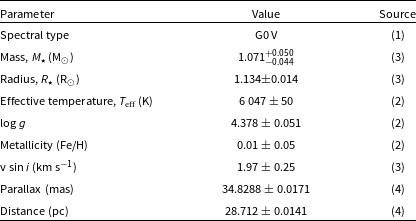
HD 38973 is a Solar-type G0 dwarf star whose salient properties are summarised in Table 1. Of particular note for our purposes here, it is a slow rotator amenable to precise RV measurements (v sin $i\lt2$
km s
$i\lt2$
km s $^{-1}$
; Soto & Jenkins Reference Soto and Jenkins2018). As such, this star has been targeted by multiple Southern Hemisphere precise RV planet-search programmes.
$^{-1}$
; Soto & Jenkins Reference Soto and Jenkins2018). As such, this star has been targeted by multiple Southern Hemisphere precise RV planet-search programmes.
Stellar parameters of HD 38973.

Table 1. Long description
The table presents the stellar parameters of HD 38973, a Solar-type G0 dwarf star. It includes seven rows and three columns, detailing the parameter, its value, and the source. The parameters listed are spectral type, mass, radius, effective temperature, log g, metallicity, v sin i, parallax, and distance. The spectral type is G0V. The mass is 1.071 plus or minus 0.050 minus 0.044 solar masses. The radius is 1.134 plus or minus 0.014 solar radii. The effective temperature is 6047 plus or minus 50 kelvin. The log g is 4.378 plus or minus 0.051. The metallicity is 0.01 plus or minus 0.05. The v sin i is 1.97 plus or minus 0.25 kilometers per second. The parallax is 34.8288 plus or minus 0.0171 milliarcseconds. The distance is 28.712 plus or minus 0.0141 parsecs. The sources for these values are cited accordingly.
Notes: (1) Gray et al. (Reference Gray2006); (2) Perdelwitz et al. (Reference Perdelwitz, Trifonov, Teklu, Sreenivas and Tal-Or2024); (3) Soto & Jenkins (Reference Soto and Jenkins2018) (4) Gaia Collaboration (Reference Gaia Collaboration2020).
HD 38973 was observed on 48 epochs from 1998 Jan 16 to 2015 Jan 30 as part of the 18-yr Anglo-Australian Planet Search (e.g. Tinney et al. Reference Tinney2001; Tinney et al. Reference Tinney2011; Wittenmyer et al. Reference Wittenmyer, Horner, Tinney, Butler, Jones, Tuomi, Salter, Carter, Koch, O’Toole, Bailey and Wright2014). Doppler RV measurements were obtained with the UCLES echelle spectrograph (Diego et al. Reference Diego, Charalambous, Fish, Walker and Crawford1990) at the 3.9-metre Anglo-Australian Telescope (AAT). A 1-arcsec slit delivers a resolving power of $R\sim 45\,000$
. The spectrograph point-spread function was calibrated using an iodine absorption cell temperature-controlled at 60.0
$R\sim 45\,000$
. The spectrograph point-spread function was calibrated using an iodine absorption cell temperature-controlled at 60.0 $ \pm $
0.1
$ \pm $
0.1 $^{\circ}$
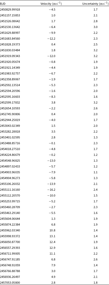
C. The iodine cell superimposes a forest of narrow absorption lines from 5 000 to 6 200 Å, allowing simultaneous calibration of instrumental drifts as well as a precise wavelength reference (Valenti et al. Reference Valenti, Butler and Marcy1995; Butler et al. Reference Butler1996). The resulting RV shift is measured relative to the epoch of the iodine-free ‘template’ spectrum. AAT velocities for HD 38973 (Appendix A, Table A1) span 17 yr and have a mean internal uncertainty of
$^{\circ}$
C. The iodine cell superimposes a forest of narrow absorption lines from 5 000 to 6 200 Å, allowing simultaneous calibration of instrumental drifts as well as a precise wavelength reference (Valenti et al. Reference Valenti, Butler and Marcy1995; Butler et al. Reference Butler1996). The resulting RV shift is measured relative to the epoch of the iodine-free ‘template’ spectrum. AAT velocities for HD 38973 (Appendix A, Table A1) span 17 yr and have a mean internal uncertainty of $2.0\,{{\mathrm{m}\,s^{-1}}}$
.
$2.0\,{{\mathrm{m}\,s^{-1}}}$
.
We also include 45 RVs from the HARPS spectrograph on the ESO 3.6m telescope at La Silla. The data used here were obtained from the HARPS RVBankFootnote
b
which provides RVs corrected for systematic errors, as well as stellar activity indicators derived from the spectra (Trifonov et al. Reference Trifonov2020; Perdelwitz et al. Reference Perdelwitz, Trifonov, Teklu, Sreenivas and Tal-Or2024). The HARPS data span 9 yr, from 2003 Oct 29 to 2012 Dec 31, and have a mean internal uncertainty of $0.9\,{{\mathrm{m\,s}^{-1}}}$
.
$0.9\,{{\mathrm{m\,s}^{-1}}}$
.
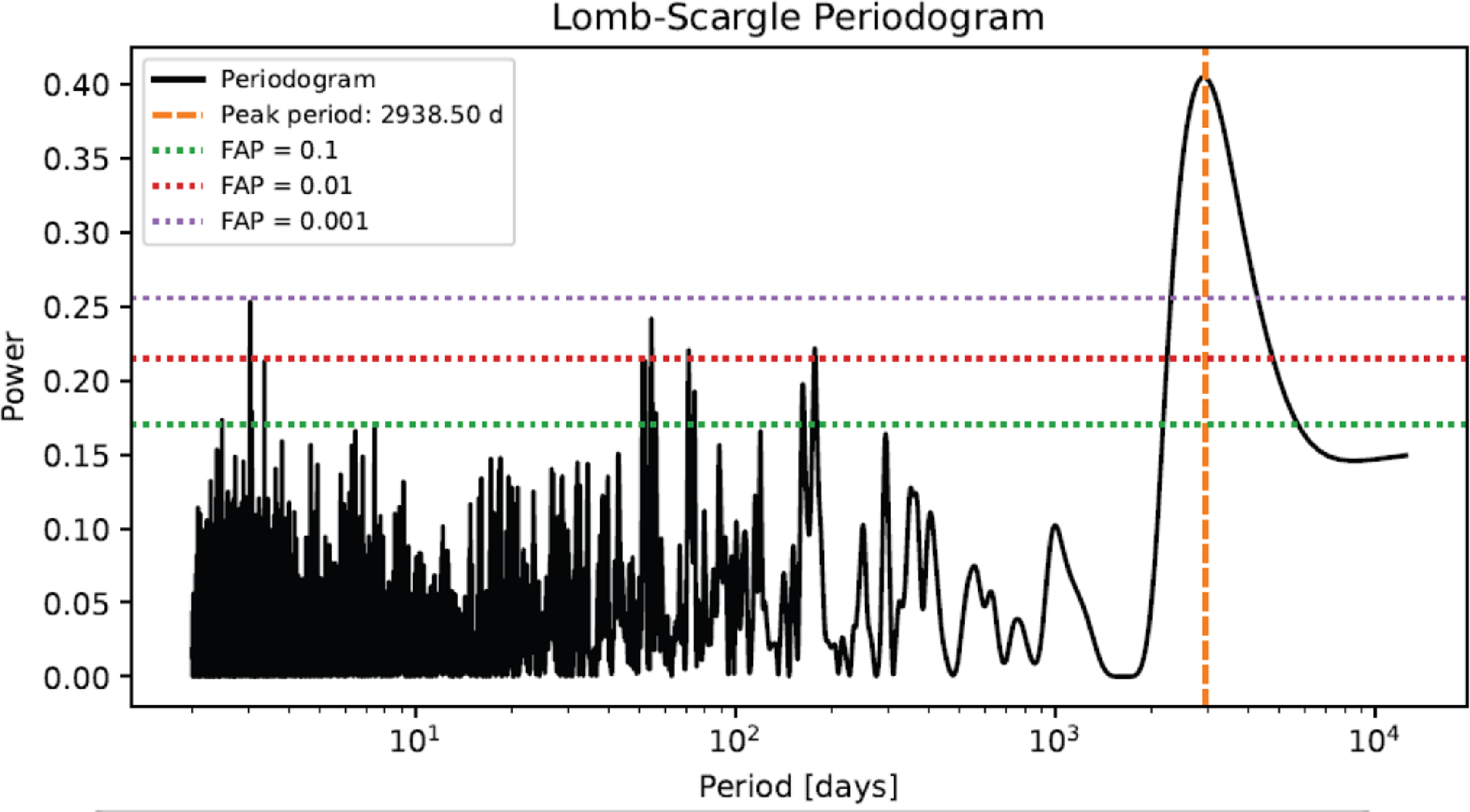
A Generalised Lomb-Scargle (GLS) periodogram of these two data sets revealed a highly significant peak near 3 000 days with a false-alarm probability $FAP=6.077\times10^{-8}$
(Figure 1). Motivated by this signal, we first carried out a preliminary orbit fit analysis using our own code, implementing a Markov Chain Monte Carlo (MCMC) approach to sample the posterior distribution of the orbital parameters. The RVs are modeled using a single-planet Keplerian of the form:
$FAP=6.077\times10^{-8}$
(Figure 1). Motivated by this signal, we first carried out a preliminary orbit fit analysis using our own code, implementing a Markov Chain Monte Carlo (MCMC) approach to sample the posterior distribution of the orbital parameters. The RVs are modeled using a single-planet Keplerian of the form:
 \begin{equation}v(t) = K \left[\cos\left(\nu(t) + \omega\right) + e \cos \omega \right] + \gamma_{\mathrm{inst}},\end{equation}
where P is the orbital period, $T_0$
the time of periastron passage, e the eccentricity,
$T_0$
the time of periastron passage, e the eccentricity, $\omega$
the argument of periastron, and K the RV semi-amplitude. Independent velocity offsets and jitter terms are included for each instrument. The AAT data feature a small (
$\omega$
the argument of periastron, and K the RV semi-amplitude. Independent velocity offsets and jitter terms are included for each instrument. The AAT data feature a small ( $\sim10\,{{\mathrm{m\,s}^{-1}}}$
) upward velocity offset that occurs near JD 2455500, which has been noted in previous analysis of other stars from that survey (Li et al. Reference Li2024). The origin of the shift remains unsolved, but as it affects more than half of the 200 Anglo-Australian Planet Search targets, with the same direction and similar magnitude, the cause is almost certainly not astrophysical. We therefore treat the AAT data as two separate sets (‘pre’ and ‘post’) with an independent offset for each.
$\sim10\,{{\mathrm{m\,s}^{-1}}}$
) upward velocity offset that occurs near JD 2455500, which has been noted in previous analysis of other stars from that survey (Li et al. Reference Li2024). The origin of the shift remains unsolved, but as it affects more than half of the 200 Anglo-Australian Planet Search targets, with the same direction and similar magnitude, the cause is almost certainly not astrophysical. We therefore treat the AAT data as two separate sets (‘pre’ and ‘post’) with an independent offset for each.
GLS periodogram analysis of the AAT and HARPS radial velocities for HD 38973. A highly significant peak is evident at $P\sim 2\,938$
days, motivating the detailed orbital and astrometric investigation presented here.
$P\sim 2\,938$
days, motivating the detailed orbital and astrometric investigation presented here.

Figure 1. Long description
A line graph titled Lomb-Scargle Periodogram displays the power of periods in days for HD 38973. The x-axis represents the period in days, ranging from 10 to 10,000 days. The y-axis represents the power, ranging from 0 to 0.4. The graph shows a significant peak at approximately 2938.50 days, indicated by an orange dashed line. The graph also includes three horizontal dashed lines representing different false alarm probability (FAP) levels: green for FAP equals 0.1, red for FAP equals 0.01, and purple for FAP equals 0.001. The periodogram line fluctuates with varying power values, showing a notable peak around the 2938.50-day mark.
The results of that initial orbital fit were then used as starting values for a more detailed analysis using RadVel (Fulton et al. Reference Fulton, Petigura, Blunt and Sinukoff2018). The uncertainties derived from the initial fit MCMC posteriors were used to apply gentle Gaussian priors on P, $T_0$
, and K, with widths equal to 5 times the
$T_0$
, and K, with widths equal to 5 times the $1\sigma$
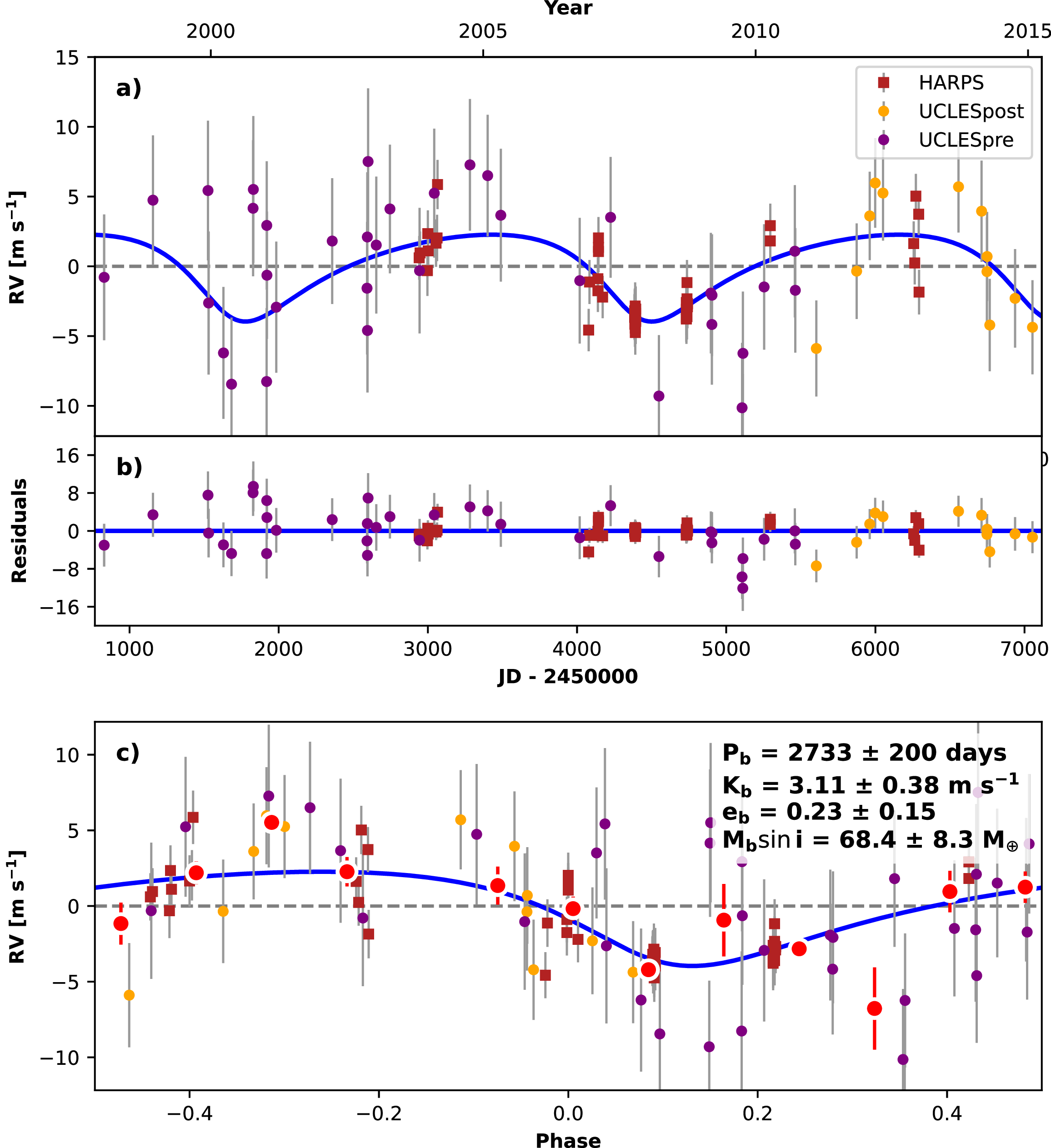
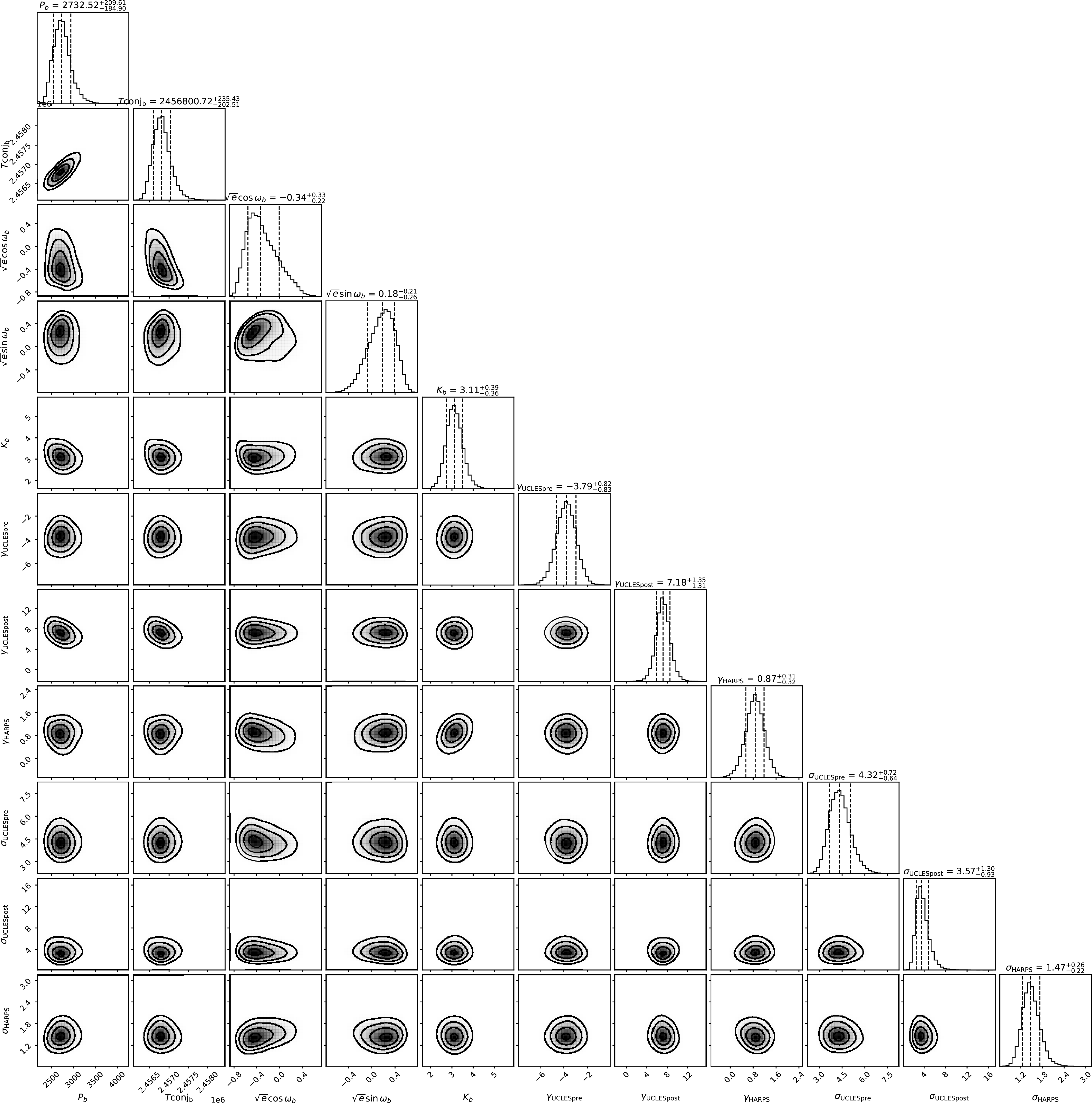
uncertainties derived previously. We show the results in Table 2 and complete corner plots are shown in the Appendix B. The adopted RadVel model fit and residuals are shown in Figure 2.
$1\sigma$
uncertainties derived previously. We show the results in Table 2 and complete corner plots are shown in the Appendix B. The adopted RadVel model fit and residuals are shown in Figure 2.
Orbital parameters of the companion inferred from the combined HARPS and AAT radial velocity data using the adopted RadVel fit. Quoted uncertainties correspond to the 16th and 84th percentiles of the posterior distributions.

Table 2. Long description
The table presents orbital parameters of a companion inferred from combined HARPS and AAT radial velocity data using the RadVel fit. It includes parameters such as orbital period, time of periastron passage, eccentricity, argument of periastron, RV semi-amplitude, systemic velocity, minimum mass, and semimajor axis. The table has eight rows and two columns. Row 1: Orbital period, P, two thousand seven hundred thirty-three days plus two hundred ten days minus three hundred seventy days. Row 2: Time of periastron passage, T zero, two million four hundred seventy-seven thousand seventy-five Julian days plus three hundred seventy days minus two hundred days. Row 3: Eccentricity, e, zero point two three plus or minus zero point zero one five. Row 4: Argument of periastron, omega, one hundred fifty-two degrees plus or minus forty-six degrees. Row 5: RV semi-amplitude, K, three point one one meters per second plus or minus zero point zero three nine meters per second minus zero point zero three seven meters per second. Row 6: Systemic velocity AAT-pre, gamma AAT-pre, negative three point seven nine meters per second plus or minus zero point zero two two meters per second minus zero point zero four meters per second. Row 7: Systemic velocity AAT-post, gamma AAT-post, seven point two two meters per second plus or minus zero point one three meters per second. Row 8: Systemic velocity HARPS, gamma HARPS, zero point eight seven meters per second plus or minus zero point zero three one meters per second minus zero point zero three two meters per second. Row 9: Minimum mass, M p sin i, zero point two two solar masses plus or minus zero point zero zero three solar masses. Row 10: Semimajor axis, a, three point nine one astronomical units plus or minus zero point zero one one astronomical units minus zero point zero one nine astronomical units.
Radial-velocity analysis of HD 38973. (a) Best-fit 1-planet Keplerian orbital model for HD 38973. The maximum likelihood model is plotted, while the orbital parameters listed in Table 2 are the median values of the posterior distributions. The thin blue line is the best fit 1-planet model. We add in quadrature the RV jitter term(s) listed in Table 2 with the measurement uncertainties for all RVs. (b) Residuals to the best fit 1-planet model. (c) RVs phase-folded to the ephemeris of planet b. The small point colours and symbols are the same as in panel a. Red circles are the same velocities binned in 0.08 units of orbital phase. The phase-folded model for planet b is shown as the blue line.

Figure 2. Long description
The image contains three graphs related to the radial-velocity analysis of HD 38973. The first graph (a) shows the best-fit 1-planet Keplerian orbital model for HD 38973. The x-axis represents the Julian Date minus 2450000, and the y-axis represents the radial velocity in meters per second. The data points are color-coded and symbolized to represent different datasets: HARPS, UCLESpost, and UCLESpre. The thin blue line represents the best-fit 1-planet model. The second graph (b) displays the residuals to the best-fit 1-planet model, with the same x-axis and y-axis as the first graph. The third graph (c) shows the radial velocities phase-folded to the ephemeris of planet b. The x-axis represents the phase, and the y-axis represents the radial velocity in meters per second. The small points are color-coded and symbolized similarly to the first graph, with additional red circles representing binned velocities. The blue line shows the phase-folded model for planet b. The graphs illustrate the orbital parameters and the fit of the model to the observed data.
Considering the stellar mass of $M_\star = 1.071^{+0.050}_{-0.044}\,{\rm M}_\odot$
(Soto & Jenkins Reference Soto and Jenkins2018), the inferred minimum mass of the companion is
$M_\star = 1.071^{+0.050}_{-0.044}\,{\rm M}_\odot$
(Soto & Jenkins Reference Soto and Jenkins2018), the inferred minimum mass of the companion is $M_p \sin i \simeq 0.22\,M_{\mathrm{ Jup}}$
, placing it well within the planetary mass regime.
$M_p \sin i \simeq 0.22\,M_{\mathrm{ Jup}}$
, placing it well within the planetary mass regime.
The value of $M \textrm{sin} i$
of 0.22
$M \textrm{sin} i$
of 0.22 $\pm$
0.03 is agnostic of the orbital inclination of the planet. Based on the RVs, it is impossible to rule out any particular inclination for the orbit – meaning that it could effectively be anywhere from edge-on to face-on. To obtain an estimate and uncertainty for the true mass of the planet, we draw inclinations for the system from a uniform distribution between zero and 90
$\pm$
0.03 is agnostic of the orbital inclination of the planet. Based on the RVs, it is impossible to rule out any particular inclination for the orbit – meaning that it could effectively be anywhere from edge-on to face-on. To obtain an estimate and uncertainty for the true mass of the planet, we draw inclinations for the system from a uniform distribution between zero and 90 $^\circ$
, and for each drawn inclination, rescale this minimum mass. The result of this exercise is detailed further in Section 4 where we incorporate astrometric information to place a constraint on the orbital inclination and hence true mass of HD 38973b. The result of this analysis for the RV data alone is a distribution of true masses, with a peak at 0.242
$^\circ$
, and for each drawn inclination, rescale this minimum mass. The result of this exercise is detailed further in Section 4 where we incorporate astrometric information to place a constraint on the orbital inclination and hence true mass of HD 38973b. The result of this analysis for the RV data alone is a distribution of true masses, with a peak at 0.242 $^{+0.140}_{-0.043}$ $M_{\rm Jup}$
.
$M_{\rm Jup}$
.
2.1 Analysis of stellar activity indicators
The period and amplitude of the RV signal we have identified here is worryingly close to the typical influences of long-term stellar magnetic cycles; a notable example being the $\sim$
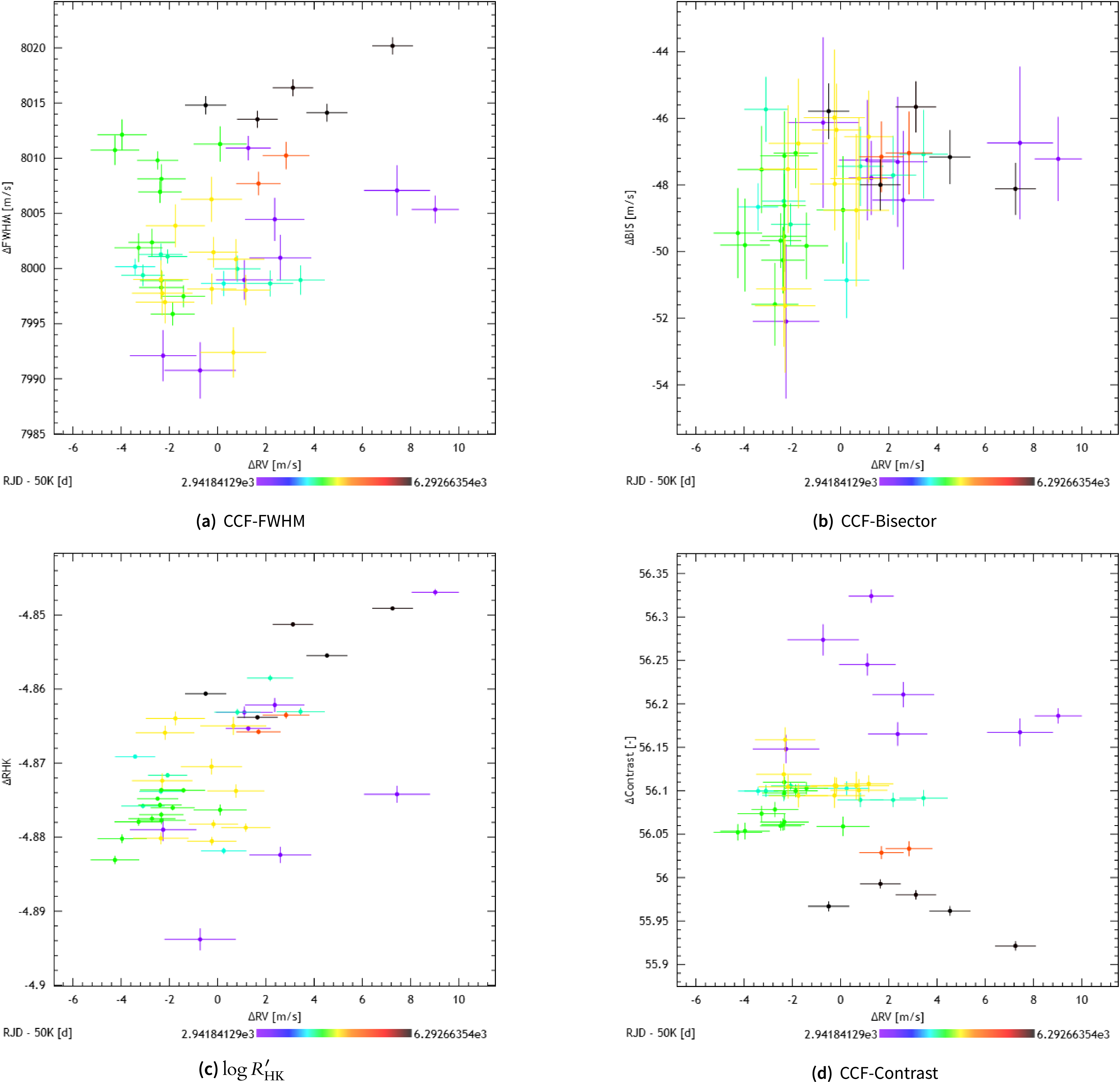
11-yr Solar cycle (e.g. Lindegren & Dravins Reference Lindegren and Dravins2003; Meunier et al. Reference Meunier, Desort and Lagrange2010). We therefore investigate several common activity indicators, which are included for the HARPS spectra. Figure 3 shows the correlations between the RV measurements and the main stellar activity indicators (FWHM, BIS,
$\sim$
11-yr Solar cycle (e.g. Lindegren & Dravins Reference Lindegren and Dravins2003; Meunier et al. Reference Meunier, Desort and Lagrange2010). We therefore investigate several common activity indicators, which are included for the HARPS spectra. Figure 3 shows the correlations between the RV measurements and the main stellar activity indicators (FWHM, BIS, $\log R'_{\mathrm{HK}}$
, and Contrast). Long-term magnetic cycles are known to induce RV signals that may mimic the presence of a planetary companion (Santos et al. Reference Santos, Gomes da Silva, Lovis and Melo2010). An analysis of HARPS Ca II H&K chromospheric activity measurements revealed no evidence of a magnetic activity cycle in HD 38973 (Lovis et al. Reference Lovis2011). Consistently, we find no significant correlations between the radial velocities and any of the activity indicators, suggesting that the observed signal is unlikely to be driven by stellar magnetic variability.
$\log R'_{\mathrm{HK}}$
, and Contrast). Long-term magnetic cycles are known to induce RV signals that may mimic the presence of a planetary companion (Santos et al. Reference Santos, Gomes da Silva, Lovis and Melo2010). An analysis of HARPS Ca II H&K chromospheric activity measurements revealed no evidence of a magnetic activity cycle in HD 38973 (Lovis et al. Reference Lovis2011). Consistently, we find no significant correlations between the radial velocities and any of the activity indicators, suggesting that the observed signal is unlikely to be driven by stellar magnetic variability.
Correlations between the radial-velocity measurements and four main stellar activity indicators: (a) FWHM, (b) CCF bisector, (c) $\log R'_{\mathrm{HK}}$
, and (d) CCF-Contrast. The colours of the points relate to the dates of observation. No significant correlations are observed in any of the panels.
$\log R'_{\mathrm{HK}}$
, and (d) CCF-Contrast. The colours of the points relate to the dates of observation. No significant correlations are observed in any of the panels.

Figure 3. Long description
The image contains four scatter plots, each depicting correlations between radial-velocity measurements and different stellar activity indicators. The x-axis in all plots represents the radial velocity (RV) in meters per second, while the y-axis represents different activity indicators: (a) FWHM in meters per second, (b) CCF bisector in meters per second, (c) log R’HK, and (d) CCF-Contrast. The data points are color-coded based on the dates of observation, ranging from purple to red. No significant correlations are observed in any of the panels. The plots are labeled as (a) CCF-FWHM, (b) CCF-Bisector, (c) log R’HK, and (d) CCF-Contrast. Each plot includes error bars indicating the uncertainty in the measurements. The overall layout shows the data points scattered without a clear trend, suggesting a lack of strong correlation between the radial-velocity measurements and the stellar activity indicators.
3. Astrometric analysis with Hipparcos-Gaia
While the RV analysis provides strong evidence for a long-period companion orbiting HD 38973, and tightly constrains P, e, $\omega$
, and K, this technique alone is insensitive to the orbital inclination and therefore yields only a minimum mass estimate. Astrometric observations with Hipparcos and Gaia can help us resolve the mass-inclination degeneracy and assess whether the companion’s true mass is compatible with the planetary regime.
$\omega$
, and K, this technique alone is insensitive to the orbital inclination and therefore yields only a minimum mass estimate. Astrometric observations with Hipparcos and Gaia can help us resolve the mass-inclination degeneracy and assess whether the companion’s true mass is compatible with the planetary regime.
3.1 Astrometric observables
As a preliminary step, we estimated the expected astrometric signal induced by the companion using the orbital parameters derived from the RV analysis. For a calculated planetary semi-major axis of $a_p = 3.866\,\mathrm{AU}$
, and mass equal to the minimum mass given in Table 2, the corresponding stellar reflex motion has an astrometric semi-major axis of
$a_p = 3.866\,\mathrm{AU}$
, and mass equal to the minimum mass given in Table 2, the corresponding stellar reflex motion has an astrometric semi-major axis of $\alpha \simeq 0.027\,\mathrm{mas}$
. This value is below the typical single-epoch astrometric precision of both Hipparcos and Gaia, and therefore a direct estimate of orbital parameters is not expected. This is also confirmed by the source’s low re-normalised unit weight error (RUWE) value of
$\alpha \simeq 0.027\,\mathrm{mas}$
. This value is below the typical single-epoch astrometric precision of both Hipparcos and Gaia, and therefore a direct estimate of orbital parameters is not expected. This is also confirmed by the source’s low re-normalised unit weight error (RUWE) value of $\sim$
1.09, below the accepted threshold of companion detectability (Penoyre et al. Reference Penoyre, Belokurov and Evans2022; Castro-Ginard et al. Reference Castro-Ginard2024). For this reason, we instead estimate an upper limit of the companion’s mass, in an attempt to confirm its planetary nature. Due to the companion’s long period of
$\sim$
1.09, below the accepted threshold of companion detectability (Penoyre et al. Reference Penoyre, Belokurov and Evans2022; Castro-Ginard et al. Reference Castro-Ginard2024). For this reason, we instead estimate an upper limit of the companion’s mass, in an attempt to confirm its planetary nature. Due to the companion’s long period of $\sim$
8 yr, we focus on the proper motion anomaly (difference between the short-term Gaia proper motion and the long-term proper motion inferred from the Hipparcos–Gaia baseline) that are sensitive to long-term accelerations (Brandt Reference Brandt2018; Brandt Reference Brandt2021). The observed proper motion anomaly is calculated by the long-term baseline proper motion (given by pmra_hg and pmdec_hg) and Gaia’s proper motion (given by pmra_gaia and pmdec_gaia) with cross-calibration and nonlinear corrections applied. For HD 38973, this is equal to
$\sim$
8 yr, we focus on the proper motion anomaly (difference between the short-term Gaia proper motion and the long-term proper motion inferred from the Hipparcos–Gaia baseline) that are sensitive to long-term accelerations (Brandt Reference Brandt2018; Brandt Reference Brandt2021). The observed proper motion anomaly is calculated by the long-term baseline proper motion (given by pmra_hg and pmdec_hg) and Gaia’s proper motion (given by pmra_gaia and pmdec_gaia) with cross-calibration and nonlinear corrections applied. For HD 38973, this is equal to
 \begin{equation}\Delta \mu_{\alpha^\ast,\mathrm{obs}} = -0.0026\pm0.0344\,\mathrm{mas/yr},\end{equation}
 \begin{equation}\Delta \mu_{\delta,\mathrm{obs}} = 0.0135\pm0.0383\,\mathrm{mas/yr}.\end{equation}
3.2 Astrometric model
For a given set of orbital parameters, the expected $\boldsymbol{\mu}$
is computed using a forward model of the stellar reflex motion induced by the companion. We first simulate photocentre offsets in the scanning direction, and fit proper motion with a method analogous to Gaia’s Astrometric Global Iterative Solution (AGIS) (Lindegren et al. Reference Lindegren2012). The observation times and scanning angles are obtained from the Gaia Observation Forecast Tool (GOST). The joint proper motion between the two catalogues is given by
$\boldsymbol{\mu}$
is computed using a forward model of the stellar reflex motion induced by the companion. We first simulate photocentre offsets in the scanning direction, and fit proper motion with a method analogous to Gaia’s Astrometric Global Iterative Solution (AGIS) (Lindegren et al. Reference Lindegren2012). The observation times and scanning angles are obtained from the Gaia Observation Forecast Tool (GOST). The joint proper motion between the two catalogues is given by
 \begin{equation} \Delta\boldsymbol{\mu}_{\rm HG} = \frac{\boldsymbol{x}(t_{G})-\boldsymbol{x}(t_{H})}{t_{G}-t_{H}} \end{equation}
where ${x}(t_{G})$
and
${x}(t_{G})$
and $\boldsymbol{x}(t_{H})$
are the offsets of the photocentre from the barycentre at the Gaia and Hipparcos reference epochs (2016.0 and 1991.25 respectively). The proper motion anomaly is then modelled by
$\boldsymbol{x}(t_{H})$
are the offsets of the photocentre from the barycentre at the Gaia and Hipparcos reference epochs (2016.0 and 1991.25 respectively). The proper motion anomaly is then modelled by
 \begin{equation}\Delta\boldsymbol{\mu}_{\mathrm{model}} = \Delta\boldsymbol{\mu}_{G}-\Delta\boldsymbol{\mu}_{\rm HG}\end{equation}
From this model, the expected proper-motion anomaly is compared directly with $\Delta\boldsymbol{\mu}_{\mathrm{obs}}$
through the HGCA covariance matrix.
$\Delta\boldsymbol{\mu}_{\mathrm{obs}}$
through the HGCA covariance matrix.
The astrometric likelihood is given by
 \begin{equation}\ln \mathcal{L}_{\mathrm{ast}} =-\frac{1}{2}\left(\Delta\boldsymbol{\mu}_{\mathrm{obs}} -\Delta\boldsymbol{\mu}_{\mathrm{model}}\right)^{\!\top}\mathbf{C}_{\Delta\mu}^{-1}\left(\Delta\boldsymbol{\mu}_{\mathrm{obs}} -\Delta\boldsymbol{\mu}_{\mathrm{model}}\right),\end{equation}
where $\mathbf{C}_{\Delta\mu}$
is the HGCA covariance matrix.
$\mathbf{C}_{\Delta\mu}$
is the HGCA covariance matrix.
3.3 Astrometric constraints from HGCA
Using the HGCA proper-motion anomaly, we evaluated the astrometric constraints on the companion mass implied by the RV solution. For a fixed orbital period, eccentricity, argument and time of periapsis inferred from RVs, we computed the expected proper-motion anomaly as a function of companion mass and orbital inclination. For each mass and inclination, the likelihood was marginalised over the longitude of the ascending node by calculating
 \begin{equation} \ln\mathcal{L}_{\mathrm{total}} = \ln\int\limits\mathcal{L}(\Omega)d\Omega.\end{equation}
Figure 4 shows the HGCA log-likelihood as a function of companion mass for threeFootnote
c
representative values of the orbital inclination. For each inclination, the likelihood curve decreases monotonically with increasing mass, reflecting the fact that more massive companions would induce larger proper-motion anomalies that are increasingly inconsistent with the HGCA measurements. The horizontal dashed line marks the threshold $\Delta \ln \mathcal{L} = -1.92$
, corresponding to a one-sided 95% confidence level for a single parameter. The intersection between each likelihood curve and this threshold defines the corresponding 95% upper limit on the companion mass for that specific inclination. These intersections therefore provide inclination-dependent upper limits on
$\Delta \ln \mathcal{L} = -1.92$
, corresponding to a one-sided 95% confidence level for a single parameter. The intersection between each likelihood curve and this threshold defines the corresponding 95% upper limit on the companion mass for that specific inclination. These intersections therefore provide inclination-dependent upper limits on $M_p$
, illustrating how the astrometric constraints strengthen as the orbit approaches a face-on configuration.
$M_p$
, illustrating how the astrometric constraints strengthen as the orbit approaches a face-on configuration.
Normalised HGCA log-likelihood as a function of companion mass for HD 38973, computed for several fixed values of the orbital inclination. For each mass and inclination, the likelihood is marginalised over the longitude of the ascending node. The horizontal dashed line indicates $\Delta\ln\mathcal{L}_{\mathrm{HGCA}}=-1.92$
, approximately corresponding to a 95% confidence upper limit on the companion mass.
$\Delta\ln\mathcal{L}_{\mathrm{HGCA}}=-1.92$
, approximately corresponding to a 95% confidence upper limit on the companion mass.

Figure 4. Long description
The line graph displays the normalized HGCA log-likelihood as a function of companion mass for HD 38973. It includes multiple lines representing different fixed values of orbital inclination. Each mass and inclination combination is marginalized over the longitude of the ascending node. A horizontal dashed line indicates a 95% confidence upper limit on the companion mass.
These results are expected to improve with the upcoming release of DR4, in late 2026, which will add a new baseline to the HGCA, even though the stellar reflex motion will still be too small for direct detection of this companion. For this study, we simulate a ‘minimum astrometric offset’ planet an edge-on orbit with mass equal to the minimum value obtained by RV. Eccentricity and argument/time of periastron were also taken from RV results. The longitude of the ascending node set to 0 $^{\circ}$
. From this, the expected proper motion anomaly was calculated by the same method as for DR3: obtaining the observation epochs from GOST, calculating the effect of the companion over DR4’s time window, and subtracting the Hipparcos-Gaia combined proper motion (Equation 4). For DR4, we use an epoch time (
$^{\circ}$
. From this, the expected proper motion anomaly was calculated by the same method as for DR3: obtaining the observation epochs from GOST, calculating the effect of the companion over DR4’s time window, and subtracting the Hipparcos-Gaia combined proper motion (Equation 4). For DR4, we use an epoch time ( $t_{G}$
) of 2017.5. This process was repeated for DR3, and the likelihood functions were combined to obtain a tighter constraint on mass. We assume the same astrometric uncertainties HGCA covariance matrix for DR3 and DR4. In reality, DR4 will most likely contain smaller uncertainties, so this can be considered a ‘worst case scenario.’
$t_{G}$
) of 2017.5. This process was repeated for DR3, and the likelihood functions were combined to obtain a tighter constraint on mass. We assume the same astrometric uncertainties HGCA covariance matrix for DR3 and DR4. In reality, DR4 will most likely contain smaller uncertainties, so this can be considered a ‘worst case scenario.’
This simulation was repeated for the DR3 baseline and the likelihoods were combined to obtain the best possible mass limit. The resultant upper mass limits from just using DR3 and Hipparcos (Figure 4) and adding in DR4 are shown in Table 3. These results strongly suggest that the astrometric signal is consistent with a planet and not a brown dwarf or low mass stellar companion.
Astrometric upper mass limits as a function of inclination using proper motion anomaly with DR3 and DR3+DR4.

Table 3. Long description
A table with three columns and four rows presents astrometric upper mass limits as a function of inclination using proper motion anomaly with DR3 and DR3+DR4 data. The columns are labeled ’Inclination’, ’DR3+HIP’, and ’DR3+DR4+HIP’. The rows list inclinations of 0.2, 0.5, and 0.8, with corresponding mass limits in solar masses. For inclination 0.2, the mass limits are 4.04 and 3.52. For inclination 0.5, the mass limits are 2.33 and 3.45. For inclination 0.8, the mass limits are 1.52 and 2.98. The table suggests that the astrometric signal is consistent with a planet rather than a brown dwarf or low-mass stellar companion.
3.4 DR2-DR3 proper motion anomaly
We investigated the possibility of also applying Gaia’s ‘internal’ proper motion anomaly between DR2 and DR3, as this would be an ideal time baseline for this companion’s period. However, after applying frame rotation calibration from (Feng et al. Reference Feng, Rui, Xuan and Jones2024) we found the magnitude of this anomaly to be $\sim$
0.2 mas/yr. A 0.22 M
$\sim$
0.2 mas/yr. A 0.22 M $_{\mathrm{J}}$
planet on an edge-on orbit would produce a proper motion anomaly magnitude of
$_{\mathrm{J}}$
planet on an edge-on orbit would produce a proper motion anomaly magnitude of $\sim$
0.006 mas/yr. In order to produce the observed magnitude, the system would need to be almost face-on (
$\sim$
0.006 mas/yr. In order to produce the observed magnitude, the system would need to be almost face-on ( $i \lt 4^{\circ}$
) which would cause an average RUWE of
$i \lt 4^{\circ}$
) which would cause an average RUWE of $\sim$
1.3, which is above the companion detection threshold for DR3 of 1.25 (Penoyre et al. Reference Penoyre, Belokurov and Evans2022; Castro-Ginard et al. Reference Castro-Ginard2024), and thus significantly higher than the catalogue value of 1.09.
$\sim$
1.3, which is above the companion detection threshold for DR3 of 1.25 (Penoyre et al. Reference Penoyre, Belokurov and Evans2022; Castro-Ginard et al. Reference Castro-Ginard2024), and thus significantly higher than the catalogue value of 1.09.
A survey of 160 sources of comparable magnitude ( $m_{G}\in[5.5,7]$
), colour (
$m_{G}\in[5.5,7]$
), colour ( $Bp-Rp\in[0.6,0.9]$
), and RUWE (
$Bp-Rp\in[0.6,0.9]$
), and RUWE ( $\lt 1.25$
) found that the proper motion anomaly is typical for this stellar sample. We, therefore, conclude that the DR2-DR3 proper motion anomaly for this source is more consistent with systematic noise than a substellar companion.
$\lt 1.25$
) found that the proper motion anomaly is typical for this stellar sample. We, therefore, conclude that the DR2-DR3 proper motion anomaly for this source is more consistent with systematic noise than a substellar companion.
4. Joint inference strategy
In order to place a more definitive constraint on the planet’s mass, we perform a joint analysis, combining our RV and astrometric analyses.
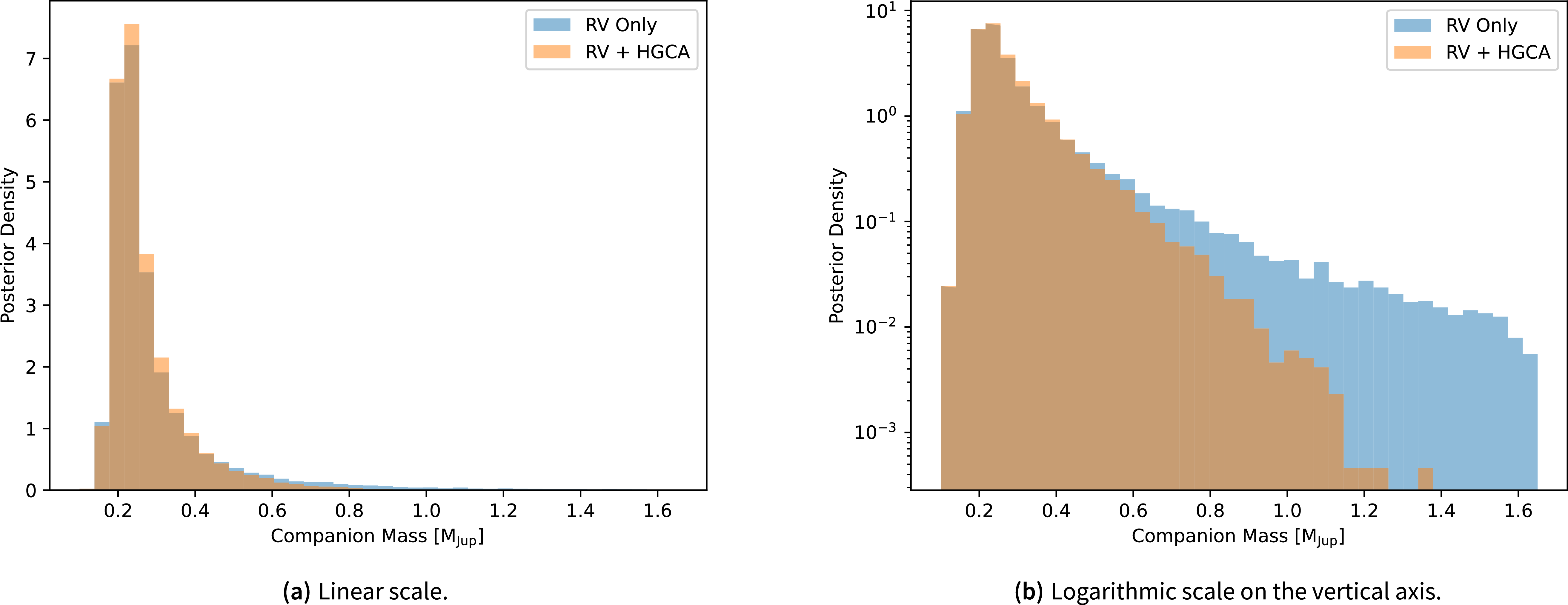
Posterior mass distributions obtained from the RV-only and joint RV and astrometric analyses. The left-hand panel shows the likelihood of different planet masses on a linear scale, with the results from the RV measurements alone illustrated in blue, and those from our joint analysis shown in orange. The right panel presents the same data but with the likelihood given on a logarithmic scale. This latter panel shows the significant impact that including the astrometric non-detection has on the tail of possible true masses that result from the sin i ambiguity inherent to RV observations.

Figure 5. Long description
A histogram showing posterior density of companion mass in Jupiter masses for RV only and RV plus HGCA analyses on linear and logarithmic scales. The left panel shows the likelihood of different planet masses on a linear scale, with the results from the RV measurements alone illustrated in blue, and those from the joint analysis shown in orange. The right panel presents the same data but with the likelihood given on a logarithmic scale. This latter panel shows the significant impact that including the astrometric non-detection has on the tail of possible true masses that result from the sin i ambiguity inherent to RV observations. The x-axis represents companion mass in Jupiter masses, ranging from 0 to 1.6. The y-axis on the left panel represents posterior density on a linear scale, while the y-axis on the right panel represents posterior density on a logarithmic scale. The blue bars represent the RV only analysis, and the orange bars represent the RV plus HGCA analysis. The histogram shows that the RV plus HGCA analysis results in a higher posterior density for lower companion masses compared to the RV only analysis. The logarithmic scale highlights the significant impact of including the astrometric non-detection on the tail of possible true masses.
Starting from the posterior samples of the RV solution, which constrain the minimum companion mass $M_p \sin i$
, we generated a distribution of true companion masses by marginalizing over the unknown orbital inclination. Assuming an isotropic distribution of orbital orientations, we drew
$M_p \sin i$
, we generated a distribution of true companion masses by marginalizing over the unknown orbital inclination. Assuming an isotropic distribution of orbital orientations, we drew $\cos i$
values from an uniform distribution in the interval (0,1) and computed the corresponding
$\cos i$
values from an uniform distribution in the interval (0,1) and computed the corresponding $\sin i$
for each realisation. The true mass for each sample was then obtained as
$\sin i$
for each realisation. The true mass for each sample was then obtained as
 \begin{equation}M_p = \frac{M_p\sin i}{\sin i}.\end{equation}
This procedure produces a broad prior distribution for the true companion mass, reflecting the geometric degeneracy inherent to RV measurements. These values illustrate the strong impact of the inclination prior on the inferred companion mass and motivate the use of external constraints, such as astrometric information, to further restrict the allowed mass range.
These summary statistics provide a compact description of the range of astrometric constraints allowed by unknown orbital orientation and are used in the following section, when combining the HGCA information with the RV results.
To combine the RV and astrometric information, we adopt a Monte Carlo approach based on the posterior samples obtained from the RV-only MCMC analysis. For each RV posterior sample, corresponding to a value of $M_p\sin i$
, an orbital inclination is randomly drawn assuming an isotropic orientation prior. For this, we assume a uniform distribution of
$M_p\sin i$
, an orbital inclination is randomly drawn assuming an isotropic orientation prior. For this, we assume a uniform distribution of $\cos i\in [0,1]$
. We ignore negative values of
$\cos i\in [0,1]$
. We ignore negative values of $\cos i$
(clockwise orbits) because, due to the small astrometric signal, this reversal of on-sky motion will have a negligible effect on likelihood. This allows us to convert the minimum mass into a true companion mass via Equation (8).
$\cos i$
(clockwise orbits) because, due to the small astrometric signal, this reversal of on-sky motion will have a negligible effect on likelihood. This allows us to convert the minimum mass into a true companion mass via Equation (8).
For each realisation, the expected proper-motion anomaly is computed and compared with the HGCA measurements by evaluating the astrometric log-likelihood marginalised over the longitude of the ascending node. These likelihood values are then used to assign statistical weights to each Monte Carlo sample, effectively downweighting orbital configurations that are incompatible with the observed proper-motion anomaly.
A weighted resampling of the Monte Carlo ensemble is performed using these astrometric likelihoods, yielding a posterior distribution for the companion mass that incorporates both the RV constraints and the HGCA non-detection.
Figure 5 presents the posterior mass distributions obtained from the RV analysis alone, and from the joint RV+HGCA solution. The left panel shows the distributions on a linear scale, facilitating a direct comparison of the median values and highest-density regions. The right panel displays the same information using a logarithmic scale on the vertical axis, highlighting differences in the tails of the distributions, and emphasising the region in which the combined analysis leads to significantly greater constraints on the planetary mass. While the RV-only solution exhibits a pronounced high-mass tail driven by the inclination degeneracy, the inclusion of astrometric constraints significantly suppresses this behaviour, yielding a more tightly constrained companion mass distribution.
From the Monte Carlo realisation of the RV posterior assuming isotropic orbital orientations, we find the mass distribution peaks at $0.242_{-0.043}^{+0.138}\,M_{\mathrm{Jup}}$
, with a 95% upper limit of
$0.242_{-0.043}^{+0.138}\,M_{\mathrm{Jup}}$
, with a 95% upper limit of $0.662\,M_{\mathrm{Jup}}$
. However, if we incorporate the astrometric information from the HGCA via likelihood weighting, we attain a peak mass of
$0.662\,M_{\mathrm{Jup}}$
. However, if we incorporate the astrometric information from the HGCA via likelihood weighting, we attain a peak mass of $0.240_{-0.040}^{+0.102}\,M_{\mathrm{Jup}}$
with a 95% upper limit of
$0.240_{-0.040}^{+0.102}\,M_{\mathrm{Jup}}$
with a 95% upper limit of $0.484\,M_{\mathrm{Jup}}$
. This demonstrates how the small astrometric signal can be used to further constrain the true mass and inclination. Specifically, these results place a minimum value on sin i of 0.5 at a 95% confidence level, which constrains the inclination to be between 27
$0.484\,M_{\mathrm{Jup}}$
. This demonstrates how the small astrometric signal can be used to further constrain the true mass and inclination. Specifically, these results place a minimum value on sin i of 0.5 at a 95% confidence level, which constrains the inclination to be between 27 $^{\circ}$
and 153
$^{\circ}$
and 153 $^{\circ}$
, and strongly rules out near-face-on orbital solutions. In the following section we place these results in a broader context, discuss their implications for the nature of the proposed companion to HD 38973, and summarise the main conclusions of this work.
$^{\circ}$
, and strongly rules out near-face-on orbital solutions. In the following section we place these results in a broader context, discuss their implications for the nature of the proposed companion to HD 38973, and summarise the main conclusions of this work.
5. Discussion and conclusions
We report the detection of a long-period RV signal in HD 38973 consistent with a sub-Jovian planetary companion on a multi-year orbit ( $P \sim 2\,733$
days). Independent Keplerian fits using HARPS and AAT data yield mutually consistent orbital solutions, supporting the robustness of the RV detection. The inferred minimum mass (
$P \sim 2\,733$
days). Independent Keplerian fits using HARPS and AAT data yield mutually consistent orbital solutions, supporting the robustness of the RV detection. The inferred minimum mass ( $M_{\rm RV}\sim0.22\pm0.03~M_{\rm Jup}$
) places the companion well within the planetary regime.
$M_{\rm RV}\sim0.22\pm0.03~M_{\rm Jup}$
) places the companion well within the planetary regime.
We explored the astrometric detectability of this signal using the Hipparcos–Gaia proper-motion anomaly formalism. The expected astrometric wobble induced by the RV solution is of order $\sim$
0.027 mas, which lies below the nominal sensitivity of both Hipparcos and Gaia for a single target. Consistent with this expectation, the measured HGCA proper-motion anomaly for HD 38973 is statistically consistent with zero.
$\sim$
0.027 mas, which lies below the nominal sensitivity of both Hipparcos and Gaia for a single target. Consistent with this expectation, the measured HGCA proper-motion anomaly for HD 38973 is statistically consistent with zero.
Despite the absence of a significant astrometric detection, the HGCA data provide meaningful constraints on the companion mass. By marginalising over the unknown longitude of the ascending node and exploring a range of orbital inclinations, we derive inclination-dependent astrometric likelihoods that exclude high-mass companions incompatible with the observed proper-motion anomaly. We further combined the astrometric information with the RV-derived posterior samples through importance reweighting. This analysis yields a 95% upper limit of 0.484 M $_{\rm Jup}$
on the true companion mass that is significantly tighter than the RV-only constraint of 0.662 M
$_{\rm Jup}$
on the true companion mass that is significantly tighter than the RV-only constraint of 0.662 M $_{\rm Jup}$
), despite the limited astrometric sensitivity in this specific case. It is clear that the combined RV+HGCA analysis robustly rules out stellar or brown-dwarf companions and confirms the planetary nature of the signal.
$_{\rm Jup}$
), despite the limited astrometric sensitivity in this specific case. It is clear that the combined RV+HGCA analysis robustly rules out stellar or brown-dwarf companions and confirms the planetary nature of the signal.
These mass upper limits show a strong dependence on inclination, as expected for long-period systems. The resultant best fit planetary mass based on our joint inference strategy for HD 38973 b is $0.240_{-0.040}^{+0.102}\,M_{\mathrm{Jup}}$
. We adopt this solution as our final, true mass determination, establishing HD 38973b as a cold sub-Saturn mass planet moving on a
$0.240_{-0.040}^{+0.102}\,M_{\mathrm{Jup}}$
. We adopt this solution as our final, true mass determination, establishing HD 38973b as a cold sub-Saturn mass planet moving on a $\sim$
7.5-yr orbit.
$\sim$
7.5-yr orbit.
Even when the expected signal lies below the detection threshold, proper-motion anomalies can exclude large regions of parameter space and place physically meaningful constraints on companion mass and inclination. As Gaia astrometry continues to improve, similar analyses will become increasingly valuable for the characterisation of long-period planets detected by radial velocities.
Our constraint on the orbital inclination of HD 38973 b also slightly increases the calculated transit probability. Assuming an isotropic distribution of inclinations, the transit probability for a planet orbiting a Sun-like star at a distance of 3.91 au is $\sim$
0.15%. For HD 38973 b, our analysis rules out orbits that are perfectly face on, and therefore increases this to 0.20%. Whilst this is only a minor change in transit probability in this case, this does demonstrate the capacity of such analysis, in the future, to help identify systems with a realistic potential for transits to be observed, through the combined use of RV and astrometric observations.
$\sim$
0.15%. For HD 38973 b, our analysis rules out orbits that are perfectly face on, and therefore increases this to 0.20%. Whilst this is only a minor change in transit probability in this case, this does demonstrate the capacity of such analysis, in the future, to help identify systems with a realistic potential for transits to be observed, through the combined use of RV and astrometric observations.
Appendix A. RV data from the AAT
AAT/UCLES Radial Velocities. Data after BJD 2455500 are treated as coming from a separate instrument with an independent velocity offset.

Appendix B. Additional figures
Corner plot of posteriors from the RadVel model fit. All parameters exhibit unimodal posteriors.

Figure B1. Long description
The image displays a corner plot of posteriors from the RadVel model fit. It consists of multiple graphs arranged in a grid, with each cell containing either a contour plot or a histogram. The contour plots show the relationships between different pairs of parameters, with darker regions indicating higher probability densities. The histograms along the diagonal represent the marginal distributions of individual parameters. All parameters exhibit unimodal posteriors, suggesting a single peak in their probability distributions. The plot provides a comprehensive visualization of the model’s parameter space, highlighting the correlations and distributions of the fitted parameters.
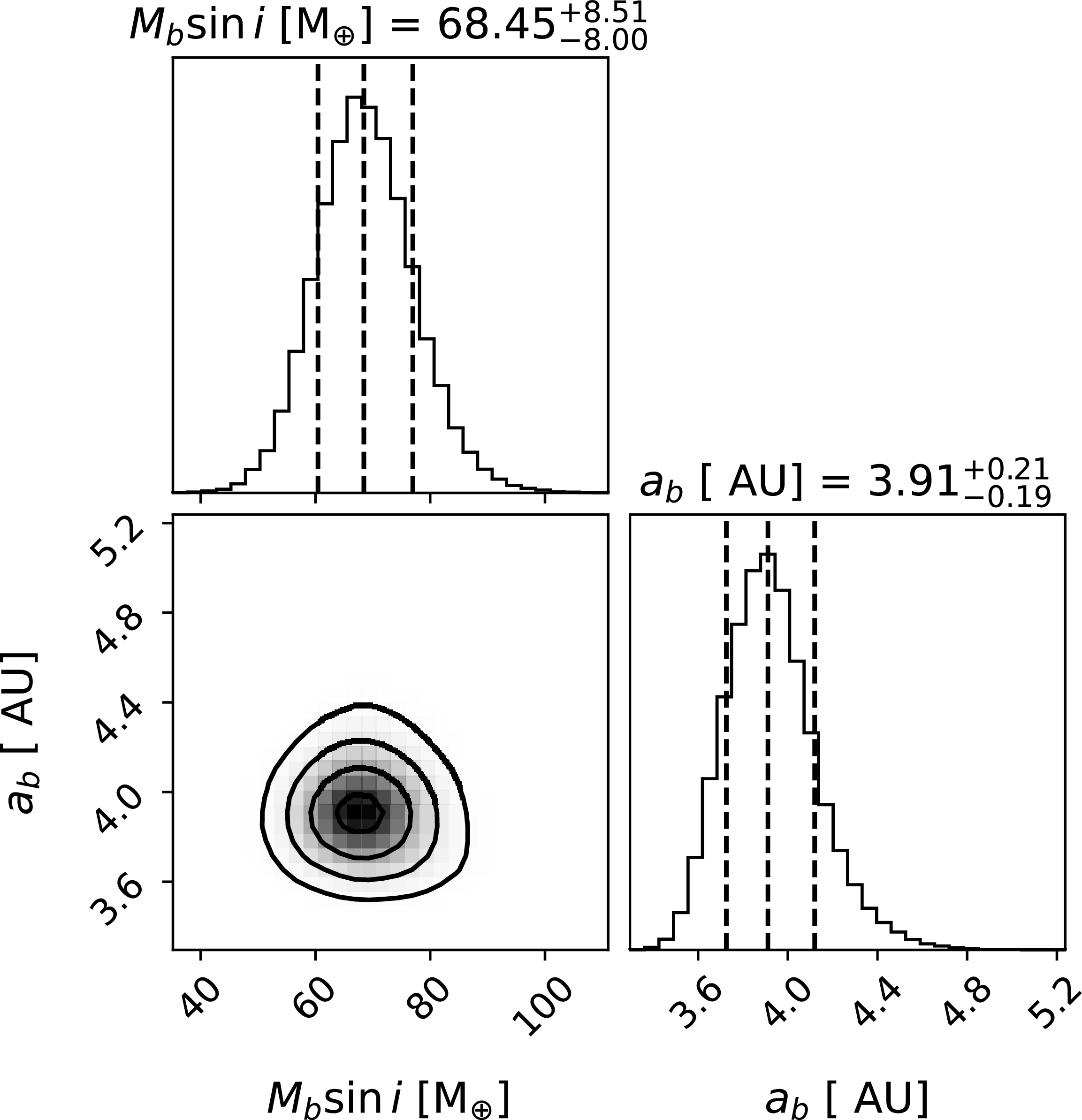
Corner plot of MCMC posteriors for the derived planetary parameters a and $M_p \sin i$
.
$M_p \sin i$
.

Figure B2. Long description
The image contains a corner plot showing MCMC posteriors for the derived planetary parameters semi-major axis (a) and mass times sine of inclination (M sin i). The plot consists of three subplots: two histograms and one contour plot. The top-left histogram shows the distribution of M sin i in Earth masses, with a mean value of 68.45 Earth masses and uncertainties of plus or minus 8.51 and 8.00 Earth masses. The bottom-right histogram displays the distribution of semi-major axis (a) in astronomical units, with a mean value of 3.91 astronomical units and uncertainties of plus or minus 0.21 and 0.19 astronomical units. The bottom-left contour plot shows the joint distribution of M sin i and a, with contours indicating different probability density levels. The histograms and contour plot together illustrate the relationships and uncertainties in the derived planetary parameters.
 P∼2938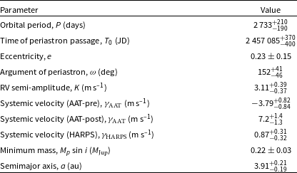
 logRHK′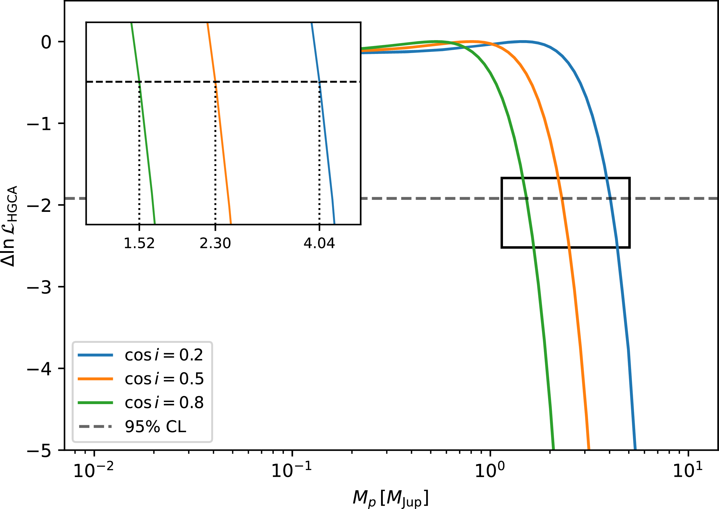
 ΔlnLHGCA=−1.92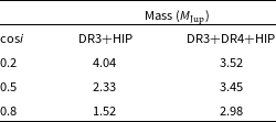
 Mpsini
 Open access

