





Impact Statement
Many structures operate under highly variable, task-dependent conditions, making reliable anomaly detection challenging in practice. Conventional methods often rely on a single reference condition, an assumption violated when systems switch between discrete operating regimes, causing early deviations to be masked. This work proposes an efficient probabilistic framework in which each operating regime is represented by a local dynamic model. A Bayesian formulation accounts explicitly for uncertainty arising from limited and noisy data and enables sequential updating as new data becomes available—particularly advantageous for early-stage deployment. New observations are assessed through statistical consistency, allowing operational changes to be distinguished from anomalies that may indicate structural change. The method is demonstrated using vibration data from a working vessel in operation.
1. Introduction
Structural Health Monitoring (SHM) systems are playing an increasingly important role in ensuring the continued reliability and operational safety of structures. Such systems leverage measured data—for example, vibrational response of the structure—collected over a range of operational conditions to assess structural integrity without interrupting normal usage. However, one of the major challenges in SHM lies in accounting for the influence of operational variability on the structural response. As operating conditions fluctuate—for example, due to load changes, environmental influences, or variations in usage—the response of the structure is likely to change even in the absence of degradation, making it difficult to distinguish between normal operational variation and true structural degradation. This challenge has received increasing attention in recent years, with several studies proposing methods to account for operational variability within SHM frameworks (Dackermann et al., Reference Dackermann, Li and Samali2013; Martinez-Luengo et al., Reference Martinez-Luengo, Kolios and Wang2016; Avendaño-Valencia and Chatzi, Reference Avendaño-Valencia and Chatzi2020; Keshmiry et al., Reference Keshmiry, Hassani, Mousavi and Dackermann2023). Despite these efforts, effectively distinguishing between changes due to structural degradation and changes due to varying operational conditions remains a fundamental challenge. Addressing this is crucial for ensuring reliable damage detection and the effectiveness of SHM systems.
The well-established procedures for addressing the influence of Environmental and Operational Variability (EOV) can be categorized into explicit and implicit methods. Explicit methods can be seen as cause-effect methods where measured Environmental and Operational Parameters (EOPs) are correlated with the dynamic characteristics of the structure through mathematical models (García Cava et al., Reference García Cava, Avendaño-Valencia, Movsessian, Roberts, Tcherniak, Cury, Ribeiro, Ubertini and Todd2022). Such models can be deterministic regression models based on the assumption that the relationship between EOPs and the dynamic characteristics is deterministic (Schlechtingen and Ferreira Santos, Reference Schlechtingen and Ferreira Santos2011; Bogoevska et al., Reference Bogoevska, Spiridonakos, Chatzi, Dumova-Jovanoska and Höffer2017). However, different sources of uncertainties—for example, unmeasured EOPs—challenge the assumption of a deterministic approach. For this, a variety of probabilistic models, like Bayesian and Gaussian process regression models, have been investigated (Avendaño-Valencia et al., Reference Avendaño-Valencia, Chatzi and Tcherniak2020; García-Macías and Ubertini, Reference García-Macías and Ubertini2022; Drangsfeldt and Avendaño-Valencia, Reference Drangsfeldt and Avendaño-Valencia2024). In the context of rotating machinery, synchronization-based techniques are typically employed to mitigate operational variability resulting from speed changes by aligning the vibrational response with shaft rotation (Randall et al., Reference Randall, Sawalhi and Coats2012; Randall et al., Reference Randall, Smith and Coats2014). Implicit methods, on the other hand, can be seen as effect-only methods. Here, the procedure is to transform the data into a space where the influence of EOV can effectively be mitigated. One of the often used methods is Principal Component Analysis (PCA), which assumes that most variance is caused by EOV and mitigates its influence by transforming the data and discarding those latent variables that capture the largest variance (Yan et al., Reference Yan, Kerschen, De Boe and Golinval2005; Cross et al., Reference Cross, Manson, Worden and Pierce2012; Deraemaeker and Worden, Reference Deraemaeker and Worden2018). However, explicit methods are challenged by the fact that the EOV arises from complex interactions among multiple EOPs, many of which are unknown or unmeasurable. Likewise, synchronization-based techniques are challenged if the shaft speed is unmeasured. The shaft speed can be estimated from the vibrational response; however, measurement noise and non-stationarity in the signal can obscure the accuracy of the estimation. Also, implicit methods carry the risk that variance caused by structural changes may be entangled with EOV, potentially leading to the loss of damage-relevant information (Drangsfeldt and Avendaño-Valencia, Reference Drangsfeldt and Avendaño-Valencia2024). Most importantly, both explicit and implicit methods face additional challenges when the operation consists of discrete operating regimes. In such cases, the structural characteristics themselves appear as multiple distinct regimes, and the variability between regimes may overshadow subtle structural changes within a regime.
When the system operates across multiple discrete regimes, a natural approach is to segment the operation accordingly and treat each regime as a local representation of the global system—an approach referred to as a multi-model approach. In the context of a functional SHM system, it is crucial to distinguish between these local representations, as each has its own characteristic structural behavior and corresponding reference condition. Damage assessment must therefore be performed by comparing estimated Damage Sensitive Features (DSFs) against the appropriate reference state within the same regime to ensure meaningful and reliable evaluation. For systems where the operating regimes are governed by measured operational parameters, thresholds on these parameters can be defined and used to distinguish between regimes (Avendaño-Valencia et al., Reference Avendaño-Valencia, Chatzi and Tcherniak2020; Nguyen Khac et al., Reference Nguyen Khac, Zenger, Storm and Hyvönen2020). However, for systems where the regimes are governed by a complex combination of a variety of conditions, distinguishing between them becomes more challenging. Several approaches have been investigated to distinguish between operating regimes, such as clustering techniques (Avendaño-Valencia and Fassois, Reference Avendaño-Valencia and Fassois2017; Zhang et al., Reference Zhang, Bingham, Martínez-García and Cox2017), simple decision tree structures (Chen et al., Reference Chen, Meng, Jia and Kuang2021; Sørensen et al., Reference Sørensen, Lutzen, Eriksen and Jensen2022), probabilistic approaches utilizing a Markov transition process (Liu et al., Reference Liu, Wang, Bornn and Farrar2019; Drangsfeldt et al., Reference Drangsfeldt, Avendaño-Valencia and Lützen2026), and multi-model approaches based on best-fit selection criteria (Vlachospyros et al., Reference Vlachospyros, Fassois and Sakellariou2024). The advantage of representing the global system through a pool of local models is that it mitigates the significant variability between operating regimes. This facilitates the application of both explicit methods—such as regression models and synchronization-based techniques—and implicit methods, each tailored to the corresponding local representation. As a result, the SHM process can be carried out more reliably within each regime.
Within the multi-model framework, DSFs are used to represent the local condition of the structure, where a pool of local representations forms the global representation. To ensure sensitivity to structural changes, it is important to select appropriate DSFs, as the optimal choice may depend on the specific application. Various DSFs have been investigated, mainly divided into physical DSFs and abstract DSFs. In the physical domain, typical DSFs include estimated modal parameters of the structure, primarily natural frequencies, and mode shapes (Hansen et al., Reference Hansen, Brincker, López-Aenlle, Overgaard and Kloborg2017; Gorgin and Wang, Reference Gorgin and Wang2020; Chandrasekhar et al., Reference Chandrasekhar, Stevanovic, Cross, Dervilis and Worden2021). Additionally, damping ratios have been shown to exhibit greater sensitivity to structural damage than natural frequencies, and mode shapes (Cao et al., Reference Cao, Sha, Gao and Ostachowicz2017). In the context of rotating machinery, physical features commonly used are typically linked to specific components, such as bearings and gears. Each one provides a unique signature in the frequency domain, which can serve as DSFs (Randall, Reference Randall2011; Randall et al., Reference Randall, Sawalhi and Coats2012). In the abstract domain, features are not directly linked to the structure’s dynamics but may encapsulate global vibration behavior in a small number of variables. These can include parameters from non-parametric representations of the vibrational response, such as Power Spectral Density (PSD) estimates Universitat Ramon (Font-Moré et al., Reference Font-Moré, Garcia Cava, Perez and Avendano-Valencia2024), as well as parameters from parametric models, where variants of Autoregressive (AR) models have been widely used (Roy et al., Reference Roy, Bhattacharya and Ray-Chaudhuri2015; Avendaño-Valencia et al., Reference Avendaño-Valencia, Chatzi and Tcherniak2020; Drangsfeldt and Avendaño-Valencia, Reference Drangsfeldt and Avendaño-Valencia2024). While the abstract features often have higher dimensionality than the physical features, they are typically the parameters of the models used to estimate the physical features. Therefore, they contain at least the same damage-related information as the physical features—potentially even more (Drangsfeldt and Avendaño-Valencia, Reference Drangsfeldt and Avendaño-Valencia2024).
To accurately represent each local condition of the structure, the representation must account for all sources of variability. Additionally, understanding how DSFs behave under structural degradation is essential for determining when the structure should be classified as damaged. However, environmental variability often evolves slowly through seasonal changes (Keshmiry et al., Reference Keshmiry, Hassani, Mousavi and Dackermann2023), which necessitates a comprehensive database to capture its full effect. Even if such a database is available, rare or extreme events are still likely to be missing. Furthermore, data reflecting structural degradation is typically unavailable, as it requires the structure to have been in service for many years. As a result, building a sufficiently comprehensive database capturing all relevant variability and degradation scenarios to ensure robust SHM is often infeasible. This limitation has motivated the development of alternative methods. One approach involves estimating short-time-scale AR or Autoregressive with Exogenous inputs (ARX) models as local representations of the structure’s dynamics, followed by Gaussian Process regression to model the dependence of operational conditions once a full operational cycle has been observed (Avendaño-Valencia et al., Reference Avendaño-Valencia, Chatzi, Koo and Brownjohn2017; Tatsis et al., Reference Tatsis, Dertimanis, Ou and Chatzi2020). Another approach is to adopt a fully Bayesian framework, which treats the parameters of the chosen model as random variables and systematically updates prior knowledge as new observations become available. In the context of SHM, this has been applied to a local Linear Parameter Varying (LPV) AR model, where each local representation is assumed to correspond to a stationary part of the full EOV (Avendaño-Valencia, Reference Avendaño-Valencia2025). Other studies have proposed Bayesian updating frameworks that, while not strictly recursive, support robust SHM under uncertainty and limited measurements (Chen et al., Reference Chen, Zhang, Zheng and Sun2020; Li et al., Reference Li, Huang and Asadollahi2021; García-Macías and Ubertini, Reference García-Macías and Ubertini2022). In parallel, Bayesian approaches have been proposed for handling incomplete SHM data, including methods for missing data imputation and uncertainty quantification (Wang et al., Reference Wang, Liu, Ma, Wang, Ni, Ren and Wang2024; Wang et al., Reference Wang, Huang, Ni, Feng, Wang, Qiu, Zhou, Li and Luo2026).
For systems operating under multiple discrete regimes, both explicit and implicit strategies for mitigating EOV may face significant challenges, as previously discussed. The multi-model framework provides a means to incorporate these techniques within each local representation of the system. However, variability can persist even at the local scale due to complex interactions among multiple EOPs, many of which are unknown, unmeasurable, or both. Moreover, in practice, critical parameters—such as RPM in rotating machinery—are not always available due to sensor limitations or confidentiality constraints, which further complicates the application of conventional approaches. For rotating machinery, frequency components associated with specific components are commonly used as DSFs. However, when the measured RPM is unavailable, the use of these features requires greater caution, as their interpretation depends on accurate alignment with the machine’s operating speed. Moreover, as previously discussed, abstract features may encapsulate even more damage-related information than physical features, especially in cases where direct physical interpretation is limited or compromised. This challenge also extends to the use of modal parameters as DSFs. While these parameters are directly linked to the structure’s dynamic behavior, their accurate estimation—particularly of damping ratios—can be difficult in practice. Additionally, not all modes may be sufficiently excited by the operating environment to be observable in the measured vibrational response. Overall, various sources of uncertainty exist—including the appropriate division of local representations, the selection of suitable DSFs, and the influence of EOV—all of which support the use of a probabilistic framework to model this uncertainty. A Bayesian updating framework is particularly advantageous in the preliminary phase of an SHM system, where data may be sparse and uncertainty high.
To address the challenges identified above, this paper proposes a sequentially updating Bayesian multi-model time-series framework for Vibration-Based Structural Health Monitoring (VBSHM). The objective is to enable robust VBSHM for systems operating across multiple discrete regimes, even when key operational parameters are unmeasured or unavailable. The framework combines local time-series modeling using Vector Autoregressive (VAR) models—with each capturing system dynamics at a local scale—with a fully Bayesian formulation that enables uncertainty quantification and sequential updating of local representations that function as local references. Specifically, the parameters of the local VAR models are represented by posterior distributions, which constitute the DSFs and are sequentially updated as observations are received. When observations from an unknown structural condition are received, the likelihood of each local VAR model fitting the new observations is evaluated. The model with the highest likelihood is selected as the best-fit operating regime. At the same time, the magnitude of the likelihood—or the deviation from the regime model—serves as an indicator of anomalies, corresponding to deviations from the established reference. These deviations may arise from structural changes, maintenance actions, or damage, depending on the available data. The approach is particularly suited for early-phase SHM development, where data are sparse, and uncertainty is high, limiting the effectiveness of conventional techniques. To demonstrate its applicability, the framework is tested using the vibrational response measured from a gearbox in the propulsion unit of a Crew Transfer Vessel (CTV). In this case, the preliminary nature of the SHM system and confidentiality constraints—such as inaccessible RPM measurements and internal gearbox details—highlight the practical challenges addressed by the proposed framework. In addition, the performance of the proposed framework tested on the case study is compared against a benchmark representing a traditional SHM approach adopted from Drangsfeldt and Avendaño-Valencia (Reference Drangsfeldt and Avendaño-Valencia2024). This benchmark is based on using the parameters of VAR models as DSFs, combined with implicit mitigation of EOV through PCA.
The remainder of this paper is organized as follows: Section 2 outlines the proposed multi-model and the underlying methods. Section 3 describes the case study, where the measured vibrational response of a gearbox is used to demonstrate both the benchmark approach and the proposed framework, and their implementation. Section 4 presents the results of the implemented multi-model framework for VBSHM. These results are then discussed in Section 5, with concluding remarks provided in Section 6.
2. Methodology
The general process of the multi-model framework is illustrated in Figure 1. The framework is built upon the Bayesian VAR model introduced in Section 2.1, where the model parameters
$ \left\{\boldsymbol{\Theta}, {\boldsymbol{\Sigma}}_w\right\} $
 act as DSFs. For systems operating under time-varying conditions, the full operation is represented through a set of
$ K $
act as DSFs. For systems operating under time-varying conditions, the full operation is represented through a set of
$ K $
 operating regimes, where each regime
$ k\in \left[1,2,\dots, K\right] $
operating regimes, where each regime
$ k\in \left[1,2,\dots, K\right] $
 is characterized by regime-specific posterior hyperparameters
$ {\boldsymbol{\beta}}_k^{\left(\mathrm{post}\right)} $
is characterized by regime-specific posterior hyperparameters
$ {\boldsymbol{\beta}}_k^{\left(\mathrm{post}\right)} $
 , comprising local reference models. These local references can be defined either using prior knowledge of operating regimes (supervised setting) or inferred directly from data (unsupervised setting), as described in Section 2.3. The hyperparameters are inferred from data representative of the normal behavior of the system and may be updated sequentially as new observations become available. Together, these define a set of regime-conditioned Bayesian VAR models that capture the variability of the system under different operating conditions.
Flowchart of the multi-model approach.
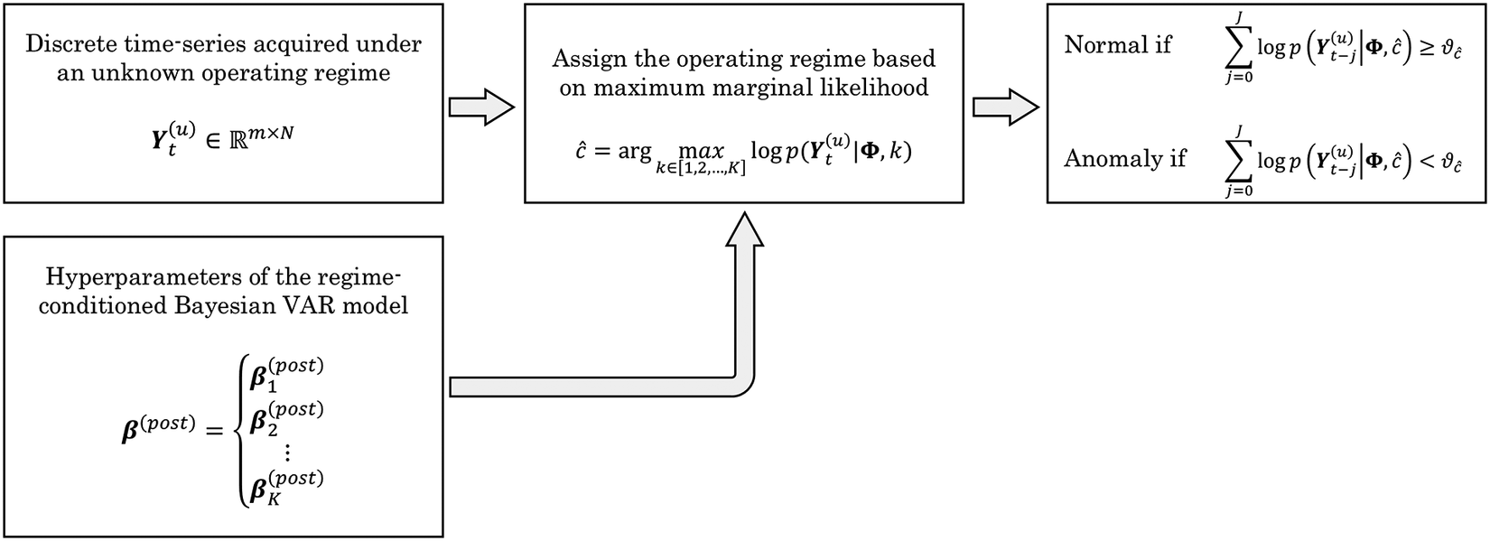
Figure 1. Long description
The flowchart consists of four main blocks connected by arrows.
* Top-left block: Input data described as Discrete time-series acquired under an unknown operating regime. The mathematical notation is Y sub t super (u) in R super m times N. An arrow points right to the central block.
* Bottom-left block: Model parameters described as Hyperparameters of the regime-conditioned Bayesian V A R model. The notation is beta super (post) equals a set containing beta sub 1 super (post), beta sub 2 super (post), through beta sub K super (post). An L-shaped arrow points from this block up into the central block.
* Central block: Processing step described as Assign the operating regime based on maximum marginal likelihood. The equation is c-hat equals arg max over k in the set 1, 2, to K of log p (Y sub t super (u) vertical bar Phi, k). An arrow points right to the final block.
* Right block: Classification output with two conditions.
1. Normal if the summation from j equals 0 to J of log p (Y sub t minus j super (u) vertical bar Phi, c-hat) is greater than or equal to theta sub c-hat.
2. Anomaly if the same summation is less than theta sub c-hat.
In operation, a new multichannel time-series segment
$ {\boldsymbol{Y}}_t^{(u)}\in {\unicode{x211D}}^{m\times N} $
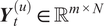 , where
$ m $
, where
$ m $
 is the number of channels and
$ N $
is the number of channels and
$ N $
 is the number of discrete samples, is acquired under an unknown operating regime, and the associated regression matrix
$ \boldsymbol{\Phi} \in {\unicode{x211D}}^{d\times \tau } $
is the number of discrete samples, is acquired under an unknown operating regime, and the associated regression matrix
$ \boldsymbol{\Phi} \in {\unicode{x211D}}^{d\times \tau } $
 is constructed, where
$ d=m\cdot {n}_a $
is constructed, where
$ d=m\cdot {n}_a $
 with
$ {n}_a $
with
$ {n}_a $
 being the model order of the VAR model and
$ \tau =N-{n}_a $
being the model order of the VAR model and
$ \tau =N-{n}_a $
 . Rather than explicitly estimating
$ \boldsymbol{\Theta} $
. Rather than explicitly estimating
$ \boldsymbol{\Theta} $
 and
$ {\boldsymbol{\Sigma}}_w $
and
$ {\boldsymbol{\Sigma}}_w $
 , the model parameters are analytically marginalized, yielding a closed-form expression for the log marginal likelihood
$ \log p\left({\boldsymbol{Y}}_t^{(u)}|\boldsymbol{\Phi}, k\right) $
, the model parameters are analytically marginalized, yielding a closed-form expression for the log marginal likelihood
$ \log p\left({\boldsymbol{Y}}_t^{(u)}|\boldsymbol{\Phi}, k\right) $
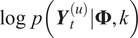 under each local reference model. Among the existing operating regimes, the one that maximizes the log marginal likelihood is selected as the most probable explanation of the observed data segment. To assess anomalies in the system, such as structural changes, the anomaly detection is not performed based on individual segments, but rather on an accumulated statistic over a sliding window of recent observations. This enables robust identification of persistent deviations from the learned reference behavior while reducing sensitivity to transient outliers, as detailed in Section 2.3.1.
The multi-model framework and formulations, together with the procedure stated above, are detailed in the following sections.
2.1. Vector Autoregressive models
A VAR model can be used as a parametrized representation of a multichannel discrete-time series
$ \boldsymbol{Y}\in {\unicode{x211D}}^{m\times N} $
 for which stationarity of
$ \boldsymbol{Y} $
for which stationarity of
$ \boldsymbol{Y} $
 is a fundamental requirement, implying that the model parameters are time-invariant over the analysis period (Farrar and Worden, Reference Farrar and Worden2012, p. 233). The VAR model is an extension of the conventional AR model, enabling the joint modeling of multiple, potentially coupled signals. Modeling each signal independently may neglect important cross-channel dependencies, whereas the VAR formulation captures both dynamics within each channel and the coupling between channels. The VAR model is formulated as:

where
$ \boldsymbol{y}\left[t\right]\in {\unicode{x211D}}^m $
 is a column vector of multichannel observations in
$ \boldsymbol{Y} $
is a column vector of multichannel observations in
$ \boldsymbol{Y} $
 at time
$ t $
at time
$ t $
 . The AR parameters at the given time lag
$ i $
. The AR parameters at the given time lag
$ i $
 are represented in the matrix
$ {\boldsymbol{A}}_i\in {\unicode{x211D}}^{m\times m} $
are represented in the matrix
$ {\boldsymbol{A}}_i\in {\unicode{x211D}}^{m\times m} $
 . The vector
$ \boldsymbol{w}\left[t\right]\in {\unicode{x211D}}^m $
. The vector
$ \boldsymbol{w}\left[t\right]\in {\unicode{x211D}}^m $
 denotes the zero-mean normally and independently distributed innovations, which represent the part of the stochastic process that cannot be predicted from the previous
$ {n}_a $
denotes the zero-mean normally and independently distributed innovations, which represent the part of the stochastic process that cannot be predicted from the previous
$ {n}_a $
 samples. These innovations are distributed with the innovation covariance matrix
$ {\boldsymbol{\Sigma}}_w\in {\unicode{x211D}}^{m\times m} $
samples. These innovations are distributed with the innovation covariance matrix
$ {\boldsymbol{\Sigma}}_w\in {\unicode{x211D}}^{m\times m} $
 (Farrar and Worden, Reference Farrar and Worden2012, Ch. 7.11). This structure can be compactly written for the complete time-series from the
$ {n}_a+1 $
(Farrar and Worden, Reference Farrar and Worden2012, Ch. 7.11). This structure can be compactly written for the complete time-series from the
$ {n}_a+1 $
 observation to the
$ {N}^{\mathrm{th}} $
observation to the
$ {N}^{\mathrm{th}} $
 observation, denoted as
$ {\boldsymbol{Y}}_{\tau } $
observation, denoted as
$ {\boldsymbol{Y}}_{\tau } $
 , as:
, as:

where the innovations in
$ \boldsymbol{W}=\left[\boldsymbol{w}\left[{n}_a+1\right]\hskip0.5em \boldsymbol{w}\left[{n}_a+2\right]\hskip0.5em \cdots \hskip0.5em \boldsymbol{w}\left[N\right]\right] $
 are independent across
$ t $
are independent across
$ t $
 . The complete set of AR parameters is stacked in the matrix
$ \boldsymbol{\Theta} \in {\unicode{x211D}}^{m\times d} $
. The complete set of AR parameters is stacked in the matrix
$ \boldsymbol{\Theta} \in {\unicode{x211D}}^{m\times d} $
 with
$ d={mn}_a $
with
$ d={mn}_a $
 , and the lagged observations are stacked in the regression matrix
$ \boldsymbol{\Phi} \in {\unicode{x211D}}^{d\times \tau } $
, and the lagged observations are stacked in the regression matrix
$ \boldsymbol{\Phi} \in {\unicode{x211D}}^{d\times \tau } $
 where
$ \tau =N-{n}_a $
where
$ \tau =N-{n}_a $
 such that:

Classically, estimation of the AR parameters
$ \boldsymbol{\Theta} $
 and innovations covariance
$ {\boldsymbol{\Sigma}}_w $
and innovations covariance
$ {\boldsymbol{\Sigma}}_w $
 is performed by means of a Least Squares approach, where the objective is to minimize the sum of squared differences between the observed values and the model predictions (Hastie et al., Reference Hastie, Tibshirani and Friedman2009, pp. 11–12):
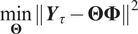
which leads to the solution:

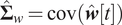
where the innovations can be estimated as:

and the innovation covariance as:
This estimation assumes that
$ \boldsymbol{\Theta} $
 and
$ {\boldsymbol{\Sigma}}_w $
and
$ {\boldsymbol{\Sigma}}_w $
 are fixed, deterministic values, implicitly requiring that the available data are sufficient to estimate them accurately and that no parameter uncertainty remains—an assumption that is rarely satisfied in real-life applications. To account for this uncertainty,
$ \boldsymbol{\Theta} $
are fixed, deterministic values, implicitly requiring that the available data are sufficient to estimate them accurately and that no parameter uncertainty remains—an assumption that is rarely satisfied in real-life applications. To account for this uncertainty,
$ \boldsymbol{\Theta} $
 and
$ {\boldsymbol{\Sigma}}_w $
and
$ {\boldsymbol{\Sigma}}_w $
 may instead be treated as random variables. However, this requires alternative estimation methods.
2.1.1. Bayesian-formulated VAR models
While the least squares solution in Equations (5)–(7) treats
$ \boldsymbol{\Theta} $
 and
$ {\boldsymbol{\Sigma}}_w $
and
$ {\boldsymbol{\Sigma}}_w $
 as fixed quantities, a Bayesian formulation recognizes that, in practice, these parameters are uncertain—particularly when they are estimated from short data segments, when operating conditions fluctuate, or when the signal-to-noise ratio is low. Under such conditions, the ordinary Least Squares estimator is prone to overfitting, producing parameter estimates that adapt too closely to noise rather than to the underlying system dynamics. By modeling
$ \boldsymbol{\Theta} $
as fixed quantities, a Bayesian formulation recognizes that, in practice, these parameters are uncertain—particularly when they are estimated from short data segments, when operating conditions fluctuate, or when the signal-to-noise ratio is low. Under such conditions, the ordinary Least Squares estimator is prone to overfitting, producing parameter estimates that adapt too closely to noise rather than to the underlying system dynamics. By modeling
$ \boldsymbol{\Theta} $
 and
$ {\boldsymbol{\Sigma}}_w $
and
$ {\boldsymbol{\Sigma}}_w $
 as random variables, the Bayesian approach explicitly accounts for this estimation uncertainty and introduces prior structure that stabilizes the inference, especially in regimes where data are limited or highly variable. In the Bayesian VAR formulation, each observation
$ \boldsymbol{y}\left[t\right] $
as random variables, the Bayesian approach explicitly accounts for this estimation uncertainty and introduces prior structure that stabilizes the inference, especially in regimes where data are limited or highly variable. In the Bayesian VAR formulation, each observation
$ \boldsymbol{y}\left[t\right] $
 is conditioned on the model parameters
$ \boldsymbol{\Theta} $
is conditioned on the model parameters
$ \boldsymbol{\Theta} $
 and
$ {\boldsymbol{\Sigma}}_w $
and
$ {\boldsymbol{\Sigma}}_w $
 , which are themselves random with hyperparameters
$ \boldsymbol{\beta} $
, which are themselves random with hyperparameters
$ \boldsymbol{\beta} $
 , as well as on the lagged observations
$ \boldsymbol{\phi} \left[t\right] $
, as well as on the lagged observations
$ \boldsymbol{\phi} \left[t\right] $
 corresponding to the
$ {t}^{\mathrm{th}} $
corresponding to the
$ {t}^{\mathrm{th}} $
 column in
$ \boldsymbol{\Phi} $
column in
$ \boldsymbol{\Phi} $
 . This conditioned probability is therefore expressed as:

with parameter priors conditioned as:

This captures that
$ \boldsymbol{y}\left[t\right] $
 depends both on the lagged observations
$ \boldsymbol{\phi} \left[t\right] $
depends both on the lagged observations
$ \boldsymbol{\phi} \left[t\right] $
 and on the random parameters
$ \boldsymbol{\Theta} $
and on the random parameters
$ \boldsymbol{\Theta} $
 and,
$ {\boldsymbol{\Sigma}}_w $
and,
$ {\boldsymbol{\Sigma}}_w $
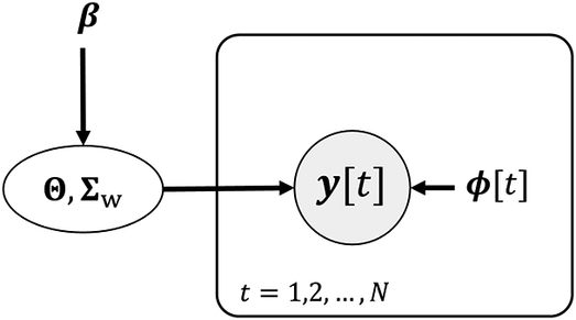
 as illustrated in the Bayesian network in Figure 2.
Bayesian network of the VAR model.
The likelihood of the complete time-series from the
$ {n}_a+1 $
 observation to the
$ {N}^{\mathrm{th}} $
observation to the
$ {N}^{\mathrm{th}} $
 observation,
$ {\boldsymbol{Y}}_{\tau } $
observation,
$ {\boldsymbol{Y}}_{\tau } $
 , is obtained by assuming conditional independence of the observations given the parameters:

By Bayes’ theorem (Murphy, Reference Murphy2012, p. 29), the joint posterior distribution of the parameters is then:

where the dependence on the hyperparameter
$ \boldsymbol{\beta} $
 is implicitly assumed, and the denominator is the marginal likelihood acting as a normalizing constant.
Calculating the joint posterior in Equation (11) is often not feasible, and simulation-based methods are typically employed. Under the assumption of conjugate priors, where the product of the prior and the likelihood belongs to the same family as the posterior, analytical expressions for the posterior can be obtained, which simplifies the inference process (Gelman, Reference Gelman2013, p. 36). For this, it is assumed that the likelihood
$ p\left({\boldsymbol{Y}}_{\tau}\;|\;\boldsymbol{\Theta}, {\boldsymbol{\Sigma}}_w,\boldsymbol{\Phi} \right) $
 and the prior
$ p\left(\boldsymbol{\Theta}\;|\;{\boldsymbol{\Sigma}}_w\right) $
and the prior
$ p\left(\boldsymbol{\Theta}\;|\;{\boldsymbol{\Sigma}}_w\right) $
 are Gaussian, each modeled using the Matrix Normal (
$ \mathcal{M}\mathcal{N} $
are Gaussian, each modeled using the Matrix Normal (
$ \mathcal{M}\mathcal{N} $
 ) distribution, and that the prior
$ p\left({\boldsymbol{\Sigma}}_w\right) $
) distribution, and that the prior
$ p\left({\boldsymbol{\Sigma}}_w\right) $
 is Inverse-Wishart (
$ \mathcal{I}\mathcal{W} $
is Inverse-Wishart (
$ \mathcal{I}\mathcal{W} $
 ) as follows:


where
$ \boldsymbol{I}\in {\unicode{x211D}}^{\tau \times \tau } $
 is the identity matrix, the mean
$ \boldsymbol{\mu} \in {\unicode{x211D}}^{m\times d} $
is the identity matrix, the mean
$ \boldsymbol{\mu} \in {\unicode{x211D}}^{m\times d} $
 and the covariance
$ \boldsymbol{V}\in {\unicode{x211D}}^{d\times d} $
and the covariance
$ \boldsymbol{V}\in {\unicode{x211D}}^{d\times d} $
 are the hyperparameters of the prior on
$ \boldsymbol{\Theta} $
are the hyperparameters of the prior on
$ \boldsymbol{\Theta} $
 , and the scale matrix
$ \boldsymbol{\Psi} \in {\unicode{x211D}}^{m\times m} $
, and the scale matrix
$ \boldsymbol{\Psi} \in {\unicode{x211D}}^{m\times m} $
 and degrees of freedom
$ \nu \in \unicode{x211D} $
and degrees of freedom
$ \nu \in \unicode{x211D} $
 are the hyperparameters of the prior on
$ {\boldsymbol{\Sigma}}_w $
are the hyperparameters of the prior on
$ {\boldsymbol{\Sigma}}_w $
 . With this, the prior hyperparameter
$ \boldsymbol{\beta} $
. With this, the prior hyperparameter
$ \boldsymbol{\beta} $
 in Figure 2 consists of
$ \left\{\boldsymbol{\mu}, \boldsymbol{V},\boldsymbol{\Psi}, \nu \right\} $
in Figure 2 consists of
$ \left\{\boldsymbol{\mu}, \boldsymbol{V},\boldsymbol{\Psi}, \nu \right\} $
 . Under these assumptions, conjugacy holds, and the posterior can be obtained analytically (Gelman, Reference Gelman2013, p. 584; Avendaño-Valencia, Reference Avendaño-Valencia2025). With the definitions in Equations. (12), (13), and (14), the posterior distribution in Equation (11) can be written as Gupta and Nagar (Reference Gupta and Nagar1999, Ch. 2–3):

Expanding the third term, the likelihood trace, gives:

Hence, the
$ \boldsymbol{\Theta} $
 -dependent part of Equation (15) can be grouped as:

Let

Then the
$ \boldsymbol{\Theta} $
 -dependent part can be expressed as:

Substituting this into Equation (15) and grouping the
$ \boldsymbol{\Theta} $
 -dependent and
$ \boldsymbol{\Theta} $
-dependent and
$ \boldsymbol{\Theta} $
 -independent parts results in:

with updates


which constitute the posterior hyperparameters after the inference.
The posterior hyperparameters can be inferred in two ways. The first is the batch update, in which the prior hyperparameters are defined once, and all available observations are incorporated simultaneously, yielding the posterior hyperparameters in Equations (21)–(24). The second is the sequential update, where the posterior after each batch of data is reused as the prior when new observations arrive (Avendaño-Valencia, Reference Avendaño-Valencia2025). In practice, this means that each new segment of data contributes an incremental update to the hyperparameters, allowing the model to gradually refine its description of the underlying dynamics without revisiting past data. This recursive procedure is beneficial when data arrive incrementally. However, it implicitly assumes that all new observations are consistent with the underlying dynamics, which, in practice, may be violated due to transient deviations and non-stationary behavior. As a result, directly applying the recursive update in Equations (21)–(24) may lead to abrupt changes in the inferred hyperparameters. To mitigate this, a regularized update can be adopted, in which the posterior hyperparameters are combined with the previous prior through a weighted update governed by forgetting factors
$ {\eta}_{\Sigma},{\eta}_{\Theta}\in \left[0,1\right] $
 :
:


controlling the influence of newly observed data relative to previously inferred information (Prando et al., Reference Prando, Romeres and Chiuso2016; Søndergaard et al., Reference Søndergaard, Shaker and Nørregaard Jørgensen2024; Prasanthi et al., Reference Prasanthi, Shareef, Khalid and Selvaraj2025), which can be determined either heuristically as fixed weights or adaptively. Both the batch update and sequential update strategies rely on the same conjugate structure, ensuring analytical tractability.
Marginalizing
$ \boldsymbol{\Theta} $
 and
$ {\boldsymbol{\Sigma}}_w $
and
$ {\boldsymbol{\Sigma}}_w $
 .
.
The model parameters
$ \boldsymbol{\Theta} $
 and
$ {\boldsymbol{\Sigma}}_w $
and
$ {\boldsymbol{\Sigma}}_w $
 are represented as posterior distributions because they are treated as random variables. Further analysis often involves expectations with respect to these posteriors, which in general are approximated by sampling-based methods, but this can be computationally inefficient. In this case of conjugacy, however, both
$ \boldsymbol{\Theta} $
are represented as posterior distributions because they are treated as random variables. Further analysis often involves expectations with respect to these posteriors, which in general are approximated by sampling-based methods, but this can be computationally inefficient. In this case of conjugacy, however, both
$ \boldsymbol{\Theta} $
 and
$ {\boldsymbol{\Sigma}}_w $
and
$ {\boldsymbol{\Sigma}}_w $
 can be marginalized analytically, yielding closed-form expressions for the marginal likelihood and avoiding the need for sampling.
Starting from the joint model in Equations (12)–(14), the first step is to marginalize
$ \boldsymbol{\Theta} $
 , resulting in the partly marginalized likelihood of
$ {\boldsymbol{Y}}_{\tau } $
, resulting in the partly marginalized likelihood of
$ {\boldsymbol{Y}}_{\tau } $
 :
:

In its vectorized form, this is similar to a standard Gaussian model
$ \boldsymbol{y}=\boldsymbol{Ax}+\boldsymbol{b} $
 in Murphy (Reference Murphy2012, p. 119), in which:


which is equivalent to Equation (29) with the following:

Following the definition in Murphy (Reference Murphy2012, p. 120), the partly marginalized likelihood of
$ {\boldsymbol{Y}}_{\tau } $
 can be expressed as:

and by following the Kronecker product of ordinary products (Harville, Reference Harville2006, p. 341), part of the covariance can be simplified:

so the complete covariance in Equation (33) simplifies into:

Reshaping back to Matrix–Normal form (Harville, Reference Harville2006, p. 345) yields:

which is Equation (29) and expresses the partly marginalized likelihood of
$ {\boldsymbol{Y}}_{\tau } $
 given
$ {\boldsymbol{\Sigma}}_w $
given
$ {\boldsymbol{\Sigma}}_w $
 and
$ \boldsymbol{\Phi} $
and
$ \boldsymbol{\Phi} $
 . To obtain the complete marginalized likelihood of
$ {\boldsymbol{Y}}_{\tau } $
. To obtain the complete marginalized likelihood of
$ {\boldsymbol{Y}}_{\tau } $
 , the innovation covariance
$ {\boldsymbol{\Sigma}}_w $
, the innovation covariance
$ {\boldsymbol{\Sigma}}_w $
 can also be marginalized as:

From Equation (36), the partly marginalized likelihood is Matrix–Normal and the prior on
$ {\boldsymbol{\Sigma}}_w $
 is Inverse–Wishart as in Equation (14). In vectorized form, the partly marginalized likelihood corresponds to:

and, combined with the Inverse-Wishart prior, the joint distribution
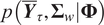
$ p\left({\overline{\boldsymbol{Y}}}_{\tau },{\boldsymbol{\Sigma}}_w|\boldsymbol{\Phi} \right) $
 belongs to the Normal-Inverse-Wishart (
$ \mathcal{N}\mathcal{I}\mathcal{W} $
belongs to the Normal-Inverse-Wishart (
$ \mathcal{N}\mathcal{I}\mathcal{W} $
 ) family (Murphy, Reference Murphy2012, pp. 132–133) expressed as:

Consequently, the complete marginalized likelihood in Equation (37) is a multivariate Student-
$ t $
 distribution for
$ {\overline{\boldsymbol{Y}}}_{\tau } $
distribution for
$ {\overline{\boldsymbol{Y}}}_{\tau } $
 (Murphy, Reference Murphy2012, p. 134). Reshaping back into matrix form gives a Matrix–Student–
$ t $
(Murphy, Reference Murphy2012, p. 134). Reshaping back into matrix form gives a Matrix–Student–
$ t $
 distribution:

The corresponding log marginal likelihood is written as Gupta and Nagar (Reference Gupta and Nagar1999, pp. 133–134):

where
$ {\Gamma}_m\left(\cdot \right) $
 denotes the multivariate gamma function and
$ \boldsymbol{S}={\boldsymbol{I}}_{\tau \times \tau }+{\boldsymbol{\Phi}}^{\top}\boldsymbol{V}\boldsymbol{\Phi } $
denotes the multivariate gamma function and
$ \boldsymbol{S}={\boldsymbol{I}}_{\tau \times \tau }+{\boldsymbol{\Phi}}^{\top}\boldsymbol{V}\boldsymbol{\Phi } $
 .
.
2.2. Multi-model approach
For systems operating under time-varying conditions, the assumption of stationarity for the discrete time-series
$ \boldsymbol{Y} $
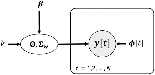
 is generally violated, as the statistical properties of the signal may change over time. A practical solution is to analyze the system on a local level by partitioning the full operation into operating regimes (Avendaño-Valencia, Reference Avendaño-Valencia2025), each approximately satisfying the stationarity assumption. Extending the Bayesian formulation introduced earlier (Figure 2), the VAR model can now be conditioned on the operating regime
$ k\in \left[1,2,\cdots, K\right] $
is generally violated, as the statistical properties of the signal may change over time. A practical solution is to analyze the system on a local level by partitioning the full operation into operating regimes (Avendaño-Valencia, Reference Avendaño-Valencia2025), each approximately satisfying the stationarity assumption. Extending the Bayesian formulation introduced earlier (Figure 2), the VAR model can now be conditioned on the operating regime
$ k\in \left[1,2,\cdots, K\right] $
 , where
$ K $
, where
$ K $
 is the total number of operating regimes, as illustrated in Figure 3.
Bayesian network of the VAR model conditioned on the operating regime
$ k $
 .
.
For each operating regime
$ k $
 , a separate set of prior hyperparameters
$ \left\{{\boldsymbol{\mu}}_k,{\boldsymbol{V}}_k,{\boldsymbol{\Psi}}_k,{\nu}_k\right\} $
, a separate set of prior hyperparameters
$ \left\{{\boldsymbol{\mu}}_k,{\boldsymbol{V}}_k,{\boldsymbol{\Psi}}_k,{\nu}_k\right\} $
 is introduced, such that the priors are conditioned on the operating regime
$ k $
is introduced, such that the priors are conditioned on the operating regime
$ k $
 :
:

Given a segment belonging to a regime
$ k $
 , the posterior hyperparameters
$ \left\{{\boldsymbol{\mu}}_k^{\left(\mathrm{post}\right)},{\boldsymbol{V}}_k^{\left(\mathrm{post}\right)},{\boldsymbol{\Psi}}_k^{\left(\mathrm{post}\right)},{\nu}_k^{\left(\mathrm{post}\right)}\right\} $
, the posterior hyperparameters
$ \left\{{\boldsymbol{\mu}}_k^{\left(\mathrm{post}\right)},{\boldsymbol{V}}_k^{\left(\mathrm{post}\right)},{\boldsymbol{\Psi}}_k^{\left(\mathrm{post}\right)},{\nu}_k^{\left(\mathrm{post}\right)}\right\} $
 follow the updates in Equations (21)–(24) using the regime-specific priors. However, when the regime
$ k $
follow the updates in Equations (21)–(24) using the regime-specific priors. However, when the regime
$ k $
 is unknown, it must be inferred, which is detailed in the following.
2.3. Definition of local references
The regime-specific hyperparameters
$ \left\{{\boldsymbol{\mu}}_k^{\left(\mathrm{post}\right)},{\boldsymbol{V}}_k^{\left(\mathrm{post}\right)},{\boldsymbol{\Psi}}_k^{\left(\mathrm{post}\right)},{\nu}_k^{\left(\mathrm{post}\right)}\right\} $
 , representing the local references, can be defined either using prior knowledge of the operating regimes (supervised setting) or inferred directly from the data (unsupervised setting).
In the supervised setting, prior knowledge of the operating regimes is used to partition the data accordingly. The regime-specific hyperparameters representing the local references are then inferred from the grouped data, resulting in a set of reference models associated with each predefined regime. In the unsupervised setting, the operating regimes are identified directly from the data based on the log marginal likelihood in Equation (41). Initially, prior hyperparameters are specified, and an initial batch of data is used to infer posterior hyperparameters, defining the first local reference. As new batches of data are observed sequentially, the log marginal likelihood of each batch is evaluated with respect to the existing reference models
$ k $
 as:
as:

where
$ \boldsymbol{S}={\boldsymbol{I}}_{\tau \times \tau }+{\boldsymbol{\Phi}}^{\top }{\boldsymbol{V}}_k\boldsymbol{\Phi} $
 . Among the existing operating regimes, the one that maximizes the log marginal likelihood is selected as the most probable explanation of the new data batch:

If the likelihood is sufficiently high, the corresponding reference model of the operating regime
$ \hat{c} $
 is updated using the new data. Conversely, if the likelihood is low, the data are not well explained by the existing references, and a new local reference is initialized based on the inferred posterior hyperparameters of that batch. This sequential procedure is repeated over the available data, resulting in a set of local references learned directly from the data without requiring prior knowledge of regime boundaries or the number of regimes.
2.3.1. Detection of anomalies
A large value of the log marginal likelihood given a segment
$ {\boldsymbol{Y}}_t $
 indicates that the new data segment is highly consistent with the statistical structure represented by regime
$ \hat{c} $
indicates that the new data segment is highly consistent with the statistical structure represented by regime
$ \hat{c} $
 . Conversely, low values indicate that the observed data are poorly explained by the corresponding regime-specific model. This may indicate that the segment
$ {\boldsymbol{Y}}_t $
. Conversely, low values indicate that the observed data are poorly explained by the corresponding regime-specific model. This may indicate that the segment
$ {\boldsymbol{Y}}_t $
 corresponds to an operating condition that deviates significantly from the defined operating regimes and thereby the regime-specific dynamics. However, individual segments that are poorly explained by the local references may arise due to transient deviations or isolated outliers. To improve robustness against such effects, the anomaly assessment is not performed on individual segments, but rather based on an accumulated statistic over a sliding window of length
$ J $
corresponds to an operating condition that deviates significantly from the defined operating regimes and thereby the regime-specific dynamics. However, individual segments that are poorly explained by the local references may arise due to transient deviations or isolated outliers. To improve robustness against such effects, the anomaly assessment is not performed on individual segments, but rather based on an accumulated statistic over a sliding window of length
$ J $
 segments. Specifically, the anomaly detection statistic is defined as:
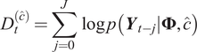
which represents the cumulative log marginal likelihood of the most recent observations under regime
$ \hat{c} $
 . Low values of
$ {D}_t^{\left(\hat{c}\right)} $
. Low values of
$ {D}_t^{\left(\hat{c}\right)} $
 indicate that the recent sequence of observations is unlikely under the reference model, and therefore suggest a persistent deviation from the learned regime behavior. Based on this, the structural condition is assessed as:


where
$ {\vartheta}_{\hat{c}} $
 denotes a regime-dependent threshold. The threshold
$ {\vartheta}_c $
denotes a regime-dependent threshold. The threshold
$ {\vartheta}_c $
 is determined empirically from the training data by estimating the distribution of
$ {D}_t^{(c)} $
is determined empirically from the training data by estimating the distribution of
$ {D}_t^{(c)} $
 under each regime and selecting a lower-tail quantile. This provides a statistically interpretable criterion for anomaly detection, ensuring that the decision is consistent with the variability observed within each regime. This accumulated statistic can be interpreted as a measure of joint evidence over multiple observations, reducing sensitivity to isolated outliers while emphasizing persistent deviations.
As an extension to the above formulation, the evolution of the accumulated statistic
$ {D}_t^{\left(\hat{c}\right)} $
 over time can be monitored to identify gradual deviations from the reference condition. A consistent downward trend in
$ {D}_t^{\left(\hat{c}\right)} $
over time can be monitored to identify gradual deviations from the reference condition. A consistent downward trend in
$ {D}_t^{\left(\hat{c}\right)} $
 indicates a progressive reduction in the log marginal likelihood, which may be interpreted as a gradual degradation of the system. This enables the framework to provide early-warning indicators of structural changes beyond binary anomaly detection.
3. Case study: SHM for a Crew Transfer Vessel
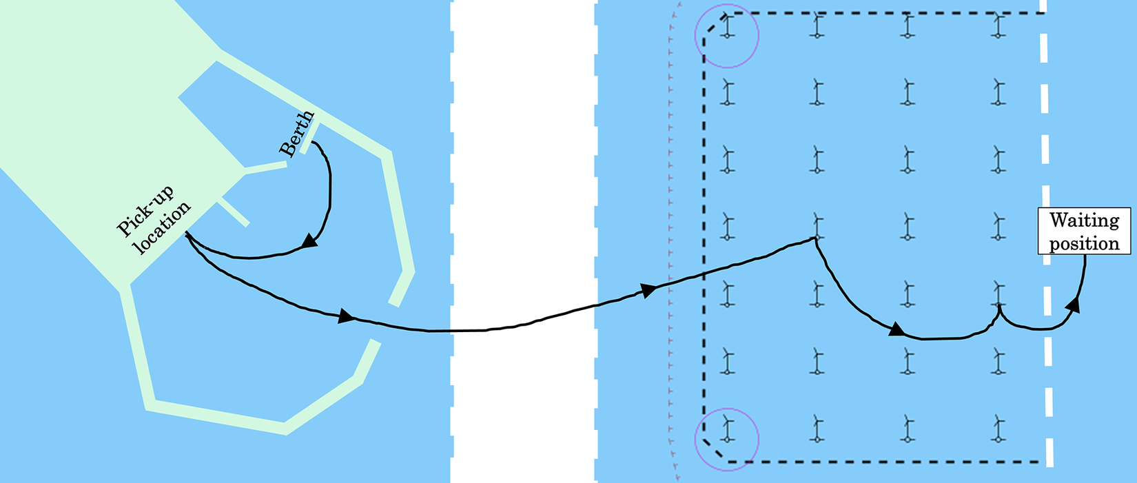
The proposed multi-model approach for anomaly detection under time-varying operating conditions is implemented and tested within a VBSHM framework for a gearbox on a CTV. The CTV operates between shore and offshore wind farms, transporting technicians and cargo to offshore wind turbines, where the operation is partly illustrated in Figure 4. A typical day begins with the CTV departing its berthing position to pick up personnel and equipment at a designated harbor location, and then transporting these to the wind farms. Once entering the farm, the procedure is to push the bow of the CTV against the turbine tower to enable a safe transfer of the technicians. Once all technicians are deployed to their assigned turbines, the CTV moves to a waiting position. Depending on the duration of the technicians’ tasks, the CTV either relocates them to other turbines or waits until the end of the day to pick them up. Finally, the CTV returns all personnel to the harbor and proceeds back to its berthing position. However, the safe transfer of technicians, relying on the CTV pushing its bow against the turbine tower, is often hindered by unfavorable weather conditions. Such conditions can lead to the cancellation of the entire day’s operation, increasing the pressure to maximize operation during favorable weather windows. As a result, this intensified operation places additional stress on critical structural components, particularly the gearboxes between the engines and propellers. To minimize the risk of unexpected breakdowns, implementing an SHM framework is feasible; however, this is significantly challenged by the highly time-varying operation of the CTV.
Example of operational pattern from berthing position, picking up technicians at a designated location, transit to offshore wind farm, push-on two turbines, and, lastly, entering a waiting position.
Following the multi-model framework, operational regimes must be identified. However, in the context of a CTV, regimes with stationary operational properties are not easily defined. This is due to the complex interplay between environmental and operational factors that the captain must continually navigate. As a result, human decision-making introduces an additional layer of uncertainty. A practical approximation is to divide the operation into its individual tasks, referred to as Operational modes, thereby following the multi-model’s supervised identification of regimes as detailed in Section 2.3. These modes can be readily defined through observation and are, from a structural dynamic perspective, assumed to each exert a unique influence on the gearboxes. In total, the CTV performs seven different tasks throughout a typical day of operation, resulting in seven operational modes:
-
1. At berth: The engines are either turned off or running idle. Mooring lines secure the berthing position.
-
2. Maneuvering harbor: The engines are running at variable RPM; however, at a considerably low level. The environmental influence is assumed to be negligible.
-
3. Pick-up: The CTV is pushing against a specially designed ladder at the designated pick-up location to keep a stationary position while the technicians are boarding. The engines are running at constant RPM to maintain a certain pushing force.
-
4. Transit: The engines are running close to maximum RPM to keep maximum speed. The ocean conditions can have a significant influence.
-
5. Maneuvering farm: Similar to the transit mode; however, the RPM and speed can fluctuate due to the maneuverability. Typically, the speed and RPM are lower than in the transit mode.
-
6. At turbine: The engines are running at a high RPM level to maintain a high pushing force on the turbine tower while technicians and cargo are transferred to the turbine. In addition, the ocean conditions can have a significant influence.
-
7. Waiting: Several of the engines are turned off or running idle, depending on the weather and ocean conditions, while the CTV drifts while waiting for the technicians to finish their tasks.
While assuming stationary operational properties for each mode is a coarse approximation—and the boundaries between modes are not sharply defined—this partitioning enables a practical implementation of the multi-model framework. This is further supported by the fact that the crew logs the start and end of each mode in a Daily Progress Report (DPR), resulting in a readily accessible partition.
With the operation partitioned into operational modes, the following details the data used for the multi-model framework and outlines the specific details of the multi-model.
3.1. Data acquisition
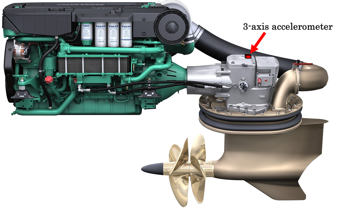
The CTV is equipped with four propulsion units, each consisting of a diesel engine, a gearbox, and a propeller set, as shown in Figure 5, where the propellers are facing forward. As the CTV is a catamaran, each hull contains two propulsion units. Accordingly, the data acquisition system measures the vibrational response of a single gearbox located in one of the hulls. The vibrational response of the gearbox is measured by a three-axis accelerometer mounted on top of the gearbox Figure 5. The accelerometer is oriented such that the x-axis corresponds to forward–backwards motion, the y-axis to lateral motion, and the z-axis to vertical motion. In this context, the gearbox is considered a coupled dynamical system, where the measured vibrational response arises from the interaction of multiple internal components, including gears, shafts, and bearings. The three-axis accelerometer therefore captures different projections of this coupled behavior, resulting in a multivariate signal.
Location of the accelerometer on one of the propulsion units.
For this preliminary study, where the proposed multi-model framework is tested, data collected over 1 month during summer, in which the vibrational response was measured, is used to establish the pool of references. During this month, 14 days of operation were cancelled, resulting in 17 days of operation where the vibrational response was measured. Subsequently, a small dataset including 4 days of operation is used to test the multi-model on a dataset without any structural changes.
Approximately 6 months later, repairs were carried out on both drive shafts between the engines and gearboxes, and new sets of propellers were installed. A small dataset collected after these repairs is therefore used to test the detectability of anomalies, although data capturing gradual structural degradation would have been preferable. However, the limited size of the post-repair dataset prevents it from being used as a reference condition. Furthermore, the available post-repair dataset represents a step change in the system condition rather than gradual degradation. While this is not fully representative of typical damage evolution, it provides a controlled change in system behavior that enables evaluation of the multi-model’s ability to detect deviations from the learned reference condition. The complete dataset is available through Zenodo (Drangsfeldt, Reference Drangsfeldt2026). The details of the data acquisition system and the dimensions of the datasets are detailed in Table 1.
Overview of the data acquisition
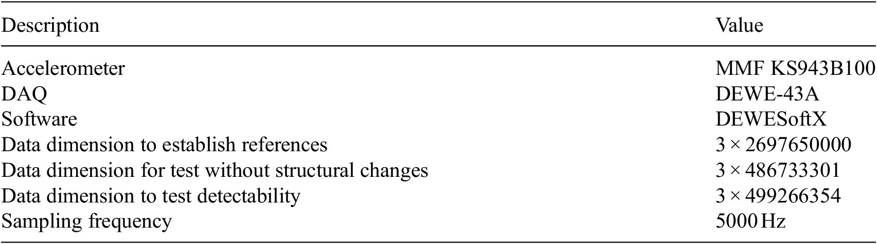
Table 1. Long description
The table consists of two columns: Description and Value.
* Row 1: Accelerometer is M M F K S 9 4 3 B 1 0 0.
* Row 2: D A Q is D E W E dash 4 3 A.
* Row 3: Software is D E W E Soft X.
* Row 4: Data dimension to establish references is 3 times 2,697,650,000.
* Row 5: Data dimension for test without structural changes is 3 times 486,733,301.
* Row 6: Data dimension to test detectability is 3 times 499,266,354.
* Row 7: Sampling frequency is 5000 H z.
3.2. Comparison to a traditional SHM approach
As a benchmark representing a traditional SHM approach, one of the methodologies presented in Drangsfeldt and Avendaño-Valencia (Reference Drangsfeldt and Avendaño-Valencia2024) is adopted. This approach is based on using the parameters of VAR models as DSFs, implicit mitigation of EOV through PCA, and the squared Mahalanobis distance as a measure of correspondence to a global reference model. This benchmark serves as a reference for evaluating the limitations of global reference-based approaches under discrete and varying operational conditions, where regime-dependent variability is not explicitly accounted for.
First, the dataset used to establish the reference model is segmented into intervals of 5-second duration, resulting in
$ 107906 $
 segments, each represented as
$ \boldsymbol{Y}\in {\unicode{x211D}}^{3\times 25000} $
segments, each represented as
$ \boldsymbol{Y}\in {\unicode{x211D}}^{3\times 25000} $
 . A VAR model is fitted to each segment using Least Squares estimation as defined in Equations (5) and (7). The estimated AR parameters,
$ \boldsymbol{\Theta} $
. A VAR model is fitted to each segment using Least Squares estimation as defined in Equations (5) and (7). The estimated AR parameters,
$ \boldsymbol{\Theta} $
 , constitute the DSFs. The complete set of DSFs from all
$ 107906 $
, constitute the DSFs. The complete set of DSFs from all
$ 107906 $
 segments defines the global reference:

where
$ \mathcal{M} $
 represents the global reference state of the gearbox. Following the PCA procedure for implicit mitigation of EOV, each
$ \boldsymbol{\Theta} $
represents the global reference state of the gearbox. Following the PCA procedure for implicit mitigation of EOV, each
$ \boldsymbol{\Theta} $
 is first vectorized, denoted as
$ \overline{\boldsymbol{\theta}}=\mathrm{vec}\left(\boldsymbol{\Theta} \right) $
is first vectorized, denoted as
$ \overline{\boldsymbol{\theta}}=\mathrm{vec}\left(\boldsymbol{\Theta} \right) $
 , and subsequently normalized to obtain
$ \tilde{\boldsymbol{\theta}} $
, and subsequently normalized to obtain
$ \tilde{\boldsymbol{\theta}} $
 , using the mean and standard deviation estimated from the vectorized reference
$ \overline{\mathcal{M}} $
, using the mean and standard deviation estimated from the vectorized reference
$ \overline{\mathcal{M}} $
 . A Singular Value Decomposition is then applied to the vectorized, normalized reference:

where
$ \boldsymbol{P} $
 denotes the right singular vector matrix. This is used to transform each incoming, vectorized, and normalized AR parameter vector
$ \tilde{\boldsymbol{\theta}} $
denotes the right singular vector matrix. This is used to transform each incoming, vectorized, and normalized AR parameter vector
$ \tilde{\boldsymbol{\theta}} $
 into Principal Component (PC) space:

As proposed in Drangsfeldt and Avendaño-Valencia (Reference Drangsfeldt and Avendaño-Valencia2024), the PCs accounting for up to 90% of the accumulated variance are discarded, as they are assumed to primarily represent EOV. Similarly, PCs beyond 99% of the accumulated variance are removed to reduce the influence of noise. Finally, the squared Mahalanobis distance is used to assess whether an incoming observation corresponds to an outlier relative to the transformed global reference:

where
$ {\mathcal{M}}^{\star } $
 denotes the global reference projected into the reduced PC space. Then, by treating every 5-second segment as an incoming observation, the squared Mahalanobis distance is shown in Figure 6. Under the assumption that the retained PCs are approximately Gaussian, the squared Mahalanobis distance follows a chi-square distribution,
$ {d}^2\sim {\chi}_r^2 $
denotes the global reference projected into the reduced PC space. Then, by treating every 5-second segment as an incoming observation, the squared Mahalanobis distance is shown in Figure 6. Under the assumption that the retained PCs are approximately Gaussian, the squared Mahalanobis distance follows a chi-square distribution,
$ {d}^2\sim {\chi}_r^2 $
 , with degrees of freedom equal to the number of retained PCs. Therefore, outlier (anomaly) detection is performed as:


where
$ r $
 denotes the number of retained PCs, and
$ {\chi}_{r,1-\alpha}^2 $
denotes the number of retained PCs, and
$ {\chi}_{r,1-\alpha}^2 $
 is the
$ \left(1-\alpha \right) $
is the
$ \left(1-\alpha \right) $
 -quantile of the chi-square distribution. The horizontal threshold shown in Figure 6 represents a confidence level of 99%, corresponding to
$ \alpha =0.01 $
-quantile of the chi-square distribution. The horizontal threshold shown in Figure 6 represents a confidence level of 99%, corresponding to
$ \alpha =0.01 $
 .
.
The squared Mahalanobis distance for each 5-second segment follows the benchmark approach for anomaly detection.
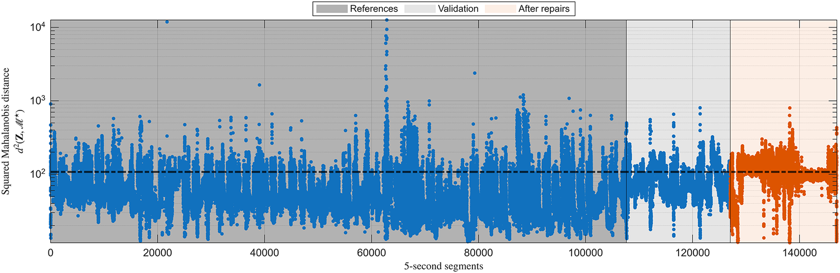
Figure 6. Long description
A scatter plot with a logarithmic Y axis labeled Squared Mahalanobis distance d squared (Z, M super asterisk) ranging from 10 super 1 to 10 super 4. The X axis is labeled 5-second segments ranging from 0 to 150,000. A horizontal dashed black line represents a threshold at approximately 10 super 2.
* The first phase, References, is shaded dark gray and spans from segment 0 to approximately 107,000. It contains blue data points mostly clustered below the threshold, with several vertical spikes reaching 10 super 3 and one extreme outlier near 10 super 4 at segment 62,000.
* The second phase, Validation, is shaded light gray from segment 107,000 to 127,000. It continues with blue data points showing similar density and variance to the reference phase.
* The third phase, After repairs, is shaded light orange from segment 127,000 to the end. The data points in this section are colored orange. The variance appears slightly reduced compared to previous phases, with most points tightly clustered around the threshold line and fewer high-magnitude outliers.
As a result, 46.8% of the 5-second segments from the dataset acquired after the repairs are classified as anomalies. However, 12.6% of the segments from the dataset prior to the repairs are also classified as anomalies, indicating a relatively high false positive rate for the global reference-based approach adopted from Drangsfeldt and Avendaño-Valencia (Reference Drangsfeldt and Avendaño-Valencia2024).
3.3. Establishing the references of the multi-model
The first step of the proposed multi-model framework in the supervised setting is to establish an accurate representation of the posterior hyperparameters for each regime. As detailed in Section 2.1.1, this can be achieved either through a batch update or a sequential update process. A batch update, however, presents two main challenges. First, the matrix inversion required in Equation (21) becomes computationally expensive when the batch is large, since the regression matrix
$ \boldsymbol{\Phi} $
 grows proportionally with the data length. Second, maintaining the stationarity assumption for
$ \boldsymbol{Y} $
grows proportionally with the data length. Second, maintaining the stationarity assumption for
$ \boldsymbol{Y} $
 becomes increasingly difficult when a long data segment is used. In contrast, a sequential update is less computationally demanding because it processes smaller segments iteratively. However, the iterative procedure can be extensive, and some segments may continue to violate the stationarity assumption. To address the challenge of possible non-stationarities in the data obtained, a regularized updating process is adopted, as detailed in Section 2.1.1. This approach introduces forgetting factors to control the influence of newly observed data relative to previously inferred information, thereby mitigating the effect of short data segments that may violate the stationarity assumption.
First, the dataset used to establish the local references is segmented into segments of 5 seconds. This results in
$ \boldsymbol{Y}\in {\unicode{x211D}}^{3\times 25000} $
 , where
$ \boldsymbol{Y} $
, where
$ \boldsymbol{Y} $
 is associated with its corresponding operational mode according to the DPR. Then, flat priors for each operational mode are adopted initially, and then updated sequentially using the segmented
$ \boldsymbol{Y} $
is associated with its corresponding operational mode according to the DPR. Then, flat priors for each operational mode are adopted initially, and then updated sequentially using the segmented
$ \boldsymbol{Y} $
 . These prior hyperparameters are therefore defined such that the corresponding prior distributions are flat:


The forgetting factors for the regularized updating process are selected as 0.01 and 0.05, respectively, reflecting a balance between responsiveness to evolving system dynamics and robustness to transient deviations and noise. These values were chosen to ensure stable convergence of the inferred hyperparameters while maintaining sufficient adaptability to changes in the observed behavior. The first part of the updating strategy is shown in Figure 7, displaying the first four coefficients in
$ \boldsymbol{\Theta} $
 for operational mode 3. The underlying grey Credible Interval (CI) and mean labelled as No updating correspond to the case where every 5-second segment in
$ \boldsymbol{Y} $
for operational mode 3. The underlying grey Credible Interval (CI) and mean labelled as No updating correspond to the case where every 5-second segment in
$ \boldsymbol{Y} $
 follows the batch updating strategy where no updating is performed. In this case, the prior hyperparameter
$ {\boldsymbol{\mu}}_k $
follows the batch updating strategy where no updating is performed. In this case, the prior hyperparameter
$ {\boldsymbol{\mu}}_k $
 is estimated using Least Squares estimation and the prior hyperparameter
$ {\boldsymbol{V}}_k $
is estimated using Least Squares estimation and the prior hyperparameter
$ {\boldsymbol{V}}_k $
 is set to
$ 0.001\cdot {\boldsymbol{I}}_{d\times d} $
is set to
$ 0.001\cdot {\boldsymbol{I}}_{d\times d} $
 . Additionally, prior hyperparameters
$ {\boldsymbol{\Psi}}_k $
. Additionally, prior hyperparameters
$ {\boldsymbol{\Psi}}_k $
 and
$ {\nu}_k $
and
$ {\nu}_k $
 are set as in Equation (54). With the defined forgetting factors, the posterior gradually adapts to new observations while avoiding overfitting to minor variations observed when every 5-second segment follows the batch updating strategy.
Example of the updating strategy for Mode 3 after having observed 144 sets of 5 seconds duration, all belonging to Mode 3.
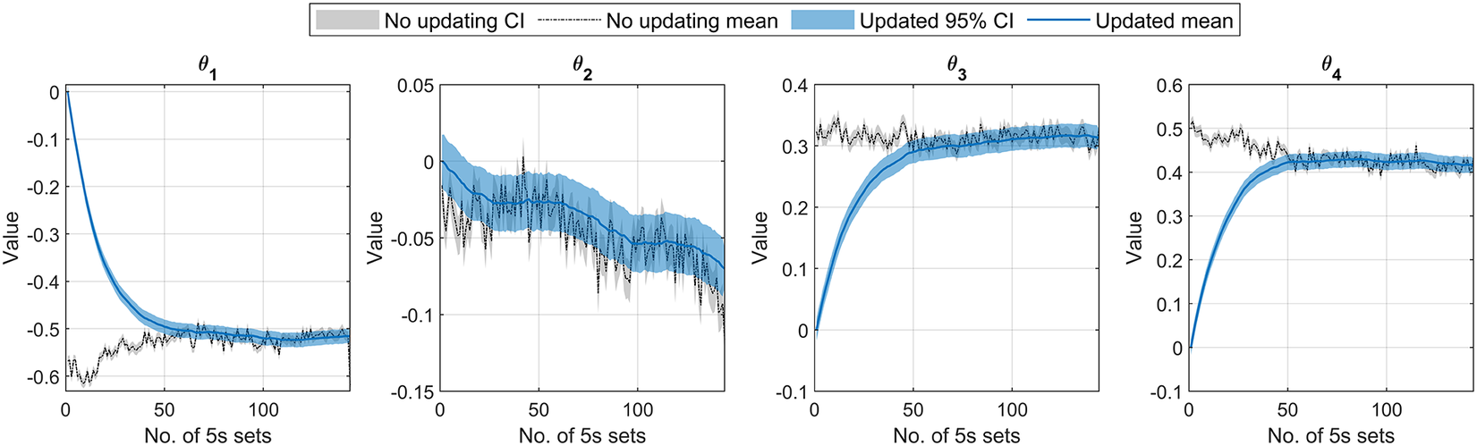
Figure 7. Long description
A legend at the top identifies four data series: No updating C I (gray shaded area), No updating mean (black dotted line), Updated 95% C I (blue shaded area), and Updated mean (solid blue line). All four panels share an x-axis labeled No. of 5 s sets ranging from 0 to 144 and a y-axis labeled Value.
* Panel 1 (theta sub 1): The updated mean shows a steep exponential decay from 0 to a steady state of negative 0.5. The non-updated mean fluctuates around negative 0.55 with a wider gray C I.
* Panel 2 (theta sub 2): The updated mean shows a gradual linear decrease from 0 to negative 0.07. The non-updated mean shows high-frequency oscillations between 0 and negative 0.1.
* Panel 3 (theta sub 3): The updated mean shows an asymptotic increase from 0, leveling off at 0.32. The non-updated mean is relatively flat, fluctuating around 0.32 with significant noise.
* Panel 4 (theta sub 4): The updated mean shows an asymptotic increase from 0, leveling off at 0.42. The non-updated mean fluctuates around 0.45 with a gray C I that narrows slightly over time.
Lastly, the model order
$ {n}_a $
 is selected based on a systematic model selection procedure. Specifically, Least Squares estimations are performed on multiple data segments representing different operational modes, and the resulting models are evaluated using both the Residual Sum of Squares over the Series Sum of Squares (RSS/SSS) and the Bayesian Information Criterion (BIC). These criteria provide a balance between model fit and model complexity. Based on this analysis, a model order of
$ {n}_a=20 $
is selected based on a systematic model selection procedure. Specifically, Least Squares estimations are performed on multiple data segments representing different operational modes, and the resulting models are evaluated using both the Residual Sum of Squares over the Series Sum of Squares (RSS/SSS) and the Bayesian Information Criterion (BIC). These criteria provide a balance between model fit and model complexity. Based on this analysis, a model order of
$ {n}_a=20 $
 was found to provide a suitable trade-off and is therefore adopted for all operational modes.
3.4. Procedure of the multi-model
After establishing the posterior hyperparameters for each regime, which serve as local references, the procedure follows Equation (44) for regime predictions among the existing reference models, where every 5-second segment is treated as a new observation. Following Equation (44), the log marginal likelihood of observing every 5-second segment given each reference operational mode is calculated, and determines the classified operational modes. The maximum log marginal likelihood for every 5-second segment is shown in Figure 8 with its classified operational mode. Here, every 5-second segment in both the dataset used for establishing the references and for testing without structural changes is treated as a new observation. It is observed that, despite significant variability for some of the operational modes, the 5-second segments in the testing dataset align well with the 5-second segments in the dataset used to define the references.
Maximum log marginal likelihood of observing every 5-second segment with the associated predicted operational mode,
$ p\left({\boldsymbol{Y}}_{\tau}^{(u)}|\boldsymbol{\Phi}, \hat{c}\right) $
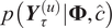 , where every segment in both the reference and test dataset is treated as a new observation.
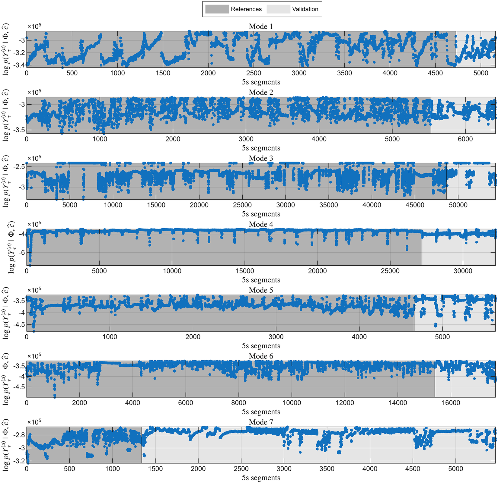
Figure 8. Long description
A multi-panel figure with seven horizontal scatter plots. A legend at the top indicates dark gray shading for References and light gray shading for Validation. Each plot shares a common y-axis label: log p ( Y sub tau super (u) | Phi, c-hat) times 10 super 5, and a common x-axis label: 5 s segments.
* Mode 1: Data points fluctuate between negative 3.4 and negative 3.0. The reference region ends near segment 4700.
* Mode 2: Data shows a dense band between negative 3.5 and negative 3.0, extending to approximately 6500 segments.
* Mode 3: Likelihood values are concentrated between negative 3.0 and negative 2.5, with significant downward spikes. The reference region ends at segment 45000.
* Mode 4: A very stable horizontal trend near negative 4.0 with occasional sharp downward drops. The reference region ends at segment 27000.
* Mode 5: Data fluctuates around negative 3.7, with the reference region concluding at segment 4700.
* Mode 6: Values are mostly stable near negative 3.5 with downward noise. The reference region ends at segment 15000.
* Mode 7: Shows a distinct shift in likelihood levels around segment 1400, where the reference region ends and validation begins, with values rising from negative 3.0 toward negative 2.8.
Finally, the maximum log marginal likelihood for every segment, as shown in Figure 8, also serves as an anomaly indicator as detailed in Section 2.3.1. This is elaborated and analyzed in the following section.
4. Detection of structural changes
As a continuous extension of the previous analysis, which was shown in Figure 8, the data reserved for testing the multi-model’s ability to detect anomalies is used. Although this is a small dataset that does not encompass all the variability the CTV encounters, it enables a preliminary test of the multi-model framework. Every 5-second set of
$ \boldsymbol{Y} $
 from the dataset reserved for testing the detectability is treated as a new observation, and the associated operational mode is predicted based on the maximum log marginal likelihood as in Equation (44). The maximum log marginal likelihood for every 5-second segment is shown in Figure 9 as an extension to Figure 8.
Test of the multi-model’s detectability.
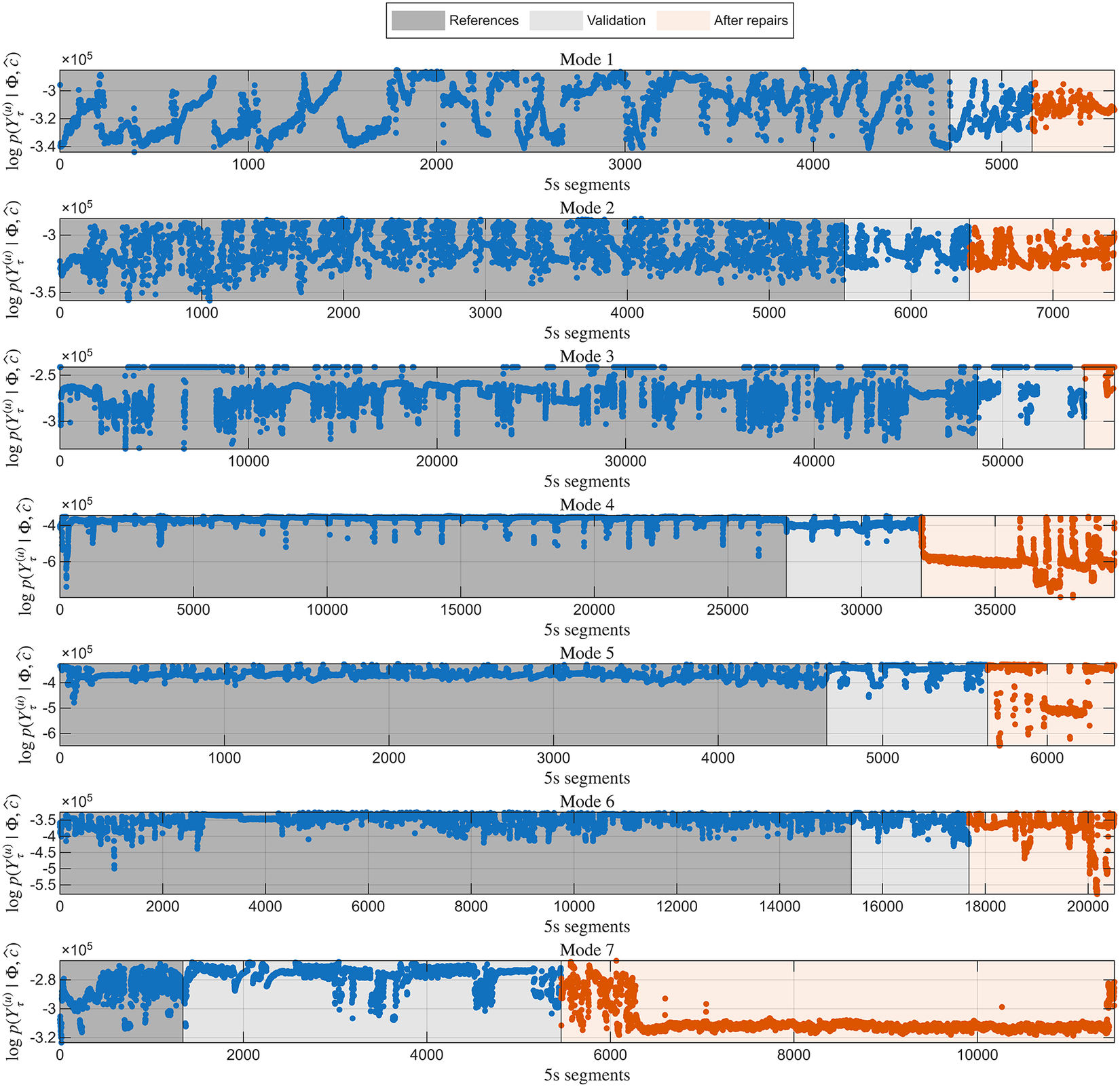
Figure 9. Long description
A multi-panel figure containing seven horizontal line graphs labeled Mode 1 through Mode 7.
At the top, a shared legend identifies three background regions: dark gray for References, light gray for Validation, and light orange for After repairs.
Each graph shares the same Y-axis label: log p (Y sub tau super u | Phi, c-hat ) times 10 super 5. The X-axis for all graphs is labeled 5s segments.
* Mode 1: Data points fluctuate between -3.4 and -3.0. The After repairs phase begins around segment 5200 with orange points showing a slight upward trend.
* Mode 2: Data is densely clustered between -3.5 and -3.0. The After repairs phase starts at segment 6400.
* Mode 3: Shows a plateau near -2.5 with frequent downward spikes to -3.2. The After repairs phase begins at segment 55000.
* Mode 4: Features a stable line near -4.0 with sharp downward spikes. At segment 32000, the After repairs phase shows a significant drop to -6.0 followed by high volatility.
* Mode 5: Data is stable near -3.0. The After repairs phase starts at segment 5600, showing a sudden drop and scattered points between -4.0 and -6.0.
* Mode 6: Data fluctuates near -3.5. The After repairs phase begins at segment 17800 with orange points showing increased downward variance.
* Mode 7: The References phase is short, ending at segment 1200. The Validation phase extends to segment 5400. The After repairs phase shows a sharp drop from -2.8 to -3.1, stabilizing at the lower value through segment 11000.
Despite the variability previously noted in Figure 8, deviations following the repairs are primarily observed for operational modes 4 and 7, and slightly for modes 5 and 6. The most pronounced deviations occur in mode 4, which aligns well with the physical interpretation of the structural behavior. Mode 4 corresponds to the transit period between the harbor and the wind farm, during which the engines operate at high RPM, and the CTV is near its maximum speed, placing substantial loads on the gearboxes. Consequently, (i) most of the available data contributes to refining the understanding of the local reference, and (ii) the operation within this mode is assumed to be the most consistent among all modes.
A slightly decreased tendency is observed for modes 5 and 6; however, without prior knowledge of when the structural changes occurred, this is nearly impossible to interpret conclusively. Furthermore, considerable variability is observed for modes 1, 2, and 3, which obscures any clear separation between the periods before and after the repairs. These modes comprise operation within the harbor, where the operational types may not be consistent. However, in mode 3, where the CTV pushes against the specially designed ladder used for technician transfer, the gearboxes are expected to experience a higher level of excitation—sufficient for the repairs to be detectable. Although both mode 3 and mode 6 involve push-on operations, the variability observed in mode 3 is interpreted as arising primarily from the inherent variability of this operating condition, rather than from model uncertainty, since such variability is not present in mode 6.
Following the accumulated statistic approach for anomaly detection detailed in Section 2.3.1, the detection threshold is defined as the 1% lower-tail quantile of the accumulated statistic, estimated from the data reserved for establishing the references for each operational mode. The sliding window length,
$ J $
 in Equation (45), is set to 60 segments. This corresponds to a conservative detection criterion, where only persistently unlikely observations are classified as anomalies. The resulting anomaly detection is illustrated in Figure 10. It is observed that the approach achieves the highest detection performance for operational modes 4 and 7. For mode 4, a True Negative Rate (TNR) and True Positive Rate (TPR) of 95.5% and 99.4% are obtained, respectively. Similarly, for mode 7, TNR and TPR values of 99.7% and 85.1% are achieved. However, for modes 5 and 6—both associated with operation outside the harbor area—the performance is reduced. For mode 5, the TNR and TPR are 98.4% and 48.1%, respectively, while for mode 6, the corresponding values are 98.3% and 14.9%. Lastly, for modes 1, 2, and 3—all associated with operation inside the harbor area—the TNR is 98.85%, 98.92%, and 98.88%, respectively, while the TPR is 0% for all three modes.
Test of the multi-model’s detectability of anomalies based on accumulated statistics.
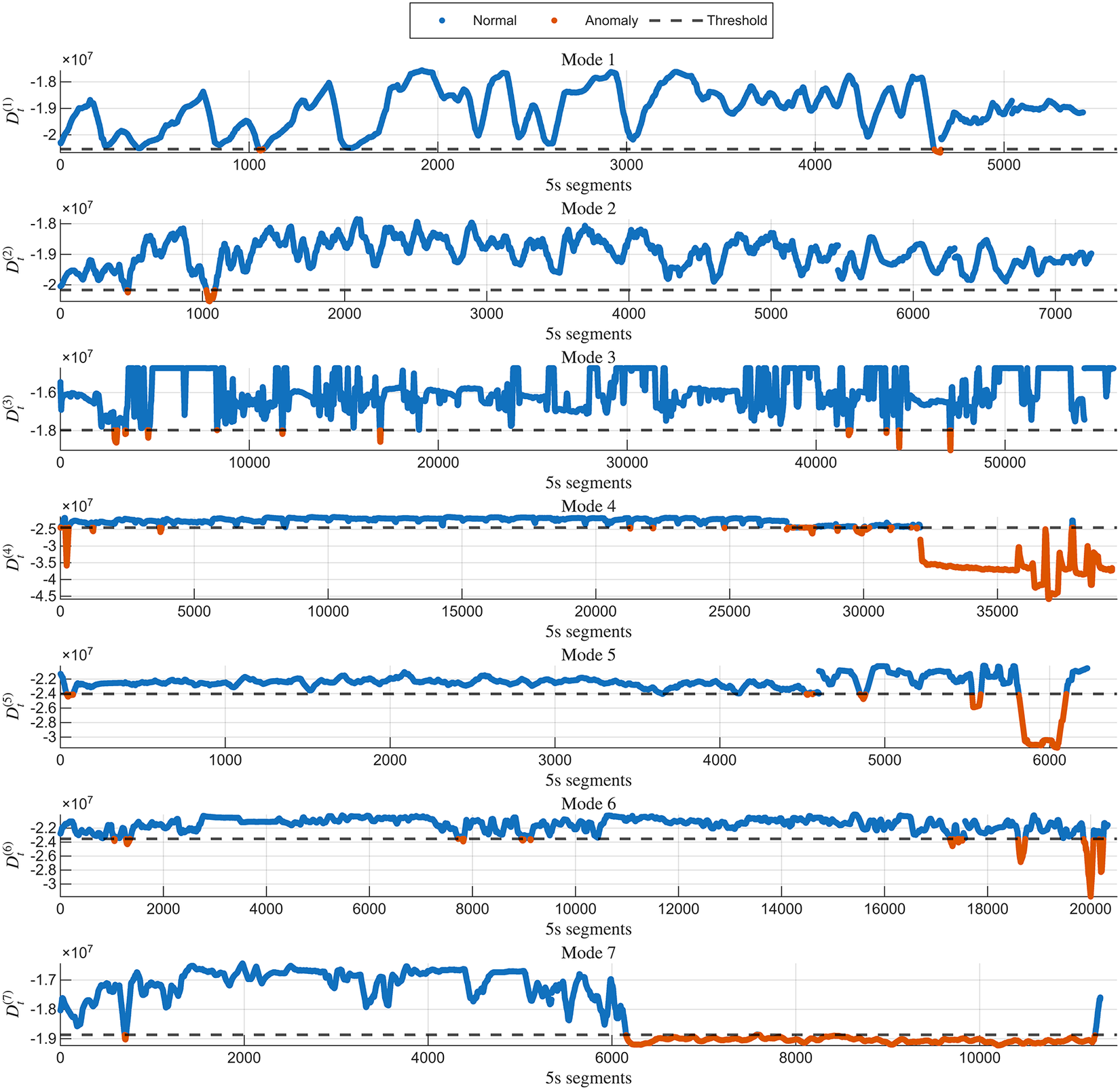
Figure 10. Long description
A vertical stack of seven line graphs labeled Mode 1 through Mode 7. A shared legend at the top identifies blue dots as Normal, orange dots as Anomaly, and a horizontal dashed line as the Threshold.
All panels share a common Y-axis format representing D sub t super (n) multiplied by 10 super 7, and an X-axis labeled 5 s segments.
* Mode 1: Fluctuating blue line between -2.1 and -1.75. A single orange anomaly point appears near segment 4600 where the line dips below the dashed threshold.
* Mode 2: Highly oscillatory blue line. Three distinct orange anomaly clusters appear near segments 1000, 4000, and 6200 where the troughs cross the threshold.
* Mode 3: A square-wave-like blue signal. Frequent orange anomaly spikes drop below the -1.8 threshold across the entire 50000 segment range.
* Mode 4: Mostly stable blue line near -2.3. A significant shift occurs after segment 32000 where the line turns orange and drops sharply to -3.5, staying below the threshold.
* Mode 5: Blue line with minor fluctuations until segment 5500, where it turns orange and plunges to a deep trough at -3.0.
* Mode 6: Blue line with intermittent orange anomaly dips below the -2.35 threshold, particularly concentrated after segment 17000.
* Mode 7: Blue line remains above the -1.88 threshold until segment 6200, after which the entire signal turns orange and remains consistently below the threshold for the remainder of the timeline.
5. Discussion
A Bayesian multi-model framework for VBSHM was proposed and tested using the measured vibrational response from a gearbox in the propulsion system of a CTV. The early development stage of the SHM system—combined with confidentiality constraints—highlights practical limitations, including sparse data, the lack of measured RPM, and a lack of detailed gearbox specifications. As a result, the detection of anomalies, presumably caused by structural changes, is not perfect. However, some interesting aspects are discussed in the following.
As a benchmark for the proposed framework, a traditional SHM approach was adopted in which the AR parameters of VAR models are used as DSFs to construct a global reference model. The influence of EOV was implicitly mitigated using PCA, under the assumption that the dominant variance is primarily driven by EOV. Following this approach, anomalies were detected; however, the TPR was limited to 46.8%. In addition, the detection threshold was defined based on the squared Mahalanobis distance under the assumption that the retained PCs follow a Gaussian distribution, leading to a chi-square-based threshold. However, when treating the system as a single global reference despite the presence of discrete operational regimes, this Gaussian assumption becomes overly restrictive. As a result, the threshold does not achieve the intended statistical coverage, as a significant portion of the reference data is incorrectly classified as anomalies. These observations indicate that global reference-based approaches are limited in their ability to account for regime-dependent variability. This limitation is further highlighted by the proposed multi-model framework, which demonstrates improved anomaly detection performance for some of the modes.
The proposed multi-model framework relies on local references for each operational mode, represented by posterior hyperparameters. These can either be updated through a single batch or a sequential updating process. The sequential procedure was followed, where the updates are regularized by adopting the forgetting factors
$ {\eta}_{\Sigma} $
 and
$ {\eta}_{\Theta} $
and
$ {\eta}_{\Theta} $
 . As shown in Figure 7 during the establishment of the references, this ensures that the updating process remains less sensitive to minor fluctuations. However, the filtering introduced by the regularization may not capture the full behavior of the operation, but rather reflect mainly the consistent or prevailing operational conditions. Furthermore, the forgetting factors are kept fixed throughout the updating phase. Introducing an adaptive approach—one that gives more weight to estimates with lower uncertainty and reduced fluctuation—could be beneficial. This may help reduce the influence of transition periods between operational modes, where significant variability is often present. For the harbor-related modes where significant variability within each mode remains, following the proposed unsupervised identification of regimes may refine the boundaries through further partitioning of the harbor operation. However, this breaks the simplicity of using the DPR for partitioning and therefore remains for future work.
The use of operational modes—identified through observations and crew annotations—provides a practical means of partitioning the operation. In general, these modes capture the dominant operating conditions of the vessel and therefore serve as a reasonable approximation of the underlying regimes. However, several important considerations must be kept in mind. Operational modes do not necessarily reflect the underlying structural behavior. Within each mode, there may be periods where the operation changes without any corresponding change in the recorded mode. Furthermore, the transitions between operational modes—as noted by the crew—are unlikely to be exact, as determining the precise timing of transitions is not their primary concern. As a result, the recorded transition times may lag behind the actual changes observed in the measured vibrational response. The local references are defined based on these recordings, under the assumption that they predominantly reflect the corresponding vibrational response. While this assumption is generally reasonable, some segments may deviate from the dominant behavior within a given mode, particularly during transition periods or rapidly changing operation. The discrepancy in the transition periods may also partly explain some of the variability observed in Figure 9 for mode 4. The distinct peaks that do not follow the upper trend observed could potentially correspond to transition periods. More importantly, significant variability is observed for modes 1, 2, and 3, which all correspond to maneuvering inside the harbor. Based on field observations, periods of consistent operation within these modes are known to be rare. This suggests that these modes encompass a wide range of distinct operating conditions, resulting in substantial intra-mode variability. This effect is reflected in the reduced detection performance observed for these modes, indicating that the variability within the predefined modes may be of similar magnitude to the structural changes being detected. In this context, the use of predefined operational modes represents a practical approximation of the underlying regimes, but also constitutes a limiting factor in highly variable operating conditions. As discussed in Section 2.3, the proposed framework inherently supports unsupervised regime identification. This capability may improve generalizability by allowing the data to define more consistent operating regimes, thereby reducing the variability within each regime and enhancing damage sensitivity.
The proposed multi-model framework follows an accumulated statistic approach for anomaly detection, where the log marginal likelihood of incoming observations is evaluated with respect to the local reference of the predicted operational mode over a sliding window. This ensures that only persistently unlikely observations are classified as anomalies, thereby reducing sensitivity to transient deviations and isolated outliers. A potential disadvantage of this formulation is the introduction of additional computational cost, as observations must be retained over the duration of the sliding window. However, for moderate window lengths, this is expected to remain negligible. In terms of detection performance, the proposed multi-model demonstrates high accuracy for modes 4 and 7, and to some extent for mode 5. In contrast, anomaly detection is limited for modes associated with harbor operations, where the variability in the response is significantly higher. While the detection performance in these harbor-related modes is limited, the inclusion remains essential for accurately representing the full operational behavior. Excluding highly variable modes would result in an incomplete description of the system dynamics, potentially leading to biased reference models and increased false detections in other modes. By explicitly modeling these highly variable modes, the proposed framework accounts for the full range of operating conditions, even in cases where anomaly detection is challenging. This ensures that reliable detection performance can be achieved in modes with more consistent excitation. Since the anomaly detection strategy is applied consistently across all modes using mode-dependent thresholds derived from the training data, the reduced performance observed is therefore attributed to the high variability of the underlying operation rather than limitations in the detection rule itself. This highlights a fundamental challenge in SHM under time-varying conditions, where the separability between operational variability and structural changes may vary significantly between regimes.
Compared to the benchmark approach based on a single global reference, the proposed multi-model provides a substantial improvement in detection capability. The global reference approach is largely unable to detect anomalies, as it attempts to represent all operational conditions within a single distribution. By contrast, the multi-model explicitly accounts for discrete operational regimes through predefined operational modes, enabling accurate detection in modes characterized by more consistent dynamics. Although detection performance remains limited in highly variable modes, the division into modes provides a meaningful representation of the system behavior. In particular, it allows the multi-model to isolate modes where reliable anomaly detection is feasible, while acknowledging that modes with inherent variability are limited in the context of detection performance.
One of the major challenges associated with the proposed framework is distinguishing between variability inherent within each operational mode and actual structural changes, including gradual degradation. The separation between pre- and post-repairs was sufficient to detect anomalies in operational modes 4 and 7, which is consistent with the relatively stable nature of these modes. However, reduced separation is observed in more dynamic modes. A potential improvement would be to incorporate the RPM information as an exogenous input within a Bayesian VARX formulation. This could improve the regime representations by aligning the reference models more closely with the underlying dynamics. However, the present study intentionally considers a setting where such measurements are not available, reflecting practical cases in which data availability is limited. Consequently, the proposed framework emphasizes a data-driven formulation that does not rely on additional measured or inferred variables. The integration of RPM information within a VARX framework is therefore a relevant direction for future work.
6. Conclusion
This study presents a Bayesian multi-model framework that effectively addresses key challenges in early-phase development of VBSHM systems, particularly under sparse data conditions and limited access to operational parameters. The multi-model was tested using the measured vibrational response of a gearbox in the propulsion unit of a CTV during operation, where the operation was partitioned into discrete operational modes. Due to the Bayesian updating strategy, the multi-model can be employed immediately, independent of the initial amount of data available. Once employed, the multi-model can continue to improve as more data become available, while remaining fully functional due to the sequential update strategy. The model’s ability to detect anomalies, mainly caused by structural changes, was then tested using two datasets: one large dataset collected during 21 days of operation, and another collected approximately 6 months later, after repairs had been carried out. While detecting anomalies caused by structural degradation would be preferable, identifying the anomalies caused by structural changes is considered sufficient at this early stage. These structural changes were detected with high confidence in the transit mode—characterized by consistent operating conditions—and in the waiting mode—characterized by idling operation—while detection was challenged by significant variability in other modes. While the observed variability obscures the structural changes in some of the operational modes, the proposed multi-model framework demonstrates promising results as a robust, adaptive solution for early-phase VBSHM. This is especially evident in the transit mode, which is not only the most stable but also the most suitable for detecting and triggering alarms related to any anomalies, such as structural degradation, since this is the mode with the longest duration and sufficient time for the crew to respond to an alarm.
In general, the proposed multi-model framework offers an adaptive and practical approach for VBSHM in systems whose operation can be categorized into distinct operating regimes and where important operational parameters are unavailable. Its data-efficient nature, capacity for incremental learning, both supervised and unsupervised identification of operating regimes, and probabilistic approach contribute to a novel and practical strategy for robust early-stage VBSHM of complex, operationally variable systems.
Abbreviations
- AR
-
Autoregressive
- ARX
-
Autoregressive with Exogenous input
- BIC
-
Bayesian Information Criterion
- CI
-
Credible Interval
- CTV
-
Crew Transfer Vessel
- DPR
-
Daily Progress Report
- DSFs
-
Damage Sensitive Features
- EOPs
-
Environmental and Operational Parameters
- EOV
-
Environmental and Operational Variability
- LPV
-
Linear Parameter Varying
- PCA
-
Principal Component Analysis
- PCs
-
Principal Components
- PSD
-
Power Spectral Density
- RSS/SSS
-
Residual Sum of Squares over the Series Sum of Squares
- SHM
-
Structural Health Monitoring
- TNR
-
True Negative Rate
- TPR
-
True Positive Rate
- VAR
-
Vector Autoregressive
- VARX
-
Vector Autoregressive with Exogenous input
- VBSHM
-
Vibration-Based Structural Health Monitoring
Data availability statement
Data available at https://doi.org/10.5281/zenodo.20514170.
Acknowledgments
The authors extend their gratitude to both the employees of the shipping company MHO-Co and the crew onboard the CTV for participating in interviews, sharing insights into the operation, and granting permission to install sensors onboard the vessel.
Author contribution
C.A.D.: conceptualization, data curation, formal analysis, funding acquisition, investigation, methodology, project administration, resources, software, validation, visualization, writing—original draft, writing—review and editing. M. L.: funding acquisition, writing—review and editing, supervision. L. D. A.-V.: writing—review and editing, supervision. All authors have approved the final, submitted manuscript.
Funding statement
This research was supported by grants from the A/S D/S Orient’s Fond and Fabrikant Mads Clausen Foundation.
Competing interests
The authors declare none.
Ethical standard
The research meets all ethical guidelines, including adherence to the legal requirements in Denmark and the principles of the Danish code of conduct for responsible research.
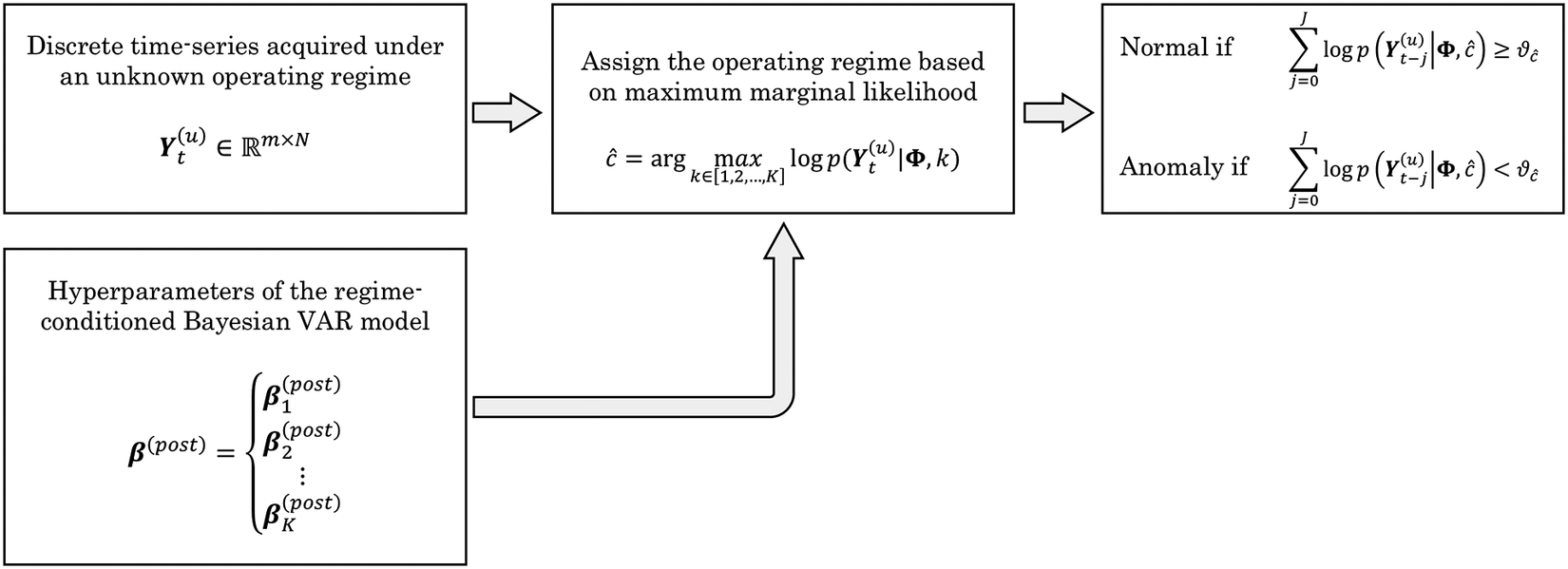
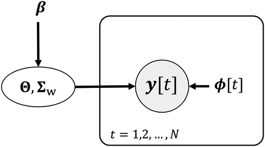
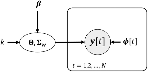

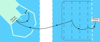
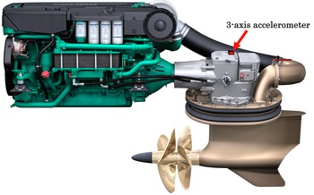
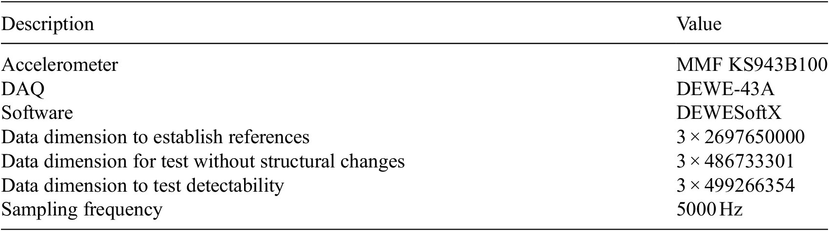
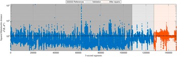
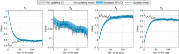
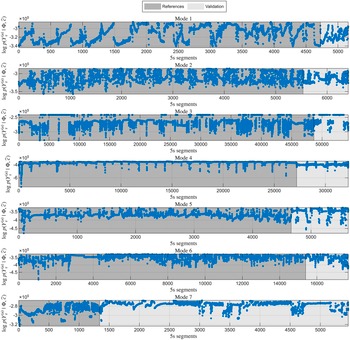

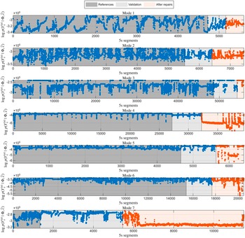
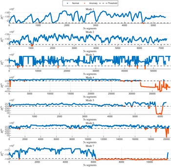

 Open access


Comments
No Comments have been published for this article.