


Introduction
Iceberg calving, i.e. the release of icebergs at the edge of marine-terminating glaciers, contributes significantly to ice sheet mass loss. Almost half of Antarctica's mass loss occurs through calving, while the other half is dominated by submarine melting of ice shelves (Depoorter and others, Reference Depoorter2013). In contrast, about 60% of Greenland's 1991–2015 mass loss was caused by surface melt and the remaining 40% by calving and submarine melt (Van den Broeke and others, Reference Van den Broeke2016). Currently, mass loss from the Greenland Ice Sheet induces a global mean sea level rise of 0.77 ± 0.07 mm a−1, which is twice as much as the contribution from the Antarctic Ice Sheet (Bamber and others, Reference Bamber, Westaway, Marzeion and Wouters2018; Imbie team, 2018). A significant part of the uncertainty of future sea-level rise projections is caused by the uncertainty in calving parametrizations (Bulthuis and others, Reference Bulthuis, Arnst, Sun and Pattyn2019).
Observations in Greenland show that for some glaciers, large-scale infrequent calving events dominate the ice mass loss over small frequent events (Walter and others, Reference Walter2010; James and others, Reference James, Murray, Selmes, Scharrer and O'Leary2014; Åström and others, Reference Åström2014; Medrzycka and others, Reference Medrzycka, Benn, Box, Copland and Balog2016; Jouvet and others, Reference Jouvet2017; Minowa and others, Reference Minowa2019). Since the physical mechanisms triggering small- and large-scale events differ (Medrzycka and others, Reference Medrzycka, Benn, Box, Copland and Balog2016), there is a need for research focused on each characteristic calving size, and in particular on large-scale events. In this context, we mean ‘large-scale’ in relation to a glacier's mass loss through calving, even if the iceberg size may be small in comparison to calving events on larger glaciers or ice shelves.
Calving mechanisms are still not entirely understood. There is a lack of data to constrain mechanical properties related to ice fracturing (Pralong and Funk, Reference Pralong and Funk2005), for instance observed critical strain rates for crevasse initiation span over two orders of magnitude (Colgan and others, Reference Colgan2016). Although there have been major advances in modelling calving in recent years (Benn and Åström, Reference Benn and Åström2018), defining a universal calving law remains a topic of research. Besides that, the complexity of calving is also due to its interconnection with other physical processes such as supra- and subglacial hydrology, or submarine melt (Benn and others, Reference Benn, Warren and Mottram2007). Melt- or seawater entering crevasses can promote crevasse growth through hydro-fracturing (Van der Veen, Reference Van der Veen2007). The water exerts a force on the side walls of the crevasse, which opposes the creep closure force of the ice and thus facilitates crevasse opening. However, our understanding of calving induced by hydro-fracturing is limited by difficulties of measuring the water level inside crevasses, especially near calving fronts for accessibility reasons. Therefore, little is known from observations about the influence of water filling of crevasses on calving.
The importance of water filling of crevasses has been addressed by numerical modelling. For a two-dimensional flowline model of Columbia Glacier, it was shown that the calving rate modelled by a crevasse-depth calving criterion highly depends on water depth in surface crevasses, a change of just a few metres in water depth changed the glacier from advancing to retreating (Cook and others, Reference Cook, Zwinger, Rutt, O'Neel and Murray2012). A two-dimensional plan-view ice-sheet model showed a similarly strong dependence of the crevasse-depth calving criterion to water depth for several Greenlandic glaciers (Choi and others, Reference Choi, Morlighem, Wood and Bondzio2018). Over the recent years, modelling individual calving events in three dimensions has become computationally affordable. A three-dimensional crevasse-depth calving model was able to reproduce observed calving behaviour without including water filling of crevasses above sea level (Todd and others, Reference Todd2018). However, such models need to be validated against high spatial and temporal resolution observations of calving events, which remain rare (Benn and others, Reference Benn, Cowton, Todd and Luckman2017b).
Submarine melt may also induce calving by undercutting grounded glacier termini (Truffer and Motyka, Reference Truffer and Motyka2016; Luckman and others, Reference Luckman2015; O'Leary and Christoffersen, Reference O'Leary and Christoffersen2013; Münchow and others, Reference Münchow, Padman and Fricker2014). Recently, a strong spatial variability in submarine melting has been observed by sonar imaging of calving fronts in West Greenland (Fried and others, Reference Fried2015; Rignot and others, Reference Rignot, Fenty, Xu, Cai and Kemp2015) and Svalbard (How and others, Reference How2019). Zones with largest undercuts are usually located in front of a plume, where meltwater is released subglacially and rises rapidly through the denser seawater. By turbulent mixing, the plume entrains relatively warm seawater such that it melts or mechanically erodes the glacier front under the waterline (Jenkins, Reference Jenkins2011; Benn and others, Reference Benn, Cowton, Todd and Luckman2017b). Modelling suggests that a so-called ‘calving multiplier effect’ exists, where long-term calving rates may be several times greater than submarine melt rates (O'Leary and Christoffersen, Reference O'Leary and Christoffersen2013; Benn and others, Reference Benn2017a; Vallot and others, Reference Vallot2018). Unfortunately, observations of undercut sizes also remain too limited to confirm a possible multiplier effect.
Here, we investigate two major and very similar calving events observed in-situ at Bowdoin Glacier, Northwest Greenland, using GPS, a terrestrial radar interferometer (TRI) and Unmanned Aerial Vehicle (UAV) flights. The two calving events were observed during two field campaigns, one in July 2015 (previously reported in Jouvet and others, Reference Jouvet2017) and one in July 2017. Satellite imagery furthermore showed similar major events since the glacier stabilized to its current calving front position in 2013 (Jouvet and others, Reference Jouvet2017; Minowa and others, Reference Minowa2019), indicating a typical calving pattern at Bowdoin Glacier. For the July 2015 event, just one record of crevasse opening is available (Jouvet and others, Reference Jouvet2017). For July 2017, TRI-derived crevasse opening rates are available every 2 h in the last 3 days prior to calving. The level of detail in the available data combined with numerical modelling provides an unique opportunity for an in-depth analysis that may reveal the physical mechanisms triggering such recurrent large-scale events. For that purpose, we use the ice flow model Elmer/Ice (Gagliardini and others, Reference Gagliardini2013) to investigate the crevasse opening leading to the 2017 calving event. Seddik and others (Reference Seddik2019) used the same model to test the sensitivity of Bowdoin Glacier's ice flow to tidal forcing, but here we focus on the opening of the single large crevasse prior to calving. Our modelling investigates the influence of several relevant processes on the crevasse opening such as tides, the presence of an undercut and surface meltwater input into the crevasse.
Study site
Bowdoin Glacier is an ~3 km wide marine-terminating glacier located in Northwest Greenland (77°N, 68°W, Fig. 1). In 2013, the glacier was up to 250 m thick at the grounded calving front. The flow velocity of ice reached a maximum of 440 m a−1 in 2013 (Sugiyama and others, Reference Sugiyama, Sakakibara, Tsutaki, Maruyama and Sawagaki2015). Satellite imagery has shown that, except for a 230 m retreat from 1999 to 2001, the terminus position was fairly stable from 1987 to 2008, when rapid retreat began (Sugiyama and others, Reference Sugiyama, Sakakibara, Tsutaki, Maruyama and Sawagaki2015). Since 2013, the calving front has stabilized to its current position, but the glacier has been thinning at a rate of 4 m a−1 (Tsutaki and others, Reference Tsutaki, Sugiyama, Sakakibara and Sawagaki2016).
Map of Bowdoin Glacier. The star in the upper left inset indicates the position of Bowdoin Glacier in Greenland (Source: MODIS). The Sentinel-2A satellite image shows Bowdoin Glacier on 25 July 2017, and is annotated with the location of the terrestrial radar interferometer (TRI) and the GPS stations (A–D). The thick black lines show the inflow boundaries of the two numerical modelling domains used in this study.
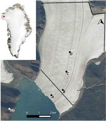
Bowdoin Glacier has been extensively studied during five summer field campaigns from 2013 to 2017. Field activities included in-situ GPS, radar measurements for bed topography and sonar for fjord bathymetry (Sugiyama and others, Reference Sugiyama, Sakakibara, Tsutaki, Maruyama and Sawagaki2015; Tsutaki and others, Reference Tsutaki, Sugiyama and Sakakibara2017), seismic monitoring (Podolskiy and others, Reference Podolskiy2016), borehole drilling and the installation of automated cameras. From 2015, unmanned aerial vehicle (UAV) flights have been operated to monitor the dynamics of ice and plumes surfacing next to the glacier front (Jouvet and others, Reference Jouvet2018). In 2016 and 2017, a terrestrial radar interferometer (TRI) was also installed on a hill opposite the calving front (Fig. 1).
Bowdoin Glacier is particularly suitable for in-situ measurements near the calving front, due to the presence of an almost crevasse-free walkable medial moraine ~1 km away from the eastern glacier margin (Fig. 1). The 25-m-wide moraine was formed by the surface transport of rocks from a confluence located ~15 km upstream the glacier front. The moraine forms a depression of the glacier surface. A stream covers part of the moraine, transporting meltwater to the glacier front.
Observations of two similar major calving events
In 2017, a crevasse across the medial moraine was already present when team members of the field campaign observed the calving front for the first time on July 3. On July 8 around 02.00 AM UTC, a 650-m-wide, 80-m-long slice calved off (Fig. 2). UAV imagery shows that the crevasse tip did not propagate horizontally until the last survey on July 7, 12 h prior to calving (Fig. S2). The height of the ice cliff above the sea level was ~30 m where the calving event took place. Time-lapse images show that the iceberg rotated backwards during the calving event (Supplementary Movie). Sentinel-2A imagery shows that the July 8 event is the first major calving event of 2017, coinciding with break-up of ice mélange. The meltwater plume was first visible through the ice mélange (Fig. 2) on the Sentinel-2A image of July 4, but not yet on the preceding image taken June 30.
UAV-derived ortho-images (a–c and e) and a Landsat 8 Operational Land Imager panchromatic image (d). Figure (a) shows Bowdoin Glacier's terminus on 5 July 2017 prior to the calving events, followed by zooms of the calved area before the calving events (b, 16 July 2015 and c, 5 July 2017) and after the events (d, 30 July 2015 and e, 14 July 2017). Figures (b–e) have the same scale (scalebar in e). Figures (a and c) also show a plume surfacing close to the moraine. The white lines (d–e) show the calving front position prior to the calving events, not corrected for glacier flow.
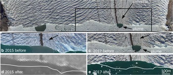
The crevasse leading to calving in July 2017 is strikingly similar to the one that appeared across the medial moraine during the summer field campaign in July 2015. Two weeks after the crevasse initiation, an ~1-km-wide and 100-m-long slice of the front collapsed (Jouvet and others, Reference Jouvet2017). Both crevasses leading to the events initiated in an area of high horizontal shear (Fig. 4), possibly caused by shallow or frozen bedrock immediately behind the front (Jouvet and others, Reference Jouvet2017). In 2015 and 2017, the crevasses responsible for major calving events were presumably filled with fresh water by a stream present on the moraine, and also possibly by seawater through a connection to the ocean. In this paper, we focus exclusively on observations and modelling of the calving event in 2017.
Observational methods
This section describes each observational method to monitor ice dynamics at the calving front used in this study, namely: UAV photogrammetrical surveys, GPS measurements, terrestrial radar interferometry, feature-tracking of satellite imagery and time-lapse imagery.
The light, fixed-wing UAV ‘SenseFly eBee’ (www.sensefly.com) was used here to conduct photogrammetrical surveys on July 5, 6, 7 and 12. Each mission consisted of two flights, covering the terminus of Bowdoin Glacier by four lines parallel to the calving front. The UAV was programmed to take aerial photographs with an overlap of 90% in flight direction and 75% in cross-flight direction. Ortho-images and digital terrain models of the calving front were processed from UAV aerial images by Structure-from-Motion photogrammetry using Agisoft PhotoScan software (www.agisoft.com, Figs 2 and S2).
Four GPS stations were installed from July 7 to 16, including one located close to the calving front (Fig. 1). These stations consisted of dual-frequency GPS receivers, which provide three-dimensional coordinates by processing the continuously recorded GPS data with a static positioning technique. Typical positioning errors were several millimetres in the horizontal direction (Sugiyama and others (Reference Sugiyama, Sakakibara, Tsutaki, Maruyama and Sawagaki2015) for details).
Velocity data were also obtained from a TRI, in this case a Gamma Portable Radar Interferometer, developed by GAMMA Remote Sensing and Consulting AG, Switzerland. The TRI was installed on a hill facing the calving front at an elevation of 496 m about 3 km away from the front (Fig. 1). Measurements were acquired in a 1-min interval from July 4 19:36 to July 12 23:06 UTC with a final resolution at the glacier front of 3.75 m in range and 5 m in azimuth. The interferograms were produced following the workflow described by Caduff and others (Reference Caduff, Schlunegger, Kos and Wiesmann2015) and were stacked over 4 h to reduce noise before phase unwrapping using features on stable terrain. The unwrapped phases were then converted to line-of-sight displacement (Werner and others, Reference Werner, Strozzi, Wiesmann and Wegmüller2008). The resulting velocity fields were resampled to the Cartesian UTM19N grid using nearest neighbour interpolation.
Third, a velocity field with a resolution of 20 m was derived from Sentinel-2A images from July 4 and 24 using IDMatch, a software package for Image and DSM Matching to derive glacier surface velocities (www.github.com/sgindraux/IDMatch). Input parameters for IDMatch are given in Supplementary Table S1. Additionally, the velocity field was filtered by a two-dimensional median filter with a 7 × 7 kernel to remove noise due to matching failure.
Finally, an automatic camera produced time-lapse imagery of the calving front (Supplementary Movie). Pictures were taken every minute from a distance of 3 km of the calving front, at the same location as the TRI (Fig. 1).
Numerical model
To analyse the drivers of crevasse opening, the terminus of Bowdoin Glacier was modelled using the finite element code Elmer/Ice (Gagliardini and others, Reference Gagliardini2013), which solves the Stokes equations in three dimensions, using Glen's law to describe the viscous behaviour of ice (Glen, Reference Glen1955). The temperature-dependent rate factor in Glen's flow law is computed using the Arrhenius relation (Paterson, Reference Paterson1994). The englacial temperature is applied according to a temperature profile measured in a borehole in 2015, and generalized as a function of depth below the ice surface over the whole domain (Jouvet and others, Reference Jouvet2017). The recorded temperature has a minimum of −10° C near the surface and is at the pressure melting point near the bed (260 m deep). The rate factor is multiplied with an enhancement factor E that can account for ice softening due to damage and ice impurities. Here we use two different set-ups, E = 1 and E = 4, with the latter value taken from Jouvet and others (Reference Jouvet2017). The enhancement factor E can be seen as a function of a damage variable d that parametrizes the density of microcracks, which affect the mechanical behaviour of ice (Pralong and Funk, Reference Pralong and Funk2005). In this formulation, the ice is considered undamaged for d = 0 (or E = 1). The enhancement factor E = 4 corresponds to a damage level of d = 0.37, i.e., 37%, according to the relation E = 1/(1 − d)n as derived in Krug and others (Reference Krug, Weiss, Gagliardini and Durand2014). Hence d = 0.37 and thus E = 4 already approaches the critical damage value d = 0.56 determined by laboratory tension tests (Mahrenholtz and Wu, Reference Mahrenholtz and Wu1992).
Model domains
Two domains were modelled: a large domain covering the lowest 7 km of the glacier terminus and a small domain restricted to the lowest 1 km (Fig. 1). The large domain serves to tune our flow parameters to match observed and modelled velocities, with limited influence of the inflow boundary condition. The small domain – coinciding with the area covered by the UAV – includes the observed crevasse and is used to explicitly model its opening rates in advance to calving.
For the large domain, surface and bedrock elevation are similar to the ones derived by Seddik and others (Reference Seddik2019) except within the last 1 km, where the bedrock DEM was updated using new sonar and ice radar data (Fig. S1) obtained during the 2016 and 2017 field campaigns. For the small domain, the updated bedrock DEM and the high-resolution surface DEM derived from the 5 July 2017 UAV flight are used. The calving front geometry is taken from the observed position on 5 July 2017. As there are no observations of the shape of the submerged part of the calving front available, the front is assumed to be a vertical cliff in most numerical experiments. For some sensitivity experiments, a submarine undercut is introduced.
Boundary conditions
The ice surface is assumed to be stress-free. At the calving front, where ice and seawater are in contact, we apply a hydrostatic pressure:

where

Here, ρ sw is the seawater density, g the gravitational constant and the sea level is denoted as z sl. The coordinate system is such that the average sea level is at z = 0 and negative z is below sea level.
We consider the effect of water pressure on the crevasse. From Figure 2, it is unclear whether the crevasse has a hydraulic connection with the sea. Other sources of water are the meltwater stream running on the moraine and possibly a connection to the meltwater that is transported to the calving front along the glacier bed, feeding the plume. Therefore, we consider two cases for the crevasse: (i) it is filled with seawater and (ii) it is filled with fresh meltwater. The boundary condition in the crevasse is equal to Eq. 1 but the water pressure

where ρ is either the density of fresh water or seawater and z wl is the water level inside the crevasse. The values of the constants used in modelling experiments are given in Table 1. As the water within the crevasse may have been a mixture of fresh and seawater, these two cases should be understood as upper and lower bounds of possible water densities.
Physical model constants used in the numerical experiments.

The bedrock is regarded as rigid and the normal basal velocity is set to zero at the ice–bed interface. At the glacier bed, we apply a linear friction law as in Gillet-Chaulet and others (Reference Gillet-Chaulet2012):

where τ b is the basal shear stress, u b the sliding velocity and C > 0 a spatially varying sliding coefficient. The satellite-derived velocity is used to inversely determine the sliding coefficient C in the large domain (Gillet-Chaulet and others, Reference Gillet-Chaulet2012). The entire glacier is assumed to be grounded (Sugiyama and others, Reference Sugiyama, Sakakibara, Tsutaki, Maruyama and Sawagaki2015). The bedrock elevation and UAV-derived surface DEM give that the height above flotation close to the front was about 10 m.
For the large domain, the observed surface velocity is applied as a Dirichlet condition on the upstream and the lateral boundaries throughout the entire depth. Because the lateral margins are thin and ice flow is little there, the application of a Dirichlet condition does not have a strong influence on our basal inversion. For the small domain, the depth-varying velocity modelled for the large domain is applied as boundary condition on the upstream and lateral boundaries.
Remeshing
For both modelled domains, the Gmsh mesher (Geuzaine and Remacle, Reference Geuzaine and Remacle2009) was used to build an unstructured three-dimensional mesh, with a characteristic horizontal edge length of 50 m and vertical mesh length of 10 m for the large domain and both horizontal and vertical edge length of 10 m for the small domain. To investigate the crevasse opening, a new three-dimensional remeshing routine was employed in Elmer/Ice that uses Mmg (Dapogny and others, Reference Dapogny, Dobrzynski and Frey2014). The remeshing routine takes the crevasse-free mesh and introduces a crevasse, which horizontal location and depth are user-specified. Here, the crevasse location is visually inferred from the UAV ortho-image of July 5 (Fig. 2). On the southeastern edge, the crevasse is open to the ocean (Fig. 7). The horizontal crevasse extent is the same for all simulations while different crevasse depths are tested (Fig. 3). Meshes are built with crevasses extending from the surface to $z=10\comma\; 0\comma\; -10\comma\; \ldots \comma\; -200$ m.
m.
Schematic overview of the physical parameters involved in the numerical experiments: the crevasse depth D below z = 0, the difference between sea level and water level in the crevasse ΔWL = z wl − z sl, the radius of the spherical undercut UC and the enhancement factor E that affects ice deformation. The supraglacial meltwater stream is also indicated.

The remeshing routine also allows us to introduce a spherical undercut at a user-specified location and radius (Fig. 3). We prescribe the undercut at the base, below the surface position of the plume observed by the UAV on July 5 (Fig. 2, z = −200 m) with various radii of $20\comma\; 40\comma\; \ldots, 120$ m, which is within the range of observed undercuts (Rignot and others, Reference Rignot, Fenty, Xu, Cai and Kemp2015).
The remeshing to account for both crevasse and undercut is done in two steps. First, the library MMG3D_mmg3dlib is called to refine the mesh where the crevasse and undercut are introduced. Second, the shortest distance to the crevasse or undercut surface is computed for each node on the refined mesh. Then, the library MMG3D_mmg3dls is used to remove the part of the mesh that is within the crevasse or within the radius of the undercut, creating a new smooth boundary surface.
Experiment design
To analyse the key drivers of crevasse opening, a series of diagnostic sensitivity experiments is conducted with varying enhancement factor E, crevasse depth D, undercut size UC and difference between sea level and water level inside the crevasse ΔWL (Fig. 3). For each set-up, Elmer/Ice was used to calculate the ice velocity, from which the crevasse opening rates are derived. These rates are compared to the TRI observations in order to find out which parameter set fits the observations best.
Results
Observed velocities
To assess measurement uncertainty, both satellite and TRI velocities are compared to in-situ GPS measurements. The differences are below 14% for satellite-derived and 12% TRI-derived velocities, as described in more detail in the Supplementary Material (Fig. S3). Vertical displacement derived from GPS measurements does not show a clear tidal signal (not shown), which also indicates the glacier is grounded.
Figure 4a shows the mean velocity field obtained for the 4–24 July period inferred from the satellite images. The velocity field shows a strong gradient, with lower velocities in the east where the glacier has a shallow bed (Sugiyama and others, Reference Sugiyama, Sakakibara, Tsutaki, Maruyama and Sawagaki2015; Jouvet and others, Reference Jouvet2017). The highest gradients indicate a shear-zone, which starts close to the location where the moraine reaches the glacier front (Fig. 4a) and a shallow bedrock underlies the slow flowing region (Fig. S1). The shear-zone deviates from the moraine further upstream, turning towards the eastern glacier margin around 8625 km Northing (Fig. S1).
Satellite-derived velocity field during 4–24 July period (a) and TRI-derived velocity field in line of sight of the TRI averaged between July 4 19:51 and July 12 22:51 UTC (b). The background of both panels consists of the July 4 Sentinel-2A image and the white line indicates the zone of highest shear. The coordinate projection is a Cartesian UTM19N grid.
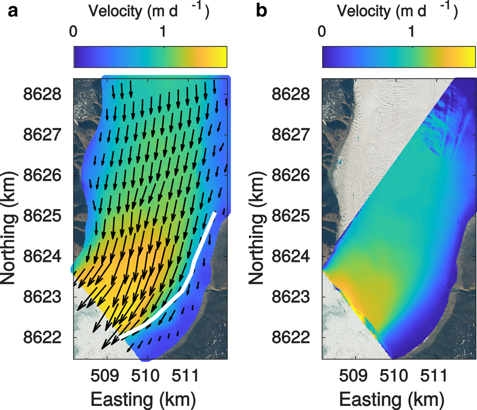
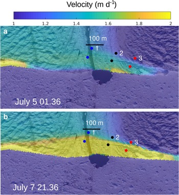
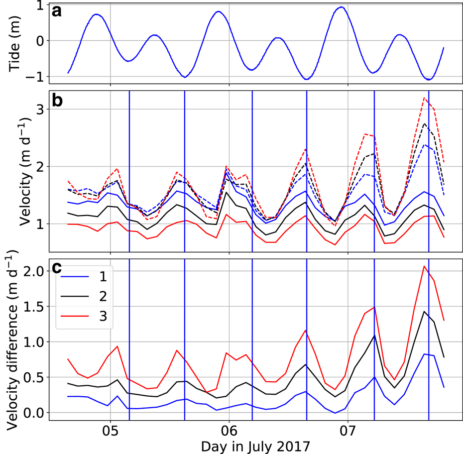
The spatial distribution of the velocity measured by the TRI averaged over the entire measurement period is given in Figure 4b. The whole front of Bowdoin Glacier is captured, but a hill on the western glacier margin masks part of the glacier further upstream. Figure 5 shows 2 h average velocity distributions near the crevasse, shortly after the TRI started operating (July 5, 00:36-02:36 UTC) and shortly before the calving event (July 7, 20:36-22:36 UTC). The opening of the crevasse is clearly visible by a discontinuity in the observed velocity field. Three points on each side of the crevasse were chosen, for which the velocity time series inferred by TRI was extracted. These points were selected immediately upstream and downstream of the crevasse in line of sight of the TRI to determine the crevasse opening rates. As the crevasse is not exactly perpendicular to the line of sight of the TRI, the latter does not capture the entire motion and underestimates the opening rates. The temporal evolution of the velocity at the points on each side of the crevasse are shown in Figure 6, together with the velocity difference (i.e. opening rates) and the tide. Velocity is highest at, or slightly before, low tide. Opening rates vary along the crevasse and with time from 0.03 to 0.79 m d−1. Also the opening rate is highest at, or slightly before, low tide. Hence, the tidal influence on the ice flow is twofold: besides the velocity also the longitudinal stretching of the glacial surface increases at low tide, which was also noted by Podolskiy and others (Reference Podolskiy2016). While the tidal variations of the opening rates are of similar amplitude during the first 36 recorded hours, the opening rates increase irreversibly within the next 36 h preceding the calving event (Fig. 6).
TRI-derived 2 h average velocity field in line of sight of the TRI on (a) July 5 00:36-02:36 and (b) July 7 20:36-22:36 UTC, overlayed on the UAV ortho-image taken on July 5. Three points on each side of the crevasse are chosen, for which the velocity time series are extracted in Figure 6.
Tidal height (a) as measured at Thule Air Base, 125 km south of Bowdoin Glacier, provided as a part of the Global Sea Level Observing System network (www.gloss-sealevel.org). Velocity time series in line of sight of the TRI (b) for each chosen point upstream (continuous line) and downstream (dashed line) the crevasse. Each point is colour coded consistently with Figure 5. Velocity difference of the points across the crevasse is shown in (c). The vertical blue lines show when low tide occurred.
Sensitivity experiments
Inversions for basal drag coefficient are carried out on the large domain (Fig. 1), to reproduce the averaged velocity inferred from satellite images (Fig. 4). The inversion is done for both E = 1 and E = 4. The resulting velocity, sliding coefficient and misfits are given in the Supplementary Material (Figs S5 and S6). The two basal sliding inversions are used as a starting point to investigate the opening of the crevasse in the small model domain.
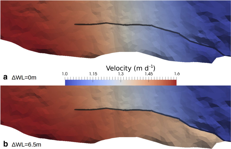
We ran several numerical experiments changing the water level in the crevasse from ΔWL = 0 to ΔWL = 6.5 m, while keeping the sea level at 0 m, and assuming the crevasse is filled with fresh water. The largest tested water-level difference ΔWL = 6.5 m is the one for which the fresh water pressure and sea water pressure are equal at the deepest point of the bed underneath the crevasse (z = −240 m), which forms an upper bound for ΔWL in case a hydraulic connection with the sea imposes the basal pressure. The modelled velocity for a crevasse reaching to z = −100 m is shown in Figure 7 for the most extreme water levels (ΔWL = 0 and 6.5 m). The crevasse opens when ΔWL = 6.5 m, but closes when ΔWL = 0 m. To quantitatively compare the model results to observations, the modelled velocity was extracted on each side of the crevasse at points 1–3 (Fig. 5) for various crevasse depth D, water-level difference ΔWL and enhancement factor E. The modelled opening rate in line of sight of the TRI is shown in Figures 8a–c. Figures 8b and c show that for all ΔWL < 4 m, the modelled opening rate is below all observations at points 2 and 3 for any crevasse depth. Only the most extreme water level (ΔWL = 6.5 m) and a crevasse depth of D = 100 m (for E = 4) or D = 150 m (for E = 1) is sufficient to obtain an opening rate similar to the mean observed opening rate with the TRI. When assuming fresh water in the crevasse, the maximum observed opening rate is only reached by a deep crevasse (D = 200 m), high water level (ΔWL = 6.5 m) and very soft ice (E = 4).
Modelled velocity (m d−1) using parameters E = 1, D = 100 m for ΔWL = 0 m (a) and ΔWL = 6.5 m (b).
Opening rates over crevasse depth below z = 0 (D) (along the x-axis) for varying water-level difference, in line of sight of the TRI at the three chosen points (Fig. 5) assuming fresh water (a–c) and seawater (d–f) in the crevasse. The solid and dashed lines show the results obtained with E = 4 and E = 1, respectively. The grey area indicates the observed range of opening rates and the grey dashed line is the time averaged opening rate. Note that the scale of the y-axis is different in every panel. All simulations assume z sl = 0 m.
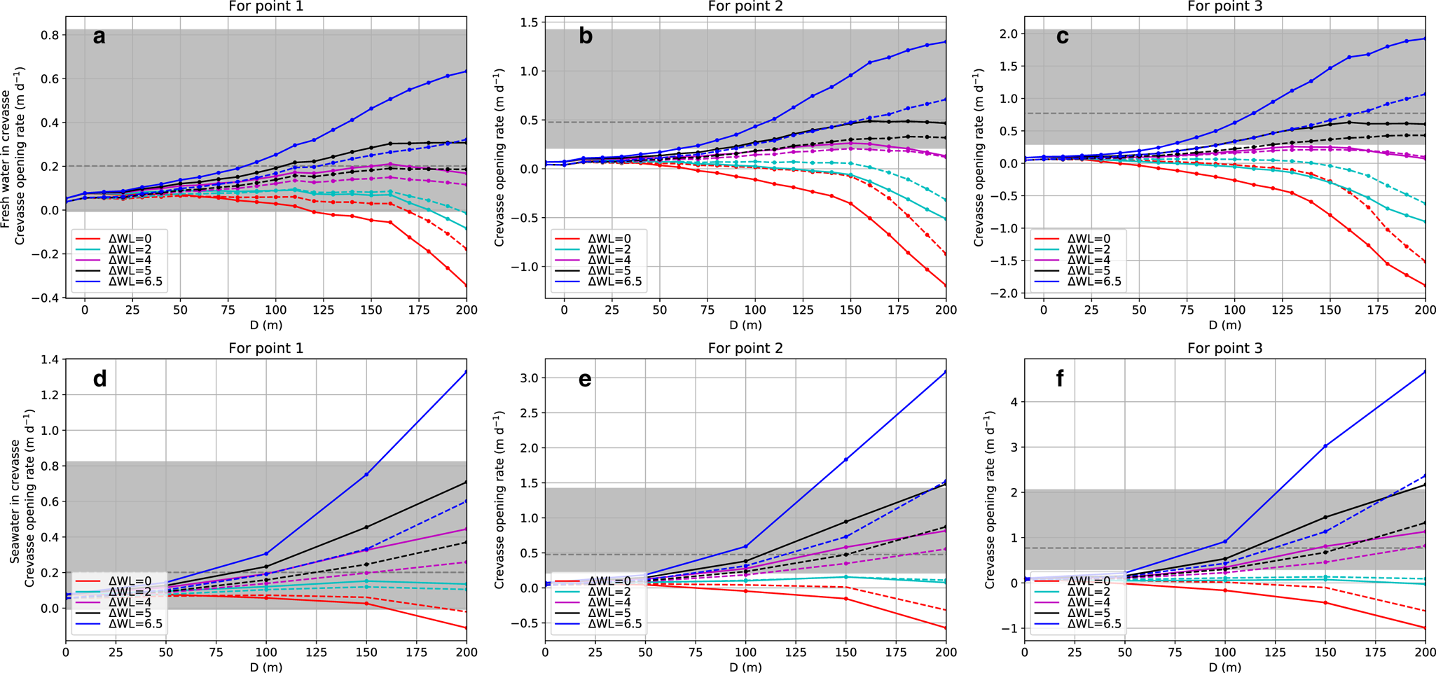
Even if the crevasse is filled with seawater, water-level difference of at least 4 m is necessary to reach the mean observed opening rate (Figs 8d–f) while all modelled opening rates are below the minimum observed value for ΔWL ≤ 2 m. Qualitatively, the opening rates for fresh water (Figs 8a–c) and seawater (Figs 8d–f) are very similar. The distribution of the modelled opening rates compared to the observed range are similar for all three points. Therefore, we only show modelled opening rates for point 3 from now on.
Additional model results show that opening rates for ΔWL = 5 m hardly vary for varying z sl = −2, 0, 2 m (Supplementary Material, Fig. S7). Changing ΔWL has a much larger impact on the opening rate than variations in sea level (Fig. S7). Therefore, we kept the sea level constant (z sl = 0 m) in all further experiments.
The influence of an undercut on the crevasse opening rate was also tested. The resulting opening rates at point 3 for D = 50, 100 and 150 m and varying ΔWL and undercut radius UC are shown in Figure 9 for a fresh water-filled crevasse. A crevasse deeper than 150 m was not modelled as the undercut then intersects the crevasse, which contradicts the assumption of a fresh water-filled crevasse. The observed opening rates for all UC and D = 50 m are much smaller than observed ones (Fig. 9a). Figures 9b and c show that the opening rate increases with the size of the undercut, but only for crevasse water levels that are sufficient to oppose viscous creep closure of the crevasse (ΔWL ≥ 4 m) and when having a large undercut of at least 60 m. If ΔWL = 0 m, the crevasse closes without undercut, but the crevasse closes even faster for a 120 m undercut in case of D = 150 m (Fig. 9c). To obtain the maximum observed opening rates for D = 150 m and ΔWL = 6.5 m, a large undercut of 80 m (for E = 4) or 120 m (E = 1) is found necessary. For D = 150 m and ΔWL = 5 m, only in the case of an undercut of 120 m and soft ice (E = 4), the modelled opening rate becomes close to the observed maximum.
Opening rates over undercut size (UC, along the x-axis) for varying water-level difference, in line of sight of the TRI at point 3 (Fig. 5) assuming fresh water (a–c) and seawater (d–f) in the crevasse. The solid and dashed lines show the results obtained with E = 4 and E = 1, respectively. The grey area indicates the observed range and the grey dashed line is the time averaged opening rate. Note that the scale of the y-axis is different and the grey area has the same magnitude for all panels.

In case the crevasse is filled with seawater, similar opening rates occur for smaller water-level differences (Figs 9d–f ). For a deep crevasse, D = 200 m, either ΔWL = 5 m and UC = 100 m are necessary for stiff ice (E = 1) or ΔWL = 4 m and UC = 80 m for softer ice (E = 4), in order to obtain the maximum observed opening rate (Supplementary Material, Fig. S8).
Reconstruction of water-level difference
In the final 36 h before calving, the opening rate was observed to accelerate from below 1 m d−1 up to 2.1 m d−1 at low tide. Our modelling results show that the acceleration of the opening rate may have been caused by increased water input, deepening of the crevasse, softening of the ice due to tidally induced cyclic fatigue, growth of an undercut or a combination of these processes. Using linear interpolation of the ensemble of simulations, we can reconstruct water-level difference ΔWL which is necessary to reproduce the observed opening rate time series. In the reconstructions, all parameters except ΔWL are kept constant in the first 36 h and E, D or UC increase linearly in the final 36 h. Sea level is kept at z = 0 and ΔWL is changed by varying the crevasse water level z wl. In order to visualize the relative importance of these drivers, we compare these scenarios to three control cases where all parameters except ΔWL are kept constant during the entire period. Figure 10 shows the reconstructed ΔWL time series for a seawater-filled crevasse for three configurations:
1. a crevasse deepening from D = 150 to 200 m, which is all the way to the bed for most of the crevasse, while keeping E = 4 constant. This scenario can explain the observed acceleration in crevasse opening, and the semi-diurnal variation of ΔWL stays on the order of the tidal amplitude, but a slight increase in ΔWL was needed over the last 36 h to reproduce observed opening rates. Additional simulations with a crevasse deepening all the way to the bed (z = −240 m) did not reduce the required ΔWL significantly.
2. an increase from E = 1 to 4, while keeping D = 200 m constant. This scenario is also capable of explaining the accelerated opening, but again a slight increase in ΔWL was needed to reproduce the observed acceleration. The difference with the crevasse deepening scenario is almost indistinguishable for a seawater-filled crevasse. For a fresh water-filled crevasse (Supplementary Material, Fig. S9), this scenario differs from the crevasse deepening case and a larger ΔWL is required in the first 36 h when E = 1 compared to the crevasse deepening case (which assumes E = 4). Further softening beyond E = 4 may reproduce the acceleration without increased ΔWL but this has not been tested.
3. an undercut growth from 100 to 110 m, which is most capable to explain the increased opening rate of all tested scenarios without requiring a further increase of ΔWL. It is sufficient to have a 1 m amplitude tidal variation around a mean ΔWL = 3 m.
Required water-level difference ΔWL in order to reproduce observed opening rates for six scenarios assuming the crevasse to be filled with seawater. The vertical blue lines show the occurrence of low tide. Dashed lines show configurations where not only ΔWL changes but also E, D or UC changes after 36 h. Note that some configurations require similar ΔWL, hence lines partially overlap (e.g., red and blue).
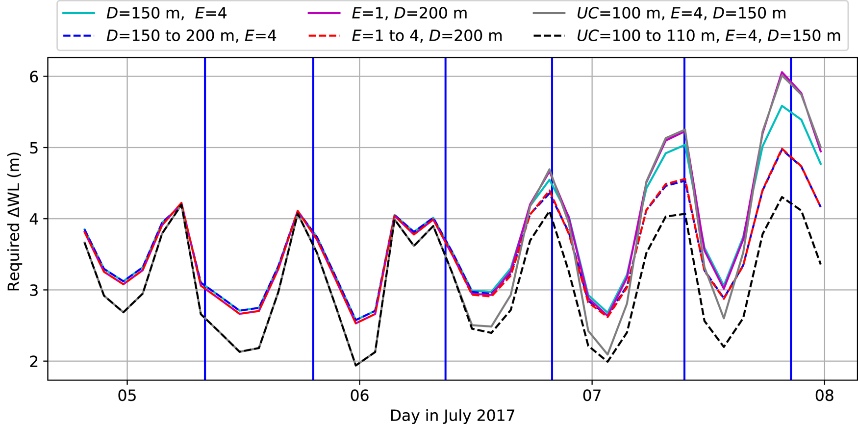
The three control cases where only ΔWL varies show that an increased water input to raise the water level by 1.5–2 m on top of the tidal variation is also sufficient to explain the acceleration (depending on the scenario, see Fig. 10).
Discussion
Importance of the water-level difference
The discontinuity of the velocity across the crevasse suggests that the crevasse reached the calving front on the south-eastern side (Fig. 5). Therefore, there may have been a hydraulic connection between the crevasse and the sea. However, there are no direct observations of the water level inside the crevasse. Our model results show a strong influence of a water-level difference between the sea and the crevasse on the opening rate (Figs 8 and 9). We find that a water-level difference of at least 4 m between the crevasse and the sea is necessary to reproduce the maximum observed crevasse opening rate at low tide shortly before calving, assuming the crevasse is filled with seawater. This suggests an inefficient hydraulic connection between the crevasse and the sea inducing a delay in water drainage from the crevasse to the sea. Presumably, the water level in the crevasse must have been above sea level at low tide. However, the tidal amplitude is only 2 m (Fig. 6). Therefore, our model results show that such a water-level difference is not sufficient to explain the observed opening rates, even when all other parameters favour crevasse opening (deep crevasse filled with seawater, large undercut and soft ice). Based on our model results, we can only explain the observed opening rates by meltwater supply of the stream that filled the crevasse exceeding sea level by at least 3 m and an inefficient hydraulic connection with the sea maintaining this water-level difference in addition to the 1 m amplitude tidal variation.
Tidal modulation of the crevasse opening rate
It has previously been shown that ice flow velocity is tide-modulated at Bowdoin Glacier, the highest speed being reached at low tide (Sugiyama and others, Reference Sugiyama, Sakakibara, Tsutaki, Maruyama and Sawagaki2015). This indicates that changes in the back pressure exerted by water along the glacier front are a first-order control in the tidal modulation of the ice flow velocity. Furthermore, Podolskiy and others (Reference Podolskiy2016) showed that microseismicity increases with low tide, driven by variations in longitudinal stretching which favours near-surface tensile crevasse openings. Our data show that the opening rate of a single, deep, crevasse is also modulated by tide. The opening is up to twice as fast at low tide compared to high tide during the first 36 h of observation (Fig. 6) and this increases to up to four times as fast during the final 36 h before collapse. As we found a strong influence of the water-level difference, the tidal modulation of the opening rate can directly be explained by the highest water-level difference at low tide (Fig. 10).
We also found that with a higher enhancement factor (E = 4), hence softer, more damaged ice, the modelled opening rate increases considerably. Therefore, cyclic fatigue of ice caused by the tidal modulation of the opening rate may explain the increasing opening rates observed in the last 36 h before the calving event. Modelling by Hulbe and others (Reference Hulbe2016) suggested that the cyclic fatigue associated with tidal flexure can indeed soften the ice. However, that study focused on floating ice shelves that accelerate at high tide and a tide-induced fatigue for a grounded glacier as Bowdoin remains to be investigated.
Plausible calving mechanisms
The calving events monitored in July 2015 and 2017 occurred at approximately the same location. For both events, the crevasses leading calving crossed the moraine (Fig. 2). This is unusual, since the moraine appears to act as a suture zone (Hulbe and others, Reference Hulbe, LeDoux and Cruikshank2010), where most crack-tips arrest (Fig. 2). We found that the calving events were controlled by persistent characteristics, which are specific to Bowdoin Glacier: (i) the asymmetrical basal topography induces a high shear zone where large crevasses initiate, (ii) a plume undercuts and destabilizes the calving front and (iii) a stream on the moraine fills crevasses that cross the moraine with water and deepens the crevasses by hydro-fracturing. As the front of Bowdoin Glacier has been stable since 2013 and these characteristics have been observed for several years (Sugiyama and others, Reference Sugiyama, Sakakibara, Tsutaki, Maruyama and Sawagaki2015), it is likely that they will persist in the future, such that similar large-scale calving events may reoccur as long as the calving front remains at its present position.
We obtained detailed temporal and spatial observations of the crevasse opening prior to the calving event in July 2017 and found that the crevasse opening accelerates during the last 36 h (Fig. 6). Figure 10 shows that a 1.5–2 m increase in water level, in addition to the tidal variation and the ~ 4 m crevasse water level above low-tide sea level, may on its own explain the large acceleration of opening rate observed. An undercut growth of 10 m is most capable of explaining the accelerated opening without requiring a further increase of water level. The submarine melting rates induced by the plume were presumably in the range of previously estimated melt rates for glaciers in Greenland (e.g., up to 8 m d−1, Xu and others (Reference Xu, Rignot, Fenty, Menemenlis and Flexas2013); Rignot and others (Reference Rignot, Fenty, Xu, Cai and Kemp2015)). Therefore, at the high end of these numbers, an undercut growth of 10 m within 36 h is plausible. Crevasse deepening and ice softening can also cause the crevasse opening to accelerate but still require an increase of water level on the order of 0.5 m to explain the acceleration. Hence, modelling demonstrates the relative importance of the drivers, but more in-situ measurements are necessary to determine which condition prevailed. For example, detailed surface melt observations or projections could be used as input data for a glacier hydrology model to constrain the water level in the crevasse using a linear reservoir model (Hock and Jansson, Reference Hock and Jansson2005). Alternatively, fjord observations could drive a plume model to provide submarine undercutting rates. Once time series of crevasse water input and submarine melting are available, a prognostic ice dynamics model could resolve which driver dominated crevasse opening. Moreover, for glacier calving fronts that are as accessible as Bowdoins front, pressure sensors deployed within a crevasse could monitor the water-level change over time which was found to be a crucial variable in this study.
Model limitations and potential improvements
Using a diagnostic numerical model, we investigated the relative importance of several physical processes responsible for the crevasse opening. Our approach has two major limitations: (i) it considers ice as a viscous material and neglects elastic deformation that occurs at short timescales and (ii) it does not account for the change of the crevasse geometry with time, nor the damage of the ice in response to load cycles.
The lower limit of the viscous relaxation timescale (the Maxwell timescale) is determined by the ratio of Glen's shear stress-dependent viscosity of ice (η) and Young's modulus (Y) (Benn and others, Reference Benn2017a). Typical values of these variables for ice indicate that η/Y ranges from less than an hour up to 12 days, which means that ice behaves as a viscoelastic medium over tidal cycles (Jellinek and Brill, Reference Jellinek and Brill1956; Reeh and others, Reference Reeh, Christensen, Mayer and Olesen2003). Since the observed major calving events lasted for at least 5 days from the first crevasse appearance to the final collapse, also for crevasse propagation both viscous and elastic deformation could have played a role. Seddik and others (Reference Seddik2019) also used Elmer/Ice to model the ice flow of Bowdoin Glacier, and investigated the sensitivity of the glacier flow to tidal forcing at the calving front. Their model underpredicted the amplitude of the semi-diurnal variability by approximately a factor three. The authors rule out that (visco)elastic material behaviour played a significant role in explaining the observed tidal-modulated flow variability because low tide and highest flow occur almost synchronously. They argue that a significant elastic response would have caused a time lag. Instead, they relate the mismatch between observed and modelled tidally-driven ice flow variability to either inaccuracies in the surface and bedrock topographies or neglected mechanical weakening due to crevassing. Although we use updated DEMs for both surface and bedrock topographies, the tidal modulation of the ice flow is still underpredicted as in Seddik and others (Reference Seddik2019) in our viscous model set-up (results not shown). However, seawater-level variations in the range of local tidal amplitude (1 m) do reproduce the observed tidal modulation of the opening rate (Fig. 10). Hence, we conclude that our model set-up is suitable to investigate the relative importance of drivers of crevasse opening, despite the assumed material property of ice (viscous). Although our set-up reproduces the timing of opening rate variations and tidal phase qualitatively, the crevasse opening may partly have resulted from elastic deformation and hence our viscous model may underestimate opening rates and thus overestimate required water levels to reproduce observations. Therefore, future modelling work of this kind should employ a viscoelastic rheology for ice, as done by Christmann and others (Reference Christmann, Plate, Müller and Humbert2016).
To account for change of geometry during the crevasse propagation, a dynamic model is required such as the one implemented by Yu and others (Reference Yu, Rignot, Morlighem and Seroussi2017), which considers viscous deformation of fractures by adapting the mesh to the fracture depth, while fracture propagation is modelled by Linear Elastic Fracture Mechanics (LEFM). However, Yu and others (Reference Yu, Rignot, Morlighem and Seroussi2017) used a two-dimensional flowline model and LEFM crevasse propagation is complex to generalize in three dimensions. An elastic discrete element model like HiDEM (Åström and others, Reference Åström2014) may be more suitable to model fracture propagation, coupled with longer term viscous deformation using the remeshing routine employed here. To model only damage increase but not fracture propagation, it would be sufficient to use a similar model set-up as Krug and others (Reference Krug, Weiss, Gagliardini and Durand2014), which implements damage initiation or growth based on a tensile stress criterion.
Conclusions
This study focused on the calving behaviour of Bowdoin Glacier, Northwest Greenland. Two major calving events from summers 2015 and 2017 were investigated, based on a comprehensive observational data set and a numerical flow model. The ice mass lost during such events contributes significantly to the yearly calving mass loss, suggesting that our detailed observations are key to understanding the general calving behaviour at Bowdoin Glacier. Our terrestrial radar interferometry data revealed a tidal modulation of the opening rate of a crevasse which ultimately led to calving. The opening rate is doubled at low tide and accelerated during the last 36 h prior to calving at which point there was a factor four difference in opening rate between high and low tide.
Experiments with the three-dimensional full-Stokes ice flow model Elmer/Ice showed that the modelled opening rate is highly sensitive to crevasse water level. In addition, a variation of sea water level in the range of the tidal amplitude (1 m) explains the observed semi-diurnal variations in opening rate. Furthermore, modelling results revealed that the accelerated opening rates prior to calving can be explained by increased meltwater input, crevasse deepening, damage increase or undercutting of the glacier front. More observations to drive a dynamic model including submarine melt rates and meltwater input to the crevasse would help to determine which of these processes is primarily responsible for crevasse growth and calving. Our data and modelling results show the importance of tides and hydro-fracturing by surface meltwater input to control the opening of crevasses prior to major calving events at Bowdoin Glacier. These mechanisms should be included in more general parametrizations of iceberg calving.
Supplementary material
To view supplementary material for this article, please visit https://doi.org/10.1017/jog.2019.89.
Contribution statement
EvD and GJ designed the study. EvD implemented the remeshing routine and carried out the numerical simulations with support from JT, TZ and GJ. AW performed the collecting and processing of the TRI data and operated the UAV in 2017. MF and SS organized the fieldwork at Bowdoin Glacier. SS and IA provided GPS and bed elevation data. EvD drafted the manuscript with support from GJ and all authors contributed to the final version.
Data
Data is available on request.
Acknowledgments
We thank the members of the 2015 and 2017 field campaigns on Bowdoin Glacier. We acknowledge Julien Seguinot for providing tidal data, Sentinel-2A satellite images processed with Sentinelflow (https://doi.org/10.5281/zenodo.1774659) and for valuable feedback on the abstract. We also thank Saskia Gindraux for deriving the velocity field from Sentinel2A images with IDMatch and Fabian Neyer for support with UAV photogrammetry. This research is part of the Sun2ice project (ETH Grant ETH-12 16-2), supported by the Dr. Alfred and Flora Spälti and the ETH Zurich Foundation. Field work was funded by the Swiss National Science Foundation, grant 200021-153179/1, and the Japanese Ministry of Education, Culture, Sports, Science and Technology through the Arctic Challenge for Sustainability (ArCS) project. Implementation of the remeshing routine has been performed under the Project HPC-EUROPA3 (INFRAIA-2016-1-730897), with the support of the EC Research Innovation Action under the H2020 Programme; in particular, we gratefully acknowledge the support of Peter Råback and the computer resources and technical support provided by CSC in Finland. We thank the editor Frank Pattyn and the referees for their constructive comments, which contributed to improve the manuscript.


 Open access