1 Introduction
Cold-climate coastlines, found in Arctic, Baltic and Antarctic sea regions, are characterized by the seasonal presence of sea ice, which significantly influences coastal dynamics, offshore structures, and marine navigation [Reference Meylan, Bennetts, Cavaliere, Alberello and Toffoli26, Reference Meylan and Squire28]. Understanding wave–ice interactions in such environments is crucial for predicting ice loads, evaluating coastal resilience, and designing safe and efficient engineering structures. In polar oceans, sea ice appears either as broad, continuous sheets or as collections of smaller, rounded pancake floes that drift on the water surface. As ocean waves travel through these ice-covered zones, their energy gradually diminishes due to scattering by the ice floes and various dissipative mechanisms within the ice–water system. Sea ice acts as an elastic layer at the water surface. Modifying wave propagation has been studied for some time. Numerous works, such as Squire [Reference Squire43], Montiel and Squire [Reference Montiel and Squire30], have highlighted the importance of modelling sea ice as an elastic or viscoelastic plate to capture its realistic dynamic behaviour. Recently, there has been growing interest in the role of ice in energy dissipation, which is crucial for engineering applications in Arctic and sub-Arctic regions. Experimental and numerical studies by Zhao and Shen [Reference Zhao and Shen49], Herman et al. [Reference Herman, Cheng and Shen16], and others have demonstrated this. Another important aspect is the presence of compressive forces in the ice, which may give rise to tension or compression depending on weather conditions. The effects of these forces on wave interaction and propagation have been examined by Mohanty and Sidharth [Reference Mohanty and Sidharth29], Malenko and Yaroshenko [Reference Malenko and Yaroshenko22], among others. These effects are not considered in the present analysis and may serve as a promising direction for future research.
The theoretical foundation for describing the mechanical behaviour of ice-covered ocean was laid by Greenhill [Reference Greenhill12] who represented the ice sheet as an elastic beam. Building on this, Fox and Squire [Reference Fox and Squire11] employed a computational mode-matching technique to examine the reflection and transmission of oblique water waves at the boundary of shore-fast sea ice. Squire [Reference Squire41, Reference Squire42] highlighted the wave–ice interaction phenomenon and found that the outcomes are connected to the study of wave interaction with very large floating structures. In the context of two-dimensional linearized hydroelasticity, Sturova [Reference Sturova45] analysed small oscillations of a submerged body partially covered with ice. Additionally, in a separate study Sturova [Reference Sturova44] introduced a new theoretical framework for analysing unsteady three-dimensional sources in deep water under an elastic ice plate. Previous research has shown that ice can significantly affect coastal environments, contributing to shoreline erosion and impacting marine life. However, the presence of submerged structures such as coastal barriers and breakwaters adds further complexity to the interaction process. The deployment of vertical barriers is one approach for mitigating beach erosion. The present study assumes that the ocean surface, covered by a thin sheet of floating ice, is modelled as a thin elastic plate, while the barriers are represented as submerged porous elastic plates.
The interaction of waves with submerged structures has been studied for a long time. Dean [Reference Dean8] investigated the behaviour of normally incident waves encountering a fully submerged vertical barrier that extends upward from a point below the water surface. Using complex variable methods, he provided an exact analytical solution to this classic wave–structure interaction problem. Numerous studies on vertical rigid barriers can be found in the works of various authors (see, for example, [Reference Evans10, Reference Morris31, Reference Newman32, Reference Porter34, Reference Ursell46]). In recent times, Ding et al. [Reference Ding, Yue, Sheng, Wu and Zou9] explored the phenomenon of Bragg reflection caused by multiple vertical thin plates. To prevent heavy wave action porous breakwaters offer a cost-effective and environmental friendly alternative to traditional designs, as they help support aquaculture and reduce water pollution. The foundation for studying wave interaction with porous structures was laid by Sollitt and Cross [Reference Sollitt and Cross40], who applied Darcy’s law to model wave scattering by porous barriers. Their work has since influenced a wide range of subsequent studies. Chwang [Reference Chwang7] introduced a porous wavemaker theory to investigate the generation of small-amplitude surface waves in finite-depth water by a horizontally oscillating porous vertical plate. Manam and Karmakar [Reference Manam and Sivanesan23] explored the relationship between wave potentials associated with porous and rigid barriers, providing a theoretical basis for comparing their hydrodynamic behaviours. Sarkar et al. [Reference Sarkar, Roy and De37] analysed the effectiveness of multiple vertical porous barriers in attenuating wave energy in a fluid domain of uniform finite depth, utilizing a multi-term Galerkin approximation approach. Gupta and Gayen [Reference Gupta and Gayen13, Reference Gupta and Gayen14] addressed the scattering of waves by two porous barriers and porous plates considering nonuniform porosity.
Moreover, flexible barriers represent another type of coastal protection structure, where flexibility aids in wave energy dissipation and also promotes cost-effective construction. Researchers including Abul-Azm [Reference Abul-Azm1], Lee and Chen [Reference Lee and Chen18] and Meylan [Reference Meylan25] have contributed to the study of flexible barriers. Combining porosity and flexibility in submerged structures has proven more effective in providing coastal protection and mitigating resonance within harbour regions. Wang and Ren [Reference Wang and Ren47] investigated the performance of flexible porous breakwaters by analysing a bottom-mounted barrier and examining the influence of different wave characteristics. Karmakar and Soares [Reference Karmakar and Soares17] studied the scattering of obliquely incident waves by multiple bottom-standing flexible porous barriers using the least-squares approximation method. Meylan et al. [Reference Meylan, Bennetts and Peter27] examined the wave scattering by circular floating porous elastic plates using the eigenfunction expansion method. Gupta et al. [Reference Gupta, Naskar and Gayen15] addressed the interaction of water waves with dual asymmetric vertical flexible porous plates by employing the hypersingular integral equation method. In another study, Singh and Kaligatla [Reference Singh and Kaligatla39] utilized the eigenfunction expansion method to examine the scattering of water waves by vertical flexible-porous barriers, emphasizing the role of structural flexibility in enhancing Bragg resonance over rippled seabeds. The scattering of gravity waves by an array floating flexible plates was considered by Boral et al. [Reference Boral, Barman and Sahoo2] in the context of wave blocking. More recently, Sasmal and De [Reference Sasmal and De38] explored the interaction of surface gravity waves with multiple flexible partially immersed porous barriers in deep water using a single-term Galerkin approach. Their findings revealed that the flexibility of porous structures plays a crucial role in diminishing wave forces on the barriers.
Despite their potential for shoreline protection, in ice-covered waters it is essential to balance structural performance with material efficiency. Considering the ice sheet as a thin elastic layer of infinite extent, several aspects of flexural gravity wave interactions with barriers and breakwaters have been analysed. Maiti and Mandal [Reference Maiti and Mandal21] investigated the influence of an ice cover on the scattering of water waves by a thin, inclined, rigid barrier submerged in infinitely deep water. Various aspects of wave scattering by two thin submerged porous plates were analysed by Chanda and Bora [Reference Chanda and Bora5, Reference Chanda and Bora6] in an ice-covered ocean and over an elastic bottom. Sarkar et al. [Reference Sarkar, Paul and De36] investigated the interaction of oblique water waves with multiple porous bottom-standing barriers in the presence of an ice-covered ocean. Within the framework of Bragg resonance and blocking dynamics, Chanda et al. [Reference Chanda, Barman, Sahoo and Meylan4] examined the interaction of flexural gravity waves with an array of bottom-standing porous barriers of nonuniform height.
The previous studies have primarily investigated flexural gravity wave interactions with submerged thin barriers. To the best of the authors’ knowledge, no such investigation has been reported in the existing literature on the scattering of flexural gravity waves by multiple submerged flexible porous plates, using an integral equation approach combined with the multi-term Galerkin technique. This has motivated the present study to fill this research gap by assessing the effectiveness of such configurations in mitigating wave impact on ice-covered coasts. Submerged structures provide several advantages, including effective storm protection, lower construction costs, suitability for poor soil foundations, minimal disruption to coastal water environments, support for natural water and sediment transport, reduced ecological impact, and minimal visual intrusion. Unlike rigid barriers, vertical flexible porous plates dissipate wave energy through both porosity and flexibility, enhancing their ability to withstand wave forces while reducing the risk of structural damage or collapse. Thus, analysing such structures can broaden the scope of effective coastal protection strategies by minimizing erosion and wave energy. Accordingly, we present a hydroelastic analysis of wave interactions with multiple submerged, thin flexible porous plates of varying lengths in a finite-depth, ice-covered ocean.
Using small-amplitude theory, the problem is reduced to a boundary value problem (BVP) along with the relevant boundary conditions in Section 2. Mode-coupling relations are then used in Section 3 to transform this BVP into a set of Fredholm integral equations, revealing a square-root singularity in the fluid velocity near the plate edges. Section 4 outlines the multi-term Galerkin method with appropriate basis functions to capture this singularity. The wave force on the porous flexible plates is derived in Section 5. Section 6 analyses the influence of key parameters on hydrodynamic responses and validates the model through comparisons with existing results. Conclusions are summarized in Section 7.
2 Mathematical model
Let an array of N thin flexible porous plates, with nonuniform lengths, be immersed in an incompressible, inviscid, and homogeneous fluid of density $\rho _w$
beneath an ice-covered ocean of finite depth H. A Cartesian coordinate system
$\rho _w$
beneath an ice-covered ocean of finite depth H. A Cartesian coordinate system $(x,y)$
is adopted with x-axis along the undisturbed ice-covered surface, and y-axis pointing downward. The fluid rests upon a rigid bed at
$(x,y)$
is adopted with x-axis along the undisturbed ice-covered surface, and y-axis pointing downward. The fluid rests upon a rigid bed at $y=H$
and expands the region
$y=H$
and expands the region $-\infty <x<\infty $
in the horizontal direction. The flow is assumed to be irrotational and time-harmonic with angular frequency
$-\infty <x<\infty $
in the horizontal direction. The flow is assumed to be irrotational and time-harmonic with angular frequency $\omega $
. The N porous elastic plates with jth plate at
$\omega $
. The N porous elastic plates with jth plate at $(a_j,b_j)$
, partition the domain into
$(a_j,b_j)$
, partition the domain into $N+1$
sub-regions
$N+1$
sub-regions $S_j~(j=1,2, \ldots , N+1)$
, as schematized in Figures 1 and 2.
$S_j~(j=1,2, \ldots , N+1)$
, as schematized in Figures 1 and 2.

Figure 1 Sketch of the problem.

Figure 2 Side view of the problem sketch.
A train of monochromatic normally incident flexural gravity waves is assumed to interact with the jth plate. The associated velocity potential is given by ${\Phi _j(x,y,t)=\text {Re}[\phi _j(x,y){{e}}^{-{{i}}\omega t}]~(j=1,2,\ldots ,N,N+1)}$
, where
${\Phi _j(x,y,t)=\text {Re}[\phi _j(x,y){{e}}^{-{{i}}\omega t}]~(j=1,2,\ldots ,N,N+1)}$
, where $\text {Re}[.]$
denotes the real part. The spatial velocity potential
$\text {Re}[.]$
denotes the real part. The spatial velocity potential $\phi _j(x,y)$
in each sub-region satisfies the governing Laplace equation
$\phi _j(x,y)$
in each sub-region satisfies the governing Laplace equation
 $$ \begin{align} \nabla^2\phi_j=0 \quad \text{in}\ \infty<x<\infty, \, 0\le y\le H. \end{align} $$
If the ice sheet is of thickness h, density $\rho _i$
and flexural rigidity
$\rho _i$
and flexural rigidity
 $$ \begin{align*} \mathcal{D}=\frac{Y_1 h^3}{12 (1-\nu^2)\rho_w g}, \end{align*} $$
where $Y_1$
is the Young’s modulus,
$Y_1$
is the Young’s modulus, $\nu $
is Poisson’s ratio (cf. [Reference Sarkar, Paul and De36]) and g the gravitational acceleration, the boundary condition on the ice-covered surface (cf. Fox and Squire [Reference Fox and Squire11]) satisfies
$\nu $
is Poisson’s ratio (cf. [Reference Sarkar, Paul and De36]) and g the gravitational acceleration, the boundary condition on the ice-covered surface (cf. Fox and Squire [Reference Fox and Squire11]) satisfies
 $$ \begin{align} K\phi_j+ \left(\mathcal{D} \frac{\partial^4}{\partial x^4}+1-\delta\right)\ \frac{\partial \phi_j}{\partial y}=0 \quad\text{on } y=0, \end{align} $$
where $K={\omega ^2}/{g}$
and
$K={\omega ^2}/{g}$
and $\delta ={\rho _i \omega ^2 h}/{\rho _w g}$
denotes the submergence of the ice sheet about
$\delta ={\rho _i \omega ^2 h}/{\rho _w g}$
denotes the submergence of the ice sheet about $y = 0$
.
$y = 0$
.
The no-flow condition at the rigid bottom is given by
 $$ \begin{align} \frac{\partial \phi_j}{\partial y}=0 \quad\text{at}~y=H. \end{align} $$
As the flexible porous plates undergo horizontal oscillations, their displacement can be defined by
 $$ \begin{align} \Upsilon_j(y,t)=\text{Re}[\upsilon_j(y) {{e}}^{{-i}\omega t}]\quad \text{for}~j=1,2,\ldots, N, \end{align} $$
where $\upsilon _j(y)$
for
$\upsilon _j(y)$
for $j=1,2,\ldots , N$
is the complex-valued deflection amplitude assumed to have small absolute values and is given by
$j=1,2,\ldots , N$
is the complex-valued deflection amplitude assumed to have small absolute values and is given by
 $$ \begin{align} \upsilon_j(y)=\frac{{{i}}\rho_w \omega}{D_p} \int_{\Gamma_j} \mathscr{E}_j(\varsigma,y)\mathcal{V}_j(\varsigma) \,d\varsigma, \quad y\in \Gamma_j=(a_j,b_j)\ \text{for}~j=1,2,\ldots ,N. \end{align} $$
The function $\mathscr {E}_j(\varsigma ,y)$
, representing Green’s function, is adopted in its specific form from the Appendix of Gupta et al. [Reference Gupta, Naskar and Gayen15].
$\mathscr {E}_j(\varsigma ,y)$
, representing Green’s function, is adopted in its specific form from the Appendix of Gupta et al. [Reference Gupta, Naskar and Gayen15].
The boundary conditions on these flexible porous plates satisfy the condition
 $$ \begin{align} \frac{\partial \phi_j}{\partial x}=-{{i}} [q_0 G_j(y)(\phi_j-\phi_{j+1})+\omega \upsilon_j(y)], \quad y\in (a_j, b_j), \end{align} $$
where $G_j=G_{j_{R}}+{{i}}G_{j_{I}}$
represents the complex porosity parameter as defined by Yu and Chwang [Reference Yu and Chwang48]. The term
$G_j=G_{j_{R}}+{{i}}G_{j_{I}}$
represents the complex porosity parameter as defined by Yu and Chwang [Reference Yu and Chwang48]. The term $G_{j_{R}}$
denotes the resistant effect of the porous material, whereas
$G_{j_{R}}$
denotes the resistant effect of the porous material, whereas $G_{j_{I}}$
signifies the inertia effect of the fluid inside the porous material. Specifically, the porous elastic plate model incorporates both the porosity and flexibility of the plate, unlike a simple porous or perforated plate that permits fluid exchange without accounting for structural deformation. In the present formulation, the term
$G_{j_{I}}$
signifies the inertia effect of the fluid inside the porous material. Specifically, the porous elastic plate model incorporates both the porosity and flexibility of the plate, unlike a simple porous or perforated plate that permits fluid exchange without accounting for structural deformation. In the present formulation, the term $G_j(y)$
in equation (2.6) represents the porous effect parameter, while
$G_j(y)$
in equation (2.6) represents the porous effect parameter, while $\upsilon _j(y)$
denotes the plate’s deflection. The model reduces to a purely porous plate when
$\upsilon _j(y)$
denotes the plate’s deflection. The model reduces to a purely porous plate when $\upsilon _j(y)=0$
and to an elastic plate when
$\upsilon _j(y)=0$
and to an elastic plate when $G_j(y)=0$
, consistent with Meylan et al. [Reference Meylan, Bennetts and Peter27]. Furthermore, while Meylan et al. [Reference Meylan, Bennetts and Peter27] examined a floating circular porous elastic plate, the present study considers vertical, fully submerged, thin, multiple flexible porous plates, highlighting differences not only in geometry and boundary conditions but also in the combined influence of porosity and flexibility. In the case of a porous barrier with uniform porosity, the porosity remains constant. However, when the porosity varies along the depth of submergence of the plates, it becomes a function of y, making
$G_j(y)=0$
, consistent with Meylan et al. [Reference Meylan, Bennetts and Peter27]. Furthermore, while Meylan et al. [Reference Meylan, Bennetts and Peter27] examined a floating circular porous elastic plate, the present study considers vertical, fully submerged, thin, multiple flexible porous plates, highlighting differences not only in geometry and boundary conditions but also in the combined influence of porosity and flexibility. In the case of a porous barrier with uniform porosity, the porosity remains constant. However, when the porosity varies along the depth of submergence of the plates, it becomes a function of y, making ${G_j=G_j(y)}$
. For submerged porous plates, the nonuniform porosity is chosen as
${G_j=G_j(y)}$
. For submerged porous plates, the nonuniform porosity is chosen as ${G_j(y)=({y-a_j})/\lambda _j({b_j-a_j}),~j=1,2,\ldots ,N}$
, as proposed by Gupta and Gayen [Reference Gupta and Gayen14], where the constant
${G_j(y)=({y-a_j})/\lambda _j({b_j-a_j}),~j=1,2,\ldots ,N}$
, as proposed by Gupta and Gayen [Reference Gupta and Gayen14], where the constant $\lambda _j$
is inversely related to
$\lambda _j$
is inversely related to $G_j(y)$
.
$G_j(y)$
.
Now, the deflection amplitudes $\upsilon _j(y)~(j=1,2,\ldots ,N)$
satisfy
$\upsilon _j(y)~(j=1,2,\ldots ,N)$
satisfy
 $$ \begin{align} \frac{d^4 \upsilon_j}{dy^4}-\gamma\upsilon_j= \frac{{-i} \rho_w \omega}{D_p} [\phi_j-\phi_{j+1}] \end{align} $$
with $\gamma = {\omega ^2 m_p}/{D_p}$
. In this expression,
$\gamma = {\omega ^2 m_p}/{D_p}$
. In this expression, $D_p={Y_2 d^3}/{12 (1-\mu ^2)}$
is the uniform flexural rigidity of the plate and
$D_p={Y_2 d^3}/{12 (1-\mu ^2)}$
is the uniform flexural rigidity of the plate and $m_{p}=\rho _p d$
is the mass per unit length. Here,
$m_{p}=\rho _p d$
is the mass per unit length. Here, $Y_2$
represents the Young’s modulus,
$Y_2$
represents the Young’s modulus, $\mu $
denotes Poisson’s ratio,
$\mu $
denotes Poisson’s ratio, $\rho _{p}$
is the density and d is thickness of the plate.
$\rho _{p}$
is the density and d is thickness of the plate.
As the upper end of the plate at $y=a_j$
is fixed and the lower end at
$y=a_j$
is fixed and the lower end at $y=b_j$
is free, the boundary conditions will respectively be (cf. Gupta et al. [Reference Gupta, Naskar and Gayen15])
$y=b_j$
is free, the boundary conditions will respectively be (cf. Gupta et al. [Reference Gupta, Naskar and Gayen15])
 $$ \begin{align} \upsilon_j=0,\ \frac{d\upsilon_j}{dy}=0\quad \text{at}~y=a_j, \end{align} $$
 $$ \begin{align} \kern-1.2pt\frac{d^2\upsilon_j}{dy^2}=0,\ \frac{d^3\upsilon_j}{dy^3}=0\quad\text{at }y=b_j.\ \ \end{align} $$
Due to the continuity of mass flux in the gap region, $\phi _j$
satisfies
$\phi _j$
satisfies
 $$ \begin{align} \frac{\partial \phi_j}{\partial x}=\frac{\partial \phi_{j+1}}{\partial x} \quad \text{for}~ 0<y<a_j~\text{and}~b_j<y<h, ~j=1,2,\ldots ,N. \end{align} $$
In the vicinity of sharp submerged edges, the velocity potential behaves as
 $$ \begin{align} |\nabla \phi_j|=O(\tilde{r}_j^{-1/2})\quad \text{as } \tilde{r}_j\rightarrow 0, \end{align} $$
where $\tilde {r}_j,~j=1,2,\ldots ,N$
, is the distance from submerged edges of the plates.
$\tilde {r}_j,~j=1,2,\ldots ,N$
, is the distance from submerged edges of the plates.
The conditions at infinity are given by
 $$ \begin{align} \phi_1(x,y)\rightarrow\phi^{\mathrm{{in}}}(x,y)+\mathcal{R} \phi^{\mathrm{{in}}}(-x,y)\quad \text{as}~x\rightarrow \infty, \end{align} $$
 $$ \begin{align} \phi_{N+1}(x,y)\rightarrow \mathcal{T}\phi^{\mathrm{{in}}}(x,y)\quad \text{as}~x\rightarrow -\infty , \end{align} $$
where
 $$ \begin{align*}\phi^{\mathrm{{in}}}(x,y)=\frac{\cosh q_0(H-y)}{\cosh q_0H}{{e}}^-{{{i}}q_0 (x-x_1)}\end{align*} $$
is the velocity potential of the incident wave, with $\mathcal {R}$
and
$\mathcal {R}$
and $\mathcal {T}$
representing the unknown reflection and transmission coefficients that are to be determined.
$\mathcal {T}$
representing the unknown reflection and transmission coefficients that are to be determined.
3 Solution procedure
Consider that the solution of equation (2.1) is given by ${{e}}^{-{{i}}q_n x}\xi _n(y)$
, where
${{e}}^{-{{i}}q_n x}\xi _n(y)$
, where
 $$ \begin{align} \xi_n(y)= \begin{cases} {\cosh q_n (H-y)}/{\cosh q_n H} & \text{for}~ n=-2,-1,0,\\ \cos q_n (H-y) &\text{for}~ n=1,2,3,\ldots. \end{cases} \end{align} $$
The eigenfunctions in equation (3.1) are not orthogonal but satisfy the following mode-coupling relation [Reference Paul and De33]:
 $$ \begin{align} \int_{0}^{H} \xi_m(y) \xi_n(y)\,dy+\frac{\mathcal{D}}{K} \bigg\{\frac{\partial \xi_m}{\partial y} \frac{\partial^3 \xi_n}{\partial y^3}+\frac{\partial \xi_n}{\partial y} \frac{\partial^3 \xi_m}{\partial y^3}\bigg\}_{y=H} =\delta_{mn} k_n , \end{align} $$
where
 $$ \begin{align*} k_n= \begin{cases} \dfrac{(\mathcal{D}q_n^4+1-\delta)2q_nH+(5\mathcal{D}q_n^4+1-\delta)\sinh 2q_nH}{4q_n(\mathcal{D}q_n^4+1-\delta)\cosh^2q_nH},& n=-2,-1,0, \\[10pt] \dfrac{(\mathcal{D}q_n^4+1-\delta)2q_nH+(5\mathcal{D}q_n^4+1-\delta)\sin 2q_nH}{4q_n(\mathcal{D}q_n^4+1-\delta)},& n=1,2,\ldots, \end{cases} \end{align*} $$
and $\delta _{mn}$
is the Kronecker delta. The wave numbers
$\delta _{mn}$
is the Kronecker delta. The wave numbers $q_n$
satisfy the dispersion equation Reference Fox and Squire11]
$q_n$
satisfy the dispersion equation Reference Fox and Squire11]
 $$ \begin{align*} K= \begin{cases} q(\mathcal{D}q^4+1-\delta)\tanh qh, & n= -2,-1,0, \\ -q(\mathcal{D}q^4+1-\delta)\tan qh, & n= 1,2,3,\ldots , \end{cases} \end{align*} $$
which possesses two real roots $\pm q_0(q_0>0)$
for propagating modes, a countable set of purely imaginary roots
$\pm q_0(q_0>0)$
for propagating modes, a countable set of purely imaginary roots $\pm {{i}}q_n~(n=1,2,\ldots )$
representing evanescent modes (nonpropagating) and four complex roots occurring as complex conjugate pairs
$\pm {{i}}q_n~(n=1,2,\ldots )$
representing evanescent modes (nonpropagating) and four complex roots occurring as complex conjugate pairs $\pm q_n~(n=-2,-1)$
associated with damped waves.
$\pm q_n~(n=-2,-1)$
associated with damped waves.
The potential functions $\phi _j(x,y) (j=1,2,\ldots ,N+1)$
satisfy the governing equation (2.1) and boundary conditions (2.2)–(2.11b). Using eigenfunction expansion, the potentials in each sub-region can be expressed as
$\phi _j(x,y) (j=1,2,\ldots ,N+1)$
satisfy the governing equation (2.1) and boundary conditions (2.2)–(2.11b). Using eigenfunction expansion, the potentials in each sub-region can be expressed as
 $$ \begin{align*} \phi_1(x,y)&=[{{e}}^{-{{i}}q_0(x-x_1)}+\mathcal{R}{{e}}^{{{i}}q_0(x-x_1)}]\xi_0(y)+\sum_{\substack{n=-2\\n\neq 0}}^{\infty}A_n^{(1)}{{e}}^{{{i}}q_n(x-x_1)}\xi_n(y)\quad \text{in}~ S_1, \\ \phi_j(x,y)&=\sum_{n=-2}^{\infty}[B_n^{(j)}\cos q_n(x-x_j)+C_n^{(j)}\sin q_n(x-x_{j-1})] \xi_n(y)\quad \text{in}~S_j~(j=2,3,\ldots,N), \\ \phi_{N+1}(x,y)&=\mathcal{T}{{e}}^{-{{i}}q_0(x-x_N)}\xi_0(y)+\sum_{\substack{n=-2\\ n\neq 0}}^{\infty} D_n^{(N+1)}{{e}}^{-{{i}} q_n(x-x_N)}\xi_n(y)\quad \text{in}~S_{N+1}, \end{align*} $$
where $A_n^{(1)}, B_n^{(j)}, C_n^{(j)}~ (j=2,3,\ldots ,N)$
and
$A_n^{(1)}, B_n^{(j)}, C_n^{(j)}~ (j=2,3,\ldots ,N)$
and $D_n^{(N+1)}$
are undetermined constants required to solve for
$D_n^{(N+1)}$
are undetermined constants required to solve for $\mathcal {R}$
and
$\mathcal {R}$
and $\mathcal {T}$
, respectively.
$\mathcal {T}$
, respectively.
For the jth plate $(j=1,2,\ldots ,N)$
, the horizontal velocity component on its plane is given by
$(j=1,2,\ldots ,N)$
, the horizontal velocity component on its plane is given by
 $$ \begin{align*} \mathcal{U}_j(y)=\frac{\partial \phi_j}{\partial x}(x_j+0,y)=\frac{\partial \phi_{j+1}}{\partial x}(x_j-0,y),\quad y\in (0,h). \end{align*} $$
The velocity potential difference across the jth plate is defined as
 $$ \begin{align*} \mathcal{V}_j(y)=\phi_{j}(x_j+0,y)-\phi_{j+1}(x_j-0,y),\quad y\in (a_j,b_j), \end{align*} $$
for $j=1,2,\ldots ,N$
.
$j=1,2,\ldots ,N$
.
Since the horizontal velocity component varies linearly with the potential difference across the plate, we have
 $$ \begin{align} \mathcal{U}_j(y)=-{{i}} [q_0 G_j(y)\mathcal{V}_j(y)+\omega \upsilon_j(y)],~y\in (a_j, b_j)\quad \text{for}~j=1,2,\ldots,N. \end{align} $$
We set
 $$ \begin{align} \begin{aligned} \mathscr{P}_1&=-1,~ \mathscr{P}_2=0,~ \mathscr{P}_3=0,\ldots,\mathscr{P}_N=0,\\ \mathscr{Q}_1&=-R,~ \mathscr{Q}_2={{i}} C_0^{(2)} \cos q_0(x_1-x_2),~ \mathscr{Q}_3={{i}} C_0^{(3)} \cos q_0(x_2-x_3),\ldots,\\ \mathscr{Q}_j&={{i}} C_0^{(j)} \cos q_0(x_{j-1}-x_j),\ldots,~ \mathscr{Q}_N=T, \end{aligned} \end{align} $$
and a step function $\mathcal {\tilde {S}}_j(y)$
as defined by
$\mathcal {\tilde {S}}_j(y)$
as defined by
 $$ \begin{align} \mathcal{\tilde{S}}_j(y)= \begin{cases} 1, & y\in \Gamma_j=(a_j,b_j),\\ 0, & y\in \bar{\Gamma}_j \text{ where } \bar{\Gamma}_j=(0,H)-\Gamma_j \text{ for all } j=1,2,\ldots,N. \end{cases} \end{align} $$
By applying the mode-coupling relations from equation (3.2) to $\mathcal {V}_j(y) ~(j=1,2,\ldots ,N)$
and incorporating the condition in equation (3.3), we obtain a system of integral equations. These equations are subsequently combined using equation (3.4), and through the transformation of the integration limits to the range
$\mathcal {V}_j(y) ~(j=1,2,\ldots ,N)$
and incorporating the condition in equation (3.3), we obtain a system of integral equations. These equations are subsequently combined using equation (3.4), and through the transformation of the integration limits to the range $(0,H)$
as specified in equation (3.5), we get
$(0,H)$
as specified in equation (3.5), we get
 $$ \begin{align} &{{i}}q_0 \mathcal{\tilde{S}}_j(y)(\mathscr{P}_j-\mathscr{Q}_j)\xi_0(y)+\int_{0}^{H}\mathcal{\tilde{S}}_j(y)\sum_{r=1}^{N}\mathcal{\tilde{S}}_{r}(\varsigma) L_{jr}(y,\varsigma)\mathcal{V}_{r}(\varsigma)\,d\varsigma \nonumber\\ &\quad = -{{i}}q_0 \mathcal{\tilde{S}}_j(y)G_j(y) \mathcal{V}_j(y)+\bigg(\frac{\rho_w \omega^2}{D_p}\bigg)\ \int_{0}^{H} \mathcal{\tilde{S}}_j(y) \mathscr{E}_j(\varsigma,y)\mathcal{\tilde{S}}_j(\varsigma)\mathcal{V}_j(\varsigma)\,d\varsigma, \end{align} $$
where the $L_{jr}(y,\varsigma )~(\text {for all}~j,r=1,2,3,\ldots ,N)$
are given by
$L_{jr}(y,\varsigma )~(\text {for all}~j,r=1,2,3,\ldots ,N)$
are given by
 $$ \begin{align} L_{jr}(y,\varsigma)= \begin{cases} \displaystyle \sum_{n=-2,n\neq0}^{\infty} \bigg(\frac{{{i}}q_n}{2k_n}\bigg) {{e}}^{{{i}}q_n(x_j-x_r)}\xi_n(\varsigma)\xi_n(y), & j\le r,\\ L_{rj}(y,\varsigma), & j>r. \end{cases} \end{align} $$
Now we take
 $$ \begin{align} \pmb{\mathcal{V}}(y)={{i}}q_0H^2(\pmb{\mathscr{P}}-\pmb{\mathscr{Q}})\pmb{\mathscr{F}}(y), \end{align} $$
where
 $$ \begin{align*} \pmb{\mathcal{V}}(y)=\{\mathcal{V}_j(y)\}_{N\times1}^{T},\quad\pmb{\mathscr{P}}= \{\mathscr{P}_j\}_{N\times1}^{T},\quad\pmb{\mathscr{Q}}=\{\mathscr{Q}_j\}_{N\times1}^{T},\quad \pmb{\mathscr{F}}(y)=\{\mathscr{F}_{jr}(y)\}_{N\times N}^{T}. \end{align*} $$
Using (3.8), we obtain the matrix form of equation (3.6) as
 $$ \begin{align} &\pmb{\mathcal{\tilde{S}}}(y)\xi_0(y)+H^2\int_{0}^{H}\pmb{\mathcal{\tilde{S}}}(y)\mathbf{L}(y,\varsigma)\pmb{\mathcal{\tilde{S}}}(\varsigma)\pmb{\mathscr{F}}(\varsigma)\,d\varsigma=-{{i}}q_0 H^2 \mathbf{G}(y)\pmb{\mathcal{\tilde{S}}}(y)\pmb{\mathscr{F}}(y) \nonumber \\ &\quad + \bigg(\frac{\rho_w \omega^2}{D_p}\bigg)\ H^2\int_{0}^{H}\pmb{\mathcal{\tilde{S}}}(y) \pmb{\mathscr{E}}(y,\varsigma)\pmb{\mathcal{\tilde{S}}}(\varsigma)\pmb{\mathscr{F}}(\varsigma)\,d\varsigma,\quad y\in(0,H). \end{align} $$
The matrices used in equation (3.9) are presented later in Appendix A.
By applying mode coupling to $\mathcal {V}_j(y)$
for
$\mathcal {V}_j(y)$
for $j=1,2,3,\ldots , N$
, and utilizing equations (3.4) and (3.8), the relationship can be expressed in matrix form as
$j=1,2,3,\ldots , N$
, and utilizing equations (3.4) and (3.8), the relationship can be expressed in matrix form as
 $$ \begin{align} \mathbf{{X}\mathscr{P}}+\mathbf{\overline{X}\mathscr{Q}}= {{i}}q_0H^2k_0^{-1}\mathbf{Z}(\pmb{\mathscr{P}-\mathscr{Q}}), \end{align} $$
where
 $$ \begin{align*} \mathbf{Z}=\int_{0}^{H}\mathcal{\tilde{S}}(y)\pmb{\mathscr{F}}(y)\xi_0(y)\,dy, \end{align*} $$ $\mathbf {X}=\{X_{jr}\}_{N\times N}$
and
$\mathbf {X}=\{X_{jr}\}_{N\times N}$
and $\mathbf {\overline {X}}$
is the conjugate of
$\mathbf {\overline {X}}$
is the conjugate of $\mathbf {X}$
with
$\mathbf {X}$
with
 $$ \begin{align*} X_{jj} & = \begin{cases} {{i}}\csc q_0 (x_j-x_{j+1}){{e}}^{{{i}}q_0(x_j-x_{j+1}})& \text{for } j=1,\\ {{i}}\{\cot q_0(x_{j-1}-x_j)+\cot q_0(x_j-x_{j+1})\}& \text{for }j=2,3,\ldots,N-1,\\ {{i}}\csc q_0 (x_{j-1}-x_j){{e}}^{{{i}}q_0(x_{j-1}-x_j)}& \text{for } j=N, \end{cases}\\ X_{jr} & =X_{rj}= \begin{cases} -{{i}}\csc q_0(x_j-x_r)& \text{for }|\,j-r|=1,\\ 0& \text{otherwise}. \end{cases} \end{align*} $$
Now equation (3.10) becomes
 $$ \begin{align} \pmb{\mathscr{Q}}=\mathbf{I}\pmb{\mathscr{P}}, \end{align} $$
where
 $$ \begin{align*} \mathbf{I}=[{{i}}q_0H^2k_0^{-1}\mathbf{Z}-\mathbf{X}] [{{i}}q_0H^2k_0^{-1}\mathbf{Z}+\mathbf{\overline{X}}]^{-1}. \end{align*} $$
Once ${\mathbf {I}}$
has been determined, the reflection and transmission coefficients, denoted by
${\mathbf {I}}$
has been determined, the reflection and transmission coefficients, denoted by $\mathcal {R}$
and
$\mathcal {R}$
and $\mathcal {T}$
, respectively, which are the elements of
$\mathcal {T}$
, respectively, which are the elements of $\pmb {\mathscr {Q}}$
, can be obtained by solving equation (3.11) for
$\pmb {\mathscr {Q}}$
, can be obtained by solving equation (3.11) for $\pmb {\mathscr {Q}}$
.
$\pmb {\mathscr {Q}}$
.
4 Multi-term Galerkin approximation method
To solve equation (3.9) for $\pmb {\mathscr {F}}(y)$
, we employ an
$\pmb {\mathscr {F}}(y)$
, we employ an $(M+1)$
-term approximation using Galerkin’s method, expressed as
$(M+1)$
-term approximation using Galerkin’s method, expressed as
 $$ \begin{align} \mathscr{F}_{jr}(\varsigma)\simeq\sum_{ n=0}^{M}\mathcal{C}_{jr}^{(n)}P_j^{(n)}(\varsigma),\quad \varsigma\in(a_j,b_j), \end{align} $$
with suitable basis function $P_j^{(n)}(t)$
(cf. Porter and Evans [Reference Porter and Evans35]) as
$P_j^{(n)}(t)$
(cf. Porter and Evans [Reference Porter and Evans35]) as
 $$ \begin{align} P_j^{(n)}(\varsigma)=\frac{2(\varsigma-a_j)^{1/2}(b_j-\varsigma)^{1/2}}{\pi(n+1)(b_j-a_j) H} U_n\bigg(\frac{2\varsigma-a_j-b_j}{b_j-a_j}\bigg)\ ,\quad j=1,2,\ldots,N, \end{align} $$
where $U_n(x)$
is a Chebyshev’s polynomial of order n and
$U_n(x)$
is a Chebyshev’s polynomial of order n and $\mathcal {C}_{jr}^{(n)}$
, for
$\mathcal {C}_{jr}^{(n)}$
, for $j, r=1,2,\ldots ,N$
, are unknown constants.
$j, r=1,2,\ldots ,N$
, are unknown constants.
We get a set of integral equations after employing equations (4.1) and (4.2) in equation (3.9),
 $$ \begin{align} &\delta_{jr}\mathcal{\tilde{S}}_j(y)\xi_0(y)+H^2\mathcal{\tilde{S}}_j(y)\sum_{n=0}^{M}\sum_{l=1}^{N}\mathcal{C}_{lr}^{(n)}\int_{\Gamma_l}L_{jl}(y,\varsigma)P_l^{(n)}(\varsigma)\,d\varsigma \nonumber\\ &\quad = -{{i}}q_0 H^2 \mathcal{\tilde{S}}_j(y) G_j(y)\sum_{n=0}^{M}\mathcal{C}_{jr}^{(n)}P_j^{(n)}(y)\nonumber\\ &\qquad +\bigg(\frac{\rho_w \omega^2}{D_p}\bigg)\ H^2 \mathcal{\tilde{S}}_j(y) \sum_{n=0}^{M}\mathcal{C}_{jr}^{(n)}\int_{\Gamma_j}\mathscr{E}_j(y,\varsigma)P_j^{(n)}(\varsigma) \,d\varsigma, \quad 0<y<H,\ j,r=1,2,\ldots,N. \end{align} $$
Multiplying (4.3) by $P_j^{(m)}(y)$
and integrating over
$P_j^{(m)}(y)$
and integrating over $\Gamma _j$
respectively, we get a system of equations
$\Gamma _j$
respectively, we get a system of equations
 $$ \begin{align*} \sum_{n=0}^{M}\sum_{l=1}^{N}\mathcal{C}_{lr}^{(n)}\mathscr{J}_{mn}^{(jl)}=-\delta_{jr}\mathscr{H}_m^{j}\quad \text{for}~j,r=1,2,\ldots,N~\text{and}~m=0,1,\ldots , M, \end{align*} $$
where
 $$ \begin{align} \mathscr{J}_{mn}^{(jl)}&=H^2\int_{\Gamma_j}P_j^{(m)}(y)\bigg\{\int_{\Gamma_j}L_{jl}(y,\varsigma)P_r^{(n)}(\varsigma) \,d\varsigma\bigg\} dy+ \delta_{jl}\bigg[{{i}}q_0 H^2 \int_{\Gamma_j} G_j(y) P_j^{(m)}(y) P_j^{(n)}(y)\,dy \nonumber \\ & \quad -\bigg(\frac{\rho_w \omega^2}{D_p}\bigg)\ H^2 \int_{\Gamma_j}P_j^{(m)}(y)\bigg\{\int_{\Gamma_j}\mathscr{E}_j(y,\varsigma)P_j^{(n)}(\varsigma) \,d\varsigma\bigg\}dy\bigg] \end{align} $$
and
 $$ \begin{align} \mathscr{H}_{m}^{(j)}=\int_{\Gamma_j}P_j^{(m)}(y)\xi_0(y)\,dy, \end{align} $$
for $j,l=1,2,\ldots ,N$
and
$j,l=1,2,\ldots ,N$
and $m,n=0,1,2,\ldots ,M$
.
$m,n=0,1,2,\ldots ,M$
.
Another form of the above equations (4.4a) and (4.4b), with help of the equations (3.7) and (4.3), is given by
 $$ \begin{align*} \mathscr{J}_{mn}^{(jl)}= & \begin{cases} \displaystyle\sum_{p=-2}^{-1}\dfrac{{{i}}(-1)^{m+n}}{2 k_p q_p\cosh^2q_pH} {{e}}^{{{i}}q_p(x_j-x_l)} \mathrm{I}_{m+1}(q_p d_j) \mathrm{I}_{n+1}(q_p d_l)\\[8pt] \cosh \bigg\{q_p(H-c_j)-\dfrac{m \pi}{2}\bigg\} \cosh \bigg\{q_p(H-c_l)-\dfrac{n \pi}{2}\bigg\}\\[6pt] \displaystyle\quad - \sum_{p=1}^{\infty}\dfrac{1}{2 k_p q_p} {{e}}^{-q_p(x_j-x_l)} \mathrm{J}_{m+1}(q_p d_j) \mathrm{J}_{n+1}(q_p d_l)\\[6pt] \cos \bigg\{q_p(H-c_j)-\dfrac{m \pi}{2}\bigg\} \cos \bigg\{q_p(H-c_l)-\dfrac{n \pi}{2}\bigg\} \\[6pt] \displaystyle\quad + \delta_{jl}\bigg[{{i}}q_0 H^2 \int_{\Gamma_j} G_j(y) P_j^{(m)}(y) P_j^{(n)}(y)\,dy \\[6pt] \displaystyle\quad -\bigg(\dfrac{\rho_w \omega^2}{D_p}\bigg)\ H^2 \int_{\Gamma_j}P_j^{(m)}(y)\bigg\{\int_{\Gamma_j} \mathscr{E}_j(y,\varsigma)P_j^{(n)}(\varsigma) \,d\varsigma\bigg\}\,dy \bigg] & \text{for } j \le l,\\[6pt] \mathscr{J}_{nm}^{(lj)} & \text{for } j> l, \end{cases} \\[6pt] \mathscr{H}_{m}^{(j)}= & \dfrac{(-1)^m}{q_0 \cosh q_0 H} \mathrm{I}_{m+1} (q_0 d_j ) \cosh \bigg\{q_0 (H-c_j)-\frac{m \pi}{2}\bigg\} \nonumber \\ & \quad \text{for } j,l=1,2,\ldots,N,\ m,n=0,1,\ldots, M. \end{align*} $$
Here $\mathrm {J}_n$
,
$\mathrm {J}_n$
, $\mathrm {I}_n$
are, respectively, the Bessel function and modified Bessel function of order n with
$\mathrm {I}_n$
are, respectively, the Bessel function and modified Bessel function of order n with $d_j={b_j - a_j}/{2}$
and
$d_j={b_j - a_j}/{2}$
and $c_j=H-({a_j + b_j})/{2}$
.
$c_j=H-({a_j + b_j})/{2}$
.
5 Wave force
In the study of water wave scattering by rigid structures, whether floating or submerged, the complex coefficients $\mathcal {R}$
and
$\mathcal {R}$
and $\mathcal {T}$
, satisfy the energy conservation relation
$\mathcal {T}$
, satisfy the energy conservation relation $|\mathcal {R}|^2+|\mathcal {T}|^2=1$
. However, when dealing with flexible porous plates, there is an inevitable dissipation of energy due to their porosity, along with energy consumption for the deformation of the flexible plates. Denoting
$|\mathcal {R}|^2+|\mathcal {T}|^2=1$
. However, when dealing with flexible porous plates, there is an inevitable dissipation of energy due to their porosity, along with energy consumption for the deformation of the flexible plates. Denoting $\mathcal {J}$
as the total dissipated energy, the energy conversion relation can be derived employing Green’s integral theorem as
$\mathcal {J}$
as the total dissipated energy, the energy conversion relation can be derived employing Green’s integral theorem as
 $$ \begin{align} |\mathcal{R}|^2+|\mathcal{T}|^2=1-\mathcal{J}, \end{align} $$
where
 $$ \begin{align*} \mathcal{J}=k_0^{-1}\sum_{j=1}^{N}\text{Re}[G_j(y)] \int_{\Gamma_j}|\mathcal{V}_j(y)|^2\, dy+\frac{\omega}{q_0 k_0}\sum_{j=1}^{N}\int_{\Gamma_j}\text{ Re}[\upsilon_j(y)\overline{\mathcal{V}_j}(y)]\,dy. \end{align*} $$
The horizontal wave force acting on the plates is given by the following expression (cf. Li et al. [Reference Li, Liu and Li20]):
 $$ \begin{align*} F= {{i}}\rho_w \omega \sum_{j=1}^{N}\int_{\Gamma_j}\mathcal{V}_j(y)\,dy. \end{align*} $$
Thus, we get the nondimensional form of this wave force as
 $$ \begin{align*} \mathcal{H}^f=\frac{q_0}{g \tanh q_0 H}\bigg|\sum_{j=1}^{N}\int_{\Gamma_j}\mathcal{V}_j(y)\,dy\bigg|. \end{align*} $$
6 Numerical results and discussions
In this section hydrodynamical quantities are graphically presented. Throughout the section we consider $M=2$
in Galerkin’s approximation. The outcomes provided here are for four barriers, denoted by
$M=2$
in Galerkin’s approximation. The outcomes provided here are for four barriers, denoted by $N=4$
. The nondimensional parameters
$N=4$
. The nondimensional parameters $m^f_p={m_p}/{\rho _w H}=0.01$
,
$m^f_p={m_p}/{\rho _w H}=0.01$
, $D={D_p}/{\rho _w g H^4}=0.4$
and
$D={D_p}/{\rho _w g H^4}=0.4$
and $\beta ={h}/{H}=0.002$
are kept fixed, unless otherwise mentioned. When all the plates have the same porosity, we write it as
$\beta ={h}/{H}=0.002$
are kept fixed, unless otherwise mentioned. When all the plates have the same porosity, we write it as $G\ (=G_j,~\text {for all}~j=1,2,\ldots , N)$
.
$G\ (=G_j,~\text {for all}~j=1,2,\ldots , N)$
.
6.1 Energy identity and convergence analysis
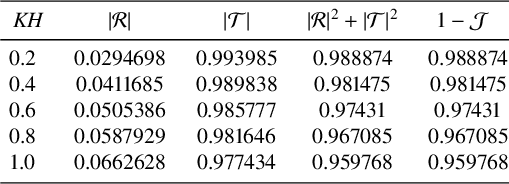
The validity of the energy balance relation presented in equation (5.1) is numerically verified in Table 1 for the flexible porous plates. This condition measures the energy dissipated due to the presence of porous elastic plates. The numerical consistency observed in Table 1 confirms the partial check of the current methodology.
Table 1 Values of $|\mathcal {R}|$
,
$|\mathcal {R}|$
, $|\mathcal {T}|$
,
$|\mathcal {T}|$
, $|\mathcal {R}|^2+ |\mathcal {T}|^2$
and
$|\mathcal {R}|^2+ |\mathcal {T}|^2$
and $1-\mathcal {J}$
for
$1-\mathcal {J}$
for $G=1+{{i}}$
,
$G=1+{{i}}$
, ${x_1}/{H}=2.65$
,
${x_1}/{H}=2.65$
, ${x_2}/{H}=2.55$
,
${x_2}/{H}=2.55$
, ${x_3}/{H}=2.45$
,
${x_3}/{H}=2.45$
, ${x_4}/{H}=2.35$
,
${x_4}/{H}=2.35$
, ${a_1}/{H}=0.65$
,
${a_1}/{H}=0.65$
, ${a_2}/{H}=0.45$
,
${a_2}/{H}=0.45$
, ${a_3}/{H}=0.35$
,
${a_3}/{H}=0.35$
, ${a_4}/{H}=0.55$
,
${a_4}/{H}=0.55$
, ${b_1}/{H}=0.95$
,
${b_1}/{H}=0.95$
, ${b_2}/{H}=0.55$
,
${b_2}/{H}=0.55$
, ${b_3}/{H}=0.55$
,
${b_3}/{H}=0.55$
, ${b_4}/{H}=0.70$
,
${b_4}/{H}=0.70$
, $m^f_p=0.01, D=0.4$
and
$m^f_p=0.01, D=0.4$
and $\beta =0.002$
.
$\beta =0.002$
.

Table 2 presents a convergence analysis of the infinite series by evaluating the reflection coefficients $|\mathcal {R}|$
for different truncation sizes
$|\mathcal {R}|$
for different truncation sizes $r = 20, 21, 22, 23, 24, 25$
across different values of
$r = 20, 21, 22, 23, 24, 25$
across different values of $KH$
. A nearly three-figure accuracy is attained by choosing
$KH$
. A nearly three-figure accuracy is attained by choosing $r=25$
, ensuring the convergence of the infinite series.
$r=25$
, ensuring the convergence of the infinite series.
Table 2 The reflection coefficients for ${x_1}/{H}=0.38,{x_2}/{H}=0.36,{x_3}/{H}=0.34, {x_4}/{H}=0.32$
,
${x_1}/{H}=0.38,{x_2}/{H}=0.36,{x_3}/{H}=0.34, {x_4}/{H}=0.32$
, ${a_1}/{H}=0.20$
,
${a_1}/{H}=0.20$
, ${a_2}/{H}=0.35$
,
${a_2}/{H}=0.35$
, ${a_3}/{H}=0.50$
,
${a_3}/{H}=0.50$
, ${a_4}/{H}=0.65$
,
${a_4}/{H}=0.65$
, ${b_1}/{H}=0.45$
,
${b_1}/{H}=0.45$
, ${b_2}/{H}=0.55$
,
${b_2}/{H}=0.55$
, ${b_3}/{H}=0.75$
,
${b_3}/{H}=0.75$
, ${b_4}/{H}=0.85$
,
${b_4}/{H}=0.85$
, $m^f_p=0.01$
,
$m^f_p=0.01$
, $D=0.4$
,
$D=0.4$
, $\beta =0.002$
,
$\beta =0.002$
, ${\lambda _1}/{H}=0.15$
,
${\lambda _1}/{H}=0.15$
, ${\lambda _2}/{H}=0.10$
,
${\lambda _2}/{H}=0.10$
, ${\lambda _3}/{H}=0.15$
and
${\lambda _3}/{H}=0.15$
and ${\lambda _4}/{H}=0.10$
.
${\lambda _4}/{H}=0.10$
.

To examine the convergence behaviour of the finite-term Galerkin expansion, the computed values of $|\mathcal {R}|$
,
$|\mathcal {R}|$
, $|\mathcal {T}|$
and
$|\mathcal {T}|$
and $\mathcal {J}$
for various numbers of terms
$\mathcal {J}$
for various numbers of terms $(M)$
in the multi-term Galerkin approximation are presented in Table 3. For this analysis, the parameters are selected as follows:
$(M)$
in the multi-term Galerkin approximation are presented in Table 3. For this analysis, the parameters are selected as follows: $G=0.75$
,
$G=0.75$
, ${x_1}/{H}=1.45$
,
${x_1}/{H}=1.45$
, ${x_2}/{H}=1.35$
,
${x_2}/{H}=1.35$
, ${x_3}/{H}=1.25$
,
${x_3}/{H}=1.25$
, ${x_4}/{H}=1.15$
,
${x_4}/{H}=1.15$
, ${a_1}/{H}=0.55$
,
${a_1}/{H}=0.55$
, ${a_2}/{H}=0.45$
,
${a_2}/{H}=0.45$
, ${a_3}/{H}=0.35$
,
${a_3}/{H}=0.35$
, ${a_4}/{H}=0.65$
,
${a_4}/{H}=0.65$
, ${b_1}/{H}=0.75$
,
${b_1}/{H}=0.75$
, ${b_2}/{H}=0.65$
,
${b_2}/{H}=0.65$
, ${b_3}/{H}=0.55$
,
${b_3}/{H}=0.55$
, ${b_4}/{H}=0.85$
,
${b_4}/{H}=0.85$
, $m^f_p=0.01$
,
$m^f_p=0.01$
, $D=0.4$
and
$D=0.4$
and $\beta =0.002$
. As presented in Table 3, an accuracy up to four significant figures (corresponding to an error estimate of
$\beta =0.002$
. As presented in Table 3, an accuracy up to four significant figures (corresponding to an error estimate of $10^{-5}$
) is attained for
$10^{-5}$
) is attained for $M=3$
(that is, four terms in the Galerkin approximation), thereby providing partial validation of the present study.
$M=3$
(that is, four terms in the Galerkin approximation), thereby providing partial validation of the present study.
Table 3 Convergence analysis of numerical estimates of $|\mathcal {R}|$
,
$|\mathcal {R}|$
, $|\mathcal {T}|$
and
$|\mathcal {T}|$
and $\mathcal {J}$
for varying numbers of terms (M) in the multi-term Galerkin approximation.
$\mathcal {J}$
for varying numbers of terms (M) in the multi-term Galerkin approximation.

6.2 Validation with existing results
Our present results are compared with those of Gupta and Gayen [Reference Gupta and Gayen14] for a dual porous plate, as shown in Figure 3, and with the results of Lee and Chwang [Reference Lee and Chwang19] for a single porous bottom-standing barrier in Figure 4.

Figure 3 $|\mathcal {R}|$
against
$|\mathcal {R}|$
against $KH$
for
$KH$
for ${x_1}/{H}=4.35$
,
${x_1}/{H}=4.35$
, ${x_2}/{H}=2.35001$
,
${x_2}/{H}=2.35001$
, ${x_3}/{H}=2.35001$
,
${x_3}/{H}=2.35001$
, ${x_4}/{H}=3.35$
,
${x_4}/{H}=3.35$
, ${a_1}/{H}=0.1$
,
${a_1}/{H}=0.1$
, ${a_2}/{H}=0.39999$
,
${a_2}/{H}=0.39999$
, ${a_3}/{H}=0.39999$
,
${a_3}/{H}=0.39999$
, ${a_4}/{H}=0.2$
,
${a_4}/{H}=0.2$
, ${b_1}/{H}=0.7$
,
${b_1}/{H}=0.7$
, ${b_2}/{H}=0.40001$
,
${b_2}/{H}=0.40001$
, ${b_3}/{H}=0.40001$
,
${b_3}/{H}=0.40001$
, ${b_4}/{H}=0.6$
,
${b_4}/{H}=0.6$
, $m^f_p=0.0001$
,
$m^f_p=0.0001$
, $D=0.9999$
and
$D=0.9999$
and $G=0.5(1+ {{i}})$
.
$G=0.5(1+ {{i}})$
.

Figure 4 $|\mathcal {R}|$
against
$|\mathcal {R}|$
against $KH$
for
$KH$
for $m^f_p = 0.0001$
,
$m^f_p = 0.0001$
, $D = 0.9999$
,
$D = 0.9999$
, ${b_1}/{H}={b_2}/{H}={b_3}/{H}={b_4}/{H}=1$
,
${b_1}/{H}={b_2}/{H}={b_3}/{H}={b_4}/{H}=1$
, ${a_1}/{H}=0.5$
,
${a_1}/{H}=0.5$
, ${a_2}/{H}=0.999$
,
${a_2}/{H}=0.999$
, ${a_3}/{H}=0.999$
,
${a_3}/{H}=0.999$
, ${a_4}/{H}=0.4$
,
${a_4}/{H}=0.4$
, ${x_1}/{H}=1.0$
,
${x_1}/{H}=1.0$
, ${x_2}/{H}=0.501$
,
${x_2}/{H}=0.501$
, ${x_3}/{H}=0.5001$
and
${x_3}/{H}=0.5001$
and ${x_4}/{H}=0.5$
.
${x_4}/{H}=0.5$
.
To replicate the configuration of two permeable plates in order to validate with Gupta and Gayen [Reference Gupta and Gayen14], we set $m^f_p = 0.0001$
and
$m^f_p = 0.0001$
and $D = 0.9999$
, effectively converting the porous elastic plates into purely permeable ones. Furthermore, to match the model configuration used by Gupta and Gayen [Reference Gupta and Gayen14], we adopt the following parameter values:
$D = 0.9999$
, effectively converting the porous elastic plates into purely permeable ones. Furthermore, to match the model configuration used by Gupta and Gayen [Reference Gupta and Gayen14], we adopt the following parameter values: ${x_1}/{H}=4.35$
,
${x_1}/{H}=4.35$
, ${x_2}/{H}=2.35001$
,
${x_2}/{H}=2.35001$
, ${x_3}/{H}=2.35001$
,
${x_3}/{H}=2.35001$
, ${x_4}/{H}=3.35$
,
${x_4}/{H}=3.35$
, ${a_1}/{H}=0.1$
,
${a_1}/{H}=0.1$
, ${a_2}/{H}=0.39999$
,
${a_2}/{H}=0.39999$
, ${a_3}/{H}=0.39999$
,
${a_3}/{H}=0.39999$
, ${a_4}/{H}=0.2$
,
${a_4}/{H}=0.2$
, ${b_1}/{H}=0.7$
,
${b_1}/{H}=0.7$
, ${b_2}/{H}=0.40001$
,
${b_2}/{H}=0.40001$
, ${b_3}/{H}=0.40001$
and
${b_3}/{H}=0.40001$
and ${b_4}/{H}=0.6$
. As shown in Figure 3, the reflection coefficient
${b_4}/{H}=0.6$
. As shown in Figure 3, the reflection coefficient $|\mathcal {R}|$
obtained from the present study aligns closely with the results obtained by Gupta and Gayen [Reference Gupta and Gayen14]. This validates the accuracy of the numerical approach employed in this work.
$|\mathcal {R}|$
obtained from the present study aligns closely with the results obtained by Gupta and Gayen [Reference Gupta and Gayen14]. This validates the accuracy of the numerical approach employed in this work.
Figure 4 shows the graph of the reflection coefficient $|\mathcal {R}|$
against
$|\mathcal {R}|$
against $KH$
for the case of a single bottom-standing permeable barrier. To adapt our model to this configuration, we set the parameters as follows:
$KH$
for the case of a single bottom-standing permeable barrier. To adapt our model to this configuration, we set the parameters as follows: $m^f_p = 0.0001$
,
$m^f_p = 0.0001$
, $D = 0.9999$
,
$D = 0.9999$
, ${b_j}/{H}=1$
,
${b_j}/{H}=1$
, $j=1,2,3,4$
,
$j=1,2,3,4$
, ${a_1}/{H}=0.5$
,
${a_1}/{H}=0.5$
, ${a_2}/{H}=0.999$
,
${a_2}/{H}=0.999$
, ${a_3}/{H}=0.999$
,
${a_3}/{H}=0.999$
, ${a_4}/{H}=0.4$
,
${a_4}/{H}=0.4$
, ${x_1}/{H}=1.0$
,
${x_1}/{H}=1.0$
, ${x_2}/{H}=0.501$
,
${x_2}/{H}=0.501$
, ${x_3}/{H}=0.5001$
,
${x_3}/{H}=0.5001$
, ${x_4}/{H}=0.5$
. As apparent from Figure 4, the curves of
${x_4}/{H}=0.5$
. As apparent from Figure 4, the curves of $|\mathcal {R}|$
closely match the corresponding results from Lee and Chwang [Reference Lee and Chwang19]. This agreement validates the accuracy of the present work.
$|\mathcal {R}|$
closely match the corresponding results from Lee and Chwang [Reference Lee and Chwang19]. This agreement validates the accuracy of the present work.
Table 4 presents a validation of the present results against those obtained by Chakraborty and Mandal [Reference Chakraborty and Mandal3] and by Mandal and Dolai [Reference Mandal and Dolai24] for a single rigid thin vertical submerged plate. For the parameter values $KH=0.2$
,
$KH=0.2$
, $m^f_p=0.0001$
,
$m^f_p=0.0001$
, ${D=0.9999}$
,
${D=0.9999}$
, $G=0$
,
$G=0$
, ${x_1}/{H}=0.001$
,
${x_1}/{H}=0.001$
, ${x_2}/{H}=0.0001$
,
${x_2}/{H}=0.0001$
, ${x_3}/{H}=0.00001$
,
${x_3}/{H}=0.00001$
, ${x_4}/{H}=0.000001$
,
${x_4}/{H}=0.000001$
, ${a_1}/{H}=0.2$
,
${a_1}/{H}=0.2$
, ${a_2}/{H}=0.199$
,
${a_2}/{H}=0.199$
, ${a_3}/{H}=0.1999$
,
${a_3}/{H}=0.1999$
, ${a_4}/{H}=0.19999$
,
${a_4}/{H}=0.19999$
, ${b_2}/{H}=0.201$
,
${b_2}/{H}=0.201$
, ${b_3}/{H}=0.2001$
,
${b_3}/{H}=0.2001$
, ${b_4}/{H}=0.20001$
and
${b_4}/{H}=0.20001$
and $\beta =0$
, the four porous flexible plates considered in the present model effectively reduce to a single thin rigid plate, as in the configurations studied by Chakraborty and Mandal [Reference Chakraborty and Mandal3] and Mandal and Dolai [Reference Mandal and Dolai24]. The present results exhibit excellent agreement, with accuracy up to three decimal places, thereby validating the numerical accuracy of the proposed method.
$\beta =0$
, the four porous flexible plates considered in the present model effectively reduce to a single thin rigid plate, as in the configurations studied by Chakraborty and Mandal [Reference Chakraborty and Mandal3] and Mandal and Dolai [Reference Mandal and Dolai24]. The present results exhibit excellent agreement, with accuracy up to three decimal places, thereby validating the numerical accuracy of the proposed method.
Table 4 The reflection coefficient $|\mathcal {R}|$
against
$|\mathcal {R}|$
against ${b_1}/{H}$
for
${b_1}/{H}$
for $KH=0.2, m^f_p=0.0001, D=0.9999$
,
$KH=0.2, m^f_p=0.0001, D=0.9999$
, $G=0$
,
$G=0$
, ${x_1}/{H}=0.001, {x_2}/{H}=0.0001, {x_3}/{H}=0.00001,{x_4}/{H}=0.000001, {a_1}/{H}=0.2, {a_2}/{H}=0.199, {a_3}/{H}=0.1999$
,
${x_1}/{H}=0.001, {x_2}/{H}=0.0001, {x_3}/{H}=0.00001,{x_4}/{H}=0.000001, {a_1}/{H}=0.2, {a_2}/{H}=0.199, {a_3}/{H}=0.1999$
, ${a_4}/{H}=0.19999, {b_2}/{H}=0.201$
,
${a_4}/{H}=0.19999, {b_2}/{H}=0.201$
, ${b_3}/{H}=0.2001$
,
${b_3}/{H}=0.2001$
, ${b_4}/{H}=0.20001$
and
${b_4}/{H}=0.20001$
and $\beta =0$
.
$\beta =0$
.

6.3 Influence of key parameters on hydrodynamic quantities of the submerged plates
6.3.1 Significance of different number of plates
Figure 5 depicts the graphical representation of reflection, transmission coefficients, dissipated wave energy and hydrodynamic force against wave number $KH$
, considering different numbers of flexible porous plates. The parameter values selected for different plate configurations are presented in Table 5. For the four-plate configuration, we use the values listed under
$KH$
, considering different numbers of flexible porous plates. The parameter values selected for different plate configurations are presented in Table 5. For the four-plate configuration, we use the values listed under $N=4$
. This set-up reduces to a three-plate configuration when the values under
$N=4$
. This set-up reduces to a three-plate configuration when the values under $N=3$
are considered. Similarly, for the two-plate set-up, the parameters corresponding to
$N=3$
are considered. Similarly, for the two-plate set-up, the parameters corresponding to $N=2$
are used. Finally, when
$N=2$
are used. Finally, when $N=1$
, the two-plate configuration simplifies to a single-plate set-up. The other parameters are kept fixed at
$N=1$
, the two-plate configuration simplifies to a single-plate set-up. The other parameters are kept fixed at $ G=0.5, m^f_p=0.01, D=0.4$
and
$ G=0.5, m^f_p=0.01, D=0.4$
and $\beta =0.002$
for each arrangement. As observed in Figure 5(a), an increase in the number of submerged plates results in a significant enhancement of the reflection coefficient amplitude. Moreover,
$\beta =0.002$
for each arrangement. As observed in Figure 5(a), an increase in the number of submerged plates results in a significant enhancement of the reflection coefficient amplitude. Moreover, $|\mathcal {R}|$
exhibits increasingly oscillatory characteristics with the addition of more barriers, indicating complex wave interaction and multiple scattering effects. Figure 5(b) illustrates that increasing the number of plates in the breakwater system leads to a reduction in transmitted wave energy, whereas Figure 5(c) demonstrates a corresponding increase in the dissipated wave energy. Figure 5(d) indicates that the oscillatory nature of the hydrodynamic force intensifies as the number of plates increases. The curves corresponding to higher plate counts
$|\mathcal {R}|$
exhibits increasingly oscillatory characteristics with the addition of more barriers, indicating complex wave interaction and multiple scattering effects. Figure 5(b) illustrates that increasing the number of plates in the breakwater system leads to a reduction in transmitted wave energy, whereas Figure 5(c) demonstrates a corresponding increase in the dissipated wave energy. Figure 5(d) indicates that the oscillatory nature of the hydrodynamic force intensifies as the number of plates increases. The curves corresponding to higher plate counts $(N=3, N=4)$
exhibit greater amplitude fluctuations than those with fewer plates
$(N=3, N=4)$
exhibit greater amplitude fluctuations than those with fewer plates $(N=1, N=2)$
across all
$(N=1, N=2)$
across all $KH$
values.
$KH$
values.
Table 5 Parameter values for different plate configurations.


Figure 5 Graphs of (a) $|\mathcal {R}|$
, (b)
$|\mathcal {R}|$
, (b) $|\mathcal {T}|$
, (c)
$|\mathcal {T}|$
, (c) $\mathcal {J}$
and (d)
$\mathcal {J}$
and (d) $\mathcal {H}^f$
against
$\mathcal {H}^f$
against $KH$
for different number of plates with fixed
$KH$
for different number of plates with fixed $ G=0.5, m^f_p=0.01, D=0.4$
and
$ G=0.5, m^f_p=0.01, D=0.4$
and $\beta =0.002$
.
$\beta =0.002$
.
These observations suggest that adding more plates not only suppresses wave transmission but also promotes reflection and energy dissipation, thereby improving the overall effectiveness of the breakwater system. Furthermore, systems with a large number of plates exhibit stronger variability in hydrodynamic forces. Therefore, $N=4$
provides better results than other barrier configurations, and hence four barriers are considered in the subsequent parametric analysis.
$N=4$
provides better results than other barrier configurations, and hence four barriers are considered in the subsequent parametric analysis.
6.3.2 Effect of porosity parameter
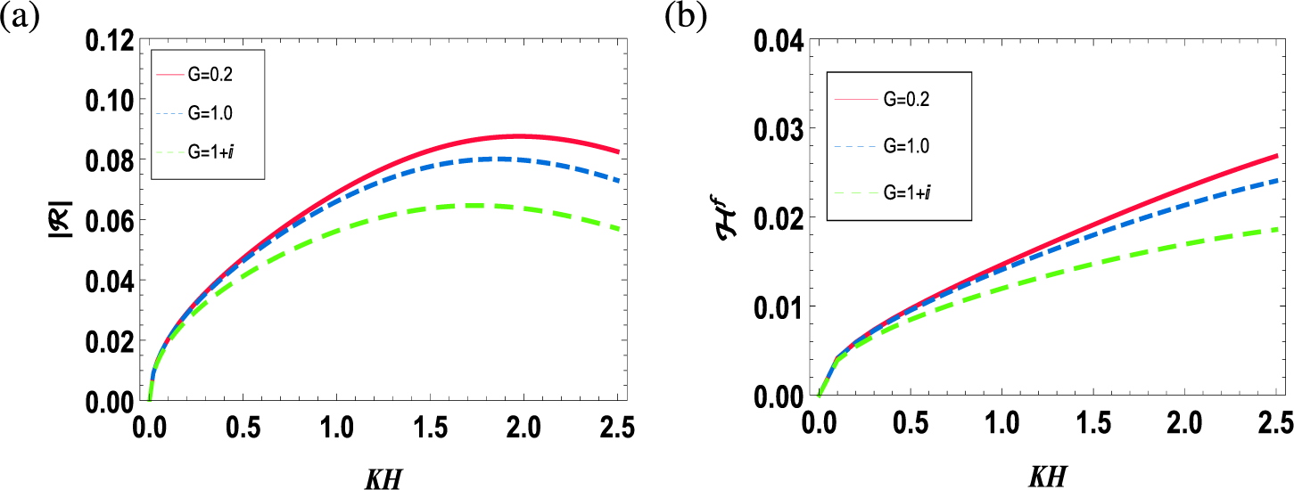
Figures 6 and 7 highlight the variations in reflection coefficient and hydrodynamic force for varying porosity parameter, considering both uniform and nonuniform porosity distributions.

Figure 6 Graphs of (a) $|\mathcal {R}|$
and (b)
$|\mathcal {R}|$
and (b) $\mathcal {H}^f$
against
$\mathcal {H}^f$
against $KH$
for different values of porosity with
$KH$
for different values of porosity with ${x_1}/{H}=1.45$
,
${x_1}/{H}=1.45$
, ${x_2}/{H}=1.35$
,
${x_2}/{H}=1.35$
, ${x_3}/{H}=1.25$
,
${x_3}/{H}=1.25$
, ${x_4}/{H}=1.15$
,
${x_4}/{H}=1.15$
, ${a_1}/{H}=0.55$
,
${a_1}/{H}=0.55$
, ${a_2}/{H}=0.45$
,
${a_2}/{H}=0.45$
, ${a_3}/{H}=0.35$
,
${a_3}/{H}=0.35$
, ${a_4}/{H}$
,
${a_4}/{H}$
, $=0.65$
,
$=0.65$
, ${b_1}/{H}=0.75$
,
${b_1}/{H}=0.75$
, ${b_2}/{H}=0.65$
,
${b_2}/{H}=0.65$
, ${b_3}/{H}=0.55$
,
${b_3}/{H}=0.55$
, ${b_4}/{H}=0.85$
,
${b_4}/{H}=0.85$
, $m^f_p=0.01$
,
$m^f_p=0.01$
, $D=0.4$
and
$D=0.4$
and $\beta =0.002$
.
$\beta =0.002$
.

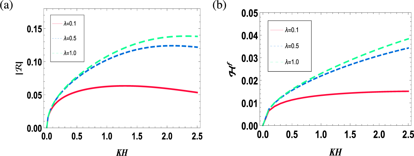
Figure 7 Graphs of (a) $|\mathcal {R}|$
and (b)
$|\mathcal {R}|$
and (b) $\mathcal {H}^f$
against
$\mathcal {H}^f$
against $KH$
for different values of
$KH$
for different values of $\lambda $
with
$\lambda $
with ${x_1}/{H}=0.5$
,
${x_1}/{H}=0.5$
, ${x_2}/{H}=0.4$
,
${x_2}/{H}=0.4$
, ${x_3}/{H}=0.3$
,
${x_3}/{H}=0.3$
, ${x_4}/{H}=0.2$
,
${x_4}/{H}=0.2$
, ${a_1}/{H}=0.35$
,
${a_1}/{H}=0.35$
, ${a_2}/{H}=0.25$
,
${a_2}/{H}=0.25$
, ${a_3}/{H}=0.45$
,
${a_3}/{H}=0.45$
, ${a_4}/{H} =0.75$
,
${a_4}/{H} =0.75$
, ${b_1}/{H} =0.65$
,
${b_1}/{H} =0.65$
, ${b_2}/{H}=0.45$
,
${b_2}/{H}=0.45$
, ${b_3}/{H}=0.75$
,
${b_3}/{H}=0.75$
, ${b_4}/{H}=0.95$
,
${b_4}/{H}=0.95$
, $m^f_p=0.01$
,
$m^f_p=0.01$
, $D=0.4$
and
$D=0.4$
and $\beta = 0.002$
.
$\beta = 0.002$
.
In Figure 6, $|\mathcal {R}|$
and
$|\mathcal {R}|$
and $\mathcal {H}^f$
are plotted against nondimensional wave number
$\mathcal {H}^f$
are plotted against nondimensional wave number $KH$
for different values of uniform porosity
$KH$
for different values of uniform porosity $G=0.2, 1.0, 1+ {{i}}$
. The other parameters are fixed at
$G=0.2, 1.0, 1+ {{i}}$
. The other parameters are fixed at ${x_1}/{H}=1.45$
,
${x_1}/{H}=1.45$
, ${x_2}/{H}=1.35$
,
${x_2}/{H}=1.35$
, ${x_3}/{H}=1.25$
,
${x_3}/{H}=1.25$
, ${x_4}/{H}=1.15$
,
${x_4}/{H}=1.15$
, ${a_1}/{H}=0.55$
,
${a_1}/{H}=0.55$
, ${a_2}/{H}=0.45$
,
${a_2}/{H}=0.45$
, ${a_3}/{H}=0.35$
,
${a_3}/{H}=0.35$
, ${a_4}/{H}=0.65$
,
${a_4}/{H}=0.65$
, ${b_1}/{H}=0.75$
,
${b_1}/{H}=0.75$
, ${b_2}/{H}=0.65$
,
${b_2}/{H}=0.65$
, ${b_3}/{H}=0.55$
,
${b_3}/{H}=0.55$
, ${b_4}/{H}=0.85$
,
${b_4}/{H}=0.85$
, $m^f_p=0.01$
,
$m^f_p=0.01$
, $D=0.4$
and
$D=0.4$
and $\beta =0.002$
. Figure 6 shows that both the reflected energy and the wave-induced force decrease as the magnitude of uniform porosity increases. This observation suggests that increased porosity enhances energy absorption within the porous material, leading to diminished wave reflection and lower hydrodynamic forces on the structure. This underscores the role of porous materials in wave energy attenuation and load mitigation.
$\beta =0.002$
. Figure 6 shows that both the reflected energy and the wave-induced force decrease as the magnitude of uniform porosity increases. This observation suggests that increased porosity enhances energy absorption within the porous material, leading to diminished wave reflection and lower hydrodynamic forces on the structure. This underscores the role of porous materials in wave energy attenuation and load mitigation.
Figure 7 shows the variation of $|\mathcal {R}|$
and
$|\mathcal {R}|$
and $\mathcal {H}^f$
with respect to the parameter
$\mathcal {H}^f$
with respect to the parameter $\lambda $
which is inversely proportional to the porosity parameter. In this configuration, we choose
$\lambda $
which is inversely proportional to the porosity parameter. In this configuration, we choose ${x_1}/{H}=0.5$
,
${x_1}/{H}=0.5$
, ${x_2}/{H}=0.4$
,
${x_2}/{H}=0.4$
, ${x_3}/{H}=0.3$
,
${x_3}/{H}=0.3$
, ${x_4}/{H}=0.2$
,
${x_4}/{H}=0.2$
, ${a_1}/{H}=0.35$
,
${a_1}/{H}=0.35$
, ${a_2}/{H}=0.25$
,
${a_2}/{H}=0.25$
, ${a_3}/{H}=0.45$
,
${a_3}/{H}=0.45$
, ${a_4}/{H}=0.75$
,
${a_4}/{H}=0.75$
, ${b_1}/{H}=0.65$
,
${b_1}/{H}=0.65$
, ${b_2}/{H}=0.45$
,
${b_2}/{H}=0.45$
, ${b_3}/{H}=0.75$
,
${b_3}/{H}=0.75$
, ${b_4}/{H}=0.95$
,
${b_4}/{H}=0.95$
, $m^f_p=0.01$
,
$m^f_p=0.01$
, $D=0.4$
and
$D=0.4$
and $\beta = 0.002$
. As
$\beta = 0.002$
. As $\lambda $
decreases (porosity increases), the reflection coefficient
$\lambda $
decreases (porosity increases), the reflection coefficient $|\mathcal {R}|$
and wave-induced force
$|\mathcal {R}|$
and wave-induced force $\mathcal {H}^f$
on the plate decrease. This indicates that higher porosity allows more fluid flow through the pores, enhancing energy dissipation within the medium. As a result, less wave energy is reflected, and the dynamic loading on the structure is reduced.
$\mathcal {H}^f$
on the plate decrease. This indicates that higher porosity allows more fluid flow through the pores, enhancing energy dissipation within the medium. As a result, less wave energy is reflected, and the dynamic loading on the structure is reduced.
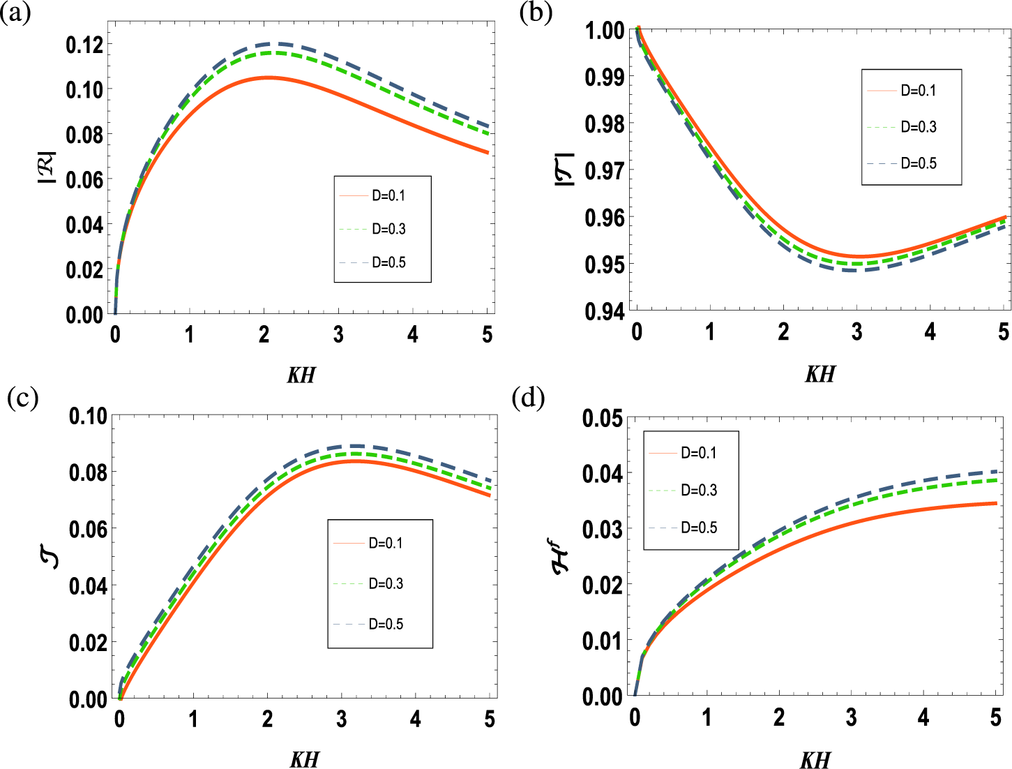
6.3.3 Influence of flexural rigidity
Figure 8 portrays the impact of the plate’s flexural rigidity on various hydrodynamic parameters, including $|\mathcal {R}|$
,
$|\mathcal {R}|$
, $|\mathcal {T}|$
,
$|\mathcal {T}|$
, $\mathcal {J}$
and
$\mathcal {J}$
and $\mathcal {H}^f$
, plotted as a function of
$\mathcal {H}^f$
, plotted as a function of $KH$
. The analysis is conducted using the parameters
$KH$
. The analysis is conducted using the parameters $G=0.5+ 0.5{{i}}$
,
$G=0.5+ 0.5{{i}}$
, ${x_1}/{H}=0.5$
,
${x_1}/{H}=0.5$
, ${x_2}/{H}=0.4$
,
${x_2}/{H}=0.4$
, ${x_3}/{H}=0.3$
,
${x_3}/{H}=0.3$
, ${x_4}/{H}=0.2$
,
${x_4}/{H}=0.2$
, ${a_1}/{H}=0.35$
,
${a_1}/{H}=0.35$
, ${a_2}/{H}=0.25$
,
${a_2}/{H}=0.25$
, ${a_3}/{H}=0.45$
,
${a_3}/{H}=0.45$
, ${a_4}/{H}=0.75$
,
${a_4}/{H}=0.75$
, ${b_1}/{H}=0.65$
,
${b_1}/{H}=0.65$
, ${b_2}/{H}=0.45$
,
${b_2}/{H}=0.45$
, ${b_3}/{H}=0.75$
,
${b_3}/{H}=0.75$
, ${b_4}/{H}=0.95$
,
${b_4}/{H}=0.95$
, $m^f_p=0.01$
and
$m^f_p=0.01$
and $\beta = 0.002$
. It is observed from Figure 8 that
$\beta = 0.002$
. It is observed from Figure 8 that $|\mathcal {R}|$
,
$|\mathcal {R}|$
, $\mathcal {J}$
and
$\mathcal {J}$
and $\mathcal {H}^f$
increase while
$\mathcal {H}^f$
increase while $|\mathcal {T}|$
decreases with increasing values of flexural rigidity D. Flexural rigidity reflects a plate’s resistance to bending: as it increases, the plate becomes stiffer. This enhanced stiffness leads to greater energy reflection, reduced energy transmission, and consequently, increased energy dissipation and hydrodynamic force.
$|\mathcal {T}|$
decreases with increasing values of flexural rigidity D. Flexural rigidity reflects a plate’s resistance to bending: as it increases, the plate becomes stiffer. This enhanced stiffness leads to greater energy reflection, reduced energy transmission, and consequently, increased energy dissipation and hydrodynamic force.

Figure 8 Graphs of (a) $|\mathcal {R}|$
, (b)
$|\mathcal {R}|$
, (b) $|\mathcal {T}|$
, (c)
$|\mathcal {T}|$
, (c) $\mathcal {J}$
and (d)
$\mathcal {J}$
and (d) $\mathcal {H}^f$
against
$\mathcal {H}^f$
against $KH$
for different values of flexural rigidity with
$KH$
for different values of flexural rigidity with $G=0.5+ 0.5{{i}}$
,
$G=0.5+ 0.5{{i}}$
, ${x_1}/{H}=0.5$
,
${x_1}/{H}=0.5$
, ${x_2}/{H}=0.4$
,
${x_2}/{H}=0.4$
, ${x_3}/{H}=0.3$
,
${x_3}/{H}=0.3$
, ${x_4}/{H}=0.2$
,
${x_4}/{H}=0.2$
, ${a_1}/{H}=0.35$
,
${a_1}/{H}=0.35$
, ${a_2}/{H}=0.25$
,
${a_2}/{H}=0.25$
, ${a_3}/{H}=0.45$
,
${a_3}/{H}=0.45$
, ${a_4}/{H}=0.75$
,
${a_4}/{H}=0.75$
, ${b_1}/{H}=0.65$
,
${b_1}/{H}=0.65$
, ${b_2}/{H}=0.45$
,
${b_2}/{H}=0.45$
, ${b_3}/{H}=0.75$
,
${b_3}/{H}=0.75$
, ${b_4}/{H}=0.95$
,
${b_4}/{H}=0.95$
, $m^f_p=0.01$
and
$m^f_p=0.01$
and $\beta = 0.002$
.
$\beta = 0.002$
.
6.3.4 Impact of ice sheet thickness
The influence of ice sheet thickness on the reflection coefficient ( $|\mathcal {R}|$
), transmission coefficient (
$|\mathcal {R}|$
), transmission coefficient ( $|\mathcal {T}|$
), dissipated energy (
$|\mathcal {T}|$
), dissipated energy ( $\mathcal {J}$
), and horizontal wave force (
$\mathcal {J}$
), and horizontal wave force ( $\mathcal {H}^f$
) is illustrated in Figure 9 for various thickness ratios
$\mathcal {H}^f$
) is illustrated in Figure 9 for various thickness ratios $\beta = {h}/{H} = 0.002,~0.01,~0.02$
. The remaining parameters are fixed as
$\beta = {h}/{H} = 0.002,~0.01,~0.02$
. The remaining parameters are fixed as $G = 0.5$
,
$G = 0.5$
, ${x_1}/{H} = 1.45$
,
${x_1}/{H} = 1.45$
, ${x_2}/{H} = 1.35$
,
${x_2}/{H} = 1.35$
, ${x_3}/{H} = 1.25$
,
${x_3}/{H} = 1.25$
, ${x_4}/{H} = 1.15$
,
${x_4}/{H} = 1.15$
, ${a_1}/{H} = 0.55$
,
${a_1}/{H} = 0.55$
, ${a_2}/{H} = 0.45$
,
${a_2}/{H} = 0.45$
, ${a_3}/{H} = 0.35$
,
${a_3}/{H} = 0.35$
, ${a_4}/{H} = 0.65$
,
${a_4}/{H} = 0.65$
, ${b_1}/{H} = 0.75$
,
${b_1}/{H} = 0.75$
, ${b_2}/{H} = 0.65$
,
${b_2}/{H} = 0.65$
, ${b_3}/{H} = 0.55$
,
${b_3}/{H} = 0.55$
, ${b_4}/{H} = 0.85$
,
${b_4}/{H} = 0.85$
, $m^f_p = 0.01$
, and
$m^f_p = 0.01$
, and $D = 0.4$
. Figures 9(a)–9(d) reveal that in case of low wave number (
$D = 0.4$
. Figures 9(a)–9(d) reveal that in case of low wave number ( $KH < 0.45$
), variations in ice thickness have a negligible impact on wave behaviour, indicating weak ice–wave interaction. However, for shorter waves (
$KH < 0.45$
), variations in ice thickness have a negligible impact on wave behaviour, indicating weak ice–wave interaction. However, for shorter waves ( $KH> 0.45$
), the influence of ice becomes increasingly significant. An increase in
$KH> 0.45$
), the influence of ice becomes increasingly significant. An increase in $\beta $
leads to a reduction in reflected wave energy (
$\beta $
leads to a reduction in reflected wave energy ( $|\mathcal {R}|$
), dissipated energy (
$|\mathcal {R}|$
), dissipated energy ( $\mathcal {J}$
), and wave-induced force (
$\mathcal {J}$
), and wave-induced force ( $\mathcal {H}^f$
), while the transmitted energy (
$\mathcal {H}^f$
), while the transmitted energy ( $|\mathcal {T}|$
) increases. Figures 9(a) and 9(c) highlight that
$|\mathcal {T}|$
) increases. Figures 9(a) and 9(c) highlight that $|\mathcal {R}|$
and
$|\mathcal {R}|$
and $\mathcal {J}$
initially rise, reach a peak, and then decrease, underscoring that thinner ice sheets enhance wave reflection and energy dissipation. Meanwhile, the transmission coefficient in Figure 9(b) shows a complementary trend, with thicker ice permitting more wave energy to pass through. The wave-induced force (
$\mathcal {J}$
initially rise, reach a peak, and then decrease, underscoring that thinner ice sheets enhance wave reflection and energy dissipation. Meanwhile, the transmission coefficient in Figure 9(b) shows a complementary trend, with thicker ice permitting more wave energy to pass through. The wave-induced force ( $\mathcal {H}^f$
) in Figure 9(d) monotonically increases with
$\mathcal {H}^f$
) in Figure 9(d) monotonically increases with $KH$
, demonstrating that shorter waves exert greater hydrodynamic forces on the ice sheet. The figures also reveal that wave energy dissipation and hydrodynamic forces are more pronounced for thinner ice sheets, as their reduced rigidity enhances dynamic interactions with incoming waves.
$KH$
, demonstrating that shorter waves exert greater hydrodynamic forces on the ice sheet. The figures also reveal that wave energy dissipation and hydrodynamic forces are more pronounced for thinner ice sheets, as their reduced rigidity enhances dynamic interactions with incoming waves.

Figure 9 Graphs of (a) $|\mathcal {R}|$
, (b)
$|\mathcal {R}|$
, (b) $|\mathcal {T}|$
, (c)
$|\mathcal {T}|$
, (c) $\mathcal {J}$
and (d)
$\mathcal {J}$
and (d) $\mathcal {H}^f$
against
$\mathcal {H}^f$
against $KH$
for different values of ice sheet thickness with fixed
$KH$
for different values of ice sheet thickness with fixed $G=0.5$
,
$G=0.5$
, ${x_1}/{H}=1.45$
,
${x_1}/{H}=1.45$
, ${x_2}/{H}=1.35$
,
${x_2}/{H}=1.35$
, ${x_3}/{H}=1.25$
,
${x_3}/{H}=1.25$
, ${x_4}/{H}=1.15$
,
${x_4}/{H}=1.15$
, ${a_1}/{H}=0.55$
,
${a_1}/{H}=0.55$
, ${a_2}/{H}=0.45$
,
${a_2}/{H}=0.45$
, ${a_3}/{H}=0.35$
,
${a_3}/{H}=0.35$
, ${a_4}/{H}=0.65$
,
${a_4}/{H}=0.65$
, ${b_1}/{H}=0.75$
,
${b_1}/{H}=0.75$
, ${b_2}/{H}=0.65$
,
${b_2}/{H}=0.65$
, $ {b_3}/{H}=0.55$
,
$ {b_3}/{H}=0.55$
, ${b_4}/{H} =0.85$
,
${b_4}/{H} =0.85$
, $m^f_p=0.01$
and
$m^f_p=0.01$
and $D=0.4$
.
$D=0.4$
.
6.3.5 Influence of separation length between the submerged plates
Figure 10 illustrates the variations of $|\mathcal {R}|$
,
$|\mathcal {R}|$
, $|\mathcal {T}|$
,
$|\mathcal {T}|$
, $\mathcal {J}$
, and
$\mathcal {J}$
, and $\mathcal {H}^f$
with respect to the wave number
$\mathcal {H}^f$
with respect to the wave number $KH$
for different separation lengths between the plates, while keeping the following parameters fixed:
$KH$
for different separation lengths between the plates, while keeping the following parameters fixed: ${a_1}/{H}=0.50$
,
${a_1}/{H}=0.50$
, ${a_2}/{H}=0.45$
,
${a_2}/{H}=0.45$
, ${a_3}/{H}=0.35$
,
${a_3}/{H}=0.35$
, ${a_4}/{H}=0.65$
,
${a_4}/{H}=0.65$
, ${b_1}/{H}=0.75$
,
${b_1}/{H}=0.75$
, ${b_2}/{H}{\kern-1.5pt}={\kern-1.5pt}0.85$
,
${b_2}/{H}{\kern-1.5pt}={\kern-1.5pt}0.85$
, ${b_3}/{H}{\kern-1.5pt}={\kern-1.5pt}0.65$
,
${b_3}/{H}{\kern-1.5pt}={\kern-1.5pt}0.65$
, ${b_4}/{H}{\kern-1.5pt}={\kern-1.5pt}0.95$
,
${b_4}/{H}{\kern-1.5pt}={\kern-1.5pt}0.95$
, $m^f_p{\kern-1.5pt}={\kern-1.5pt}0.01$
,
$m^f_p{\kern-1.5pt}={\kern-1.5pt}0.01$
, $D{\kern-1.5pt}={\kern-1.5pt}0.4$
,
$D{\kern-1.5pt}={\kern-1.5pt}0.4$
, $\beta {\kern-1.5pt}={\kern-1.5pt}0.002$
,
$\beta {\kern-1.5pt}={\kern-1.5pt}0.002$
, ${\lambda _1}/{H}=0.25$
,
${\lambda _1}/{H}=0.25$
, ${\lambda _2}/{H}=0.35$
,
${\lambda _2}/{H}=0.35$
, ${\lambda _3}/{H}=0.25$
and
${\lambda _3}/{H}=0.25$
and ${\lambda _4}/{H}=0.35$
. It is observed from Figure 10(a) that, when the plates are closely spaced, the reflection is strong and smooth. However, as the spacing between the plates increases, the peak value of
${\lambda _4}/{H}=0.35$
. It is observed from Figure 10(a) that, when the plates are closely spaced, the reflection is strong and smooth. However, as the spacing between the plates increases, the peak value of $|\mathcal {R}|$
decreases, and an oscillatory nature emerges, which becomes more pronounced for widely spaced submerged plates due to interference effects. Moreover, for small
$|\mathcal {R}|$
decreases, and an oscillatory nature emerges, which becomes more pronounced for widely spaced submerged plates due to interference effects. Moreover, for small $KH < 0.5$
, the differences among configurations are negligible, but as
$KH < 0.5$
, the differences among configurations are negligible, but as $KH$
increases,
$KH$
increases, $|\mathcal {R}|$
rises, peaks, and then oscillates with further increases in
$|\mathcal {R}|$
rises, peaks, and then oscillates with further increases in $KH$
. Larger separations shift the reflection peak to lower
$KH$
. Larger separations shift the reflection peak to lower $KH$
values and reduce its magnitude, while shorter separations yield stronger reflection at mid-range wave numbers. Figures 10(b) and 10(c) show that the peak values of the transmission coefficient (
$KH$
values and reduce its magnitude, while shorter separations yield stronger reflection at mid-range wave numbers. Figures 10(b) and 10(c) show that the peak values of the transmission coefficient ( $|\mathcal {T}|$
) decrease, while energy dissipation (
$|\mathcal {T}|$
) decrease, while energy dissipation ( $\mathcal {J}$
) increases with greater separation between the plates. As
$\mathcal {J}$
) increases with greater separation between the plates. As $KH$
increases,
$KH$
increases, $|\mathcal {T}|$
gradually declines, reaching a minimum around
$|\mathcal {T}|$
gradually declines, reaching a minimum around $KH\approx 2.5$
, before rising again, indicating that wave transmission is highest for long waves and slightly reduced for intermediate wave numbers. In contrast, Figure 10(c) shows that
$KH\approx 2.5$
, before rising again, indicating that wave transmission is highest for long waves and slightly reduced for intermediate wave numbers. In contrast, Figure 10(c) shows that $\mathcal {J}$
is minimal for low
$\mathcal {J}$
is minimal for low $KH$
and increases monotonically with rising
$KH$
and increases monotonically with rising $KH$
, suggesting enhanced energy dissipation at higher wave numbers. In both cases, differences between the configurations are negligible for
$KH$
, suggesting enhanced energy dissipation at higher wave numbers. In both cases, differences between the configurations are negligible for ${KH<1.0}$
but become increasingly significant at higher values, highlighting the growing impact of plate spacing on wave transmission and energy dissipation. Finally, Figure 10(d) reveals that increasing the spacing between the plates significantly reduces the hydrodynamic force (
${KH<1.0}$
but become increasingly significant at higher values, highlighting the growing impact of plate spacing on wave transmission and energy dissipation. Finally, Figure 10(d) reveals that increasing the spacing between the plates significantly reduces the hydrodynamic force ( $\mathcal {H}^f$
) exerted by the waves, especially for higher wave numbers.
$\mathcal {H}^f$
) exerted by the waves, especially for higher wave numbers.

Figure 10 Graphs of (a) $|\mathcal {R}|$
, (b)
$|\mathcal {R}|$
, (b) $|\mathcal {T}|$
, (c)
$|\mathcal {T}|$
, (c) $\mathcal {J}$
and (d)
$\mathcal {J}$
and (d) $\mathcal {H}^f$
against
$\mathcal {H}^f$
against $KH$
for different values of separation length with
$KH$
for different values of separation length with ${a_1}/{H}=0.50$
,
${a_1}/{H}=0.50$
, $ {a_2}/{H}=0.45$
,
$ {a_2}/{H}=0.45$
, ${a_3}/{H}=0.35$
,
${a_3}/{H}=0.35$
, ${a_4}/{H}=0.65$
,
${a_4}/{H}=0.65$
, ${b_1}/{H}=0.75$
,
${b_1}/{H}=0.75$
, ${b_2}/{H}=0.85$
,
${b_2}/{H}=0.85$
, ${b_3}/{H} =0.65$
,
${b_3}/{H} =0.65$
, ${b_4}/{H}=0.95$
,
${b_4}/{H}=0.95$
, $m^f_p=0.01$
,
$m^f_p=0.01$
, $D=0.4$
,
$D=0.4$
, $\beta =0.002$
,
$\beta =0.002$
, ${\lambda _1}/{H}=0.25$
,
${\lambda _1}/{H}=0.25$
, ${\lambda _2}/{H}=0.35$
,
${\lambda _2}/{H}=0.35$
, ${\lambda _3}/{H}=0.25$
and
${\lambda _3}/{H}=0.25$
and ${\lambda _4}/{H}=0.35 $
.
${\lambda _4}/{H}=0.35 $
.
6.3.6 Effect of plate length
Figure 11 showcases the effect of different plate lengths on the hydrodynamic quantities $|\mathcal {R}|$
,
$|\mathcal {R}|$
, $|\mathcal {T}|$
,
$|\mathcal {T}|$
, $\mathcal {J}$
, and
$\mathcal {J}$
, and $\mathcal {H}^f$
with fixed
$\mathcal {H}^f$
with fixed ${G= 1+0.5{{i}}}$
,
${G= 1+0.5{{i}}}$
, ${x_1}/{H}=4.85$
,
${x_1}/{H}=4.85$
, ${x_2}/{H}=4.65$
,
${x_2}/{H}=4.65$
, ${x_3}/{H}=4.45$
,
${x_3}/{H}=4.45$
, ${x_4}/{H}=4.25$
,
${x_4}/{H}=4.25$
, $m^f_p=0.01$
,
$m^f_p=0.01$
, $D=0.4$
and
$D=0.4$
and ${\beta =0.002}$
. The results reveal that
${\beta =0.002}$
. The results reveal that $|\mathcal {R}|$
,
$|\mathcal {R}|$
, $\mathcal {J}$
and
$\mathcal {J}$
and $\mathcal {H}^f$
increase with increasing plate length, while
$\mathcal {H}^f$
increase with increasing plate length, while $|\mathcal {T}|$
decreases. Physically, this means that a longer plate reflects more of the incident wave energy, while allowing less to transmit through. The growth in
$|\mathcal {T}|$
decreases. Physically, this means that a longer plate reflects more of the incident wave energy, while allowing less to transmit through. The growth in $\mathcal {J}$
suggests enhanced energy dissipation, meaning longer plates absorb more wave energy. Similarly, the increase in
$\mathcal {J}$
suggests enhanced energy dissipation, meaning longer plates absorb more wave energy. Similarly, the increase in $\mathcal {H}^f$
reflects greater hydrodynamic loading on longer plates. As
$\mathcal {H}^f$
reflects greater hydrodynamic loading on longer plates. As $KH$
increases,
$KH$
increases, $|\mathcal {R}|$
,
$|\mathcal {R}|$
, $\mathcal {J}$
and
$\mathcal {J}$
and $\mathcal {H}^f$
initially rise to a maximum before decreasing, whereas
$\mathcal {H}^f$
initially rise to a maximum before decreasing, whereas $|\mathcal {T}|$
exhibits the opposite trend. Furthermore, longer plates amplify the oscillatory behaviour of
$|\mathcal {T}|$
exhibits the opposite trend. Furthermore, longer plates amplify the oscillatory behaviour of $|\mathcal {R}|$
.
$|\mathcal {R}|$
.

Figure 11 Graphs of (a) $|\mathcal {R}|$
, (b)
$|\mathcal {R}|$
, (b) $|\mathcal {T}|$
, (c)
$|\mathcal {T}|$
, (c) $\mathcal {J}$
and (d)
$\mathcal {J}$
and (d) $\mathcal {H}^f$
against
$\mathcal {H}^f$
against $KH$
for different plate lengths with fixed
$KH$
for different plate lengths with fixed $G= 1+0.5{{i}}$
,
$G= 1+0.5{{i}}$
, $({x_1}/{H})=4.85, ({x_2}/{H})=4.65, ({x_3}/{H})=4.45, ({x_4}/{H})=4.25, m^f_p=0.01, D=0.4$
and
$({x_1}/{H})=4.85, ({x_2}/{H})=4.65, ({x_3}/{H})=4.45, ({x_4}/{H})=4.25, m^f_p=0.01, D=0.4$
and $\beta =0.002$
.
$\beta =0.002$
.
6.3.7 Impact of variation in submergence depth of the plates from ice-covered surface
Figure 12 illustrates the effect of varying the submergence depth of the plates beneath the ice-covered surface on $|\mathcal {R}|$
,
$|\mathcal {R}|$
, $|\mathcal {T}|$
,
$|\mathcal {T}|$
, $\mathcal {J}$
and
$\mathcal {J}$
and $\mathcal {H}^f$
as functions of the nondimensional wave number
$\mathcal {H}^f$
as functions of the nondimensional wave number $KH$
. The other parameters are chosen as
$KH$
. The other parameters are chosen as ${G= 1+0.5{{i}}}$
,
${G= 1+0.5{{i}}}$
, ${x_1}/{H}=4.85$
,
${x_1}/{H}=4.85$
, ${x_2}/{H}=4.65$
,
${x_2}/{H}=4.65$
, ${x_3}/{H}=4.45$
,
${x_3}/{H}=4.45$
, ${x_4}/{H}=4.25$
,
${x_4}/{H}=4.25$
, $m^f_p=0.01$
,
$m^f_p=0.01$
, $D=0.4$
and
$D=0.4$
and ${\beta =0.002}$
. As submergence depth of the plates from the ice-covered surface increases, reflected energy (
${\beta =0.002}$
. As submergence depth of the plates from the ice-covered surface increases, reflected energy ( $|\mathcal {R}|$
), dissipated energy (
$|\mathcal {R}|$
), dissipated energy ( $\mathcal {J}$
) and wave force (
$\mathcal {J}$
) and wave force ( $\mathcal {H}^f$
) decrease while transmitted energy (
$\mathcal {H}^f$
) decrease while transmitted energy ( $|\mathcal {T}|$
) increases. This behaviour indicates that deeper submergence reduces the interaction between the structure and incoming waves, leading to less wave reflection and energy dissipation. Consequently, more wave energy is transmitted past the structure, and the wave-induced force acting on the structure diminishes.
$|\mathcal {T}|$
) increases. This behaviour indicates that deeper submergence reduces the interaction between the structure and incoming waves, leading to less wave reflection and energy dissipation. Consequently, more wave energy is transmitted past the structure, and the wave-induced force acting on the structure diminishes.

Figure 12 Graphs of (a) $|\mathcal {R}|$
, (b)
$|\mathcal {R}|$
, (b) $|\mathcal {T}|$
, (c)
$|\mathcal {T}|$
, (c) $\mathcal {J}$
and (d)
$\mathcal {J}$
and (d) $\mathcal {H}^f$
against
$\mathcal {H}^f$
against $KH$
for different submergence depth of the plates from ice covered surface with fixed
$KH$
for different submergence depth of the plates from ice covered surface with fixed $G= 1+0.5{{i}}$
,
$G= 1+0.5{{i}}$
, ${x_1}/{H}=4.85$
,
${x_1}/{H}=4.85$
, ${x_2}/{H}=4.65$
,
${x_2}/{H}=4.65$
, ${x_3}/{H}=4.45$
,
${x_3}/{H}=4.45$
, ${x_4}/{H}=4.25$
,
${x_4}/{H}=4.25$
, $m^f_p=0.01$
,
$m^f_p=0.01$
, $D=0.4$
and
$D=0.4$
and $\beta =0.002$
.
$\beta =0.002$
.
6.3.8 Comparison between different types of plates
In Figure 13, a comparative analysis of different plate types (rigid, porous, and flexible porous) is presented, showing the variation of the reflection coefficient and wave force against $KH$
. For rigid plates, the parameters are
$KH$
. For rigid plates, the parameters are $G=0$
,
$G=0$
, $m^f_p=0.0001$
and
$m^f_p=0.0001$
and $D=0.9999$
; for porous plate, the parameters are
$D=0.9999$
; for porous plate, the parameters are $G=1$
,
$G=1$
, $m^f_p=0.0001$
and
$m^f_p=0.0001$
and $D=0.9999$
; for flexible porous plates, they are
$D=0.9999$
; for flexible porous plates, they are $G=1$
,
$G=1$
, $m^f_p=0.01$
and
$m^f_p=0.01$
and $D=0.4$
. The figure reveals that flexible porous plates serve as more effective reflectors of wave energy, while exerting a smaller influence on wave forces than rigid and porous plates. This behaviour can be attributed to the intrinsic porosity and elasticity of the plates, which enable dual mechanisms of energy handling. The porous structure allows a portion of the incident wave energy to be absorbed and dissipated within the medium. Meanwhile, the elastic nature of the plates facilitates the bending of the plates, resulting in greater wave reflection and reduced energy transmission. Additionally, the flexibility of the plates reduces the net force exerted on the plates compared to rigid and porous plates. Hence, flexible porous plates appear to be more suitable for providing sustainable shoreline protection than rigid and porous ones.
$D=0.4$
. The figure reveals that flexible porous plates serve as more effective reflectors of wave energy, while exerting a smaller influence on wave forces than rigid and porous plates. This behaviour can be attributed to the intrinsic porosity and elasticity of the plates, which enable dual mechanisms of energy handling. The porous structure allows a portion of the incident wave energy to be absorbed and dissipated within the medium. Meanwhile, the elastic nature of the plates facilitates the bending of the plates, resulting in greater wave reflection and reduced energy transmission. Additionally, the flexibility of the plates reduces the net force exerted on the plates compared to rigid and porous plates. Hence, flexible porous plates appear to be more suitable for providing sustainable shoreline protection than rigid and porous ones.

Figure 13 Graphs of (a) $|\mathcal {R}|$
and (b)
$|\mathcal {R}|$
and (b) $\mathcal {H}^f$
against
$\mathcal {H}^f$
against $KH$
for rigid, porous and flexible porous plates with
$KH$
for rigid, porous and flexible porous plates with ${x_1}/{H}=2.65$
,
${x_1}/{H}=2.65$
, ${x_2}/{H}=2.55$
,
${x_2}/{H}=2.55$
, ${x_3}/{H}=2.45$
,
${x_3}/{H}=2.45$
, ${x_4}/{H}=2.35$
,
${x_4}/{H}=2.35$
, ${a_1}/{H}=0.65$
,
${a_1}/{H}=0.65$
, ${a_2}/{H}=0.45$
,
${a_2}/{H}=0.45$
, ${a_3}/{H}=0.35$
,
${a_3}/{H}=0.35$
, ${a_4}/{H}=0.55$
,
${a_4}/{H}=0.55$
, ${b_1}/{H}=0.95$
,
${b_1}/{H}=0.95$
, ${b_2}/{H}=0.55$
,
${b_2}/{H}=0.55$
, ${b_3}/{H}=0.55$
,
${b_3}/{H}=0.55$
, ${b_4}/{H}=0.70$
and
${b_4}/{H}=0.70$
and $\beta =0.002$
.
$\beta =0.002$
.
7 Conclusion
This study investigates the interaction between flexural gravity waves and multiple porous, flexible plates in a fluid of uniform finite depth. The fluid surface is assumed to be covered by a thin sheet of floating ice, modelled as a thin elastic plate. A solution is proposed using a multi-term Galerkin approximation technique combined with a mode-coupling formulation, enabling the determination of reflection and transmission coefficients, hydrodynamic forces, and energy dissipation associated with the plates. The results are presented graphically across a range of dimensionless parameters and compared with existing studies, with partial validation through the energy balance relation. Based on this analysis, several important conclusions and insights are drawn:
-
• Increasing the number of submerged plates in the plate configuration amplifies wave reflection and hydrodynamic forces due to repeated wave–structure interactions. The presence of multiple vertical plates also enhances energy dissipation and progressively attenuates transmitted energy, resulting in highly effective systems for safeguarding offshore regions.
-
• Higher plate porosity increases wave transmission and reduces reflection and wave force, effectively attenuating wave energy for coastal protection.
-
• Greater flexural rigidity enhances structural stiffness, limiting deformation and increasing wave reflection and dissipation, thereby improving wave attenuation and coastal defense.
-
• Ice sheet thickness significantly modulates wave behaviour, particularly at higher wave numbers ( $KH> 0.45$
). Thinner ice sheets lead to increased wave reflection, energy dissipation and hydrodynamic forces. In contrast, thicker ice sheets allow more transmission.
$KH> 0.45$
). Thinner ice sheets lead to increased wave reflection, energy dissipation and hydrodynamic forces. In contrast, thicker ice sheets allow more transmission. -
• The spacing between submerged vertical plates plays a crucial role in optimizing wave behaviour. Wider separations increases energy dissipation and lower wave-induced forces due to enhanced scattering and interference, whereas shorter separations boost reflection and transmission by confining wave interactions.
-
• Elongating the submerged plate length intensifies wave–structure interaction, enhancing reflection, dissipation, and hydrodynamic forces while reducing transmission, thereby improving the system’s effectiveness in marine and coastal engineering.
-
• Increasing plate submergence depth beneath the ice-covered surface reduces wave reflection, energy dissipation, and force, while increasing transmission. This suggests that deeper submergence moves the plate into a region of weaker hydrodynamic influence and makes the structure less interactive with surface waves.
-
• When comparing with different types of plates, the porous flexible design proves far more effective in coastal protection. Porous elastic plates reflect more wave energy while experiencing lower wave-induced forces compared to rigid and porous plates. This is due to their combined porosity and elasticity, which enhance energy dissipation and reduce hydrodynamic force exerted on the structure. Consequently, porous elastic plates offer a more effective and sustainable solution for shoreline protection.

The results provide valuable guidance for the development of wave-mitigation strategies using thin, submerged structures, supporting innovation in coastal and offshore engineering solutions. Unlike surface or bottom-fixed structures, multiple submerged porous flexible plates attenuate waves by dissipating energy and transmitting flow, maintaining natural seascapes and navigational access. However, this research is limited to the analysis of normal incident waves and vertically oriented plates. Furthermore, the current analysis does not take into account the compressive forces acting on the ice. To enhance the practical applicability of the model, future work should investigate the effects of oblique wave incidence, inclined plates and ice compression on the hydrodynamic performance. In addition, instead of assuming an ice sheet of infinite extent, future work may also consider ice sheets of finite extent or broken ice conditions.
Acknowledgements
The authors sincerely appreciate the reviewers for their valuable feedback and insightful suggestions in enhancing the quality of the paper. B. Sarkar sincerely acknowledges the financial assistance received from the National Science and Technology Council, Taiwan, under Grant No. 113-2811-E-019-003-MY2.
Appendix A. Description of the matrices
 $$ \begin{align} \pmb{\mathcal{\tilde{S}}}(y)=\begin{bmatrix} \mathcal{\tilde{S}}_1(y) & 0 & 0 &......&0 &0\\ 0 & \mathcal{\tilde{S}}_2(y) & 0 &......& 0 & 0\\ 0 & 0 & \mathcal{\tilde{S}}_3(y) &......& 0 & 0\\ ..&...&...&......&...&...\\ ..&...&...&......&...&...\\ 0 & 0 & 0 &......&\mathcal{\tilde{S}}_{N-1}(y)& 0\\ 0 & 0 & 0 &......& 0 & \mathcal{\tilde{S}}_{N}(y) \end{bmatrix}, \end{align} $$
 $$ \begin{align} \mathbf{G}(y)=\begin{bmatrix} G_1(y) & 0 & 0 &......&0 &0\\ 0 & G_2(y) & 0 &......& 0 & 0\\ 0 & 0 & G_3(y) &......& 0 & 0\\ ..&...&...&......&...&...\\ ..&...&...&......&...&...\\ 0 & 0 & 0 &......&G_{N-1}(y)& 0\\ 0 & 0 & 0 &......& 0 & G_{N}(y) \end{bmatrix}, \end{align} $$
 $$ \begin{align} \pmb{\mathscr{E}}(y,\varsigma)=\begin{bmatrix} \mathscr{E}_1(y,\varsigma) & 0 & 0 &......&0 &0\\ 0 & \mathscr{E}_2(y,\varsigma) & 0 &......& 0 & 0\\ 0 & 0 & \mathscr{E}_3(y,\varsigma) &......& 0 & 0\\ ..&...&...&......&...&...\\ ..&...&...&......&...&...\\ 0 & 0 & 0 &......&\mathscr{E}_{N-1}(y,\varsigma)(y)& 0\\ 0 & 0 & 0 &......& 0 & \mathscr{E}_N(y,\varsigma) \end{bmatrix} \end{align} $$
and
 $$ \begin{align} \mathbf{L}(y,\varsigma)=\begin{bmatrix} L_{11}(y,\varsigma) & L_{12}(y,\varsigma) &......&L_{1(N-1)}(y,\varsigma) &L_{1N}(y,\varsigma)\\ L_{21}(y,\varsigma) & L_{22}(y,\varsigma) &......&L_{2(N-1)}(y,\varsigma) &L_{2N}(y,\varsigma\\ L_{31}(y,\varsigma) & L_{32}(y,\varsigma) &......&L_{3(N-1)}(y,\varsigma) &L_{3N}(y,\varsigma)\\ ..&...&......&...&...\\ ..&...&......&...&...\\ L_{(N-1)1}(y,\varsigma) & L_{(N-1)2}(y,\varsigma) &......&L_{(N-1)(N-1)}(y,\varsigma) &L_{(N-1)N}(y,\varsigma)\\ L_{N1}(y,\varsigma) & L_{N2}(y,\varsigma) &......&L_{N(N-1)}(y,\varsigma) &L_{NN}(y,\varsigma) \end{bmatrix}. \end{align} $$