


Introduction and background
Many avalanches are triggered by dynamic loads such as skiers, explosions, snowmobiles and cornice fall. Furthermore, stability tests such as the Compression Test (CT), Extended Column Test (ECT) and Rutschblock involve dynamically loading an isolated block of snow. An impact on the surface sends stress waves through the snow. Observing and modeling these stress waves is the focus of our study.
A range of avalanche-focused field studies have investigated snow’s response to dynamic surface loads. Controlled impact methods, such as with the Rammrutsch device (Schweizer and others, Reference Schweizer, Schneebeli, Fierz and Föhn1995) and drop hammer (Thumlert and Jamieson, Reference Thumlert and Jamieson2014a), have provided consistent loading methods. Dynamic loading has also been introduced during the hand taps of CTs and ECTs (van Herwijnen and Birkeland, Reference van Herwijnen and Birkeland2014; Thumlert and Jamieson, Reference Thumlert and Jamieson2014a; Griesser and others, Reference Griesser, Pielmeier, Toft and Reiweger2023) and Rutschblock loading (Schweizer and others, Reference Schweizer, Schneebeli, Fierz and Föhn1995; Schweizer and Camponovo, Reference Schweizer and Camponovo2001). Skiing and snowmobiling have been studied as more realistic, but less controlled, forms of dynamic loading (Thumlert and others, Reference Thumlert, Exner, Jamieson and Bellaire2012; Thumlert and Jamieson, Reference Thumlert and Jamieson2014b). These experiments had force sensors embedded in the snow and camera systems to track the displacement of snow pit walls. To model the resulting stress state from a dynamic load, peak values have been extracted from force measurements to fit a static model where the snow is idealized as an elastic, semi-infinite half space under a line load (Schweizer and Camponovo, Reference Schweizer and Camponovo2001; Thumlert and Jamieson, Reference Thumlert and Jamieson2014a; Reference Thumlert and Jamieson2014b).
In our current study, we build on previous one-dimensional work (Verplanck and Adams, Reference Verplanck and Adams2024) to observe and model the dynamic nature of stress waves in snow by expanding to two spatial dimensions and investigating layered snow configurations. Our earlier work established that a Maxwell-viscoelastic constitutive relationship is a practical material model for stress wave transmission because it includes a viscous damping term. Broadly, stress waves attenuate through two mechanisms: material damping and geometric expansion. Material damping is the process of the medium dissipating energy and geometric expansion is the loss of energy density at the wave front due to a larger surface area. A Maxwell-viscoelastic model in a 2D domain includes both of these effects.
The 2D stress state has three components: horizontal-normal stress ( $\sigma_{xx}$), vertical-normal stress ( $\sigma_{zz}$) and shear stress ( $\sigma_{xz} = \sigma_{zx}$). The first subscript following $\sigma$ denotes the face, and the second subscript denotes the direction. Due to symmetry, horizontal-shear stress ( $\sigma_{zx}$) is equal to vertical-shear stress ( $\sigma_{xz}$) (Tadmor and others, Reference Tadmor, Miller and Elliott2011). The positive face-positive direction sign convention is used (Fig. 1) in this article, so, tensile stresses are positive, and compressive stresses are negative.
The 2D stress element. The positive face-positive direction sign convention is used. Tensile stresses are positive; compressive stresses are negative. All arrows are pointing in the positive direction.

When calculating a 2D stress state, a plane strain or plane stress condition is often assumed. Under a plane strain assumption, there is no strain ( $\varepsilon$) in the third dimension (i.e. $\varepsilon_{yy}=\varepsilon_{xy}=\varepsilon_{zy}=0$). Plane strain is often used for bodies that are thick in the third (i.e. $y$) dimension relative to the other two dimensions and therefore have negligible strain in the third dimension. Under plane stress conditions, there is no stress in the third dimension (i.e. $\sigma_{yy}=\sigma_{xy}=\sigma_{zy}=0$). This assumption is often applied to bodies that are thin and free to expand/contract in the third dimension. A plane stress assumption is utilized for all simulations in this article.
Both dilatational (P, longitudinal) and distortional (S, transverse) waves can travel through a 2D domain. These two wave types are often referred to as body waves. In a dilatational wave, the particle velocity is in the same direction as the propagation direction of the wave front. In a distortional wave, the particle velocity is perpendicular to the propagation direction of the wave front. Both dilatational and distortional waves can transmit shear and normal stresses. The orientation of a stress element and the transmission direction of these waves are independent of each other. These wave types travel at different speeds. Under plane stress conditions, dilatational waves travel at a speed of
 \begin{equation}
c_{dilatational, plane \: stress} = \sqrt{\frac{E}{\rho(1-\nu^2)}},
\end{equation}
\begin{equation}
c_{dilatational, plane \: stress} = \sqrt{\frac{E}{\rho(1-\nu^2)}},
\end{equation}and distortional waves travel at a speed of
 \begin{equation}
c_{distortional} = \sqrt{\frac{E}{2\rho(1 + \nu)}},
\end{equation}
\begin{equation}
c_{distortional} = \sqrt{\frac{E}{2\rho(1 + \nu)}},
\end{equation}where  $E$ is the elastic modulus, $\nu$ is Poisson’s ratio and $\rho$ is the density. Under plane strain conditions, the distortional wave speed is the same as plane stress, but the dilatational wave speed is $c_{dilatational, plane \: strain} = \sqrt{\frac{E(1-\nu)}{\rho(1+\nu)(1-2\nu)}}$ (Kolsky, Reference Kolsky1963; Graff, Reference Graff1975).
When a dilatational or distortional wave reaches an interface, it generates four body waves in total: two reflected and two transmitted. Each reflected and transmitted pair contains one dilatational and one distortional wave, regardless of the incident wave type. Consequently, if both a dilatational and a distortional wave strike the interface, eight waves are produced. The mechanical quantity that governs the interface mechanics is the product of the material density,  $\rho$, and wave speed, $c$. The dilatational wave speed is used for dilatational interface mechanics and the distortional wave speed is used for distortional wave interface mechanics. Depending on the relative $\rho c$ magnitudes of two materials, the reflected/transmitted waves differ in their signs, trajectories and magnitudes. ‘Text S1’ in the Supplementary Material provides some theoretical analysis of interface mechanics based on Kolsky (Reference Kolsky1963) to aid the reader’s interpretation of this article’s results.
Methods
Laboratory experiments
The laboratory portion of this study was conducted in the Subzero Research Laboratory at Montana State University and utilized much of the same methodology as the previously conducted one-dimensional experiments (Verplanck and Adams, Reference Verplanck and Adams2024). A combination of plate subassemblies and wireless acceleration sensors are used to observe snow’s response to a dropped mass (Fig. 2). Each plate subassembly consists of four load cells (TE Connectivity FC-22310000-0100-L) and an accelerometer (Analog Devices ADXL356) sandwiched between two aluminum plates. All plate subassemblies are wired to a single data acquisition system (National Instruments cDAQ-9188) recording at 25 kHz. Each wireless acceleration sensor contains an accelerometer (Analog Devices ADXL356), LoRa radio communication (Semtech SX 1276) and an onboard data logger (Adafruit Feather 32u4 Adalogger) recording at 10 kHz. More details on the plate subassemblies and wireless acceleration sensors can be found in Verplanck (Reference Verplanck2024) and Lesser (Reference Lesser2023).
A labeled photograph of a 2D homogeneous laboratory test. The snow column on the left is dedicated to making snow property observations (density, penetration resistance, grain form, etc.) and the extended snow column on the right is used for impact testing.

The snow columns are constructed by sieving (4.75 mm opening size) snow into a mold with removable wall panels. Wireless acceleration sensors are placed at specific locations during snow column constructions (Figs. 2 and 3). The snow is then left to sinter for 24 hours at  $-$5
$-$5  $^\circ$C. After sintering, the mold is removed, the snow is cut to the appropriate geometry and it is ready for impact testing. The laboratory experiments consist of three test categories: ‘2D homogeneous’ (Fig. 2), ‘1D layered’ (Fig. 3a) and ‘2D layered’ (Fig. 3b). The 1D tests resemble a CT conducted in flat terrain ( $30 \times 30$ cm cross section) and the 2D tests resemble an ECT ( $90 \times 30$ cm cross section) conducted in flat terrain. On some test days, colder temperature testing was conducted by letting the snow sinter for an additional 24 hours at a different temperature ( $-$10 or $-$15
$-$15  $^\circ$C). ‘1D homogeneous’ tests are not included in this article because they were analyzed in our previous work (Verplanck and Adams, Reference Verplanck and Adams2024).
The sensor locations and for the (a) ‘1D layered’ and (b) ‘2D layered’ test configurations. The 2D homogeneous tests are identical to the 2D layered tests but there is a single layer of snow rather than two layers. The rectangles above and below the snow represent the plate subassemblies. The circles represent wireless acceleration sensors. The numbers in (b) represent the 11 locations at which time series observations (force and/or acceleration) are made during impact tests.

In the layered tests, both ‘harder’ over ‘softer’ and ‘softer’ over ‘harder’ configurations were tested. In these experiments, the ‘harder’ snow was denser and had higher penetration resistances than the ‘softer’ snow. The terms ‘harder’ and ‘softer’ will be used for brevity in the remainder of this article to discern between layers with different properties. The intent of the layered tests was to manufacture snow layers that had a stark contrast in density and penetration resistance.
The snow ranged in density from 147 to 407 kg m $^{-3}$ and hand hardness from 1F to P+. The grain forms were classified as rounded grains and/or decomposing and fragmented particles. Two tools were used to measure penetration resistance, in addition to hand hardness: the blade hardness gauge (Borstad and McClung, Reference Borstad and McClung2011) and the Snow Micropenetrometer (SMP) (Schneebeli and Johnson, Reference Schneebeli and Johnson1998). Six-blade hardness gauge and four SMP measurements were taken on each test day. The blade hardness gauge mean values ranged from 2.5 to 21.93 N and the mean SMP penetration resistances ranged from 0.58 to 5.21 N. The snow properties on each individual test day are detailed in the supplementary material Table S1.
A 1 kg acetal (Delrin ®) mass is dropped from heights of 5, 10 and 20 cm onto the impact plate subassembly with a foam cushion acting as a buffer to align impact duration with that of a gloved hand. Ten drops were done from each height, going from low to high. After these initial 30 drops, 10 more medium drops and then 10 more low drops are executed for a total of 50 impacts. This is the same loading method categorized as ‘long-duration impacts’ in our previous work (Verplanck and Adams, Reference Verplanck and Adams2024). The loading sequence mimics the hand-tap loading method initially developed for the CT (Jamieson and Johnston, Reference Jamieson and Johnston1996), later utilized by ECT (Simenhois and Birkeland, Reference Simenhois and Birkeland2006), and quantified by Toft and others (Reference Toft, Verplanck and Landrø2024).
In total, the 850 individual impacts were observed over 17 test days in the laboratory.
Simulation methodology
Stress wave transmission through snow is modeled using the finite element method implemented in the commercial software Abaqus (version 2022). Plane stress, homogeneity within each layer and isotropy are assumed. Plane stress was chosen because the infinite and semi-infinite simulations approach this condition, and the laboratory experiments allow for expansion/contraction in the third (i.e.  $y$) dimension. A comparison between plane stress and plane strain conditions showed a negligible difference in results (Fig. S1). The static weight of the snow is neglected, and only the dynamic component of stress is analyzed. Snow is modeled as a Maxwell-viscoelastic material with elastic moduli, $E$, and viscosities, $\eta$, calculated using the empirical relationships determined in our 1D work (Verplanck and Adams, Reference Verplanck and Adams2024):
 \begin{equation}
E = \alpha_{0} + \alpha_{1}\rho + \alpha_{2}R_{B},
\end{equation}
\begin{equation}
E = \alpha_{0} + \alpha_{1}\rho + \alpha_{2}R_{B},
\end{equation}and
 \begin{equation}
\eta = \beta_{0} + \beta_{1}\rho + \beta_{2}R_{B} + \beta_{3}T + \beta_{4}\rho R_{B},
\end{equation}
\begin{equation}
\eta = \beta_{0} + \beta_{1}\rho + \beta_{2}R_{B} + \beta_{3}T + \beta_{4}\rho R_{B},
\end{equation}where  $\rho$ is density (kg m−3), $R_{B}$ is the mean blade penetration resistance (N) and $T$ is temperature ( $^\circ$C). For the elastic modulus parameterization coefficients, $\alpha_{0}$ is $-2.61\times10^6$ Pa, $\alpha_{1}$ is $3.06\times10^4$ m $^2$ s $^{-2}$ and $\alpha_{2}$ is $6.72\times10^5$ m $^{-2}$. For the viscosity parameterization coefficients, $\beta_{0}$ is $-2.35\times10^4$ Pa s, $\beta_{1}$ is $1.38\times10^2$ m $^{2}$ s $^{-1}$, $\beta_{2}$ is $1.22\times10^4$ m $^{-2}$ s, $\beta_{3}$ is $-1.45\times10^2$ Pa s $^\circ$C $^{-1}$ and $\beta_{4}$ is $-3.34\times10^1$ m s kg $^{-1}$. Note, these relationships were determined in a purely statistical process of calculating multiple linear regressions and selecting the regression with the lowest corrected Akaike Information Criterion (AIC $_c$). Since this methodology was entirely statistical, it is mathematically possible to calculate non-physically realistic values (e.g. negative viscosity). Thus, they should not be applied to snow with substantially different properties than those tested in our 1D, homogeneous work ( $\rho$ = 135–372 kg m $^{-3}$, R $_B$ = 1.52–21.93 N and T = $-$15 to $-$5
$-$5  $^{\circ}$C) .
Expanding to 2D necessitates a second elastic parameter to be specified. Poisson’s ratio,  $\nu$, is calculated with the following relationship with density, $\rho$:
 \begin{equation}
\nu = \nu_0+\gamma_0(\rho - \rho_0),
\end{equation}
\begin{equation}
\nu = \nu_0+\gamma_0(\rho - \rho_0),
\end{equation}where the value of  $\nu_0$ is 0.2, $\gamma_0$ is $5\times10^{-4}$ kg $^{-1}$ m $^3$ and the value of $\rho_0$ is 300 kg m $^{-3}$ (Mellor, Reference Mellor1975; Sigrist, Reference Sigrist2006). This parameterization was chosen because it is a simple density parameterization and has been used in previous related work, such as Sigrist and Schweizer (Reference Sigrist and Schweizer2007). The mechanical model parameters for each individual experiment are detailed in Supplementary Material Table S2.
Laboratory domains
Each of the three configurations of laboratory experiments (‘2D homogeneous’, ‘1D layered’ and ‘2D layered’) are simulated for model validation. The snow extends upwards in the positive  $z$-direction to a height of $H$ and from left to right in the $x$-direction to a width of 0.3 m in the ‘1D layered’ case, and 0.9 m in the ‘2D’ cases (Fig. 4). In all simulations, the plane-stress thickness in the third dimension (i.e. $y$) is 0.3 m. In the ‘layered’ simulations, each snow layer is assigned a density, $\rho$, Poisson’s ratio, $\nu$, elastic moduli, $E$, and viscosity, $\eta$. In the ‘2D homogeneous’ simulations, the entire domain (Fig. 4b) is assigned the same model parameters. The dynamic load (i.e. pressure curve), $P(t)$, is applied at $z=H$ from $x=0$ to $x=0.3$ m. The force curves from the dropped weights are idealized as Gaussian functions according to Verplanck and Adams (Reference Verplanck and Adams2024), eqn. 8, and are divided by the cross-sectional area of the impact plate (0.09 m $^2$) to define pressure curves, $P(t)$, for each drop height.
The (a) ‘1D layered’ and (b) ‘2D layered’ simulated laboratory domains. The upper and lower sections are assigned different densities,  $\rho$, Poisson’s ratios, $\nu$, elastic moduli, $E$, viscosities, $\eta$ and heights. The distributed load, $P(t)$, is a function of time and applied to 30 cm of the top surface. Each base plate subassembly is simulated as a rigid body with an underlying spring constrained to only move in the vertical ( $z$) direction. The total domain height, $H$, is the sum of the lower layer height, $H_{lower}$, and the upper layer height, $H_{upper}$. The ‘2D homogeneous’ simulated laboratory domains are identical to the ‘2D layered’ domain, except there is only one homogeneous layer.

Each base plate subassembly is modeled as a rigid body with an underlying spring constrained to only move in the vertical ( $z$) direction. In our earlier work, the spring constant was determined according to the deformation of the load cells, which was deemed an overestimate of the spring’s stiffness (Verplanck and Adams, Reference Verplanck and Adams2024). To improve the spring constant estimation, we analyzed a subset of data of the 1D homogeneous data and iteratively changed the spring constant until the maximum acceleration modeled at the base plate was within one standard deviation (1.2 m s $^{-2}$) of the mean maximum observed acceleration (21.4 m s $^{-2}$). This led to a new spring constant, $k_{eff} = 1.01 \times 10^7$ N m $^{-1}$.
Rectangular continuum elements (CPS4R) are used to model the domain’s interior and the dynamic, explicit solution is calculated with a time step,  $\Delta t$, of $1 \times 10^{-8}$ s. For a stable solution, the Courant–Friedrichs–Lewy (CFL) number must be less than 1 (Courant and others, Reference Courant, Friedrichs and Lewy1956).
 \begin{equation}
CFL = c_{dilatational}\frac{\Delta t}{\min(\Delta x,\Delta z)} .
\end{equation}
\begin{equation}
CFL = c_{dilatational}\frac{\Delta t}{\min(\Delta x,\Delta z)} .
\end{equation} Here, the dilatational wave speed is used because it is necessarily larger than the distortional wave speed. The minimum rectangular grid spacing between the horizontal,  $\Delta x$, and vertical, $\Delta z$, dimensions is used. Given that the maximum dilatational wave speed in the experiments is 258 m s $^{-1}$, the minimum grid spacing is 0.01 m, which yields a maximum CFL number of $2.6 \times 10^{-4}$, well below the threshold of 1. Full simulation details can be found in the accompanying Dryad repository.
Infinite and semi-infinite domains
Infinite and semi-infinite domains are also modeled to explore the transmission of stress through the snow beyond the limited geometry of the laboratory experiments. The term ‘semi-infinite’ is used to describe a domain that extends without bound in one axial direction but is bounded in the other direction along the same axis. The term ‘infinite’ is used to describe a domain that extends without bound in both directions along an axis. To model these scenarios, rectangular continuum elements (CPS4R) are, again, utilized in the domain’s interior. To simulate a portion of the domain that extends without bound, infinite elements (CINPS4) are utilized. The continuum elements are  $2 \times 2$ cm and the infinite elements are $2 \times 50$ cm. The same time step is used as in the laboratory simulations, $1 \times 10^{-8}$ s, leading to a CFL number of $1.2 \times 10^{-4}$.
Three homogeneous configurations are considered (Fig. 5), all of which have a plane-stress thickness of 30 cm. The domains are as follows: (a) the cross-section of a CT that extends infinitely downwards (i.e. semi-infinite-vertical), (b) the cross-section of an ECT that extends infinitely downwards (i.e. semi-infinite-vertical) and (c) a 2D half space (i.e. semi-infinite-vertical, infinite-horizontal).
The modeled domains for the infinite and semi-infinite simulations. These domains are modeled to explore stress wave transmission through snow without the influence of a substantial concrete floor at the lower boundary. In all cases, the load is applied to a 30 cm width. The thickness in each case is specified to be 30 cm and held to a plane stress condition.

Layered infinite and semi-infinite domains are also explored. In these simulations, the top 30 cm of simulated snow consists of a different layer than the remainder of the domain. The 30 cm top layer was chosen to match the target layer thickness for each layer in the laboratory experiments. The snow densities and blade penetration resistance are chosen to roughly span the range of snow used in the 1D parameter determination (Verplanck and Adams, Reference Verplanck and Adams2024). The temperature of  $-$10
$-$10  $^\circ$C is chosen because it was a typical temperature in laboratory tests. Each of the three domains (semi-infinite-vertical CT, semi-infinite-vertical ECT and 2D half space) is modeled with a ‘harder’ over ‘softer’ and ‘softer’ over ‘harder’ configuration for a total of six layered simulations. Again, the terms ‘harder’ and ‘softer’ are used for brevity to describe snow with higher densities and penetration resistances and vice versa.
In total, nine infinite and semi-infinite simulations are run. The assumed densities, temperatures and blade penetration resistances are used to calculate the elastic moduli, viscosities and Poisson’s ratios according to Eqns (3), (4), and (5). The assumed snow properties, calculated model parameters and calculated wave speeds are detailed in Table 1.
Assumed snow properties and calculated model parameters for the infinite and semi-infinite simulations. The assumed snow properties are chosen to reflect the range of laboratory tests. The model parameters are calculated according to Eqns (3), (4) and (5). The wave speeds are calculated according to Eqns (1) and (2).

The same dynamic load,  $P(t)$, is applied along 30 cm of the top of the domain in all infinite and semi-infinite simulations. This loading function is the Gaussian idealization of the highest drop height (20 cm) of the long-duration impacts. It has a duration of 12.94 ms and a peak compressive load of 7133 Pa (642 N applied to a 0.09 m2 area). The time at which the peak load occurs is 10 ms, simulation time. Details on the Gaussian idealization can be found in Verplanck and Adams (Reference Verplanck and Adams2024), Eqn (8).
Validation procedure
Laboratory experimental results are compared with finite element simulation results for model validation. Vertical-normal stress,  $\sigma_{zz}$, acceleration in the vertical direction, $\ddot{w}$, and acceleration in the horizontal direction, $\ddot{u}$, are used to compare measured and modeled values. The same filtering procedure is used as in Verplanck and Adams (Reference Verplanck and Adams2024). That is, stress values were filtered to only include minimum or maximum stresses that were greater in magnitude than a threshold of 186 Pa. This threshold was found by calculating three times the average standard deviation of the noise prior to impact. Both horizontal and vertical accelerations were filtered to only include minima and maxima with absolute values greater than $2.5\,{\mathrm m\:\mathrm s}^{-2}$. This threshold is twice the resolution of the wireless acceleration sensors. Both a qualitative, visual comparison and quantitative, metric-based comparison are used in model validation. The quantitative metrics used to compare results are the absolute minimum and absolute maximum value of vertical-normal stress, $\sigma_{zz}$, horizontal acceleration, $\ddot{u}$, and vertical acceleration, $\ddot{w}$. Ratios of modeled to measured metrics are calculated for each individual impact.
On each test day, the model domain and material parameters remain the same, with only the load adjusted to represent the three different drop heights. Since the total change in column height after impact testing was similar to the levelness of the column ( $ \lt 5\,\mathrm{mm}$), any change in height was assumed to be negligible. Our 1D homogeneous results did not clearly indicate how material parameters may shift with subsequent impacts (Verplanck and Adams, Reference Verplanck and Adams2024); thus, they were held constant for all impacts.
In the ‘2D homogeneous’ and ‘2D layered’ analyses, vertical-normal stresses are compared at locations 1, 9, 10 and 11 (Fig. 3b). Vertical accelerations are compared at all 11 locations and horizontal accelerations are compared at locations 1–8. In the ‘1D layered’ analysis, vertical-normal stresses are compared at the top and base, vertical accelerations are compared at the top, 50 cm from the base, 10 cm from the base and at the base (Fig. 3a). Note, there are two accelerometers at each of the 50 cm and 10 cm heights; both are used. The ‘1D layered’ analysis neglects horizontal acceleration. In total, 15 050 potential measurements of vertical-normal stress (2800), vertical acceleration (7850) and horizontal acceleration (4400) are considered for quantitative validation across the 850 individual impacts. The actual number of samples used for each validation metric, at each location, and each test category after threshold filtering can be found in Supplementary Material Tables S3, S4 and S5.
Results
Measured and modeled laboratory results
A visualization of modeled vertical-normal stress,  $\sigma_{zz}$, in a ‘2D homogeneous’ simulation is shown in Fig. 6. Notice how the applied load initiates a compressive stress along the top-left surface. Peak applied load occurs at 10 ms, simulation time. The reflection off the base and lack of snow along the left edge ( $x$=0) cause a higher magnitude vertical-normal stress along the left edge that dissipates from left to right. This effect is particularly apparent at 11.5 and 13 ms. Along the right edge ( $x$=0.9 m), a tensile stress is induced. As the compressive load at the top concludes, the snow rebounds with a tensile stress across much of the domain and eventually returns to rest.
The vertical-normal stress,  $\sigma_{zz}$, plotted at different times in the laboratory simulation for the $90 \times 60$ cm ECT geometry. Compressive stress is negative and tensile is positive. The simulated snow properties are from the test that occurred on 02 April 2023 (Table S1). The simulated load is an idealization of the highest drop height (20 cm), and the peak applied load occurs at 10 ms, simulation time.

Measured time series of vertical-normal stresses, vertical accelerations and horizontal accelerations are overlaid on model results for a visual comparison (Fig. 7). The measured values of compressive stress (Fig. 7a) are highest directly below the impacted area and decrease in magnitude from left to right. The tensile rebound is observed at the base plate locations as well. Example time series data for ‘1D layered’ and ‘2D layered’ experiments can be found in supplementary material Figs S2, S3 and S4.
An example comparison of measured and modeled time series data for a ‘2D homogeneous’ category experiment. (a) Vertical-normal stresses, (b) vertical accelerations and (c) horizontal accelerations are all used as part of a validation procedure. These data are from the 26th impact on 02 April 2023, which coincides with a 20 cm drop height. Since the measured values are not time-synchronized, they are manually aligned with model results.

Modeled peak compressive stress at the impact plate was typically slightly lower than measured, with median modeled to measured ratios ranging from 0.86 to 0.93 (location 1 in Tables S3a and S4a and ‘top’ in Table S5). In the 2D experiments, modeled peak compressive stresses were slightly greater than measured in the base-left and base-center locations, with median ratios ranging from 1.01 to 1.33 (locations 9 and 10 in Tables S3a and S4a). Modeled peak compressive stresses were substantially less than measured at the far right base plate, with median ratios of 0.27 and 0.31 (location 11). The ‘1D layered’ modeled peak compressive stress at the base was typically similar to measured results, with a median ratio of 1.12 (Table S5).
The modeled vertical accelerations were consistently higher at and near the point of impact compared to measured, with median modeled to measured ratios ranging from 1.22 to 2.93 (locations 1 and 3 in Table S3b and S4b and ‘top’ and ‘50’ cm in Table S5). At farther distances from the area of impact, the vertical acceleration peaks transitioned to measured values being typically greater than modeled values—although this pattern was somewhat inconsistent. In magnitude, both modeled and measured vertical accelerations were largest at the impact location and decreased in magnitude as the distance from impact increased (7b).
Modeled peak horizontal accelerations are typically smaller than measured values across both ‘2D homogeneous’ and ‘2D layered’ results (Tables S3c and S4c), although, there were cases where the opposite was observed (Fig. 7c). Horizontal accelerations were measured and estimated via the model to be smaller in magnitude than vertical accelerations.
Horizontal-normal stress,  $\sigma_{xx}$, and shear stress, $\sigma_{xz}$, are simulated in the finite element solutions; however, since these measurements are not made in the laboratory, they are not included in the validation effort.
Modeled infinite and semi-infinite results
Homogeneous
First, consider the semi-infinite-vertical CT (Fig. 5a). The column of snow is subject to the load across the entire top surface, and the stress wave travels down the column, attenuating due to material damping. The vertical-normal stress,  $\sigma_{zz}$, is shown in Fig. 8. Since the principal axes align with the $x$ and $z$ axes, $\sigma_{xz}$ is zero.
Vertical-normal stress in semi-infinite-vertical CT simulation. The stress attenuates as it travels down the column due to material damping. The peak applied stress occurs at 10 ms, simulation time. The stress state is compressive for the entire simulation. The white regions and gray regions of the FEA domains are made of infinite and continuum elements, respectively.

Next, consider the semi-infinite-vertical ECT (Fig. 5b). The extended column of snow is subject to the load across a third of the top surface on the left side. In this case, both material and geometric damping affect the attenuation of the stress wave. Viewing vertical-normal stress,  $\sigma_{zz}$ (Fig. 9), the applied compressive load leads to a compressive stress wave that transmits downward, as well as spreads from left to right. Two edge effects are noteworthy. First, the free left edge prevents the wave from expanding in that direction, making the geometric attenuation asymmetric. Second, the free right edge and loading skewed to the left lead to a tensile stress wave traveling down the right side. The magnitude of the tensile stress wave is smaller than the compressive wave.
The vertical-normal stress,  $\sigma_{zz}$, and shear stress, $\sigma_{xz}$, during the semi-infinite-vertical ECT simulation. The snow is subject to a Gaussian applied load across a third of the top surface, with a peak at 10 ms (12.9 ms loading duration). The vertical-normal compressive stress attenuates and expands as it transmits through the extended column. Due to the edge effects of the isolated, extended column, a tensile vertical-normal stress occurs along the right side of the column. The shear stress, $\sigma_{xz}$, initiates from the point that separates the loaded top surface from the free top surface. This could be conceptualized as the edge of the shovel that is on the interior side of an ECT. From this point of origin, the shear stress transmits downwards and expands outwards. The white regions and gray regions of the finite element domains are made of infinite and continuum elements, respectively.

Shear stress,  $\sigma_{xz}$, is also plotted for the semi-infinite-vertical ECT (Fig. 9). The shear stress initiates from the point that separates the loaded top surface from the free top surface. This could be conceptualized as the edge of the shovel that is on the interior side of an ECT. From this point of origin, the shear stress transmits downwards and expands outwards. There is a low magnitude reversal of sign in shear stress at the tail end of the wave, apparent at 18 ms simulation time.
In the 2D half space, the load is applied in the center of the top surface (Fig. 10). The effects of isolating the right and left sides of a column, as is done for the CT/ECT, are not present in the 2D half space. In this case, the normal stress in the vertical direction,  $\sigma_{zz}$, transmits downwards and expands outwards symmetrically with respect to the applied load. The shear stress originates from two points, one on each side of the uniformly distributed load. According to the sign convention (Fig. 1), the shear stress on an element just to the right side of the load is positive and an element just to the left of the load is negative. The magnitude of the shear stresses is symmetric about the load, but the signs are opposite.
The vertical-normal stress,  $\sigma_{zz}$, and shear stress, $\sigma_{xz}$, for the 2D half space simulation. A $2 \times 2$ m subset of the modeled domain is shown. The load is applied along 30 cm of the top surface and centered as displayed in the figure. The stress wave expands symmetrically as it travels downward through the 2D half space. The shear stress originates at the points that mark the transition along the top surface from loaded to free. The magnitude of shear stresses is symmetric about the vertical axis centered on the applied load, but the directions of shear stresses are of opposite sign.

Horizontal-normal stress,  $\sigma_{xx}$, is considered for the semi-infinite-vertical ECT and the 2D half space. The simulated results show low magnitude ( $ \lt 3500\,\mathrm{Pa}$) stress with shallow penetration into the simulated snow. Since this horizontal-normal stress, $\sigma_{xx}$, plays a minor role in the resulting stress state for most of the domain, plots are not shown in this article but can be found in Verplanck (Reference Verplanck2024).
To demonstrate the effects of geometric attenuation, the peak, vertical-normal compressive stress,  $\sigma_{zz}$, is plotted for the first 3 m of depth (Fig. 11). These values are taken from a line that is directly below the applied load and centered to the load. The 2D half space shows the greatest attenuation, followed by the ECT, followed by the CT. In the 2D half space, $\sigma_{zz}$ has halved at a depth of 37 cm below the snow surface. In the ECT, this depth is 55 cm, and in the CT, it is 108 cm.
Comparing the peak compressive stress,  $\sigma_{zz}$, centered below the applied load and oriented vertically. In the semi-infinite-vertical CT, the attenuation is entirely due to material damping. Geometric damping contributes to the damping in the semi-infinite-vertical ECT and 2D half space configurations.

Layered
Vertical-normal stresses are compared for the layered semi-infinite-vertical CT (Fig. 12), the layered semi-infinite-vertical ECT (Fig. 13) and the layered 2D half space (Fig. 15). In the layered simulations, the vertical-normal stresses are of greater magnitude and transmit deeper in the ‘softer’ over ‘harder’ configuration compared to the ‘harder’ over ‘softer’ configuration. This result is visible in the full-field simulation results (Figs. 12, 13 and 15), and further illustrated by extracting maximum vertical-normal compressive stress values from nodes directly under the center of the applied load (Fig. 17a). In the ‘softer’ over ‘harder’ simulations, there is a low-magnitude tensile wave following the compressive wave (Figs. 12a, 13a and 15a), similar to the laboratory experiments with the stiff lower boundary (Fig. 6). The trailing low-magnitude tensile wave is not present in the ‘harder’ over ‘softer’ configurations (Figs. 12b, 13b and 15b).
Vertical-normal stresses for the semi-infinite-vertical CT simulations. The top 30 cm of snow is simulated to be a different layer than the rest of the domain, and the interface is indicated with a fuchsia line. In the softer over harder configuration, vertical-normal stresses are greater in magnitude and transmit deeper at the same point in time than in the harder over softer configuration. The white regions and gray regions of the FEA domains are made of infinite and continuum elements, respectively.

Vertical-normal stresses for the layered semi-infinite-vertical ECT simulations. The top 30 cm of snow is simulated to be a different layer than the rest of the domain, and the interface is indicated with a fuchsia line. In the ‘softer’ over ‘harder’ configuration, vertical-normal stresses are greater in magnitude and transmit deeper at the same point in time than in the ‘harder’ over ‘softer’ configuration. The white regions and gray regions of the FEA domains are made of infinite and continuum elements, respectively.

Shear stresses for the semi-infinite-vertical ECT simulations. The top 30 cm of snow is simulated to be a different layer than the rest of the domain, and the interface is indicated with a fuchsia line. The harder over softer configuration has an amplification of stress in the upper layer; the ‘softer’ over ‘harder’ configuration has slightly deeper penetration of shear stresses. The white regions and gray regions of the FEA domains are made of infinite and continuum elements, respectively.

Vertical-normal stresses for the 2D half space simulations. The top 30 cm of snow is simulated to be a different layer than the rest of the domain, and the interface is indicated with a fuchsia line. In the ‘softer’ over ‘harder’ configuration, vertical-normal stresses are greater in magnitude and transmit deeper at the same point in time than in the ‘harder’ over ‘softer’ configuration. A  $2 \times 2$ m subset of the modeled domain is shown.

Shear stresses are compared for the semi-infinite-vertical ECT (Fig. 14) and the 2D half space (Fig. 16). There is an amplification of shear stress in the upper layer for the ‘harder’ over ‘softer’ configurations and a reduction in shear stress in the upper layer for the ‘softer’ over ‘harder’ configurations. The opposite result occurs below the interface. The shear stresses penetrate deeper in the ‘softer’ over ‘harder’ configurations and attenuate at shallower depths in the ‘harder’ over ‘softer’ configurations. These trends are apparent for both the semi-infinite-vertical ECT and the 2D half space. To further illustrate this result, maximum absolute shear stress values are extracted from nodes directly below the load’s right edge (Fig. 17b). This figure shows the clear reversal of relative shear stress magnitudes at the interface. Specifically, the ‘harder’ over ‘softer’ domains have higher shear above the interface, and the ‘softer’ over ‘harder’ domains have higher shear stresses below the interface.
Shear stresses for the 2D half space simulations. The top 30 cm of snow is simulated to be a different layer than the rest of the domain, and the interface is indicated with a fuchsia line. The ‘harder’ over ‘softer’ configuration has an amplification of stress in the upper layer; the ‘softer’ over ‘harder’ configuration has deeper penetration of shear stress. A  $2 \times 2$ m subset of the modeled domain is shown.

(a) Peak vertical-normal compressive stress values directly under the center of the applied load during the six simulations: semi-infinite-vertical CT, semi-infinite-vertical ECT and 2D half space for both layering configurations. The ‘softer’ over ‘harder’ configurations (S/H) transmit vertical-normal compressive stresses deeper and with greater magnitudes (both above and below the interface) than their ‘harder’ over ‘softer’ (H/S) counterparts. (b) Peak shear stress values for the semi-infinite-vertical ECT and 2D half space for both layering configurations. The ‘softer’ over ‘harder’ (S/H) configurations transmit shear stresses deeper. However, the ‘harder’ over ‘softer’ (H/S) configurations have an amplification of shear stresses in the upper layer.

Discussion
Validation discussion
Across both homogeneous and layered configurations, model predictions broadly captured the measured shapes and trends of stress and acceleration recordings, though their magnitudes were not always in 1:1 agreement.
For vertical-normal stress at the impact location, the measured values were slightly less than modeled, implying that even though the same impact setup was used as in Verplanck and Adams (Reference Verplanck and Adams2024), the impacts were systematically lower. This may be attributed to the foam cushion providing less damping over time and subsequent impacts and/or human error of slightly higher drop heights in this round of tests. An improved impact loading methodology could reduce both error sources. The base plate subassemblies in the 2D tests showed a trend of overestimating compressive stress directly below the impact (on the left) and underestimating stress farther away (on the right). This may be explained by experimental loading that is slightly oriented in the  $x$-direction. For a given height along the $z$-dimension, the left side of the snow ( $x$=0) experiences the highest compressive stress and this stress decreases to the right (Fig. 6). Thus, subsequent impacts may skew the impact plate orientation away from the horizontal and slightly towards the right—an effect not captured in the modeling effort. Another possible explanation is the model not perfectly simulating the horizontal spread of stress, which could be attributed to the Poisson’s ratio estimation.
The discrepancy between measured and modeled accelerations may be attributed to measurement error. Under measurement of acceleration may stem from the manual placement of wireless acceleration sensors that may not be perfectly aligned with the snow columns, the capacative-MEMS accelerometers not capturing the true peak, and energy loss through the foam housing.
In the layered studies, the measured and modeled laboratory results both showed that the stiff base plates resting on the substantial concrete floor had a significant influence over the behavior of stress waves in the snow. The transition from one layer of snow to another is a more subtle change than the transition from snow to base plate on concrete. The stress and acceleration measurements from the layered experiments resemble those from their homogeneous counterparts. The effect of the snow-snow interface is not easily discernible in the layered laboratory data (Figs S2, S3 and S4). The larger magnitudes of vertical acceleration observed in the upper layer for the ‘softer’ over ‘harder’ configurations may be due to a reflection off the lower snow layer, but it may also be due to greater motion from the lower elastic modulus in the softer, upper layer (Fig. S3 and S4).
Theoretically, more vertical-normal stress is expected to be transmitted to the base in the ‘softer’ over ‘harder’ configurations (Text S1). This result may be present in both the 1D (Fig. S2) and 2D (Fig. S4) stress observations. However, the experimental setup did not allow for identical layers of snow to be positioned in both ‘harder’ over ‘softer’ and ‘softer’ over ‘harder’ configurations, thus comparing the experimental results alone is not sufficient to draw this conclusion.
Because of these discrepancies between modeled and measured results, the exact values of modeled stresses and accelerations should not be used in an operational setting. However, predicted acceleration and stress values are well within the same order of magnitude with measured values (Tables S3, S4 and S5). Furthermore, qualitative, visual inspection of the measured and modeled timeseries data supports general agreement between laboratory experiments and model results. Thus, this validation effort supports an interpretation of the infinite and semi-infinite simulations through a qualitative and comparative behavioral lens rather than a precise prediction of stresses.
Superposition of dilatational and distortional waves
The laboratory tests lack a clear discernment between the distortional and dilatational waves, which is attributed to their superposition. Using Eqns (1) and (2) yields theoretical dilatational wave speeds from 154 to 258 m s $^{-1}$ and distortional wave speeds from 102 to 160 m s $^{-1}$ for the laboratory tests. Thus, these waves will travel from the top to the base of the snow (60 cm) in 2–6 ms. With impact durations of 12.9–15.1 ms, the wave fronts will interfere before the loading concludes.
For the homogeneous infinite and semi-infinite simulations, the dilatational wave speed is 215 m s $^{-1}$ and the distortional wave speed is 136 m s $^{-1}$. In these simulations, the duration of impact is 12.9 ms. Thus, the length of the dilatational wave is 2.8 m and the length of the distortional wave is 1.8 m. By the time these waves have reached depths of 1.8–2.8 m, the stresses have effectively dissipated completely (Figs. 9 and 10).
The dilatational and distortional waves are not tracked individually in these simulations; rather, the dynamic state of stress is calculated. Thus, plots of just a dilatational wave or just a distortional wave cannot be generated. However, it is useful to consider how dilatational and distortional waves may be initiating and propagating through the snow (Fig. 18).
An illustration of how dilatational and distortional waves are postulated to be initiating and propagating through the 2D half space. The 2D half space is in the  $xz$-plane.

Directly below the load and at shallow depths, the dilatational wave front is nearly parallel with the horizontal plane (i.e. the  $xy$-plane). Thus, the vertical-normal compressive stress, $\sigma_{zz}$, directly below the load and at shallow depths, is mostly comprised of the dilatational wave. At each edge of the applied load and at shallow depths, the distortional wave fronts are nearly parallel with the $yz$-plane. Thus, the shear stress, $\sigma_{xz}$, at these locations is largely attributed to the distortional waves. Notice how the shear stresses are of opposite sign from one side of the load to the other (Fig. 10) and how there is little to no shear stress directly under the load. The lack of shear stress directly under the load is attributed to the negative interference between the shear stresses caused by the two distortional waves, as well as the near-horizontal wave front of the dilatational wave.
As both dilatational and distortional waves propagate downwards and outwards through snow, their wave fronts lose horizontal and vertical alignment. So, the normal and shear stresses at deeper depths, farther away from the applied load, has a less clear attribution to a specific body wave. However, since the vertical-normal stresses directly below the load are of larger magnitudes than the shear stresses at the edges of the load (Fig. 10), model results support the notion that the dilatational wave is of greater magnitude than the distortional waves. As the dilatational wave travels downwards, the change in orientation of this wave’s front leads to a larger contribution to the state of shear stress. So, at deeper depths, the dilatational wave increasingly governs the shear stress state relative to the distortional waves.
The waveguide effect
Isolating a block of snow, in a CT or ECT, effectively creates a wave guide that results in deeper stress transmission (Fig. 11). The geometry of the isolated block limits the region in which the stress waves can travel and attenuate. In the semi-infinite-vertical CT no geometric attenuation is present, and the damping is entirely attributed to material damping. Geometric attenuation is considered for both the semi-infinite-vertical ECT and 2D half space. The semi-infinite-vertical ECT has less geometric attenuation than the 2D half space, due to its free edges on the left and right sides. 3D simulations are out of scope of this article, but one would expect an impact on a  $30 \times 30$ cm surface of a 3D half space to attenuate at shallower depths than a 2D half space.
The wave guides created by isolating blocks of snow also influence the distributions and directions of the dynamic stresses. Vertical-normal stress in the 2D half space simulations (Figs. 10 and 15) is entirely compressive, as is that of the semi-infinite-vertical CT (Figs. 8 and 12). On the other hand, vertical-normal tensile stresses develop in the semi-infinite-vertical ECT simulations (Figs. 9 and 13). These vertical normal tensile stresses do not develop in the 2D half space simulations (Figs. 10 and 15). In our laboratory study, the accelerometers on the right side of the extended column (locations 2, 5 and 8 in Fig. 7) show upwards motion prior to any significant downwards motion, as do the modeled accelerations at these locations. This is largely attributed to the stress wave’s reflection off the stiff lower boundary, but the effect of the free right edge may have played a part in this observation.
Geometry also influences the distribution of shear stresses. The shear stresses in the 2D half space are symmetric in magnitude about the applied load but of opposite sign (Fig. 16). Shear stresses, in the stress element’s orientation (Fig. 1), are not present in the semi-infinite-vertical CT (Figs. 8 and 12). In the homogeneous semi-infinite-vertical ECT, the shear stress distribution is an asymmetric bulb shape initiated from the edge of the applied load (Fig. 9). There is also a brief reversal of shear stress direction at the tail end of the stress wave (Fig. 9, 18 ms simulation time), a result that does not occur in the 2D half space (Fig. 10). Because isolating columns of snow alters the distribution of dynamic stress, transferring stability test observations to avalanche release models should be done so with caution.
Effect of snow layering
The infinite and semi-infinite layered simulations illustrate the effect of layering on stress wave transmission through snow. Depending on whether the simulated snow layers are ‘harder’ over ‘softer’ or ‘softer’ over ‘harder’, the stress state will differ across the entire domain. Consider the depth of 60 cm where stress waves have transmitted through 30 cm of one type of snow, followed by 30 cm of a different type of simulated snow. The stress state at 60 cm is remarkably different depending on how these layers are positioned, even with the simulated snow properties being identical but with their positioning reversed (Fig. 17). The resulting stress state may be explained by considering how dilatational and distortional waves initiate and travel through the domain.
Recall Fig. 18, where it is postulated that, in the 2D half space, a dilatational wave initiates under the load and distortional waves are initiated on each edge of the load. Both dilatational and distortional waves can contribute to the vertical-normal stresses,  $\sigma_{zz}$, and shear stresses, $\sigma_{xz}$, depending on the orientation of their wave fronts.
In the ‘softer’ over ‘harder’ simulations, vertical-normal stresses,  $\sigma_{zz}$, were amplified above the interface and transmitted to deeper depths than in their ‘harder’ over ‘softer’ counterparts (Figs. 12, 13, 15 and 17a). This may be explained by the reflection and transmission of the dilatational wave. The dilatational wave hits the interface perpendicularly in the semi-infinite-vertical CT and near-perpendicularly in semi-infinite-vertical ECT and 2D half space. Since the product of density, $\rho$, and dilatational wave speed, $c_{dilatational}$, is greater for the ‘harder’ snow than the ‘softer’ snow, there is no change in sign of stress between the incident and reflected dilatational waves (Text S1, Eqn (5)) and the incident compressive dilatational wave is reflected as a compressive dilatational wave. Since the snow surface is still being loaded when the wave front reaches the interface, the incident compressive dilatational wave positively interferes with the reflected compressive dilatational wave above the interface. Below the interface, more vertical-normal compressive stress is transmitted in the ‘softer’ over ‘harder’ configuration, which agrees with body wave interface mechanical theory (Text S1, Eqn (6)).
The shear stress,  $\sigma_{xz}$, results painted a slightly more complicated picture. In the ‘softer’ over ‘harder’ simulations, shear stress, $\sigma_{xz}$, magnitudes were reduced above the interface yet they transmitted deeper below the interface (Figs. 14, 16 and 17). These results may be explained by considering both the dilatational and distortional waves.
Above the interface, the dilatational wave front is postulated to be nearly parallel with the  $xy$-plane, and the distortional wave fronts with the $yz$-plane. So, the distortional waves mostly contribute to the shear stress, $\sigma_{xz}$, state above the interface. The distortional waves hit the interface in a near-perpendicular manner, and, in the ‘softer’ over ‘harder’ case, the reflected distortional waves negatively interfere (Text S1, Eqn (10)) with incident distortional waves, leading to a reduction in shear stress, $\sigma_{xz}$, above the interface. In the ‘harder’ over ‘softer’ simulations, the incident distortional waves positively interfere with reflected distortional waves, leading to amplifications of shear stresses, $\sigma_{xz}$, above the interface.
Below the interface, less shear stress,  $\sigma_{xz}$, is theoretically transmitted from the distortional waves in the ‘softer’ over ‘harder’ cases (Text S1, Eqn (11)), yet the shear stresses, $\sigma_{xz}$, transmit deeper in these simulations. This result may be explained by considering the dilatational wave. Recall the transmitted dilatational wave is larger for the ‘softer’ over ‘harder’ cases. As the transmitted dilatational wave expands through the material, its wave front loses its initial parallelism with the $xy$-plane. So, as it expands, it contributes more to the shear stress, $\sigma_{xz}$, state. The shear stresses, $\sigma_{xz}$, which are present at deeper depths in the ‘softer’ over ‘harder’ simulations, but not present in the ‘harder’ over ‘softer’ simulations (Figs. 14, 16 and 17b), are likely attributed to the transmitted dilatational wave, rather than transmitted distortional waves.
Another possible explanation for the deeper transmission stresses in a ‘softer’ over ‘harder’ configuration could be the damping coefficients ( $E/\eta$) of the ‘softer’ and ‘harder’ layers. In these simulations, the harder layer’s damping coefficient was 536 $s^{-1}$ and the softer layer’s damping coefficient was 255 $s^{-1}$. This means that the ‘harder’ layer attenuates stress at roughly twice the rate than the ‘softer’ layer. The fact that the ‘harder’ layer’s damping coefficient is larger than that of the ‘softer’ layer, yet stress transmits deeper in the ‘softer’ over ‘harder’, further supports the premise that wave reflection and transmission mechanics are a dominant driver of the resulting stress state in these simulated conditions.
Relevance to previous work
One related study measured stress during ECTs with thin, capacitive pressure pads over the course of 21 field days (Thumlert and Jamieson, Reference Thumlert and Jamieson2014a). The snow above the sensors had a median hand hardness of ‘1-Finger’ (1F), with a range from ‘Fist-Minus’ (F $-$) to ‘Pencil-Plus’ (P+). They had multiple sensors below the applied load and one sensor that was not directly underneath it. This sensor was placed at a depth of 60 cm and a horizontal location of 15 cm from the vertical edge of the column opposite the load (i.e. 15 cm in from the right side, using the geometry for our study). The sensors directly below the load recorded a decrease in additional compressive stress from a dynamic load with depth. The sensor opposite the load ‘did not record measurable stress’ (Thumlert and Jamieson, Reference Thumlert and Jamieson2014a). The modeled results in our study predict shear stress on a transverse plane and vertical-normal stress to both be of low magnitudes near this location, with shear stresses being of slightly greater relative magnitude (Fig. 9). The pressure pads were not capable of measuring shear stress and are not intended to measure tensile stress. Furthermore, they sampled at a rate of 105 Hz; so, a brief, small magnitude state of tension or reduction in compression would not have been observable.
In this same study, they also made observations of dynamic vertical-normal compressive stresses within the snow during loading from skiers and snowmobilers. The sensors were placed within the snow, but the columns were not isolated in the region surrounding the sensors. The researchers concluded that ‘the effect of loading isolated columns when performing common stability tests compared to the dynamic loading of an undisturbed snow cover by skiing and snowmobiling was shown to concentrate stress and allow it to penetrate deeper into the snow cover’ (Thumlert and Jamieson, Reference Thumlert and Jamieson2014b). This conclusion is in agreement with the waveguide effect discussed earlier.
Previous static models and dynamic observations have shown that stresses penetrate deeper in a ‘softer’ over ‘harder’ configuration compared with ‘harder’ over ‘softer’ configuration (Schweizer, Reference Schweizer1993; Habermann and others, Reference Habermann, Schweizer and Jamieson2008; Thumlert and Jamieson, Reference Thumlert and Jamieson2014b). Our dynamic results are in general agreement with these previous studies. Furthermore, the results in our study also demonstrate that compressive loading in flat terrain produces shear stresses in the snowpack, as has been demonstrated in previous work. While this result is consistent with mechanical principles, we emphasize it here to address a common misconception.
Another study (van Herwijnen and Birkeland, Reference van Herwijnen and Birkeland2014) used particle tracking to observe slab displacement during ECTs. They did not observe any motion on the side opposite the load prior to crack propagation and concluded that ‘tapping only affects the snow immediately below the shovel since we did not observe any marker displacement at the far end of the column prior to weak layer fracture’ (van Herwijnen and Birkeland, Reference van Herwijnen and Birkeland2014). This conclusion conflicts with our results of stress transmission beyond the area directly underneath the impacted area. In all their tests, a substantial amount of the snow was softer than ‘1-Finger’ (1F) hand hardness, which is softer than the snow modeled in our study. The modeled stresses in the region not directly underneath the impacted area may be less apparent when there is a substantial amount of soft snow in the slab.
A third field study investigated the effect of making ECTs 2 m long, rather than the 90 cm standard (Bair and others, Reference Bair, Simenhois, van Herwijnen and Birkeland2015). They found ‘propagation’ results to be less frequent in these longer ECTs. Although 2 m long ECTs were not modeled in our study, the tensile effect is expected to decrease with longer ECTs. This tensile stress may or may not play a significant role in their observation; both crack initiation and propagation are outside of the scope of our article. However, by comparing stress wave transmission between a semi-infinite, vertical ECT (Fig. 9) and a 2D half space (Fig. 10), isolating the sides in a standard ECT shows a clear effect on stress wave transmission.
The stress wave attenuation results for the semi-infinite-vertical CT and ECT agree with practitioner observations that ‘it may be difficult to initiate failure in the CT [and] ECT when slab depths exceed about 1 m’ (Birkeland and others, Reference Birkeland2023). In the semi-infinite-vertical CT simulation of a hard hit from the shoulder, the peak compressive stress is 56% of its original magnitude at a depth of 1 m; in the ECT simulation, it is 30% of its original magnitude at a depth of 1 m located directly below the center of the shovel (Fig. 11).
The CT has been shown to have a high sensitivity and low specificity in the analysis by Schweizer and Jamieson (Reference Schweizer and Jamieson2010), where sensitivity is defined as the ratio of predicted unstable slopes to all observed unstable slopes and specificity is the ratio of predicted stable slopes to all observed stable slopes. Because the CT lacks geometric damping, stress waves will penetrate deeper in a CT compared with larger column tests, such as the ECT. This deep penetration of dynamic stress is a convenient explanation for the ‘false-unstable’ results in CTs.
Keep in mind, only the dynamic component of stress is modeled in our study. The actual stress state depends on the snow’s density and depth, in addition to the applied dynamic load. Crack initiation and propagation are out of the scope of our study, and more testing and modeling is recommended as future work to further investigate the edge effects of the ECT.
Limitations and future work
Only the dynamic component of stress was considered in this study. The effective stress within the snow also has a static component from the weight of the overlying snow. For example, snow in flat terrain with a density of 300 kg m $^{-3}$ applies a static, vertical-normal compressive stress of ∼ 3000 Pa at a depth of 1 m. The additional dynamic stress from an impact similar to a hard hit from the shoulder is modeled in Fig. 17a. If one is conducting a CT, at a depth of 1 m, our model predicts a dynamic, vertical-normal compressive stress of ∼ 4000 Pa. Thus, the total vertical-normal compressive stress at a depth of 1 m is ∼ 7000 Pa in this example CT.
The same load was applied to all the semi-infinite domain simulations (Fig. 5). This load was a Gaussian idealization of a long-duration impact from the highest drop height (20 cm). It was chosen because it produces more dramatic results than simulated drops from lower heights. It has a peak magnitude of 627 N and a duration of 12.9 ms. Comparing it to a tap hinging from the shoulder, it falls in the 93rd percentile for peak force and the 54th percentile for duration according to a study analyzing the taps of 286 participants (Toft and others, Reference Toft, Verplanck and Landrø2024). Thus, the simulations shown here can be considered as a hard hand tap, hinging from the shoulder. Future work could investigate other loading scenarios.
The viscoelastic model parameters are determined from experiments with cohesive snow and loading similar to hand tap loading. The model parameters and results should not be extrapolated to low-density snow that exhibits significant permanent deformation or high-density snow/firn. Likewise, significantly different loading magnitudes, durations and rates are not expected to be modeled accurately with these parameters.
These are plane stress, 2D simulations that do not consider slope angle. The semi-infinite-vertical CT and ECT simulations can be conceptualized as the tests being conducted on flat terrain in a deep snowpack. If these tests are conducted on a slope, as they often are, then the out-of-plane shear and normal stresses should be considered. For example, no shear stress was present in our simulation of a semi-infinite-vertical CT. That is not to say that no shear stress, in general terms, is present when conducting a CT. The component of shear stress that acts in the slope parallel direction is likely to be a highly relevant output of an operational model of a CT.
The stiff base plate subassemblies resting on a concrete floor in the laboratory strongly influenced the stress state in our experiments. While this effect may be relevant for shallow snow cover, it limited our ability to demonstrate infinite and semi-infinite conditions in the laboratory. Future work should include laboratory experiments with instrumentation and setups that allow for more nuanced observation of stress wave transmission through layered snow. In addition to laboratory studies, field studies are a natural progression of this work. However, tying observable snow properties to mechanical model parameters for the wide range of snow observed in seasonal snowpacks is not yet a straightforward process and requires further research.
The investigation of ‘softer’ over ‘harder’ and ‘harder’ over ‘softer’ layers in this study is adjacent to concepts related to ‘right side up’ and ‘upside down’ snow, respectively, but not the focus of the study. The terms ‘right side up’ and ‘upside down’ are often used by practitioners to describe how snow from a storm progressed, perhaps due to changes in temperature or wind. Rarely would all the freshly fallen snow be 1F or harder hand hardness. Furthermore, storm snow often has a gradual transition from soft to hard or vice versa, rather than the stark contrast in properties across an infinitesimally thin interface, which was studied here.
Our analysis of isotropic, cohesive snow layers highlighted the importance of layer position in shaping stress distributions. Yet, this study did not address how weak layers respond to stress waves. Incorporating weak layer response is a natural next step for modeling slab avalanche release and for interpreting stability tests such as the CT and ECT. Weak-layer grain forms, such as radiation recrystallization facets, depth hoar and surface hoar, have been shown to demonstrate anisotropic behavior in stiffness (Walters and Adams, Reference Walters and Adams2014), strength (Reiweger and others, Reference Reiweger, Gaume and Schweizer2015) and fracture toughness (Adam and others, Reference Adam, Bergfeld, Weißgraeber, van Herwijnen and Rosendahl2024). While our work captured the dynamic interplay of shear, compressive and tensile stresses under geometries and loading inspired by CTs and ECTs, the extent to which stress waves amplify or diminish stresses within weak layers remains unresolved. Furthermore, existing avalanche release models, such as Weißgraeber and Rosendahl (Reference Weißgraeber and Rosendahl2023), typically assume a perfectly rigid substrate beneath a weak layer. Depending on how stress waves interact with weak layers and the exact timing of weak layer failure, including a deformable substrate in such models may be worth considering to accurately model impact-driven failure initiation in weak layers. Future experimental and theoretical research explicitly examining weak layer responses to stress waves could yield critical insights into the avalanche release process from dynamic loads such as skiers, explosions, snowmobiles and cornice fall.
Summary and conclusions
In this article, we presented our efforts to observe and model stress waves through layered and two-dimensional domains of cohesive snow - a direct extension of our previous work where we determined Maxwell-viscoelastic model parameters (Verplanck and Adams, Reference Verplanck and Adams2024). The model’s extension was validated through a quantitative and qualitative comparison to stress and acceleration values measured from 850 individual impacts in laboratory experiments. The impacts were intended to mimic the hand-tap loading method applied during a CT/ECT in both magnitude and duration. The quantitative comparison yielded modeled results that were well within the same order of magnitude as measured, although not directly 1:1. The qualitative results generally agreed in time series shapes and spatial trends. Following the validation effort, stress wave transmission was modeled beyond the limited geometry of laboratory experiments to further explore the behavior of stress waves in snow, in particular, without the stiff lower boundary that produced a remarkable reflection and interference of stress. This work leads us to the following conclusions:
• At the scale of a seasonal snowpack and hand-tap loading, dilatational and distortional waves are superimposed for their entire, effective existence, although the dilatational wave is of greater magnitude and penetrates deeper.
• Isolating a column, as is done during a CT and ECT, creates a wave guide that affects the distribution of dynamic stress. Stress waves penetrate deepest in a semi-infinite CT, followed by a semi-infinite ECT and shallowest in the 2D half space.
• How cohesive layers of snow are positioned within the simulated snowpack affects the dynamic stress distribution. In a ‘softer’ over ‘harder’ configuration, model results indicate that both vertical-normal compressive stress and shear stress penetrate deeper below the layer interface. Above the interface, the vertical-normal compressive stress is greater in a ‘softer’ over ‘harder’ configuration, while the shear stress is reduced.
Supplementary material
The supplementary material for this article can be found at https://doi.org/10.1017/jog.2026.10140.
Data availability statement
The data and scripts for figure generation and analysis can be found in the accompanying Dryad repository https://doi.org/10.5061/dryad.v6wwpzh8k.
Acknowledgements
We thank the Montana State University’s Civil and Mechanical and Industrial Engineering Departments for their financial and facility support and James Lesser for his work on the wireless acceleration sensors. Furthermore, thank you to Jürg Schweizer and an anonymous reviewer for their insightful feedback.
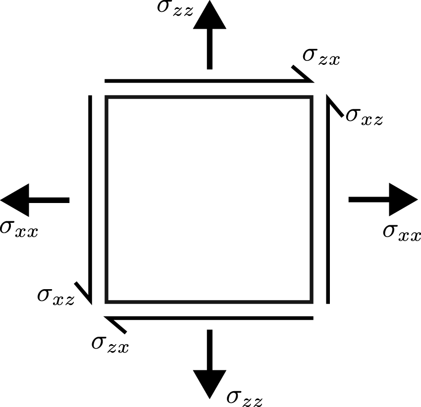

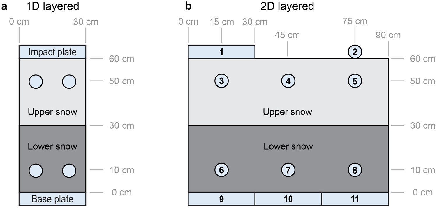
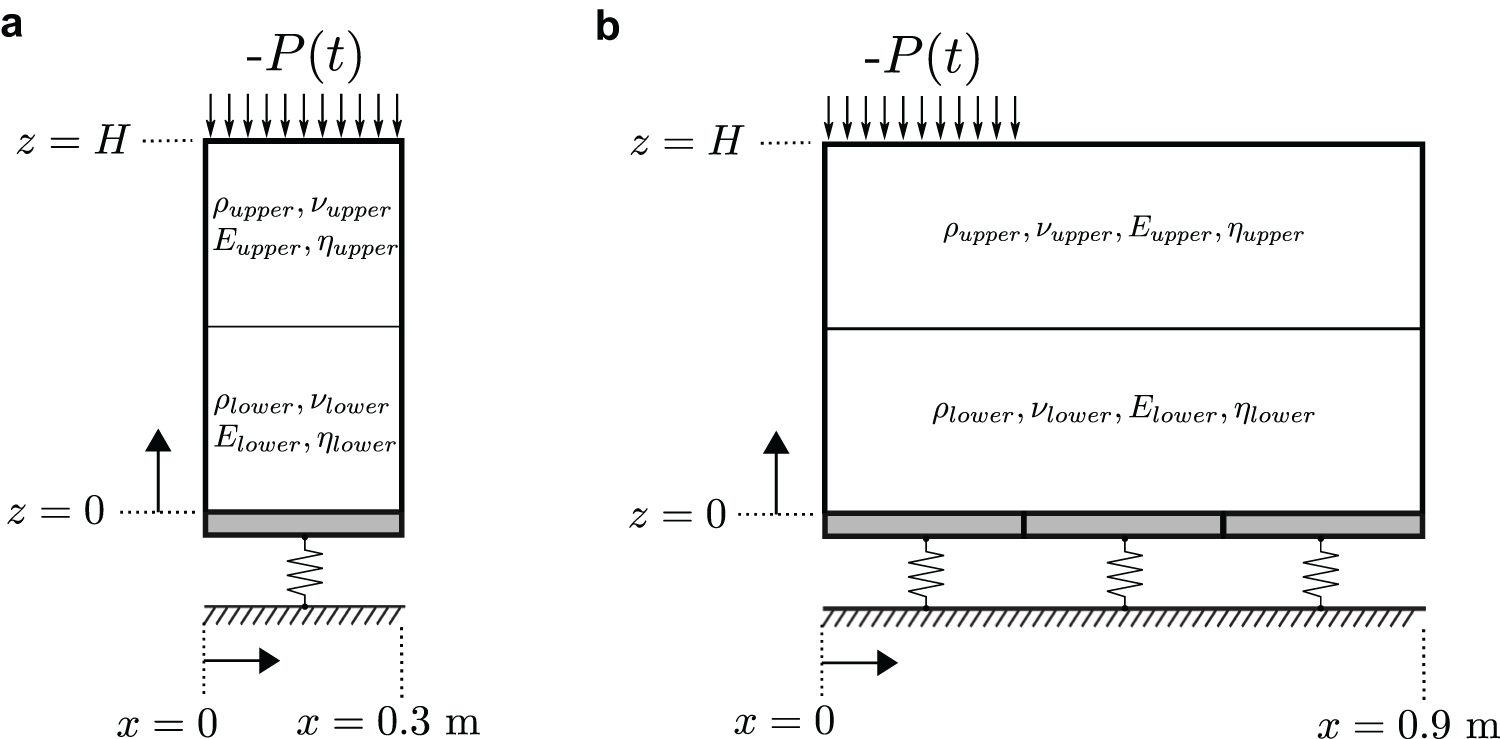


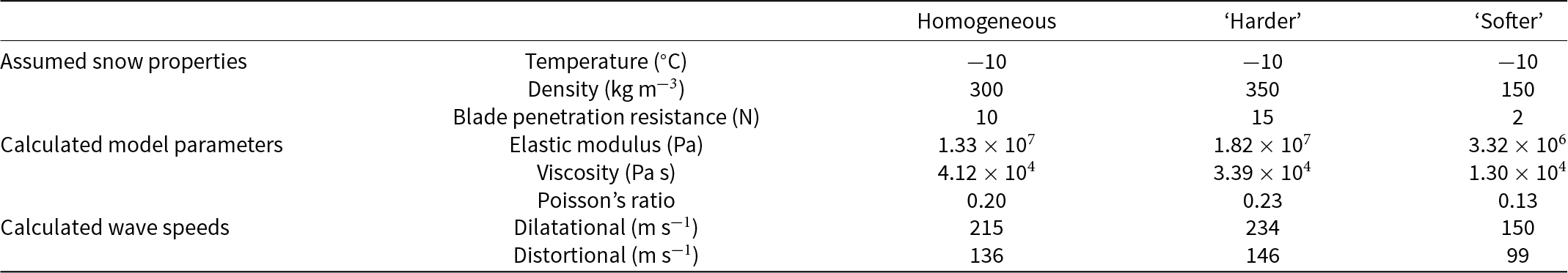


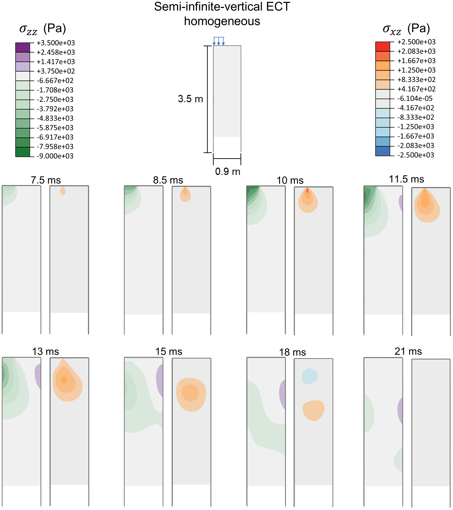


 Open access