


Introduction
Aedes aegypti is a mosquito of African origin that transmits several vector-borne illnesses of international concern, including dengue fever, Zika virus, yellow fever, and chikungunya. Aedes aegypti begins as an egg and matures through multiple aquatic life stages before reaching adulthood; at each stage, maturation and mortality rates are temperature dependent (Tun-Lin et al., Reference Tun-Lin, Burkot and Kay2000). In the absence of manmade infrastructure, the vector's survival is contingent on natural climate conditions. However, A. aegypti's preference for feeding on human hosts leads the vector to occupy regions populated by humans, where manmade infrastructure provides temperature and wetness conditions more conducive to survival than found in habitats lacking in manmade infrastructure (Ritchie et al., Reference Ritchie, Montgomery and Hoffman2013). Beyond understanding the geographical range in which A. aegypti can survive outdoors, analyzing the scope of its viability in areas with significant human populations can inform the knowledge of measures that prevent vector spread and disease transmission.
Habitat heterogeneity is a central factor in vector survival and an essential consideration for the development of control strategies. In cities and suburbs with ample manmade infrastructure, the vector migrates freely among outdoor habitats (natural or manmade, subject to outdoor temperature fluctuations, with humans assumed to be present), indoor habitats (with approximately constant temperature and humans present), and enclosed habitats (temperature moderated exterior spaces with no humans present, such as water tanks, water towers, and underground sewage systems) in search of feeding subjects and oviposition sites. While outdoor habitats are fully exposed to weather patterns, indoor habitats are climate-controlled, and enclosed habitats are somewhat sheltered from exterior conditions (Russell et al., Reference Russell, Kay and Shipton2001). In this study, a separate set of temperature conditions governs each of these habitat types and the balance among them is adjusted to explore the possibility of vector population reduction through habitat control.
This study integrates findings from multiple sources that describe common A. aegypti habitats. Barrera et al. studied pupal counts in Puerto Rico to determine the containers from which A. aegypti adults emerged. Using cluster analysis to show mosquito distribution, Barrera et al. concluded that the largest populations of pupae were found in outdoor habitats, specifically unattended, rain-filled containers in yards, suggesting that A. aegypti control is best achieved by managing these household containers (Barrera et al., Reference Barrera, Amador and Clark2006). Burke et al. affirm the viability of the vector in enclosed habitats. Burke et al. studied septic tanks to show the relationship between mosquito prevalence and the physical characteristics of a tank, such as surface area and cracks in the exterior. While Burke et al. concluded that the presence of resting mosquitos in a septic tank does not necessarily mean they developed there, their study of these tanks validates the consideration of enclosed habitats (Burke et al., Reference Burke, Barrera, Lewis, Kluchinsky and Claborn2010). Ritchie et al. and Troyo et al. studied urban habitats to estimate the total size of the adult A. aegypti population, as well as the areas mosquitos are most likely to inhabit. Ritchie et al. released a group of mosquitos in Queensland, Australia, and compared numbers of trapped mosquitos before and after release to estimate the size of the total mosquito population relative to the released population. In addition to deriving a population count, Ritchie et al. indicated that A. aegypti mosquitos are most prevalent in urban areas (Ritchie et al., Reference Ritchie, Montgomery and Hoffman2013). Similarly, Troyo et al. surveyed a region in Costa Rica and characterized habitats by setting, type, and capacity. Troyo et al. determined that over 80% of larval habitats were found in outdoor habitats on household lots, with domestic animal drinking containers, washtubs, and manholes among the most common (Troyo et al., Reference Troyo, Calderón-Arguedas, Fuller, Solano, Avendaño, Arheart, Chadee and Beier2008). These studies of A. aegypti breeding sites affirm the three broad habitat categories considered for vector development.
The model presented here expands upon preexisting studies of A. aegypti population dynamics by synthesizing previous research findings with specific characteristics of the regions and habitat types of interest. Some models include temperature-dependent maturation and death rates (Bar-Zeev, Reference Bar-Zeev1958, Dye Reference Dye1984, Focks et al., Reference Focks, Haile, Daniels and Mount1993, Magori et al., Reference Magori, Legros, Puente, Focks, Scott, Lloyd and Gold2009, Yang et al., Reference Yang, Macoris, Galvani, Andrighetti and Wanderley2009). This model extends them to include multiple lifecycle stages, wet and dry oviposition sites, multiple types of habitats with different temperature profiles, and migration between these habitats.
Given the persistent risk of vector survival and disease transmission in the United States, this study examines the A. aegypti population's response to annual temperature fluctuations in five cities: El Paso, TX, a region close to the initial arrival site of Zika virus and dengue fever, which remains at risk for A. aegypti breeding and dispersal; New York, NY; New Orleans, LA; Orlando, FL; and Miami, FL. Climate conditions in each of these regions, which range from humid continental with cold winters to subtropical with year-round warm temperatures, present distinct risk levels for disease transmission (Monaghan et al., Reference Monaghan, Morin, Steinhoff, Wilhelmi, Hayden, Quattrochi, Reiskind, Lloyd, Smith, Schmidt, Scalf and Ernst2016). In addition to comparing the simulation outcomes with observations across all five cities, the model for El Paso is considered in further depth by varying the availability of indoor, outdoor, and enclosed habitats.
This paper synthesizes information on maturation, survival, and oviposition into a novel lifecycle model that accounts for habitat heterogeneity and migration among habitats. A system of ordinary differential equations describing the A. aegypti lifecycle is proposed and constant and temperature-dependent maturation and mortality parameters are derived from the literature. The model is analyzed at equilibrium to identify a range of temperatures at which the vector population can viably reach a constant level. Numerical simulations describe the effects of habitat variability and regional weather patterns on vector prevalence. Model simulations for five cities are used to compare predicted mosquito abundance based on outdoor habitat only against a prior model described by Monaghan et al. (Reference Monaghan, Morin, Steinhoff, Wilhelmi, Hayden, Quattrochi, Reiskind, Lloyd, Smith, Schmidt, Scalf and Ernst2016). The example of El Paso is developed in more detail to illustrate the importance of alternative habitats to the pattern of mosquito abundance, in particular showing the persistence of populations even when no outdoor or indoor habitat is available. The habitat distribution producing the most adult mosquitoes is found for El Paso. This distribution is compared with the 100% outdoor habitat assumption present in prior models, for the four remaining cities.
Methods
A system of ordinary differential equations describes population dynamics within a single aquatic habitat for eight stages of the A. aegypti lifecycle: dry eggs, wet eggs, two larval groups, pupae, and three adult groups. The model accounts for mosquitos appearing in outdoor, indoor, and enclosed habitats. To represent the differences in maturation patterns that result from varying temperature and wetness in these spaces, three parallel versions of these differential equations are each controlled by temperature and wetness patterns specific to one type of habitat. Transitions within habitat types reflect maturation from one life stage to the next; transitions between habitat types represent physical migration. Figure 1 shows the interactions between components in the model.
Flow diagram for the vector lifecycle. Each box represents one of eight life stages in one of three habitats. Solid arrows represent biological transitions such as maturation, while dashed arrows represent flooding and migration. The model for each habitat type is described by the system of ordinary differential equations specified in equations 1–8.

Model equations
Within each of the three habitats, a system of ordinary differential equations represents fluctuations in the eight life stages. Terms in these equations align with the arrows showing transitions between life stages in fig. 1. Generally, the population in each stage increases as a result of maturation from the prior stage or migration from another habitat and decreases as a result of maturation into the next stage, migration out of the habitat, or death. Table 1 lists descriptions of the parameters and variables included in these eight equations, along with units and the sources from which they are derived. Temperature-dependent parameters, which include eggs laid per female per day (e b), larval and pupal maturation and death rates (n Ls, n Lb, n P, f s, f b, f P), and the length of the oviposition cycle (l v), are listed alongside the corresponding equations. All other parameters, including egg flooding, eclosion, and death rates (n Ed, n Ew, q Ed, q Ew), density-dependent larval death rates (q Ew, q Ed), the rate of adult transition into egg-laying (n a), and the daily adult death rate (d a), are listed with constant values.
Description of parameters and variables

Outdoor habitat modifications to include migration of adults
Migration rates of adult mosquitoes between habitats are controlled by the availability of wet oviposition sites or the availability of humans on which to feed. Feeding adults are assumed to migrate into the outdoor habitat from the indoor and enclosed habitats in search of humans to bite, and out of the outdoor habitat in search of blood meals in indoor spaces. Indoor habitats are defined as interior, temperature-moderated spaces, such as homes and buildings, that are not exposed to temperature variations. Two unique assumptions defining the enclosed habitat are that it is entirely wet and that it has no human subjects available for biting (Russell et al., Reference Russell, Kay and Shipton2001). These characteristics alter both the oviposition and migration patterns for adults in enclosed habitats.
Complete system of habitat-specific equations
Incorporating the modifications described above, the complete model consists of a system of 23 ordinary differential equations, which include eight equations each for the outdoor and indoor habitats and seven equations for the enclosed habitat. As these equations are similar in character to many models in the literature, the complete description of each of them is given in Appendix 1. The system of equations by habitat, including both biological and spatial transition terms, is as follows. Note that the factor of ½ in the coefficients of pupal terms representing transition to the adult stage represents the simplifying assumption that half are female.
Outdoor habitat model:


Indoor habitat model:


Enclosed habitat model:


Annual temperature models for El Paso, Miami, New Orleans, Orlando, and New York
Several of the maturation and death parameters in the above model depend upon temperature and the available habitat area. This section describes temperature models for the three habitats in the five U.S. cities of interest. This model only considers seasonal temperature patterns in order to establish annual insect trends. If the research question included the prediction of mosquito abundance at specific times it would be appropriate to include daily temperature variation either as direct data or with stochastic models, as is done in other models (Morin and Comrie, Reference Morin and Comrie2010; Morin and Comrie, Reference Morin and Comrie2013); Morin et al., Reference Morin, Monaghan, Hayden, Barrera and Ernst2015; Lega et al., Reference Lega, Brown and Barerra2017).
Outdoor temperature
A model derived from daily average temperature data from each city represents annual outdoor weather patterns (U.S. Climate Data). Temperatures in these cities range from annual lows of below 0 °C in early January to highs of over 30 °C in July and August, making the viability of mosquito survival highly variable. A truncated Fourier series is used to fit annual daily mean temperature data. Expressions for all five cities are in Table 1.
Indoor temperature
Because indoor spaces are climate-controlled, the indoor habitat is assumed to remain at a constant temperature year-round. Temperatures in the indoor habitat are defined at a constant 21 °C, representing the average indoor temperature of climate-controlled American households.
Enclosed temperature
The relationship between underground and surface temperatures provides a proxy for the insulating effect of enclosed habitats. In a study of underground wine storage areas, Tinti et al. report an external temperature amplitude of 15.5 °C and an underground temperature amplitude of 7.6 °C, implying that the ratio of underground to above-ground fluctuations is 0.49 (Tinti et al., Reference Tinti, Barbaresi, Benni, Torreggiani, Bruno and Tassinari2015). In addition to scaling the amplitude of the outdoor Fourier function by this value, a lag of two weeks between outdoor and enclosed temperatures is introduced. This modification is based upon the assumption that insulated spaces retain heat and cold for longer periods than exposed environments, as well as Naylor's finding that underground soil reached its annual peak temperature about 14 days after the soil surface in Indiana (Naylor and Gustin, Reference Naylor and Gustin2017). The resulting function determines the temperature of the enclosed habitat, given for all cities in Table 1. Figure 2 shows the resulting temperature patterns for all five cities.
A comparison of outdoor, indoor, and enclosed temperature models for all five cities. The blue (Outdoor) curve shows the best-fit Fourier series, the orange (Indoor) line shows constant temperature in climate-controlled spaces, and the yellow (Enclosed) curve is modified to represent a reduced amplitude and time lag for enclosed temperatures.

Lifecycle parameters
Temperature models for the three habitat types are used to calculate the maturation and death parameters for the system of differential equations described above. This section outlines the derivation of either a constant value or a temperature-dependent function for each population parameter in the model.
Egg production rates (eb, pwo, pwi)
Egg production is determined by the proportion of eggs laid in wet habitats (p w), the number of egg-laying adult females (A 2), and the number of eggs produced per female per day (e b). For the adults remaining in the indoor and outdoor habitats during oviposition, the proportion laying in aquatic habitat is taken to be very close to one unless there is no aquatic habitat available, using the Holling Type II functional response in Table 1. In enclosed areas, a 100% wet laying proportion is assumed.
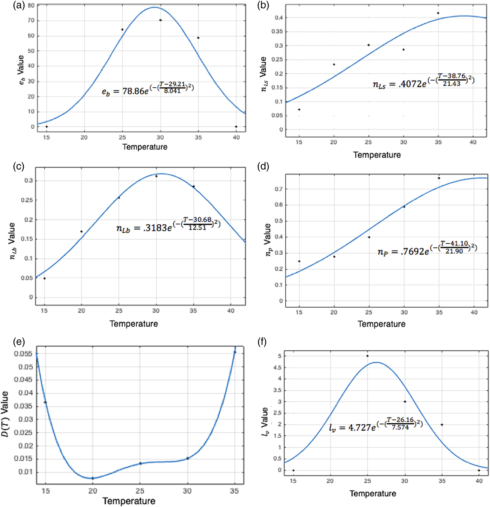
Costa et al. report the mean number of eggs laid daily per adult female under two humidity conditions at each of three temperatures (Costa et al., Reference Costa, Santos, Correia and Albuquerque2010). These results are averaged at 25, 30, and 35 °C and the number of eggs laid daily is set to zero at 10 and 40 °C given Yang observed that oviposition did not occur at or beyond these temperatures (Yang et al., Reference Yang, Macoris, Galvani, Andrighetti and Wanderley2009). A best-fit Gaussian function is fit to these data to describe the number of eggs laid per female per day by temperature, which is used to derive e b for each temperature and habitat, stated in Table 1. Values of this function are shown by temperature in fig. 3a.
Curve fitting sessions to determine the best-fit values for temperature-dependent equation parameters. The big larva maturation rate, oviposition cycle length, and eggs laid daily per female peak in the middle of the temperature range, between 25 and 30 °C. The remaining two maturation rates peak at warmer temperatures of around 35 °C. Death rates are lowest between 20 and 30 °C, indicating that moderate temperatures are most conducive to daily survival.
Egg flooding and eclosing rates (ned, new)
Oviposition occurs in either a wet or a dry area according to the proportion of adult females laying in wet habitats. While eggs can remain viable for several months under dry conditions, they must become submerged in order to eclose (Focks et al., Reference Focks, Haile, Daniels and Mount1993). Assuming that breeding takes place in primarily manmade containers, and that human activity is the main source of flooding, one might expect containers to be filled every other week through lawn watering, sprinklers, the filling of animal dishes, etc. both indoors and outdoors, giving a daily flooding rate (n Ed) of 0.071. There is no enclosed habitat flooding rate, as all eggs in this habitat are initially laid in wet areas.
For eggs laid in wet areas, and for originally dry eggs that have become submerged, transition out of the egg stage is determined by the eclosion rate (n Ew). Focks et al. report a daily mean eclosion rate of 59.6% among wet eggs when submerged in water above 22 °C; however, they acknowledge that this threshold may be too high (Christophers, Reference Christophers1960, Focks et al., Reference Focks, Haile, Daniels and Mount1993). As eclosion rates are relatively fast, the assumption was made that the transition from wet to dry is negligible and is omitted in the model.
Egg death rates (qEd, qEw)
Faull and Williams report the mean survival time of A. aegypti eggs at varying levels of warmth and dryness to show the ongoing survival and viability of eggs laid in dry locations. On average, the eggs could survive 187.4 days under dry conditions and 229.3 days under wet conditions (Faull and Williams, Reference Faull and Williams2015), inverted to give death rates of 0.0053 (q Ed) and 0.0044 (q Ew) for dry and wet eggs, respectively.
Maturation rates for larvae and pupae (nLs, nLb, nP)
In the larval and pupal stages, maturation parameters are temperature-dependent. Tun-Lin et al. studied maturation times and survival rates at five temperatures, ranging from 15 to 35 °C, and found that the time to maturation decreased consistently as temperatures rose within this range, consistent with other studies (Sharpe and DeMichele, Reference Sharpe and DeMichele1977, Rueda et al., Reference Rueda, Patel, Axtell and Stinner1990, Tun-Lin et al., Reference Tun-Lin, Burkot and Kay2000). A Gaussian curve is fit to Tun-Lin et al. in order to describe temperature-dependent maturation rates for each stage. Parameter values for the best-fit equation at each stage are recorded in Table 1 and shown in fig. 3b, d.
Temperature-dependent death rates for larvae and pupae (fs, fb, fP)
Tun-Lin et al.'s observed survival rates and maturation times at each of five temperatures lead to survival half-lives, giving death rates for each temperature. A polynomial is fit to these death rates, given in Table 1. Figure 3e affirms that the values of D as determined by this polynomial remain greater than zero both within and beyond the temperature range included in Tun-Lin et al.'s study (Tun-Lin et al., Reference Tun-Lin, Burkot and Kay2000).
Death rate for pupae, density-dependent death rates for larvae (qLs, qLb)
Studies by Barbosa et al. and Moore et al. affirm the importance of density-dependent development parameters. Barbosa et al. observed eggs at eight different density levels and determined that high-density groups had higher mortality rates as a result of lessened food availability. Barbosa et al. found that crowding had a non-linear effect on survival rates, affirming the adoption of quadratic density-dependent death rates from the Anopheles gambiae model (Barbosa et al., Reference Barbosa, Peters and Greenough1972, Wallace et al., Reference Wallace, Prosper, Savos, Dunham, Chipman, Shi, Ndenga and Githeko2017). In another study of larval density, Moore et al. observed the production of growth retardant factors (GRF) in a colony in Puerto Rico. Moore et al. concluded that nutrition, not density, influences the production of GRF, implying that the density-dependent factors for which the model accounts are primarily physical rather than chemical (Moore and Whitacre, Reference Moore and Whitacre1972). Based on findings from these studies, this model considers the density-dependent death rate as a grouping of the combined effects of predation and crowding.
Southwood et al. observed mean daily adult emergence rates, as well as counts of eggs, larvae, and pupae appearing in manmade containers. Water jars were the primary breeding areas for mosquitos, with an average of 54.84 adults emerging daily from 100 jars (Southwood et al., Reference Southwood, Murdie, Yasuno, Tonn and Reader1972). The estimated surface area of 1 m2 for the average water jar in Thailand is used to calculate a daily mean emergence rate of 0.5484 adults per m2 of water available for breeding (Visvanathan et al., Reference Visvanathan, Vigneswaran and Kandasamy2015). This rate corresponds to n pP in equation 6 of the model.
The remaining equations are solved at equilibrium at a constant temperature of 21 °C, which is the defined indoor temperature and falls within the range of outdoor temperatures in all cities. Southwood et al.'s emergence rate provides a constant value for P at this temperature. Southwood et al. report larval counts over the course of one year in water jars, and these values are averaged to derive a ratio of small to big larvae of 389/190. Based on these, algebraic manipulations of the equations for pupae and larvae lead to the value for q Lb reported in Table 1. The same calculations for large and small larvae at equilibrium yield the value of q Ls based on the ratio of wet eggs to small larvae. Using these values for q Ls and q Lb, the model reproduces the instar ratios from Southwood et al.'s field study when the system is solved at equilibrium.
Adult transition and death rates (n a, d a, l v)
The pupal maturation rate (n P) determines the rate of entry into the feeding adult stage. This value is halved to include only adult females, the only group that feeds and reproduces, assuming a 1:1 sex ratio (Sheppard et al., Reference Sheppard, McDonald, Tonn and Grab1969). In addition to maturing from the aquatic stages into a first feeding cycle, vectors re-enter the feeding adult stage between reproductive periods to begin a second cycle (Judson, Reference Judson1967).
The feeding population decreases in part as a result of transition into the egg-laying stage. Based on Costa et al.'s observation that mosquitos did not lay eggs within the first three days of reaching adulthood under any temperature conditions, the rate of maturation out of the feeding stage (n a) is taken to be 1/3 (Costa et al., Reference Costa, Santos, Correia and Albuquerque2010). The daily adult death rate (d a) of 0.11 corresponds to a mean daily adult survival rate of 89% (McDonald, Reference McDonald1977).
Adults transition into the egg-laying stage from the feeding stage, and the egg-laying population decreases as a result of the end of each oviposition cycle and death. The length of an oviposition cycle is temperature-dependent (Costa et al., Reference Costa, Santos, Correia and Albuquerque2010). A Gaussian function, lv, is fit to Costa et al.'s oviposition cycle data to describe the length of the egg-laying period by temperature, recorded in Table 1. Values are shown in fig. 3f.
At each temperature, the rate at which adults exit the egg-laying stage – either to begin another feeding period or to complete the final oviposition cycle – is taken as the inverse of this value (1/l v). The death rates of egg-laying and post-egg-laying adults take on the same constant value as the death rate of feeding adults (d a).
Migration rates (moi, mio, meo, m2io, m2oi, m2oe)
Because of the limited availability of data describing mosquito migration patterns among habitats, estimated migration rates are based on the vector's needs in each stage of the gonotrophic cycle. Migration rates in the feeding stage are determined by the availability of humans to bite. It is assumed that all feeding mosquitos in the enclosed habitat migrate to the outdoor habitat (m eo = 1) in order to feed. Migration rates between the indoor and outdoor habitats are estimated based on human activity. Given that the average person spends about two hours outdoors per day, and under the simplifying assumption that this time is evenly distributed, it is assumed that 8.3% of humans are outdoors and 91.7% are indoors at any given time (Diffey, Reference Diffey2011). These values are divided by three days, the average length of the feeding period, to derive daily outdoor-to-indoor and indoor-to-outdoor feeding migration rates (m oi, m io).
During the egg-laying stage, migration among habitats is treated as a function of the available wet oviposition area. The constants k o, k i, and k e represent the areas of outdoor, indoor, and enclosed aquatic habitat, respectively, resulting in a total wet laying area of k tot = k o + k i + k e. In a study of oviposition preferences, Edman et al. found that only 5.8% of initially gravid A. aegypti mosquitos were recaptured in their original locations when left to lay in entirely dry environments (Edman et al., Reference Edman JD, Scott, Costero, Morrison, Harrington and Clark1998). This finding suggests a high rate of departure from each habitat in the absence of wet laying area, which is incorporated into the migration rates.
Edman et al. indicate that α = 94.2% of adults leave each habitat during the oviposition period in the complete absence of wet laying area (Edman et al., Reference Edman JD, Scott, Costero, Morrison, Harrington and Clark1998). For indoor to outdoor migration, this value is multiplied by (k o/(k o + k i)), the proportion of the combined indoor and outdoor habitats made up by the outdoor habitat. This rate is divided by lv, the length of the oviposition period, to represent daily migration.
The remaining two oviposition migration rates describe migration from the outdoor habitat to indoor and enclosed areas. For each of these rates, α is multiplied by (1 − (k o/k tot)), yielding a rate that is inversely related to the proportion of the total wet laying area that the outdoor aquatic habitat comprises. The outdoor-to-indoor and outdoor-to-enclosed rates are multiplied by (k i/(k i + k e)) and (k e/(k i + k e)), respectively. These equations are summarized in Table 1.
Numerical simulations
Risk maps for A. aegypti are usually based on outdoor temperatures, which govern population dynamics in outdoor habitats. The first numerical experiment simulates one year of population fluctuations in each region given a constant outdoor wet habitat area of 1 m2 and no indoor or enclosed habitat, with migration rates set to zero, ensuring that the population exists entirely outdoors. Figure 4 shows the resulting population levels for these five initial simulations (fig. 4a–e) as well as the five annual temperature patterns (fig. 4f) and an example of larvae and egg populations for El Paso and New York (fig. 4g, h). The plot for each city shows fluctuations in its outdoor adult population over one year after reaching a periodic solution.
(a–f) Outdoor population levels by U.S. city in the absence of migration. Each simulation shows population dynamics over one year for 1 m2 of exclusively outdoor aquatic habitat governed by the climate model corresponding to the designated city. All migration rates during feeding and laying are set to zero to remove the possibility of departure to other habitats. (a) El Paso, TX; (b) New York, NY; (c) New Orleans, LA; (d) Orlando, FL; (e) Miami, FL; (f) Average monthly temperatures over one year for five U.S. cities. (g, h) Outdoor population levels for dry eggs, wet eggs, and small larvae in the absence of migration. Each simulation shows population dynamics over one year for 1 m2 of exclusively outdoor aquatic habitat governed by the climate model corresponding to the designated city. All migration rates during feeding and laying are set to zero to remove the possibility of departure to other habitats. Results are shown for (g) El Paso, TX and (h) New York, NY.

A second set of simulations tests a range of habitat allocation patterns under El Paso temperatures. Indoor and outdoor habitat allocations vary by 20% increments with the balance made up by enclosed habitat. Migration is allowed between habitats. Figure 5 shows the resulting time series for four choices of habitat allocation. Figure 6 shows the results of all parameter sets for maximum, minimum, and total annual adult mosquito populations as a series of heat maps.
Daily adult population by habitat distribution in El Paso, TX with migration. In each simulation, the blue curve represents the daily outdoor adult population, the orange represents the daily indoor adult population, the yellow represents the daily enclosed adult population, and the black represents the total daily adult population. Aquatic area is restricted to 1 m2 and appears in the following proportions: (a) 100% outdoor habitat, (b) 100% indoor habitat, (c) 100% enclosed habitat, (d) 30% outdoor, 30% indoor, 40% enclosed habitat.

Annual maximum, minimum, and total adult populations by habitat balance in El Paso, TX, with migration. In each heat map, outdoor, indoor, and enclosed areas are varied by increments of 0.2 m2 to maintain a constant total area of 1 m2. (a) The first map shows the highest population level reached annually and (b) the second shows the lowest, calculated as the maximum and minimum values of the solution curve, respectively, once periodicity is reached. (c) Total annual adult population by habitat balance in El Paso, TX. Population levels are determined given the same habitat distribution patterns as in Figures 6ab. In each case, the total annual adult population is calculated as the sum of the area under the solution curve over 365 days once periodicity is reached. (d) Daily adult population in El Paso, TX with habitat types balanced to maximize annual population totals. Habitat distribution is set to 1 m2 appearing 80% outdoors and 20% indoors. Outdoor, indoor, enclosed, and total solution curves appear in the same colors as in previous simulations.

A third set of simulations analyzes the impact of indoor habitat availability in three regions to understand how the redistribution of habitat into climate-controlled spaces changes the size of the adult population in each climate. New York, New Orleans, and Miami are the three sample cities selected for this simulation. In New York, temperatures fall below 21 °C for much of the year, and indoor habitats are expected to present more optimal temperature conditions than outdoor in the winter. New Orleans offers warmer outdoor conditions, with temperatures falling above and below 21 °C for roughly equivalent portions of the year. Finally, in Miami, where outdoor temperatures are almost always greater than indoor, migrating indoors to feed or lay may not have a positive effect on the vector population. Five-year simulations with migration are shown for each of these three temperature profiles. A total habitat area of 1 m2 is maintained, with a balance of 0.8 m2 outdoor, 0.2 m2 indoor, and no enclosed habitat, to follow the optimal distribution derived for El Paso in the first simulation. The same simulations with migration are also shown for 1 m2 of outdoor habitat. Figure 7 includes all outdoor, indoor, enclosed, and total populations for all six runs.
Impact of indoor habitat re-introduction, with migration, in (a) New York, NY, (c) New Orleans, LA, and (e) Miami, FL, three cities with varying levels of annual vector viability. Outdoor, indoor, enclosed, and total populations are plotted over five years with the optimal El Paso habitat balance of 0.8 m2 outdoor habitat and 0.2 m2 indoor habitat. For comparison, populations are shown for 100% outdoor habitat with migration, in (b) New York NY, (d) New Orleans, LA, and (f) Miami, FL.

Finally, a fourth set of simulations demonstrates the effect of enclosed habitat on vector survival. A total habitat area of 1 m2 is maintained, with 100% of the available habitat appearing in enclosed spaces. Results for El Paso are shown with the complete set of habitat simulations for that region in fig. 5, and results for the remaining four cities are shown in fig. 8.
Population dynamics in (a) New York, NY, (a) New Orleans, LA, (c) Orlando, FL, and (d) Miami, FL with 100% enclosed aquatic habitat and migration. Outdoor, indoor, enclosed, and total populations are plotted over five years and appear in the same colors as in previous simulations.

All simulations were done using Matlab software and the ODE45 solver (Mathworks).
Model analysis and equilibrium viability
While temperature fluctuations cause changes to the vector population in most habitats, it is possible for the population to reach equilibrium at a constant temperature. We make use of the following theorem to confirm temperature ranges for viable populations.
Theorem 1
Consider the following function of the model parameters:
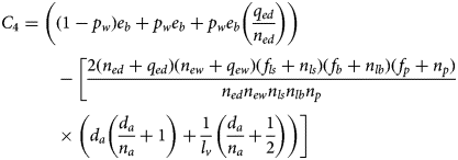
For an equilibrium to exist with all populations positive, it is necessary and sufficient that C 4 be positive. The proof of this theorem is in Appendix 2.
The parameters comprising C 4 offer a biological interpretation of the necessary conditions for equilibrium viability. The first term is an egg production rate, expressed as the sum of the number of wet and dry eggs laid per adult per day and the ratio of the dry egg death to flooding rates. The second is a ratio of the products of the rates of exit, via maturation and death, to the rates of entry, via maturation, for each stage. A large value for this term (yielding a negative value for C 4) indicates that death rates far exceed maturation rates, leading to population decline. Conversely, equilibrium becomes viable when enough eggs are produced daily to compensate for the rate of death or maturation out of each of the subsequent life stages.
The temperature-dependent formulas for maturation and death rates are used to solve for the zeroes that result when C 4 is evaluated as a function of temperature. Figure 9a shows the sign of this coefficient over a temperature range of 15 to 40 °C. The coefficient changes sign at 16.16 and 38.32 °C, indicating that the population cannot reach equilibrium, even under constant temperature conditions, when the temperature is outside of this range.
(a) Theorem 1 yields an expression, C4, whose sign determines the viability of mosquito populations for given model parameters. The value of this expression, shown here, varies with temperature. The solid line shows the value of the C4 by temperature from 15 to 40 °C, while the dashed line shows the temperature values at which the coefficient passes zero. The graph affirms that the coefficient C4 changes sign at 16.16 and 38.32 °C. (b) Equilibrium adult population by temperature. At each temperature within the range of equilibrium viability, the adult population is calculated at a constant temperature over an adequate period to reach equilibrium. The Matlab plotting tool is used to determine each resulting constant adult population and plot these values as a function of temperature.

While the populations in all eight life stages reach constant levels at any temperature within the range shown in fig. 9a, the size of the equilibrium population varies with temperature. Matlab's ODE45 solver is used to compute the size of the total daily adult population, A 1 + A 2 + A 3, that is present at equilibrium given constant temperature conditions at each level from 17 to 38 °C. This value is close to zero on the low end of the temperature spectrum, and it increases non-linearly until reaching a maximum at 30 °C, where 28.56 total adults are present daily per square meter of aquatic habitat. Beyond 30 °C, the equilibrium adult population level falls rapidly before again becoming negligible at the warmest temperatures. Results are shown in fig. 9b.
Results
The five cities modeled in this study are reported to have some level of persistent vector risk and simulations are expected to show consistent survival rates and high summer population levels (Monaghan et al., Reference Monaghan, Morin, Steinhoff, Wilhelmi, Hayden, Quattrochi, Reiskind, Lloyd, Smith, Schmidt, Scalf and Ernst2016). Monaghan et al. show the range of A. aegypti in the United States and establish risk levels based on the Skeeter Buster model (Monaghan et al., Reference Monaghan, Morin, Steinhoff, Wilhelmi, Hayden, Quattrochi, Reiskind, Lloyd, Smith, Schmidt, Scalf and Ernst2016). For that experiment, a city is selected from each reported level of vector prevalence risk and results are compared to predicted population levels in each region. Table 2 lists Monaghan et al.'s qualitative reports of the vector prevalence risk in each city. Figure 4f shows average temperatures over one year in each of the five cities. Note that the inclusion of indoor and enclosed habitats in the model given here is a novel addition that distinguishes it from the models such as Skeeter Buster that are typically used to produce risk maps.
Average temperatures and reported vector prevalence in five U.S. cities (from Monaghan et al., Reference Monaghan, Morin, Steinhoff, Wilhelmi, Hayden, Quattrochi, Reiskind, Lloyd, Smith, Schmidt, Scalf and Ernst2016).

Outdoor habitat dynamics
The range of equilibrium viability aligns closely with the risk levels reported by Monaghan et al. In New York, El Paso, and New Orleans, where winter temperatures fall below the lower viable bound for several months of the year, Monaghan et al. report no risk of vector prevalence in January. In Orlando, where the lowest temperature falls on the border of the viable range, winter vector prevalence is low. In Miami, temperatures always remain within the optimal range for vector survival, and a moderate to high year-round population is anticipated.
Outdoor habitat simulations for each of the five cities, as shown in fig. 4a–e, match expectations drawn from Monaghan et al.'s study. In peak vector season, there is little distinction among New Orleans, Orlando, and Miami, which are designated as high-risk; all three cities support peak daily populations of just under 30 adults per square meter of aquatic habitat. Peak population levels for New York and El Paso are less aligned with Monaghan et al.'s study, which indicates a larger presence of A. aegypti adults in New York than in El Paso. However, the relative maximum population levels of the two cities are reasonable given that both summer and winter temperatures are warmer in El Paso than in New York.
At colder temperatures, differences in risk levels among regions are also clear. El Paso, New York, and New Orleans have negligible adult populations between January and April, true to the reported non-existent risk level and the relatively long periods during which the temperatures of all three regions fall below the lower bound of equilibrium viability. In Orlando, the population falls just above the threshold for a year-round vector presence. Finally, as predicted, A. aegypti adults are present in Miami during even the coldest months of the year.
Optimizing habitat distribution
Vector population levels vary under El Paso temperatures depending on the predominant aquatic habitat type. When the available wet habitat is exclusively outdoors, the population peaks each summer, and more adults inhabit the outdoor habitat than any other. The total annual adult population, measured across all three habitats, is 2600 mosquitos per m2 aquatic habitat, reflecting the vector's ability to survive well under warmer conditions despite population drops in the winter of each year. Conversely, when the available habitat is entirely indoors, the vector survives year-round, but maintains a lower total population. In line with the equilibrium population level for 21 °C shown in fig. 9a, there is a constant daily population of about five adults, and the total annual population is around 2000 per m2 aquatic habitat. The case in which aquatic habitat exists only in enclosed spaces is least optimal for vector survival, and the total annual population only reaches about 300 adults per m2 aquatic habitat.
The minimum and maximum daily population levels by habitat allocation, summarized in fig. 6a, b, are consistent with these findings. While the maximum annual population is highest when the available habitat is entirely outdoors, winter population levels are negligible in the absence of indoor habitat. Annual population totals affirm the trade-offs between habitat ratios that maximize population levels and those that optimize year-round survival potential. The maximum total population appears when the square meter of available habitat includes 80% outdoor area, 20% indoor area, and no enclosed area. Population levels decrease along each subsequent diagonal, indicating that emergence rates become lower with increasing percentage of enclosed habitats.
The effect of a large percent of habitat being enclosed reflects the inefficiency of breeding in an environment in which there are no human subjects for feeding. Regardless of the level of enclosed habitat, however, peak total populations tend to appear along the 20% indoor habitat level. As fig. 6d shows, re-introducing 20% indoor habitat to the outdoor model allows the vector to survive indoors at a low level year-round without drastically reducing the annual peak populations. This adjustment produces the optimal balance among those explored for maximizing both population levels and survival potential.
Role of indoor habitat
The redistribution of outdoor habitat to indoor spaces produces varying effects across climates. In the simulation for New York, adult populations disappear in the winter, reappearing in warmer weather as seen in fig. 4h. Introducing a small portion of indoor aquatic habitat leads to a 50% increase in the total annual adult population compared to the entirely outdoor case, as summarized in fig. 7a, b and Table 3. Although the population still effectively disappears each winter, the presence of indoor breeding area increases both the length of time that the vector is present and the total number of adults that the habitat can support.
Annual adult populations with indoor habitat re-introduction in three selected cities
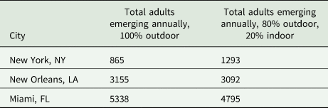
In New Orleans, as shown in fig. 7c, d, incorporating indoor aquatic habitat has little effect on the total annual adult population. When 20% of the aquatic habitat is redistributed to indoor spaces, the vector population remains viable at a very low level year-round and summer peaks are reduced. In contrast to the maximum population of about 25 adults per square meter that emerges in the entirely outdoor case, the New Orleans climate supports a peak of about 7 adults indoors and 12 outdoors per square meter of total aquatic habitat. The longer period of survival and larger winter population in both habitats compensate for these lower peaks in the total population counts.
Unlike in colder climates, reallocating a portion of the available habitat to indoor areas under Miami temperatures does not improve conditions for the vector population. Figure 7e, f demonstrate that A. aegypti adults survive year-round in Miami in the 20% indoor habitat case, but the summer peak levels and the total annual population are reduced. This outcome reflects the equilibrium population levels by temperature from the model. Given that Miami outdoor temperatures remain above the indoor level of 21 °C for all months except January, outdoor climate conditions are more favorable to the vector population than indoor spaces for most of the year.
Role of enclosed habitat
Population levels in the presence of 100% enclosed aquatic habitat are consistent with regional variations in temperature and outdoor population levels. In New York, where cold winter temperatures make the climate least conducive to outdoor vector survival, the population does not survive in exclusively enclosed habitat, as seen in fig. 8a. In New Orleans, the population fares better, with similar summer peaks and winter lows to the entirely enclosed population levels in El Paso.
As expected from their favorable year-round temperatures, Orlando and Miami support a nonzero vector population year-round even when aquatic habitat is entirely enclosed. In both cities, the outdoor, indoor, and enclosed populations remain roughly equivalent throughout each year, each reaching an annual maximum of slightly fewer than five adults and a minimum slightly above zero. In line with its warmer climate, Miami has the highest population levels of any of the five cities in this simulation. However, population totals remain significantly lower than with more optimal habitat balances (such as 100% outdoor habitat for Miami), affirming the difficulty of population growth in the enclosed habitat.
Discussion
The model developed here describes temperature-dependent fluctuations in the population of A. aegypti and evaluates the vector's growth and survival under three habitat conditions. The model is based on a range of estimates and several assumptions that could be sources of error, and results agree with some, but not all, prior studies. The results illustrate how this insect's adaptive survival mechanisms allow it to persist in a wide range of habitats, with temporal and spatial distributions that have implications for both vector and disease control. In particular, the analysis of outdoor habitats alone shows agreement with other models in the literature. The analysis of El Paso shows that mosquito populations can survive even without indoor or outdoor habits and that there is an optimal combination for mosquito abundance. The analysis of other cities shows the dependence of this observation on the local temperature profile.
Model performance
The conclusion that equilibrium is viable between approximately 16 and 38 °C informs subsequent evaluations of the survival potential of A. aegypti adults in the U.S. While most resulting findings on the vector's range and population levels are validated against preexisting reports, results diverge from the literature in a few areas. The Skeeter Buster model predicts higher vector risk in New York than in El Paso and shows no survival viability beyond a narrow swath of the southern and eastern United States (Monaghan et al., Reference Monaghan, Morin, Steinhoff, Wilhelmi, Hayden, Quattrochi, Reiskind, Lloyd, Smith, Schmidt, Scalf and Ernst2016). The model presented here suggests that the climate of southern Texas supports both a longer annual period of A. aegypti survival and higher population peaks than that of New York City. With the incorporation of indoor and enclosed habitats, this model tends to show a broader range of viability than has previously been modeled or observed in the United States.
Sources of error
Various sources of error influence these results. Temperature models are calculated from monthly average data rather than daily temperatures, which may have an effect. The vector lifecycle modeled does not account for every possible factor influencing population dynamics. In particular, temperature likely influences more death rates than those considered. In the larval stages, the density-dependent death rates are calculated based on average field counts and emergence rates over the course of a year (Southwood et al., Reference Southwood, Murdie, Yasuno, Tonn and Reader1972). These estimates are also imprecise given the age of Southwood et al.'s study and the use of annual averages to determine instar ratios. The assumptions made regarding the length of feeding and number of oviposition cycles are not likely to strictly hold under extreme temperature conditions. Additionally, the assignment of a constant daily adult death rate, rather than temperature-dependent adult mortality, may lead to an overestimation of the adult population under particularly inhospitable climate conditions. Finally, there are points of uncertainty in the definition of habitat types and migration patterns. Accounting for differences between shaded and exposed outdoor areas, buildings maintained at different or non-constant temperatures, and enclosed spaces varying from sewers to water towers would require a more detailed set of temperature equations for each habitat and provide more insight into the effects of habitat heterogeneity. While this model does not account for variations in wetness that arise in regions that are rainier than El Paso, an ideal study would more explicitly consider weather effects in the assignment of flooding rates.
Mechanisms of survival
The inclusion of multiple habitat types illustrates how the mechanisms of A. aegypti survival work in different climate conditions. In areas with winter temperatures low enough to kill off adult mosquitoes, the ability of dry eggs to survive in low temperatures allows outdoor populations to survive. In areas where there are enclosed subterranean habitats and where indoor populations are not yet established, mosquitoes that would not otherwise survive due to the drying up of outdoor habitats can survive. In climate-controlled indoor habitats, mosquito populations can become established anywhere.
Optimal conditions for population growth
The optimal distribution of habitat types at steady state varies from location to location. In El Paso, a small percent of indoor habitat increases the total annual population (figs. 5 and 6), whereas outdoor habitat is so productive in Miami that allocating a percent of aquatic habitat to indoor conditions will reduce the overall population (fig. 7). In New York, the presence of indoor habitats extends the season for adult populations (fig. 7).
In this model, a functional ‘choice’ of habitat is controlled by the availability of habitat, not any innate mosquito preference, although there may be some innate preferences for oviposition. For the example of El Paso, the percent of habitats in each category is varied, with the result shown in the heat maps of fig. 6, describing various outcomes resulting from mosquito habitat allocation, which controls the behavior of mosquitoes in the simulations.
Vector and disease control
This study shows that outdoor temperature alone is insufficient to predict populations. It is clear that all three types of habitat are important and should be monitored. Householders can be made aware of indoor and outdoor habitats on their property and can remove these. Subterranean enclosed habitats such as sewers or pipe leaks may also be sources of persistent mosquito populations and monitoring these is more likely to fall under the supervision of authorities. Detection and mitigation of such habitats should be a community-wide concern.
Future work
Two important directions of research emerge from this study. One concerns the role of flooding of eggs in population dynamics. Once eggs are flooded, maturation begins. Increased flooding could therefore increase the adult population by hastening this process, or it could diminish the adult population by beginning the maturation process under conditions of low temperature, causing eggs and larvae to die before completing maturation. Further work is needed to sort out the effects of flooding in colder regions.
Second, some habitat distributions favor overall mosquito abundance while others favor winter prevalence, leading to the question of which is worse for disease transmission. A full model with disease dynamics included is necessary to shed light on this question and many others arising from epidemiological concerns.
Summary
The model proposed in this study provides a foundation for understanding A. aegypti maturation, survival, and migration in urban and suburban areas within and beyond the United States. While estimating the size of the adult A. aegypti population is only a small step in guiding disease control, pairing this system of equations with a future disease dynamics model will hopefully capture the relationship between population levels and transmission rates more closely. Until then, this model offers a basis for evaluating the vector's range of viability and implies promising opportunities for vector control through habitat identification.
Appendix 1: Model Development
The rate of change of the dry egg population is expressed as the laying rate of eggs in dry places – the proportion of eggs laid in dry habitats (1 − p w) times the number of eggs laid daily per female (e b) times the number of egg-laying adult females (A 2) – less transition into the wet egg stage via flooding (n Ed) and death (q Ed).

The rate of change of the wet egg population is expressed as the sum of the laying rate of eggs in wet places (p wE bA 2) and the flooding rate of dry eggs (n Ed), less eclosion (n Ew) and death (q Ew).

The rates of change of the small and big larval populations are expressed as the eclosion rate of wet eggs (n Ew) and the maturation rate of small larvae (n Ls), respectively, less maturation into the subsequent stage (n Ls, n Lb), a linear temperature-independent death rate (f s, f b), and a quadratic density-dependent death rate (q Ls, q Lb).


The rate of change of the pupal population is expressed as maturation from big larvae (n Lb), less maturation into the first adult stage (n P) and death (f P).

Within the adult stages, population levels are determined by migration among habitats in addition to maturation and death. This overview discusses only the maturation and death factors that are common to all three habitats; migration terms will be incorporated in the following habitat subsections. The rate of change of the feeding adult population is expressed as the maturation of females from the pupa stage (n P) less transition into egg-laying (n a) and death (d a). An additional term represents the rate of return from the egg-laying stage to enter an additional oviposition cycle, which is expressed as the fraction of adults returning to complete another oviposition cycle, times the inverse of the length of an oviposition cycle (1/l v), times the number of egg-laying adults (A 2). Because adults complete two egg-laying cycles in their lifetime, the fraction returning to complete a second cycle is assumed to be ½ (Judson, Reference Judson1967).

The rate of change of the feeding adult population is expressed as transition into egg-laying (n a), less death (d a) and the rate of transition out of egg-laying (1/l v), which is the inverse of the length of an oviposition cycle.

A third adult stage is included to represent the population of adult females that have exited the egg-laying stage for the final time. The rate of change of this population is expressed as the exit rate from the final oviposition cycle (1/2 × 1/l v), less death (d a). For the purposes of model dynamics this stage is an output variable and may be ignored.

The rate of change of the outdoor feeding adult population is determined as in equation 6, with three added migration terms. Migration during the outdoor feeding adult stage is expressed as the sum of the rates of migration from enclosed and indoor spaces (m eo, m io), less the outdoor-to-indoor migration rate (m oi). Equation 6 is modified as:

The rate of change of the outdoor egg-laying population is determined as in equation 7, with three added migration terms. Both outdoor-to-indoor and indoor-to-outdoor migration are included. Departure from outdoor to enclosed habitats (m 2oe) is also included, but it is assumed that no laying adults migrate outdoors from enclosed habitats, as these habitats are entirely wet and are thus optimal for oviposition. Migration during the outdoor A 2 stage is expressed as follows. Note that migration rates during oviposition depend on habitat availability. Equation 7 is modified as:

Two migration terms describe the rate of indoor feeding population increase as a result of the arrival of mosquitos from outdoors (m oi), and the rate of decrease as a result of departure to outdoor habitats (m io). Equation 6 is modified as:

The rate of change of the indoor egg-laying population is determined as in equation 7, with two added migration terms. As the size of indoor and outdoor aquatic habitats fluctuates due to the filling and emptying of manmade containers, the vector is assumed to migrate to seek optimal oviposition sites. Migration terms in each direction (m 2oi, m 2io) are included. Equation 7 is modified as:

Equation 1, which describes the rate of change of the dry egg population, is not relevant to the enclosed habitat. Equation 2 describes the rate of change of the total enclosed egg population as listed above. The proportion of eggs laid in aquatic habitat (p w) is assumed to be 1, and no dry egg flooding rate is included.

The rates of change of the subsequent enclosed aquatic populations are determined as in equations 3–5.
The rate of change of the enclosed feeding adult population is determined as in equation 6, with one added migration term. No feeding adults are assumed to migrate into the enclosed habitat due to the lack of human inhabitants. Conversely, all enclosed feeding adults migrate outdoors to find blood meals. Migration at this stage thus includes only departure to the outdoor habitat (m eo). No maturation term from the enclosed feeding to egg-laying stage is included, as this transition is not possible without first migrating outdoors to feed. Equation 6 is modified as:

The rate of change of the enclosed egg-laying adult population is determined as in equation 7, with population growth occurring as a result of migration from the outdoor habitat rather than maturation from the enclosed feeding stage. Fluctuations in this enclosed stage are determined by the rate of migration from outdoors (m 2oe), less death and the rate of transition out of egg-laying. Equation 7 is modified as:

The rate of change of the enclosed A 3 population is determined as in equation 8.
Appendix 2: Equilibrium Viability Theorem
Theorem 1
Consider the following function of the model parameters:

For an equilibrium to exist with all populations positive, it is necessary and sufficient that C 4 be positive.
Proof
The system of differential equations is reduced to a single habitat with constant temperature, resulting in the following algebraic criteria for equilibrium:


Substituting values among these equations to express each in terms of A 2 down to the dry egg stage yields a fourth-degree polynomial describing A 2, the size of the egg-laying adult population at equilibrium:

where


This polynomial determines the range of temperatures at which a positive equilibrium exists. Note that the coefficients C 1, C 2, and C 3 are negative regardless of temperature, as all are negative products of uniformly positive parameters. However, the coefficient C 4 includes two terms with opposite signs, and is positive if the first term has a larger value than the second. By Descartes' rule of signs, when C 4 is positive, there is one sign change and the polynomial has one positive root. This value of A 2 is the size of the egg-laying adult population when at equilibrium. Note that the equation denoted **** presents the possibility that P* could be negative, however expanding the coefficient of A2 reveals it to be positive. The remaining equations give positive values for all quantities if A 2 is positive.
Conflict of interest
The authors declare no conflicts of interest.


 Open access