


1. Introduction
The transition toward a circular economy requires a systemic redesign of products to enable reuse, remanufacturing, and high-value recycling. In this context, Design for Disassembly (DfD) plays a pivotal role by facilitating efficient, safe, and economically viable dismantling processes (Reference Formentini and RamanujanFormentini & Ramanujan, 2023). However, the actual feasibility of non-destructive disassembly depends strongly on the wear, corrosion, and overall degradation of components. Assessing these conditions prior to disassembly supports informed decisions between destructive and non-destructive strategies, thereby optimizing time, cost, and the recovery of residual value. Moreover, integrating knowledge about potential degradation mechanisms during the design phase enables engineers to anticipate critical disassembly scenarios and enhance product robustness over multiple life cycles. Such an approach strengthens decision-making models for end-of-life management and aligns DfD practices with data-driven and sustainability-oriented design methodologies (Reference Formentini, Martiny, Møller, Vernica and RamanujanFormentini et al., 2024).
Early and accurate detection of rust on components such as screws and bolts is thus essential for effective predictive maintenance strategies and for selecting the proper disassembly approach. Manual inspection methods are still standard but remain slow, error-prone, and unsuitable for high-throughput environments (ISO Standard, 2001). Recent advances in computer vision and deep learning, especially Convolutional Neural Networks (CNNs), have enabled more robust and scalable solutions for visual defect detection, including rust segmentation (Reference Elamparo, Telan and IbarraElamparo et al., 2023) and surface grading tasks (Reference Nash, Zheng and BirbilisNash et al., 2022; Reference Petricca, Moss, Figueroa and BroenPetricca et al., 2016). This paper presents a CNN-based approach to classify rust levels on screws, using ResNet-18 (PyTorch, 2017b) and MobileNetV3-Small (PyTorch, 2017a) architectures trained on a four-class dataset collected from samples exposed in a controlled salt-spray environment. The paper presents the complete development workflow, including image acquisition, preprocessing with the Hough Circle Transform, PyTorch training, and performance evaluation, while highlighting its potential industrial applications and future improvements.
2. State of the art
In recent years, corrosion detection has become a significant topic in industrial monitoring due to its substantial economic and safety implications. Traditional inspection methods, such as manual visual inspection or ultrasonic testing, are often labor-intensive and lack reproducibility. As a result, automated approaches using computer vision and machine learning have gained momentum (Reference KrichenKrichen, 2023).
Early corrosion detection methods relied heavily on color-based segmentation and conventional image-processing techniques. Approaches based on red-channel thresholding or Hue-Saturation-Brightness (HSV) masks were often used to highlight rusted regions, but their performance rapidly deteriorated under varying illumination, camera conditions, or surface reflections (Reference Petricca, Moss, Figueroa and BroenPetricca et al., 2016). Moreover, even standardized visual assessment procedures such as those defined in ISO 10289 (ISO Standard, 2001), which provide guidelines for rating corrosion defects on coated metallic substrates, remain dependent on subjective human interpretation and are challenging to automate reliably. Although these traditional methods are lightweight and interpretable, they lack the robustness and generalization capacity required for consistent corrosion evaluation in industrial settings. Other approaches, such as edge detection, morphological filtering, and thresholding, have been explored but remain highly sensitive to noise and background variation (Reference Petricca, Moss, Figueroa and BroenPetricca et al., 2016).
Deep learning has significantly enhanced the capabilities of visual inspection systems. CNNs enable robust feature extraction, even under challenging conditions. Applications using architectures such as Fully Convolutional Networks, Region-based CNN (R-CNN), and U-Net (a specific fully CNN for image segmentation) have achieved strong segmentation performance in rust detection tasks, often incorporating uncertainty estimation for safety-critical environments (Reference Nash, Zheng and BirbilisNash et al., 2022).
Some object detection approaches based on YOLO (You Only Look Once) combine real-time performance with reasonable accuracy, although their bounding-box-based detection is more suited for localizing corrosion than for assessing its severity (Reference Zhao, Guo, Zhang and LiZhao et al., 2023a). Transfer learning and ensemble strategies are frequently adopted to compensate for small or proprietary datasets (Reference Seybold, Volpert, Wesner, Bauer, Herbst and DomaschkaSeybold et al., 2019).
Use of CNNs has also been extended from metallic structures to biological analogs, such as plant leaf rust, indicating that similar architectures are effective across domains with similar surface degradation patterns (Reference Feng, Zhang, Zhai, Yu and XuFeng et al., 2024).
A significant challenge remains the classification of rust severity. Most current research is limited to binary classification—distinguishing between “rusted” and “non-rusted” areas. However, industrial applications often demand a more nuanced understanding of corrosion progression.
Several recent works have attempted multi-class classification frameworks or regression-based rust quantification, particularly in manufacturing contexts such as screw corrosion monitoring or defect grading in steel surfaces (Reference Demir, Ay, Cavas and DemirDemir et al., 2023; Reference Son, Jeong and OhSon et al., 2024). These models require richer datasets and more complex architectures to capture the visual progression of rust over time.
The study directly addresses this gap by building a four-class annotated dataset (corresponding to exposure times of 0h, 48h, 96h, and 168h) and by training a ResNet-based model to classify rust severity.
The integration of AI-based defect-detection systems into predictive maintenance frameworks is a transformative shift in industrial operations. Surface inspection models can serve as early warning systems, reducing downtime and improving safety. Furthermore, real-time corrosion monitoring solutions are increasingly embedded in power grids, manufacturing lines, and transportation systems (Reference Yu, Lv, Chen and WangYu et al., 2024; Reference Zhao, Guo, Zhang and LiZhao et al., 2023b). Nevertheless, one of the most persistent limitations in the field is the lack of large, diverse, and open datasets. This makes benchmarking and model comparison difficult (Reference Konovalenko, Maruschak, Brezinová, Viňáš and BrezinaKonovalenko et al., 2020; Reference Nash, Zheng and BirbilisNash et al., 2022). Therefore, creating application-specific datasets remains a critical task.
Several systematic reviews have recently consolidated knowledge on defect detection using CNNs and machine learning. These highlight dominant trends, such as the preference for custom CNN architectures, heavy reliance on transfer learning, and increased use of industrial cameras and synthetic data generation to compensate for limited datasets (Reference Cumbajin, Rodrigues, Costa, Miragaia, Frazão, Costa, Fernández-Caballero, Carneiro, Buruberri and PereiraCumbajin et al., 2023).
The literature confirms that deep learning methods outperform classical computer vision methods in terms of robustness and accuracy. However, they face challenges in generalization, data availability, and fine-grained rust severity classification. The study addresses these gaps by constructing a labeled, four-class corrosion dataset for screws and by implementing a ResNet-based classifier to assess rust levels.
3. Materials and methods
To provide a clear overview of the methodology, this section describes the complete processing pipeline used to build and evaluate the corrosion-classification system. The workflow begins with the construction of two dedicated datasets, followed by controlled corrosion induction inside a salt-spray chamber. The raw plate images are then processed through an automated detection pipeline based on the Hough Circle Transform to isolate individual screw heads and generate standardized cropped samples. Outlier analysis and dataset cleaning are performed to remove incorrect detections, after which data augmentation and normalization ensure consistency and robustness for model training.
3.1. Dataset construction and corrosion induction
In this study, two datasets were generated, each based on a different screw material: 3,840 zinc-coated and 216 uncoated steel screws. These screws were mounted on custom square or rectangular plates and placed inside a salt spray chamber for controlled exposure (Figure 1). Each set of screws was exposed to a saline environment for fixed durations: 0h, 48h, 96h, and 168h, representing different levels of corrosion (ISO Standard, 2022).
Plate of zinc-coated A (left) and uncoated B (right) screws before exposure (0h)

However, it is essential to note that this experiment was not initially designed for machine learning analysis. As a result:
-
• The original images were not always of optimal resolution or framing.
-
• There was a notable class imbalance, especially in the uncoated screw category at later exposure stages.
-
• The zinc-coated screws corroded faster than expected, becoming heavily affected by salt early in the process, reducing usable data for intermediate rust levels.
After each exposure duration, images were taken for both datasets under the same experimental protocol (Figure 2). While the lighting and background remained relatively consistent, the overall image quality was limited because the data was not initially intended for machine learning. However, the datasets include both coated and uncoated screws across all exposure durations, enabling the models to learn rust progression patterns across materials.
Plate of zinc-coated A (left) and uncoated B (right) screws after exposure (168h)

3.2. Dataset construction and corrosion induction
Following the corrosion exposure phase, the raw images contained full plates with multiple screws. To prepare the dataset for supervised learning, it was necessary to isolate individual screw samples from these composite images through an automated preprocessing stage.
An image processing pipeline was implemented using OpenCV’s Hough Circle Transform to detect circular contours of screw heads (Figure 3), leveraging the open-source OpenCV library (https://opencv.org). The Hough Circle Transform is a feature extraction technique used to detect circular shapes in digital images. The method operates by transforming edge-detected pixels into a parameter space representing possible circle centers and radii. Each edge point votes for potential circle parameters, and peaks in the accumulator space correspond to detected circles. In this study, the algorithm was applied to automatically detect the screw head region, allowing consistent cropping of the area of interest and reducing background noise before the classification phase.
The detection process required careful tuning of several Hough Circle parameters to ensure optimal localization of screw heads. Specifically, the minimum and maximum radius values were adjusted to match the expected size range of the screws. In contrast, the minimum distance between detected circles was set to prevent overlapping detections. Additionally, the gradient threshold values (param1 and param2) were calibrated to balance edge sensitivity and noise robustness.
Once the circles were successfully detected, each region of interest was cropped with additional padding to capture the entire screw head and any peripheral corrosion (Figure 3). Cropping operations were constrained to remain within the original image dimensions to avoid incomplete extractions at the borders.
Circle detection with Hough Transform (left) and a cropped screw image (right)

Each extracted screw image was saved and categorized based on:
-
• The screw type (coated or uncoated).
-
• The exposure duration (0h, 48h, 96h, 168h).
This preprocessing step yielded two labeled datasets of cropped screw images, enabling subsequent data augmentation and training. Each dataset was divided into training (80%) and validation (20%) subsets using stratified sampling to preserve class distribution. This splitting ensures that the four rust exposure classes remain balanced in both subsets.
3.3. Outlier detection and dataset cleaning
To ensure the integrity and consistency of the training data, a dedicated outlier-detection process was applied before model training. This step focused on identifying incorrectly detected or poorly cropped screws resulting from the Hough Circle Transform, which may introduce noise into the dataset and hinder model performance.
During preprocessing, a structured CSV file was generated for each detected screw, containing the following metadata:
-
• x_centrer and y_center: the screw-head coordinates expressed in image pixel units, defined in a standard image reference frame where (0,0) corresponds to the top-left corner and the axes increase rightward (x) and downward (y).
-
• Radius: the estimated screw-head radius obtained from the Hough Circle Transform. This value depends directly on the filter ranges defined in OpenCV (i.e., minRadius, maxRadius) and reflects the scale at which circular responses are detected.
-
• Image: the associated filename.
-
• Detected_circle: a Boolean flag indicating whether the circle detection passed the internal OpenCV thresholds.
Several statistical analyses were performed to identify such anomalies.
First, histograms of the radius values were computed to highlight abnormal detections, such as extremely small or large screw sizes, which often arise when OpenCV falsely identifies unrelated circular shapes.
Principal Component Analysis (PCA) was then applied to the standardized detection parameters (x_center, y_center, radius) to identify outliers. Although the dataset only contains three features, PCA serves two key purposes in this context.
First, PCA provides a compact 2D representation of the spatial and geometric characteristics of the detected screws. By projecting the data onto the two principal components (PCA1, PCA2), it becomes easier to visualize deviations from the plate’s dominant structural pattern, in which screw centers should form a regular grid, and radii should remain within a narrow range. This dimensionality reduction enhances interpretability and enables clear inspection of clusters and anomalies that would be harder to detect in a three-dimensional feature space. (Figure 4)
Second, PCA emphasizes the directions of maximum variance, which naturally highlight irregular detections. Screws detected with incorrect positions or abnormal radii tend to introduce disproportionately high variance and appear as isolated points in PCA space. Each screw’s distance to the cluster centroid was therefore computed, and samples exceeding 2.5 standard deviations were flagged as PCA-based outliers.
In addition to PCA, a rule-based filter was applied:
-
• x and y coordinates outside the expected central region.
-
• Invalid detections (cercle_detecte == False).
The final outlier flag combined both rule-based and PCA-based detection (is_outlier_final).
Principal Component Analysis (PCA) projection of screw detection parameters

Once detected, outliers (e.g., misaligned, cropped, or mislabelled screws) were removed to improve overall data quality. It is important to note that the outlier detection procedure was applied uniformly to both datasets (zinc-coated and uncoated screws). Since the filtering criteria were based exclusively on geometric detection parameters (x_center, y_center, radius) and detection validity flags, the process was independent of the screw material or corrosion level. Outliers, therefore, did not belong to a specific subset but were removed proportionally from both datasets whenever detection inconsistencies occurred. The number of discarded samples (7%) remained limited and did not significantly alter the dataset size or class distribution in either case.
3.4. Data augmentation and normalization
To improve the neural network’s robustness and generalization, several data augmentation techniques were applied to the cropped screw images before training. Unlike offline augmentation, which generates a fixed number of additional samples, our pipeline uses on-the-fly stochastic transformations to dynamically produce new augmented versions of the images at each epoch. As a result, the number of “new” records is not fixed: theoretically, an unlimited number of unique variations can be generated over training.
All images were resized to a uniform resolution of 224 × 224 pixels and then transformed using Torch Vision Image Transformation (PyTorch, 2017c) as follows:
-
• Random horizontal flipping: applied with probability p = 0.5. On average, this means that approximately half of the images are mirrored at each epoch, effectively doubling image diversity without doubling the dataset size.
-
• Random rotation (up to ±20°): generates a different rotated version of each image at every epoch, producing continuous geometric variability.
-
• Random perspective distortion: introduces random projective deformations, creating new angular viewpoints at each iteration.
-
• Brightness and contrast jittering: modifies illumination conditions stochastically, emulating real-world variability in surface reflectivity.
Because all transformations are applied stochastically during training, the effective number of visual samples the network sees is much larger than the original dataset size, even though the stored dataset size remains unchanged.
Each image was then normalized to the [−1, 1] range using the Torch Vision Normalization Transformation (PyTorch, 2017c) (mean=[0.5, 0.5, 0.5], std=[0.5, 0.5, 0.5]). This preprocessing step ensures consistent input distribution across the dataset, stabilizing and accelerating training (Figure 5).
Examples of augmented screw images showing rotation, distortion, and lighting variation. (a) Original crop (no augmentation applied), (b) random rotation (∼+20°), (c) random brightness increase, (d) random contrast increase, (e) rotation combined with perspective distortion, (f) strong perspective distortion, (g) rotation with brightness jitter, (h) rotation with contrast jitter

The entire dataset was then randomly split into 80% for training and 20% for validation, using stratified sampling to preserve the balance of the rust class across both subsets.
3.5. Model architectures: ResNet-18 and MobileNetV3
Two different CNN architectures were selected to classify rust severity: ResNet-18 and MobileNetV3-Small. Each model was matched to the specific characteristics of its corresponding dataset.
For the zinc-coated screws, which had a relatively large dataset, ResNet-18 was used. This architecture is well-known for delivering strong performance on image classification tasks while maintaining a moderate model size and training time. Compared to deeper variants like ResNet-50 or ResNet-101, ResNet-18 offers a balanced trade-off between complexity and accuracy, making it well-suited for medium-scale datasets and reducing the risk of overfitting.
For the uncoated steel screws, a much smaller dataset was available. In this case, MobileNetV3-Small was chosen. This lightweight model is optimized for efficiency and speed, particularly in low-resource environments. Despite its compact design, MobileNetV3-Small achieves competitive accuracy thanks to architectural innovations such as depthwise separable convolutions and squeeze-and-excitation blocks.
ResNet-18 was therefore applied where robustness and depth were needed, while MobileNetV3-Small provided an efficient solution when data was limited and the model needed to remain small. Both architectures were trained using the same data preprocessing and augmentation pipeline to ensure consistent evaluation conditions.
4. Results and discussion
4.1. Training progress and model convergence
Two separate models were trained on distinct datasets:
-
• Model A: trained on zinc-coated screws using a ResNet-18 architecture.
-
• Model B: trained on uncoated steel screws using a MobileNetV3-Small architecture.
Both datasets followed the same class structure (0h, 48h, 96h, 168h) and preprocessing pipeline, including augmentation and resizing. However, the rust progression and image quality varied significantly between the two, leading to noticeable differences in convergence behavior.
4.1.1. Model A (ResNet-18 on zinc-coated screws)
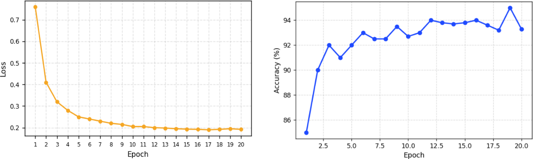
The training loss for Model A declines sharply in the initial epochs, then stabilizes after epoch 10. This indicates rapid learning followed by convergence. The loss plateaus below 0.2, showing a strong model fit without signs of overfitting (Figure 6).
Training loss (left) and validation (right) curves for Model A

Validation accuracy improves steadily across epochs, peaking at 94.5% and stabilizing above 93.8%, with minor fluctuations typical of validation variance. This suggests robust generalization capabilities.
4.1.2. Model B (MobileNetV3 on uncoated screws)
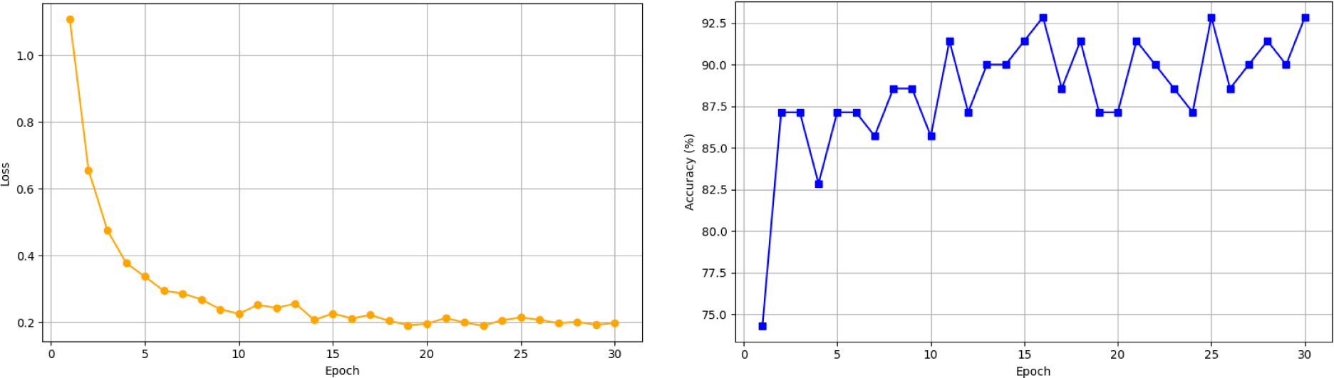
Model B, trained on uncoated steel screws with MobileNetV3-Small, shows slower initial convergence but ultimately achieves strong performance. While the training loss decreases more gradually (Figure 7), it stabilizes after around 20 epochs. Despite increased variability in surface appearance, the model continues to show consistent improvement.
Training loss (left) and validation accuracy (right) curves for Model B

Validation accuracy peaks at 92.5 % (Figure 7), confirming MobileNetV3’s efficiency despite its compact architecture. Oscillations are visible but do not indicate overfitting. This performance, combined with the lightweight model design, makes it a solid candidate for embedded or low-power deployment.
4.2. Classification performance
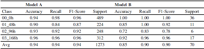
Each model was evaluated on its respective validation set using the same metrics. The prediction accuracy ranges from 72% to 96% (averaging 85%-94% for Model A and Model B, respectively). The classification accuracy is a bit better than that achieved by (Reference Elamparo, Telan and IbarraElamparo et al., 2023), a Mask R-CNN for rust detection on galvanized iron sheets. The classification model based on four rust levels (no rust, slightly visible rust, visible rust, and heavy visible rust) has an average accuracy of 80%.
A detailed classification report is presented in Table 1, including precision, recall, and F1-score per class.
Validation classification metrics for models A and B

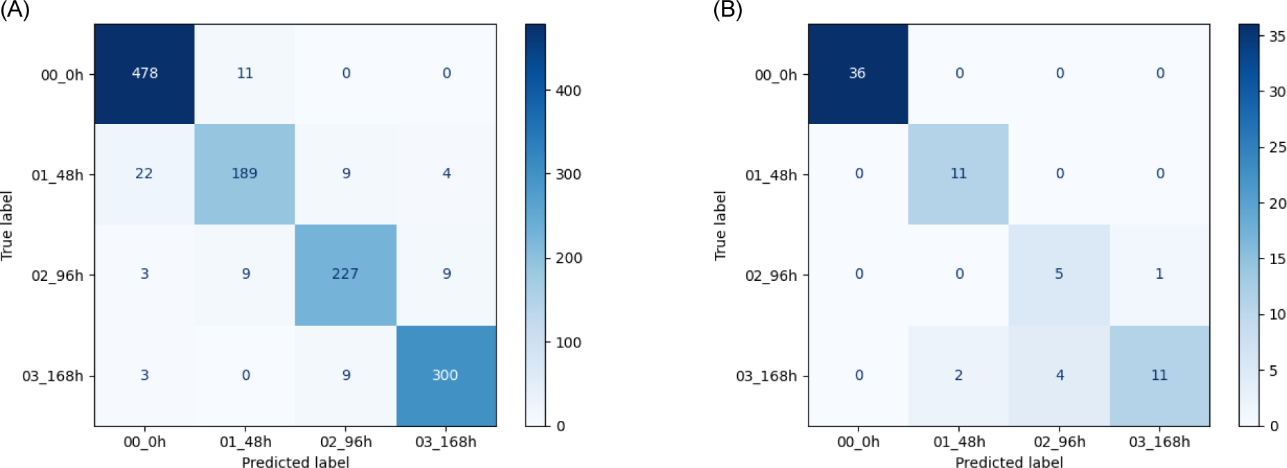
Confusion matrix for model A (left) and model B (right)

The confusion matrices in Figure 8 provide insight into the classification behavior of both models. For Model A (ResNet-18), most predictions lie on the diagonal, indicating that the network correctly recognizes most samples in each rust-exposure class. Misclassifications mainly occur between 48h and 96h, when corrosion patterns are visually similar due to the gradual transition from early to intermediate rust stages. The 0h and 168h classes show almost no confusion, confirming that extreme rust levels are easier to distinguish.
For Model B (MobileNetV3-Small), the overall structure of the matrix shows similar trends. The model achieves perfect classification for the 0h class, and strong performance for 168h, where high corrosion levels are visually distinct. Errors again appear primarily between 48h and 96h, with the limited number of samples in the uncoated dataset amplifying this effect. The small dataset size leads to occasional misclassifications at intermediate stages, yet overall performance remains strong, demonstrating MobileNetV3-Small’s suitability for low-data conditions.
Together, these matrices confirm that both networks reliably identify clearly separated corrosion levels. At the same time, intermediate stages remain the most challenging because of the subtle changes in texture and color as rust progresses.
4.3. Evaluation on real-world samples
In addition to validation on the labeled dataset, several individual screw images collected under real conditions outside the controlled salt-chamber setup were tested with the trained ResNet-18 model. These samples were preprocessed in the same way as the training data and passed through the network for classification.
A lightweight Python script was used to load images and infer their corrosion class. Although no large, annotated real-world dataset was available, this test served as a practical proof of concept. Figure 9 shows an example of a clean screw correctly classified as class 0 (0h exposure), and a rusted screw predicted as class 3 (168h exposure).
Real-world image of an unrusted (class: 0, left) and rusted screw (class: 3, right)

These results suggest that the model can generalize to non-laboratory images to some extent. However, due to the limited number of test samples available, this evaluation remains qualitative. Further testing with larger, annotated real-world datasets is needed to assess the model’s robustness and reliability in practical deployments.
As an additional perspective, generating synthetic screw images using generative AI techniques (such as diffusion models or vision-language models) could help augment the test dataset when physical samples are limited. This approach, while still experimental, could provide valuable diversity and controlled variability, enabling better evaluation of the model’s behavior across different conditions.
5. Conclusions
This work presented a complete pipeline for rust-level classification of screws using deep convolutional neural networks. Two separate datasets were constructed under controlled conditions: one with zinc-coated screws and one with uncoated steel screws. Each was used to train a tailored model architecture—ResNet-18 and MobileNetV3-Small, respectively.
The results demonstrate that both models can effectively distinguish between four levels of corrosion with high accuracy (94.5% for ResNet-18 and 92.5% for MobileNetV3). Despite differences in dataset size and surface conditions, the training process remained stable, and generalization performance was consistent.
However, several limitations affect the robustness of the current approach. The overall image quality was suboptimal, with variations in framing and lighting due to the experimental setup. The zinc-coated screws also corroded faster than expected, resulting in fewer usable images at intermediate rust levels and lower salt visibility in some stages. Additionally, the dataset remained relatively small and limited to synthetic lab conditions, reducing its representativeness for real-world industrial scenarios.
Future work could include acquiring higher-quality images, improving control over salt deposition, expanding the dataset to include more screw types, materials, and corrosion patterns, and deploying the models in real maintenance environments. Fine-grained segmentation and domain adaptation techniques could further enhance performance and applicability.




 Open access

