
16.1 Introduction
Spontaneous conversational speech appears to be produced in spurts. Rather than being a fluent, uninterrupted flow of words, it is jerky and irregular: Hesitations, false starts, and repetitions are the norm, not the exception (Chafe, Reference Chafe1994; Goldman-Eisler, Reference Goldman-Eisler1961; Shriberg, Reference Shriberg2001). In a technical sense, periods of fluent articulation are intermittent: Speech is comprised of short bursts of articulatory activity interrupted by periods of inactivity. Despite this, it has been suggested that there is a phrasal rhythm of speech, and that an oscillatory mechanism generates this rhythm. This notion might be inspired by the observation that syllables and stress can have fairly regular periodicities, or perhaps from the occurrence of low-frequency neural oscillations phase-locked to syllabic events in speech perception (Chapter 3; Boucher et al., Reference Boucher, Gilbert and Jemel2019; Peelle and Davis, Reference Peelle and Davis2012). But is there evidence for temporal regularity in speech production on longer timescales?
This chapter is organized as follows. First, some empirical data regarding phrase-timescale temporal patterns will be presented. Then, the hypothesis that an oscillatory mechanism directly generates these temporal patterns is considered. Lastly, I present a model in which phrase timing is epiphenomenal: Temporal patterns arise indirectly from mechanisms that govern conceptual-syntactic organization.
To preview the conclusions: Evidence for an oscillatory control mechanism is not so strong. Furthermore, such a mechanism may be implausible from a neurophysiological perspective (see discussion in Meyer et al., Reference Meyer, Sun and Martin2019). Instead, I argue that temporal patterns on phrasal timescales result from the actions of systems that organize conceptual and sensorimotor representations. A model is presented in which phrase-timescale intermittency arises from the reiteration of processes that govern the formation of coherent states among conceptual and syntactic systems. In this model, conceptual and syntactic systems transition back and forth between disordered and ordered states, analogous to repeated rapid-cooling processes. For a variety of reasons, these systems may fail to achieve a sufficiently ordered state, inducing a hesitation. Various control parameters can be manipulated to adjust the rate of hesitation. This mechanism provides a more empirically consistent understanding of phrase-timescale temporal patterns in speech production than oscillator-based models.
There are several important limitations of scope for the reader to make note of. First, this chapter addresses timescales at or greater than the prosodic word – metrical-/stress-related temporal patterns should not be confused with the phrasal ones of interest here. Second, I am concerned with speech that is produced spontaneously. This means that speakers themselves generate the conceptual content, usually in turns with a conversational partner, and that neither initiation nor termination of articulation is cued by an external system such as a metronome or experimental stimuli (of course, the environment along with conversational partners are complex external systems that influence initiation and termination of articulation). Third, I focus on the generation of temporal patterns, that is, the production of speech, as opposed to perception – oscillations in neuronal local field potentials that occur while perceiving speech do not constitute evidence that oscillations govern speech generation (see Chapter 6). Lastly, I do not discuss theories of hierarchical prosodic phrase structure, because prosodic-structural theories do not directly specify mechanisms that generate temporal patterns. Whether such theories could be adapted to do so is an open question (see Chapter 20).
One important terminological point should be made up front regarding use of the term rhythm, which is the topic of this volume. In a generic sense, rhythm can be used to describe any temporal pattern whatsoever. But in this generic usage, the term rhythm lacks bite: All speech has some temporal pattern. I prefer to reserve the term rhythm for the presence of a regular temporal pattern. Most dictionary definitions agree with this qualifier, and many researchers use rhythm to imply some form of temporal regularity in the recurrence of events. For example, Nolan and Jeon (Reference Nolan and Jeon2014) describe a notion in which a pattern must repeat and the temporal intervals of repetition must be regular. Likewise, the original notion of metrical rhythm classes (Abercrombie, Reference Abercrombie1967; Pike, Reference Pike1945) was assessed using direct measures of temporal isochrony in syllables or feet (Lehiste, Reference Lehiste1977; Ohala, Reference Ohala, Fant and Tathm1975). The reason that Turk and Shattuck-Hufnagel (Reference Turk and Shattuck-Hufnagel2013), in their discussion of rhythm, state that speech “is not periodic on the surface … [and] that no constituent recurs at regular temporal intervals” is because regularity is implied by the word rhythm.
When one insists on a notion of regularity for using the term rhythm, it raises an important question: What makes a temporal pattern “regular”? There is no nonarbitrary way to distinguish between temporal patterns that might be interpreted as regular and those that might not. Some specific examples of this problem will arise below. It follows that any answer to the question of whether speech exhibits temporal regularity is subjective – it depends on an arbitrary decision about what constitutes regularity. For this reason, rather than trying to determine the phrasal rhythm of speech, a more productive line of inquiry is to explore what sorts of models can generate empirically consistent patterns.
16.2 Some Empirical Data
Spontaneous conversational speech is produced in spurts. In more abstract terms, spurts are periods of high activity separated by periods of inactivity. In speech, this means that speakers tend to produce one to several words or phrases and then briefly hesitate or pause. As observed in Chafe (Reference Chafe1994: 57): “Anyone who listens objectively to speech will quickly notice that it is not produced in a continuous, uninterrupted flow but in spurts.” A schematic illustration of the spurt-like nature of speech is shown in Figure 16.1A, which depicts speech activity patterns from 10 relatively long turns randomly selected from the Switchboard NXT corpus (Calhoun et al., Reference Calhoun, Carletta and Brenier2010; Godfrey et al., Reference Godfrey, Holliman and McDaniel1992) (henceforth SWB). Speech and nonspeech periods are shown with dark gray and white intervals, respectively; filled pauses (uh, um) are shown with light gray.
The spurt-like temporal pattern of speech.
Depiction of speech activity intervals from randomly selected conversational turns from the SWB corpus: white is silence, dark gray is speech, and light gray is filled pause.

Markov chain transition probabilities.
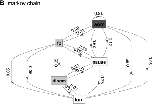
Figure 16.1(B) Long description
The nodes represent the states, and the arrows represent the probabilities of moving from one state to another. The numbers on the arrows indicate the transition probabilities.
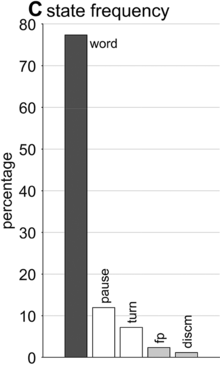
State occupation percentages.
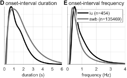
Gaussian kernel densities of unit onset-to-onset duration and frequency from the SWB and IU (intonational unit) corpora.

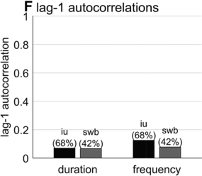
Lag-1 autocorrelations of consecutive interval durations and frequencies.
In a qualitative sense, periods of speech activity in some ways may resemble other natural phenomena that are intermittent, such as firewood popping, the acoustic emission of paper crumpling, or even earthquakes. These are instances of so-called crackling noise, which is associated with a class of systems that exhibit power-law distributions of event sizes or rates (Clauset et al., Reference Clauset, Shalizi and Newman2009; Sethna et al., Reference Sethna, Dahmen and Myers2001). Another natural example of intermittency arises in some circumstances when fluids transition back and forth between laminar and turbulent flow. Even fairly simple dynamical systems such as the Lorentz system can exhibit intermittency, and there are a number of different ways it can arise (Pomeau and Manneville, Reference Pomeau and Manneville1980). In such systems, rate or size distributions are similar across a wide range of scales. However, unlike the above examples, the durations of speech activity periods vary in a range that is no more than two orders of magnitude (i.e., 100–102), and so it is difficult to assess whether these events exhibit a power-law distribution of sizes. Whether or not the physical examples are good analogies to speech is hard to say, since we know so very little about the mechanisms that generate speech.
What is known, however, is that spontaneous speech rarely remains fluent for an extended time. Figure 16.1B shows a Markov model representation of speech-state transition probabilities obtained from the SWB corpus. This model makes the simplifying assumptions that (i) speech activity is always in one of a set of mutually exclusive states and (ii) there are probabilities that the speaker transitions between each pair of states. The model is useful to examine not because it is a realistic model of behavior but because it helps us visualize and quantify the temporal persistence of fluency. Note that due to polysemy, a set of certain words (e.g., yeah, no, okay) were counted as discourse markers when occurring pre- or post-pausally, and otherwise as words (see below for additional methodological details). The transition probabilities of the Markov model show that nearly one out of every five words is followed by something other than a word, such as a pause (12%), a filled pause (5%), or a change of turn (5%). Furthermore, Figure 16.1C shows that the overall occupancy rate of the word state is only about 75% across the corpus. The 0.81 self-transition probability of the word state entails that when a speaker initiates a phrase, there is less than a 50% chance that the phrase will consist of more than three words before being interrupted.
To quantify variability in phrasal temporal patterns, I examine durational patterns associated with periods of fluent speech activity, or spurts. I define a spurt as a sequence of words that does not include a hesitation (pause or filled pause); also, pre-/post-pausal discourse markers are excluded from the analyses, since these are often associated with turn changes. The periods of time between the onsets of consecutive spurts within a turn were extracted from the SWB corpus – here these are referred to as spurt intervals. The frequencies associated with spurt intervals are merely the reciprocals of their durations (see Greenberg et al., Reference Greenberg, Carvey, Hitchcock and Chang2003, for similar and additional methods for analyzing temporal patterns).
Researchers familiar with abstract theories of prosodic structure might wonder: Would it not be better to examine the intervals between onsets of some familiar prosodic units, such as phonological phrases or intonational phrases? The answer to this question could very well be no, since it is not very common for such phrases to be produced without any internal hesitation; moreover, there is no ground truth parsing of speech into higher-level prosodic structure, and there is substantial disagreement about the nature of the structure: Theories range from positing a hierarchy of unique levels (Beckman and Pierrehumbert, Reference Beckman and Pierrehumbert1986; Hayes, Reference Hayes, Kiparsky and Youmans1989; Nespor and Vogel, Reference Nespor and Vogel2007; Selkirk, Reference Selkirk1986), to positing just a couple of levels with recursive organization (Ito and Mester, Reference Ito and Mester2007; Wagner, Reference Wagner2010), to positing no structure whatsoever (Tilsen, Reference Tilsen2019b, Reference Tilsen2022). Nonetheless, for purposes of comparison, Figures 16.1D–F show data associated with intonation units, obtained from the Santa Barbara Corpus of Spoken American English (SBC; Du Bois et al., Reference Du Bois, Chafe, Meyer, Thompson and Martey2000) and manually labeled by Inbar et al. (Reference Inbar, Grossman and Landau2020). I refer to the intervals between intonation units as IU intervals.
Spurt and IU interval durations are highly variable. Gaussian kernel densities of the interval durations are shown in Figure 16.1D for spurt intervals (gray lines) and IU intervals (black lines). Although the distributions do have modal durations (about 0.75 and 1.0 s, respectively), the ranges of the intervals are quite wide: from about 0.5 s to 4 or 5 s. These fairly wide ranges suggest that it may be difficult to accurately predict when the next spurt will begin merely from knowledge of when the current one began. Notice that the distribution of spurt intervals is also skewed rightward, indicating that there are more long spurts than would be expected from a normal distribution of inter-spurt intervals. Figure 16.1E shows effectively the same patterns, after the durations are transformed to frequencies. Note that the modal frequencies do not correspond to the modal durations because Gaussian kernels applied to nonlinearly related variables (such as duration and frequency) do not match.
Furthermore, consecutive spurt/IU intervals are not strongly correlated. Figure 16.1F shows the lag-1 autocorrelations of spurt/IU interval durations and frequencies. The lag-1 autocorrelation is the value of a variable correlated with the next observation of that variable. In other words, lag-1 autocorrelation quantifies to what extent one interval is correlated with the next. This is a useful measure to examine because some of the variability in interval durations may arise from differences across speakers, turns, or contexts – yet these sources of variance should have minimal influence on the correlation of adjacent intervals. Since the lag-1 autocorrelation can only be calculated from consecutive intervals (i.e., three consecutive spurts or IUs), and since some turns are comprised of just one or two spurts/IUs, only a portion of the intervals can be included in the analysis (about 68% and 42% for the two corpora). Notice that lag-1 autocorrelations are positive, but they are fairly small. Even the largest (r ≈ 0.15 for IU frequencies) entails that the frequency of one IU accounts for less than 3% of the variation in the next.
What do the empirical patterns tell us about the regularity of phrasal timing in spontaneous speech? Recall that one fifth of the time a word will be followed by something other than a word, and that 50% of spurts will consist of three words or fewer; these observations call into question whether it is sensible to look for regularity in the first place: If long stretches of speech without pauses, discourse markers, or changes of turn are relatively uncommon, what exactly should one measure to detect phrasal regularity? Second, regarding the duration/frequency distributions of spurt and IU intervals, it is my opinion that the presence of a modal (most common) duration/frequency does not itself constitute evidence for regularity of temporal patterns. Rather, the widths and shapes of the distributions are important: Whereas very narrow, symmetric distributions might support the idea that there are regular temporal patterns, very broad, skewed distributions do not. Some of the variance in the corpus-wide distributions of interval durations/frequencies might be attributed to variation between speakers/turns; in that case, temporal regularity would lead us to expect substantial lag-1 autocorrelations between consecutive intervals within a turn, but this does not appear to be the case either.
There are some potential criticisms of the methodology for obtaining the empirical measures of spurt timing. For one, it was not possible to automatically detect spurt-internal discourse markers and other forms of disfluency (such as cutoffs, repetition disfluencies, or simply hesitatory lengthening while maintaining a speech posture), and so some spurts may be erroneously longer than they should be. However, this criticism does not apply to the manually labeled IU units, which also exhibit high variability and low lag-1 autocorrelation. It also seems unlikely that even if these criticisms could be addressed, interval distributions would become substantially narrower.
Nonetheless, any qualitative interpretation of the patterns is necessarily subjective: How narrow should a distribution be, or how high should an autocorrelation be, in order to infer the existence of a phrasal rhythm? Instead of trying to answer the question of whether the empirical patterns provide evidence for a regular phrasal rhythm, I pursue a related question: What are the necessary properties of a periodic control mechanism that would be consistent with the observed temporal patterns? This is the approach pursued in the next section.
16.3 Oscillation as a Direct Rhythm Mechanism
Here I consider oscillation as a possible generating mechanism for phrasal temporal patterns. Such a mechanism could be motivated from the fact that there is evidence for oscillation on sub-phrasal timescales, that is, timescales of syllables/stress. For example, metrically regular patterns are produced more quickly and with fewer errors than irregular ones (Tilsen, Reference Tilsen2011); in tongue twister paradigms, the reverse pattern holds: More errors occur in metrically regular sequences (Myers and Watson, Reference Myers and Watson2021). Stuttering is diminished in speech entrained to a metronome (Chapter 46; Brady, Reference Brady1971). More generally, cultures have a pervasive habit of putting speech to a beat. There are several models in which oscillatory mechanisms are involved in generating sub-phrasal rhythms (for some examples, see O’Dell and Nieminen, Reference O’Dell and Nieminen1999; Saltzman et al., Reference Saltzman, Nam, Krivokapic and Goldstein2008; Tilsen, Reference Tilsen2009, Reference Tilsen2019a). The fact that oscillation appears to be relevant on the sub-phrasal scale raises the question of whether it is also involved on larger temporal scales, that is, those of phrases.
A number of researchers have developed oscillator-based models of phrasal rhythmicity, but none of these readily applies to the generation of spontaneous speech. For example, there are models of phrasal oscillation in special experimental contexts with metronome-entrained speech (Cummins and Port, Reference Cummins and Port1998; Port, Reference Port2003; Tilsen, Reference Tilsen2009), but there is little evidence to suggest that these models generalize to spontaneous speech. There are also oscillator models that are applied to neural activity evoked in speech perception (Bourguignon et al., Reference Bourguignon, Molinaro and Lizarazu2019; Giraud and Poeppel, Reference Giraud and Poeppel2012; Inbar et al., Reference Inbar, Genzer, Perry, Grossman and Landau2023; Rimmele et al., Reference Rimmele, Poeppel and Ghitza2021), but these do not necessarily claim that oscillations generate phrasal temporal patterns in production, only that such patterns arise in perceiving speech. Notably, although it has been argued that low-frequency delta-band (<1–2 Hz) activity observed in electroencephalography (EEG)/magnetoencephalography (MEG) supports perceptual chunking of phrases, it has alternatively been argued that the low-frequency oscillation arises from pauses in connected speech (Zhang et al., Reference Zhang, Zou and Ding2023). Chapters 3, 5–7, and 9 further address the role of neural oscillation in speech processing. Some recent theories (Benítez-Burraco and Murphy, Reference Benítez-Burraco and Murphy2019; Tilsen, Reference Tilsen2019b) have proposed that oscillations organize neural processes that construct conceptual-syntactic representations, but neither of these holds that neural oscillations are directly responsible for the initiation or termination of motor actions (Chapter 6). There currently exists no implemented model of phrasal oscillation in spontaneous speech.
16.3.1 Empirical Evidence for Phrasal Rhythmicity
To my knowledge, there are just two studies in the literature that use empirical evidence to support the claim that phrasal rhythms in production are associated with an oscillatory mechanism. One of these is a recent study of IUs (Inbar et al., Reference Inbar, Grossman and Landau2020). The authors examined manually labeled IUs from spontaneous speech in a variety of languages, including the SBC (included in the analyses above). To investigate temporal patterns, they conducted a clever analysis using a phase consistency measure developed for studying neural oscillations (Vinck et al., Reference Vinck, van Wingerden, Womelsdorf, Fries and Pennartz2010). The analysis works as follows (see Chapter 15). First, a wideband amplitude envelope of the speech signal is split into two-second windows centered on the onset of each IU, and these windows are Hann-windowed. Then a Fourier transform is applied to each window, and the consistency of the phase of each complex Fourier coefficient component is calculated by the pairwise phase consistency (Vinck et al., Reference Vinck, van Wingerden, Womelsdorf, Fries and Pennartz2010). This value is effectively an average angular correlation between the phases estimated from all windows, for a given frequency component. Intuitively, this measure tells us how similar the phases of a particular Fourier component are across a dataset. Inbar et al. (Reference Inbar, Grossman and Landau2020) found that there was a peak in the consistency around 1 Hz (note that two-second windows entail effective frequency bins of 0.5 Hz, which are wide in relation to the typical durational range of IUs). They interpret this finding by stating that “prosodic units … give rise to a low-frequency rhythm” and that “speakers express their developing ideas at a rate of approximately 1 Hz.” These statements seem to suggest that a phrasal oscillation governs speech production, although it is unclear whether the authors contend that organization into IUs is the cause or effect of the phrasal rhythm.
There are several potential criticisms of the Inbar et al. (Reference Inbar, Grossman and Landau2020) study that call into question how strongly it supports the idea that there is a phrase-timescale oscillation that governs speech. First, the pairwise phase consistency analysis method they used is more complicated than the simpler method of examining the distributions and autocorrelations of interval durations/frequencies; if these simpler methods show broad distributions, then the discrepancy between methods warrants an explanation. Second, the manual labeling of IUs makes a presupposition about the existence of such units; this presupposition cannot be independently validated from a ground truth parsing of the signal because the units themselves are hypothetical entities (Chafe, Reference Chafe1994). Third, since the analysis considers all windows, it represents an aggregate over speech produced at different times and from different speakers, as opposed to a temporally local correlation between successive intervals. Fourth, and most importantly, the interpretation of the presence of a peak in phase consistency suffers from the same problems of subjectivity and arbitrariness that were discussed above in relation to interval duration distributions: The width and shape of the distribution must also be considered, not just the presence of a mode. In my estimation, the phase consistency functions for each of the six languages examined in Inbar et al. (Reference Inbar, Grossman and Landau2020) are not very sharply peaked: The half-bandwidths of the peaks in most cases appear to extend from approximately 0.25 to 2 Hz (or, 4 to 0.5 s), which is a fairly broad range. Indeed, the results could very well be interpreted as evidence against temporal regularity on the phrasal timescale.
A second study that also argues for a phrasal oscillation is Stehwien and Meyer (Reference Stehwien and Meyer2022). The authors examined human-annotated intonational phrases and intermediate phrases from a corpus of German radio news. They conducted autocorrelation analyses on subsets of data in which intonational phrases were collected according to their durations, using one-second bins. The autocorrelation was conducted on binary time series with time steps of 0.001 s, in which the value 1 indicated the offset of an intermediate phrase. Using this approach, they found significant autocorrelation at lags in the range of 610–1,200 ms – a frequency range of 0.83–1.64 Hz. They also report that the standard deviation of differences in adjacent phrase durations was 1.11 s. Stehwien and Meyer (Reference Stehwien and Meyer2022) interpret the findings as “evidence for an association between acoustic patterns in speech and periodic electrophysiological sampling time windows of the auditory system” – this association might be taken to imply that auditory oscillations are responsible for periodicity in the acoustic output of speech (although the authors do not explicitly state this).
Some of the same criticisms that bear on Inbar et al. (Reference Inbar, Grossman and Landau2020) apply to Stehwien and Meyer (Reference Stehwien and Meyer2022). Specifically, the intonational and intermediate phrase parsings are contestable because they are hypothetical units, and most importantly, it is not clear whether the frequency range of significant lags (0.83–1.64 Hz) should be viewed as relatively narrow or relatively broad. The phrase-to-phrase jitter of 1.11 s indeed seems to be quite large. Furthermore, it is important to note that analyses of broadcast news speech may not generalize to spontaneous speech: Broadcast news speech is produced by speakers with specific training, it is often guided by a transcript, and it may have its own stylistic characteristics, including context-specific intonational patterns.
16.3.2 Assessment of a Model of Oscillator-Driven Phrasal Timing
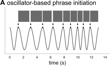
To further assess the idea that phrasal timing patterns can be explained by an oscillatory mechanism, one can explore the predictions of an oscillator-based model. Because there is no well-developed spontaneous speech phrasal oscillator model in the literature (see Chapter 6), it is necessary to borrow an idea from the metrical oscillator models. A typical aspect of these models is that the initiation of a syllable/foot is triggered when the oscillator reaches some particular phase of its cycle (see, for example, Saltzman et al., Reference Saltzman, Nam, Krivokapic and Goldstein2008; Tilsen, Reference Tilsen2009). In other words, the oscillator initiates the production of a unit at some particular moment that is consistent from one cycle to the next. Applying this idea to a phrasal oscillator entails that the reciprocal of a spurt interval (or whatever interval one might define) should correspond to the frequency of the oscillator, as shown in Figure 16.2A. I will assume that the oscillator has a constant frequency within each cycle (note, this assumption does not sacrifice generality because a constant frequency can be viewed as an average of instantaneous frequency over one cycle). Given these assumptions, can an oscillatory mechanism generate the empirical interval densities?
Analysis of a phrase oscillator model.
Schematic illustration of phrase initiation in a phrasal oscillator model.

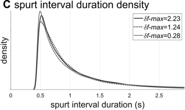
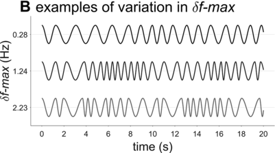
Examples of phrasal oscillation for extremal and medial values of δf-max.

Spurt-interval densities for the extremal/medial values of δf-max.
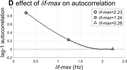
Lag-1 autocorrelations as a function of δf-max.
A crucial model parameter to consider relates to how much one will allow the oscillator frequency to vary from one cycle to the next. This parameter is expressed here with δf-max, the maximal absolute change in frequency from one cycle to another. Figure 16.2B contrasts phrasal oscillators with three different values of δf-max, that is, different degrees of time-varying random frequency variability. Low values of δf-max result in fairly regular oscillations, high values in irregular oscillations. Consider that if δf-max is unbounded, oscillator frequency can change arbitrarily from one cycle to another, and the model is overly powerful: It can generate any imaginable pattern of jitter in phrasal intervals. Indeed, allowing for large δf-max seems to subvert the meaning of regularity and periodicity that is associated with the concept of “oscillation.”
What value of δf-max is most consistent with the empirical data? To answer this question, some additional details of the model must be fleshed out. Specifically, a strategy is needed for determining how f changes from one cycle to the next. Here the change is modeled as a random walk, but boundary constraints [fmin, fmax] that correspond to the 5th and 75th percentiles of empirical spurt frequencies are imposed. This means that for each cycle i, a value δfi is randomly selected from the interval [−δf-max, +δf-max], and is added to the frequency of the previous cycle, that is, fi = fi-1 + δfi. If the resulting value falls outside of the bounds [fmin, fmax], a new random value is selected until the resulting frequency is within bounds. In model simulations, 101 values of δf-max were examined, ranging from fmin to fmax. For each value of δf-max, 10,000 consecutive intervals were generated. This Monte Carlo approach to modeling phrasal rhythm provides a time series of adjacent spurt durations, from which lag-1 autocorrelations can be calculated.
The interval duration densities (n=10,000) associated with low, high, and intermediate values of δf-max are shown in Figure 16.2C. The densities show that δf-max does not have a substantial effect on the shape or width of the expected distribution of interval durations. The reason for this is that the random walk eventually explores the entire space between the frequency bounds; it merely does so more quickly with larger δf-max. It is noteworthy that the shapes of the duration distributions are skewed rightward, not unlike the empirical ones (solid black line). In contrast to the frequency distributions, δf-max has a strong effect on lag-1 autocorrelation, shown in Figure 16.2D. Here one can see that a large δf-max of around 1.35 Hz is needed to generate the fairly small empirical lag-1 autocorrelation of r = 0.15.
Overall, the model simulations suggest that in order for a phrase oscillator to generate lag-1 autocorrelation patterns that match the largest values observed in the corpora, then δf-max would need to be around 1.35 Hz. Can this value be interpreted as support for or against the hypothesis that a phrasal oscillator drives phrase initiation? To me, the value seems to allow a fairly drastic change in frequency from cycle to cycle – about 70% of the allowed frequency range (or 24% of the period range). In any case, without a specific model of the neural mechanisms that give rise to the oscillation, it is hard to assess how realistic this variation would be.
There are of course several potential criticisms of the model, which might call into question how strongly inferences can be drawn from it. One criticism might be that stochastic effects in the triggering of phrase initiations are not included; perhaps there is a variable delay from the triggering phase to phrase initiation. Including a random delay would allow for lower δf-max to attain empirically observed autocorrelations, but the magnitude of this random deviation would need to be quite large. Perhaps the most important criticism is that it is too strong to assume that every cycle of oscillation generates a spurt – maybe spurt initiations can skip cycles if the preceding spurt has not been completed. To implement a model of that sort, additional mechanisms would be needed to govern spurt termination. I leave the exploration of this larger parameter space to future work. Nonetheless, the main conclusion from the simulations is that a phrasal oscillator would seem to need an overly powerful ability to change frequency in order to generate empirically consistent temporal patterns.
The second reason why direct oscillatory control of phrasal timing may not be plausible is a neurophysiological one: The frequency range necessary to account for empirical interval distributions is unlikely to be associated with a single neurogenic origin. It seems reasonable to expect that if there exists a phrasal oscillator, its neural origins would have a unitary origin. Our current knowledge of how neural oscillations arise may not be consistent with this expectation. Consider that even a very conservative estimate of the range of IU frequencies from the SBC corpus is about 0.25–2 Hz. Although occasionally one can find superficial descriptions of neural oscillation frequency bands in which this range of values is labeled as δ-band (delta-band), many of the more detailed analyses distinguish between different delta bands, due to the fact these have different apparent origins and behavioral correlates. There is in fact no widespread agreement about the functions of different oscillations in different bands. For instance, Buzsáki and Draguhn (Reference Buzsáki and Draguhn2004) distinguish between delta (1.5–4 Hz), slow 1 (0.5–1.5 Hz), and slow 2 (0.20–0.5 Hz) oscillations. Or, Jensen et al. (Reference Jensen, Spaak, Zumer, Supek and Aine2019) describe delta as (1–4 Hz) and note that a proposed neurogenic mechanism involves slow inhibitory neurotransmitter effects in cells that project from the thalamus to the cortex, which form part of a thalamo-cortical circuit. Other oscillatory bands, such as theta, alpha, beta, gamma, and high gamma, are each proposed to arise from different mechanisms. To my knowledge, no one has proposed that there exists a functionally coherent 0.25–2 Hz band of oscillatory activity with a single neurogenic mechanism (see also Chapters 3 and 35). Moreover, it is a bit puzzling that the strongest delta rhythms tend to be observed during sleep (Buzsáki and Draguhn, Reference Buzsáki and Draguhn2004). Thus, one should be cautious in jumping to the conclusion that just because there is oscillatory neural activity across a range of low frequencies, it supports the notion of a phrasal oscillator.
16.4 Conceptual-Syntactic Coherence as the Source of Phrase-Timescale Temporal Patterns
Instead of thinking of phrasal timing as something that is controlled directly, perhaps phrase initiation can be understood as an indirect consequence of other control mechanisms, namely those that are involved in conceptual and syntactic processes. In other words, perhaps speakers do not care at all about when phrases are initiated: There is no system that directly governs phrasal timing.
In this section I describe a theoretical framework for understanding speech production – the oscillators and energy levels framework – developed in Tilsen (Reference Tilsen2019b). Then I present simulations of a model in this framework, in which there are mechanisms that give rise to intermittency of speech activity. Finally, I explain how this model can be used to describe transitions to and from fluent speech. The key ideas of the model are that there are special systems that monitor the states of conceptual and syntactic systems; and furthermore, whenever conceptual and syntactic systems reach a noncoherent state, these monitoring systems induce a reorganization process that results in hesitation, that is, a temporary halt of content-related speech activity. The notion of coherency of state may be unfamiliar to readers and is elaborated and exemplified below.
Section 16.4.1 provides a highly condensed overview of some of the basic aspects of the oscillators and energy levels theory, which is too large in scope to describe in its entirety here. Section 16.4.2 shows with model simulations how intermittency can arise. Only the most relevant details are made explicit here, and the reader should view this section as a proof-of-concept, as opposed to a comprehensive presentation of the model. For readers who are interested in the details of the model, a full exposition of all parameters, equations, model code, and examples of how to run the model are available at https://github.com/tilsen/oel_intermittency.git.
16.4.1 Overview of the Parallel Domains – Oscillators/Energy Levels Theory
In the oscillators/energy levels theory, all entities involved in speech production are dynamical systems with the potential for oscillatory activity; their states can be described by variables of phase, instantaneous frequency, and amplitude. There are two primary domains of organization: the conceptual-syntactic domain (cs-domain), and the gestural-motoric domain (gm-domain). These are referred to as parallel domains for two reasons: (i) system states in both domains evolve at the same time and (ii) the mechanisms of organization in the two domains are highly similar. Figure 16.3 illustrates various aspects of the model that are discussed below.
Overview and example of the oscillators/energy levels model.
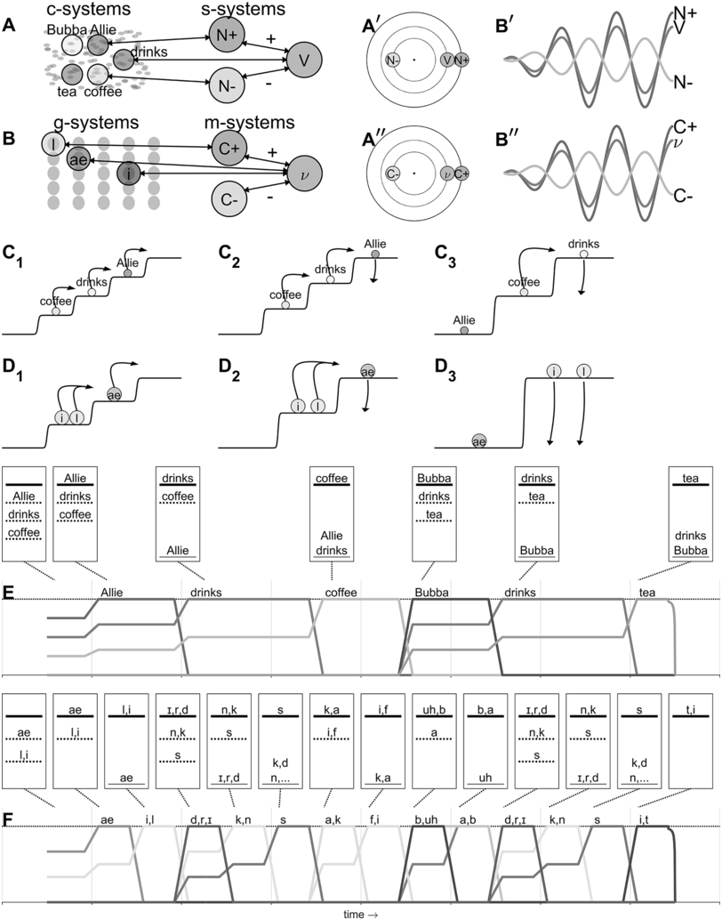
The example utterance is Allie drinks coffee, Bubba drinks tea. (A) Concept systems couple with syntactic systems, which organize them into relative phase configurations (Aʹ) that describe patterns of oscillation (Aʹʹ). (B) Gestural systems couple with motor-sequencing systems, which organize them into relative phase configurations (Bʹ) that describe patterns of oscillation (Bʹʹ). (C1, C2, C3) Activation potentials for a sequence of states of conceptual-syntactic organization. (D1, D2, D3) Activation potentials for a sequence of states of gestural-motoric organization. (E) Activation variable trajectories for conceptual-syntactic systems. Relative energy hierarchies are indicated. (F) Activation variable trajectories for gestural-motoric systems.

Figure 16.3 Long description
Panel a. A network-like diagram shows relationships between different entities like Bubba, Allie, drinks, tea and coffee. The N plus and N minus symbols and "V" suggest a possible concept of positive and negative influences or states. Panel b. A similar waveform structure is labeled N plus, V, N minus, C plus, C minus and nu. Panel c. Three diagrams show transitions between states, with arrows indicating the direction of change. The entities like Allie, drinks and coffee are involved in these transitions. Panel d. These diagrams are similar to panel C. Panel e. A three-step line representation of words including Allie, drinks, coffee, bubba, drinks and tea. A table shows a sequence of states. The states are denoted with letters including a e, l, i, r, d, n, k, s, k, a, i, f, uh and b, a representing different states. Panel f. A multistep line representation depicts the progression of states, including a e, l, i and more.
In the conceptual-syntactic domain, there are many instantiations of two basic types of systems: concept systems (c-systems) and syntactic systems (s-systems), as represented in Figure 16.3A. Instances of both types are argued to correspond to neural populations. In the case of c-systems, the neural populations that instantiate a particular c-system are distributed across cortical multimodal association areas and interact with primary sensory and motor areas. An example of a c-system is [COFFEE]. This system interacts with various sensorimotor information that encodes, for example, the smell and taste of coffee, its visual appearance, and motor patterns that we have for interacting with it. The neural populations that instantiate [COFFEE] are also expected to overlap with populations associated with related concept systems, such as [TEA] or [CUP]. Because of this, there are varied, diverse interactions between c-systems. Note that there are important differences (as discussed in Tilsen, Reference Tilsen2019b) between c-systems that are more grammatical in nature (such as a c-system for [SINGULAR] or [3RD PERSON]) and those that are more lexical (such as [COFFEE] or [DRINK]) – I will not delve into these aspects of the theory here (see Chapter 6 and Shattuck-Hufnagel, Reference Shattuck-Hufnagel and Redford2015, for alternative perspectives).
Syntactic systems (s-systems), in contrast to c-systems, are neural populations that are more cortically localized and that interact in highly constrained ways. S-systems are defined in part by how they phase-couple to other s-systems. For example, in the production of a simple subject-verb-object (SVO) sentence such as Allie drinks coffee, the subject system (N+) and the verb system (V) are attractively phase-coupled, while the object noun system (N−) and verb system are repulsively phase-coupled. This pattern is shown in the network structure of Figure 16.3A and the resulting relative phase configuration is shown in Figure 16.3Aʹ, with corresponding oscillations in Figure 16.3Aʹʹ. Importantly, c-systems can phase- and amplitude-couple to s-systems, and because of this property, s-systems can organize c-systems into stable relative phase configurations. The relative phase configurations that arise between c-systems indirectly in this way are held to evoke relational meaning experiences. In other words, the meaning of Allie drinks coffee is an experience associated with a particular relative phase configuration. Crucially, this experience is argued to arise when the relevant systems exhibit strong phase coherence, meaning that their relative phases are relatively stable over time.
Similarly, in the gestural-motoric domain, there are two types of systems: gestural systems (g-systems) and motor-sequencing systems (m-systems), as shown in Figure 16.3B. G-systems are similar in some respects to the gestures of articulatory phonology (Browman and Goldstein, Reference Browman and Goldstein1992), but note that in Figure 16.3, for visual simplicity phonetic symbols are used to refer to oral articulatory gestures. In the same way that s-systems organize c-systems into stable relative phase configurations, motor-sequencing systems (m-systems) couple to g-systems and thereby bring them into particular configurations. In this domain, rather than evoking meaning experiences, relative phase configurations dictate coordinative relations between gestures. M-systems also function to group g-systems into sets that are sequentially selected, as theorized in the selection-coordination theory of speech production (Tilsen, Reference Tilsen2014, Reference Tilsen2016). Importantly, the mechanisms that govern c- and s-system interactions in the conceptual-syntactic domain are highly similar to those that govern g- and m-system interactions in the gestural-motoric domain.
All four types of systems can be characterized by two state variables: phase (φ) and activation (or its discrete counterpart, excitation [e]). The dynamical laws that govern these variables depend on which dynamical regime a given system is in. There are three regimes that are distinguished: (i) an inactive state, in which a system is effectively ignored because its excitation variable is too low; (ii) an active state, in which a system exhibits non-negligible but nonetheless low levels of excitation and relatively incoherent oscillation; and (iii) an excited state, in which a system obtains high levels of excitation and exhibits relatively self-coherent oscillation – that is, an oscillation with stable frequency and amplitude. Coherence in this sense can be quantified via autocorrelation: When a system oscillates with stable frequency and amplitude, there will be a strong peak in its short-time autocorrelation, or equivalently a large peak in its power spectrum.
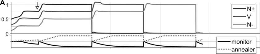
The roles of the three regimes can be understood by considering what happens prior to initiation of speech, and continuing through fluent production. Figure 16.3 panels C1–C3 illustrate activation potentials for the first three epochs of conceptual-syntactic organization in the production of the utterance Allie drinks coffee, Bubba drinks tea; likewise, panels D1–D3 illustrate the potentials for the first three epochs of gestural-motoric organization. (Note that the step functions shown in the panels can be viewed as potentials in the technical sense: They are functions of system activation and the negative of their first derivative is the force that acts on the system; however, the step functions shown here are designed primarily for illustrative purposes rather than quantitative accuracy.) The lowest level of the potential is the ground level – systems that occupy this level are in an active state but are not excited. Systems occupying all above-ground levels are excited. The highest level of the potential is the selection level – c-systems that occupy the selection level exert strong forces on associated g-systems, and g-systems that occupy the selection level exert strong forces on vocal tract systems (which are roughly equivalent to the tract variables of task dynamics [Saltzman and Munhall, Reference Saltzman and Munhall1989]).
In panel C1, the three c-systems of the first clause ([Allie], [drinks], and [coffee]) are initially organized into a relative excitation hierarchy that corresponds to the order in which they will be selected. Other c-systems that may be involved in the utterance are active but not yet excited. The most highly excited system [Allie] is not yet at the selection level. The arrows in C1 indicate what happens after the configuration in epoch C1 stabilizes: [Allie] is promoted to selection level, and the remaining systems [drinks] and [coffee] are promoted to the next highest level, as shown in C2. The arrows in C2 indicate what happens next: When feedback (either internal or external) regarding the selection of [Allie] reaches a threshold, [Allie] is demoted to ground level and the remaining systems are promoted. The demotion of selected systems and the promotion of remaining systems iterate until the next clause, where [Bubba], [drinks], and [tea] are organized and undergo a similar sequence of operations.
Similarly, in panel D1, three gestural systems associated with [Allie] are organized into a relative excitation hierarchy with all three systems initially below the selection level. This organization process is understood to happen contemporaneously with the organization of the c-system [Allie]. Notice that [l] and [i] occupy the same level of the excitation hierarchy. This reflects the observation that these oral gestures will be selected together and coordinated (i.e., co-selected; see Tilsen, Reference Tilsen2016). (Note that c-systems can also be co-selected, and that the system labeled [drinks] in C1–C3 is more precisely understood as a co-selection of the c-system [drink], [3RD PERSON], [SINGULAR], and [PRESENT TENSE].) The arrows in D1 indicate what happens next: The systems associated with [ae] (a lingual gesture and a glottal adduction gesture) are promoted to selection level, as shown in D2, and this drives changes in vocal tract systems/effectors. Eventually, internal and external feedback lead to the demotion of [ae] and the promotion of the next set of gestures, resulting in the excitation configuration shown in D3.
The entire sequence of conceptual-syntactic and gestural-motoric epochs and corresponding activation trajectories for the utterance Allie drinks coffee, Bubba drinks tea are represented in Figure 16.3, panels E and F, respectively. The activation trajectories are idealized representations of the activation state variables of the c- and g-systems over the course of producing the utterance – note that when adopting this quantized representation, activation is relabeled excitation. Discrete epochs of the c- and g-system relative excitation hierarchies are shown above the activation trajectories. The top-most line in each epoch is the selection level; the bottom solid line is the ground level.
The sequence of relative excitation states that occurs in the course of producing an utterance such as the one above can be understood as a dynamical production trajectory: It describes the trajectory of a complex system (consisting of many component systems) in a high-dimensional space, with those systems evolving according to change rules that incorporate force-like interactions between systems and an environment.
The above exposition provides a highly condensed description of the oscillators/energy levels theory (see Tilsen, Reference Tilsen2019b). The key idea for current purposes is this: Before a system can be promoted to selection level, its state has to become relatively stable and coherent. This applies both to the epoch in which systems are initially organized below selection level and to subsequent epochs in the production of the utterance. Specifically, coherence entails that there is a relatively strong peak (or multiple strong peaks) in the autocorrelation or power spectrum of the system state; this will only be present when the system frequency and amplitude are relatively stable.
Loosely speaking, the model holds that prior to utterance initiation, there is a pandemonium of disorganized and unstable oscillation among c-systems and s-systems (i.e., the short-term power spectra of these systems lack clear peaks). Through competitive interactions between systems, the disorganized state rapidly organizes into a highly ordered one in which a small set of c-systems and s-systems exhibit coherent oscillations. This evolution of the full system can be conceptualized as a cooling process. Special-purpose coherence-monitoring systems recognize the achievement of this high degree of coherence and induce processes that result in the generation of movement (which is controlled through similar processes involving gestural and motoric systems). Transitions from disordered, noncoherent states to ordered, highly coherent states occur repeatedly throughout spontaneous speech production.
16.4.2 How Intermittency of Phrase Initiation Arises
This section presents simulations of a model in the oscillators/energy levels theoretical framework. The aim of the model is to show one possible mechanism by which the intermittency of speech activity might arise. The model is intended to illustrate this particular mechanism, rather than generate the statistics of speech activity periods. Nonetheless I will discuss how the model could be used to do this.
The key idea of the model is that hesitations in spontaneous conversational speech can occur when conceptual-syntactic or gestural-motoric configurations become noncoherent (or, degenerate). When this happens, the system resets itself and the speaker hesitates. For simplicity, the model simulates only concept (c-) and syntactic (s-) system states; gestural/motoric organization would exhibit similar sorts of behaviors. Note that model code, descriptions of all model equations and parameters, and examples of how to use the model are available online (https://github.com/tilsen/oel_intermittency.git).
One key point to make about the model is that it requires a surroundings (or “environment”), which is what causes c-systems to become active in the first place (c-systems can also cause other c-systems to become active, but this never occurs in a vacuum). In any real context, the environment is always complex and dynamic, and therefore the forces that c-systems experience will vary in complicated ways over time. In the simulations below, these environmental forces are simplified by making them constant throughout an utterance, yet randomly determined from one simulation run to another. Moreover, a condition is imposed that the utterance is always a SVO sequence. This condition does not sacrifice the generality of inferences about intermittency; it merely serves to allow for more direct comparisons of model behavior as certain parameters are varied.
A second key point to make is that there are a number of sources of stochasticity in the model, and that these are ultimately responsible for the (non)occurrence of degenerate states. Specifically, degenerate states occur when s-systems fail to attain a relative excitation configuration with certain properties. Those properties are, first, that mutually exclusive s-systems cannot occupy the same level of the relative excitation potential, and, second, that there should not exist an unoccupied level of the potential. These circumstances can arise from stochasticity in initial conditions, from interactions between c-and s-systems, or from environmental forces. Furthermore, the forces that are associated with the excitation potential are modulated by an annealing system: These forces are initially weak but strengthen over time. The annealer state is analogous to inverse temperature in that regard, and the formation of a coherent state can be viewed as a cooling process. By increasing the strength of excitation potential forces in this way, there is a period of time when stochastic forces on s-systems may or may not prevent them from coming to occupy the excitation levels in a canonical way. Similarly, whenever a selected system is demoted, there is an annealing process that again allows for stochastic effects on excitation organization.
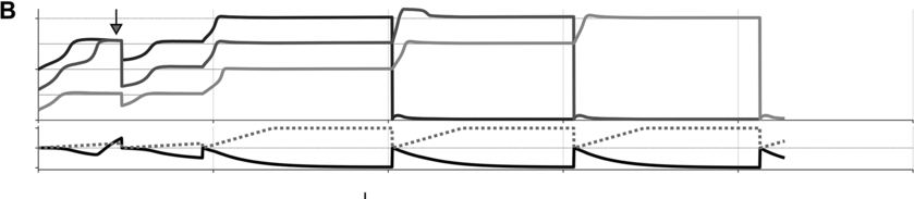
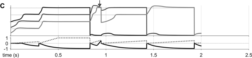
Some examples of these phenomena are exemplified in Figure 16.4 below. Panels A–C show selected system state variables from several example utterances. In each panel, the top portion shows the activation states of the three s-systems in the utterance (N+, V, N-), and the bottom portion shows the states of the s-system annealer (dashed line) and the excitation coherence monitor (solid line). Example A shows system state trajectories when no degeneracy occurs. Notice that the s-system excitations grow initially but soon stabilize in separate wells of the excitation potential. Subsequently, when the excitation coherence monitor reaches a threshold value (around the time indicated by the arrow), it induces a reorganization of the excitation potential, such that each s-system is promoted. The next reorganization occurs when feedback for the selected syntactic system reaches a threshold value. Iterated reorganizations consist of demoting a previously selected system to the ground level, and promoting all remaining above-ground systems.
Simulations of the intermittency mechanism and parameter effects.
Panels A–C show (top) syntactic system activation trajectories for three syntactic systems and (bottom) annealer (dashed line) and monitor trajectories (solid line).
Canonical production trajectory.
Degenerate excitation state occurring before initial coherence, occurring at the time indicated by the arrow.

Degenerate excitation state occurring within sequence production, occurring at the time indicated by the arrow.

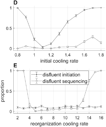
Effects of initial cooling rate and reorganization cooling rate parameters on the likelihood of disfluent initiation and sequencing.

Figure 16.4(D, E) Long description
Graph D plots the disfluent proportions versus initial cooling rate. The initiation line originates at (0.8, 1), falls, and rises to terminate at (0.8, 1.8), and the sequencing line originates at (0.8, 0), fluctuates and terminates at (1.8, 0.2). Values are estimated. Graph E plots the disfluent proportion versus the reorganization cooling rate. The line for disfluent sequencing initially falls, remains stable and then rises. The line for disfluent initiation remains stable along the x-axis.
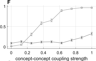
Effect of concept–concept activation-coupling strength on disfluency likelihoods.

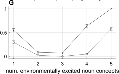
Effect of the number of environmentally excited concept systems on disfluency likelihoods.
Examples B and C show two different cases in which a degenerate excitation configuration arose in a simulation, at the time indicated by the arrows. B is an example of noncoherence in initiation, or disfluent initiation. Here the degenerate state occurs before the first selection: Both {N+} and {V} occupy the same energy level. The detection of the degenerate state by the monitor induces a reset of s-system activation and a restart of the annealing process. This case corresponds to a hesitation before the initiation of a phrase. C is an example of intra-sequence noncoherence, or disfluent sequencing. Here the degeneracy occurs after the demotion of the first selected system, before {V} is promoted to selection level. The monitor decreases the activation of the above-ground systems and the annealing process is restarted. This case corresponds to a hesitation within a phrase.
Various model parameters influence the occurrence rates of disfluent initiation and disfluent sequencing; moreover, these parameters can be given behavioral/functional interpretations that allow for the model to generate a variety of phenomena. Selected parameter effects are shown in Figure 16.4, panels D–G. Panel D shows that when the initial cooling rates are too high or too low, sequence initiation is more likely to be disfluent. The likelihood of disfluent sequencing (assuming that initial coherence occurred) is mostly unaffected by the initial cooling rate, but note that it increases a bit with high initial cooling rates. Similarly, panel E shows that reorganization cooling rates that are too low or too high lead to disfluent sequencing. The initial cooling rate parameter can be interpreted as the degree of motivation that a speaker has to begin speaking. The model suggests that the more urgency speakers feel to initiate an utterance, the more likely they are to hesitate when trying to begin the utterance. The reorganization cooling rate parameter can be interpreted as a speech rate control parameter: Higher cooling rates produce faster speech, but are more likely to result in disfluency.
Panel F shows how fluency depends on the strength of activation-coupling forces between concepts. Note that concept–concept activation interactions are randomly selected values on the interval [−1,1] with symmetric sign, reflecting the notion that concept interactions are mutually excitatory or inhibitory but generally asymmetric in strength. When these interactions are increased in strength, c-systems are more likely to interfere with each other; this can prevent the achievement of a stable s-system configuration because of c-s activation coupling. Panel G shows how fluency depends on the number of environmentally excited noun concepts. When this number is less than the number required for an SVO utterance, disfluency rates are higher. Conversely, when the number increases, there is greater interference with s-systems and disfluency rates increase. These effects connect with the idea that, like humans, the model has limited working memory.
In sum, the model provides proof-of-concept that the intermittency of speech activity may derive from factors that influence whether conceptual and syntactic systems are likely to organize into states with particular properties. Moreover, the model provides a number of parameters that can be plausibly related to forms of behavioral variation, such as speech rate, as well as contextual variation, such as the number of concepts that are activated by the environment. Importantly, the model shows how we might more realistically conceptualize phrasal timing: Rather than being governed directly by an oscillatory mechanism, temporal patterns on phrase timescales are indirect consequences (epiphenomena) of processes involved in conceptual-syntactic organization.
Before concluding, it is worth discussing a number of shortcomings of the model in its current implementation. First, the excitation dynamics are implemented with discrete operations, but a more sophisticated model would allow for such dynamics to emerge from interacting dynamical systems, or from a spatial organization of systems (e.g., see Grossberg, Reference Grossberg1987). The premise that speech can be idealized as a sequence of discrete operations on states is useful but ultimately needs to be derived from more fundamental systems. Second, in order to achieve coherent initial states, s-systems in the model cannot have arbitrary initial excitation values. Thus, it must be assumed that there exists some mechanism that constrains initial s-system values to certain ranges. Third, the model presupposes that the environment fully determines a particular syntactic configuration. In other words, the canonical syntactic form of an utterance does not emerge stochastically from the state of the environment. Fourth, not only excitation but also relative phase configurations should also be monitored for coherence, and relative phase degeneracies should introduce hesitations. Extensions of the model to address these limitations are currently underway. Once these environmental forces are modeled appropriately, it will be possible for the model to generate conversational turn-timescale output with speech-like intermittency statistics.
Summary
In spontaneous conversational speech, phrases are initiated intermittently. Evidence for an oscillatory mechanism that directly controls phrasal timing is inconclusive. Instead, intermittency in phrasal timing may be an epiphenomenon of processes involved in conceptual-syntactic organization. The sources of intermittency could derive from systems that monitor the coherence of conceptual and syntactic systems.
Implications
Without appropriate controls, statistical characterizations of phrasal timing patterns are unlikely to shed light on the nature of speech production in spontaneous conversational speech. It is crucial to consider syntactic and conceptual factors in phrasal timing. Furthermore, speaker- and discourse-context-related factors must also be considered.
Gains
Our understanding of speech production has been improved by recognizing that the timing of phrases depends on many factors, some of which relate to the conceptual content and syntactic organization of speech. We can avoid mistakenly attributing phrasal timing patterns to the effects of a dedicated control mechanism.


 Open access