

1. INTRODUCTION
Many natural phenomena, including thermodynamic, geophysical, and biological systems, can be described as reservoirs with inputs (e.g., mass, energy, information) that produce a related output. The behavior of these systems depends fundamentally on the extent to which they integrate their inputs. This is often characterized by a response time, or ‘memory’, that is related to the capacity of the reservoir and the characteristic input and output rates. This timescale determines how quickly the system can respond to a perturbation.
When a gradual forcing is applied, an ‘equilibrium response’ can be defined as the state at which the system would be in equilibrium with the forcing at any given instant. This state evolves with the forcing. However, because the system has a memory of its previous states, the actual system state lags the equilibrium response by an amount that depends on its response time. This basic concept has major implications in the context of a changing climate system, which has subcomponents that respond on a wide range of timescales. One of the most striking examples is the rate of surface warming in response to anthropogenic CO2 emissions. Transient warming lags the equilibrium response due to the vast thermal inertia of the ocean (e.g., Wigley and Schlesinger, Reference Wigley and Schlesinger1985). In turn, warming surface temperatures constitute a gradual forcing for other systems with long response times: lagged responses have also been investigated for sea-level rise (e.g., Meehl and others, Reference Meehl2005) and forest die back (Jones and others, Reference Jones, Lowe, Liddicoat and Betts2009), among many other environmental responses to warming.
In this paper, we investigate these concepts for the case of the retreat of mountain glaciers in a warming climate. Previous studies have noted that many glaciers are out of equilibrium with the modern climate and thus committed to additional change (e.g., Bahr and others, Reference Bahr, Dyurgerov and Meier2009; Mernild and others, Reference Mernild, Lipscomb, Bahr, Radić and Zemp2013; Marzeion and others, Reference Marzeion2017, Reference Marzeion, Kaser, Maussion and Champollion2018). Indeed, standard mass-balance measurements report surface mass balance over the evolving glacier area (e.g., WGMS, 2017), and so the widely noted negative mass balance of most of the world's glaciers (e.g., IPCC, Reference Stocker2013; Medwedeff and Roe, Reference Medwedeff and Roe2017) necessarily implies they are out of equilibrium. A number of studies have gone a step further, calculating glacier extents that would be in equilibrium with recent climate observations. Such studies have targeted South Cascade Glacier, Washington (Rasmussen and Conway, Reference Rasmussen and Conway2001), Haig Glacier, Canada (Adhikari and Marshall, Reference Adhikari and Marshall2013), Morteratsch Glacier, Switzerland (Zekollari and others, Reference Zekollari, Fürst and Huybrechts2014; Zekollari and Huybrechts, Reference Zekollari and Huybrechts2015), Great Aletsch Glacier, Switzerland (Jouvet and others, Reference Jouvet, Huss, Funk and Blatter2011), as well as collections of glaciers in the Alps (Lüthi and others, Reference Lüthi, Bauder and Funk2010; Carturan and others, Reference Carturan2013) and Bhutan (Rupper and others, Reference Rupper2012). These studies have highlighted a striking discrepancy between current and equilibrium glacier geometries in specific settings; here, we explore the fundamental controls on this response. We first illustrate the basic behavior of glacier retreat with a simple model, and introduce metrics for characterizing the discrepancy between the evolving transient and equilibrium length responses. We then present experiments in which we use several additional models of varying complexity to evaluate how ice dynamics, glacier geometry, and climate variability control the transient glacier response to gradual warming.
1.1. Illustrating disequilibrium with a simple glacier model
A mountain glacier can be conceptualized as an open system with memory: it integrates mass accumulated across its surface into a reservoir of ice, and this reservoir adjusts its extent to maintain a balance between input in the accumulation zone and output in the ablation zone. The simplest representation of this behavior is a first-order differential equation for fluctuations of length, L′, around a steady state,  $\bar L$, caused by mass-balance perturbations, b′:
 $$\displaystyle{{{\rm d}{L}^{\prime}} \over {{\rm d}t}} + \displaystyle{{{L}^{\prime}} \over \tau} = \; \beta {b}^{\prime},$$
where
 $$\beta = \displaystyle{{\; {\rm \;} \bar L} \over H}.$$
H is a characteristic ice thickness and τ is the glacier response timescale, given by
 $$\tau = - H/b_{\rm t},$$
where b t is the (negative) annual mass-balance rate at the terminus. β is a geometric parameter that scales the length responses to mass-balance perturbations; as we will see, it is related to the glacier's length sensitivity. In this model, the glacier's length is the only degree of freedom, so Eqn (1) is a mass-conservation statement equating ice-volume change to imbalance between input and output rates (e.g., Jóhannesson and others, Reference Jóhannesson, Raymond and Waddington1989).
The basic model represented by Eqns (1) and (2) has been widely used to explore glacier responses to climate perturbations (e.g., Jóhannesson and others, Reference Jóhannesson, Raymond and Waddington1989; Harrison and others, Reference Harrison, Elsberg, Echelmeyer and Krimmel2001; Oerlemans, Reference Oerlemans2001, Reference Oerlemans2007; Roe and O'Neal, Reference Roe and O'Neal2009). While various formulations for the response timescale and glacier-sensitivity parameters have been proposed, members of this family of models all resolve the same basic behavior. For an instantaneous mass-balance change Δb at t = 0, the glacier asymptotically approaches a new geometry described by  $\bar L + \Delta L$, where accumulation and ablation are again balanced. The solution of Eqn (1) for this case is
 $${L}^{\prime}(t) = \Delta L(1 - {\rm e}^{ - t/\tau} ),\; \; $$
where
 $$\Delta L = \; \tau \beta \Delta b.$$
 Another important analytical solution to Eqn (1) is the case of a linear trend in mass balance ( $\dot b \equiv {\rm d}b/{\rm d}t$), starting at t = 0:
 $${L}^{\prime}(t) = \tau \beta \dot b[t - \tau (1 - {\rm e}^{ - t/\tau} )].$$
 For t ≫ τ, Eqn (4) approaches  ${L}^{\prime}(t) = \; \tau \beta \dot b(t - \tau )$. Thus, at long timescales, there is a lag of τ behind the length at which the glacier would remain in equilibrium with the climate as it changes. We refer to this evolving length as the glacier's equilibrium response, defined by
 $${L}^{\prime}_{{\rm eq}}(t) = \tau \beta \dot bt.$$
Figure 1a shows the responses of a glacier with an arbitrary timescale τ to mass-balance changes imposed instantaneously or as linear trends. Results are plotted as normalized by τ in time and |ΔL| in length. Solid lines show the transient length changes and dashed lines show the equilibrium responses (Eqn (5)). Four rates of forcing are shown: the same total mass-balance change Δb is applied instantaneously (black), or gradually applied over periods of 2τ (blue), 6τ (red), and 50τ (gold).
The response of a simple glacier model to a step function and sustained trends in climate forcing. (a) Normalized length response to a climate forcing. Solid lines show the transient response, dashed lines show the instantaneous equilibrium length. The climate forcing is applied as a step function (black), and as a trend over periods of 2τ (blue), 6τ (red), and 50τ (gold), where τ is the glacier response timescale. (b) Degree of disequilibrium in normalized length. (c) Fractional equilibration, which proceeds identically for all climate trends until the forcing stops.
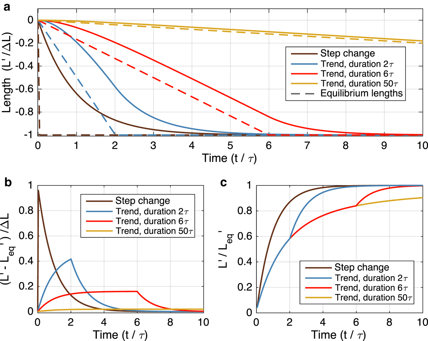
We will refer to the difference between transient and equilibrium responses (Lʹ and  $L_{\rm eq}^{\prime}; solid and dashed lines) at any given time as the ‘disequilibrium’. Figure 1b shows this metric for each forcing, again normalized by |ΔL|. For mass-balance trends, the degree of disequilibrium approaches a constant (see the case of the 6τ trend in Fig. 1b), which depends on the rate of forcing. The response to a slow trend (50τ, gold curves in Fig. 1) approaches a limiting case in which the glacier responds quasi-statically, and its degree of disequilibrium is negligible.
During a warming period, the degree of disequilibrium is a measure of a glacier's overextension, and thus the amount of additional retreat that is already guaranteed even with no further climate change. Climate researchers have introduced the concept of ‘committed warming’ as a quantity describing the warming that will still occur even if anthropogenic forcing stabilized (e.g., Hansen and others, Reference Hansen1985; Wigley and Schlesinger, Reference Wigley and Schlesinger1985; Wigley, Reference Wigley2005); similar metrics exist for committed sea-level rise and ice-sheet loss (e.g., Meehl and others, Reference Meehl2005; Price and others, Reference Price, Payne, Howat and Smith2011; Goldberg and others, Reference Goldberg, Heimbach, Joughin and Smith2015). The reference state used to define the committed change varies in the literature. In this paper, we use the term ‘committed retreat’ to refer to the additional retreat that must occur for the glacier to reach equilibrium should warming stop abruptly at a given time. In this sense, its magnitude is equivalent to the degree of disequilibrium, though committed retreat also has a time dependence: once the forcing stops, the realization of committed retreat is still governed by τ.
The ratio  ${L}^{\prime}/{L}^{\prime}_{{\rm eq}}$ is another way to express a glacier's lagged response to a climate trend. At any instant in time, this is the fraction of the total (equilibrium) adjustment that the glacier has attained for the amount of climate change that has already occurred. We will refer to this as ‘fractional equilibration’. It is a useful measure of the committed retreat in the context of the changes that have already been observed. For example, a fractional equilibration of 33% would mean that twice as much retreat as has already occurred is committed to happen in the future, if the climate stopped changing at that moment. Figure 1c shows the evolution of ${L}^{\prime}/{L}^{\prime}_{{\rm eq}}$. Note that the fractional equilibration progresses identically for all three rates of gradual forcing (blue, red, and gold curves) until the forcing stops.
Figure 1 highlights some very general behavior discussed in the previous section: systems with memory produce a lagged response when a gradual forcing is applied, and their degree of disequilibrium can be significant when the duration of the forcing is similar to the response timescale. Most mountain glaciers have response times between ~10 and 100 years (e.g., Jóhannesson and others, Reference Jóhannesson, Raymond and Waddington1989; Oerlemans, Reference Oerlemans2001) – similar in order to the duration of anthropogenic climate forcing to date (~100 years; IPCC, Reference Stocker2013). The results from this simple model show that neither the instantaneous nor the quasi-static limits realistically describe recent glacier changes, nor those that can be expected in the near future. However, applying these concepts to observations or projections requires using models that capture the relevant dynamics and can incorporate glacier and climate observations. To evaluate the important factors for understanding glacier disequilibrium in today's climate, we present several experiments using idealized glacier geometries forced with gradual warming trends. In the next section, we describe the four models used, and the idealized glacier settings. We then compare the hierarchy of models to evaluate the importance of ice dynamics. Next, we investigate the role of glacier geometry by assessing response times across a range of geometries, and by considering uncertainty in ice thickness. Finally, we consider several issues that climate variability can bring to estimating or modeling glacier disequilibrium.
2. METHODS
2.1. Linear models
The simplest model we consider in our experiments is given by Eqns (1) and (2). However, this model assumes that the glacier has a single dynamical stage: mass-balance fluctuations cause an immediate tendency on the glacier length, L′, damped exponentially on the timescale τ. Roe and Baker (Reference Roe and Baker2014) evaluated the ability of Eqn (1) to emulate the behavior of a shallow-ice flowline model as a function of frequency, f. Equation (1) performs well at low frequencies (f ≪ 1/τ), but the single dynamical stage exaggerates the high-frequency response. Roe and Baker (Reference Roe and Baker2014) developed a new linear model that incorporates three stages of glacier response: changes in ice thickness drive changes in ice flux that, in turn, drive changes in glacier length. Their model takes the form of a third-order ordinary differential equation:
 $$\left( {\displaystyle{{\rm d} \over {{\rm d}t}} + \displaystyle{1 \over {\epsilon \tau}}} \right)^3{L}^{\prime} = \displaystyle{1 \over {\epsilon ^3\tau ^2}}\beta {b}^{\prime},$$
where τand β are defined as above, and  $\epsilon = 1/\sqrt 3 $. Following the terminology in Roe and Baker (Reference Roe and Baker2014), we will refer to Eqns (1) and (6) as one-stage and three-stage models, respectively.
The three-stage model is governed by the same response-time parameter as the one-stage, but in a different functional form (i.e., it arises from the same geometric considerations, but is not an e-folding timescale). As noted above, the two models differ primarily at high frequencies; however, these differences remain relevant at long timescales when the forcing is a continuous trend. This is evident in the long-term limits of the one-stage and three-stage responses to a linear mass-balance trend,  $\dot b$, starting at t = 0. The one-stage solution is given by Eqn (4), and the three-stage solution is
 $$\eqalign{{L}^{\prime}\left( t \right) = \tau \cdot \left[ {1 - \displaystyle{{3\epsilon \tau} \over t}\left( {1 - {\rm e}^{ - t/\epsilon \tau}} \right) + {\rm e}^{ - t/\epsilon \tau} \left( {\displaystyle{t \over {2\epsilon \tau}} + 2} \right)} \right] \cdot \beta \dot bt.}$$
 For t ≫ τ, Eqn (7) approaches  ${L}^{\prime}(t) = \; \tau \beta \dot b(t - 3\epsilon \tau )$, indicating a greater lag behind the equilibrium response than the one-stage model. The fractional equilibration also highlights this difference. For each model, it is obtained by dividing Lʹ(t) (Eqn (4) for one-stage, Eqn (7) for three-stage) by the equilibrium length response ( ${L}^{\prime}_{{\rm eq}}(t)$; Eqn (5)). The factor ( $\tau \beta \dot bt$) drops out, leaving
 $$\left. {L^{\prime}/{{L}^{\prime}}_{{\rm eq}}} \right \vert _{1{\rm - stage}} = 1 - \displaystyle{\tau \over t}\; (1 - {\rm e}^{ - t/\tau} ),$$
and
 $$\eqalign{\left. {{L}^{\prime}/{{L}^{\prime}}_{{\rm eq}}} \right \vert _{3{\rm - stage}} = & 1 - \displaystyle{{3\epsilon \tau} \over t}\left( {1 - {\rm e}^{ - t/\epsilon \tau}} \right) \cr &+ {\rm e}^{ - t/\epsilon \tau} \left( {\displaystyle{t \over {2\epsilon \tau}} \; + 2} \right)}.$$
Both expressions depend only on the glacier's response time and the duration of the trend. The exponentials in Eqns (8) and (9) decay fastest, leaving terms proportional to 1/t in the long-time limit. However, the one-stage fractional equilibration asymptotes to 1 − τ/t, whereas the three-stage model asymptotes to a slower 1 − 3ετ/t approach to unity, on account of its greater lag behind the equilibrium response.
Several other analytical glacier models exist in the literature. For example, Harrison and others (Reference Harrison, Raymond, Echelmeyer and Krimmel2003) and Lüthi (Reference Lüthi2009) both developed dynamical models for area and volume fluctuations, which effectively have two stages of adjustment. Here we limit our selection of analytical models to the one-stage and three-stage frameworks. These provide a range in complexity, and allow for straightforward comparison as they are based on a common set of parameters, but, as discussed above, represent different assumptions about glacier dynamics.
2.2. Non-linear flowline models
In order to more comprehensively capture glacier dynamics, we use numerical models that explicitly represent ice deformation in response to driving stresses. These models ultimately stem from the Stokes equations,
 $$\nabla \cdot \sigma _{ij} = \; - \rho g_i$$
and
 $$\nabla \cdot u_i = 0,$$
where σ ij is the Cauchy stress tensor, ρ is the density of ice, g i is acceleration due to gravity, and u i are velocity components. Equation (10) expresses local balance between surface forces (stress gradients) and body forces (gravity) per unit volume of ice, while Eqn (11) expresses conservation of mass.
These equations are linked by a constitutive relation (Glen, Reference Glen1955) that relates driving stresses to strain rates  $\dot \varepsilon _{ij}$ (and therefore to velocities):
 $$\dot \varepsilon _{ij} = A\; S_{\rm e}^{n - 1} S_{ij}.$$
 A is the creep parameter that follows an Arrhenius relationship, which we hold constant (see Table 1), and we use a flow exponent of n = 3. S ij is the deviatoric stress tensor, defined as the Cauchy stress tensor minus its isotropic pressure component, and  $\; S_{\rm e}^2 \equiv (1/2)\; S_{ij}\; S_{ij}$ is a scalar effective stress. Finally, a continuity equation gives the evolution of local ice thickness, h:
 $$\displaystyle{{{\rm d}h} \over {{\rm d}t}} = b - \nabla \cdot {\bi F}{\rm,} $$
where b is the local surface mass-balance rate, and F is the vertically integrated ice flux. Here basal mass-balance terms are neglected, and it is assumed that bed geometry is constant in time, making Eqn (13) equivalent to the evolution of the ice surface.
Glacier and climate parameters for glaciers 1 and 2. The first group of parameters are those imposed in the flowline models, while the second group are calculated from the full-Stokes model and used to calibrate the linear models
The non-linear relationship between stress and strain (Eqn 12) can require significant numerical computation to solve in its full form, and for this reason, it is often advantageous to seek approximations to the Stokes equations. A common one in glaciology is the shallow-ice approximation (SIA), in which it is assumed that gravitational driving stress is balanced only by basal shear stress (e.g., Hutter, Reference Hutter1983). If x is the horizontal coordinate along a glacier flowline, z is the vertical coordinate, and s is the free ice surface, the driving stress is given by
 $$\sigma _{xz} = \sigma _{zx} = \; - \rho g_zh\displaystyle{{{\rm d}s} \over {{\rm d}x}},$$
and all other terms in the stress tensor are neglected. In contrast, ‘full-Stokes’ solutions make no such truncations and solve for the full stress state. The SIA is valid in the limit of shallow aspect ratios (H/L ≪ 1) and has been shown to be a reasonable approximation for mountain glacier geometries, although its performance declines for smaller glaciers and steeper bed slopes (e.g., Le Meur and others, Reference Le Meur, Gagliardini, Zwinger and Ruokolainen2004; Leysinger Vieli and Gudmundsson, Reference Leysinger Vieli and Gudmundsson2004; Adhikari and Marshall, Reference Adhikari and Marshall2011). Intermediate ‘higher order’ modeling frameworks exist that resolve some, but not all, additional stress components (e.g., Pattyn, Reference Pattyn2002; Hindmarsh, Reference Hindmarsh2004); in this study, however, we limit our comparison to SIA and full-Stokes models.
We run both a SIA and a full-Stokes model for a 2-D flowline, that is, assuming a constant glacier width and neglecting the influence of lateral boundaries. The SIA equations are integrated using finite differences and explicit time stepping (e.g., Oerlemans, Reference Oerlemans2001; Roe, Reference Roe2011) on a 25 m grid. For our full-Stokes simulations, we use the finite-element model Elmer/Ice (Gagliardini and others, Reference Gagliardini2013) with a horizontal element size of 25 m and ten vertical layers. For both models, we incorporate a simple Weertman-style sliding law (e.g., Weertman, Reference Weertman1964; Cuffey and Paterson, Reference Cuffey and Paterson2010):
 $$S_{\rm b} = Cu_{\rm b}^m. $$
S b is the basal shear stress, u b is the sliding velocity, and m is the Weertman exponent, or the inverse of the flow exponent n (i.e., m = 1/3). C is a constant sliding coefficient; however, note that the sliding velocity depends non-linearly on the basal shear stress.
We assume an altitude-dependent mass-balance function b(z) for the flowline models:
 $$b(z) = \bar P - \mu (\bar T_{z = 0} - {\rm \Gamma} z),$$
where  $\bar P$ is the mean annual accumulation, uniform across the glacier surface, and $\bar T_{z = 0}$ is the mean melt-season temperature at sea level. μ is a melt factor, relating mass balance to melt-season temperature, and Γ is the atmospheric temperature lapse rate.
2.3. Steady-state glacier geometries
Our model domains are idealized mountain glaciers with uniform bed slopes. We first consider two geometries: glacier 1 has a bed slope of tan (φ) = 0.2 (11.3°), and glacier 2 has a slope of tan (φ) = 0.1 (5.7°). Both have a maximum elevation of 2500 m a.s.l. (Fig. 2a). Table 1 displays the mass-balance and dynamical parameters used in the models. We use values for sliding and deformation parameters (C and A) that are considered typical for mountain glaciers (see, e.g., Budd and others, Reference Budd, Keage and Blundy1979; Oerlemans, Reference Oerlemans2001; Roe, Reference Roe2011). Our sliding relation (Eqn (15)) is a simplified version of that presented in Oerlemans (Reference Oerlemans2001), and subsequently in Roe (Reference Roe2011) and Roe and Baker (Reference Roe and Baker2014). These studies used C = (H s/f s)m, where H s is the ice thickness and f s is a sliding parameter, which they set at 5.7 × 10⁻²⁰ Pa−3 s−1 m2 following Budd and others (Reference Budd, Keage and Blundy1979). For simplicity, we treat H s as constant, set at 50 m for glacier 1 and 100 m for glacier 2. These values fall between initial mean thickness, and thickness after a 2°C warming (described in the next section). Using the above value for f s, this gives the constant sliding coefficients in Table 1. Our climate parameters are consistent with a temperate, maritime setting. With the values in Table 1, Eqn (16) gives equilibrium lengths of 6.55 km (glacier 1) and 13.1 km (glacier 2). Since an ice elevation–mass-balance feedback is not included, the equilibrium lengths are analytical functions of the mass-balance profile and the bed geometries.
Idealized glacier geometries and response to climate variability. (a) Equilibrium configuration for the two geometries used throughout this study. (b) Equilibrium ice thickness profiles generated with the full-Stokes (blue) and shallow-ice (red) models. The mean ice thickness for these profiles is used to determine τ in the one- and three-stage models. (c) Length response of all four models to white-noise interannual variability (σ T = 0.7 °C and σ P = 0.7 m a−1), for glacier 1. A 2.5 ka segment of a 10 ka model run is shown. The mass-balance anomaly is shown in the lower panel. (d) Power spectral density for the length responses to variability (glacier 1). Both (c) and (d) show that the one-stage response has more variance at high frequencies, but the other three models agree closely.
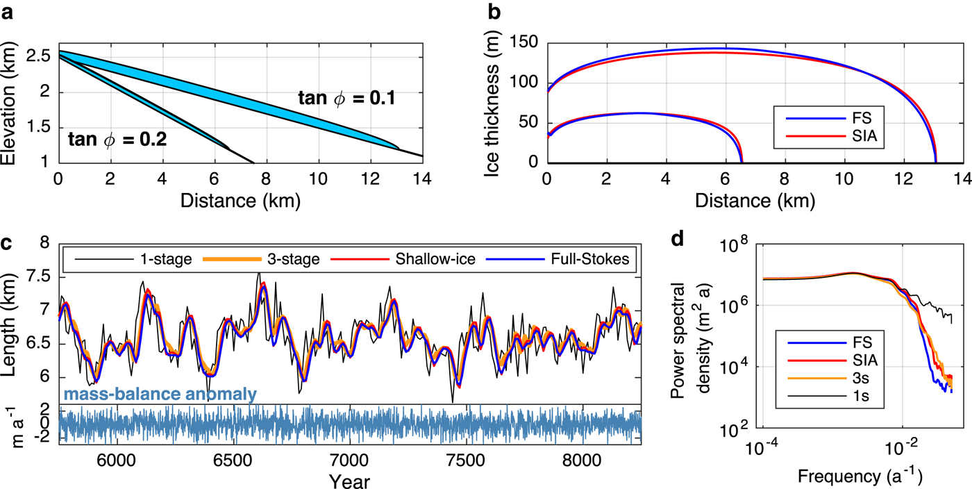
The full-Stokes and SIA models agree closely on their equilibrium thickness profiles, shown in Figure 2b. For the smaller, steeper glacier (1), mean ice thicknesses are 53 m (full-Stokes) and 54 m (SIA); and for the larger glacier (2), 123 m (full-Stokes) and 120 m (SIA). The similar thicknesses, in turn, imply good agreement on estimated response times (Eqn (2); τ = −H/b t). Using mean thicknesses for H, and with b t set by Eqn (16), Eqn (2) gives τ = 25 years for glacier 1, and τ = 57 years for glacier 2 (using full-Stokes thickness; 56 years for the SIA thickness). It should be noted that terminus ablation rate for both glaciers is lower than those observed on many glaciers; this is a consequence of their constant width.
We use the full-Stokes steady-state geometries to calibrate the one-stage and three-stage linear models (see the second group of parameters in Table 1). The elevation, temperature, and lapse rate parameters we have chosen (Table 1) dictate that some summer melt occurs at all elevations (i.e.,  $\bar T_{Z{\rm max}} \gt 0$), making Eqn (16) a continuous, linear function over our domain. This means that both temperature anomalies (Tʹ) and precipitation anomalies (Pʹ) correspond to uniform mass-balance anomalies. These mass-balance anomalies constitute the forcing for the linear models, and are given by
 $${b}^{\prime} = {P}^{\prime} - \mu {T}^{\prime}.$$
The linear model parameters presented here are a simple case of those derived for the one-stage model in Roe and O'Neal (Reference Roe and O'Neal2009) and for the three-stage model in Roe and Baker (Reference Roe and Baker2014), which were generalized to allow for a region where no melt occurs.
These synthetic geometries are meant to represent two generic mountain glaciers with distinct response times, rather than specific settings. However, to put their response times in context with glaciers around the world, we turn to Roe and others (Reference Roe, Baker and Herla2017, supplemental material), who estimated τ, according to Eqn (2), for 37 glaciers based on data from existing glacier inventories. For example, their timescale estimates for Blue Glacier in the Olympic Mountains (τ ~ 28 years) and Hintereisferner in the Austrian Alps (τ ~ 30 years) are comparable with our glacier 1 (τ = 25 years). Our glacier 2 (τ = 57 years) is similar in timescale to Saskatchewan Glacier in the Canadian Rockies, Gries Glacier in the Swiss Alps, or Storglaciären in northern Sweden (τ ~ 50, 59 and 60 years, respectively), among others. The largest glaciers in the Alps likely have even longer response times, with estimates for individual glaciers approaching or exceeding a century (cf. Lüthi and others, Reference Lüthi, Bauder and Funk2010; Roe and others, Reference Roe, Baker and Herla2017).
3. RESULTS
3.1. Model complexity
The one-stage model illustrated the basic response to a climate trend (Fig. 1); a next step is to investigate the responses of the more realistic models introduced in the previous section. Using a hierarchy of models, we can ask what is the simplest model that can accurately characterize a glacier's disequilibrium in a warming climate?
While our ultimate interest is retreat due to a warming trend, forcing the different models with stochastic climate variability is a good way to evaluate their relative performance as a function of frequency. We imposed 10 000 years of white noise (i.e., equal power at all frequencies) in both temperature and precipitation, with σ T = 0.7 °C and σ P = 0.7 m a−1. The resulting std dev. in mass balance is 0.78 m a−1, consistent with variability observed in maritime climates (e.g., Medwedeff and Roe, Reference Medwedeff and Roe2017). A 2500-year segment of our model output for the smaller glacier geometry is shown in Figure 2c; it is immediately clear that the one-stage model is an outlier, with much more high-frequency variability than the other three models. This is evident also in the power spectrum (Fig. 2d): the one-stage model has considerably less damping at high frequencies, consistent with the results of Roe and Baker (Reference Roe and Baker2014). The std devs. of the length fluctuations, σ L, are 335, 267, 295, and 284 m for the one-stage, three-stage, SIA, and full-Stokes models, respectively. These represent departures of 18% (one-stage), 6% (three-stage), and 4% (SIA) with respect to the full-Stokes model. Thus, it appears that for small fluctuations around a mean state, the simplified dynamics of the three-stage and SIA models hold up as reasonable approximations, while the one-stage model should be treated with caution, especially on short timescales.
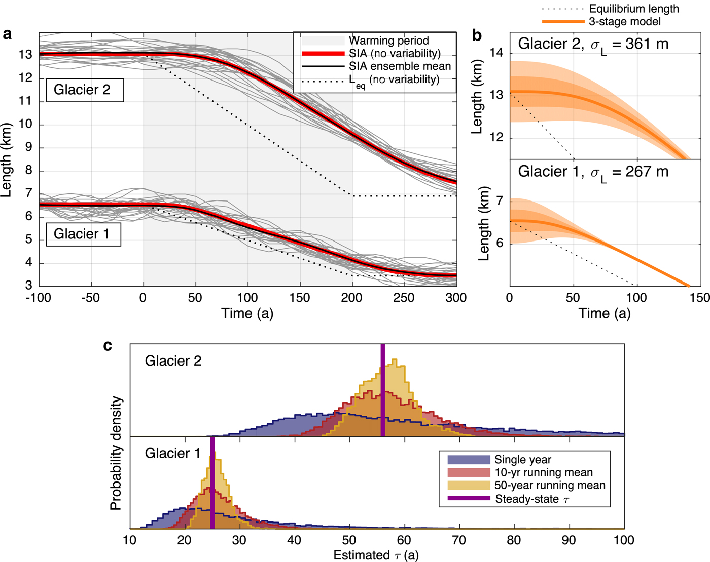
We now investigate our central question of the transient response to a climate trend. In the following analyses, we stipulate a linear trend in melt-season temperature of 2°C over 200 years, and no changes in precipitation, typical of the observed midlatitude trends over the last century (e.g., IPCC, Reference Stocker2013). Figure 3a shows the length responses of all four models and both geometries. All models exhibit a significant lag behind the equilibrium response (dashed line). However, the one-stage model's tendency to respond too quickly means that it underestimates the glacier's lag behind the changing climate. The good agreement among three-stage, SIA, and full-Stokes models suggests that the basic transient response to warming is not significantly affected by higher order ice dynamics, consistent with the conclusions of previous studies (e.g., Leysinger Vieli and Gudmundsson, Reference Leysinger Vieli and Gudmundsson2004).
The role of model complexity in response to a trend. (a) Length responses to a 2°C warming over 200 years, for all four models. The dashed lines show length at which the glaciers would be in equilibrium if the climate were to stabilize at that time. (b) Disequilibrium, defined as the difference between transient and equilibrium length, for glacier 2. (c) Fractional equilibration for glacier 2. (d) and (e) As for (b) and (c), but for glacier 1. The gray vertical line in each panel marks 140 years into the warming period as a reference point for current disequilibrium assuming anthropogenic forcing began ~1880.
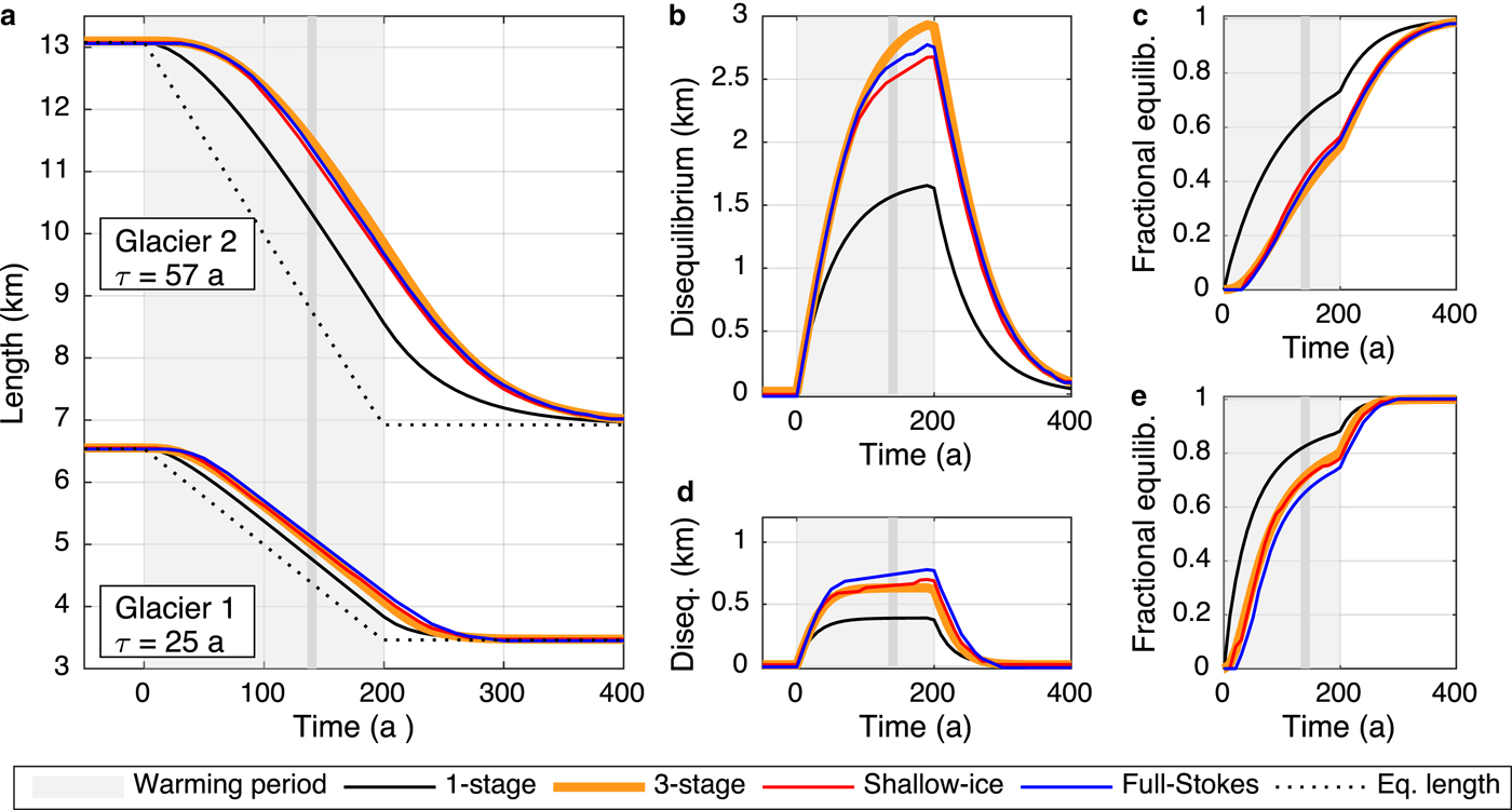
Figures 3b and c show the disequilibrium and fractional equilibration (as defined in Section 1.1), respectively, for glacier 2 (τ = 57 years), and Figures 3d and e show results for glacier 1 (τ = 25 years). The degree of disequilibrium is much more pronounced for the longer timescale glacier, consistent with its longer memory of previous, cooler climate states. It is important to note that the absolute length changes are greater for glacier 2 on account of its shallower bed slope. However, in terms of the fractional equilibration, we see that, by the end of the 200-year warming period, the three-stage, SIA, and full-Stokes models all show that the ‘slower’ glacier 2 has only worked through about half of its total adjustment to a 2°C warming; glacier 1 is about three-quarters of its way to equilibrium. The vertical lines in each panel mark 140 years into the warming as a rough comparison for the current state of glaciers, assuming anthropogenic forcing started ~1880 (e.g., IPCC, Reference Stocker2013). The basic physics of a lagged response to a trend implies that glaciers with long response times can be assumed to be significantly out of equilibrium with our current climate, both in an absolute and fractional sense.
3.2 Three different glaciers with the same response time
The marked difference in the responses of glaciers 1 and 2 to gradual warming shows the important role of the response time in setting the disequilibrium. Despite the simple form of the response time (Eqn (2)), a number of geometric, climatic, and rheological parameters are implicitly represented in the characteristic values H and b t. Given the range that these parameters may take for different glaciers around the world, it is important to consider the applicability of Eqn (2) across a range of parameter space. As an illustrative example, we present two additional idealized glaciers with different parameters for rheology, mass balance, and bed geometry. However, these parameters have been tuned in such a way to give response times (54 and 56 years) comparable with that of glacier 2 (57 years).
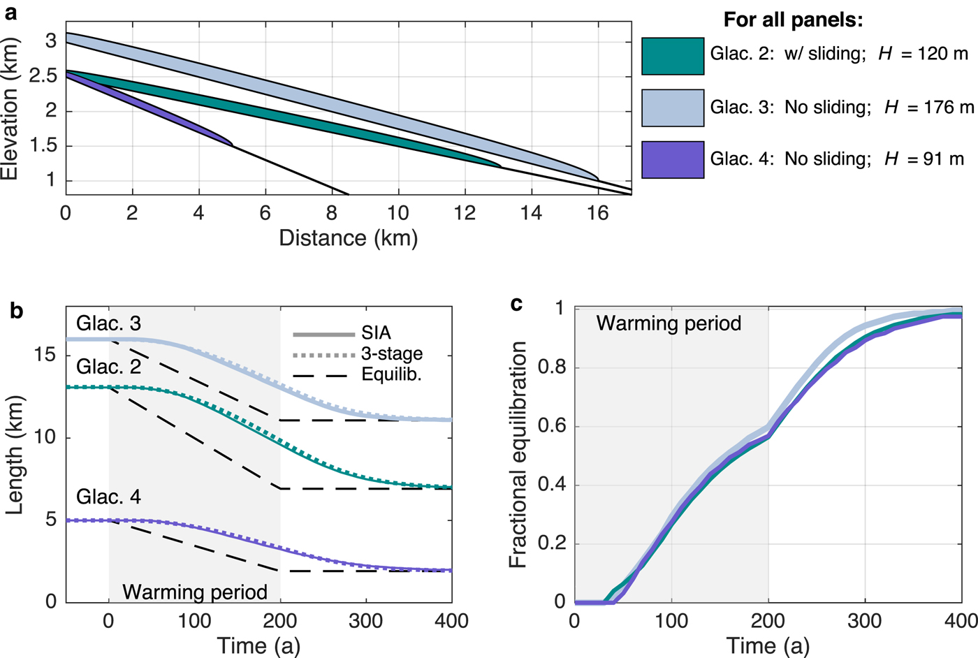
For simplicity, we only compare the SIA and three-stage models in this section. Table 2 displays the parameters and resulting geometries for glaciers 2–4, and SIA thickness profiles are shown in Figure 4a. Glacier 3 is slightly steeper than glacier 2, but does not slide over its bed, resulting in a greater steady-state mean ice thickness (176 m). Glacier 4 is steeper yet, and even with no sliding, has a mean thickness of only 91 m. Despite its smaller dimensions, it has a long response time because its terminus does not extend very far into lower, warmer elevations. All glaciers have the same accumulation rate of 4 m a−1 ice equivalent, but the maximum elevations and melt-season temperatures have been manipulated to give terminus positions, and thus mass-balance rates (b t), that yield the desired response times.
Three glaciers with ~55-year response timescales. (a) Initial equilibrium profiles for the three glaciers. Glacier 2 is the same as the larger glacier in the main text. Glaciers 3 and 4 do not have basal sliding. (b) Length responses of each glacier in response to a 2°C warming over 200 years. Solid lines are the SIA model response, dotted lines the three-stage model response, and black dashed lines show the instantaneous equilibrium lengths. (c) Fractional equilibration for each glacier (for clarity, only SIA responses are shown). Despite their different geometries and dynamics, the glaciers’ transient responses are nearly identical in a fractional sense.
Parameters and initial geometries for three glaciers with similar timescales. Results from the SIA model (bottom group) are inputs in the three-stage model
The three-stage model parameters are again based on the SIA equilibrium geometries. Figure 4b shows three-stage and SIA length responses to the same gradual warming (2°C over 200 years), which again agree closely. Owing to their different geometries, the length sensitivities (and thus equilibrium responses) are slightly different for the three glaciers. However, as Figure 4c shows, their responses are nearly identical in terms of fractional equilibration. Thus, we conclude that a glacier's fractional equilibration depends on its timescale (e.g, Figs 3c and e), but not on the glacier's length sensitivity (Fig. 4). This point is demonstrated analytically by the three-stage solution for fractional equilibration (Eqn (9)). Furthermore, that the three-stage model, which is blind to the details of sliding vs deformation, can emulate the SIA responses for each case suggests that glacier geometry encapsulates ice dynamics well enough to dictate the basic response to forcing. This makes τ – which is based on geometry and mass balance – a versatile metric for understanding glacier responses across a wide range of settings.
3.3. Uncertainty in response time
The essential lagged nature of the glacier response to a trend is robust across a range of geometries (Figs 3 and 4), but it depends on τ, and, via Eqn (2), ice thickness. In reality, ice thickness is often uncertain, and different estimation methods can yield different τ for the same glacier (e.g., Harrison and others, Reference Harrison, Elsberg, Echelmeyer and Krimmel2001; Oerlemans, Reference Oerlemans2001). So, we now evaluate how uncertainty in τ affects disequilibrium. The good agreement with the SIA and full-Stokes flowline models makes the three-stage model an efficient analytical tool. In the previous sections, we had the benefit of thickness profiles generated by the numerical models, and our results show that the mean ice thickness was an appropriate characteristic value to use in calculating τ. However, direct ice-thickness measurements on mountain glaciers are uncommon, and for more complex geometries, the mean may not be the best characteristic thickness for τ. Thus, we will use thickness in the following experiments to directly manipulate the response timescale.
We consider a broad uncertainty in thickness: a Gaussian probability distribution with a std dev. of  $\sigma _{\rm H} = \bar H/4$, where $\bar H$ is the mean thickness of the original flowline profiles that calibrated the three-stage model. This gives σ H = 13 m for glacier 1, and σ H = 31 m for glacier 2. With this value, the ± 2σ H range is equal to
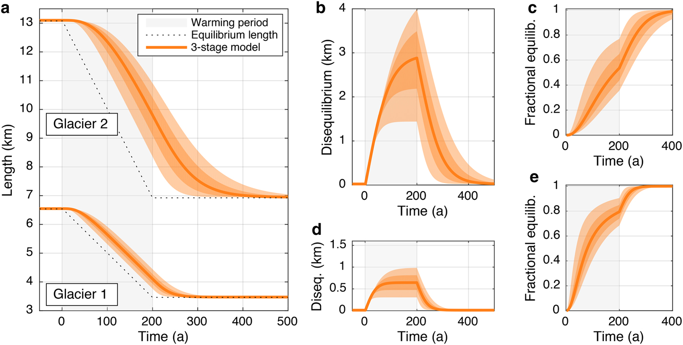
  $\bar H$ itself. Since τ is directly proportional to H, this yields a probability distribution for τ that also has the ± 2σ τ range equal to τ. Figure 5a shows the resulting length responses to our 2°C warming trend, with shaded regions showing the ± 1σ and ± 2σ bounds. The effect of timescale uncertainty is a sustained spread in length responses and, accordingly, in disequilibrium (Figs 5b and d) and fractional equilibration (Figs 5c and e). Errors in the response timescale introduce very long-term effects: the spread grows throughout the warming period, and persists well after the climate has re-stabilized. For instance, for glacier 2, the ± 1σ range in timescale (a spread of 28 years) yields a spread of ~1.3 km in length after 200 years of warming, or, to use the fractional metric, a range of ~60 years to reach 80% equilibration.
The spread of responses due to uncertainty in ice thickness. (a) Orange shaded regions show ± 1σ L and 2σ L bounds for uncertainty in timescale (σ τ = τ/4), generated with the three-stage model. The dashed line shows equilibrium length. (b, c) Associated spread in disequilibrium and fractional equilibration for glacier 2. (d, e) As for (b) and (c), but for glacier 1.
While ice thickness is a directly tunable parameter for the three-stage model, the effects of timescale uncertainty are also relevant to flowline modeling approaches where ice thickness depends in part on the rheological parameters and basal conditions. We used this dependence to tune flowline ice thicknesses in Section 3.2; similarly, Roe and Baker (Reference Roe and Baker2014) also showed that the response time (Eqn (2)) captures glacier response over a range of flowline model parameters. This suggests that errors in flowline model ice thickness, whatever their source, would cause errors in the length response similar to those in Figure 5.
3.4. Uncertainties due to climate variability
So far, we have considered the length response to a gradual warming in the framework of an idealized climate with no variations other than the imposed trend. In reality, however, any external climate forcing will occur in the midst of natural climate variability, which will continue to force low-frequency glacier length fluctuations (see Fig. 2c) on top of the retreat due to long-term warming. Figure 6a shows this behavior with an ensemble of length responses for different realizations of white-noise temperature and precipitation variability, σ T = 0.7 °C and σ P = 0.7 m a−1, superimposed upon the standard warming trend. The responses shown are 25 of 100 realizations generated using the SIA model, which was initialized from a steady-state configuration 200 years before the onset of warming in order to allow the fluctuations of each member to de-correlate. The three-stage model gives similar results, but is omitted for clarity. The fact that the ensemble mean is almost exactly equal to the trajectory for warming without variability reinforces that sustained disequilibrium is still the fundamental response in a noisy, warming climate. While variability may temporarily kick the glacier closer to its equilibrium length, it still has a restoring tendency back to the lagged state. We use a relatively high level of variability in these experiments to illustrate the potential uncertainties; it can be expected that a setting with less interannual variability would yield results more closely resembling the basic, lagged response.
Uncertainties due to climate variability. (a) An ensemble of length responses from the SIA model for a 2°C warming over 200 years, plus 100 realizations of white-noise variability (only 25 are shown). The ensemble mean (black) closely follows the length response to warming with no variability (red). The instantaneous equilibrium length for warming with no variability is plotted for reference (dashed line). (b) Uncertainty in initial state due to unknown climate history prior to the onset of warming (t = 0). Shaded regions show the ± 1σ L and 2σ L bounds for the same level of variability as in (a). Initial disequilibrium decays toward the long-term retreat trajectory. (c) Distributions of estimated timescale generated by tracking  $\bar H$ and b t through 10 000 years of noise-driven fluctuations. Blue is the distribution when sampling $\bar H$ and b t from a single year; red is the distribution for 10-year means; gold is the distribution for 50-year means; and the purple line shows the steady-state value.
These noise-driven fluctuations have several implications that must be considered for modeling the response of any glacier to climate warming. The possibility that the glacier was mid-fluctuation at the onset of the trend amounts to an uncertainty in initial conditions if the preceding climate is unknown. We illustrate this for the fluctuations driven by our standard interannual variability (σ T = 0.7 °C and σ P = 0.7 m a−1). Figure 6b shows the ± 1σ and ± 2σ bounds, where initial length anomalies are described by the Gaussian probability distributions with widths of σ L for each glacier. The impact of this uncertainty declines with time, on a timescale governed by τ. Initial-condition uncertainty does not therefore play a large role 140 years after the onset of the trend. While for the case considered here, the initial uncertainty arises from interannual climate variability, the same concept would apply to other poorly constrained climate histories. For example, accounting for little-ice-age excursions might entail a much larger uncertainty in initial conditions (e.g., Matthews and Briffa, Reference Matthews and Briffa2005).
Additional impacts of climate variability on glacier disequilibrium are the basic statistical challenges in defining the mean climate, trends, variability, and any parameters that rely on these estimates. The pre-trend climatology, equilibrium length, and the onset and magnitude of the climate trend are all uncertain quantities in a noisy climate; the accuracy of their estimates will vary depending on the level of climate variability and the length and quality of observational records. Estimates of the response timescale (τ = −H/b t) will also be affected by climate variability and the resulting glacier fluctuations. Even with observations, defining the characteristic values for ice thickness (here, the mean,  $\bar H$) and terminus ablation rates (b t) over decadal timescales may be uncertain due to sampling errors. Both $\bar H$ and the terminus elevation (and therefore b t) will vary with the glacier's low-frequency response to noise, but the dominant effect is simply the year-to-year variability in mass balance at the terminus. To investigate the effects on response-time estimates, we used the SIA model to track $\bar H$ and b t yearly through 10 000 years of climate noise for both glaciers (again, with σ T = 0.7 °C and σ P = 0.7 m a−1). From the $\bar H$ and b t timeseries, we calculated τ for each individual year. We then took running means of the $\bar H$ and b t timeseries to create distributions representing estimates of τ based on 10 and 50 years of observations. The probability densities for these distributions are shown in Figure 6c. Not surprisingly, a single year gives a poor estimate of τ, as shown by the broad, blue curves. The 10-year (red) and 50-year (gold) estimates converge on the steady-state values of τ = 25 and 57 years (vertical purple lines), but still have a substantial spread. While only the linear models require τ as an input parameter, this uncertainty is relevant for numerical flowline models as well. These sampling errors will still come to bear on the calibration of the glacier geometry, mass balance, and flow parameters, choices that must be made for any model, and which we have shown here fundamentally affect glacier response.
4. DISCUSSION
4.1. The committed retreat of mountain glaciers
The result that transient glacier retreat lags the equilibrium response to a climate trend stems fundamentally from the multi-decadal response times common to most mountain glaciers. Our focus on idealized glaciers, rather than specific settings, helps to demonstrate this basic behavior and the factors that affect it. Our comparison of several idealized geometries shows that a glacier's fractional equilibration during a climate trend depends strongly on its response time (glacier 1 vs 2 in Fig. 3), but not on its length sensitivity (glaciers 2–4 in Fig. 4). Figure 4 also shows that the fractional equilibration is the same for different parameter combinations that yield approximately the same value for τ = −H/b t. This makes τ a fundamental and useful parameter for categorizing glacier responses across a wide range of settings and geometries. Some general conclusions can thus be drawn about committed glacier retreat around the world based on estimated response times and observed climate trends (see, e.g., Roe and others, Reference Roe, Baker and Herla2017).
Consider that our synthetic 54–57-year glaciers are <50% into their adjustments to the total warming that has occurred in 140 years (see Fig. 4c). Given the observed global surface warming of ~1°C in the last century (e.g., IPCC, Reference Stocker2013), our results imply that longer timescale glaciers (τ>50 years) are substantially out of equilibrium today. In other words, their observed retreats are startling underestimates of the total retreat already built in by the industrial-era warming that has occurred to date. For large glaciers with shallow slopes and large length sensitivities, absolute disequilibrium may be on the order of kilometers (see Fig. 3b). This is consistent with several detailed modeling studies that have assessed committed retreat for large valley glaciers in the Alps. For example, Zekollari and others (Reference Zekollari, Fürst and Huybrechts2014) estimated the committed retreat of Morteratsch Glacier, based on 2001–10 climate, at nearly 2 km, while Jouvet and others (Reference Jouvet, Huss, Funk and Blatter2011) calculated a striking 6 km commitment for Great Aletsch Glacier based on 1989–2008 climate.
Additionally, while we have focused here on length changes, committed retreat also implies committed volume loss, which has direct implications for committed sea-level change (e.g., Mernild and others, Reference Mernild, Lipscomb, Bahr, Radić and Zemp2013; Marzeion and others, Reference Marzeion2017, Reference Marzeion, Kaser, Maussion and Champollion2018). While volume tends to react more quickly than length (e.g., Oerlemans, Reference Oerlemans2001), the committed loss should still depend on τ, making the distribution of individual response times an important consideration for regional or global estimates of committed volume change, and the associated impacts on sea level and hydrology.
Given some level of current disequilibrium, how certain is a glacier's committed retreat? For any component of the climate system, committed change is a useful metric because it is based on forcing that has occurred thus far, and is thus partitioned from changes associated with the much less certain future of anthropogenic forcing. However, a choice of definition must be made as to the way in which forcing is hypothetically stabilized. We have based committed retreat on an abrupt stabilization of temperature, as warming is a direct forcing on glacier extent (and is more robust than precipitation trends for most glaciers around the world; see, e.g., Roe and others, Reference Roe, Baker and Herla2017). However, the relevant forcing is different for other aspects of the climate system. Early studies on committed climate warming were based on a fixed atmospheric composition (e.g., Hansen and others, Reference Hansen1985; Wigley and Schlesinger, Reference Wigley and Schlesinger1985; Wigley, Reference Wigley2005), but this approach did not account for the finite lifetime of atmospheric greenhouse gases. As greenhouse gas emissions are the primary source of anthropogenic forcing (e.g., IPCC, Reference Stocker2013), more recent approaches calculate the climate commitment based on zero additional emissions. Although there is a broad spread of uncertainty, the central estimates are that if all anthropogenic emissions ceased today, the natural decline of greenhouse gases and the delayed ocean response would offset each other, leaving global temperatures approximately flat for the next few centuries (Solomon and others, Reference Solomon, Plattner, Knutti and Friedlingstein2009; Armour and Roe, Reference Armour and Roe2011; Mauritsen and Pincus, Reference Mauritsen and Pincus2017). These studies suggest that the observed warming to date constitutes a hard lower bound from which to calculate committed glacier retreat; and while calculating retreat based on current temperatures is an idealized approach, it is consistent with recent literature on committed change in the climate system.
4.2 Implications for climate reconstructions
The fact that glaciers lag their equilibrium response to a climate trend has important consequences for inferring past climates using numerical glacier models. A failure to account for current disequilibrium in the glacier state can render estimates of past climate significantly in error. Let dL/dT|eq be defined as the equilibrium sensitivity of a glacier to a change in mean temperature. For a glacier model, this is a fixed function of the parameters chosen by the modeler. In principle, one can use the model to infer the climate change required for a length change ΔL eq, between two equilibrium climate states. Assuming only changes in temperature, this can be written as:
 $${\rm \Delta} T_{{\rm eq}} = \; \displaystyle{{{\rm \Delta} L_{{\rm eq}}} \over {{\left. {{\rm d}L/{\rm d}T} \right \vert} _{{\rm eq}}}}.$$
However, because of the modern disequilibrium, an error is incurred if the modern length is used in calculating ΔL eq. For example, consider a moraine recording the glacier's equilibrium preindustrial extent, from which ΔL eq in Eqn (18) is set to L moraine − L modern. However, using glacier 2 as an example (τ = 57 years), the modern glacier has retreated less than halfway to its equilibrium length, so this assumed ΔL eq would underestimate the true equilibrium length change:
 $${\rm \Delta} L_{{\rm eq}} = (L_{{\rm moraine}} - L_{{\rm modern}}) \le \; \displaystyle{1 \over 2}\; \times \; \left. {{\rm \Delta} L_{{\rm eq}}} \right \vert ^{{\rm true}}.$$
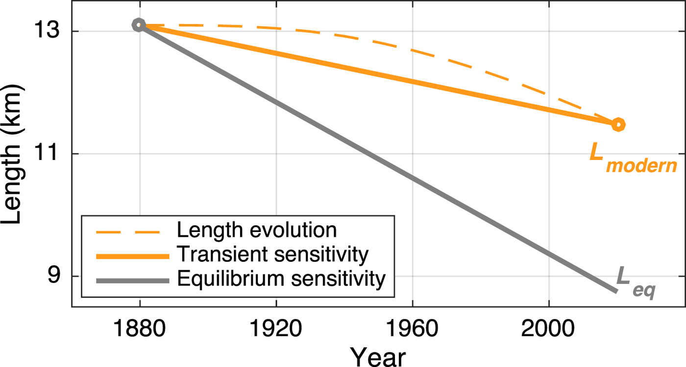
There are multiple possible consequences of the error. First, if the model sensitivity is correct, the resulting estimate of ΔT eq is less than half as large as the true climate change. The other possibility is that the glacier model parameters are tuned in a way that renders the model less than half as sensitive as it should be. This latter pitfall will occur when ΔT eq is constrained by instrumental or proxy records. Figure 7 illustrates this for glacier 2's response to a 1°C per century warming (dashed line), beginning in 1880. The average rate of retreat over the last 140 years (solid orange line) gives a transient sensitivity of −1.1 km°C−1, whereas the equilibrium sensitivity (gray line) is actually −2.9 km°C−1. A model tuned to the transient sensitivity would miscalculate any climate changes further in the past, and would also underestimate the natural glacier variability, σ L. Finally, some combination of errors in ΔT eq and the sensitivity is also possible. Whatever the case, it is clear that initializing a model in steady state with contemporary climate and length observations, when the target glacier is in fact far out of equilibrium, means building significant error into any analyses that rely on the model.
A number of approaches for reconstructing climate from glacier records exist (see, e.g., a review by Mackintosh and others, Reference Mackintosh, Anderson and Pierrehumbert2017 and references therein). However, the effects of disequilibrium have not been emphasized in the reconstruction literature. The consequences of ignoring current disequilibrium would vary by methodology and by glacier, but our results suggest that disequilibrium should be factored into any length sensitivity estimates or model calibrations based on current geometry. Errors would be particularly problematic for estimates of late-Holocene climate changes relative to the modern climate, and for glaciers with long response times. They become less of an issue for larger glacier changes, such as retreat from the Last Glacial Maximum, where the modern disequilibrium is a smaller fraction of the overall change; or, for glaciers with fast response times, whose current state is closer to equilibrium.
Transient vs equilibrium sensitivity. The dashed orange line shows the three-stage length response of glacier 2 to the 1°C century−1 warming, beginning in 1880. Transient length sensitivity inferred from terminus retreat (solid orange line) underestimates the glacier's equilibrium sensitivity (gray line). The transient sensitivity is −1.1 km°C−1, while the true equilibrium sensitivity is −2.9 km°C−1.
4.3. Implications for glacier projections
Modeling glacier retreat is also a vital part of predicting and adapting to impacts of glacier change in a warming climate, such as sea-level and hydrological changes (e.g., IPCC, Reference Stocker2013). Uncertain emissions scenarios and regional climate variability introduce a large amount of uncertainty into localized projections (e.g., Deser and others, Reference Deser, Phillips, Alexander and Smoliak2014), but because the metric of committed retreat is independent of future forcing by construction, it can provide a useful bound for assessing future impacts. Current disequilibrium is also important to assess because the model sensitivity issues discussed above also apply to projections of future retreat: whatever the future forcing scenario, initializing glacier models in steady state with the current climate will introduce errors into the predicted retreat and the glacier's contributions to catchment hydrology.
Another point related to future glacier change is that over the initial period of gradual warming (i.e., up to a few multiples of τ), terminus retreat accelerates even as the rate of warming remains steady. This acceleration can be conceptualized in the three-stage framework of Roe and Baker (Reference Roe and Baker2014): melt-driven thinning reduces flux into the terminus region, eventually making ablation more efficient at driving terminus retreat. This sequence is more drawn out for longer response timescales, and our results suggest that glaciers with 50+ year response times have not emerged from this early stage of adjustment to anthropogenic warming. In other words, their recent responses may be characterized more by thinning than by terminus retreat. Indeed, dramatic thinning has been observed for many mountain glaciers (see, e.g., Paul and others, Reference Paul, Kääb, Maisch, Kellenberger and Haeberli2004), and may be a precursor to increased retreat for long-timescale glaciers. These stages of response should thus be considered when interpreting recent or future changes in retreat rates.
4.4 The role of higher order ice dynamics
In addition to considering model tuning and initialization, the representation of ice dynamics is also an important decision that the modeler faces, and the degree of complexity required ultimately depends on the question being asked: shallow-ice solutions can give errors in the spatial pattern of ice thickness or velocities (e.g., Le Meur and others, Reference Le Meur, Gagliardini, Zwinger and Ruokolainen2004; Greve and Blatter, Reference Greve and Blatter2009; Adhikari and Marshall, Reference Adhikari and Marshall2011, Reference Adhikari and Marshall2013); however, Adhikari and Marshall (Reference Adhikari and Marshall2013) also showed that the discrepancies between higher and lower order solutions were greater for advance scenarios than for retreat. Leysinger Vieli and Gudmundsson (Reference Leysinger Vieli and Gudmundsson2004) compared full-Stokes and SIA model responses to step changes in climate, making the important point that accurate mass-balance information may be more critical than higher order dynamics for modeling glacier responses to climate changes. The close agreement between our SIA and full-Stokes simulations indicate that higher order stresses do not play a large role in the basic, lagged response to gradual warming, consistent with the insights of Leysinger Vieli and Gudmundsson (Reference Leysinger Vieli and Gudmundsson2004) and Adhikari and Marshall (Reference Adhikari and Marshall2013). We find that accurate ice thickness and mass balance, which robustly characterize the response time, are more important than model complexity for representing disequilibrium, provided that three-stage (as opposed to one-stage) dynamics are used if a linear model is chosen (see also discussion in Roe and Baker, Reference Roe and Baker2014). However, a uniform bed geometry and absence of lateral effects make it more likely that SIA (and three-stage) assumptions hold. Several studies have shown that the choice of model dynamics may affect the steady-state thickness distribution (e.g., Le Meur and others, Reference Le Meur, Gagliardini, Zwinger and Ruokolainen2004; Adhikari and Marshall, Reference Adhikari and Marshall2013). Thus, for modeling experiments that target specific glacier geometries, the inclusion of higher order stresses may become important for representing the degree of disequilibrium through the response time, even if higher order mechanics do not play a major role in retreat.
4.5. Outlook
Estimates of past climate change and predictions of future glacier retreat must take the current disequilibrium of glaciers into account. However, without perfect knowledge of the system, there is an unavoidable quandary here: current climate is typically well observed, but current disequilibrium may be uncertain because the response time can only be estimated approximately (e.g., Fig. 5). On the other hand, while the disequilibrium was less (though not necessarily absent) at the start of the industrial era, the climate then may be less certain. Nevertheless, records of glacier front position at the beginning of the industrial era are abundant (e.g., Leclercq and others, Reference Leclercq2014), and several global datasets of temperature extend back to 1880 (e.g., Rhode and others, Reference Rohde2013). Our opinion is that in many parts of the world, sufficient climate and glacier data exist to incorporate disequilibrium into interpretations of glacier change and model initialization. One approach is a dynamic calibration, using a model of at least three-stage complexity, to account for transient effects and identify glacier and climate parameters (e.g., Table 1) together with their uncertainties that best reproduce the observed retreat. Such a calibrated model could then be used to estimate older climate changes or future glacier responses. Dynamic calibration has been applied to a number of well-observed glaciers (e.g., Oerlemans, Reference Oerlemans1997; Lüthi and others, Reference Lüthi, Bauder and Funk2010; Jouvet and others, Reference Jouvet, Huss, Funk and Blatter2011; Zekollari and others, Reference Zekollari, Fürst and Huybrechts2014). Additionally, Roe and others (Reference Roe, Baker and Herla2017) applied this approach, using the three-stage model, to compare natural glacier variability with observed retreats around the world. In any event, it is vital to produce reconstructions and projections that reflect uncertainties in model parameters. Because each glacier setting is unique, modeling efforts are often targeted to a single glacier, and it is easy for calibration choices to be made that affect the model sensitivity. As the results of this paper demonstrate, the errors can be severe when modern glaciers are assumed to be near equilibrium.
5. SUMMARY AND CONCLUSIONS
Because many mountain glaciers have response timescales that are similar in order to the period of time over which humans have been changing the climate, we should not assume that they are close to equilibrium in response to this forcing (see Fig. 1). We explored the factors that influence this disequilibrium and that modelers must take into account to properly capture the transient response. Specifically, we considered (a) the representation of ice dynamics; (b) the glacier's geometry, and therefore its response timescale; and (c) the effects of climate variability on model initialization and glacier response. Our main findings in these areas are summarized as follows:
(a) A comparison of four models of ice dynamics forced by the same ramp warming showed that, at a minimum, three-stage linear dynamics were necessary to accurately capture a glacier's degree of disequilibrium. The one-stage linear model captures the basic phenomenon of disequilibrium, but underestimates its magnitude by about a factor of two in our results; this is because it too-rapidly translates mass-balance perturbations into length changes. A number of other low-order glacier models exist in the literature; our comparisons indicate that accurately capturing the lag between forcing and terminus response (or equivalently, the phase lag in the cross spectrum; Roe and Baker, Reference Roe and Baker2014), as the three-stage does, is a prerequisite for any analytical model used to estimate disequilibrium. The three-stage model emulates the response of the flowline models very well, despite its dependence on fixed parameters linearized about a mean state. Roe and Baker (Reference Roe and Baker2014) showed that the three-stage parameters could be calibrated for more complex valley geometries, and could still reasonably emulate flowline model output for terminus fluctuations. However, they noted greater disagreement for large excursions that spanned slope breaks in the glacier bed. It can be expected that linear-response models will become less accurate when modeling a retreat that traverses significant changes in the valley geometry. Thus, while the three-stage model succeeded here in modeling time-varying glacier retreat, more complex geometries may call for at least SIA or higher order flowline models.
(b) In contrast to the close agreement of three-stage and flowline model outputs, the distribution of responses associated with uncertainty in ice thickness, and thus timescale, is quite broad (Fig. 5). This is ultimately a simple result – adjusting the timescale, by construction, adjusts how quickly the glacier can respond to a climate change, and thus how much it lags a trend. However, because this lag is unyielding, errors related to the response timescale are persistent, and necessarily bear upon estimates of current disequilibrium and projections of future retreat.
(c) Random, interannual climate variability introduces several complications when modeling transient glacier retreat. Terminus fluctuations due to a noisy mass-balance history imply an uncertainty in initial conditions, but the effects of an initial length perturbation decay and are of negligible significance after a few multiples of τ. However, a noisy climate can also have persistent impacts on modeled glacier responses, because mass-balance variability and glacier fluctuations mean that estimates of glacier parameters are subject to sampling errors. Even with multi-decade running means, substantial year-to-year variability can mean non-trivial uncertainty in the mean value of τ (Fig. 6c), and thus the degree of disequilibrium. Finally, length responses to an ensemble of noisy, warming climates demonstrate that, while climate variability can cause glacier retreat to slow or even reverse for a short period, the terminus does indeed fluctuate around its lagged, not equilibrium, trajectory (Fig. 6a). So, while climate variability inevitably clouds our metrics for quantifying it, glacier disequilibrium should be considered a robust phenomenon in the global aggregate, and as the warming trend continues.
While individual glacier dynamics can be quite complicated, a simple lesson from our work is clear: mountain glaciers with multi-decadal response times are among the many components of the climate system whose modern state is one of both realized and committed change. We have already witnessed significant glacier retreat over the past century, but the disequilibrium of these systems with the modern climate means that responses to continued climate warming are inextricably compounded by ongoing adjustment to the warming of the past decades. However, if estimates of the glacier timescale, length sensitivity, and the warming trend are available, current disequilibrium can be accounted for when calibrating models and interpreting observations. The basic behavior and dependencies discussed here can provide a framework for refining reconstructions of past climate, estimates of current glacier state, and projections of future glacier retreat.
ACKNOWLEDGEMENTS
We thank three anonymous reviewers for thorough and thoughtful comments that helped us clarify the manuscript. We are also grateful to Benjamin Smith (Applied Physics Laboratory, U. Washington) for assistance with and access to modeling resources; and to the scientific editor, Ralf Greve, for helpful comments and effective handling of the manuscript. J.E.C. was supported by the National Science Foundation Graduate Research Fellowship Program (DGE-1256082).


 Open access