1. Introduction
Running a cosmological simulation, whether N-body or full hydrodynamical, is the first step in understanding cosmic structure formation and the evolution of galaxies. A critical step in extracting information from sophisticated, multi-billion particle simulations is the identification of structures, like dark matter (DM) halos and synthetic galaxies. Identifying (sub)structures is a non-trivial task and has led to the development of equally sophisticated structure finders (see Knebe et al. Reference Knebe2011; Onions et al. Reference Onions2012; Knebe et al. Reference Knebe2013a, Reference Knebe2013b, for an overview of (sub)halo/galaxy finding). A variety of codes exist that attempt to excise structures of interest from simulations, with most focusing on searching for overdense, gravitationally self-bound regions within cosmological simulations. For cosmological N-body simulations, these objects are DM halos, and for hydrodynamical simulations, these objects can be galaxies.
The two most common pure halo finders are Friends-of-Friends (FOF) algorithms (e.g. Davis et al. Reference Davis, Efstathiou, Frenk and White1985) and Spherical Overdensity algorithms (e.g. Lacey & Cole Reference Lacey and Cole1994), the former using a linking length based on a desired density criterion, and the latter identifying density peaks and grouping all particles within a spherical region that encloses some density (see Knebe et al. Reference Knebe2011, for a more thorough discussion and comparison of halo finding).
Beyond halo finders are those that also attempted to excise substructures residing within the gravitationally collapsed, nonlinear environment of halos, the so-called subhalo finders. Subhalo finders can be broadly classified into two types: configuration-space finders and phase-space finders. Older, more common configuration-space finders, like ahf (Knollmann & Knebe Reference Knollmann and Knebe2009), subfind (Springel et al. Reference Springel, White, Tormen and Kauffmann2001), and adaptahop (Tweed et al. Reference Tweed, Devriendt, Blaizot, Colombi and Slyz2009), search for physical overdensities or clustering in configuration space.Footnote a Phase-space finders, like hsf (Maciejewski et al. Reference Maciejewski, Colombi, Springel, Alard and Bouchet2009) and rockstar (Behroozi, Wechsler, & Wu Reference Behroozi, Wechsler and Wu2013), use extra velocity information to identify overdensities and clustering in the full phase space.
Different (sub)halo finders suffer from different issues (see Knebe et al. Reference Knebe2013b, for a in depth discussion of structure finding). Configuration-space-based finders rely on saddle points in the density field in some form or another to separate structures. Consequently, subhalos are artificially truncated as they fall towards pericentre and grow again as the move out to apocentre (see Muldrew, Pearce, & Power Reference Muldrew, Pearce and Power2011; Behroozi et al. Reference Behroozi2015, for specific examples using subfind & ahf). Phase-space finders are better able to separate these structures since they will overlap less in phase space, and in principle need not inherently shrink/grow the mass associated with subhalos as they move towards pericentre/apocentre.
Here we present VELOCIraptor (formerly known as STructure Finder, stf; Elahi, Thacker, & Widrow Reference Elahi, Thacker and Widrow2011), a phase-space (sub)halo finder capable of identifying DM halos and galaxies.Footnote b This code can ingest both pure N-body simulation input and hydrodynamical data. Here we present significant update to the original algorithm described in Elahi et al. (Reference Elahi, Thacker and Widrow2011).
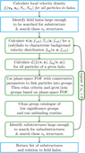
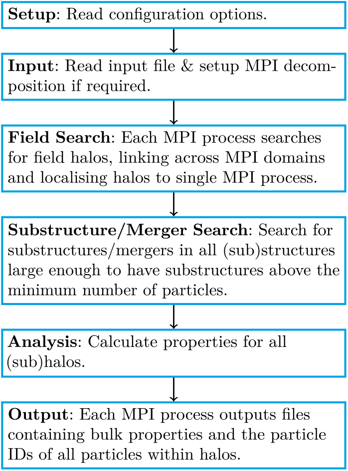
Activity chart of VELOCIraptor.
Our paper is organised as follows: in Section 2 we outline the code package, present tests of our algorithm in Section 3, and conclude in Section 4 with a summary and discussion.
2. Identifying structures with VELOCIraptor
VELOCIraptor is a (sub)halo finder that identifies structures in a multi-stage process, the exact details depending on the operational mode it is being used in: identifying DM halos, DM halos+baryonic content, or just galaxies. VELOCIraptor is built on stf (Elahi et al. Reference Elahi, Thacker and Widrow2011), providing significant upgrades to the halo finding algorithm, treatment of baryons, the mass reconstruction of major merger events, along with parallelisation and integration into N-body codes (specifically swift; Schaller et al. Reference Schaller, Gonnet, Chalk and Draper2016). We describe the various aspects of our code below. For readers interested in input interfaces, output, and general modes of operation, we suggest skipping to Section 2.6. Readers interested in the main benefits and results of VELOCIraptor can skip to Section 3.
The identification process proceeds in a two-stage approach: (1) identify field halos/galaxies; and (2) for each field object search for substructure using phase-space information. Unlike almost all other structure finders currently available, this algorithm is also capable of robustly identifying tidally disrupted objects (see Elahi et al. Reference Elahi2013) along with self-bound, physically dense halos/galaxies. A flow chart describing the operational stages is shown in Figure 1.
2.1. Field halos
The code first identifies candidate halos using a 3DFOF algorithm (3D Friends-of-Friends in configuration space, see Davis et al. Reference Davis, Efstathiou, Frenk and White1985), linking particles together if
 $$\matrix{
{{{{{\left( {{{\rm{x}}_i} - {{\rm{x}}_j}} \right)}^2}} \over {\ell _{\rm{x}}^2}} \lt 1,}} $$
$$\matrix{
{{{{{\left( {{{\rm{x}}_i} - {{\rm{x}}_j}} \right)}^2}} \over {\ell _{\rm{x}}^2}} \lt 1,}} $$
where xi is the ith particle’s position, and ℓ x is the linking length. This initial linking can also make use of a particle’s type, whether DM (N-body), or gas, star (baryon). Cosmological simulations typically set ℓ x = 0.2 times the inter-particle spacing.
Simple FOF algorithms are susceptible to artificially joining two structures together by a single (or a few) particle(s), a so-called particle bridge. We appeal to the physics of the structures we seek to identify, i.e., virialised halos, and use velocity information.Footnote c For each structure k we calculate a velocity dispersion, σ v,k, and apply a 6DFOF,
 $$^{\matrix{{{{{{\left( {{x_i} - {x_j}} \right)}^2}} \over {\ell _x^2}} + {{{{\left( {{v_i} - {v_j}} \right)}^2}} \over {\ell _v^2}} \lt 1,}} }$$
which splits virialised structures connected by dynamically unrelated particle bridges and tends to remove very unbound particles that may have been grouped by the original FOF algorithm. Here ℓ v = α vσ v,k, and α v is a scaling term on the order of unity.
Addition of baryons: Simulations can contain both N-body (DM) particles and other particle types and along with the inclusion of extra forces, like the addition of gas tracers and hydrodynamical forces. Fully hydrodynamical cosmological simulations often contain gas particles (or tracers for codes such as AREPO; Springel Reference Springel2010, or cells such as ramses; Teyssier Reference Teyssier2002), star particles, and even sink particles representing supermassive black holes. These baryons tracers can be treated in a special fashion by VELOCIraptor if the appropriate flags are set. If desired, specific particle types can be searched, such as stars to produce a galaxy catalogue. The code can also search all particle types, either treating all particles equally or allowing for special linking behaviour dependent on particle type.
The two most common modes of operation are either to assign baryonic particles to DM structures, the so-called DM+Baryons, or to search only star particles and identify galaxies, the so-called Galaxies+Baryons. We discuss how the field search operates in both these modes.
Since gas particles are subject to hydrodynamical forces and can clump together to form long filaments, applying a simple FOF algorithm can lead to the artificial linking together of several dynamically distinct structures. Hence the typical mode of operation to group both DM and baryons together is to produce FOF links using DM particles only, i.e., a DM particle can link to other DM particles and baryon particles, but baryon particles are ignored when searching for new FOF links. An application of this mode has been applied to hydrodynamical zoom simulations (e.g. Elahi et al. Reference Elahi2016; Arthur et al. Reference Arthur2017).
When searching for galaxies using star particles, we first identify 3DFOF stellar structures. These structures are then searched using a 6DFOF, with the critical difference between the DM search being that we keep track of the star particles linked in the 3DFOF but not linked in the 6DFOF as a structure. This remnant 3DFOF represents the diffuse, kinematically distinct stellar halos that surround galaxies. An application of this mode has been applied to hydrodynamical simulations to look at the sizes of galaxies and a preliminary investigation of diffuse stellar halos (Cañas et al. Reference Cañas, Elahi, Welker, Lagos, Power, Dubois and Pichon2018, Canas et al., in preparation). The code can also use star particles as a basis for links to assign other baryonic particle types to structures in a similar fashion to the DM mode described above.
Activity chart for identifying substructures.
2.2. Subhalos and streams
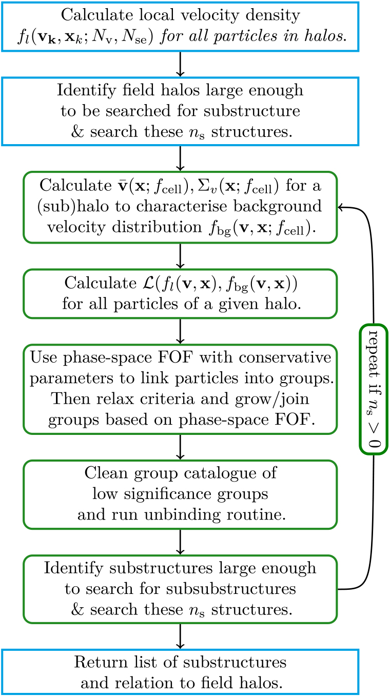
We briefly describe the specifics of identifying substructures here as it is discussed in Elahi et al. (Reference Elahi, Thacker and Widrow2011). Substructures are identified using a phase-space FOF algorithm on particles that appear to be dynamically distinct from the mean ‘Maxwellian’ halo background, i.e., particles which have a local velocity distribution that differs significantly from the mean, smooth background halo. This approach is capable of finding not only subhalos, but also tidal debris surrounding subhalos as well as tidal streams from completely disrupted subhalos. The method for identifying substructure is shown in Figure 2.
Dynamically distinct particles: The algorithm identifies particles that are dynamically distinct from a background distribution by examining velocity space assuming that a halo’s velocity distribution can be split into a virialised background and substructures.
To illustrate this method, consider the phase-space distribution function:
 $$\matrix{
{F\left( {{\rm{x}},{\rm{v}}} \right) = \rho \left( {\rm{x}} \right)f\left( {\rm{v}} \right)}} $$
$$\matrix{
{F\left( {{\rm{x}},{\rm{v}}} \right) = \rho \left( {\rm{x}} \right)f\left( {\rm{v}} \right)}} $$
Here we assume the distribution function is separable into ρ(x) and f (v), the physical and velocity density distribution functions, respectively. Assuming Gaussian velocity distributions for a substructure and a halo, the distribution ratio of a substructure S to the background bg at a given (x, v) is:
 $$\matrix{
{{{{F_{\rm{S}}}\left( {{\rm{x}},{\rm{v}}} \right)} \over {{F_{{\rm{bg}}}}\left( {{\rm{x}},{\rm{v}}} \right)}} = [{{\rho {\rm{S}}\left( {\rm{X}} \right)} \over {{\rho _{{\rm{bg}}}}\left( {\rm{X}} \right)}}][{{\sigma _{{\rm{bg}}}^3} \over {\sigma _{\rm{S}}^3}}][{{{{\rm{e}}^{ - \left( {{\rm{v - }}{{\rm{v}}_{\rm{s}}}} \right)}}^2/2\sigma _{\rm{S}}^2} \over {{{\rm{e}}^{ - \left( {{\rm{v - }}{{\rm{v}}_{{\rm{bg}}}}} \right)}}^2/2\sigma _{{\rm{bg}}}^2}}].}} $$
$$\matrix{
{{{{F_{\rm{S}}}\left( {{\rm{x}},{\rm{v}}} \right)} \over {{F_{{\rm{bg}}}}\left( {{\rm{x}},{\rm{v}}} \right)}} = [{{\rho {\rm{S}}\left( {\rm{X}} \right)} \over {{\rho _{{\rm{bg}}}}\left( {\rm{X}} \right)}}][{{\sigma _{{\rm{bg}}}^3} \over {\sigma _{\rm{S}}^3}}][{{{{\rm{e}}^{ - \left( {{\rm{v - }}{{\rm{v}}_{\rm{s}}}} \right)}}^2/2\sigma _{\rm{S}}^2} \over {{{\rm{e}}^{ - \left( {{\rm{v - }}{{\rm{v}}_{{\rm{bg}}}}} \right)}}^2/2\sigma _{{\rm{bg}}}^2}}].}} $$
This ratio has three terms: the physical density contrast; velocity dispersion contrast; and a ratio of Gaussian terms. Subhalos are dynamically cold overdensities, unlike tidal streams, which can have negligible density contrasts and velocity dispersion comparable with the background. Hence, it is a common practice to focus on the density ratio to identify subhalos. However, regardless of whether a substructure is a subhalo or tidal debris, the velocity distribution of the particles belonging to the substructure will differ from the background. These particles will have a ratio of at least exp  $ \left( {\delta {v^2}/2\sigma _{{\rm{bg}}}^2} \right)$.
This exponential factor, a measure of orbit clustering, is key to our algorithm. Instead of estimating the full phase-space density at a particle’s phase-space position X, wemeasure local velocity density, f l(v|x), as this is less computationally expense and not as noisy. We then divide out the expected velocity density of the background, f bg(v|x), neglecting the first term in Equation (4) at this stage. Particles belonging to velocity distributions that differ from the background will have ratios of f l/ f bg ≫ 1.
The local velocity density of a particle k, f l(vk), is measured using a kernel-scheme with an Epanechnikov smoothing kernel (Sharma & Steinmetz Reference Sharma and Steinmetz2006). This density is calculated using N v nearest velocity neighbours from the set of N se nearest physical neighbours, where N v < N se.Footnote d Typical values are N v = 32, N se = 256.
The mean background velocity density is characterised by a multivariate Gaussian,Footnote e thus, the expected background velocity density for a particle k with velocity vk is
 $$\matrix{
{{f_{{\rm{bg}}}}\left( {{{\rm{v}}_k}} \right) = {{{\rm{exp[ - }}{1 \over 2}\left( {{{\rm{v}}_k} - \overline {\rm{v}} \left( {{{\rm{x}}_k}} \right)} \right)\Sigma _v^{ - 1}\left( {{{\rm{x}}_k}} \right)\left( {{v_k} - \overline {\rm{v}} \left( {{{\rm{x}}_k}} \right)} \right){\rm{]}}} \over {{{\left( {2\pi } \right)}^{3/2}}|{\Sigma _v}\left( {{{\rm{x}}_k}} \right){|^{1/2}}}},}} $$
$$\matrix{
{{f_{{\rm{bg}}}}\left( {{{\rm{v}}_k}} \right) = {{{\rm{exp[ - }}{1 \over 2}\left( {{{\rm{v}}_k} - \overline {\rm{v}} \left( {{{\rm{x}}_k}} \right)} \right)\Sigma _v^{ - 1}\left( {{{\rm{x}}_k}} \right)\left( {{v_k} - \overline {\rm{v}} \left( {{{\rm{x}}_k}} \right)} \right){\rm{]}}} \over {{{\left( {2\pi } \right)}^{3/2}}|{\Sigma _v}\left( {{{\rm{x}}_k}} \right){|^{1/2}}}},}} $$
where  $ \overline {\rm{v}} $ is the mean velocity, and σv is the matrix representation of velocity dispersion tensor about $\overline {\rm{v}} $
 , both of which depend on the position within the halo, x.
The mean field is estimated by splitting the halo into volumes containing enough particles so that the statistical error on bulk quantities calculated for a cell is negligible but not so large that density (and thus the velocity dispersion) varies greatly across the volume. To balance these competing effects, we split the halo into cells containing N cell particles using a KD-Tree (Friedman, Bentley, & Finkel Reference Friedman, Bentley and Finkel1977; Appel Reference Appel1985; Barnes & Hut Reference Barnes and Hut1986), iteratively splitting along the spatial dimension that maximises Shannon entropy, S. We calculate S for each dimension by binning particles in n bins that span the extent of the dimension using the formula
 $$\matrix{
{S = {1 \over {\log {n_{{\rm{bins}}}}}}\sum\limits_k^{{n_{{\rm{bins}}}}} - {{{m_k}} \over {{m_{{\rm{tot}}}}}}{\rm{log}}{{{m_k}} \over {{m_{{\rm{tot}}}}}},}} $$
$$\matrix{
{S = {1 \over {\log {n_{{\rm{bins}}}}}}\sum\limits_k^{{n_{{\rm{bins}}}}} - {{{m_k}} \over {{m_{{\rm{tot}}}}}}{\rm{log}}{{{m_k}} \over {{m_{{\rm{tot}}}}}},}} $$
where m k is the mass in the kth bin and m tot is the total mass. This process splits volumes in the dimension with the greatest amount of variation in the spacing between particles, effectively minimises the variation in particle density across any given cell volume.
The cell size sets the background scale, below which we can robustly identify orbital clustering. We typically set N cell = f cellN H, where f cell ∼ 0.01 is the fraction of N H, the number of particles in the halo. This fraction is increased if N cell ≳ 100 up to a maximum of ∼ 1/8N H in order to have an accurate dispersion tensor.
For each volume we calculate the centre-of-mass, centre-of-mass velocity, and the velocity dispersion tensor:
 $$\matrix{
{\overline {\rm{x}} = {1 \over {{M_{{\rm{cell}}}}}}\mathop \Sigma \limits_k {m_k}{{\rm{x}}_k},}} $$
$$\matrix{
{\overline {\rm{v}} = {1 \over {{M_{{\rm{cell}}}}}}\mathop \Sigma \limits_k {m_k}{{\rm{v}}_k},}} $$
$$\matrix{
{\overline {\rm{x}} = {1 \over {{M_{{\rm{cell}}}}}}\mathop \Sigma \limits_k {m_k}{{\rm{x}}_k},}} $$
$$\matrix{
{\overline {\rm{v}} = {1 \over {{M_{{\rm{cell}}}}}}\mathop \Sigma \limits_k {m_k}{{\rm{v}}_k},}} $$
 $$\matrix{
{\sigma _{i,j}^2 = {1 \over {{M_{{\rm{cell}}}}}}\mathop \Sigma \limits_k {m_k}\left( {{v_{k,i}} - \overline {{v_i}} } \right)\left( {{v_{k,j}} - \overline {{v_j}} } \right),}} $$
$$\matrix{
{\sigma _{i,j}^2 = {1 \over {{M_{{\rm{cell}}}}}}\mathop \Sigma \limits_k {m_k}\left( {{v_{k,i}} - \overline {{v_i}} } \right)\left( {{v_{k,j}} - \overline {{v_j}} } \right),}} $$
where M cell is the mass contain in the cell and the sums are over all particles in the cell. The velocity quantities are interpolated to a particle’s position with an inverse-distance interpolation scheme using the cell containing the particle and the six neighbouring cells (those that share faces with the cell of interest):
 $$\matrix{
{u\left( {\rm{x}} \right) = \mathop \Sigma \limits_{i = 0}^N {{{w_i}\left( {\rm{x}} \right){u_i}} \over {\Sigma _{j = 0}^N{w_j}\left( {\rm{x}} \right)}},}} $$
$$\matrix{
{u\left( {\rm{x}} \right) = \mathop \Sigma \limits_{i = 0}^N {{{w_i}\left( {\rm{x}} \right){u_i}} \over {\Sigma _{j = 0}^N{w_j}\left( {\rm{x}} \right)}},}} $$
where u is the quantity we wish to determine at a position x based on cells with centre-of-mass positions  $ {\overline {\rm{x}} _i}$, and ${w_i}\left( {\rm{x}} \right) = |x - {\overline {\rm{x}} _i}{|^{ - 1}} $
 .
.
We then calculate the logarithmic ratio for each particle k,
 $$\matrix{
{{\mathcal{ R}_k} = {\rm{ln[}}{f_1}\left( {{{\rm{v}}_k}|{{\rm{x}}_k}} \right){\rm{/}}{f_{{\rm{bg}}}}\left( {{{\rm{v}}_k}|{{\rm{x}}_k}} \right){\rm{]}}{\rm{.}}}} $$
$$\matrix{
{{\mathcal{ R}_k} = {\rm{ln[}}{f_1}\left( {{{\rm{v}}_k}|{{\rm{x}}_k}} \right){\rm{/}}{f_{{\rm{bg}}}}\left( {{{\rm{v}}_k}|{{\rm{x}}_k}} \right){\rm{]}}{\rm{.}}}} $$
As both quantities have noise, this noise must be taken into account to determine if a particle is an outlier of the background distribution and belongs to a substructure. Based on tests using smooth, spherical halos with density profiles ranging from cored isothermal to a steep r −1.5(1 + r/a o)−1.5 generated by galactICS (Kuijken & Dubinski Reference Kuijken and Dubinski1995; Widrow & Dubinski Reference Widrow and Dubinski2005; Widrow, Pym, & Dubinski Reference Widrow, Pym and Dubinski2008), the  $\mathcal{R}$-distribution is characterised by Skew-Gaussian:
 $$\matrix{
{\mathop {{f_{{\rm{SG}}}}\left( {\mathcal{ R};\mathcal{\overline R} ,{\sigma _\mathcal{ R}},s,A} \right) = A\{ {\rm{exp [}} - {{{{\left( {\mathcal{ R} - \mathcal{\overline R} } \right)}^2}} \over {2{s^2}\sigma _\mathcal{ R}^2}}{\rm{]}}\theta \left( {\mathcal{\overline R} - \mathcal{ R}} \right)}\limits_{\matrix{
{ + {\rm{exp[}} - {{{{\left( {\mathcal{ R} - \mathcal{\overline R} } \right)}^2}} \over {2\sigma _\mathcal{ R}^2}}{\rm{]}}\theta \left( {\mathcal{ R} - \mathcal{\overline R} } \right)\} ,}} } } & {} \cr } $$
$$\matrix{
{\mathop {{f_{{\rm{SG}}}}\left( {\mathcal{ R};\mathcal{\overline R} ,{\sigma _\mathcal{ R}},s,A} \right) = A\{ {\rm{exp [}} - {{{{\left( {\mathcal{ R} - \mathcal{\overline R} } \right)}^2}} \over {2{s^2}\sigma _\mathcal{ R}^2}}{\rm{]}}\theta \left( {\mathcal{\overline R} - \mathcal{ R}} \right)}\limits_{\matrix{
{ + {\rm{exp[}} - {{{{\left( {\mathcal{ R} - \mathcal{\overline R} } \right)}^2}} \over {2\sigma _\mathcal{ R}^2}}{\rm{]}}\theta \left( {\mathcal{ R} - \mathcal{\overline R} } \right)\} ,}} } } & {} \cr } $$
where s is a measure of the skew or asymmetry, and Θ (x)isthe Heaviside function. The skew arises from the biased estimator of f l(vk|xk). We fit a Skew-Gaussian to the binned distribution in order to accurately measure the mean and dispersion and calculate the normalised ratio:
 $$\matrix{
{{\mathcal{ L}_k} \equiv \left( {{\mathcal{ R}_k} - \mathcal{ \overline R} } \right)/{\sigma _\mathcal{ R}}.} } $$
$$\matrix{
{{\mathcal{ L}_k} \equiv \left( {{\mathcal{ R}_k} - \mathcal{ \overline R} } \right)/{\sigma _\mathcal{ R}}.} } $$
A particle is considered a significant outlier if  $\mathcal{ L} \gt 1$.
Linking particles: The next stage uses a phase-space algorithm to link particles. Particles i & j are linked iff
 $$\matrix{
{{\mathcal{ L}_i},{\mathcal{ L}_j} \ge {\mathcal{ L}_{{\rm{th}}}}}} $$
$$\matrix{
{{\mathcal{ L}_i},{\mathcal{ L}_j} \ge {\mathcal{ L}_{{\rm{th}}}}}} $$
 $$\matrix{
{{{{{\left( {{{\rm{x}}_i} - {{\rm{x}}_j}} \right)}^2}} \over {{{\left( {{\alpha _{x,{\rm{S}}}}{\ell _{\rm{x}}}} \right)}^2}}}} } $$
$$\matrix{
{{{{{\left( {{{\rm{x}}_i} - {{\rm{x}}_j}} \right)}^2}} \over {{{\left( {{\alpha _{x,{\rm{S}}}}{\ell _{\rm{x}}}} \right)}^2}}}} } $$
 $$\matrix{
{1/{\mathcal{ V}_r} \le {v_i}/{v_j} \le {\mathcal{ V}_r},}} $$
$$\matrix{
{1/{\mathcal{ V}_r} \le {v_i}/{v_j} \le {\mathcal{ V}_r},}} $$
 $$\matrix{
{{\rm{cos }}{\vartheta _{{\rm{op}}}} \le {{{{\rm{v}}_i} \cdot {{\rm{v}}_j}} \over {{{\rm{v}}_i}{{\rm{v}}_j}}},} } $$
$$\matrix{
{{\rm{cos }}{\vartheta _{{\rm{op}}}} \le {{{{\rm{v}}_i} \cdot {{\rm{v}}_j}} \over {{{\rm{v}}_i}{{\rm{v}}_j}}},} } $$
where V r is the velocity ratio threshold, and cos Θop is the threshold on the cosine of the angle between the velocities.
The first criterion limits the linking to dynamically distinct particles. The second criterion is the standard FOF criterion with the linking length scaled by a factor α x,S. The next two criteria ensure that the particles have similar velocities. The reason we do not use a simple 6DFOF, i.e., ${\left( {{{\rm{v}}_i} - {{\rm{v}}_j}} \right)^2}/\ell _v^2 \lt 1 $ , is that tidal streams may have large velocities and dispersions. Consequently, scaling an allowed velocity dispersion $\ell _v^2 $
 is non-trivial. In total, this FOF algorithm has four parameters, ${\mathcal{ L}_th}, \alpha_{\rm S}$, $\mathcal{V}_r$, and cos Θop.
As with all FOF algorithms, poor choice of linking parameters can produce spurious structures. A threshold of  $\mathcal{ L}_{\rm th}\approx0$ includes all particles, whereas $\mathcal{ L}_{\rm th}\gg1$ would ensure few contaminants. The speed ratio, $\mathcal{ V}_r$, has two limiting cases: $\mathcal{ V}_r\approx1$ is conservative, and $\mathcal{ V}_r\gg1$ is relaxed. The related velocity parameter cos Θop has limits of cos Θop ≈ 1 (conservative) and cos Θop ≈−1 (relaxed). This also applies to α x,S, with α x,S < 1(α x,S > 1) a conservative (relaxed) choice. Conservative choices would ensure high purity but possibly miss substructures, whereas more relaxed will recover more particles at the cost of a lower purity and the inclusion of spurious groups.
To alleviate the issue of either using conservative values and missing substructures or relaxed conditions that ensure maximum recovery but low purity, we also employ a two-stage approach. First we use conservative values for the FOF parameters to find an initial set of candidate substructures. The FOF criteria are then relaxed to link previously untagged particles neighbouring currently tagged particles, thereby recovering the less dynamically distinct/more diffuse portions of substructures. The thresholds in Equation (14) are changed to  ${\mathcal{ L}_th}\rightarrow{\mathcal{ L}_th}/\gamma_{\mathcal{ L}}, \mathcal{ V}_r\rightarrow\gamma_{\mathcal{ V}_r}\mathcal{ V}_r$, and Θop → γ Θop Θop, and linking lengths increased to γ x,Sα x,S ℓ x, where the γ ’s are order unity and ≥ 1. To recover extended tidal features, γ x,S = 1/α x,S, i.e., the linking length used to identify entire halos.
For guidance on the initial conservative parameters, we appeal to probabilistic or physical arguments. To minimise contamination, we start with  ${\mathcal{ L}_th} \approx 2.5$. The α x,S ℓ x linking-length parameter can significantly influence the results and, in the form used, there is no specific value to appeal to without prior knowledge. We argue for α x,S ∼ 1/2, picking out the densest regions of substructures. The speed ratio should be of order unity so values of ∼2 are reasonable. For the opening angle we typically use Θop = 18°. These specific values are based on tuning done in Elahi et al. (Reference Elahi, Thacker and Widrow2011) to recover subhalos and tidal tails using idealised simulations, though similar values will yield similar results.
Note that using conservative criteria can artificially split substructures and relaxing the criteria can join groups, in some circumstances artificially. Therefore, as substructures are grown and new links identified, substructures are only joined if the number of new connections exceeds f merge,thN p,o for either substructure, where N p,o is the original size of the substructure. The default fraction threshold is f merge,th = 0.25, though values close to unity are reasonable.
The FOF algorithm without criterion Equation (14a) and some tuning is itself able to recover the central densest regions of subhalos with moderate purity but this criterion is critical to identify subhalos with high purity and robustly recover tidal debris.
Cleaning the catalogue: As with all halo finders, the catalogue must be cleaned of spurious groups and links. A group’s average  $\langle\mathcal{ L}\rangle$ value is a natural measure of significance. Purely artificial groups resulting from linking unrelated particles that are outliers due to random fluctuations are likely to have $\langle\mathcal{ L}\rangle$ within Poisson noise of the expected $\mathcal{ \bar L}$ calculated using the background distribution and the threshold $\mathcal{ L}_{\rm th}$ imposed. Thus, we require a group composed of N particles have satisfy the following
 $$\matrix{
{\left\langle \mathcal{ L} \right\rangle \ge \mathcal{ \overline L} \left( {{\mathcal{ L}_{{\rm{th}}}}} \right)\left( {1 + {\beta _\mathcal{ L}}/\sqrt N } \right).}} $$
$$\matrix{
{\left\langle \mathcal{ L} \right\rangle \ge \mathcal{ \overline L} \left( {{\mathcal{ L}_{{\rm{th}}}}} \right)\left( {1 + {\beta _\mathcal{ L}}/\sqrt N } \right).}} $$
Here β L is the required significance level, typically β L ≈ 1 and
 $$\matrix{
{\mathcal{ \overline L} = {{\int\limits_{{\mathcal{ L}_{{\rm{th}}}}}^\infty {x{e^{ - {x^2}/2}}{\rm{d}}} x} \over {\int\limits_{{\mathcal{ L}_{{\rm{th}}}}}^\infty {{e^{ - {x^2}/2}}{\rm{d}}x} }} = {{\sqrt {{2 \over \pi }} {{\rm{e}}^{ - \mathcal{ L}_{{\rm{th}}}^2/2}}} \over {1 - {\rm{erf}}\left( {{\mathcal{ L}_{{\rm{th}}}}/\sqrt 2 } \right)}}.}} $$
$$\matrix{
{\mathcal{ \overline L} = {{\int\limits_{{\mathcal{ L}_{{\rm{th}}}}}^\infty {x{e^{ - {x^2}/2}}{\rm{d}}} x} \over {\int\limits_{{\mathcal{ L}_{{\rm{th}}}}}^\infty {{e^{ - {x^2}/2}}{\rm{d}}x} }} = {{\sqrt {{2 \over \pi }} {{\rm{e}}^{ - \mathcal{ L}_{{\rm{th}}}^2/2}}} \over {1 - {\rm{erf}}\left( {{\mathcal{ L}_{{\rm{th}}}}/\sqrt 2 } \right)}}.}} $$
Groups not satisfying this criterion have particles removed in order of smallest  $\mathcal{ L}$ value until Equation (15) is satisfied.
Additionally, groups can be pruned by an unbinding process,Footnote f whereby particles deemed too unbound are removed. We calculate the potential energy W of particles using a tree algorithm with groups treated in isolation, that is neglecting the surrounding tidal field. The instantaneous kinetic energy T is calculated relative to the group’s centre-of-mass velocity reference frame.Footnote g
In most halo finders, a strict binding energy is used, where particles with T + W > 0 are removed and potentials and centreof-mass velocity frames are recalculated with each removal. This strict unbinding process is only truly necessary for configuration-based finders such as subfind, where initial particle assignment to subhalos can be quite poor. Due to the initial step of identifying dynamically distinct particles, VELOCIraptor does not suffer from this issue, allowing the binding criterion to be greatly relaxed in order to identify tidal debris.
Therefore, to retain tidal debris if desired, we use a modified binding energy criterion, removing particles with
 $$\matrix{
{{\beta _{\rm{E}}}T + W \ge 0,}} $$
$$\matrix{
{{\beta _{\rm{E}}}T + W \ge 0,}} $$
in order of least bound. For self-bound subhalos, β E ≈ 0.95 is ideal, retaining some loosely unbound particles that would not immediately drift away from their subhalo host.Footnote h To retain tidal debris with high purity, we find that β E ≳ 0.2 works well (based on tests presented in Elahi et al. Reference Elahi2013). One can also require that the group as a whole has some fraction of completely bound particles where T + W ≤ 0, f E.
The total mass assigned to subhalos typically only changes by few per cent for 0.95 ≲ βE ≲ 1. This is well within the differences of 10–20% observed between different (sub)halo finders (Onions et al. Reference Onions2012; Knebe et al. Reference Knebe2013b), which arise from subtle differences in the kinetic reference frame used and how potentials are calculated. We argue that unless one is interested in tidal debris, the binding criterion be set to 0.95 ≤ β E ≤ 1, although one can always recover the formally self-bound mass in the output from the code for any β E.
Finally, groups must be composed of N ≥ N min particles. Typically we set N min = 20.
2.3. Core search and major mergers
Major mergers occur when two approximately equal mass objects (within a factor of a few) coalesce. These events present a uniquely difficult problem for many halo finders. Many configuration-space-based finders will artificially shrink one of the objects, designating it a subhalo, while the other object will be artificially larger and be designated a host. The subhalo/halo designation and the mass can switch between objects. Phase-space-based finders are in principle less prone to this swapping (see Behroozi et al. Reference Behroozi2015 for a discussion of major mergers; see Muldrew et al. Reference Muldrew, Pearce and Power2011 for examples of the shortcomings of configuration-space halo finders).
During a major merger, the ‘halo’ consists of two (or more) overlapping distributions in phase space containing similar amounts of mass. Our orbit clustering approach will not be able to disentangle the merging halos if the secondary halo is significantly larger than f cellN H particles. In such an instance, the background will consist of the merging halo that we are trying to separate.
We disentangle mergers (both major and minor with mass ratios of ≳ f cell) by appealing to the properties of the dynamically cold, dense core of halos. An early version of this method was used in Behroozi et al. (Reference Behroozi2015). Here we describe in full this new addition to VELOCIraptor. We search background particles not belonging to any substructure for these cores using an iterative, conservative 6DFOF and then proceed to grow them to reconstruct the mass as shown in Figure 3, taking inspiration from rockstar (Behroozi et al. Reference Behroozi, Wechsler and Wu2013).
Core identification: We begin by searching the ‘background’ particles of a halo, those not in substructure, using a conservative 6DFOF for groups larger than some fraction f C of N H the number of particles in the halo. The linking lengths ℓ x and ℓ v here are based on the original halo linking length and the halo velocity dispersion, respectively. This search is repeated with configurationand velocity-space linking lengths iteratively shrunk and the ‘back-ground’ particles list updated for each loop:
 $$\matrix{
{{\ell _{{\rm{x,C}}}} = \alpha _{{\rm{x,C}}}^l{\ell _{\rm{x}}},} & {{\ell _{{\rm{v,C}}}} = \alpha _{{\rm{v,C}}}^l{\ell _{\rm{v}}},}} $$
$$\matrix{
{{\ell _{{\rm{x,C}}}} = \alpha _{{\rm{x,C}}}^l{\ell _{\rm{x}}},} & {{\ell _{{\rm{v,C}}}} = \alpha _{{\rm{v,C}}}^l{\ell _{\rm{v}}},}} $$
where α x,C, α v,C < 1and l is the loop number.
The ‘background’ for each successive iteration is defined as the largest 6DFOF group identified in the previous iteration, the so-called ‘primary core’. If at any point, more than a single group is identified, all but the largest are stored as candidate ‘cores’. We loop until no groups are found (no background to search) up to a maximum desired number of iterations, ΔC. The code can also alter the minimum number of particles a group must contain at a given iteration l to ${N_{\min ,C}} = \alpha _{{\rm{N,C}}}^l{f_C}{N_{\rm{H}}} $ .
.
Activity chart for search for cores and identifying mergers.
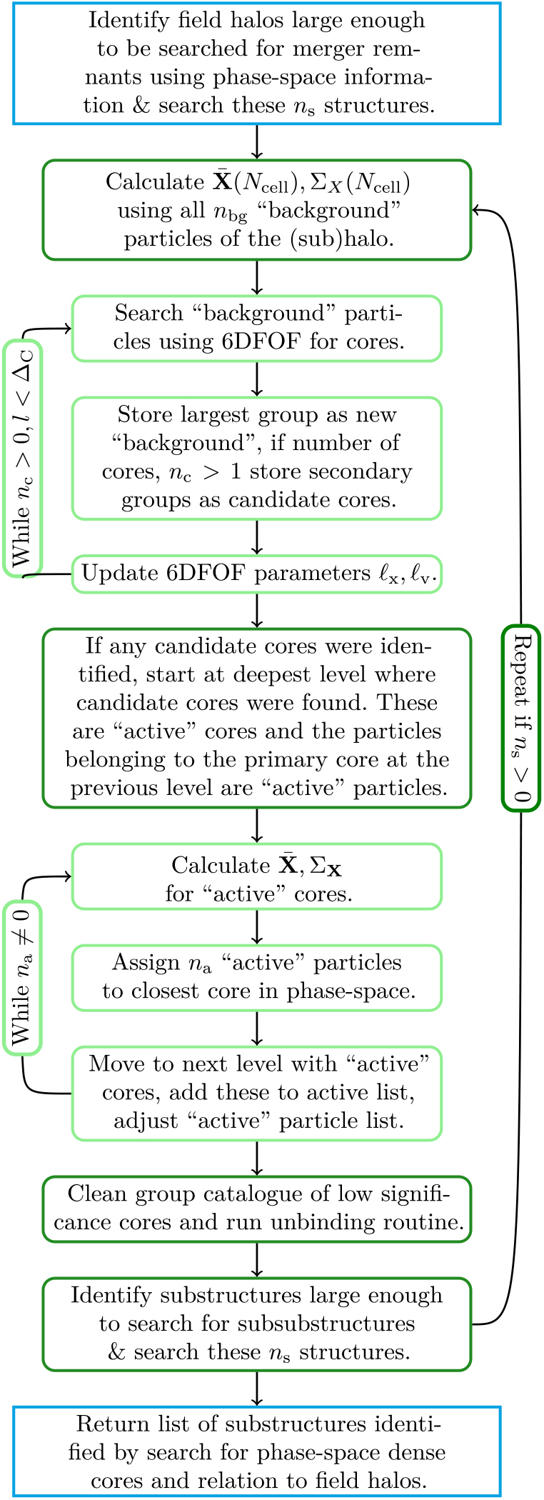
Core growth and mass reconstruction: If more than a single ‘core’ has been identified, the next step is to assign all untagged halo particles to these candidate ‘cores’ and the ‘primary core’. We start at the last iteration at which multiple groups were found, setting these ‘cores’ and ‘primary core’ as ‘active’. Phase-space dispersion tensors are calculated for these active cores:
 $$\matrix{
{\overline {\rm{X}} = {1 \over {{M_{{\rm{core}}}}}}\mathop \Sigma \limits_k^{{N_{{\rm{core}}}}} {m_k}{{\rm{X}}_k},}} $$
$$\matrix{
{\overline {\rm{X}} = {1 \over {{M_{{\rm{core}}}}}}\mathop \Sigma \limits_k^{{N_{{\rm{core}}}}} {m_k}{{\rm{X}}_k},}} $$
 $$\matrix{
{\sigma {{\rm{x}}_{{\rm{i,j}}}} = {1 \over {{M_{{\rm{core}}}}}}\mathop \Sigma \limits_k^{{N_{{\rm{core}}}}} {m_k}\left( {{X_{k,i}} - \overline {{X_i}} } \right)\left( {{X_{k,j}} - {\overline X _j}} \right).}} $$
$$\matrix{
{\sigma {{\rm{x}}_{{\rm{i,j}}}} = {1 \over {{M_{{\rm{core}}}}}}\mathop \Sigma \limits_k^{{N_{{\rm{core}}}}} {m_k}\left( {{X_{k,i}} - \overline {{X_i}} } \right)\left( {{X_{k,j}} - {\overline X _j}} \right).}} $$
We then assign untagged particles that were searched at this iteration, ‘active background particles’, to the closest active core in phase space. The distance used is:
 $$\matrix{
{D_{k,n}^2 = \left( {{{\rm{X}}_k} - {{\overline {\rm{X}} }_n}} \right)\Sigma _{{\rm{X,n}}}^{ - 1}\left( {{{\rm{X}}_k} - {{\overline {\rm{X}} }_n}} \right),}} $$
$$\matrix{
{D_{k,n}^2 = \left( {{{\rm{X}}_k} - {{\overline {\rm{X}} }_n}} \right)\Sigma _{{\rm{X,n}}}^{ - 1}\left( {{{\rm{X}}_k} - {{\overline {\rm{X}} }_n}} \right),}} $$
where here we show the distance of particle k to a core n and Σ is the matrix representation of σ Xi,j.
Once all active particles at the current level are assigned, we then move up to the previous iteration and assign particles. If cores are present at this iteration, they are added to the active core list and we proceed as outlined above. We repeat the process till all particles not associated with substructure have been assigned to a core.
This method is similar to assigning particles based on a Gaussian mixture model,Footnote i but less time-consuming as we do not calculate full likelihoods. It also has the added advantage that we do not require each distribution to be characterised by a single global dispersion tensor.
The use of phase-space tensor-based distance also has an advantage over algorithms that use a simple 6DFOF-like distance metric (see Equation (2), e.g., rockstar) as it does not impose a spherical distribution, nor ignore covariance between positions and velocities. That is not to say that for moderately aspherical distributions typical of halos, using scalar dispersions performs poorly, but that results can be improved using dispersion tensors.
We compared assigning particles using dispersion tensors to dispersion scalar using simple models composed of overlapping multivariate Gaussians. We draw particles from several n-dimensional multivariate Gaussian distributions with means roughly separated by ∼1 − 3σ from each other, and with each subpopulation containing similar numbers of members. Initial dispersion scalars and tensors are determined using 100 particles and then assign particle group membership using the relevant distance in single step. We find tensor-based distance assignment results in groups of higher purity, that is a higher fraction of correctly identified members. There is also a reduction in the group-to-group scatter in purity. The amount of improvement depends on the asphericity of the distributions, with increase of a few per cent or more. More aspherical distributions have larger increases in purity as well as the fraction of the group recovered. Iterating this process improves the results.
For example, consider particles drawn from two Gaussian distributions, one spherical, the other quite aspherical (with minor axis ratio of 0.03), separated by a phase-space tensor normalised distance of ∼ 2. Assignment using the dispersion scalar distances results in a purity of 0.76 and 0.92 for the spherical and aspherical populations, respectively. Using tensor-based distances improves the purity to 0.79 and 0.93, respectively. The recover fractions are similarly improved from 0.94 and 0.70 to 0.95 and 0.76, respectively.
Cleaning the catalogue: We clean the candidate core list of spurious objects prior to core growth by requiring that the distance of a core n to the primary core p identified at the same point to be significant,
 $$\matrix{
{D_{p,n}^2 \ge {\beta _C},}} $$
$$\matrix{
{D_{p,n}^2 \ge {\beta _C},}} $$
where the distance is based on the secondary core’s phase-space tensor using Equation (21), and β C is the significance. The substructures after core growth are then processed by the unbinding procedure (see Equation (17)).
2.4. Substructure and baryons
Assigning baryonic particles to substructure or identifying baryonic substructures depends on the mode of operation. We discuss the two principal modes here.
Substructure in DM + baryons mode: In this mode, baryons have already been assigned to an FOF envelop. For each FOF envelop, baryons are assigned to the group of the DM particle that is closest in phase space using a simple phase-space metric
 $$\matrix{
{D_{{\rm{B,DM}}}^2 = \left( {{{\rm{x}}_{\rm{B}}} - {{\overline {\rm{x}} }_{{\rm{DM}}}}} \right)/{\ell _{\rm{x}}} + \left( {{{\rm{v}}_{\rm{B}}} - {{\overline {\rm{v}} }_{{\rm{DM}}}}} \right)/{\sigma _v},}} $$
$$\matrix{
{D_{{\rm{B,DM}}}^2 = \left( {{{\rm{x}}_{\rm{B}}} - {{\overline {\rm{x}} }_{{\rm{DM}}}}} \right)/{\ell _{\rm{x}}} + \left( {{{\rm{v}}_{\rm{B}}} - {{\overline {\rm{v}} }_{{\rm{DM}}}}} \right)/{\sigma _v},}} $$
where σ v is the typical velocity dispersion of structures found.Footnote j
Substructure in galaxies + baryons mode: The process used to identify DM substructures is ill suited to separating interacting galaxies as stars are constantly being formed and there need not have a well-defined background. Instead interacting galaxies are separated using the core search as outlined in Section 2.3 (see Cañas et al. Reference Cañas, Elahi, Welker, Lagos, Power, Dubois and Pichon2018, for details). Once interacting galaxies have been separated, the same assignment scheme is used as in the DM+Baryons mode to assign other baryonic particles (gas and black hole particles) to the nearest star particle.
2.5. Halo properties
The code calculates a large number of bulk properties for each object (see Table B.2 for an almost complete list; the exact number of properties calculated depending on input). Calculating properties is complicated by the presence of substructure. Should substructures be excluded or included? The answer depends on the scientific goal. For following the evolution of objects across cosmic time using halo merger trees for input into SAMs, ideal masses are likely that of particles belonging exclusively to the object, whether halo or subhalo. This avoids abrupt changes in mass as an object transitions from a halo to a subhalo. For lensing, one is likely interested in the total mass within some region.
VELOCIraptor allows some flexibility: masses can either be calculated using particles exclusive to the object, or for halos one can include substructures. Inclusive halo masses, such as commonly used spherical overdensity halo masses,Footnote k can include particles belonging to substructures, the background and even neighbouring halos. Subhalos have exclusive masses that is calculated using only particles belonging to the subhalo. Angular momentum, like mass, can be calculated in a variety of ways for halos. Other properties, such as the maximum circular velocity, are by default calculated using particles exclusively belonging to the object.
Another complication in bulk properties has to do with the phase-space position of a halo. The overall bulk motion of particles within the FOF envelop maybe offset from the motion of the central most bound regions particularly the motions of particles near the edge of the FOF envelop (Behroozi et al. Reference Behroozi, Wechsler and Wu2013). By default, centre-of-mass positions are calculated using shrinking spheres till the last sphere encloses ∼10% of the group’s particles and velocities are calculated using this inner most 10%. These positions better characterise the orbital motion of halos, though it does not represent the overall bulk motion of mass.
VELOCIraptor also outputs all the particle IDs in each structure, so users can post-process data to calculate desired properties.
2.6. Code structure
VELOCIraptor is a C++ code that uses OpenMP+MPI APIs for parallelisation but can be compiled in serial mode, solely with OpenMP, or solely with MPI. The code requires a configuration file (example are provided with the repository), input data, and an output file name.
The code has been designed to take the following types of N-body/Hydrodynamical input: HDF5Footnote l; gadget binary format (Springel et al. Reference Springel2005); ramses binary format (Teyssier Reference Teyssier2002); and tipsy binary format (N-Body Shop 2011). For all input save TIPSY, VELOCIraptor extracts cosmological information and the spatial bounds for the particles. This information can be provided via the configuration file if not present in the input data.
The spatial extent of the particle distribution must be provided for MPI domain decomposition, even for non-periodic input. This information can be provided either via the input data itself or via the configuration file. Currently implemented MPI domain decomposition scheme is a Binary Tree like splitting.Footnote m
It produces the following types of output formats: ASCII; custom binary format; HDF5 (preferred); and ADIOSFootnote n (alpha). The output files consist of two types: a collection of bulk properties for each group; and a list of the IDs of all particles belonging to each group. It can also produce a list of particle types and even information on the file and index each particle is located at, allowing for quick extraction of particle data for further follow-up analysis. We outline a sample of the bulk properties calculated in the appendix, Table B.2.
There are a variety of configuration options available. We list the critical parameters in Table 1, providing a more complete list and the specific code parameter key words in the appendix, Table B.1. We note that for most users, these default parameters will produce standard halo catalogues and subhalo need no alteration. Most users will simply alter the minimum number of particles per halo. For identifying tidal debris, the key parameter to change is the unbinding parameter, β E, which can be set to values of ∼0.1–0.5. We highlight parameters that are likely to be changed depending on the input simulations and the desired scientific outcome.
Key VELOCIraptor parameters.
a For historical reasons, the code actually uses the substructure linking length to define the halo linking length, i.e., the code actually takes α x,H and ℓ x,S as input.
3. Results
Here we present how well halos/galaxies and substructures are identified. As input we primarily use a small cosmological N-body simulation consisting of 5123 particles (from the SURFS suite; Elahi et al. Reference Elahi, Welker, Power, Lagos, Robotham, Cañas and Poulton2018). The simulation details are presented in Table 2. For this analysis, we also make use a halo merger tree builder, treefrog (Elahi et al. Reference Elahi, Poulton, Tobar, Lagos, Power and Robotham2019). This related software is a so-called ‘Tree Builder’, software that takes as input halo catalogues across cosmic time and reconstructs the history of a halo, producing halo merger trees. Details of how TREEFROG reconstructs halo merger trees can be found in Elahi et al. (Reference Elahi, Poulton, Tobar, Lagos, Power and Robotham2019). Here we summarise the salient points: the code uses particle IDS and the group to which they belong to compare one snapshot to the next, identifying descendants by maximising a merit function that effectively links halos at a time t 1 to halos found a later time that share the largest number of most bound particles. We also compare results to three different (sub)halo finders: ahf (Knollmann & Knebe Reference Knollmann and Knebe2009), a configuration-space-based finder; rockstar (Behroozi et al. Reference Behroozi, Wechsler and Wu2013), a phase-space finder; and HBT+ (Han et al. Reference Han, Cole, Frenk, Benitez-Llambay and Helly2018), a 3DFOF tracker that uses 3DFOF halos found across all snapshots and tracks particles assigned to 3DFOF halos as they enter larger 3DFOF halos to build a halo merger tree as well as a subhalo hierarchy.
Simulation parameters.
We start by looking at the identification and decomposition of individual objects and then look at the statistical properties of the ensemble population extracted from our simulations. We use a particle limit of N min=20 and focus on self-bound objects, that is we use β E = 0.95 (see Equation (17)).
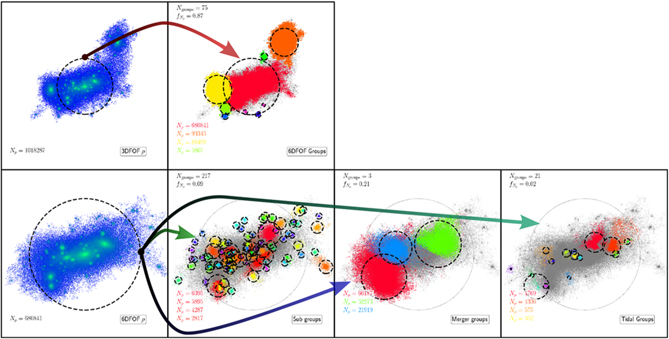
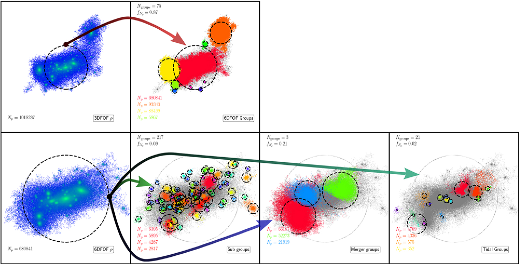
Halo decomposition: we show the process of running the routines that decompose an initial FOF candidate into 6DFOF Halos (top row), followed by the search for substructure (using Section 2.2) and major mergers (using Section 2.3) in the largest 6DFOF halo (bottom row, red 6DFOF halo seen in top right panel). The bottom panel shows the application of substructure finding (green arrow), core identification and grow for mergers (purple arrow), and the substructures identified when the self-boundness criteria are relaxed to find tidal debris (teal arrow). For each object we show R ρ by a dashed black circle. In the left column, particles are colour-coded according to the 3D density going from blue to green in increasing density. In the other panels (group sub-panels), particles are colour-coded by the group to which they belong. In these group sub-panels: we limit the number of groups displayed to those composed of more than 100 particles for clarity; list the total number of groups; the fraction of mass in these groups; the number of particles for the four largest such groups; and show the parent halo’s particles and R ρ with grey points and a grey circle, respectively.
3.1. Individual halo
Figure 4 shows a 3DFOF halo extracted from the L40N512 simulation and how each step in VELOCIraptor decomposes the candidate/parent object. In this example, we use a large halo composed of ≈106 particles identified at z = 0 with a 3DFOF mass of 4.2 × 10¹⁴ h−1M⊙ and a mass M ρc = 2.7 × 10¹⁴h−1M⊙, where M Δρc = 4π ρ cR Δρc/3, ρ c is the critical density, and R Δρc is the radius enclosing an average density of ρ c, where Δ = 200, commonly referred to as the virial mass. This 3DFOF object was identified using the standard linking length of ℓ x = 0.2L box/N p, where L box/N p is the inter-particle spacing.
The initial 3DFOF halo clearly consists of several large density peaks, some of which are well outside the virial radius centred on the largest density peak. All the density peaks would be considered subhalos of the FOF envelop, save for the peak that has the largest mass associated with it, which is considered the parent halo. This subhalo/halo definition is less than ideal as some of the larger peaks are well outside the virial radius. Moreover, some of these peaks are spuriously linked to the primary via a thin particle bridge by the FOF algorithm. This example illustrates the need for more sophisticated algorithms.
Applying the 6DFOF algorithm separates the initial 3DFOF candidate into 75 (bound) groups, 3 of which are composed of ≳ 10% of the original 3DFOF object’s particles. Approximately 87% of the original 3DFOF object’s particles are still within a group, with the largest object containing 68% and having approximately the same virial mass as the original 3DFOF. The 6DFOF algorithm produces a better mapping of an FOF object to the physical definition of a halo, that of a virialised overdensity.
The largest 6DFOF halo itself appears to contain at least four large density peaks and numerous smaller ones. If we search for substructure by identifying locally dynamically distinct particles and linking them with a phase-space algorithm (method outlined in Section 2.2), we find 217 groups containing ≈9% of the mass of the halo, the few largest of which each contain ≈1% of the total halo’s mass.
The largest density peaks within the 6DFOF are separated into three groups plus the main halo by the core search (see Section 2.3). These objects, remnants of minor/major mergers, contain 21% of the initial host halo’s mass, with the smallest containing 3% and the largest 9%. The second largest merger remnant happens to be close to the main halo, making particle assignment during the core growth phase non-trivial, particularly for the outer regions that overlap in phase space with the host. The sharp boundary between the object and the main halo is a result of a compromise between computational efficiency and rigour as we use few steps to grow cores and a global phase-space tensor to assign particles based on their distance to the cores’ centre-of-masses. Finer steps would reduce the sharpness of this transition, but as it effects small amounts of mass, extra steps are unnecessary.
For comparison, other methods find similar amounts of mass, though there are some differences. HBT+, which tracks halos, assigns the least amount of mass to the most distant object. ahf underestimates the mass of the most central object relative to all other finders, expected given its configuration-space approach. rockstar, which has a similar approach to that outlined in Section 2.3, returns similar, if typically larger masses. Both VELOCIraptor and ROCKSTAR also give similar results to a full Gaussian mixture model using centre-of-mass of the cores as initial guess.Footnote o
Phase-space distribution of substructures in the halo: We plot the radial position and velocity (scaled by the host halo properties) of all substructures found in the example 6DFOF halo with points colour-coded by mass (and scaled by mass as well). We plot minor/major mergers as square points and all other substructures as circles. We also plot the escape velocity envelop (solid black lines), circular velocity envelop (dotted grey lines), and the scale radius of the NFW concentration (vertical dashed line). We plot the large 6DFOF halos that were part of the initial 3DFOF envelop as diamonds with blue outlines, with points colour coded and scaled by mass. Finally we also plot any objects not considered part of the initial 3DFOF and within 3R 200ρ as grey diamonds to show the halo population (and subhalos in other halos) in the surrounding environment.
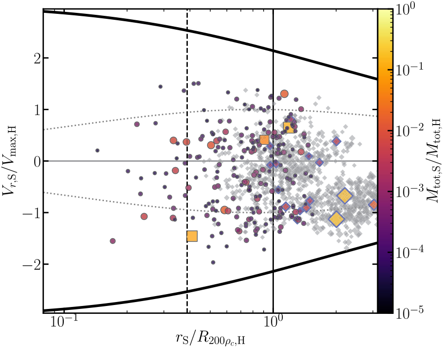
The phase-space distribution of these objects within of the parent halo is presented in Figure 5. Here we focus on the objects found within the 6DFOF envelop and use the total mass exclusively assigned to an object, M tot.Footnote p The relative velocities and radial distances of the subhalos are scaled by maximum circular velocity of the host and its virial radius. We also show the largest halos that were separated by the 6DFOF from the initial 3DFOF envelop.
The radial motions (as well as the total relative velocity) of all subhalos belonging to the 6DFOF envelop are well within the escape velocity envelop. For this particular halo, the parent 3DFOF halo would have linked together several objects that are on first infall and lie outside the virial radius, again pointing to a better mapping between a 6DFOF object and a virialised overdensity, a.k.a, a halo. For example, the typical apocentre for particles orbiting a halo is ∼1.6–1.9R 200crit (though the exact value depends on the mass accretion rate of a halo and the rarity of the halo, for 75% of a halo’s particles apocentres are ≈1.0–1.2R 200ρm, where R 200ρm ≈ 1.6R 200ρc, see Diemer et al. Reference Diemer, Mansfield, Kravtsov and More2017). The two largest objects separated by the 6DFOF algorithm are well outside the virial radius at similar distances of ≈2R 200ρc,H . However, they have large infalling radial velocities of ≈− 0.9V max,H, significantly different from most particles that have completed at least one orbit of their host halo. Following their history using a halo merger tree (built with TreeFrog; Elahi et al. Reference Elahi, Poulton, Tobar, Lagos, Power and Robotham2019), we see that they are on first infall, as are most of the halos within the surrounding environmentFootnote q (as seen by the grey diamonds with negative velocities in Figure 5).
Inner subhalo: We show a subhalo identified within the scale radius of a host halo. We plot its configuration space (top) and velocity space (bottom) distribution. Particles belonging to the subhalo are plotted as large circles, the background halo as small points, with points colour-coded by log ρ, increasing in density going from blue to green. In the top panel, we mark the centre-of-mass by a ‘+’, its R 200ρ by a dashed circle. We also mark the center of the parent halo by a ‘x’ and also show the scale radius by a dashed red circle (seen in the left corners). In the bottom panel, we plot the centreof-mass velocity with a ‘+’ and V max by a dashed circle. The parent halo’s centre-of-mass velocity is off the plot in the direction of the red arrow. We also plot the parent halo’s Vmax,H by a red dashed circle (seen in the top corner) and also plot an ellipse centred on the mean velocity of the background particles in the nearby volume with its size scaled by the standard deviation (seen in lower-right corner). For both panels we plot a ruler to give a sense of scale.
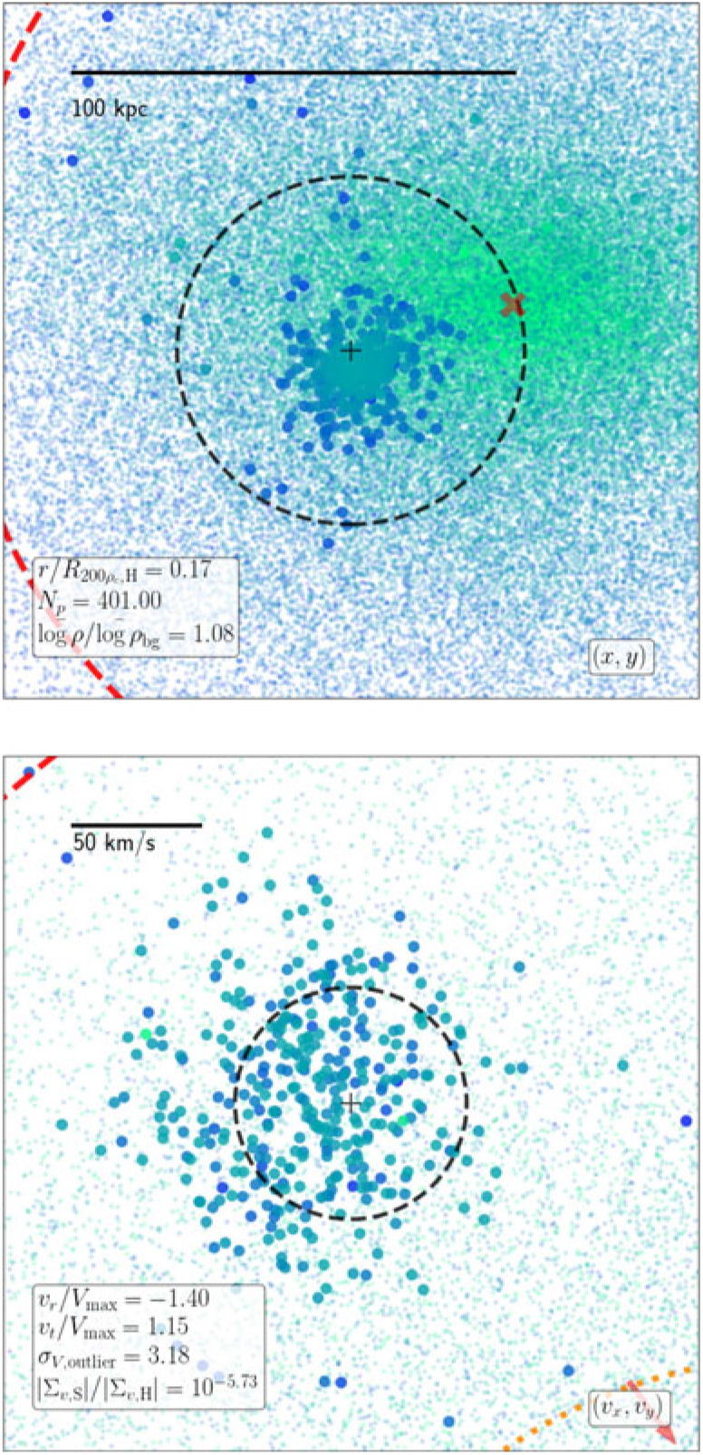
The inner most subhalos highlight the benefit of a phase-space finder. As an example, we focus on the large infalling subhalo located at ≈0.2R 200ρc,H and its surroundings, presented in Figure 6. In configuration space, the subhalo has a similar density to the background halo. It is only in velocity space that the subhalo becomes readily apparent. The object is a local velocity outlier as it lies outside the local velocity dispersion. The extent to which this object centre-of-mass motion V S relative to the local surroundings is an outlier is given by
 $$\matrix{
{{\sigma _{V,{\rm{outlier}}}} \equiv {{[\left( {{{\rm{v}}_{\rm{S}}} - {{\overline {\rm{v}} }_{{\rm{bg}}}}} \right)\Sigma _{v,{\rm{bg}}}^{ - 1}\left( {{{\rm{V}}_{\rm{S}}} - {{\overline {\rm{v}} }_{{\rm{bg}}}}} \right)]}^{1/2}},}} $$
$$\matrix{
{{\sigma _{V,{\rm{outlier}}}} \equiv {{[\left( {{{\rm{v}}_{\rm{S}}} - {{\overline {\rm{v}} }_{{\rm{bg}}}}} \right)\Sigma _{v,{\rm{bg}}}^{ - 1}\left( {{{\rm{V}}_{\rm{S}}} - {{\overline {\rm{v}} }_{{\rm{bg}}}}} \right)]}^{1/2}},}} $$
where ${\overline {\rm{v}} _{{\rm{bg}}}} $ and ${\Sigma _{v,{\rm{bg}}}} $
 are the local mean velocity and velocity dispersion tensor. We find that its centre-of-mass velocity is a ≳3σ outlier of the local velocity distribution. Moreover, the particles belong to the object are far more clustered about its velocity than the expectation, with the ratios of the dispersion tensors giving 2 × 10⁻⁶.
To compare the particles belonging to the substructure to the background, we randomly sample the background particles 1 000 times using the same number of particles belonging to this subhaloinaregion centredonthe subhalowithinaradius of 1.5R 200ρc. We find velocity differences of σ V,outlier = 3.27 ± 0.18, dispersion ratios of |σ S|/|Σ bg|= (1.6 ± 0.2) × 10−6, and density = 1.02 ± 0.02. The object’s mean density is similar to the background yet the subhalo’s centre-of-mass velocity is a significant outlier and its velocity dispersion is much colder.
The low density contrast does not necessarily mean that this object cannot be recovered by configuration-space finders. For instance, AHF does recover this object; however, the object proceeds to shrink as it enters deep within the host. Moreover, the initial collection of particles within the density peak will contain both particles belonging to the subhalo and those of the background, which must be carefully pruned by an unbinding process. By using velocity information, the particles belonging to the object can be robustly separated from the background, particularly the more underdense outer regions, minimising the amount of cleaning that must be done.
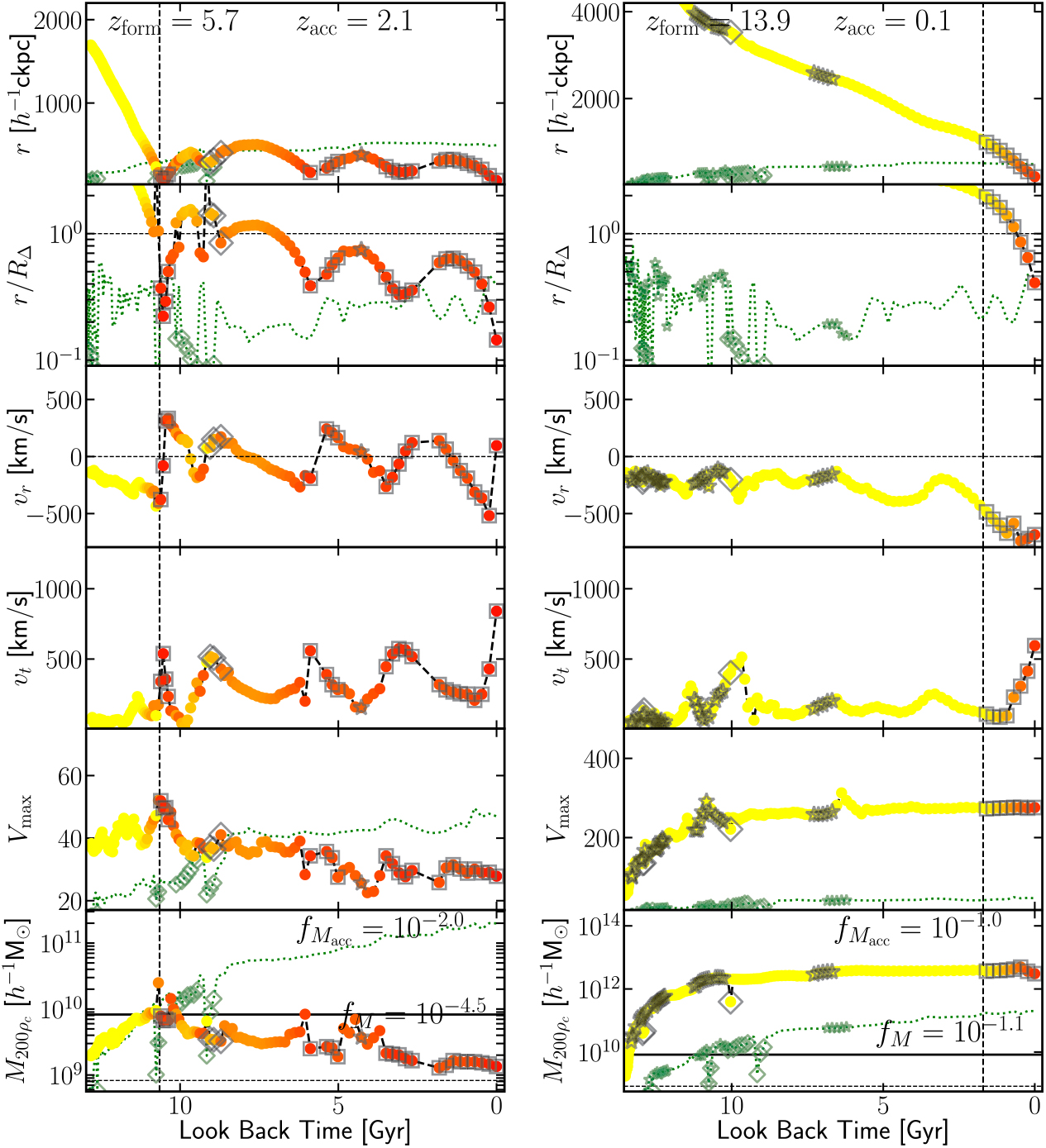
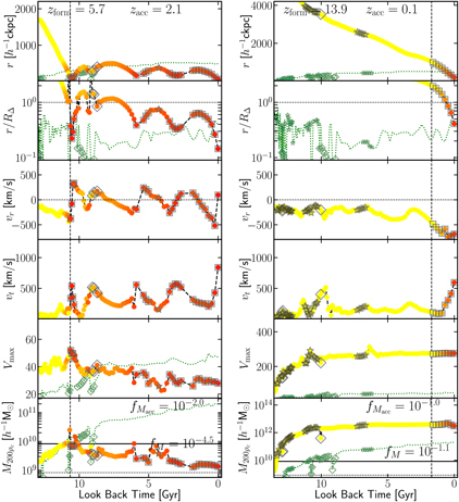
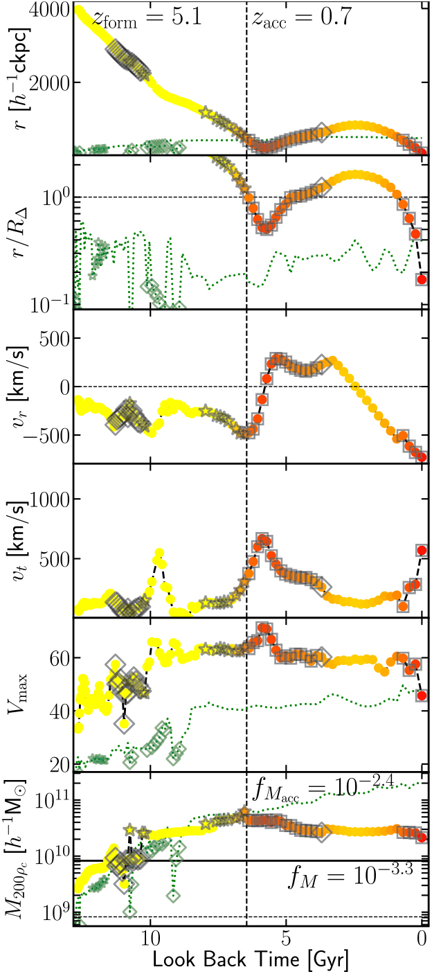
The low density contrast might also suggest that this object is perhaps artificial, despite being identified by VELOCIraptor, AHF, and rockstar. To verify its physical origin, we must examine its history. We find that it is present in HBT+ catalogue and thus must have originated from a 3DFOF halo. We show the mass accretion history as reconstructed by TreeFrog (Elahi et al. Reference Elahi, Poulton, Tobar, Lagos, Power and Robotham2019) from the VELOCIraptor catalogue along with its radial motion, radial and tangential velocities, and maximum circular velocity in Figure 7, highlighting how well VELOICraptor works (see Figure C.1 in Appendix A for more examples).
At z = 0, this subhalo is found on a primarily radial orbit deep within the host. This object’s first progenitor formed at a redshift of z form = 5.1 with 32 particles and gradually moves closer to the main branch of the host halo. On its way, it experiences a significant merger event at high redshift, i.e., it contains a subhalo that has a mass ratio of ≥1:10 as indicated by the open diamond and open stars surrounding its track. This merger event also corresponds to when it experiences significant fluctuations in mass & V max. The fluctuations are quite severe, changing masses by factors of ∼2, as the object is not well resolved at this time, composed of ∼200 particles. The fluctuations in mass are also partially due to the fact that masses for subhalos are exclusive, whereas for field halos, the mass includes substructure. At these high redshifts, the main branch also experiences several major mergers, giving rise to mass fluctuations and changes in the relative motion of the subhalo to the host.
Prior to its accretion, the object contains a single large substructure containing ∼25% of its total mass. The sudden drop in mass upon accretion is due to subhalo masses being exclusive in VELOCIraptor. Critically, the mass evolution after accretion is physically reasonable. Little mass is lost till pericentric passage, at which the system is shocked, increasing its V max (and R (V max)). After this impulsive heating, the halo begins to lose mass, the rate of mass loss decreasing as it reaches apocentre, which lies outside the halo at 2R 200ρc. The object then plunges radially through the halo. The slight kinks in the radial and tangential velocities during this radial infall here are due to the host halo merging with a subhalo with a mass ratio of 1:6. The central regions of the main halo consist of two overlapping phase-space distributions with slightly different velocities that are rapidly phase-mixing. VELOCIraptor is no longer able to disentangle these objects, causing a small amount of jitter in the centre-of-mass velocity of the host.
Reconstructed subhalo orbital and evolution: We plot the orbit and evolution of the subhalo presented in Figure 6 as a function of look back time. Top two sub-panels show radial distances of the object to the main branch of its z = 0 host, in comoving units and relative to host R 200ρ , respectively. Next two sub-panels show relative radial and tangential velocities. Bottom two sub-panels show the object’s V max & M 200ρ evolution. Points are colour coded by radial distance from host. We also highlight points: squares indicate when the object is a subhalo of the host main branch, diamonds signify that the object is a subhalo of another halo, and stars indicate the object itself has ≥ 20% of its own mass in substructure. For all sub-panels we show the accretion time by a dashed vertical line. We also show several properties of host main branch by a dotted green line: R 200ρ in the top sub-panel; scale radius in the second sub-panel; V max/10 in the fifth sub-panel; and M 200ρ/100 in the sixth sub-panel. We also highlight when the host main branch is a subhalo or contains significant amounts of substructure by a diamond and star, respectively.
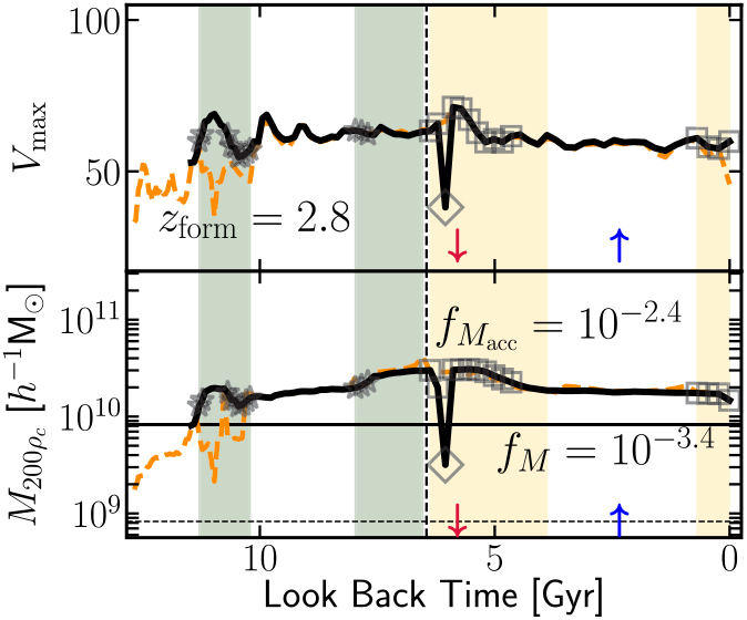
For comparison, we examine the counterpart identified by AHF, a configuration-based finder, which identifies a subhalo despite the low density contrast. The object in the AHF catalogue is similar if lower mass at the last snapshot. As the orbital reconstructed orbital motion is similar, we focus on mass and maximum circular velocity evolution in Figure 8, highlighting where the object is a subhalo and has itself significant substructure. We also show the evolution of the VELOCIraptor object and highlight with shaded regions where the object contains significant substructure or is a subhalo. This figure shows that both codes recover similar mass evolution save for two key differences. The AHF subhalo experiences a rapid mass fluctuation in mass, dropping by an order of magnitude as the object approaches pericentre where density contrasts are low. The object also forms much later when composed of ∼200 particles, during a period where the object is undergoing a major merger. In the AHF catalogue, the object is lost for a few snapshots, truncating the halo merger tree. This figure indicates that in general both configuration-space and phase-space finders perform well, and it is only during pericentric passages and major mergers that phase-space-based finders outperform configuration-space-based ones.
Reconstructed AHF subhalo evolution: We plot the V max & M 200ρ evolution of the AHF counterpart to the subhalo presented in Figure 6 as a function of look back time. We plot the AHF object with a solid black line, the VELOCIraptor object with a dashed orange line. Similar to Figure 7, we highlight when the object is a subhalo of the host main branch, a subhalo of another halo, and when the object itself has ≥20% of its own mass in substructure. We also highlight periods when the VELOCIraptor object has significant substructure or is a subhalo by a shaded green and shaded yellow region, respectively. We indicate when pericentric and apocentric passages occurs by ↓ & ↑, respectively. For all sub-panels we show the accretion time by a dashed vertical line.
The other instance where a phase-space finder like VELOCIraptor outperforms configuration-space-based ones is in recovering tidal debris. Tidal debris is not spatially overdense and requires measurement of the local velocity density. By using the local velocity density, VELOCIraptor naturally identifies a continuum of substructures from bound subhalos to unbound dynamically cold streams. This initial catalogue is cleaned by invoking an unbinding process. If we relax the unbinding criterion and also use the two stage iterative procedure described in Section 2.2 to retain tidal features and debris, we have the structures shown in the bottom-right sub-panel of Figure 4, where we have limited the groups to those that have at most 50% of their particle’s bound. These objects consist of tidal shells originating from the larger merging subhalos and subhalos with large, extended tidal tails. For a thorough discussion of tidal debris, see Elahi et al. (Reference Elahi2013). Here we will focus on the recovered subhalo distribution.
3.2. Population
3.2.1. Halos
We examine the impact of and the results from each stage of the algorithm using default parameters. We start by looking at halos identified with 3DFOF versus a 6DFOF. Using a 6DFOF does not significantly alter the input 3DFOF population as, on average, 3DFOF halos contain a 6DFOF object with $0.82_{ - 0.10}^{ + 0.07} $ of the mass of the original FOF object, independent of the number of particles in the 3DFOF as seen in Figure 9. Consequently, the 6DFOF mass function should show a small suppression in mass relative to the 3DFOF mass function. The number of 6DFOF objects per 3DFOF group increases with increasing number of particles in the 3DFOF group as seen in Figure 9.
6DFOF to 3DFOF stats: we plot the fraction of particles in 6DFOF groups per 3DFOF group (blue solid), the fraction in the largest 6DFOF group (dashed cyan), and the number of 6DFOF groups per 3DFOF (right y-axis, red dotted line) as a function of the number of particles in the 3DFOF group. For each curve we plot the median, 16% and 84% quantiles.
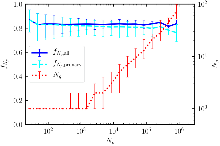
Due to resolution limits, not all 3DFOF objects contain a viable 6DFOF halo, particularly close to the imposed particle threshold of 20, where only 50% of 3DFOF objects have a 6DFOF halo above this threshold. The absence of a 6DFOF halo in a 3DFOF object drops to ≲1% for 3DFOF objects composed of ∼100 particles. These objects are typically highly unrelaxed, unbound 3DFOF objects, i.e., spurious 3DFOF objects.
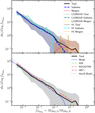
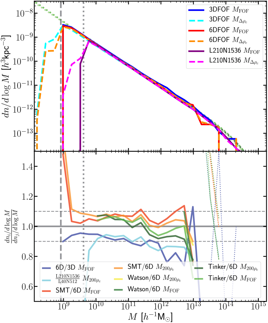
The resulting halo mass from the different FOF algorithms and N-body simulation are shown in Figure 10. For FOF masses, the 6DFOF mass function is effectively the 3DFOF mass function shifted to the left by ≈0.1 dex (as on average 6DFOF halos contain 80% of the original 3DFOF halo’s particles). The virial mass remains unchanged when comparing the 3DFOF halo to the largest 6DFOF object within the 3DFOF halo, with small mass differences due to small differences in the centre-of-mass. However, as there are on average 1.3 6DFOF groups per 3DFOF halo, the 6DFOF virial mass function has more halos per mass bin. The peak the virial mass distribution at low masses arises from loosely bound, poorly resolved halos with low overdensities.
The residuals show that the 6DFOF mass function has fewer objects than the 3DFOF one at a given M fof, asexpected. We also compare the 6DFOF algorithm to three models, Sheth et al. (Reference Sheth, Mo and Tormen2001), Tinker et al. (Reference Tinker, Robertson, Kravtsov, Klypin, Warren, Yepes and Gottlöber2010), and Watson et al. (Reference Watson, Iliev, D’Aloisio, Knebe, Shapiro and Yepes2013). These models span a range of algorithms used to find halos and the type of mass recorded. Sheth et al. (Reference Sheth, Mo and Tormen2001) and Watson et al. (Reference Watson, Iliev, D’Aloisio, Knebe, Shapiro and Yepes2013)use 3DFOF algorithms, whereas Tinker et al. (Reference Tinker, Robertson, Kravtsov, Klypin, Warren, Yepes and Gottlöber2010) used to a spherical overdensity finder. Watson et al. (Reference Watson, Iliev, D’Aloisio, Knebe, Shapiro and Yepes2013) uses M FOF,whereasthe other two use M 200ρc. The 6DFOF relative to the models has fewer objects per mass bin. The systematic shift is of the same size as going from 3DFOF to 6DFOF. This is partially due to the 6DFOF naturally decomposing 3DFOF objects into dynamically distinct halos, although there are other systematic effects between the simulation and the theoretical curves arising from the finite volume of the box.Footnote r We also compare our reference simulation to our larger volume, lower mass resolution simulation, L210N1536. The simulations agree to within ≲5% for well-resolved halo masses of ≳5 × 10⁹ h−1M⊙, though the larger volume simulation contains slightly fewer halos with M 200ρc ≲1010.5 h−1M⊙.
Halo mass functions: we plot halo mass function measured using the 3DFOF and 6DFOF algorithm. The top panel shows the mass function along with several models, plotted as green coloured dashed lines. In the bottom panel we plot the radio of an interesting subset of results and models, with models calculated using HMFCALC (Murray, Power, & Robotham Reference Murray, Power and Robotham2013). Lines are thin at high masses when the number of halos in a given mass bin is below 10, i.e., the statistical variation exceeds 25%.
The velocity function, not presented here for brevity, is effectively unchanged save for the fact that the 6DFOF is able to decompose 3DFOF objects into multiple halos, increasing the amplitude of the 6DFOF relative to the 3DFOF for well-resolved halos with V max ≳30 km/s.
3.2.2. Subhalos
We next examine the results of subhalo/core search for our example halo and the population as a whole. To determine the average subhalo mass function we stack all halos composed of ≥50 000 particles, i.e., all halos that at least probe the subhalo mass function down to masses fractions of f M ≥ 5 × 10⁻⁴, with halo masses of f M200ρc ≳ 2 × 10¹² h−1M⊙. There are 128 such halos in our reference simulation. We focus on overdensity mass ratios f M200ρc ≡ M 200ρcS/M 200ρcH presented in Figure 11 (although using the total mass dynamically associated with a substructure relative to the dynamical mass exclusively associated with the parent subhalo, f Mtot ≡ M tot,S/M tot,H does not significantly change the resulting mass function). For consistency across catalogues, we identify all objects with the virial radius of the host as subhalos. Here we classify substructures based on the specific method used to identify them to highlight any differences in the distribution arising from the methods: objects identified by the phase-space FOF algorithm on dynamically distinct particles (Section 2.2) are here referred to as subhalos; objects identified by searching for phase-space dense cores (Section 2.3) in the parent halo are classified as mergers (containing both major and minor merger events with mass ratios of ≳0.05). This categorisation does not imply a hard physical difference between objects, and it is simply to highlight any algorithmic differences. We also classify objects identified within substructures, the so-called subsubstructures as subhalos.
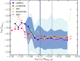
Subhalo mass function: We plot the median subhalo mass function plus the 1σ scatter for all halos composed of >=50 000 particles. We split the VELOCIraptor mass function into two categories, subhalos and mergers. We also show the median distribution from a larger-volume, lower mass-resolution simulation L210N1536 and that from our fiducial example halo, H1. In the lower panel, for comparison, we show the power-law fit and the median distribution from AHF, ROCKSTAR,and HBT+ using the L40N512 box, along with a best fit model and the model from Han et al. (Reference Han, Cole, Frenk, Benitez-Llambay and Helly2018).

On average, halos contain a total of $\mathop {208}\nolimits_{ - 130}^{ + 22} $ subhalos with over-density masses of f M200ρc ≳7 × 10⁻⁵ (with the numbers increasing if looking at total dynamical masses with the same limit of f M tot ≳ 7 × 10⁻⁵ to $\mathop {272}\nolimits_{ - 177}^{ + 61} $
 . Halos contain at least 1 subhalo with a mass of f M 200ρc ∼ 10−2. Significant merger events are not uncommon, with an average number per halo of 1.7 ± 1.6. The example halo contains subhalos with 10−5 ≲ f M200ρc ≲10-2 and contains three large merger remnants with mass fractions of f M200ρc ≳ 4 × 10⁻² The fiducial halo has more substructure than the average (it lies close to the +1σ envelop), which is not unexpected given the number of merger remnants it contains and the fact that this 6DFOF halo lies at the nexus of three large merging halos (see Figure 4).
The median and halo-to-halo scatter seen in our small volume simulation are in agreement with that seen in our large volume, lower-mass resolution simulation, L210N1536, when applying the same particle number threshold (for clarity we only show the median for this simulation). The median distribution from L210N1536 is based on 3 000 halos with a higher median masses of M 200ρc ≈ 3 × 10¹³ h−1M⊙. The agreement between different host halo masses indicates a mostly scale-free subhalo mass function.
For comparison, we also show the results from AHF,a configuration-space-based halo finder, ROCKSTAR, a phase-space halo finder, and HBT+, a 3DFOF tracker. These mass functions agree within the scatter modulo differences in the definition of subhalo masses, which vary from halo finder to halo finder (see Knebe et al. Reference Knebe2013b, for a discussion of mass definitions). VELOCIraptor can report a variety of different masses: bound mass, total dynamical mass, overdensity masses, etc. The first two masses are calculated using an exclusive particle list. For halos, it calculates inclusive spherical overdensity masses. For subhalos, all these masses are calculated based on a list of particles belonging exclusively to the object, neglecting the background host and internal substructures. ROCKSTAR also calculates masses for subhalos in a similar fashion using exclusive particle lists. ahf calculates inclusive spherical overdensity masses defined by a saddle point and processed through an unbinding procedure, so most resembles the spherical overdensity masses of VELOCIraptor and rockstar. HBT+ returns bound masses based on the initial FOF envelop and does not allow subhalos to accrete mass from their surrounding host halo, though they can accrete material from subsubhalos, those objects that were subhalos when the object itself was an FOF halo. This mass best corresponds to the total bound mass calculated by VELOCIraptor.
Although the mass functions agree, there are systematic differences in the number of subhalos per halo found by each finder. Given the high cadence of the input 3DFOF catalogue,Footnote s HBT+ is a useful reference catalogue. VELOCIraptor finds similar numbers of objects composed of ≥20 particles within R 200ρc of large halos as HBT+, identifying 98% ± 7% of all 3DFOF halos tracked, some of the variation due to differences in the centreof-mass. AHF finds a slightly smaller percentage of 84% ± 10%, the lower number arising from small, low-density subhalos. The outlier is rockstar, which identifies a factor of $\mathop {1.85}\nolimits_{ - 0.2}^{ + 0.15} $ more objects, though a significant fraction appear to be diffuse, possibly spurious, phase-space structures with low M 200ρc, with some never reaching overdensities of 200ρ c. Removing these low density objects from the halo catalogue places it more in line with the other codes, though it still identifies a factor of $\mathop {1.05}\nolimits_{ - 0.05}^{ + 0.1} $
 more objects than HBT+.
The average subhalo distribution is well characterised by a power-law with an exponential dampening at the high mass. We fit the average mass function using emcee(Foreman-Mackey et al. Reference Foreman-Mackey, Hogg, Lang and Goodman2013) with
 $$\matrix{
{{\rm{d}}n/{\rm{d}}{{\rm{f}}_M} = Af_M^{ - \alpha }{\rm{exp[ - }}{{\left( {{f_M}/{f_o}} \right)}^\beta }{\rm{],}}}} $$
$$\matrix{
{{\rm{d}}n/{\rm{d}}{{\rm{f}}_M} = Af_M^{ - \alpha }{\rm{exp[ - }}{{\left( {{f_M}/{f_o}} \right)}^\beta }{\rm{],}}}} $$
focusing on subhalos explicitly (that is, those objects identified by the method outlined in Section 2.2 with typical mass ratios of f M ≲10−2), and ignore minor/major merger remnants (objects identified by the method outlined in Section 2.3 with typical mass ratios of f M ≳ 10−2). We find ${\rm{log }}A = - \mathop {1.7}\nolimits_{ - 1.0}^{ + 0.7} ,\alpha = \mathop {1.85}\nolimits_{ - 1.18}^{ + 0.16} ,{\rm{ }}\log {f_0} = - 1.33 \pm 0.9,\beta = 3.2 \pm 1.9 $ for M 200ρc, though the fit does not vary drastically if we use total masses. The amplitude and power-law are consistent with the previous studies (e.g. Madau, Diemand, & Kuhlen Reference Madau, Diemand and Kuhlen2008; Springel et al. Reference Springel2008; Stadel et al. Reference Stadel, Potter, Moore, Diemand, Madau, Zemp, Kuhlen and Quilis2009; Gao et al. Reference Gao, Navarro, Frenk, Jenkins, Springel and White2012; Onions et al. Reference Onions2012; Rodríguez-Puebla et al. Reference Rodríguez-Puebla, Behroozi, Primack, Klypin, Lee and Hellinger2016; van den Bosch & Jiang Reference van den Bosch and Jiang2016; Han et al. Reference Han, Cole, Frenk, Benitez-Llambay and Helly2018). The scale of the exponential dampening occurs at f M ≈ 0.05, in agreement with recent studies (e.g. van den Bosch & Jiang Reference van den Bosch and Jiang2016; Han et al. Reference Han, Cole, Frenk, Benitez-Llambay and Helly2018).
Large mass ratio objects, that is minor and major mergers, appear to be characterised by a skewed-Gaussian-like distribution. The fact that mergers follow a different distribution than subhalos is not surprising as once objects are large enough, they become less prone to tidal stripping and more affected by dynamical friction. Given number of merger remnants in this data set, we refrain from fitting the distribution, though the average of log f M200ρc, mergers = −1.2 ± 0.8 is in agreement with Elahi et al. (Reference Elahi, Welker, Power, Lagos, Robotham, Cañas and Poulton2018), who used a larger data set to fit results. We find that the total subhalo mass function also agrees with the double power-law fit in Han et al. (Reference Han, Cole, Frenk, Benitez-Llambay and Helly2018), although the second power-law describing the high mass end is poorly constrained with values of 1.1 − 1.5 [for completeness we show the double power-law from Han et al. (Reference Han, Cole, Frenk, Benitez-Llambay and Helly2018) in the figure].
Subhalo radial distribution: We plot the number density of subhalos. Similar to Figure 11, we limit the analysis to halos composed of >=105 particles (so as to probe well inside the virial radius). The average scale radius and the 1σ scatter are shown by solid and dashed vertical lines, respectively.
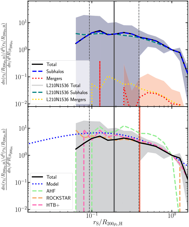
The fact that the total subhalo mass function (subhalos+-mergers) is not characterised by a single power-law is also seen in Han et al. (Reference Han, Cole, Frenk, Benitez-Llambay and Helly2018) (see also HBT+in Figure 11). They argued for characterising the subhalo mass function by a double Schetcher function with a steep power-law for low mass fractions and a flatter that dominates at high mass fractions. Given the small number of large subhalos, which also span a very small range in f M, it is difficult to differentiate between either model with the number of host halos in this sample and the halo-to-halo scatter.
The radial distribution of subhalos in the form of the differential number density dn/dV normalised by the number of objects at the virial radius is shown in Figure 12. We limit our sample to halos composed of ≥105, as these halos contain significant amounts of substructure and have density profile converged to radii of ≈10−2R 200ρc (Power et al. Reference Power, Navarro, Jenkins, Frenk, White, Springel, Stadel and Quinn2003).
We fit a generalised NFW-like profile to the distribution:
 $$\matrix{
{dn/dv\alpha {{\left( {r/{r_s}} \right)}^{ - \alpha }}{{\left( {1 + r/{r_s}} \right)}^{ - \beta }},}} $$
$$\matrix{
{dn/dv\alpha {{\left( {r/{r_s}} \right)}^{ - \alpha }}{{\left( {1 + r/{r_s}} \right)}^{ - \beta }},}} $$
where r s is the scale radius, and α and β represent the inner and outer slopes. This fit is motivated by the fact that halo DM density profiles follow this profile with α = 1 and β = 2. Subhalos should be radially distributed in a way similar to the smoothly accreted DM. We find an optimal fit of r s = 0.4 ± 0.1R 200ρc, α = 0.10 ± 0.23, and $\beta = \mathop {3.85}\nolimits_{ - 0.23}^{ + 0.11} $ . This profile that is flatter than a halo density profile in the inner regions, in agreement with previous studies (see for instance Han et al. Reference Han, Cole, Frenk and Jing2016, where they find an inner slope of ∼0.3 for a very well resolved 1012 h−1M⊙ halo, a fit that well describes halos over a wide range in masses.), although our halos are not well resolved enough precisely constrain the exact slope of the inner profile. Only very high resolution zoom simulations, such as Aquarius Springel et al. (Reference Springel2008), contain enough subhalos to properly constrain the inner slope and even then, since subhalos spend most of their time at apocentre and not pericentre, few subhalos are present in the very central regions for long.
Subhalo radial-mass distribution: we plot median subhalo mass at a given radius as a solid blue line, along with the 16, 84 and 2.5, 97.5 quantiles as filled blue and cyan regions. The average scale radius and the 1σ scatter of host halos is shown by solid and dashed vertical lines respectively. We also show the median distribution for our L210N1536 run, AHF, ROCKSTAR,and HBT+.
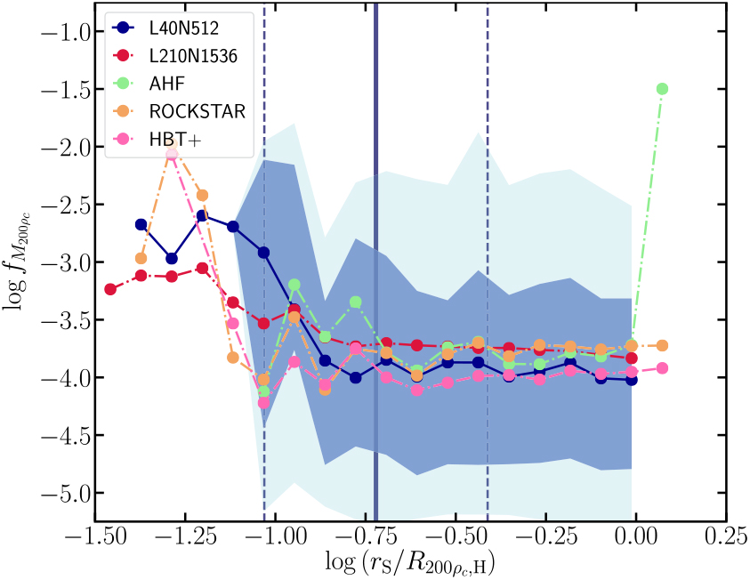
The second power-law index implies that the logarithmic slope dln n/dln r = −α − β (r/r s) / (1 + r/r s) is steeper than a NFW profile and even our fit does not capture the steep slope of the subhalo distribution. However, we stress that at the virial radius, both the subhalo radial distribution and the halo density profiles have similar logarithmic slopes of approximately −2.8. Only at even larger radii do subhalos drop off faster than an NFW profile.Footnote t
Comparing results, we find that the median distribution from the larger volume, lower-mass resolution simulation agrees with our L40N512. The fact that host halos in the L210N1536 sample are ∼10 times more massive argues in favour of a scale-free radial distribution. The AHF radial distribution is biased to larger radii and contains fewer subhalos deep within the host. The lack of subhalos within 0.1R 200ρc hastodowiththe configuration-based nature of AHF. Density contrasts between subhalo and host are small, making it more difficult to separate subhalos from the background. Both HBT+and ROCKSTAR agree within the halo-to-halo scatter.
We now focus on mass of subhalos as a function of radius, where here we identify all objects within the virial radius of the host. The average substructure radial-mass dependence is shown in Figure 13, where we again stack all well-resolved halos, scaling subhalo masses and radial distances by virial masses and radius of the parent halo. The mass distribution for most radial bins, both in the median and the scatter, shows little radial dependence. The total population shows a very weak correlation with the Pearson covariance coefficient of 0.1 ± 0.3, which is consistent with no dependence.
Only the inner radii, typically within the scale radius of the host parent, do subhalo masses strongly depend on radii. The median subhalo mass markedly increases in the central regions. There are even subhalos with mass ratios as large as f M200ρc ∼ 0.2 found within 0.27R 200ρc. This radial-mass dependence is also present in our larger volume, lower mass resolution run. The reason for this trend is two-fold: (1) large subhalos are strongly affected by dynamical friction, pulling both their pericentres and apocenters inward; (2) large subhalos are also less prone to tidal disruption. Thus we should expect the inner regions to be dominated by large subhalos.
Subhalo radial with mass cuts: we plot the normalised cumulative number distribution of subhalos in two mass fraction bins containing low and high mass subhalos (in top and bottom panels). We emphasise the inner most subhalo with an arrow and also show the number of subhalos in each bin. For the lower panel, we also plot a circle scaled by the mass of the subhalo for each to save the VELOCIraptor results for our larger L210N1536 simulation. We also show the average scale radius and the 1σ scatter of host halos by solid and dashed vertical lines, respectively.
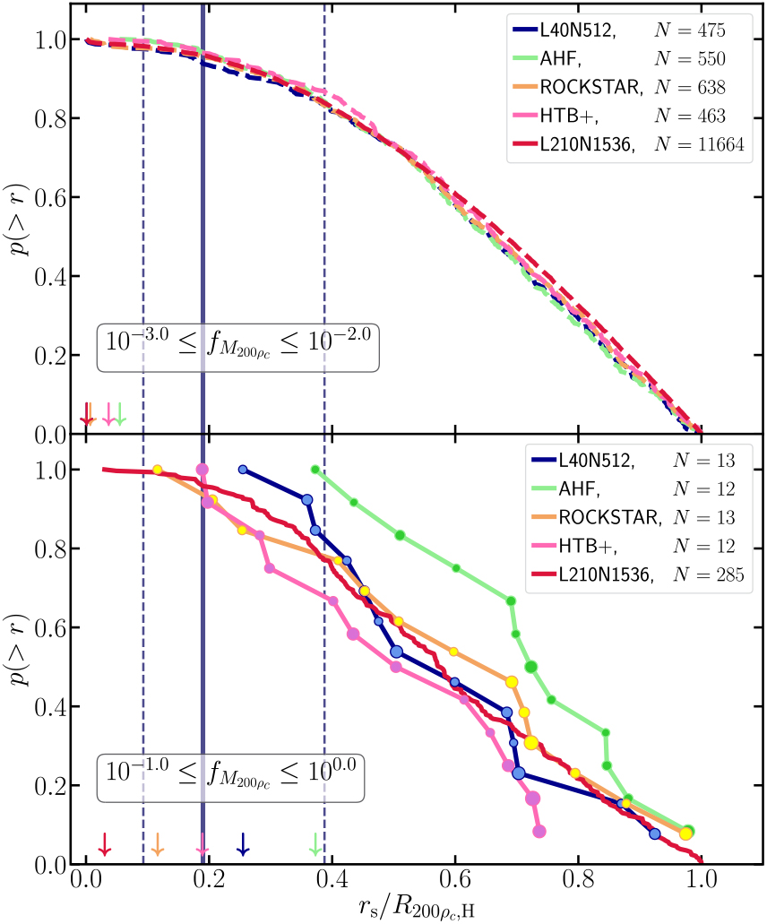
This trend is also seen in HBT+. By tracking 3DFOF halos, Han et al. (Reference Han, Cole, Frenk, Benitez-Llambay and Helly2018) found the inner regions of halos contain large subhalos that remain trapped due to dynamical friction. ROCKSTAR, another phase-space finder also reproduces the general trend.Footnote u In contrast, configuration-space-based finders like ahf shows a bias in the opposite direction in the very inner regions, and has no subhalos with f M200ρc ∼ 0.2 within ≳ 0.4R 200ρc.
To further investigate differences between codes, we compare the normalised cumulative radial distribution of subhalos in Figure 14 to further examine this apparent radial-mass dependence, focusing on low and high mass subhalos. Our lower mass bin samples halos composed of ∼100–1 000 particles for the smallest halos in this sample, well above the particle number threshold used to identify structures. Our upper mass bin effectively chooses major mergers. We find little difference between codes, with the inner most objects found well within the scale radius of the host halo. There is greater disagreement for large subhalos, in part owing to how the centre of a halo is defined (most bound particle, shrinking spheres estimate of mass, total bulk centre of mass). Nevertheless, we see that ahf is noticeably more biased to identifying large subhalos at larger radii that the other codes, a consequence of its configuration-space-based approach.
4. Discussion and conclusion
We have presented VELOCIraptor, a novel code designed to identify halos, subhalos, tidal debris and galaxies in both N-body and full hydrodynamical simulations using phase-space information. We have demonstrated that the code robustly identify (sub)halos, particularly cases that are typically notoriously diffi-cult for such codes, namely the mass reconstruction of subhalos deep inside their host halo and major mergers. We summarise key features/results below.
VELOCIraptor identifies structures in a multi-step process. For N-body simulations, it first identifies field halos using a 3DFOF followed by a 6DFOF algorithm. The next step identifies substructure in each halo in two stages. The first stage uses the previously developed algorithm described in Elahi et al. (Reference Elahi, Thacker and Widrow2011), finding velocity outliers (the so-called peaks above the Maxwellian sea) and linking particles using a phase-space FOF. The next stage is to find any remaining large minor/major mergers using an iterative search for dense phase-space cores that are then grown in an iterative fashion using phase-space tensors.
We find that 6DFOF objects are more representative of DM halos than 3DFOF objects as 3DFOF objects can link separate virialised overdensities together via particle bridges. The 6DFOF step separates early stage accretion/merger events, with the average number of 1.3 6DFOF objects per 3DFOF objects. The 6DFOF also removes outer unbound particles from the 3DFOF candidate, with FOF masses changing by M 6DFOF = 0.82M 3DFOF while leaving spherical overdensity masses, particularly 200ρc, unchanged.
The substructure algorithm (tested in Elahi et al. Reference Elahi, Thacker and Widrow2011, Reference Elahi2013, and shown to identify both subhalos and tidal debris) has the advantage over other algorithms of being able to identify subhalos deep within a host halo, where density contrasts relative to background are negligible. We highlighted a particular example where the average logarithmic density contrast between the subhalo and the host halo are ∼1, yet its particles are very distinct in velocity space. This subhalo does not undergo rapid artificial decrease in mass that affects most subhalo configuration-space-based finders.
The merger algorithm, a new addition to the code, is fully described here. This algorithm uses full phase-space tensors to assign particles to any phase-space dense cores that are not already tagged as substructure. This technique, inspired by rockstar (Behroozi et al. Reference Behroozi, Wechsler and Wu2013) and Gaussian mixture models, can separate substructures from the main halo deep within the host (at least up to the scale radius of a host halo). The use of phase-space tensors allows for the mass assignment scheme to asymmetric tidal features associated with an object, unlike ROCKSTAR, which uses a scalar dispersion to assign particles. The iterative growth is also more physical than assigning particles using Gaussian mixture models, which assume a global dispersion tensor. This method does not necessarily artificially shrink halos as they move towards pericentre, as seen in the example figures in the appendix, though the scheme can occasionally lose halos or result in mass fluctuations of a few when objects overlap significantly. This can be alleviated somewhat by using finer steps when searching for cores and assigning mass.
The resulting subhalo mass function reproduces the mass and radial distribution seen in codes that track particles, such as HBT+. Like this FOF tracker, the subhalo mass function can be decomposed into a distribution for low and high mass ratios. The low mass ratio end is described by a power-law with an exponential cut-off, with an index of $\alpha = \mathop {1.85}\nolimits_{ - 0.18}^{ + 0.16} $ , and a cut-off mass ratio scale of f o ∼ 0.05. Our simulation does not have enough halos to well constrain the high mass end it can either be characterised by a power-law with a much flatter slope or possibly a lognormal distribution in mass ratio.
Critically, VELOCIraptor can recover the radial-mass distribution seen in tracking codes like HBT+, with larger subhalos found at smaller radii, without the need of tracking.The central regions within the scale radius of a halo are dominated by large subhalos and merger remnants. Although our fiducial simulation only contains a small sample of ∼50 well-resolved halos composed of ≳105 particles, which is not enough to rigorously constrain the inner radial distribution, these halos are resolved enough for this trend to be observed by HBT+ and recovered by VELOCIraptor. This is in contrast to the distribution recovered by configuration-space-based finders. The code also does not introduce possibly spurious phase-space structures like rockstar, which also recovers the radial-mass dependence.
This radial-mass dependence is seen in our larger volume simulation, which contains ∼1 500 well-resolved halos, including ∼50 halos composed of 106 particles. As we do not analyse this simulation with HBT+, we cannot definitively say that the observed trend is that recovered by tracking, though given the results from our fiducial simulation, it is likely in agreement.
The code is in active development. New input interfaces for hydrodynamical simulations are being developed (e.g. Cañas et al. Reference Cañas, Elahi, Welker, Lagos, Power, Dubois and Pichon2018) and it is being incorporated into the swift Hydrodynamical N-body code (www.swiftsim.com Schaller et al. Reference Schaller, Gonnet, Chalk and Draper2016). Additional libraries are being integrated to improve the parallel efficiency, such as the ADIOS library, designed for parallel IO at the ∼104 node scale, and METIS for efficient MPI decomposition. The output produced also lends itself to large-scale processing as it produces compressed, self-describing binary HDF5 data.
Finally VELOCIraptor is not limited to analysing cosmological simulations. The primary substructure algorithm is suited to finding clustering in a variety of data. One novel application could be to decompose data from GAIA (Lindegren et al. Reference Lindegren2018), which contains five-dimensional phase-space information for 1.3 billion stars, and full 6D phase-space information for 7 million in the Milky Way. Early analysis shows that the mean velocity structure of the Milky Way disk is complex, with features indicative of substructure in the solar neighbourhood Gaia Collaboration et al. (Reference Collaboration2018). This data set is only just beginning to be mined for kinematic structures (e.g. Hawkins & Wyse Reference Hawkins and Wyse2018; Price-Whelan & Bonaca Reference Price-Whelan and Bonaca2018; Marchetti, Rossi, & Brown Reference Marchetti, Rossi and Brown2018). For instance, Castro-Ginard et al. (Reference Castro-Ginard, Jordi, Luri, Julbe, Morvan, Balaguer-Núñez and Cantat-Gaudin2018) used clustering algorithms and artificial neural networks to identify open clusters in the GAIA data set. This method essentially looks for full phase-space (configuration and velocity) clustering akin to a 6DFOF algorithm, as such is tailored to identifying open clusters. The nature of the substructure algorithm in VELOCIraptor makes it well suited for identifying open clusters and other substructures and even be extended to use other information, such as metallicity, making analysing this data with the code an interesting exercise.
Author ORCIDs
Pascal J. Elahi, https://orcid.org/0000-0002-6154-7224; Rhys J. J. Poulton, https://orcid.org/0000-0003-2049-520X; Chris Power, https://orcid.org/0000-0002-4003-0904.
Acknowledgements
The authors would like to thank the anonymous referee for insightful comments that helped improve the clarity of the text.
RC is supported by the SIRF awarded by the University of Western Australia Scholarships Committee, and the Consejo Nacional de Ciencia y Tecnología (CONACyT) scholarship No. 438594 and the MERAC Foundation. RP is supported by a University of Western Australia Scholarship. Parts of this research were conducted by the Australian Research Council Centre of Excellence for All Sky Astrophysics in 3 Dimensions (ASTRO 3D), through project number CE170100013. CL is funded by a Discovery Early Career Researcher Award DE150100618. CL also thanks the merac Foundation for a Postdoctoral Research Award.
The authors contributed to this paper in the following ways: PJE ran simulations and analysed the data, made the plots, and wrote the bulk of the paper. PJE is the primary developer of both VELOCIraptor. RC, RT, and JW designed and developed various aspects of the code: RC developed the core search; RT developed the compilation infrastructure; and JW bug tested and developed the interface with SWIFTSIM. RP, CL, CP, and AR assisted in the design of various aspects of the code. All authors have read and commented on the paper.
Facilities Magnus (Pawsey Supercomputing Centre)
Software
VELOCIraptor https://github.com/pelahi/VELOCIraptor-STF
TreeFrog https://github.com/pelahi/TreeFrog
Nbodylib https://github.com/pelahi/NBodylib
VELOCIraptor_PYTHON_TOOLS https://github.com/pelahi/VELOCIraptor_Python_Tools
MergerTreeDendograms https://github.com/rhyspoulton/MergerTree-Dendograms
ahf http://popia.ft.uam.es/AHF/Download.html
Rockstar https://bitbucket.org/gfcstanford/rockstar
HBT+ https://github.com/Kambrian/HBTplus
Additional Software Python, Matplotlib (Hunter Reference Hunter2007), Scipy (Jones et al. 01), Emcee (Foreman-Mackey et al. Reference Foreman-Mackey, Hogg, Lang and Goodman2013), Scikit (Pedregosa et al. Reference Pedregosa2011), and Gadget (Springel Reference Springel2005).
Appendix A. Orbits
We show the orbits of a low mass subhalo accreted at high redshift and large subhalo accreted at late times in Figure C.1. The poorly resolved subhalo is still recovered when deep inside the host halo even when composed of ∼30 particles. There are gaps in the subhalo’s orbit where it is momentarily lost. The large subhalo is accreted at late times and is still approaching pericentre. It does lose an appreciable amount of mass as it approaches pericentre, decreasing in mass by ∼20% over the last two snapshots as it moves from r/R 200ρ c = 0.65 to its current position of r/R 200ρ c = 0.41. For comparison, the configuration-space-based finder AHF shrinks the object by ∼2 over the same period.
Appendix B. Tables
We list the complete set of configuration options along with a list of properties calculated by VELOCIraptor.
VELOCIraptor configuration parameters.
VELOCIraptor Outputted halo/galaxy properties.

Appendix C. Associated tools
VELOCIraptor comes with a PYTHON-2/3 tool-kit, specifically routines to manipulate the output data produced by the various codes. Typically, these produce DICT containing NUMPY arrays, allowing for quick analysis and plotting. The repositories also come with examples of producing metric plots. The codes are PYTHON-3 (compatible with PYTHON-2) and make use of numpy, h5py, scipy, matplotlib, and scikit.learn.
Reconstructed subhalo orbital and evolution: we plot the orbital life of a poorly resolved subhalo found at r/R 200ρ = 0.15 (left) and a large-subhalo found at r/R 200ρ = 0.41. Similar to Figure 7.