


1 Introduction
The study of Prym curves from an algebraic perspective was initiated by Mumford in his seminal paper [Reference MumfordMum74]. Alongside Beauville’s work [Reference BeauvilleBea77], where he provides a modular interpretation of Prym curves, these contributions laid the foundation for the study of the moduli space of Prym curves. This is defined as
parametrizing pairs $(C, \eta )$
where C is a smooth curve of genus g and
$(C, \eta )$
where C is a smooth curve of genus g and $\eta $
is a
$\eta $
is a $2$
-torsion line bundle of C.
$2$
-torsion line bundle of C.
One natural question about $\mathcal {R}_g$
is computing its Kodaira dimension. This problem was the focus of several mathematicians, who described the geometry of
$\mathcal {R}_g$
is computing its Kodaira dimension. This problem was the focus of several mathematicians, who described the geometry of $\mathcal {R}_g$
for almost all values of g. This space is rational if
$\mathcal {R}_g$
for almost all values of g. This space is rational if $2\leq g \leq 4$
, see [Reference DolgachevDol85], [Reference CataneseCat83], unirational, if
$2\leq g \leq 4$
, see [Reference DolgachevDol85], [Reference CataneseCat83], unirational, if $5\leq g \leq 7$
, see [Reference Mori and MukaiMM83], [Reference DonagiDon84], [Reference VerraVer08], [Reference VerraVer84], [Reference Izadi, Lo Giudice and SankaranIGS08], [Reference Farkas and VerraFV16] uniruled if
$5\leq g \leq 7$
, see [Reference Mori and MukaiMM83], [Reference DonagiDon84], [Reference VerraVer08], [Reference VerraVer84], [Reference Izadi, Lo Giudice and SankaranIGS08], [Reference Farkas and VerraFV16] uniruled if $g = 8$
, see [Reference Farkas and VerraFV16] and of general type if
$g = 8$
, see [Reference Farkas and VerraFV16] and of general type if $g\geq 13, g \neq 16$
, see [Reference Farkas and LudwigFL10], [Reference BrunsBru16], [Reference Farkas, Jensen and PayneFJP24].
$g\geq 13, g \neq 16$
, see [Reference Farkas and LudwigFL10], [Reference BrunsBru16], [Reference Farkas, Jensen and PayneFJP24].
Through the natural map $\mathcal {P}_g\colon \mathcal {R}_g \rightarrow \mathcal {A}_{g-1}$
, one can relate the geometry of principally polarized Abelian varieties to the geometry of curves. For
$\mathcal {P}_g\colon \mathcal {R}_g \rightarrow \mathcal {A}_{g-1}$
, one can relate the geometry of principally polarized Abelian varieties to the geometry of curves. For $2\leq g \leq 6$
the map
$2\leq g \leq 6$
the map $\mathcal {P}_g$
is surjective, and hence the characterization above is fundamental in understanding the birational geometry of the moduli of Prym varieties.
$\mathcal {P}_g$
is surjective, and hence the characterization above is fundamental in understanding the birational geometry of the moduli of Prym varieties.
Similarly, we can consider the moduli space $\mathcal {R}_{g,2}$
parametrizing tuples
$\mathcal {R}_{g,2}$
parametrizing tuples $(C,x+y,\eta )$
where C is a smooth curve of genus g, the points x and y of C are distinct, and
$(C,x+y,\eta )$
where C is a smooth curve of genus g, the points x and y of C are distinct, and $\eta $
is a line bundle satisfying
$\eta $
is a line bundle satisfying $\eta ^{\otimes 2} \cong \mathcal {O}_C(-x-y)$
. This space comes equipped with a map
$\eta ^{\otimes 2} \cong \mathcal {O}_C(-x-y)$
. This space comes equipped with a map $\mathcal {P}_{g,2} \colon \mathcal {R}_{g,2} \rightarrow \mathcal {A}_g$
. This correspondence between pointed curves and principally polarized Abelian varieties motivates the study of the birational geometry of
$\mathcal {P}_{g,2} \colon \mathcal {R}_{g,2} \rightarrow \mathcal {A}_g$
. This correspondence between pointed curves and principally polarized Abelian varieties motivates the study of the birational geometry of $\mathcal {R}_{g,2}$
. We know that
$\mathcal {R}_{g,2}$
. We know that $\mathcal {R}_{g,2}$
is unirational for
$\mathcal {R}_{g,2}$
is unirational for $3\leq g \leq 5$
, uniruled for
$3\leq g \leq 5$
, uniruled for $g= 6$
and of general type if
$g= 6$
and of general type if $g \geq 16$
or
$g \geq 16$
or $ g = 13$
, see [Reference Lelli-Chiesa, Knutsen and VerraLCKV23], [Reference BudBud24] and [Reference Farkas, Jensen and PayneFJP24].
$ g = 13$
, see [Reference Lelli-Chiesa, Knutsen and VerraLCKV23], [Reference BudBud24] and [Reference Farkas, Jensen and PayneFJP24].
When studying the birational geometry of $\mathcal {M}_g$
, Brill-Noether Theory plays a fundamental role in showing that
$\mathcal {M}_g$
, Brill-Noether Theory plays a fundamental role in showing that $\mathcal {M}_g$
is of general type when
$\mathcal {M}_g$
is of general type when $g \geq 22$
, see [Reference Harris and MumfordHM82], [Reference HarrisHar84], [Reference Eisenbud and HarrisEH87] and [Reference Farkas, Jensen and PayneFJP20]. When
$g \geq 22$
, see [Reference Harris and MumfordHM82], [Reference HarrisHar84], [Reference Eisenbud and HarrisEH87] and [Reference Farkas, Jensen and PayneFJP20]. When $g\geq 24$
, we can consider numbers
$g\geq 24$
, we can consider numbers $r, d$
such that
$r, d$
such that ![]() and look at the locus of curves
and look at the locus of curves $[C] \in \mathcal {M}_g$
for which the Brill-Noether variety
$[C] \in \mathcal {M}_g$
for which the Brill-Noether variety $W^r_d(C)$
is nonempty. This locus is a divisor in
$W^r_d(C)$
is nonempty. This locus is a divisor in $\mathcal {M}_g$
and the class of its closure in
$\mathcal {M}_g$
and the class of its closure in $\overline {\mathcal {M}}_g$
can be used to show that
$\overline {\mathcal {M}}_g$
can be used to show that $\mathcal {M}_g$
is of general type when
$\mathcal {M}_g$
is of general type when $g\geq 24$
. For a Prym curve
$g\geq 24$
. For a Prym curve $[C,\eta ] \in \mathcal {R}_g$
we can consider
$[C,\eta ] \in \mathcal {R}_g$
we can consider $\pi \colon \widetilde {C} \rightarrow C$
the associated double cover and look at the locus
$\pi \colon \widetilde {C} \rightarrow C$
the associated double cover and look at the locus

where the norm map sends a line bundle $L \in \mathrm {Pic}(\widetilde {C})$
to
$L \in \mathrm {Pic}(\widetilde {C})$
to $\wedge ^2\pi _*L \otimes \eta $
. Equivalently, it sends a line bundle
$\wedge ^2\pi _*L \otimes \eta $
. Equivalently, it sends a line bundle $\mathcal {O}_{\widetilde {C}}(D)$
to
$\mathcal {O}_{\widetilde {C}}(D)$
to $\mathcal {O}_C(\pi _*D)$
for every divisor D on
$\mathcal {O}_C(\pi _*D)$
for every divisor D on $\widetilde {C}$
.
$\widetilde {C}$
.
These Prym-Brill-Noether loci can be understood as Brill-Noether loci on $\widetilde {C}$
that take into account the involution
$\widetilde {C}$
that take into account the involution $\iota \colon \widetilde {C} \rightarrow \widetilde {C}$
associated to the double cover
$\iota \colon \widetilde {C} \rightarrow \widetilde {C}$
associated to the double cover $\pi \colon \widetilde {C}\rightarrow C$
. These loci were introduced in [Reference WeltersWel85] to understand the singularities of Prym varieties, particularly by computing the expected dimension and describing the smooth locus of
$\pi \colon \widetilde {C}\rightarrow C$
. These loci were introduced in [Reference WeltersWel85] to understand the singularities of Prym varieties, particularly by computing the expected dimension and describing the smooth locus of $V^r(C,\eta )$
. Subsequently, it was shown that for a generic
$V^r(C,\eta )$
. Subsequently, it was shown that for a generic $(C,\eta )$
, the locus
$(C,\eta )$
, the locus $V^r(C,\eta )$
has the expected dimension, see [Reference BertramBer87], [Reference SchwarzSch17] and is irreducible when
$V^r(C,\eta )$
has the expected dimension, see [Reference BertramBer87], [Reference SchwarzSch17] and is irreducible when $g>\frac {r(r+1)}{2} + 1$
, see [Reference DebarreDeb00]. Viewing
$g>\frac {r(r+1)}{2} + 1$
, see [Reference DebarreDeb00]. Viewing $V^r(C,\eta )$
as a Lagrangian degeneracy locus, De Concini and Pragacz computed the virtual class of this locus in the Prym variety, see [Reference De Concini and PragaczDCP95].
$V^r(C,\eta )$
as a Lagrangian degeneracy locus, De Concini and Pragacz computed the virtual class of this locus in the Prym variety, see [Reference De Concini and PragaczDCP95].
In recent years, two perspectives on the study of Prym-Brill-Noether loci have arisen. On the one hand, the tropical geometry approach was used to provide another proof for the dimension estimate of $V^r(C,\eta )$
, along with many other properties, see [Reference Creech, Len, Ritter and WuCLRW20], [Reference Len and UlirschLU21], [Reference Jensen and PayneJP21] and the references therein. On the other hand, the moduli theory approach was used to understand the birational geometry of
$V^r(C,\eta )$
, along with many other properties, see [Reference Creech, Len, Ritter and WuCLRW20], [Reference Len and UlirschLU21], [Reference Jensen and PayneJP21] and the references therein. On the other hand, the moduli theory approach was used to understand the birational geometry of $\mathcal {R}_g$
for small values of g, see [Reference Farkas and VerraFV16]. Moreover, for
$\mathcal {R}_g$
for small values of g, see [Reference Farkas and VerraFV16]. Moreover, for $g = \frac {r(r+1)}{2} +1$
, it was shown in [Reference BudBud22a] that the universal Prym-Brill-Noether locus
$g = \frac {r(r+1)}{2} +1$
, it was shown in [Reference BudBud22a] that the universal Prym-Brill-Noether locus
has a unique irreducible component dominating $\mathcal {R}_g$
.
$\mathcal {R}_g$
.
For $r\geq 3$
and
$r\geq 3$
and $ g = \frac {r(r+1)}{2}$
we consider the locus
$ g = \frac {r(r+1)}{2}$
we consider the locus
It follows immediately from [Reference Fulton and LazarsfeldFL81, Theorem II], [Reference DebarreDeb00, Example 1.4] and [Reference SteffenSte98, Theorem 2.9] that in this case $\mathcal {R}^r_g$
is a divisor in
$\mathcal {R}^r_g$
is a divisor in $\mathcal {R}_g$
. The main goal of this paper is to compute the class of the Prym-Brill-Noether divisor
$\mathcal {R}_g$
. The main goal of this paper is to compute the class of the Prym-Brill-Noether divisor $\overline {\mathcal {R}}^r_g$
in
$\overline {\mathcal {R}}^r_g$
in $\mathrm {Pic}_{\mathbb {Q}}(\overline {\mathcal {R}}_g)$
, where the closure
$\mathrm {Pic}_{\mathbb {Q}}(\overline {\mathcal {R}}_g)$
, where the closure $\overline {\mathcal {R}}_g$
is described in [Reference Ballico, Casagrande and FontanariBCF04] and [Reference Farkas and LudwigFL10]. Our main result is:
$\overline {\mathcal {R}}_g$
is described in [Reference Ballico, Casagrande and FontanariBCF04] and [Reference Farkas and LudwigFL10]. Our main result is:
Theorem 1.1. Let $r \geq 3 $
and
$r \geq 3 $
and $g = \frac {r(r+1)}{2}$
. Then the class of
$g = \frac {r(r+1)}{2}$
. Then the class of $\overline {\mathcal {R}}^r_g$
in
$\overline {\mathcal {R}}^r_g$
in $\mathrm {Pic}_{\mathbb {Q}}(\overline {\mathcal {R}}_g)$
is equal to
$\mathrm {Pic}_{\mathbb {Q}}(\overline {\mathcal {R}}_g)$
is equal to
 $$\begin{align*}[\overline{\mathcal{R}}^r_g] = c\cdot \left(a\lambda- b_0'\delta_0' - b_0"\delta_0"-b_0^{\mathrm{ram}}\delta_0^{\mathrm{ram}}- \sum_{i=1}^{g-1}b_i\delta_i - \sum_{i = 1}^{[\frac{g}{2}]}b_{i:g-i}\delta_{i:g-i}\right) \end{align*}$$
where $a = g+1$
,
$a = g+1$
, $b_0' = \frac {g}{6}$
,
$b_0' = \frac {g}{6}$
, $b_0^{\mathrm {ram}} = \frac {g}{4}$
,
$b_0^{\mathrm {ram}} = \frac {g}{4}$
, $b_0" = \frac {g^2-g+2}{8}$
and
$b_0" = \frac {g^2-g+2}{8}$
and $b_i = \frac {(g-i)(g+i-1)}{2}$
.
$b_i = \frac {(g-i)(g+i-1)}{2}$
.
The constants c and $b_{i:g-i}$
were not determined.
$b_{i:g-i}$
were not determined.
Theorem 1.1 provides another proof of the fact that $\mathcal {R}_{15}$
is of general type, proven in [Reference BrunsBru16]. Moreover, by pulling back this divisor to
$\mathcal {R}_{15}$
is of general type, proven in [Reference BrunsBru16]. Moreover, by pulling back this divisor to $\mathcal {R}_{14,2}$
we are able to prove that
$\mathcal {R}_{14,2}$
we are able to prove that
Theorem 1.2. The moduli space $\mathcal {R}_{14,2}$
is of general type.
$\mathcal {R}_{14,2}$
is of general type.
Using the numerology of Theorem 1.1, we can intersect the Prym-Brill-Noether divisor with a pencil of Prym curves on a Nikulin surface. Because the intersection number is negative, we obtain the following result about the Nikulin locus (i.e. the locus of Prym curves lying on Nikulin surfaces) in $\mathcal {R}_g$
:
$\mathcal {R}_g$
:
Corollary 1.3. Let $r\geq 3$
and
$r\geq 3$
and $g = \frac {r(r+1)}{2}$
. Then the Nikulin locus is contained in the Prym-Brill-Noether divisor.
$g = \frac {r(r+1)}{2}$
. Then the Nikulin locus is contained in the Prym-Brill-Noether divisor.
This is another proof that Prym-Brill-Noether varieties do not have the expected dimension on Prym curves in the Nikulin locus. A more general version of this result, proved using the geometry of Nikulin surfaces in an essential way, appears in [Reference D’Evanghelista and Lelli-ChiesaDLC23].
In order to prove Theorem 1.1, we will consider the intersection of $\overline {\mathcal {R}}^r_g$
with the boundary divisor
$\overline {\mathcal {R}}^r_g$
with the boundary divisor $\Delta ^{\prime \prime }_0$
. To understand this intersection we will work with Prym limit linear series for curves that are not of compact type. The theory developed by Osserman in [Reference OssermanOss16] and [Reference OssermanOss19] is well-suited to tackle this problem. The norm condition on the limit linear series will substantially simplify the situation. To compute the class of
$\Delta ^{\prime \prime }_0$
. To understand this intersection we will work with Prym limit linear series for curves that are not of compact type. The theory developed by Osserman in [Reference OssermanOss16] and [Reference OssermanOss19] is well-suited to tackle this problem. The norm condition on the limit linear series will substantially simplify the situation. To compute the class of $\overline {\mathcal {R}}^r_g$
, we will have to compute the class of a strongly Brill-Noether divisor in
$\overline {\mathcal {R}}^r_g$
, we will have to compute the class of a strongly Brill-Noether divisor in $\overline {\mathcal {M}}_{g-1,2}$
.
$\overline {\mathcal {M}}_{g-1,2}$
.
For two points $x,y$
on a curve C, we consider the sequence
$x,y$
on a curve C, we consider the sequence $D_\bullet (x,y)$
of effective divisors:
$D_\bullet (x,y)$
of effective divisors:
 $$\begin{align*}0 \leq x+y \leq 2\cdot(x+y) \leq \cdots \leq n\cdot (x+y) \leq \cdots\end{align*}$$
and the multivanishing sequence $\textbf {a}$
:
$\textbf {a}$
:
 $$\begin{align*}a_0 = 0 \leq a_1 = 2 \leq a_2 = 4 \leq \cdots \leq a_r = 2r \end{align*}$$
For $r \geq 3$
and
$r \geq 3$
and $ g = \frac {r(r+1)}{2} - 1$
, we consider the locus in
$ g = \frac {r(r+1)}{2} - 1$
, we consider the locus in $\mathcal {M}_{g,2}$
of pointed curves
$\mathcal {M}_{g,2}$
of pointed curves $[C, x, y]$
satisfying that C admits a
$[C, x, y]$
satisfying that C admits a $g^r_{g+r}$
with multivanishing sequence
$g^r_{g+r}$
with multivanishing sequence $\textbf {a}$
along
$\textbf {a}$
along $D_\bullet (x,y)$
. That is:
$D_\bullet (x,y)$
. That is:

This locus has a divisorial component and we can show
Theorem 1.4. In the notation above, the strongly Brill-Noether divisor is irreducible and its class satisfies:
 $$\begin{align*}[\overline{\mathcal{M}}^r_{g, g+r}\left(D_\bullet, \textbf{a}\right)] = c\cdot\left(a_1\psi_1 + a_2\psi_2 + a\lambda - b_0\delta_0 - \sum_{i=0}^{g-1} b_{i, \left\{1,2\right\}}\delta_{i, \left\{1,2\right\}} - \sum_{i=1}^{g-1}b_{i,1}\delta_{i,1}\right) \end{align*}$$
where $a_1 = a_2 = \frac {g^2+g+2}{8}$
,
$a_1 = a_2 = \frac {g^2+g+2}{8}$
, $a = g+2$
,
$a = g+2$
, $b_0 = \frac {g+1}{6}$
,
$b_0 = \frac {g+1}{6}$
, $b_{i,\left \{1,2\right \}} = \frac {(g-i)(g+i+1)}{2}$
and
$b_{i,\left \{1,2\right \}} = \frac {(g-i)(g+i+1)}{2}$
and $c = \frac {(g+1)!}{g-1}\cdot 2^{g-1}\prod _{i=1}^{r}\frac {i!}{(2i)!}$
.
$c = \frac {(g+1)!}{g-1}\cdot 2^{g-1}\prod _{i=1}^{r}\frac {i!}{(2i)!}$
.
The coefficients $b_{i,1}$
for
$b_{i,1}$
for $1\leq i \leq g-1$
were not determined.
$1\leq i \leq g-1$
were not determined.
In order to prove Theorem 1.1, several basic Brill-Noether properties will be required. We provide these results in Section 2. Next, we consider in Section 3, the intersection of the divisor $\overline {\mathcal {R}}^r_g$
with several test curves. The interplay between the norm condition, the Brill-Noether number and limit linear series is first investigated in this section. In Section 4, we consider different pullbacks of the divisor
$\overline {\mathcal {R}}^r_g$
with several test curves. The interplay between the norm condition, the Brill-Noether number and limit linear series is first investigated in this section. In Section 4, we consider different pullbacks of the divisor $\overline {\mathcal {R}}^r_g$
. These pullbacks consist of a unique non-boundary divisor and hence, will provide new relations between the coefficients of the class
$\overline {\mathcal {R}}^r_g$
. These pullbacks consist of a unique non-boundary divisor and hence, will provide new relations between the coefficients of the class $[\overline {\mathcal {R}}^r_g]$
in
$[\overline {\mathcal {R}}^r_g]$
in $\mathrm {Pic}_{\mathbb {Q}}(\overline {\mathcal {R}}_g)$
. The results in Section 3 and Section 4 conclude Theorem 1.1 and Theorem 1.2. Finally in Section 5 we deal with strongly Brill-Noether divisors in
$\mathrm {Pic}_{\mathbb {Q}}(\overline {\mathcal {R}}_g)$
. The results in Section 3 and Section 4 conclude Theorem 1.1 and Theorem 1.2. Finally in Section 5 we deal with strongly Brill-Noether divisors in $\overline {\mathcal {M}}_{g,2}$
. For a generic curve
$\overline {\mathcal {M}}_{g,2}$
. For a generic curve $[C]\in \mathcal {M}_g$
, the fibre of the strongly Brill-Noether divisor appearing in Theorem 1.4 is one-dimensional above
$[C]\in \mathcal {M}_g$
, the fibre of the strongly Brill-Noether divisor appearing in Theorem 1.4 is one-dimensional above $[C]$
. We consider the locus of tuples
$[C]$
. We consider the locus of tuples $(x,y, L)$
satisfying
$(x,y, L)$
satisfying $[C,x,y] \in \overline {\mathcal {M}}^r_{g, g+r}\left(D_{\bullet }, \textbf {a}\right)$
,
$[C,x,y] \in \overline {\mathcal {M}}^r_{g, g+r}\left(D_{\bullet }, \textbf {a}\right)$
, $L\in \mathrm {Pic}^{g+r}(C)$
and respecting the condition in the definition of
$L\in \mathrm {Pic}^{g+r}(C)$
and respecting the condition in the definition of $\overline {\mathcal {M}}^r_{g, g+r}\left(D_{\bullet }, \textbf {a}\right)$
. This is a one-dimensional locus in the product space
$\overline {\mathcal {M}}^r_{g, g+r}\left(D_{\bullet }, \textbf {a}\right)$
. This is a one-dimensional locus in the product space $C\times C \times \mathrm {Pic}^{g+r}(C)$
and can be realized as a flag degeneracy locus. We use the Fulton-Pragacz determinantal formula to compute the intersection of this locus with the divisors
$C\times C \times \mathrm {Pic}^{g+r}(C)$
and can be realized as a flag degeneracy locus. We use the Fulton-Pragacz determinantal formula to compute the intersection of this locus with the divisors $\Delta \times \mathrm {Pic}^{g+r}(C)$
and
$\Delta \times \mathrm {Pic}^{g+r}(C)$
and $C\times \left \{p\right \} \times \mathrm {Pic}^{g+r}(C)$
. This gives us the irreducibility, together with a relation between its coefficients in
$C\times \left \{p\right \} \times \mathrm {Pic}^{g+r}(C)$
. This gives us the irreducibility, together with a relation between its coefficients in $\mathrm {Pic}_{\mathbb {Q}}(\overline {\mathcal {M}}_{g,2})$
that will allow us to compute the coefficients of
$\mathrm {Pic}_{\mathbb {Q}}(\overline {\mathcal {M}}_{g,2})$
that will allow us to compute the coefficients of $\psi _1$
and
$\psi _1$
and $\psi _2$
. The intersection of
$\psi _2$
. The intersection of $\overline {\mathcal {M}}^r_{g, g+r}\left(D_{\bullet }, \textbf {a}\right)$
with the boundary divisor
$\overline {\mathcal {M}}^r_{g, g+r}\left(D_{\bullet }, \textbf {a}\right)$
with the boundary divisor $\Delta _{0,\left \{1,2\right \}}$
is easy to understand and will be used to conclude Theorem 1.4.
$\Delta _{0,\left \{1,2\right \}}$
is easy to understand and will be used to conclude Theorem 1.4.
2 Some basic Brill-Noether properties
To understand the intersection of $\overline {\mathcal {R}}^r_g$
with different divisors, we will require several well-known Brill-Noether properties, that we will recall in this section. We start by reviewing some basic definitions about linear series.
$\overline {\mathcal {R}}^r_g$
with different divisors, we will require several well-known Brill-Noether properties, that we will recall in this section. We start by reviewing some basic definitions about linear series.
In their seminal work on Brill–Noether Theory (see [Reference Eisenbud and HarrisEH86]), Eisenbud and Harris wanted to study line bundles of a given degree possessing numerous global sections. To accomplish this, they used the concept of a linear series:
Definition 2.1. Let C be a smooth curve of genus g. A linear series $g^r_d$
on X is a pair
$g^r_d$
on X is a pair $l = (L, V)$
where
$l = (L, V)$
where $L \in \mathrm {Pic}^d(C)$
is a degree d line bundle and
$L \in \mathrm {Pic}^d(C)$
is a degree d line bundle and $V\subseteq H^0(C,L)$
is an
$V\subseteq H^0(C,L)$
is an $(r+1)$
-dimensional subspace of the space of global sections on L. The variety parametrizing all
$(r+1)$
-dimensional subspace of the space of global sections on L. The variety parametrizing all $g^r_d$
’s on a curve C is denoted
$g^r_d$
’s on a curve C is denoted $G^r_d(C)$
Having some points $x_1, \ldots , x_n$
on C, it is natural to look at their vanishing orders with respect to linear series.
$x_1, \ldots , x_n$
on C, it is natural to look at their vanishing orders with respect to linear series.
Definition 2.2. Let $\textbf {a}$
be a sequence
$\textbf {a}$
be a sequence $0\leq a_0< \cdots < a_r \leq d$
. We say that a
$0\leq a_0< \cdots < a_r \leq d$
. We say that a $g^r_d$
, denoted
$g^r_d$
, denoted $(V,L)$
, has vanishing orders given by
$(V,L)$
, has vanishing orders given by $\textbf {a}$
at a point x if there exists a basis of V such that the vanishing orders at x of that basis are the
$\textbf {a}$
at a point x if there exists a basis of V such that the vanishing orders at x of that basis are the $a_i$
’s for
$a_i$
’s for $0\leq i \leq r$
.
$0\leq i \leq r$
.
If $\textbf {a}^1, \ldots , \textbf {a}^n$
are ramification profiles, we define the Brill-Noether number to be
$\textbf {a}^1, \ldots , \textbf {a}^n$
are ramification profiles, we define the Brill-Noether number to be
 $$\begin{align*}\rho(g,r,d,\textbf{a}^1,\ldots,\textbf{a}^n) = g-(r+1)(g-d+r)- \sum_{j=1}^{n}\sum_{i=0}^{r}a^j_i + n\cdot \frac{r(r+1)}{2}\end{align*}$$
The main result of [Reference Eisenbud and HarrisEH86] is a partial compactification of the space of linear series to curves that are of compact type. For a definition of limit linear series, we refer the reader to [Reference Eisenbud and HarrisEH86].
We have the following results, compiled from [Reference Eisenbud and HarrisEH87, Theorem 1.1] and [Reference FarkasFar00, Proposition 1.4.1].
Lemma 2.3. On a genus g curve, we consider limit linear $g^r_d$
’s having vanishing profiles
$g^r_d$
’s having vanishing profiles $\textbf {a}^1, \ldots , \textbf {a}^n$
at n marked points. Then we have the following:
$\textbf {a}^1, \ldots , \textbf {a}^n$
at n marked points. Then we have the following:
I) If $g=0$
and
$g=0$
and $[R,x_1,\ldots ,x_n] \in \overline {\mathcal {M}}_{0,n}$
admits such a limit
$[R,x_1,\ldots ,x_n] \in \overline {\mathcal {M}}_{0,n}$
admits such a limit $g^r_d$
, then the Brill-Noether number is positive, i.e:
$g^r_d$
, then the Brill-Noether number is positive, i.e:
 $$\begin{align*}\rho(0,r,d,\textbf{a}^1,\ldots,\textbf{a}^n) \geq 0\end{align*}$$
II) If $g=1, n=1$
and
$g=1, n=1$
and $[E,x] \in \overline {\mathcal {M}}_{1,1}$
admits such a
$[E,x] \in \overline {\mathcal {M}}_{1,1}$
admits such a $g^r_d$
, then
$g^r_d$
, then
 $$\begin{align*}\rho(1,r,d,\textbf{a}) \geq 0\end{align*}$$
III) If $g=1, n=2$
and
$g=1, n=2$
and $[E,x,y] \in \overline {\mathcal {M}}_{1,2}$
admits such a
$[E,x,y] \in \overline {\mathcal {M}}_{1,2}$
admits such a $g_d^r$
, then
$g_d^r$
, then
 $$\begin{align*}\rho(1,r,d,\textbf{a}^1, \textbf{a}^2) \geq -r\end{align*}$$
IV) Let $\mathcal {W} \subseteq \mathcal {M}_{2,1}$
be the Weierstrass divisor. If
$\mathcal {W} \subseteq \mathcal {M}_{2,1}$
be the Weierstrass divisor. If $g=2, n= 1$
and
$g=2, n= 1$
and $[C,x] \in \mathcal {M}_{2,1}\setminus \mathcal {W}$
admits such a
$[C,x] \in \mathcal {M}_{2,1}\setminus \mathcal {W}$
admits such a $g^r_d$
, we have:
$g^r_d$
, we have:
 $$\begin{align*}\rho(2,r,d,\textbf{a}) \geq 0\end{align*}$$
V) If $g=2, n =1 $
and
$g=2, n =1 $
and $[C,x] \in \partial \overline {\mathcal {M}}_{2,1}$
is a generic point of a boundary component admitting such a limit
$[C,x] \in \partial \overline {\mathcal {M}}_{2,1}$
is a generic point of a boundary component admitting such a limit $g^r_d$
, then:
$g^r_d$
, then:
 $$\begin{align*}\rho(2,r,d,\textbf{a}) \geq 0 \end{align*}$$
VI) If $[C,x_1,\ldots , x_n] \in \mathcal {M}_{g,n}$
is generic and admits such a
$[C,x_1,\ldots , x_n] \in \mathcal {M}_{g,n}$
is generic and admits such a $g^r_d$
, then
$g^r_d$
, then
 $$\begin{align*}\rho(g,r,d,\textbf{a}^1,\ldots,\textbf{a}^n) \geq 0\end{align*}$$
Our next goal is to understand the Brill-Noether theory of Prym curves. For this, we provide a pointed version of the main result in [Reference SchwarzSch17]. As in [Reference BudBud24], we denote by ![]() the moduli space parametrizing tuples
the moduli space parametrizing tuples $[C,x_1,\ldots ,x_n, \eta ]$
where
$[C,x_1,\ldots ,x_n, \eta ]$
where $[C, \eta ] \in \mathcal {R}_g$
and
$[C, \eta ] \in \mathcal {R}_g$
and $x_1, \ldots , x_n \in C$
. We have:
$x_1, \ldots , x_n \in C$
. We have:
Proposition 2.4. For a generic pointed Prym curve $[C,x,\eta ] \in \mathcal {C}^1\mathcal {R}_g$
, let
$[C,x,\eta ] \in \mathcal {C}^1\mathcal {R}_g$
, let $\widetilde {C}\rightarrow C$
be the associated double cover and let
$\widetilde {C}\rightarrow C$
be the associated double cover and let $\widetilde {x}_1,\widetilde {x}_2 \in \widetilde {C}$
be the two points in the preimage of x.
$\widetilde {x}_1,\widetilde {x}_2 \in \widetilde {C}$
be the two points in the preimage of x.
We consider some integers $r, d$
and some vanishing profiles
$r, d$
and some vanishing profiles $\textbf {a}^1, \textbf {a}^2$
such that the condition
$\textbf {a}^1, \textbf {a}^2$
such that the condition
 $$\begin{align*}\rho(g,r,d,\textbf{a}^1, \textbf{a}^2) <-r\end{align*}$$
is satisfied. Then $\widetilde {C}$
does not admit a
$\widetilde {C}$
does not admit a $g^r_d$
with ramification profiles
$g^r_d$
with ramification profiles $\textbf {a}^1$
and
$\textbf {a}^1$
and $\textbf {a}^2$
at
$\textbf {a}^2$
at $\widetilde {x}_1,\widetilde {x}_2$
.
$\widetilde {x}_1,\widetilde {x}_2$
.
Proof. We consider the map $\chi ^1_g\colon \mathcal {C}^1\mathcal {R}_g \rightarrow \mathcal {M}_{2g-1,2/S_2}$
sending
$\chi ^1_g\colon \mathcal {C}^1\mathcal {R}_g \rightarrow \mathcal {M}_{2g-1,2/S_2}$
sending $[C,x,\eta ]$
to
$[C,x,\eta ]$
to $[\widetilde {C},\widetilde {x}_1+\widetilde {x}_2]$
. This map can be extended to a map
$[\widetilde {C},\widetilde {x}_1+\widetilde {x}_2]$
. This map can be extended to a map
 $$\begin{align*}\chi^1_g\colon \overline{\mathcal{C}^1\mathcal{R}}_g\rightarrow \overline{\mathcal{M}}_{2g-1,2/S_2} \end{align*}$$
where the compactification of $\mathcal {C}^1\mathcal {R}_g$
is as in [Reference BudBud24, Section 6]. We consider
$\mathcal {C}^1\mathcal {R}_g$
is as in [Reference BudBud24, Section 6]. We consider $[X\cup _{y\sim p}E, x, \mathcal {O}_X, \eta _E]$
a generic point in the boundary divisor
$[X\cup _{y\sim p}E, x, \mathcal {O}_X, \eta _E]$
a generic point in the boundary divisor $\Delta _1$
of
$\Delta _1$
of $\overline {\mathcal {C}^1\mathcal {R}}_g$
. The image of this point through
$\overline {\mathcal {C}^1\mathcal {R}}_g$
. The image of this point through $\chi _g$
is
$\chi _g$
is $[X_1\cup _{y_1\sim p_1} \widetilde {E} \cup _{p_2\sim y_2} X_2, x_1, x_2]$
where
$[X_1\cup _{y_1\sim p_1} \widetilde {E} \cup _{p_2\sim y_2} X_2, x_1, x_2]$
where $[X_1, x_1, y_1]$
and
$[X_1, x_1, y_1]$
and $[X_2, x_2, y_2]$
are two copies of the generic curve
$[X_2, x_2, y_2]$
are two copies of the generic curve $[X,x,y] \in \mathcal {M}_{g-1,2}$
and
$[X,x,y] \in \mathcal {M}_{g-1,2}$
and $[\widetilde {E},p_1,p_2]$
is the associated double cover of
$[\widetilde {E},p_1,p_2]$
is the associated double cover of $[E,p,\eta _E]$
, that is
$[E,p,\eta _E]$
, that is $p_1$
and
$p_1$
and $p_2$
are the points in the preimage of p for the associated double cover.
$p_2$
are the points in the preimage of p for the associated double cover.
If we assume the proposition to be false, we get that $[X_1\cup _{y_1\sim p_1} \widetilde {E} \cup _{p_2\sim y_2} X_2, x_1, x_2]$
admits a limit
$[X_1\cup _{y_1\sim p_1} \widetilde {E} \cup _{p_2\sim y_2} X_2, x_1, x_2]$
admits a limit $g^r_d$
having ramification profiles
$g^r_d$
having ramification profiles $\textbf {a}^1$
and
$\textbf {a}^1$
and $\textbf {a}^2$
at
$\textbf {a}^2$
at $x_1$
and
$x_1$
and $x_2$
. We denote by
$x_2$
. We denote by $l_1, l_2$
and
$l_1, l_2$
and $l_{\widetilde {E}}$
the aspects of this limit linear series.
$l_{\widetilde {E}}$
the aspects of this limit linear series.
Using the additivity of the Brill-Noether numbers, see [Reference Eisenbud and HarrisEH86, Proposition 4.6], together with III and VI of Lemma 2.3, we obtain the contradiction
 $$\begin{align*}-r>\rho(g,r,d,\textbf{a}^1,\textbf{a}^2) \geq \rho(l_1,x_1,y_1) + \rho(l_2,x_2,y_2) + \rho(l_{\widetilde{E}},p_1,p_2) \geq 0+0+(-r) = -r.\end{align*}$$
To understand how Prym-Brill-Noether loci degenerate to the boundary component $\Delta _0"$
, we will require the study of multivanishing orders (with respect to a chain of divisors).
$\Delta _0"$
, we will require the study of multivanishing orders (with respect to a chain of divisors).
Definition 2.5. Let $l = (L, V)$
be a
$l = (L, V)$
be a $g^r_d$
on C and let
$g^r_d$
on C and let $\textbf {D}$
be a chain of effective divisors on C:
$\textbf {D}$
be a chain of effective divisors on C:
 $$\begin{align*}0 = D_0 < D_1 <\cdots < D_k \end{align*}$$
satisfying $\deg (D_k)> d$
. We say that a section
$\deg (D_k)> d$
. We say that a section $s \in V$
has multivanishing order
$s \in V$
has multivanishing order $\deg (D_i)$
with respect to
$\deg (D_i)$
with respect to $\textbf {D}$
if
$\textbf {D}$
if
 $$\begin{align*}s \in V\cap H^0(C,L-D_i) \ \mathrm{and} \ s \not\in V\cap H^0(C,L-D_{i+1}). \end{align*}$$
As before, there are exactly $r+1$
multivanishing orders, giving a multivanishing sequence
$r+1$
multivanishing orders, giving a multivanishing sequence
 $$\begin{align*}a^{\ell} (\textbf{D}): 0\leq a_0^{\ell}(\textbf{D}) < a_1^{\ell}(\textbf{D})\cdots < a_r^{\ell}(\textbf{D}) \leq d\end{align*}$$
with respect to $\textbf {D}$
.
$\textbf {D}$
.
Notice that in this situation, there can exist multiple independent sections having the same multivanishing order $\deg (D_i)$
. In fact, there can exist at most
$\deg (D_i)$
. In fact, there can exist at most $\deg (D_{i+1}) - \deg (D_i)$
such sections.
$\deg (D_{i+1}) - \deg (D_i)$
such sections.
Let $\textbf {a}$
be a sequence
$\textbf {a}$
be a sequence $0\leq a_0 \leq a_1\leq \cdots \leq a_r \leq d$
and let
$0\leq a_0 \leq a_1\leq \cdots \leq a_r \leq d$
and let $r_i$
be the number of times that i appears in this sequence. In this case, the Brill-Noether number is defined as
$r_i$
be the number of times that i appears in this sequence. In this case, the Brill-Noether number is defined as
 $$\begin{align*}\rho(g,r,d,\textbf{a}) = g-(r+1)(g-d+r)- \sum_{j=1}^{n}\sum_{i=0}^{r}a_i + \cdot \frac{r(r+1)}{2} - \sum_{i=0}^d \binom{r_i}{2}.\end{align*}$$
This number represents the expected dimension for the variety parametrizing $g^r_d$
’s with multivanishing orders
$g^r_d$
’s with multivanishing orders $\textbf {a}$
with respect to a chain of divisors
$\textbf {a}$
with respect to a chain of divisors $\textbf {D}$
. When this number is negative, a generic pointed curve does not admit such
$\textbf {D}$
. When this number is negative, a generic pointed curve does not admit such $g^r_d$
’s, see [Reference OssermanOss19]. If all the Brill-Noether varieties of
$g^r_d$
’s, see [Reference OssermanOss19]. If all the Brill-Noether varieties of $g^r_d$
’s respecting a multivanishing condition are of expected dimension for a pointed curve
$g^r_d$
’s respecting a multivanishing condition are of expected dimension for a pointed curve $[C, x_1,\ldots , x_n]$
we call the pointed curve strongly Brill-Noether general.
$[C, x_1,\ldots , x_n]$
we call the pointed curve strongly Brill-Noether general.
3 Intersection with test curves
A standard way of obtaining relations between the coefficients of a divisor is to intersect it with different test curves. One way to obtain test curves on the moduli space $\overline {\mathcal {R}}_g$
is to pull back known test curves in
$\overline {\mathcal {R}}_g$
is to pull back known test curves in $\overline {\mathcal {M}}_g$
. This approach was already employed in [Reference Farkas and LudwigFL10], [Reference PérezPér21], [Reference BudBud21] and [Reference BudBud22b]. We start by defining the test curves we will use in this section.
$\overline {\mathcal {M}}_g$
. This approach was already employed in [Reference Farkas and LudwigFL10], [Reference PérezPér21], [Reference BudBud21] and [Reference BudBud22b]. We start by defining the test curves we will use in this section.
Let $[X,p]$
be a generic genus
$[X,p]$
be a generic genus $g-1$
pointed curve. The test curve A in
$g-1$
pointed curve. The test curve A in $\overline {\mathcal {M}}_g$
is obtained by glueing at the point p an elliptic pencil along a base point. Pulling back the test curve A to
$\overline {\mathcal {M}}_g$
is obtained by glueing at the point p an elliptic pencil along a base point. Pulling back the test curve A to $\overline {\mathcal {R}}_g$
we obtain three test curves
$\overline {\mathcal {R}}_g$
we obtain three test curves $A_1$
,
$A_1$
, $A_{g-1}$
and
$A_{g-1}$
and $A_{1:g-1}$
contained in the boundary divisors
$A_{1:g-1}$
contained in the boundary divisors $\Delta _1$
,
$\Delta _1$
, $\Delta _{g-1}$
and
$\Delta _{g-1}$
and $\Delta _{1:g-1}$
respectively.
$\Delta _{1:g-1}$
respectively.
Let $g = \frac {r(r+1)}{2}$
and
$g = \frac {r(r+1)}{2}$
and $\mathcal {R}_g^r$
the locus parametrizing curves
$\mathcal {R}_g^r$
the locus parametrizing curves $[C,\eta ]$
for which
$[C,\eta ]$
for which $V^r(C,\eta )$
is non-empty. We denote by
$V^r(C,\eta )$
is non-empty. We denote by $\overline {\mathcal {R}}^r_g$
the closure of this locus in
$\overline {\mathcal {R}}^r_g$
the closure of this locus in $\overline {\mathcal {R}}_g$
. We consider the map
$\overline {\mathcal {R}}_g$
. We consider the map $\chi _g\colon \overline {\mathcal {R}}_g \rightarrow \overline {\mathcal {M}}_{2g-1}$
sending a Prym curve
$\chi _g\colon \overline {\mathcal {R}}_g \rightarrow \overline {\mathcal {M}}_{2g-1}$
sending a Prym curve $[C,\eta ]$
to the associated double cover
$[C,\eta ]$
to the associated double cover $\widetilde {C}$
of C. Using this map, we prove:
$\widetilde {C}$
of C. Using this map, we prove:
Proposition 3.1. We have the intersection number $A_{g-1} \cdot \overline {\mathcal {R}}_g^r = 0$
.
$A_{g-1} \cdot \overline {\mathcal {R}}_g^r = 0$
.
Proof. By definition, we have that $\overline {\mathcal {R}}^r_g \subseteq \chi _g^{-1}(\overline {\mathcal {M}}_{2g-1,2g-2}^r)$
. To conclude our proposition, it is enough to show that the curves in
$\overline {\mathcal {R}}^r_g \subseteq \chi _g^{-1}(\overline {\mathcal {M}}_{2g-1,2g-2}^r)$
. To conclude our proposition, it is enough to show that the curves in $\chi _g(A_{g-1})$
do not admit any limit
$\chi _g(A_{g-1})$
do not admit any limit $g^r_{2g-2}$
.
$g^r_{2g-2}$
.
The fact that $\chi _g(A_{g-1})$
and
$\chi _g(A_{g-1})$
and $\overline {\mathcal {M}}_{2g-1,2g-2}^r$
do not intersect follows from Proposition 2.4 and part II of Lemma 2.3. The conclusion follows from the additivity of Brill-Noether numbers.
$\overline {\mathcal {M}}_{2g-1,2g-2}^r$
do not intersect follows from Proposition 2.4 and part II of Lemma 2.3. The conclusion follows from the additivity of Brill-Noether numbers.
We also have that the test curve $A_1$
and the divisor
$A_1$
and the divisor $\overline {\mathcal {R}}^r_g$
do not intersect. However, the proof is more involved due to the following fact: If we look at the element in the intersection of
$\overline {\mathcal {R}}^r_g$
do not intersect. However, the proof is more involved due to the following fact: If we look at the element in the intersection of $A_1$
and
$A_1$
and $\Delta _0^{\mathrm {ram}}$
, the associated double cover is of pseudo-compact type but not of compact type. However, we can describe this double cover, and use the theory of limit linear series for curves not of compact type to conclude that the curve does not admit a limit
$\Delta _0^{\mathrm {ram}}$
, the associated double cover is of pseudo-compact type but not of compact type. However, we can describe this double cover, and use the theory of limit linear series for curves not of compact type to conclude that the curve does not admit a limit $g^r_{2g-2}$
. We refer the reader to [Reference OssermanOss16] and [Reference OssermanOss19] for more details on limit linear series for curves not of compact type.
$g^r_{2g-2}$
. We refer the reader to [Reference OssermanOss16] and [Reference OssermanOss19] for more details on limit linear series for curves not of compact type.
Proposition 3.2. We have the intersection number $A_1\cdot \overline {\mathcal {R}}_g^r = 0$
.
$A_1\cdot \overline {\mathcal {R}}_g^r = 0$
.
Proof. We assume a curve of compact type in $\chi _g(A_1)$
admits such a limit
$\chi _g(A_1)$
admits such a limit $g^r_{2g-2}$
. Using parts III and VI of Lemma 2.3, together with the additivity of Brill-Noether numbers, we get the contradiction
$g^r_{2g-2}$
. Using parts III and VI of Lemma 2.3, together with the additivity of Brill-Noether numbers, we get the contradiction
 $$\begin{align*}\rho(2g-1,r,2g-2) = -r-2 \geq -r \end{align*}$$
The only curve in $A_1$
not associated to a double cover of compact type is the one in
$A_1$
not associated to a double cover of compact type is the one in $A_1\cap \Delta _0^{\mathrm {ram}}$
. Let
$A_1\cap \Delta _0^{\mathrm {ram}}$
. Let $[X_1, p_1]$
and
$[X_1, p_1]$
and $[X_2, p_2]$
two copies of the generic curve
$[X_2, p_2]$
two copies of the generic curve $[X,p]$
used in the test curve and let
$[X,p]$
used in the test curve and let $[R_1, x_1, y_1,z_1]$
and
$[R_1, x_1, y_1,z_1]$
and $[R_2, x_2,y_2,z_2]$
two copies of the unique element of
$[R_2, x_2,y_2,z_2]$
two copies of the unique element of $\mathcal {M}_{0,3}$
. Then the associated double cover for the curve in
$\mathcal {M}_{0,3}$
. Then the associated double cover for the curve in $A_1\cap \Delta _0^{\mathrm {ram}}$
is obtained from the curves defined above by glueing together
$A_1\cap \Delta _0^{\mathrm {ram}}$
is obtained from the curves defined above by glueing together $y_1$
with
$y_1$
with $y_2$
,
$y_2$
, $z_1$
with
$z_1$
with $z_2$
and
$z_2$
and $p_i$
with
$p_i$
with $x_i$
for
$x_i$
for $i=1,2$
. We denote this curve by
$i=1,2$
. We denote this curve by $\widetilde {C}$
and the target of the double cover by C. The dual graph
$\widetilde {C}$
and the target of the double cover by C. The dual graph $\Gamma (\widetilde {C})$
of this curve is
$\Gamma (\widetilde {C})$
of this curve is
The dual graph of $\widetilde {C}$
, decorated with genera of the components.
$\widetilde {C}$
, decorated with genera of the components.

As remarked in [Reference OssermanOss16, Theorem 3.3], all components of the curve $\widetilde {C}$
are strongly Brill-Noether general. Next we want to understand how does a linear series
$\widetilde {C}$
are strongly Brill-Noether general. Next we want to understand how does a linear series $g^r_{2g-2}$
satisfying the norm condition specialize to
$g^r_{2g-2}$
satisfying the norm condition specialize to $\widetilde {C}$
. To understand the possible limit linear series above this curve, we look at [Reference OssermanOss19, Section 3]. We assume there exists a Prym limit linear series on
$\widetilde {C}$
. To understand the possible limit linear series above this curve, we look at [Reference OssermanOss19, Section 3]. We assume there exists a Prym limit linear series on $\widetilde {C}$
and we study what multivanishing conditions such a limit linear series satisfies.
$\widetilde {C}$
and we study what multivanishing conditions such a limit linear series satisfies.
We consider a smoothing family of $\pi \colon \widetilde {C} \rightarrow C$
in
$\pi \colon \widetilde {C} \rightarrow C$
in $\overline {\mathcal {R}}_g$

where $\Delta $
is the unit disk. Let
$\Delta $
is the unit disk. Let $\Delta ^*$
be the disk without the origin and assume that
$\Delta ^*$
be the disk without the origin and assume that ![]() admits a line bundle
admits a line bundle $\mathcal {L}^*$
such that
$\mathcal {L}^*$
such that
 $$\begin{align*}\mathrm{Nm}_{\pi}\mathcal{L}^* \cong \omega_{\mathcal{C}^*/\Delta^*} \end{align*}$$
Let $\mathcal {C}'\rightarrow \mathcal {C}$
be the crepant resolution that smooths the singularity at the non-separating node of the central fibre
$\mathcal {C}'\rightarrow \mathcal {C}$
be the crepant resolution that smooths the singularity at the non-separating node of the central fibre $C_0 = C$
. We consider
$C_0 = C$
. We consider ![]() and observe that the pullback of
and observe that the pullback of $\mathcal {L}^*$
to this space can be extended over the central fibre. Let
$\mathcal {L}^*$
to this space can be extended over the central fibre. Let $\mathcal {L}$
be a line bundle on
$\mathcal {L}$
be a line bundle on $\widetilde {\mathcal {C}}'$
so obtained. Because
$\widetilde {\mathcal {C}}'$
so obtained. Because $\pi ' \colon \widetilde {\mathcal {C}}' \rightarrow \mathcal {C}'$
is an étale double cover, it follows from [Reference GrothendieckGro61, 6.5.2] that the norm is well-defined and
$\pi ' \colon \widetilde {\mathcal {C}}' \rightarrow \mathcal {C}'$
is an étale double cover, it follows from [Reference GrothendieckGro61, 6.5.2] that the norm is well-defined and $\mathrm {Nm}_{\pi '}(\mathcal {L})$
is a line bundle on
$\mathrm {Nm}_{\pi '}(\mathcal {L})$
is a line bundle on $\mathcal {C}'$
that extends
$\mathcal {C}'$
that extends $\omega _{\mathcal {C}'/\Delta ^*}$
. Hence we have
$\omega _{\mathcal {C}'/\Delta ^*}$
. Hence we have
 $$\begin{align*}\mathrm{Nm}_{\pi'}(\mathcal{L}) \cong \omega_{\mathcal{C}'/\Delta}\left(\sum D_i\right)\end{align*}$$
where $D_i$
are irreducible components of the central fibre.
$D_i$
are irreducible components of the central fibre.
We look at the chains of rational curves added when smoothing the nodes y and z of the central fibre $\widetilde {C}$
. Up to tensoring with irreducible components of the central fibre, we may assume that
$\widetilde {C}$
. Up to tensoring with irreducible components of the central fibre, we may assume that $\mathcal {L}$
:
$\mathcal {L}$
:
-
• restricts to the trivial line bundle on all but at most one rational component in the two chains and
-
• if it restricts non-trivially to a rational component, then it has degree $1$
on it.
$1$
on it.

We know from [Reference GrothendieckGro61, Proposition 6.5.8] that the norm map is well-behaved with respect to restricting to the central fibre. When looking at the degrees of $\omega _{\mathcal {C}'/\Delta }(\sum D_i)$
on the rational components in the chain, they add up to an even number. From here, it follows that
$\omega _{\mathcal {C}'/\Delta }(\sum D_i)$
on the rational components in the chain, they add up to an even number. From here, it follows that $\mathcal {L}$
must be trivial on the chains added at the nodes y and z.
$\mathcal {L}$
must be trivial on the chains added at the nodes y and z.
By construction, the chains have the same number of irreducible components. Hence, the multivanishing orders of the Prym limit linear series (on $R_1$
and
$R_1$
and $R_2$
) are with respect to the following two sequences of divisors:
$R_2$
) are with respect to the following two sequences of divisors:
 $$\begin{align*}0 \leq y_1+ z_1 \leq \cdots \leq g\cdot (y_1+ z_1) \end{align*}$$
and
 $$\begin{align*}0 \leq y_2+ z_2 \leq \cdots \leq g\cdot (y_2+ z_2). \end{align*}$$
This is a consequence of [Reference OssermanOss16, Theorem 5.9].
We have two possibilities for the concentrated multidegrees. It is enough to describe the possible multidegrees concentrated at $X_1$
. The ones for the other components are obtained from those by twisting.
$X_1$
. The ones for the other components are obtained from those by twisting.
The possible multidegrees concentrated at $X_1$
are:
$X_1$
are:
Concentrated multidegree: first possibility.

and
Concentrated multidegree: second possibility.

Assume we are in the first case. Then, on the generic curve $[X_1, p_1]$
we have a
$[X_1, p_1]$
we have a $g^r_{2g-3}$
with ramification orders at
$g^r_{2g-3}$
with ramification orders at $p_1$
denoted
$p_1$
denoted $0\leq a_0^1 < a_1^1 <\cdots < a_r^1 \leq 2g-3$
.
$0\leq a_0^1 < a_1^1 <\cdots < a_r^1 \leq 2g-3$
.
The genericity of $[X_1,p_1]$
implies
$[X_1,p_1]$
implies
 $$\begin{align*}\rho(g-1,r,2g-3) - \sum_{i=0}^r a_i^1 +\frac{r(r+1)}{2} \geq 0 \end{align*}$$
That is:
 $$\begin{align*}g-1 + (r+1)(g-2-r) + \frac{r(r+1)}{2} \geq \sum_{i=0}^r a^1_i\end{align*}$$
Let $b_0^1,\ldots , b_r^1$
be the ramification orders of the limit linear series at
$b_0^1,\ldots , b_r^1$
be the ramification orders of the limit linear series at $x_1 \in R_1$
. We know
$x_1 \in R_1$
. We know
 $$\begin{align*}\sum_{i=0}^r(b_{r-i}^1 + a_i^1) \geq (r+1)(2g-3) \end{align*}$$
From this and the previous inequality we get:
 $$\begin{align*}\sum_{i=0}^rb_i^1 \geq (r+1)(g+r-1) - \frac{r(r+1)}{2} + 1-g \end{align*}$$
If we denote $b_0^2,\ldots , b_r^2$
to be the ramification orders of the limit linear series at
$b_0^2,\ldots , b_r^2$
to be the ramification orders of the limit linear series at $x_2 \in R_2$
, we obtain analogously:
$x_2 \in R_2$
, we obtain analogously:
 $$\begin{align*}\sum_{i=0}^rb_i^2 \geq (r+1)(g+r-1) - \frac{r(r+1)}{2} + 1-g \end{align*}$$
We denote by $c^1_0, c^1_1,\ldots , c^1_r$
the multivanishing orders associated to
$c^1_0, c^1_1,\ldots , c^1_r$
the multivanishing orders associated to $R_1$
for the sequence of divisors
$R_1$
for the sequence of divisors
 $$\begin{align*}0 \leq y_1+ z_1 \leq \cdots \leq g\cdot (y_1+ z_1) \end{align*}$$
We consider $c^2_0,\ldots , c_r^2$
similarly for the rational component
$c^2_0,\ldots , c_r^2$
similarly for the rational component $R_2$
.
$R_2$
.
Because $[R_1, x_1, y_1, z_1]$
is strongly Brill-Noether general, see [Reference OssermanOss16, Definition 3.2 and Theorem 3.3], it follows that:
$[R_1, x_1, y_1, z_1]$
is strongly Brill-Noether general, see [Reference OssermanOss16, Definition 3.2 and Theorem 3.3], it follows that:
 $$\begin{align*}\rho(0,r,2g-3) - \sum_{i=0}^rb_i^1 - \sum_{i=0}^r c_i^1 + r(r+1) \geq 0 \end{align*}$$
Hence
 $$\begin{align*}(r+1)(2g-3) - \sum_{i=0}^rb_i^1 \geq \sum_{i=0}^r c_i^1 \end{align*}$$
Similarly
 $$\begin{align*}(r+1)(2g-3) - \sum_{i=0}^rb_2^1 \geq \sum_{i=0}^r c_2^1 \end{align*}$$
Adding the two formulas and using the compatibility condition, see [Reference OssermanOss16, Definition 2.16] we get the contradiction
 $$\begin{align*}(r+1)(2g-4)-2 \geq \sum_{i=0}^{r}(c^1_i+c^2_i) \geq (r+1)(2g-4) \end{align*}$$
The second possibility for the multidegrees is treated analogously. In conclusion, this curve does not admit a Prym limit $g^r_{2g-2}$
.
$g^r_{2g-2}$
.
4 Pullbacks of the Prym-Brill-Noether divisor
Another standard way of obtaining relations between the coefficients of a divisor is to understand its pullbacks through different maps. We will separate this section into two, depending on whether the norm condition is necessary in understanding the pullback, or the Brill-Noether number suffices.
4.1 Pullbacks and Brill-Noether theory
Let $\overline {\mathcal {M}}_{0,g/\mathrm {S}_{g-1}}$
be the moduli space parametrizing stable g-pointed genus 0 curves
$\overline {\mathcal {M}}_{0,g/\mathrm {S}_{g-1}}$
be the moduli space parametrizing stable g-pointed genus 0 curves $[R, p_1+\cdots +p_{g-1}, p_g]$
where the markings
$[R, p_1+\cdots +p_{g-1}, p_g]$
where the markings $p_1,\ldots , p_{g-1}$
are unordered. On this moduli space, we have the boundary divisors
$p_1,\ldots , p_{g-1}$
are unordered. On this moduli space, we have the boundary divisors $\epsilon _2,\ldots , \epsilon _{g-2}$
, where a generic element of
$\epsilon _2,\ldots , \epsilon _{g-2}$
, where a generic element of $\epsilon _i$
has two irreducible components and the point
$\epsilon _i$
has two irreducible components and the point $p_g$
is on a component with exactly
$p_g$
is on a component with exactly $i-1$
other markings. Moreover, we consider an elliptic pointed Prym curve
$i-1$
other markings. Moreover, we consider an elliptic pointed Prym curve $[E,x,\eta _E] \in \mathcal {C}^1\mathcal {R}_1$
and take the map:
$[E,x,\eta _E] \in \mathcal {C}^1\mathcal {R}_1$
and take the map:
 $$\begin{align*}i \colon \overline{\mathcal{M}}_{0,g/\mathrm{S}_{g-1}} \rightarrow \overline{\mathcal{R}}_g \end{align*}$$
glueing a copy of $[E,x,\mathcal {O}_E]$
to each of the points
$[E,x,\mathcal {O}_E]$
to each of the points $p_1,\ldots , p_{g-1}$
and a copy of
$p_1,\ldots , p_{g-1}$
and a copy of $[E,x,\eta _E]$
to
$[E,x,\eta _E]$
to $p_g$
. First, we describe the pullback of this map at the level of divisors.
$p_g$
. First, we describe the pullback of this map at the level of divisors.
Proposition 4.1. Let $ i \colon \overline {\mathcal {M}}_{0,g/\mathrm {S}_{g-1}} \rightarrow \overline {\mathcal {R}}_g $
be the map above. Then we have:
$ i \colon \overline {\mathcal {M}}_{0,g/\mathrm {S}_{g-1}} \rightarrow \overline {\mathcal {R}}_g $
be the map above. Then we have:
-
•
$ i^*\lambda = i^*\delta _0'=i^*\delta _0" =i^*\delta ^{\mathrm {ram}}_0 = 0$
-
•
$i^*\delta _{i:g-i} = 0 \ {for\ every} \ 1\leq i \leq \left \lfloor {\frac {g}{2}} \right \rfloor $
-
•
$i^*\delta _i = \epsilon _i \ {for} \ 2\leq i \leq g-2$
-
•
$i^*\delta _{g-1} = -\sum ^{g-2}_{i=2}\frac {(i-1)(g-i)}{g-2}\epsilon _i \ {and}$
-
•
$i^*\delta _1 = - \sum _{i=2}^{g-2}\frac {(g-i-1)(g-i)}{(g-2)(g-1)}\epsilon _i$


Proof. All but the last two formulas follow by simple geometric observations and by looking at the composition map
 $$\begin{align*}\overline{\mathcal{M}}_{0,g/\mathrm{S}_{g-1}} \xrightarrow{i} \overline{\mathcal{R}}_g \rightarrow \overline{\mathcal{M}}_g \end{align*}$$
whose pullback at the level of Picard groups was computed in [Reference Eisenbud and HarrisEH87].
For computing $i^*\delta _1$
and
$i^*\delta _1$
and $ i^*\delta _{g-1}$
we look at the diagram:
$ i^*\delta _{g-1}$
we look at the diagram:

We know from [Reference BudBud24, Proposition 6.1] that $\pi ^*\delta _1 = -\psi $
and
$\pi ^*\delta _1 = -\psi $
and $\pi ^*\delta _{g-1} = \delta _{g-2}$
. Using this and [Reference Eisenbud and HarrisEH87, Section 3] we get
$\pi ^*\delta _{g-1} = \delta _{g-2}$
. Using this and [Reference Eisenbud and HarrisEH87, Section 3] we get $i^*\delta _1 = -\psi _g$
and
$i^*\delta _1 = -\psi _g$
and $i^*\delta _{g-1} = -\sum _{i=1}^{g-1}\psi _i$
. Furthermore
$i^*\delta _{g-1} = -\sum _{i=1}^{g-1}\psi _i$
. Furthermore
 $$\begin{align*}-\sum_{i=1}^{g-1}\psi_i = p^*\left(-\sum_{i=1}^{g-1}\psi_i\right) -\epsilon_2 = p^*\left(-\sum_{i=2}^{ \left\lfloor {\frac{g-1}{2}} \right\rfloor }\frac{i(g-1-i)}{g-2} \epsilon_i \right) -\epsilon_2 \end{align*}$$
But $p^*\epsilon _i = \epsilon _{i+1} + \epsilon _{g-i}$
with the exception
$p^*\epsilon _i = \epsilon _{i+1} + \epsilon _{g-i}$
with the exception $i=\frac {g}{2}$
when g is even, in which case
$i=\frac {g}{2}$
when g is even, in which case $p^*\epsilon _{\frac {g}{2}} = \epsilon _{\frac {g}{2}+1}$
. Consequently we have
$p^*\epsilon _{\frac {g}{2}} = \epsilon _{\frac {g}{2}+1}$
. Consequently we have
 $$\begin{align*}i^*\delta_{g-1} = -\sum_{i=2}^{g-2}\frac{(i-1)(g-i)}{g-2}\epsilon_i \end{align*}$$
Because $\sum _{i=1}^g \psi _i = \sum _{i=2}^{g-2}\epsilon _i$
we get
$\sum _{i=1}^g \psi _i = \sum _{i=2}^{g-2}\epsilon _i$
we get
 $$\begin{align*}i^*\delta_1 = -\psi_g = - \sum_{i=2}^{g-2} \frac{(g-i-1)(g-i)}{(g-2)(g-1)}\epsilon_i \end{align*}$$
We have the following:
Proposition 4.2. Let $i \colon \overline {\mathcal {M}}_{0,g/\mathrm {S}_{g-1}} \rightarrow \overline {\mathcal {R}}_g$
be as above. Then we have
$i \colon \overline {\mathcal {M}}_{0,g/\mathrm {S}_{g-1}} \rightarrow \overline {\mathcal {R}}_g$
be as above. Then we have $i^*[\overline {\mathcal {R}}^r_g] = 0$
.
$i^*[\overline {\mathcal {R}}^r_g] = 0$
.
Proof. We consider the map $\chi _g\colon \overline {\mathcal {R}}_g \rightarrow \overline {\mathcal {M}}_{2g-1}$
sending
$\chi _g\colon \overline {\mathcal {R}}_g \rightarrow \overline {\mathcal {M}}_{2g-1}$
sending $[C,\eta ]$
to the associated double cover
$[C,\eta ]$
to the associated double cover $\widetilde {C}$
of C. Then we have
$\widetilde {C}$
of C. Then we have
 $$\begin{align*}\overline{\mathcal{R}}^r_g \subseteq \chi_g^{-1}\left(\overline{\mathcal{M}}^r_{2g-1,2g-2}\right)\end{align*}$$
where $\mathcal {M}^r_{2g-1,2g-2}$
is the locus of curves in
$\mathcal {M}^r_{2g-1,2g-2}$
is the locus of curves in $\mathcal {M}_{2g-1}$
possessing a
$\mathcal {M}_{2g-1}$
possessing a $g^r_{2g-2}$
. Consequently it is enough to show that
$g^r_{2g-2}$
. Consequently it is enough to show that $\mathrm {Im}(\chi _g\circ i)$
does not intersect
$\mathrm {Im}(\chi _g\circ i)$
does not intersect $\overline {\mathcal {M}}^r_{2g-1,2g-2}$
. But the image consists of curves as in the following figure:
$\overline {\mathcal {M}}^r_{2g-1,2g-2}$
. But the image consists of curves as in the following figure:
Element in the image of $\chi _g\circ i$
.
$\chi _g\circ i$
.

Here $R_1$
and
$R_1$
and $R_2$
are curves of genus 0,
$R_2$
are curves of genus 0, $[E_i,x_i]$
are copies of
$[E_i,x_i]$
are copies of $[E,x]$
for
$[E,x]$
for $1\leq i \leq 2g-2$
and
$1\leq i \leq 2g-2$
and $[E_{2g-1}, y_1, y_2]$
is the double cover associated to
$[E_{2g-1}, y_1, y_2]$
is the double cover associated to $[E,x,\eta _E]$
.
$[E,x,\eta _E]$
.
We assume there is a curve in $\mathrm {Im}(\chi _g\circ i)$
admitting a limit
$\mathrm {Im}(\chi _g\circ i)$
admitting a limit $g^r_{2g-2}$
. Because of I and II of the Lemma 2.3, the associated Brill-Noether number of all components, except the bridging elliptic curve, is greater or equal to 0. Because of part III in Lemma 2.3, the associated Brill-Noether number of the bridging elliptic curve is greater or equal to
$g^r_{2g-2}$
. Because of I and II of the Lemma 2.3, the associated Brill-Noether number of all components, except the bridging elliptic curve, is greater or equal to 0. Because of part III in Lemma 2.3, the associated Brill-Noether number of the bridging elliptic curve is greater or equal to $-r$
.
$-r$
.
Additivity of the Brill-Noether numbers imply
 $$\begin{align*}-r-2 = \rho(2g-1, r, 2g-2) \geq -r \end{align*}$$
As no curve in the image admits a limit $g^r_{2g-2}$
we deduce our conclusion.
$g^r_{2g-2}$
we deduce our conclusion.
Next, we consider $[X,x,\eta _X] \in \mathcal {C}^1\mathcal {R}_{g-2}$
a generic Prym pointed curve and take the map
$[X,x,\eta _X] \in \mathcal {C}^1\mathcal {R}_{g-2}$
a generic Prym pointed curve and take the map
 $$\begin{align*}j\colon \overline{\mathcal{M}}_{2,1}\rightarrow \overline{\mathcal{R}}_g \end{align*}$$
sending a pointed curve $[C,y]$
to
$[C,y]$
to $ [X\cup _{x\sim y}C, \eta _X, \mathcal {O}_C]$
.
$ [X\cup _{x\sim y}C, \eta _X, \mathcal {O}_C]$
.
Proposition 4.3. Let $\overline {\mathcal {W}} \subseteq \overline {\mathcal {M}}_{2,1}$
be the Weierstrass divisor. Then we have
$\overline {\mathcal {W}} \subseteq \overline {\mathcal {M}}_{2,1}$
be the Weierstrass divisor. Then we have
 $$\begin{align*}j^*[\overline{\mathcal{R}}^r_g] = c\cdot[\overline{\mathcal{W}}] \end{align*}$$
for some constant c.
Proof. Because the Weierstrass divisor $\overline {\mathcal {W}}$
is irreducible, it is enough to show
$\overline {\mathcal {W}}$
is irreducible, it is enough to show $j^{-1}(\overline {\mathcal {R}}^r_g) \subseteq \overline {\mathcal {W}}$
. Because
$j^{-1}(\overline {\mathcal {R}}^r_g) \subseteq \overline {\mathcal {W}}$
. Because $\overline {\mathcal {R}}^r_g \subseteq \chi _g^{-1}(\overline {\mathcal {M}}^r_{2g-1,2g-2})$
, it is enough to show
$\overline {\mathcal {R}}^r_g \subseteq \chi _g^{-1}(\overline {\mathcal {M}}^r_{2g-1,2g-2})$
, it is enough to show
 $$\begin{align*}(\chi_g\circ j)^{-1}(\overline{\mathcal{M}}^r_{2g-1,2g-2}) \subseteq \overline{\mathcal{W}} \end{align*}$$
But this follows as before using Proposition 2.4, parts IV and V of Lemma 2.3 and additivity of the Brill-Noether numbers.
The map $j^*\colon \mathrm {Pic}(\overline {\mathcal {R}}_g) \rightarrow \mathrm {Pic}(\overline {\mathcal {M}}_{2,1})$
is described in [Reference BudBud24, Proposition 6.1].
$j^*\colon \mathrm {Pic}(\overline {\mathcal {R}}_g) \rightarrow \mathrm {Pic}(\overline {\mathcal {M}}_{2,1})$
is described in [Reference BudBud24, Proposition 6.1].
4.2 Pullbacks and Prym linear series
Let $[C,\eta ] \in \overline {\mathcal {R}}_g$
such that C is of compact type and admits a unique irreducible component X satisfying
$[C,\eta ] \in \overline {\mathcal {R}}_g$
such that C is of compact type and admits a unique irreducible component X satisfying $\eta _X \ncong \mathcal {O}_X$
. For this component X, we denote by
$\eta _X \ncong \mathcal {O}_X$
. For this component X, we denote by $p^X_1,\ldots , p^X_{s_X}$
its nodes and by
$p^X_1,\ldots , p^X_{s_X}$
its nodes and by $g^X_1,\ldots , g^X_{s_X}$
the genera of the connected components of
$g^X_1,\ldots , g^X_{s_X}$
the genera of the connected components of $C\setminus X$
glued to X at these points. For an irreducible component Y of C, different from X, we denote by
$C\setminus X$
glued to X at these points. For an irreducible component Y of C, different from X, we denote by $q^Y$
the node glueing Y to the connected component of
$q^Y$
the node glueing Y to the connected component of $C\setminus Y$
containing X. Let
$C\setminus Y$
containing X. Let $p^Y_1,\ldots , p_{s_Y}^Y$
be the other nodes of Y. We denote by
$p^Y_1,\ldots , p_{s_Y}^Y$
be the other nodes of Y. We denote by $g^Y_0, g^Y_1,\ldots , g^Y_{s_Y}$
the genera of the connected components of
$g^Y_0, g^Y_1,\ldots , g^Y_{s_Y}$
the genera of the connected components of $C\setminus Y$
glued to Y at these points. Furthermore, we denote by
$C\setminus Y$
glued to Y at these points. Furthermore, we denote by $\pi \colon \widetilde {C}\rightarrow C$
the double cover associated to
$\pi \colon \widetilde {C}\rightarrow C$
the double cover associated to $[C,\eta ]$
. With these notations set-up, we define the concept of a Prym limit
$[C,\eta ]$
. With these notations set-up, we define the concept of a Prym limit $g^r_{2g-2}$
:
$g^r_{2g-2}$
:
Definition 4.4. In the notations above, a Prym limit $g^r_{2g-2}$
on
$g^r_{2g-2}$
on $\pi \colon \widetilde {C}\rightarrow C$
is a crude limit
$\pi \colon \widetilde {C}\rightarrow C$
is a crude limit $g^r_{2g-2}$
on
$g^r_{2g-2}$
on $\widetilde {C}$
satisfying the following two conditions:
$\widetilde {C}$
satisfying the following two conditions:
-
1. For the unique component
$\widetilde {X}$
of
$\widetilde {C}$
above X, the
$\widetilde {X}$
-aspect
$L_{\widetilde {X}}$
of the
$g^r_{2g-2}$
satisfies
$$\begin{align*}Nm_{\pi_{|\widetilde{X}}} L_{\widetilde{X}} \cong \omega_X\left(\sum_{i=1}^s2g^X_ip_i\right)\end{align*}$$
-
2. For a component Y of C different from X, we denote by
$Y_1$
and
$Y_2$
the two irreducible components of
$\widetilde {C}$
above it. We identify these two components with Y via the map
$\pi $
. With this identification, the
$Y_1$
and
$Y_2$
-aspects of the
$g^r_{2g-2}$
satisfy
$$\begin{align*}L_{Y_1}\otimes L_{Y_2} \cong \omega_Y\left((2g-2+2g^Y_0)q^Y + \sum_{i=1}^sg_i^Yp_i^Y\right) \end{align*}$$


It is immediate that we have the following lemma:
Lemma 4.5. Let $[C,\eta ]\in \overline {\mathcal {R}}^r_g$
with C having a unique irreducible component X for which
$[C,\eta ]\in \overline {\mathcal {R}}^r_g$
with C having a unique irreducible component X for which $\eta _X \ncong \mathcal {O}_X$
. Let
$\eta _X \ncong \mathcal {O}_X$
. Let $\pi \colon \widetilde {C}\rightarrow C$
be the double cover associated to
$\pi \colon \widetilde {C}\rightarrow C$
be the double cover associated to $[C,\eta ]$
. Then
$[C,\eta ]$
. Then $[\pi \colon \widetilde {C}\rightarrow C]$
admits a Prym limit
$[\pi \colon \widetilde {C}\rightarrow C]$
admits a Prym limit $g^r_{2g-2}$
.
$g^r_{2g-2}$
.
Let $[E,p,\eta _E] \in \mathcal {C}^1\mathcal {R}_1$
be generic and consider the map
$[E,p,\eta _E] \in \mathcal {C}^1\mathcal {R}_1$
be generic and consider the map $\pi \colon \overline {\mathcal {M}}_{g-1,1} \rightarrow \overline {\mathcal {R}}_g$
sending a pointed curve
$\pi \colon \overline {\mathcal {M}}_{g-1,1} \rightarrow \overline {\mathcal {R}}_g$
sending a pointed curve $[Y,q]$
to the Prym curve
$[Y,q]$
to the Prym curve $[Y\cup _{q\sim p}E,\mathcal {O}_Y, \eta _E] \in \overline {\mathcal {R}}_g$
. The pullback of this map at the level of Picard groups was computed in [Reference BudBud24, Proposition 6.1]. We ask what divisors appear in the pullback
$[Y\cup _{q\sim p}E,\mathcal {O}_Y, \eta _E] \in \overline {\mathcal {R}}_g$
. The pullback of this map at the level of Picard groups was computed in [Reference BudBud24, Proposition 6.1]. We ask what divisors appear in the pullback $\pi ^*(\overline {\mathcal {R}}^r_g)$
.
$\pi ^*(\overline {\mathcal {R}}^r_g)$
.
Let $g = \frac {r(r+1)}{2}$
and consider the sequence of vanishing orders
$g = \frac {r(r+1)}{2}$
and consider the sequence of vanishing orders $\textbf {a} = (0,2,\ldots , 2r)$
. Let
$\textbf {a} = (0,2,\ldots , 2r)$
. Let $\mathcal {M}^r_{g-1,g+r-1}(\textbf {a})$
be the divisor in
$\mathcal {M}^r_{g-1,g+r-1}(\textbf {a})$
be the divisor in $\mathcal {M}_{g-1,1}$
parametrizing pointed curves
$\mathcal {M}_{g-1,1}$
parametrizing pointed curves $[C,p]$
admitting a
$[C,p]$
admitting a $g^r_{g+r-1}$
with vanishing orders greater than or equal to
$g^r_{g+r-1}$
with vanishing orders greater than or equal to $\textbf {a}$
at the point p. We have:
$\textbf {a}$
at the point p. We have:
Proposition 4.6. Let $g = \frac {r(r+1)}{2}$
and
$g = \frac {r(r+1)}{2}$
and $\textbf {a} = (0,2,\ldots ,2r)$
. Then there exists a constant c such that at the level of divisorial classes we have:
$\textbf {a} = (0,2,\ldots ,2r)$
. Then there exists a constant c such that at the level of divisorial classes we have:
 $$\begin{align*}\pi^*(\overline{\mathcal{R}}^r_g) = c\cdot[\overline{\mathcal{M}}^r_{g-1,g+r-1}(\textbf{a})] + \Delta \end{align*}$$
where $\Delta $
is a boundary divisor that does not contain
$\Delta $
is a boundary divisor that does not contain $\Delta _0$
in its support.
$\Delta _0$
in its support.
Proof. Let $[Y,q]$
be a generic element of a divisor in the pullback. Then the unramified double cover
$[Y,q]$
be a generic element of a divisor in the pullback. Then the unramified double cover
 $$\begin{align*}[Y_1\cup_{q_1\sim p_1}\widetilde{E}\cup_{p_2\sim q_2}Y_2\rightarrow Y\cup_{q\sim p}E]\end{align*}$$
associated to $[Y\cup _{q\sim p}E, \mathcal {O}_Y, \eta _E]$
admits a Prym limit
$[Y\cup _{q\sim p}E, \mathcal {O}_Y, \eta _E]$
admits a Prym limit $g^r_{2g-2}$
. In particular
$g^r_{2g-2}$
. In particular $[Y_1\cup _{q_1\sim p_1}\widetilde {E}\cup _{p_2\sim q_2}Y_2]$
admits a limit
$[Y_1\cup _{q_1\sim p_1}\widetilde {E}\cup _{p_2\sim q_2}Y_2]$
admits a limit $g^r_{2g-2}$
(with aspects denoted
$g^r_{2g-2}$
(with aspects denoted $L_{Y_1}, L_{Y_2}$
and
$L_{Y_1}, L_{Y_2}$
and $L_{\widetilde {E}}$
) and we have the inequality
$L_{\widetilde {E}}$
) and we have the inequality
 $$\begin{align*}\rho(2g-1,r,2g-2) = -r-2 \geq \rho(L_{Y_1}, q_1) + \rho(L_{Y_2}, q_2) + \rho(L_{\widetilde{E}}, p_1, p_2) \end{align*}$$
Because $[Y,q]$
was chosen generic in a divisorial component we have
$[Y,q]$
was chosen generic in a divisorial component we have $ \rho (L_{Y_1}, q_1) \geq -1$
and
$ \rho (L_{Y_1}, q_1) \geq -1$
and $ \rho (L_{Y_2}, q_2) \geq -1$
. We also have from [Reference FarkasFar00, Proposition 1.4.1] that
$ \rho (L_{Y_2}, q_2) \geq -1$
. We also have from [Reference FarkasFar00, Proposition 1.4.1] that $\rho (L_{\widetilde {E}}, p_1, p_2) \geq -r$
and hence all inequalities are actually equalities.
$\rho (L_{\widetilde {E}}, p_1, p_2) \geq -r$
and hence all inequalities are actually equalities.
We denote by $0\leq a_0 <\cdots < a_r \leq d$
and
$0\leq a_0 <\cdots < a_r \leq d$
and ![]() the ramification orders at
the ramification orders at $q_1$
and
$q_1$
and $q_2$
respectively.
$q_2$
respectively.
Because $\rho (L_{Y_1}, q_1) = \rho (L_{Y_2}, q_2) = -1$
we have
$\rho (L_{Y_1}, q_1) = \rho (L_{Y_2}, q_2) = -1$
we have
 $$\begin{align*}h^0\left(Y_1, L_{Y_1}(-a_iq_1)\right) = r+1-i \ \mathrm{for\ every } \ 0\leq i \leq r \end{align*}$$
and
 $$\begin{align*}h^0\left(Y_2, L_{Y_2}(-b_iq_2)\right) = r+1-i \ \mathrm{for\ every } \ 0\leq i \leq r \end{align*}$$
Using that $L_{Y_1}\otimes L_{Y_2} \cong \omega _Y(2gq)$
and
$L_{Y_1}\otimes L_{Y_2} \cong \omega _Y(2gq)$
and $b_i = 2g-2-a_{r-i}$
we obtain
$b_i = 2g-2-a_{r-i}$
we obtain
 $$\begin{align*}h^0\left(Y, \omega_Y\otimes L_{Y_1}^{-1}\left((2+a_{r-i})q\right)\right) = r+1-i \end{align*}$$
This implies by Riemann-Roch:
 $$\begin{align*}h^0\left(Y_1, L_{Y_1}\left(-(2+a_{r-i})q\right)\right) = g+r-1-a_{r-i}-i\end{align*}$$
Using that $h^0\left(Y_1, L_{Y_1}\left(-(2+a_r)q\right)\right)\geq 0$
we get
$h^0\left(Y_1, L_{Y_1}\left(-(2+a_r)q\right)\right)\geq 0$
we get
 $$\begin{align*}a_r \leq g+r-1\end{align*}$$
Inverting the roles of the $a_i$
’s and
$a_i$
’s and $b_i$
’s we obtain
$b_i$
’s we obtain
 $$\begin{align*}a_0\geq g-r-1 \end{align*}$$
Because we have the divisorial equivalences on $\widetilde {E}$
:
$\widetilde {E}$
:
 $$\begin{align*}a_ip_1 +b_{r-i}p_2 \equiv a_jp_1 +b_{r-j}p_2 \end{align*}$$
for every $0\leq i, j \leq r$
, we get
$0\leq i, j \leq r$
, we get $a_i-a_{i-1} \geq 2$
for every
$a_i-a_{i-1} \geq 2$
for every $1\leq i \leq r$
. This forces the unique possibility
$1\leq i \leq r$
. This forces the unique possibility $a_i = g-r+2i-1$
. Taking out the base locus
$a_i = g-r+2i-1$
. Taking out the base locus $a_0q$
we get the conclusion.
$a_0q$
we get the conclusion.
Because of [Reference Farkas and TarascaFT16], computing the slope $\frac {a}{b_0'}$
in Theorem 1.1 becomes a purely combinatorial problem. Let
$\frac {a}{b_0'}$
in Theorem 1.1 becomes a purely combinatorial problem. Let
 $$\begin{align*}[\mathcal{W}_{g-1}] = \frac{g(g-1)}{2}\psi - \lambda - \sum_{i=1}^{g-2} \binom{g-i}{2} \delta_i \end{align*}$$
and
 $$\begin{align*}[\mathcal{BN}_{g-1}] = (g+2)\lambda - \frac{g}{6}\delta_0 - \sum_{i=1}^{g-2} i(g-i-1)\delta_i\end{align*}$$
be the Weierstrass and Brill-Noether divisors in genus $g-1$
. We know that
$g-1$
. We know that $[\overline {\mathcal {M}}^r_{g-1,g+r-1}(\textbf {a})]$
is a linear combination of
$[\overline {\mathcal {M}}^r_{g-1,g+r-1}(\textbf {a})]$
is a linear combination of $[\mathcal {W}_{g-1}]$
and
$[\mathcal {W}_{g-1}]$
and $[\mathcal {BN}_{g-1}]$
. Let
$[\mathcal {BN}_{g-1}]$
. Let $\mu $
and
$\mu $
and $\nu $
be the constants such that
$\nu $
be the constants such that
 $$\begin{align*}[\overline{\mathcal{M}}^r_{g-1,g+r-1}(\textbf{a})] = \mu\cdot [\mathcal{BN}_{g-1}] + \nu \cdot[\mathcal{W}_{g-1}]\end{align*}$$
We know from [Reference Farkas and TarascaFT16, Corollary 1 and Formula (6)] that
 $$\begin{align*}\mu = -\frac{n}{2g(g-2)} + \frac{\Sigma}{2(g-2)(g-3)} \ \mathrm{and} \ \nu = \frac{n}{(g-2)(g-1)g}\end{align*}$$
where
 $$\begin{align*}n = (g-1)!\cdot 2^{\frac{r(r+1)}{2}}\cdot \frac{(r-1)r^2(r+1)^2(r+2)}{16}\cdot \prod_{i=1}^r\frac{i!}{(2i)!} \end{align*}$$
and
 $$\begin{align*}\Sigma = (g-2)!\cdot 2^{\frac{r(r+1)}{2}}\cdot \prod_{j=1}^{r}\frac{j!}{(2j)!}\cdot \frac{1}{2^{2r-1}}\sum_{i=1}^r\frac{(2i)!(2r-2i+1)!}{(r-i)!\cdot (r-i)!\cdot i!\cdot (i-1)!}\cdot P(r,i) \end{align*}$$
where
 $$\begin{align*}P(r,i) &= \frac{1}{16}(r^6+3r^5-21r^4-71r^3-100r^2-68r)\\&\quad + i(6r^3+12r^2+10r+4) -i^2(6r^2+6r+4) \end{align*}$$
Our next goal is to show that $ \Sigma = \frac {(g+1)(g-3)}{g(g-1)}\cdot n$
. After simplifying, our goal is to show the equality
$ \Sigma = \frac {(g+1)(g-3)}{g(g-1)}\cdot n$
. After simplifying, our goal is to show the equality
 $$\begin{align*}2^{2r-6}\cdot \left[r(r+1)+2\right](r-2)(r-1)r(r+1)(r+2)(r+3) &= 2\sum_{i=1}^ri\cdot\binom{2i-1}{i}\cdot(r-i+1)\\&\quad \cdot\binom{2r-2i+1}{r-i}\cdot P(r,i)\end{align*}$$
This is an immediate consequence of the following three identities:
 $$\begin{align*}\sum_{i=1}^{r}i\cdot \binom{2i-1}{i}\cdot(r-i+1)\cdot \binom{2r-2i+1}{r-i} = \binom{r+1}{2}\cdot 2^{2r-2} \end{align*}$$
 $$\begin{align*}\sum_{i=1}^{r}i^2\cdot \binom{2i-1}{i}\cdot(r-i+1)\cdot \binom{2r-2i+1}{r-i} = 2^{2r-2}\cdot\binom{r+2}{3} + 2^{2r-3}\cdot \binom{r+1}{3}\end{align*}$$
and
 $$\begin{align*}\sum_{i=1}^{r}i^3\cdot \binom{2i-1}{i}\cdot(r-i+1)\cdot \binom{2r-2i+1}{r-i} &= 2^{2r-2}\cdot \binom{r+3}{4} + 5\cdot2^{2r-3}\\&\quad\cdot\binom{r+2}{4} + 2^{2r-4}\cdot\binom{r+1}{4}\end{align*}$$
These formulas can be obtained by looking at generating functions, by repeated derivations and multiplications, starting with the identity
 $$\begin{align*}\frac{1-\sqrt{1-4x}}{2x} = \sum_{i=0}^\infty \frac{(2i)!}{i!\cdot(i+1)!}x^i\end{align*}$$
As a consequence of this, we conclude that $\mu = \nu $
.
$\mu = \nu $
.
Next, we consider the map $\pi _2\colon \overline {\mathcal {M}}_{g-1,2} \rightarrow \Delta _0"\subseteq \overline {\mathcal {R}}_g$
sending
$\pi _2\colon \overline {\mathcal {M}}_{g-1,2} \rightarrow \Delta _0"\subseteq \overline {\mathcal {R}}_g$
sending $[C,x,y]$
to
$[C,x,y]$
to $[C_{/x\sim y}, \eta ]$
where
$[C_{/x\sim y}, \eta ]$
where $\eta $
satisfies
$\eta $
satisfies $\nu ^*\eta \cong \mathcal {O}_C$
for the normalization
$\nu ^*\eta \cong \mathcal {O}_C$
for the normalization $\nu \colon C\rightarrow C_{/x\sim y}$
. We ask what is the pullback of the divisor
$\nu \colon C\rightarrow C_{/x\sim y}$
. We ask what is the pullback of the divisor $\overline {\mathcal {R}}_g^r$
through this map. To answer this question we first define a divisor on
$\overline {\mathcal {R}}_g^r$
through this map. To answer this question we first define a divisor on $\mathcal {M}_{g-1,2}$
and then show it is the pullback of
$\mathcal {M}_{g-1,2}$
and then show it is the pullback of $\mathcal {R}_g^r$
.
$\mathcal {R}_g^r$
.
Let $[C,x,y] \in \mathcal {M}_{g-1,2}$
and consider the sequence
$[C,x,y] \in \mathcal {M}_{g-1,2}$
and consider the sequence $D_{\bullet }(x,y)$
of divisors
$D_{\bullet }(x,y)$
of divisors
 $$\begin{align*}0 \leq x+y\leq \cdots \leq n(x+y) \leq \cdots \end{align*}$$
together with the multivanishing sequence $\textbf {a} = (0,2,\ldots , 2r)$
. We consider the locus
$\textbf {a} = (0,2,\ldots , 2r)$
. We consider the locus

parametrizing pointed curves having a $g^r_{g+r-1}$
with multivanishing orders with respect to
$g^r_{g+r-1}$
with multivanishing orders with respect to $D_{\bullet }$
greater or equal to
$D_{\bullet }$
greater or equal to $\textbf {a}$
.
$\textbf {a}$
.
Theorem 1.4 implies that this locus is an irreducible divisor (except eventually for some higher codimension components).
Proposition 4.7. In the notations above, we have
 $$\begin{align*}\pi_2^*\overline{\mathcal{R}}^r_g = c\cdot[\overline{\mathcal{M}}^r_{g-1, g+r-1}\left(D_{\bullet}, \textbf{a}\right)] + \Delta \end{align*}$$
for some constant c and some boundary divisor $\Delta $
not containing
$\Delta $
not containing $\Delta _0$
in its support.
$\Delta _0$
in its support.
Proof. Let $[C,x,y] \in \mathcal {M}_{g,2}$
generic in a divisorial component of
$[C,x,y] \in \mathcal {M}_{g,2}$
generic in a divisorial component of $\pi _2^{-1}(\overline {\mathcal {R}}^r_g)$
. We want to understand what properties such a
$\pi _2^{-1}(\overline {\mathcal {R}}^r_g)$
. We want to understand what properties such a $[C,x,y]$
must satisfy. We consider
$[C,x,y]$
must satisfy. We consider $[C_1, x_1, y_1]$
and
$[C_1, x_1, y_1]$
and $[C_2, x_2, y_2]$
two copies of
$[C_2, x_2, y_2]$
two copies of $[C,x,y]$
. The double cover associated to
$[C,x,y]$
. The double cover associated to $\pi _2([C,x,y])$
is obtained by glueing together
$\pi _2([C,x,y])$
is obtained by glueing together $x_1$
to
$x_1$
to $y_2$
and
$y_2$
and $y_1$
to
$y_1$
to $x_2$
.
$x_2$
.
We assume that the double cover admits a limit $g^r_{2g-2}$
respecting the norm condition. The same argument as in Proposition 3.2 implies that the multivanishing orders of the limit linear series are considered with respect to the sequences
$g^r_{2g-2}$
respecting the norm condition. The same argument as in Proposition 3.2 implies that the multivanishing orders of the limit linear series are considered with respect to the sequences
 $$\begin{align*}0 \leq x_1+y_1\leq \cdots \leq g(x_1+y_1)\end{align*}$$
and
 $$\begin{align*}0 \leq x_2+y_2\leq \cdots \leq g(x_2+y_2)\end{align*}$$
We have two possibilities for the concentrated multidegree at $C_1$
: either the multidegree is
$C_1$
: either the multidegree is $(2g-3,1)$
or it is
$(2g-3,1)$
or it is $(2g-2,0)$
.
$(2g-2,0)$
.
We assume the concentrated multidegree is $(2g-3,1)$
. Then the
$(2g-3,1)$
. Then the $C_1$
-aspect of the limit linear series is a
$C_1$
-aspect of the limit linear series is a $g^r_{2g-3}$
and let
$g^r_{2g-3}$
and let $0\leq a^1_0 \leq \cdots \leq a^1_r \leq 2g-4$
be its multivanishing orders with respect to
$0\leq a^1_0 \leq \cdots \leq a^1_r \leq 2g-4$
be its multivanishing orders with respect to $D_\bullet (x_1,y_1)$
. Moreover, we denote by
$D_\bullet (x_1,y_1)$
. Moreover, we denote by $r^1_l$
the number of times the value
$r^1_l$
the number of times the value $2l$
appears in the sequence
$2l$
appears in the sequence $a^1_0, \ldots a^1_r$
.
$a^1_0, \ldots a^1_r$
.
Because $[C_1,x_1,y_1]$
is generic inside a divisor we have from Proposition 5.1 that:
$[C_1,x_1,y_1]$
is generic inside a divisor we have from Proposition 5.1 that:
 $$\begin{align*}g-1 +(r+1)(2g-3-r-g+1) + \frac{r(r+1)}{2} -\sum_{j=0}^{r}a^1_j - \sum_{l=0}^{g-2} \binom{r^1_l}{2} \geq -1 \end{align*}$$
Similarly we have:
 $$\begin{align*}g-1 +(r+1)(2g-3-r-g+1) + \frac{r(r+1)}{2} -\sum_{j=0}^{r}a^2_j - \sum_{l=0}^{g-2} \binom{r^2_l}{2} \geq -1 \end{align*}$$
But the compatibility condition implies $a^2_{r-i} + a^1_i \geq 2g-4$
. It follows that
$a^2_{r-i} + a^1_i \geq 2g-4$
. It follows that
 $$\begin{align*}(r+1)(2g-4) - \sum_{j=1}^{2}\sum_{l=0}^{g-2}\binom{r^j_l}{2} \geq \sum_{i=0}^{r}(a^1_i+a^2_i) \geq (r+1)(2g-4)\end{align*}$$
and implicitly $r^1_l, r^2_l \in \left \{0,1\right \}$
for every
$r^1_l, r^2_l \in \left \{0,1\right \}$
for every $0\leq l\leq g-2$
.
$0\leq l\leq g-2$
.
We denote by $L_1$
and
$L_1$
and $L_2$
the
$L_2$
the $C_1$
and
$C_1$
and $C_2$
aspects of the limit linear series. Because
$C_2$
aspects of the limit linear series. Because $\rho \left(L, D_\bullet (x,y)\right) \leq -2$
cannot be a divisorial condition above
$\rho \left(L, D_\bullet (x,y)\right) \leq -2$
cannot be a divisorial condition above $\mathcal {M}_{g-1,2}$
, see Proposition 5.1, it follows that
$\mathcal {M}_{g-1,2}$
, see Proposition 5.1, it follows that
 $$\begin{align*}h^0\left(L_1- b^1_i(x_1+y_1) \right) = r+1-i \ \forall\ 0 \leq i\leq r \end{align*}$$
and
 $$\begin{align*}h^0\left(L_2- b^2_i(x_2+y_2) \right) = r+1-i \ \forall \ 0\leq i\leq r \end{align*}$$
where we denoted ![]() and
and ![]() . The norm condition implies:
. The norm condition implies:
 $$\begin{align*}L_1\otimes L_2 \cong \omega_C\left((g-1)(x+y) \right) \end{align*}$$
It follows from here that
 $$\begin{align*}L_1\left(b^1_i(x+y)\right) \cong \omega_C\otimes L_2^\vee\left((g-1-b^1_i)(x+y) \right) \end{align*}$$
and from Riemann-Roch we have
 $$\begin{align*}h^0\left(C, L_2\left(-(g-1-b^1_i)(x+y)\right)\right) = r+2-g-i+2b^1_i \end{align*}$$
But we know $a^1_i + a^2_{r-i} = 2g-4$
, hence
$a^1_i + a^2_{r-i} = 2g-4$
, hence $g-1-b^1_i = b^2_{r-i} + 1$
and
$g-1-b^1_i = b^2_{r-i} + 1$
and
 $$\begin{align*}h^0\left(C, L_2\left(-(b^2_{r-i}+1)(x+y)\right)\right) = r+2-g-i+2b^1_i \end{align*}$$
For $i = 0$
we obtain
$i = 0$
we obtain $2b^1_0 = g-r-2$
. Similarly
$2b^1_0 = g-r-2$
. Similarly $2b_0^2 = g-r-2$
, from where it follows
$2b_0^2 = g-r-2$
, from where it follows $2b^1_r = g+r-2$
. Because the
$2b^1_r = g+r-2$
. Because the $a^1_i$
’s are all even and different, it follows that
$a^1_i$
’s are all even and different, it follows that
 $$\begin{align*}a^1_i = g-r-2+2i \ \forall \ 0\leq i \leq r \end{align*}$$
We remark from the above computation that the case of admissible multidegree $(2g-3,1)$
is possible only when
$(2g-3,1)$
is possible only when $g-r$
is even. The case of the admissible multidegree
$g-r$
is even. The case of the admissible multidegree $(2g-2,0)$
is treated similarly, and in the end we will get
$(2g-2,0)$
is treated similarly, and in the end we will get
 $$\begin{align*}a^1_i = a^2_i = g-r-1 + 2i \end{align*}$$
making it feasible only when $g-r$
is odd.
$g-r$
is odd.
As a conclusion, the pullback of $\overline {\mathcal {R}}^r_g$
is the irreducible divisor
$\overline {\mathcal {R}}^r_g$
is the irreducible divisor $\mathcal {M}^r_{g-1, g+r-1}\left(D_{\bullet }, \textbf {a}\right)$
. Lastly, we consider the composition map:
$\mathcal {M}^r_{g-1, g+r-1}\left(D_{\bullet }, \textbf {a}\right)$
. Lastly, we consider the composition map:
 $$\begin{align*}\overline{\mathcal{M}}_{g-1,1} \rightarrow \overline{\mathcal{M}}_{g-1,2} \xrightarrow{\pi_2} \overline{\mathcal{R}}_g \end{align*}$$
where the first map sends $[C,p]$
to
$[C,p]$
to $[C\cup _p \mathbb {P}^1, x,y]$
where
$[C\cup _p \mathbb {P}^1, x,y]$
where $x, y\in \mathbb {P}^1$
. The fact that the boundary divisor
$x, y\in \mathbb {P}^1$
. The fact that the boundary divisor $\Delta _0$
is not contained in
$\Delta _0$
is not contained in $\pi _2^{-1}(\overline {\mathcal {R}}^r_g)$
follows from Proposition 3.2.
$\pi _2^{-1}(\overline {\mathcal {R}}^r_g)$
follows from Proposition 3.2.
5 A strongly Brill-Noether divisor in
$\overline {\mathcal {M}}_{g,2}$

For $d,r> 0$
, we will study
$d,r> 0$
, we will study $g^r_d$
’s respecting certain multivanishing conditions for a chain of divisors. Let
$g^r_d$
’s respecting certain multivanishing conditions for a chain of divisors. Let $x, y$
be two points on a curve C of genus g and
$x, y$
be two points on a curve C of genus g and $D_\bullet (x,y)$
a sequence of divisors as follows:
$D_\bullet (x,y)$
a sequence of divisors as follows:
Let $\textbf {a}$
be a sequence
$\textbf {a}$
be a sequence $0 \leq a_0 \leq a_1\leq \cdots a_r\leq d$
of multivanishing orders with respect to
$0 \leq a_0 \leq a_1\leq \cdots a_r\leq d$
of multivanishing orders with respect to $D_\bullet (x,y)$
. For
$D_\bullet (x,y)$
. For $0\leq l \leq b-1$
we denote by
$0\leq l \leq b-1$
we denote by $r_l$
the number of
$r_l$
the number of $a_i$
’s equal to
$a_i$
’s equal to $\mathrm {deg}(D_l)$
.
$\mathrm {deg}(D_l)$
.
We consider the locus $\mathcal {M}^r_{g,d}(D_\bullet , \textbf {a})$
parametrizing
$\mathcal {M}^r_{g,d}(D_\bullet , \textbf {a})$
parametrizing $2$
-pointed curves
$2$
-pointed curves $[C,x,y]$
admitting a
$[C,x,y]$
admitting a $g^r_d$
with multivanishing order at least
$g^r_d$
with multivanishing order at least $\textbf {a}$
for the divisorial sequence
$\textbf {a}$
for the divisorial sequence $D_\bullet (x,y)$
. More concretely
$D_\bullet (x,y)$
. More concretely

When the expected codimension of this locus in $\mathcal {M}_{g,2}$
is
$\mathcal {M}_{g,2}$
is $2$
or higher, then it has no divisorial component:
$2$
or higher, then it has no divisorial component:
Proposition 5.1. If

then every irreducible component of $\mathcal {M}_{g,d}^r(D_\bullet , \textbf {a})$
has codimension at least
$\mathcal {M}_{g,d}^r(D_\bullet , \textbf {a})$
has codimension at least $2$
in
$2$
in $\mathcal {M}_{g,2}$
.
$\mathcal {M}_{g,2}$
.
Proof. Let $[C\cup _p\mathbb {P}^1, x,y]$
be an element of
$[C\cup _p\mathbb {P}^1, x,y]$
be an element of $\Delta _{0,\left \{1,2\right \}}$
contained in
$\Delta _{0,\left \{1,2\right \}}$
contained in $\mathcal {M}_{g,d}^r(D_\bullet , \textbf {a})$
. Then
$\mathcal {M}_{g,d}^r(D_\bullet , \textbf {a})$
. Then $[C\cup _p\mathbb {P}^1, x,y]$
admits a limit
$[C\cup _p\mathbb {P}^1, x,y]$
admits a limit $g^r_d$
with multivanishing orders greater or equal to
$g^r_d$
with multivanishing orders greater or equal to $\textbf {a}$
for the sequence
$\textbf {a}$
for the sequence $D_\bullet (x,y)$
. Because
$D_\bullet (x,y)$
. Because $[\mathbb {P}^1, p,x,y]$
is strongly Brill-Noether general and the Brill-Noether numbers are additive we have
$[\mathbb {P}^1, p,x,y]$
is strongly Brill-Noether general and the Brill-Noether numbers are additive we have $\rho (C,p, L_C) \leq -2$
. Because of Theorem 1.1 in [Reference Eisenbud and HarrisEH89], we deduce that:
$\rho (C,p, L_C) \leq -2$
. Because of Theorem 1.1 in [Reference Eisenbud and HarrisEH89], we deduce that:
-
1. The locus
$\overline {\mathcal {M}}^r_{g,d}(D_\bullet , \textbf {a})$
is not equal to
$\overline {\mathcal {M}}_{g,2}$
and -
2. The locus
$\overline {\mathcal {M}}^r_{g,d}(D_\bullet , \textbf {a})$
has no irreducible divisorial component intersecting
$\Delta _{0,\left \{1,2\right \}}$
.


Consider now $[X,p] \in \mathcal {M}_{g-1,1}$
generic and the map
$[X,p] \in \mathcal {M}_{g-1,1}$
generic and the map
 $$\begin{align*}\pi\colon \overline{\mathcal{M}}_{1,3} \rightarrow \overline{\mathcal{M}}_{g,2} \end{align*}$$
sending $[E,p,x,y]$
to
$[E,p,x,y]$
to $[X\cup _pE, x,y]$
.
$[X\cup _pE, x,y]$
.
Assume there exists a divisorial component D of $\overline {\mathcal {M}}^r_{g,d}(D_\bullet , \textbf {a})$
. Because
$\overline {\mathcal {M}}^r_{g,d}(D_\bullet , \textbf {a})$
. Because $D\cap \Delta _{0,\left \{1,2\right \}} = \emptyset $
, we must have
$D\cap \Delta _{0,\left \{1,2\right \}} = \emptyset $
, we must have $\mathrm {Im}(\pi ) \cap D \neq \emptyset $
, otherwise
$\mathrm {Im}(\pi ) \cap D \neq \emptyset $
, otherwise $[D] = 0$
in
$[D] = 0$
in $\mathrm {Pic}(\overline {\mathcal {M}}_{g,2})$
.
$\mathrm {Pic}(\overline {\mathcal {M}}_{g,2})$
.
Let $[X\cup _pE,x,y] \in \mathrm {Im}(\pi )\cap \overline {\mathcal {M}}^r_{g,d}(D_\bullet , \textbf {a})$
. Then it admits a limit
$[X\cup _pE,x,y] \in \mathrm {Im}(\pi )\cap \overline {\mathcal {M}}^r_{g,d}(D_\bullet , \textbf {a})$
. Then it admits a limit $g^r_d$
with multivanishing sequence at least
$g^r_d$
with multivanishing sequence at least $\textbf {a}$
for
$\textbf {a}$
for $D_\bullet (x,y)$
. The additivity of Brill-Noether numbers, together with the genericity of
$D_\bullet (x,y)$
. The additivity of Brill-Noether numbers, together with the genericity of $[X,p]$
imply that
$[X,p]$
imply that
 $$\begin{align*}\rho(E, p, D_\bullet(x,y), L_E) \leq -2 \end{align*}$$
This implies that there exists $i<j$
such that
$i<j$
such that
 $$\begin{align*}D_i(x,y) + (d-\mathrm{deg}D_i(x,y))p \equiv D_j(x,y) + (d-\mathrm{deg}D_j(x,y))p \end{align*}$$
That can be rewritten
 $$\begin{align*}(d^1_j-d^1_i) x + (d^2_j-d^2_i)y \equiv (d^1_j-d^1_i +d^2_j-d^2_i) p \end{align*}$$
But, for any $a, b \in \mathbb {Z}_{\geq 0}$
, every irreducible component of the locus in
$a, b \in \mathbb {Z}_{\geq 0}$
, every irreducible component of the locus in $\overline {\mathcal {M}}_{1,3}$
defined by
$\overline {\mathcal {M}}_{1,3}$
defined by
 $$\begin{align*}ax_2 +bx_3 \equiv (a+b)x_1 \end{align*}$$
intersects $\Delta _{0,\left \{2,3\right \}}$
. This contradicts the condition
$\Delta _{0,\left \{2,3\right \}}$
. This contradicts the condition $D\cap \Delta _{0,\left \{1,2\right \}} = \emptyset $
. Hence, no such divisorial component D exists and the conclusion follows.
$D\cap \Delta _{0,\left \{1,2\right \}} = \emptyset $
. Hence, no such divisorial component D exists and the conclusion follows.
Next, we restrict our attention to the case of Proposition 4.7; namely $g = \frac {r(r+1)}{2}-1$
, the chain
$g = \frac {r(r+1)}{2}-1$
, the chain $D_\bullet (x,y)$
of divisors is
$D_\bullet (x,y)$
of divisors is
 $$\begin{align*}0 \leq x+y\leq \cdots \leq n(x+y) \leq \cdots \end{align*}$$
and the sequence $\textbf {a}$
of multivanishing orders is
$\textbf {a}$
of multivanishing orders is
 $$\begin{align*}\textbf{a} = (a_0, a_1,\ldots, a_r) = (0,2,\ldots, 2r). \end{align*}$$
Our goal is to prove
 $$\begin{align*}\pi^*[\overline{\mathcal{M}}^r_{g, g+r}\left(D_{\bullet}, \textbf{a}\right)] = [\overline{\mathcal{M}}^r_{g,g+r}(\textbf{a})].\end{align*}$$
Our approach is to use intersection theory to prove this result. As such, we will need several classes in the cohomology of $C\times C\times \mathrm {Pic}(C)$
and
$C\times C\times \mathrm {Pic}(C)$
and $C\times C\times C\times \mathrm {Pic}(C)$
. We consider the following classes
$C\times C\times C\times \mathrm {Pic}(C)$
. We consider the following classes
-
1. The class
$\theta \in H^2 \left( \mathrm {Pic}(C) \right) $
, whose pullback to
$C\times \cdots \times C \times \mathrm {Pic}(C)$
will still be denoted by
$\theta $
. -
2. A symplectic basis
$\delta _1, \ldots , \delta _{2g}$
for
$H^1(C, \mathbb {Z})\cong H^1(\mathrm {Pic}^d(C), \mathbb {Z})$
. Moreover, for a product
$C\times \cdots \times C \times \mathrm {Pic}^d(C)$
, we denote by
$\delta ^i_{\alpha }$
the pullbacks of the symplectic basis via the projection map from
$C\times \cdots \times C \times \mathrm {Pic}^d(C)$
to its i-th entry. -
3. Using the classes above, we define
-
4. Lastly, by pulling back the class of a point in C via the i-th projection map, we obtain the class
$\eta _i$
in
$H^2\left(C\times \cdots \times C \times \mathrm {Pic}^d(C)\right)$
.


With this notation set, we are ready to prove our result:
Proposition 5.2. In the notation above, we consider the pullback
 $$\begin{align*}\pi\colon \overline{\mathcal{M}}_{g,1}\rightarrow \overline{\mathcal{M}}_{g,2} \end{align*}$$
sending $[X,p]$
to
$[X,p]$
to $[X\cup _p\mathbb {P}^1,x,y]$
where
$[X\cup _p\mathbb {P}^1,x,y]$
where $[\mathbb {P}^1,p,x,y]$
is the unique curve in
$[\mathbb {P}^1,p,x,y]$
is the unique curve in $\mathcal {M}_{0,3}$
. Then we have
$\mathcal {M}_{0,3}$
. Then we have
 $$\begin{align*}\pi^*[\overline{\mathcal{M}}^r_{g, g+r}\left(D_{\bullet}, \textbf{a}\right)] = [\overline{\mathcal{M}}^r_{g,g+r}(\textbf{a})]\end{align*}$$
Proof. Looking at limit linear series respecting the multivanishing condition, it is clear that the only divisorial component in the preimage $\pi ^{-1}\overline {\mathcal {M}}^r_{g, g+r}\left(D_{\bullet }, \textbf {a}\right)$
is
$\pi ^{-1}\overline {\mathcal {M}}^r_{g, g+r}\left(D_{\bullet }, \textbf {a}\right)$
is $\overline {\mathcal {M}}^r_{g,g+r}(\textbf {a})$
. Hence the only thing we need to show is that its multiplicity is
$\overline {\mathcal {M}}^r_{g,g+r}(\textbf {a})$
. Hence the only thing we need to show is that its multiplicity is $1$
. For this we restrict our attention to a unique smooth curve C and consider the locus:
$1$
. For this we restrict our attention to a unique smooth curve C and consider the locus:
 $$\begin{align*}Z = \left\{(x,y,L)\in C\times C\times \mathrm{Pic}^{g+r}(C) \ | \ h^0\left(C, L\left(-i(x+y)\right)\right)\geq r+1-i \ \forall \ 0\leq i \leq r\right\} \end{align*}$$
Let $\Delta $
be the diagonal of
$\Delta $
be the diagonal of $C\times C$
and
$C\times C$
and $n_{g,r,g+r, \textbf {a}}$
the degree of
$n_{g,r,g+r, \textbf {a}}$
the degree of $\mathcal {G}^r_{g,g+r}(\textbf {a})$
over
$\mathcal {G}^r_{g,g+r}(\textbf {a})$
over $\mathcal {M}_g$
as computed in [Reference Farkas and TarascaFT16]. Because the locus
$\mathcal {M}_g$
as computed in [Reference Farkas and TarascaFT16]. Because the locus $\mathcal {G}^r_{g,g+r}(\textbf {a})$
has a unique irreducible component dominating
$\mathcal {G}^r_{g,g+r}(\textbf {a})$
has a unique irreducible component dominating $\mathcal {M}_g$
, see [Reference Eisenbud and HarrisEH89, Theorem 1.2], the proposition follows if we prove that
$\mathcal {M}_g$
, see [Reference Eisenbud and HarrisEH89, Theorem 1.2], the proposition follows if we prove that
 $$\begin{align*}[Z]\cdot [\Delta\times \mathrm{Pic}^{g+r}(C)] = n_{g,r,g+r, \textbf{a}}. \end{align*}$$
Let $p \in C$
be a general point and
$p \in C$
be a general point and $m> g-1-r$
. Then, the condition
$m> g-1-r$
. Then, the condition $h^0\left(C, L\left(-i(x+y)\right)\right) \geq r+1-i$
can be rewritten as
$h^0\left(C, L\left(-i(x+y)\right)\right) \geq r+1-i$
can be rewritten as
 $$\begin{align*}\mathrm{rk}\left(H^0\left(C, L(mp)\right) \rightarrow H^0\left(C, L(mp)_{|mp+ix+iy}\right)\right) \leq m+i. \end{align*}$$
This globalizes to a map of vector bundles over $C\times C\times \mathrm {Pic}^{g+r}(C)$
:
$C\times C\times \mathrm {Pic}^{g+r}(C)$
:
Here we denote:
-
•
$\mathcal {L}$
a Poincaré bundle on
$C\times \mathrm {Pic}^{g+r+m}(C)$
, -
•
$\mathcal {E}$
the pushforward of
$\mathcal {L}$
to
$\mathrm {Pic}^{g+r+m}(C)$
, -
•
$ \pi \colon C\times C \times \mathrm {Pic}^{g+r+m}(C) \rightarrow \mathrm {Pic}^{g+r+m}(C)$
the projection onto the third factor, -
•
$\nu \colon C\times C\times C \times \mathrm {Pic}^{g+r+m}(C) \rightarrow C\times \mathrm {Pic}^{g+r+m}(C)$
the projection onto the first and fourth factors, -
•
$\mu \colon C\times C\times C \times \mathrm {Pic}^{g+r+m}(C) \rightarrow C\times C \times \mathrm {Pic}^{g+r+m}(C)$
the projection onto the second, third and fourth factors, -
•
$D_i$
is the pullback to
$C\times C\times C \times \mathrm {Pic}^{g+r+m}(C)$
of the divisor in
$C\times C\times C$
defined as


In particular
 $$ \begin{align*} [D_i] &= m\eta_1 +(i\eta_1 +i\eta_2 +i\gamma_{12}) + (i\eta_1 +i\eta_3 +i\gamma_{13}) \\ &= (m+2i)\eta_1 +i\eta_2 +i\eta_3 + i\gamma_{12} + i\gamma_{13}. \end{align*} $$
We have the maps of vector bundles
 $$\begin{align*}\pi^*\mathcal{E} \rightarrow \mathcal{M}_r \twoheadrightarrow \cdots \twoheadrightarrow \mathcal{M}_0 \end{align*}$$
and let Z be the degeneracy locus. We can compute its class $[Z]$
using the Fulton-Pragacz determinantal formula for flag bundles, see [Reference FultonFul92].
$[Z]$
using the Fulton-Pragacz determinantal formula for flag bundles, see [Reference FultonFul92].
We have from [Reference Arbarello, Cornalba, Griffiths and HarrisACGH85, Chapter VIII] that
 $$ \begin{align*} ch(\nu^*\mathcal{L}) &= 1 + (g+r+m) \eta_1 + \gamma_{14}-\eta_1\theta \\ ch(\mathcal{O}_{D_i}) &= 1 - e^{-(m+2i)\eta_1-i\eta_2 - i\eta_3 -i\gamma_{12} -i\gamma_{13}} \end{align*} $$
From these we can compute $ch(\nu ^*\mathcal {L}\otimes \mathcal {O}_{D_i}) = ch(\nu ^*\mathcal {L})\cdot ch(\mathcal {O}_{D_i})$
. Via the Grothendieck-Riemann-Roch formula we have
$ch(\nu ^*\mathcal {L}\otimes \mathcal {O}_{D_i}) = ch(\nu ^*\mathcal {L})\cdot ch(\mathcal {O}_{D_i})$
. Via the Grothendieck-Riemann-Roch formula we have
 $$\begin{align*}ch(\mathcal{M}_i) = \mu_{*}\left(\left(1+(1-g)\eta_1\right)\cdot ch(\nu^*\mathcal{L}\otimes \mathcal{O}_{D_i})\right). \end{align*}$$
From this, we obtain the Chern classes of $\mathcal {M}_i$
:
$\mathcal {M}_i$
:
 $$ \begin{align*} ch_0(\mathcal{M}_i)& = m+2i \\ ch_1(\mathcal{M}_i)& = i(r+1+ig-2i)(\eta_2 + \eta_3) + i(\gamma_{24}+\gamma_{34}) - i^2\gamma_{23} \\ ch_2(\mathcal{M}_i) & = -i(\eta_2+\eta_3)\theta + i^2(2i-r-1-2ig)\eta_2\eta_3 - i^2(\eta_2\gamma_{34} + \eta_3 \gamma_{24}) \\ ch_3(\mathcal{M}_i) & = i^2 \eta_2\eta_3\theta \end{align*} $$
We can compute the Chern classes of $\mathcal {M}_i$
by knowing the Chern character and obtain:
$\mathcal {M}_i$
by knowing the Chern character and obtain:
 $$ \begin{align*} c_2(\mathcal{M}_i) & = i^2\left[(r+1+ig-2i)^2 - gi^4 + 2ig +r+1-2i \right] \eta_2 \eta_3\\&\quad + i^2(r+2+ig-3i)(\eta_2\gamma_{34}+ \eta_3\gamma_{24}) \\ &\quad+(i-i^2)(\eta_2 +\eta_3)\theta + i^2 \gamma_{24}\gamma_{34} \\ c_3(\mathcal{M}_i) & = i^2\left[ 2(1-i)(r+1+ig-2i) - 4i +2i^2 +1 \right]\eta_2\eta_3\theta \end{align*} $$
The Fulton-Pragacz formula gives the class of our locus Z as a determinant with entries of the form $c_j(\mathcal {M}_i - \mathcal {E})$
. Our goal is to compute the intersection of this class with
$c_j(\mathcal {M}_i - \mathcal {E})$
. Our goal is to compute the intersection of this class with $[\Delta \times \mathrm {Pic}^{g+r}(C)] = \eta _2 + \gamma _{23} +\eta _3$
. Consequently, any class that vanishes when multiplied with
$[\Delta \times \mathrm {Pic}^{g+r}(C)] = \eta _2 + \gamma _{23} +\eta _3$
. Consequently, any class that vanishes when multiplied with $\eta _2$
,
$\eta _2$
, $\gamma _{23}$
and
$\gamma _{23}$
and $\eta _3$
is irrelevant for our computation. Hence we can work with the numerically simplified classes below and still get the desired result:
$\eta _3$
is irrelevant for our computation. Hence we can work with the numerically simplified classes below and still get the desired result:

Here we denoted ![]() and
and ![]() . Using the class
. Using the class
we have
 $$ \begin{align*} c_1^{(i)} & = \left[i^2(g-2) + i(r+1)\right]\eta + i\gamma - i^2\gamma_{23} + \theta \\ c_j^{(i)} & = \frac{\theta^j}{j!} + \left[ \frac{i^2(g-2) + i(r+1)}{(j-1)!} + \frac{i-i^2}{(j-2)!} \right]\eta\theta^{j-1} + \frac{i}{(j-1)!}\gamma\theta^{j-1}\\&\quad - \frac{i^2}{(j-1)!}\gamma_{23}\theta^{j-1} + \frac{i^2}{(j-2)!}\gamma_{24}\gamma_{34}\theta^{j-2} \end{align*} $$
By the Fulton-Pragacz formula, the intersection we want to compute is equal to
 $$\begin{align*}(\eta_2 + \gamma_{23} +\eta_3)\cdot \mathrm{det}(c^{(r+1-i)}_{r+1-2i+j})_{1\leq i,j\leq r+1}\end{align*}$$
This can be rewritten as
 $$\begin{align*}(\eta_2 + \gamma_{23} +\eta_3)\cdot \mathrm{det}(c^{(i)}_{2i-j})_{0\leq i,j\leq r}\end{align*}$$
We consider the $\theta $
-pure part of the matrix, that is, we take as the
$\theta $
-pure part of the matrix, that is, we take as the $(i,j)$
entry the coefficient of
$(i,j)$
entry the coefficient of $\theta ^{2i-j}$
in
$\theta ^{2i-j}$
in $c^{(i)}_{2i-j} $
. We obtain in this way the matrix
$c^{(i)}_{2i-j} $
. We obtain in this way the matrix $(\frac {1}{(2i-j)!})_{0\leq i,j\leq r}$
.
$(\frac {1}{(2i-j)!})_{0\leq i,j\leq r}$
.
We recall from [Reference Farkas and TarascaFT16] that

Because $\eta \cdot \gamma _{23} = \eta ^3 = \gamma _{24}\gamma _{34}\eta = 0$
, there are only two ways to obtain non-zero terms when computing
$\eta \cdot \gamma _{23} = \eta ^3 = \gamma _{24}\gamma _{34}\eta = 0$
, there are only two ways to obtain non-zero terms when computing $\eta \cdot \mathrm {det}(c^{(i)}_{2i-j})_{0\leq i,j\leq r}$
, namely:
$\eta \cdot \mathrm {det}(c^{(i)}_{2i-j})_{0\leq i,j\leq r}$
, namely:
-
• In the determinant, multiply r summands
$\frac {\theta ^j}{j!}$
with a summand of the form
$$\begin{align*}\left[ \frac{i^2(g-2) + i(r+1)}{(j-1)!} + \frac{i-i^2}{(j-2)!} \right]\eta\theta^{j-1} \end{align*}$$
-
• In the determinant, multiply
$r-1$
summands
$\frac {\theta ^j}{j!}$
with two summands of the form
$$\begin{align*}\frac{i}{(j-1)!}\gamma\cdot \theta^{j-1} \end{align*}$$


The first possibility produces a contribution of
 $$\begin{align*}2\sum_{i=0}^r\left[i^2(g-2) +i(r+1) \right]\cdot V(0,2,\ldots, 2i-2, 2i-1, 2i+2,\ldots, 2r) \end{align*}$$
where the sequence has $2k$
as the
$2k$
as the $(k+1)$
-th entry if
$(k+1)$
-th entry if $k\neq i$
and
$k\neq i$
and $2i-1$
on the
$2i-1$
on the $(i+1)$
-th position. The contribution coming from the second possibility is
$(i+1)$
-th position. The contribution coming from the second possibility is
 $$\begin{align*}- 4\sum_{0\leq i_1<i_2\leq r}i_1i_2\cdot V(0,2,\ldots, 2i_1-1, \ldots, 2i_2-1,\ldots, 2r)\end{align*}$$
where the sequence has $2k$
as the
$2k$
as the $(k+1)$
-th entry if
$(k+1)$
-th entry if $k\neq i_1$
or
$k\neq i_1$
or $i_2$
; and the entry is one less than that if
$i_2$
; and the entry is one less than that if $k =i_1$
or
$k =i_1$
or $i_2$
.
$i_2$
.
Next, we compute $\gamma _{23}\cdot \mathrm {det}(c^{(i)}_{2i-j})_{0\leq i,j\leq r}$
. Because
$\gamma _{23}\cdot \mathrm {det}(c^{(i)}_{2i-j})_{0\leq i,j\leq r}$
. Because $\gamma _{23}\cdot \eta = \gamma ^2\cdot \gamma _{23} = 0$
, there are three possible ways to obtain a non-zero contribution:
$\gamma _{23}\cdot \eta = \gamma ^2\cdot \gamma _{23} = 0$
, there are three possible ways to obtain a non-zero contribution:
-
• In the determinant, multiply r summands
$\frac {\theta ^j}{j!}$
with a summand of the form
$$\begin{align*}- \frac{i^2}{(j-1)!}\gamma_{23}\theta^{j-1}\end{align*}$$
-
• In the determinant, multiply
$r-1$
summands
$\frac {\theta ^j}{j!}$
with two summands of the form
$$\begin{align*}\frac{i}{(j-1)!}\gamma\theta^{j-1}\end{align*}$$
-
• In the determinant, multiply r summands
$\frac {\theta ^j}{j!}$
with a summand of the form
$$\begin{align*}\frac{i^2}{(j-2)!}\gamma_{24}\gamma_{34}\theta^{j-2}\end{align*}$$


We observe immediately that the third possibility does not contribute to the result because the associated Vandermonde determinant is 0. The first possibility gives a contribution of
 $$\begin{align*}\sum_{i=0}^r 2gi^2\cdot V(0,2,\ldots, 2i-2, 2i-1, 2i+2,\ldots, 2r) \end{align*}$$
while the second possibility contributes
 $$\begin{align*}- 4\sum_{0\leq i_1<i_2\leq r}i_1i_2\cdot V(0,2,\ldots, 2i_1-1, \ldots, 2i_2-1,\ldots, 2r)\end{align*}$$
to the result. Here the sequences are considered as in the computation of $\eta \cdot \mathrm {det}(c^{(i)}_{2i-j})_{0\leq i,j\leq r}$
.
$\eta \cdot \mathrm {det}(c^{(i)}_{2i-j})_{0\leq i,j\leq r}$
.
Hence, the intersection $[Z] \cdot [\Delta \times \mathrm {Pic}^{g+r+m}]$
is equal to
$[Z] \cdot [\Delta \times \mathrm {Pic}^{g+r+m}]$
is equal to
 $$ \begin{align*} &2\sum_{i=0}^r\left[i^2(g-2) +i(r+1) +i^2g\right]\cdot V(0,2,\ldots, 2i-2, 2i-1, 2i+2,\ldots, 2r) \\ & - 8\sum_{0\leq i_1<i_2\leq r}i_1i_2\cdot V(0,2,\ldots, 2i_1-1, \ldots, 2i_2-1,\ldots, 2r) \end{align*} $$
This is just the formula for $n_{g,r,g+r,\textbf {a}}$
appearing in [Reference Farkas and TarascaFT16, Equality (5)], hence we are done.
$n_{g,r,g+r,\textbf {a}}$
appearing in [Reference Farkas and TarascaFT16, Equality (5)], hence we are done.
We are now ready to prove Theorem 1.4.
Proof of Theorem 1.4
The same method as in Proposition 5.1 implies that every irreducible divisorial component of $\overline {\mathcal {M}}^r_{g, g+r}\left(D_{\bullet }, \textbf {a}\right)$
intersects the boundary divisor
$\overline {\mathcal {M}}^r_{g, g+r}\left(D_{\bullet }, \textbf {a}\right)$
intersects the boundary divisor $\Delta _{0,\left \{1,2\right \}}$
. But Proposition 5.2 implies that
$\Delta _{0,\left \{1,2\right \}}$
. But Proposition 5.2 implies that $\overline {\mathcal {M}}^r_{g, g+r}\left(D_{\bullet }, \textbf {a}\right)\cap \Delta _{0,\left \{1,2\right \}}$
is reduced and irreducible. This implies irreducibility of
$\overline {\mathcal {M}}^r_{g, g+r}\left(D_{\bullet }, \textbf {a}\right)\cap \Delta _{0,\left \{1,2\right \}}$
is reduced and irreducible. This implies irreducibility of $\overline {\mathcal {M}}^r_{g, g+r}\left(D_{\bullet }, \textbf {a}\right)$
.
$\overline {\mathcal {M}}^r_{g, g+r}\left(D_{\bullet }, \textbf {a}\right)$
.
Using
 $$\begin{align*}\pi^*[\overline{\mathcal{M}}^r_{g, g+r}\left(D_{\bullet}, \textbf{a}\right)] = [\overline{\mathcal{M}}^r_{g,g+r}(\textbf{a})]\end{align*}$$
together with the discussion following Proposition 4.6, we deduce $a = g+2$
,
$a = g+2$
, $b_0 = \frac {g+1}{6}$
,
$b_0 = \frac {g+1}{6}$
, $b_{i,\left \{1,2\right \}} = \frac {(g-i)(g+i+1)}{2}$
and
$b_{i,\left \{1,2\right \}} = \frac {(g-i)(g+i+1)}{2}$
and $c = \frac {(g+1)!}{g-1}\cdot 2^{g-1}\prod _{i=1}^{r}\frac {i!}{(2i)!}$
. That
$c = \frac {(g+1)!}{g-1}\cdot 2^{g-1}\prod _{i=1}^{r}\frac {i!}{(2i)!}$
. That $a_1 = a_2$
is obvious from the symmetry of the situation.
$a_1 = a_2$
is obvious from the symmetry of the situation.
To conclude that $ a_1 = a_2 = \frac {g^2+g+2}{8}$
we consider a generic curve
$ a_1 = a_2 = \frac {g^2+g+2}{8}$
we consider a generic curve $[C,y] \in \mathcal {M}_{g,1}$
and take the test curve
$[C,y] \in \mathcal {M}_{g,1}$
and take the test curve ![]() . We know that
. We know that $A\cdot \psi _1 = (2g-1)$
,
$A\cdot \psi _1 = (2g-1)$
, $A\cdot \psi _2 = 1$
,
$A\cdot \psi _2 = 1$
, $A\cdot \delta _{0,\left \{1,2\right \}} = 1$
while the intersection of A with
$A\cdot \delta _{0,\left \{1,2\right \}} = 1$
while the intersection of A with $\lambda $
and all other boundary classes is
$\lambda $
and all other boundary classes is $0$
.
$0$
.
It is a consequence of Proposition 5.2 that
 $$\begin{align*}c\cdot\left[(2g-1)a_1+a_2-b_{0,\left\{1,2\right\}}\right] = \eta_2\cdot\mathrm{det}(c^{(i)}_{2i-j})_{0\leq i,j\leq r} \end{align*}$$
This can be rewritten as
 $$ \begin{align*} c\cdot \left[2ga_1 - b_{0,\left\{1,2\right\}} \right] &= \sum_{i=0}^r\left[i^2(g-2) +i(r+1)\right]\cdot V(0,2,\ldots, 2i-2, 2i-1, 2i+2,\ldots, 2r)- \\ &\quad - 2\sum_{0\leq i_1<i_2\leq r}i_1i_2\cdot V(0,2,\ldots, 2i_1-1, \ldots, 2i_2-1,\ldots, 2r) \end{align*} $$
We want to prove that $a_1 = \frac {g^2+g+2}{4g(g+1)}\cdot b_{0,\left \{1,2\right \}}$
. Hence, what we need to show is that
$a_1 = \frac {g^2+g+2}{4g(g+1)}\cdot b_{0,\left \{1,2\right \}}$
. Hence, what we need to show is that
 $$ \begin{align*} c\cdot \frac{g^2-g}{2(g+1)}\cdot b_{0,\left\{1,2\right\}} &= \sum_{i=0}^r\left[i^2(g-2) +i(r+1)\right]\cdot V(0,2,\ldots, 2i-2, 2i-1, 2i+2,\ldots, 2r)- \\ &\quad - 2\sum_{0\leq i_1<i_2\leq r}i_1i_2\cdot V(0,2,\ldots, 2i_1-1, \ldots, 2i_2-1,\ldots, 2r) \end{align*} $$
We denote ![]() and note that
and note that $b_{0,\left \{1,2\right \}} = \frac {n}{2g-2}$
. We want to show that
$b_{0,\left \{1,2\right \}} = \frac {n}{2g-2}$
. We want to show that
 $$ \begin{align*} \frac{1}{4}\cdot n - \frac{1}{4(g+1)}\cdot n &= \sum_{i=0}^r\left[i^2(g-2) +i(r+1)\right]\cdot V(0,2,\ldots, 2i-2, 2i-1, 2i+2,\ldots, 2r)- \\ &\quad - 2\sum_{0\leq i_1<i_2\leq r}i_1i_2\cdot V(0,2,\ldots, 2i_1-1, \ldots, 2i_2-1,\ldots, 2r) \end{align*} $$
Formula $(5)$
in [Reference Farkas and TarascaFT16] implies
$(5)$
in [Reference Farkas and TarascaFT16] implies
 $$ \begin{align*} \frac{1}{4}\cdot n &= \sum_{i=0}^r\left[i^2(g-1) +\frac{i(r+1)}{2}\right]\cdot V(0,2,\ldots, 2i-2, 2i-1, 2i+2,\ldots, 2r)- \\ &\quad - 2\sum_{0\leq i_1<i_2\leq r}i_1i_2\cdot V(0,2,\ldots, 2i_1-1, \ldots, 2i_2-1,\ldots, 2r) \end{align*} $$
Hence, we want to show that
 $$\begin{align*}\frac{1}{4(g+1)}\cdot n = \sum_{i=0}^r \left[i^2-\frac{i(r+1)}{2}\right]\cdot V(0,2,\ldots, 2i-2, 2i-1, 2i+2,\ldots, 2r) \end{align*}$$
After substituting $g = \frac {r(r+1)}{2}-1$
and simplifying common terms, we are left to show
$g = \frac {r(r+1)}{2}-1$
and simplifying common terms, we are left to show
 $$\begin{align*}\frac{(r-1)r(r+1)(r+2)}{16}\cdot 2^{2r-1} = \sum_{i=0}^r\left[4i^3-2i^2(r+1)\right]\binom{2i-1}{i}\cdot (r-i+1)\binom{2r-2i+1}{r-i} \end{align*}$$
The formulas in the discussion following Proposition 4.6 imply the conclusion.
6 The Kodaira dimension of
$\mathcal {R}_{14,2}$

We will now see that Theorem 1.1 is just a numerical consequence of the results in the previous sections. Furthermore, we will use the divisor $\overline {\mathcal {R}}^5_{15}$
to conclude Theorem 1.2.
$\overline {\mathcal {R}}^5_{15}$
to conclude Theorem 1.2.
Proof of Theorem 1.1
Let $[\overline {\mathcal {R}}^r_g] = a\lambda - b_0'\delta _0'- b_0"\delta _0"-b_0^{\mathrm {ram}}\delta _0^{\mathrm {ram}} - \sum \limits _{i=1}^{ \left \lfloor {\frac {g}{2}} \right \rfloor } (b_i\delta _i + b_{i:g-i} \delta _{i:g-i} + b_{g-i}\delta _{g-i})$
. We know from Proposition 3.1 and Proposition 3.2 that
$[\overline {\mathcal {R}}^r_g] = a\lambda - b_0'\delta _0'- b_0"\delta _0"-b_0^{\mathrm {ram}}\delta _0^{\mathrm {ram}} - \sum \limits _{i=1}^{ \left \lfloor {\frac {g}{2}} \right \rfloor } (b_i\delta _i + b_{i:g-i} \delta _{i:g-i} + b_{g-i}\delta _{g-i})$
. We know from Proposition 3.1 and Proposition 3.2 that
 $$\begin{align*}a-12b_0'+b_{g-1}= a-4b_0" - 4b_0^{\mathrm{ram}} + b_1 = 0 \end{align*}$$
Furthermore, we get as a consequence of Proposition 4.1, Proposition 4.2 and Proposition 4.3 that
 $$\begin{align*}b_i = \frac{(i-1)(g-i)}{g-2}b_{g-1} + \frac{(g-i-1)(g-i)}{(g-1)(g-2)}b_1 \ \mathrm{for} \ 1\leq i\leq g-1 \end{align*}$$
and
 $$\begin{align*}b_{g-2} = 30b_0'-3a\end{align*}$$
Proposition 4.6 implies $\frac {a}{b_0'} = 6 + \frac {6}{g}$
. Similarly, Proposition 4.7 and Theorem 1.4 imply
$\frac {a}{b_0'} = 6 + \frac {6}{g}$
. Similarly, Proposition 4.7 and Theorem 1.4 imply $\frac {a}{b_0"} = \frac {8g+8}{g^2-g+2}$
.
$\frac {a}{b_0"} = \frac {8g+8}{g^2-g+2}$
.
These relations are sufficient to conclude Theorem 1.1.
Theorem 1.1 checks out for $r = 3, g= 6$
. In fact, for the divisor
$r = 3, g= 6$
. In fact, for the divisor $\overline {\mathcal {R}}^3_6 = \overline {\mathcal {Q}}$
on
$\overline {\mathcal {R}}^3_6 = \overline {\mathcal {Q}}$
on $\overline {\mathcal {R}}_{6}$
appearing in [Reference Farkas, Grushevsky, Salvati Manni and VerraFGSMV14] we have:
$\overline {\mathcal {R}}_{6}$
appearing in [Reference Farkas, Grushevsky, Salvati Manni and VerraFGSMV14] we have:
 $$\begin{align*}\overline{\mathcal{Q}} = 7\lambda - \delta_0' -4\delta_0"-\frac{3}{2}\delta_0^{\mathrm{ram}} - 15\delta_1 - 5\delta_5- 14\delta_2- 9\delta_4 -12 \delta_3 - \cdots \end{align*}$$
where the missing coefficients are still unknown.
The values
 $$\begin{align*}\frac{a}{b_0'} = 6+ \frac{6}{g}, \ \frac{a}{b_0"} = \frac{8g+8}{g^2-g+2} \ \mathrm{and} \ \frac{a}{b_0^{\mathrm{ram}}} = 4 + \frac{4}{g} \end{align*}$$
are referred to as the slopes of the divisor and are usually important in understanding the birational geometry of moduli spaces. Divisors having small slopes are particularly useful for expressing the canonical divisor as a sum of an effective and an ample divisor. This is enough to conclude that the respective moduli space is of general type. We can use the Prym-Brill-Noether divisor to prove Theorem 1.2.
Proof of Theorem 1.2
We consider the map
 $$\begin{align*}\chi_{14,2}\colon \overline{\mathcal{R}}_{14,2}\rightarrow \overline{\mathcal{M}}_{28} \end{align*}$$
sending a tuple $[C,x+y,\eta ]$
to the associated double cover
$[C,x+y,\eta ]$
to the associated double cover $\widetilde {C}$
, and the map
$\widetilde {C}$
, and the map
 $$\begin{align*}\iota_{14,2}\colon \overline{\mathcal{R}}_{14,2}\rightarrow \Delta_0^{\mathrm{ram}}\subseteq \overline{\mathcal{R}}_{15}\end{align*}$$
sending $[C,x+y,\eta ]$
to
$[C,x+y,\eta ]$
to $[C\cup _{x,y}R, \eta , \mathcal {O}_R(1)]$
, that is, glueing a rational component at the points
$[C\cup _{x,y}R, \eta , \mathcal {O}_R(1)]$
, that is, glueing a rational component at the points $x, y$
and considering a line bundle that restricts to
$x, y$
and considering a line bundle that restricts to $\eta $
on C and to
$\eta $
on C and to $\mathcal {O}_R(1)$
on R.
$\mathcal {O}_R(1)$
on R.
On $\overline {\mathcal {R}}_{14,2}$
we consider the following divisors (up to multiplication with a constant):
$\overline {\mathcal {R}}_{14,2}$
we consider the following divisors (up to multiplication with a constant):
-
1. The pullback to
$\overline {\mathcal {R}}_{14,2}$
of the Brill-Noether divisor on
$\overline {\mathcal {M}}_{14}$
:
$$\begin{align*}[\mathcal{BN}_{14}] = 34\lambda - 5\delta^{\prime}_0 - 10\delta_0^{\mathrm{ram}}-\cdots \end{align*}$$
-
2. The pullback to
$\overline {\mathcal {R}}_{14,2}$
of the Gieseker-Petri divisor, see [Reference FarkasFar09],
$\overline {\mathcal {GP}}^3_{28,24}$
, whose pullback has class
$$\begin{align*}\chi^*_{14,2}[\overline{\mathcal{GP}}^3_{28,24}] = 19289\psi + 308624\lambda - 47784\delta_0' - 62470\delta_0^{\mathrm{ram}} - \cdots \end{align*}$$
-
3. The pullback to
$\overline {\mathcal {R}}_{14,2}$
of the Prym-Brill-Noether divisor on
$\overline {\mathcal {R}}_{15}$
:
$$\begin{align*}\iota_{14,2}^*[\overline{\mathcal{R}}^5_{15}] = 15\psi +128\lambda - 20\delta_0' - 30\delta_0^{\mathrm{ram}}-\cdots \end{align*}$$


We consider the linear combination
 $$\begin{align*}\frac{4603}{63570}\cdot [\mathcal{BN}_{14}] + \frac{1}{50856}\cdot \chi^*_{14,2}[\overline{\mathcal{GP}}^3_{28,24}] + \frac{683}{19560}\cdot \iota_{14,2}^*[\overline{\mathcal{R}}^5_{15}] \end{align*}$$
which is equal to
 $$\begin{align*}\left(\frac{19289}{50856}+\frac{15\cdot683}{19560}\right)\psi +13\lambda - 2\delta_0' - 3\delta_0^{\mathrm{ram}}-\cdots \end{align*}$$
Because $\frac {19289}{50856}+\frac {15\cdot 683}{19560} < 1$
and
$\frac {19289}{50856}+\frac {15\cdot 683}{19560} < 1$
and $\psi $
is big and nef, the conclusion follows as in [Reference BudBud24]. All the other slope conditions are obviously satisfied.
$\psi $
is big and nef, the conclusion follows as in [Reference BudBud24]. All the other slope conditions are obviously satisfied.
7 Curves on Nikulin surfaces
A polarized Nikulin surface of genus g is a smooth polarized $K3$
surface
$K3$
surface $(S, H)$
equipped with a double cover
$(S, H)$
equipped with a double cover $f\colon \widetilde {S} \rightarrow S$
branched along eight disjoint rational curves
$f\colon \widetilde {S} \rightarrow S$
branched along eight disjoint rational curves $N_1, \ldots , N_8$
such that
$N_1, \ldots , N_8$
such that $N_i\cdot H = 0$
for all
$N_i\cdot H = 0$
for all $1\leq i \leq 8$
.
$1\leq i \leq 8$
.
Denoting by $e \in \mathrm {Pic}(S)$
the class defined by the relation
$e \in \mathrm {Pic}(S)$
the class defined by the relation
 $$\begin{align*}e^{\otimes 2} \cong \mathcal{O}_S\left(\sum_{i = 1}^8 N_i\right)\end{align*}$$
we consider the Nikulin lattice
Out of this lattice, we obtain a primitive embedding ![]() and use it to study Nikulin surfaces. As a consequence, the moduli space
and use it to study Nikulin surfaces. As a consequence, the moduli space $\mathcal {F}^{\mathfrak {R}}_g$
of genus g Nikulin surfaces is an
$\mathcal {F}^{\mathfrak {R}}_g$
of genus g Nikulin surfaces is an $11$
-dimensional subspace of the moduli space of polarized
$11$
-dimensional subspace of the moduli space of polarized $K3$
surfaces, see [Reference DolgachevDol96] and [Reference van Geemen and SartivGS07]. We can endow this with a tautological
$K3$
surfaces, see [Reference DolgachevDol96] and [Reference van Geemen and SartivGS07]. We can endow this with a tautological $\mathbb {P}^g$
bundle
$\mathbb {P}^g$
bundle
This bundle comes equipped with a projection map
 $$\begin{align*}\mathcal{P}^{\mathfrak{R}}_g \rightarrow \mathcal{R}_g \end{align*}$$
sending a tuple $[S,j,C]$
to
$[S,j,C]$
to ![]() . Moving a generic such curve C in a pencil of
. Moving a generic such curve C in a pencil of $|H|$
, we obtain a test curve
$|H|$
, we obtain a test curve $\Xi _g$
whose intersection with all divisorial classes of
$\Xi _g$
whose intersection with all divisorial classes of $\overline {\mathcal {R}}_g$
is known, see [Reference Farkas and VerraFV12, Proposition 1.4]. We have
$\overline {\mathcal {R}}_g$
is known, see [Reference Farkas and VerraFV12, Proposition 1.4]. We have
 $$\begin{align*}\Xi_g\cdot \lambda = g+1, \ \Xi_g\cdot \delta_0'=6g+2, \ \Xi_g\cdot \delta_0^{\mathrm{ram}} = 8 \end{align*}$$
while the intersection with all other boundary divisors is $0$
.
$0$
.
For $g = \frac {r(r+1)}{2}$
, we immediately compute
$g = \frac {r(r+1)}{2}$
, we immediately compute
 $$\begin{align*}\Xi_g \cdot [\overline{\mathcal{R}}^r_g] = c\cdot \left(1-\frac{g}{3}\right). \end{align*}$$
As soon as $r \geq 3$
, this number is negative, and hence the Nikulin locus is contained in the Prym-Brill-Noether divisor. This concludes Corollary 1.3.
$r \geq 3$
, this number is negative, and hence the Nikulin locus is contained in the Prym-Brill-Noether divisor. This concludes Corollary 1.3.
Acknowledgements
This paper was part of my PhD project at Humboldt Universität zu Berlin. I am very grateful to Gavril Farkas for suggesting this topic, and to Andrés Rojas for the helpful comments on this paper. I am also thankful to the anonymous referee for the diligent reading of this paper and for the many suggested improvements. The author acknowledges support by Deutsche Forschungsgemeinschaft (DFG, German Research Foundation) through the Collaborative Research Centre TRR 326 Geometry and Arithmetic of Uniformized Structures, project number 444845124.
Competing interests
The author declares none.
Data availability statement
Data sharing not applicable to this article as no datasets were generated or analysed.


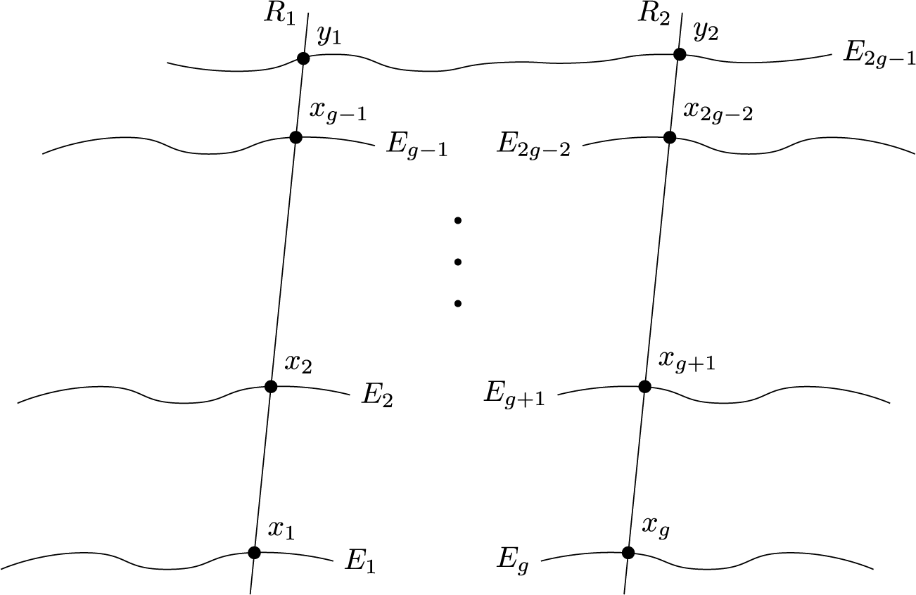


 Open access