

1 Introduction
1.1 Study motivation
In social and behavioral sciences, researchers use data collection strategies to represent the complexity of human behavior in real-world settings. A frequent design samples from multiple clusters, each reflecting a distinct subgroup of the target population (e.g., by demographic, geographic, or institutional characteristics). Many such datasets exhibit multilevel cross-classified structures in which individuals are simultaneously nested within more than one non-nested higher-level unit (e.g., Barker et al., Reference Barker, Dunn, Richmond, Ahmed, Hawrilenko and Evans2020; Goldstein, Reference Goldstein1994; Raudenbush & Bryk, Reference Raudenbush and Bryk2002). For example, students can be cross-classified by schools and neighborhoods, so that each student is associated with a specific school–neighborhood combination. In these settings, outcomes typically display statistical dependence arising from shared contextual or structural influences within clusters (e.g., school policies, teacher engagement, neighborhood socioeconomic conditions, and community norms). Accurately estimating effects of both individual-level and contextual-level variables therefore requires models that explicitly represent cross-classified clustering. Cross-classified multilevel models partition variance across multiple grouping factors, yielding more valid estimation and inferences and enhancing the generalizability of results obtained from observational, cross-sectional data (e.g., Raudenbush & Bryk, Reference Raudenbush and Bryk2002).
Arguably, the most widely used approach for modeling dependence is the linear mixed model (LMM; Laird & Ware, Reference Laird and Ware1982), which accounts for clustering-induced dependence through random effects. In the social and behavioral sciences, these models are also termed multilevel or hierarchical linear models. In many applications, a primary aim is to identify important predictors of an outcome across multiple social contexts (e.g., neighborhoods and schools; Harris & Halpern, Reference Harris and Halpern2022). LMMs accommodate both individual-level and cluster-level predictors to explain or predict variability in the outcome. Typical practice compares a set of candidate mixed-effects specifications that differ in the fixed-effect sets at each level, after which researchers interpret regression coefficients and test effects of substantive interest—procedures that remain standard in social and behavioral research.
Applying LMMs to investigate predictor–outcome relations presents challenges. First, functional form is often unknown: relations may be linear or nonlinear (e.g., logarithmic and exponential), and misspecification undermines model adequacy and interpretability. Second, predictors can interact in complex, non-additive ways, including higher-order interactions, which are difficult to specify a priori. Third, when the predictor set is large, identifying a parsimonious subset that meaningfully explains outcome variability is essential to avoid redundancy and overfitting while maintaining explanatory performance.
Machine-learning (ML) methods can capture complex, nonlinear associations between predictors and outcomes (e.g., Kuhn & Johnson, Reference Kuhn and Johnson2018). Among these, tree-ensemble approaches—random forests (RFs; Breiman, Reference Breiman2001) and gradient boosting (GB; Friedman, Reference Friedman2001)—aggregate many decision trees to improve predictive accuracy over a single tree (Breiman et al., Reference Breiman, Friedman, Olshen and Stone1984). By exploring diverse featureFootnote 1 subsets and splits, tree ensembles automatically accommodate nonlinearities and interactions. Moreover, RF and GB conduct implicit feature selection during training by preferentially splitting on informative variables, thereby elevating the influence of the most relevant predictors. Applications of RF and GB are increasingly common in the social and behavioral sciences (e.g., Jacobucci et al., Reference Jacobucci, Grimm and Zhang2023). A well-known limitation, however, is that standard ML implementations typically assume independent observations.
Taken together, current practice tends to rely on a limited set of prespecified effects within LMMs, with constrained support for systematic discovery of nonlinearities and interactions, limited scalability when many predictors are considered, and incomplete integration of data-adaptive diagnostics tailored to clustered designs. These limitations motivate complementary exploratory steps to enhance robustness and interpretability in exploratory analyses of multilevel data.
It is useful to clarify that the motivation for considering nonlinear and interaction effects in the present study is substantive. For example, in adolescent development, interactions (e.g., two level-1 predictors) and cross-level interactions are theoretically plausible and have been empirically documented, such as the moderating role of school connectedness in the association between bullying and aggressive or suicidal behaviors among sexual minority youth (e.g., Duong & Bradshaw, Reference Duong and Bradshaw2014).
1.2 Limitations of existing methods
Several modeling families address aspects of challenges of investigating predictor–outcome, yet each introduces practical tradeoffs. Parametric extensions (e.g., polynomial terms) require a priori choices about which predictors to model nonlinearly. Generalized additive mixed models (GAMMs; Hastie & Tibshirani, Reference Hastie and Tibshirani1986) and regularized LMMs provide flexible or shrinkage-based alternatives but still require decisions about smoothness, basis specification, and interaction structure, and their performance hinges on tuning choices. Nonparametric, data-adaptive ensembles (e.g., RF and GB), which are commonly treated as ML methods, can recover higher-order interactions and complex effect shapes without prespecifying functional forms; however, they likewise require principled complexity control and careful validation to mitigate overfitting. Within this nonparametric, data-adaptive class, interpretable ML methods can help to identify influential predictors, characterize predictor–outcome relationships (linear, monotonic, or complex), and probe interactions (e.g., Apley & Zhu, Reference Apley and Zhu2020; Friedman & Popescu, Reference Friedman and Popescu2008; Molnar, Reference Molnar2019) however, their use is not yet routine in exploratory workflows for multilevel data and often lacks cluster-aware implementation.
Because regular ML methods assume that all observations are independent, hybrid methods have been developed to incorporate ML techniques (e.g., tree-based or ensemble learning methods) into LMMs to account for dependencies due to clustering in multilevel data, as summarized in Table 1.Footnote 2 These hybrid methods leverage the strengths of ML while accounting for cluster-level dependencies in multilevel data. Simulation studies in prior work, as shown in Table 1, demonstrated that the hybrid models provided superior prediction accuracy compared to both standalone ML methods and LMMs. This prior work emphasized the importance of incorporating random effects to fully leverage the advantages of ML methods. However, as reviewed in Table 1, prior work has focused primarily on nested multilevel structures and has not addressed multilevel cross-classified structures. In addition, existing estimation methods are not directly applicable in this setting because prior work integrating ML with LMMs has primarily focused on tree-based or RF approaches under nested data structures (see Table 1). Furthermore, prior work has not demonstrated the interpretability of ML methods, such as importance measures, when they are used within hybrid approaches that combine ML techniques with LMMs.
Overview of literature reviews on LMM-ML for continuous outcomes

Note: RF indicates random forests; GB indicates gradient boosting; *Capitaine et al. (Reference Capitaine, Genuer and Thiébaut2021) used a variable selection procedure based on random forests, which is not typically categorized as an interpretable ML method in the sense of providing a formal variable importance measure.
Extreme gradient boosting (XGBoost; Chen & Guestrin, Reference Chen and Guestrin2016) is a scalable implementation of gradient-boosted decision trees that sequentially fits shallow trees to the negative gradients (pseudo-residuals) of a specified loss function. Compared to earlier boosting frameworks (e.g., Friedman, Reference Friedman2001), XGBoost introduces systematic
 $\ell _1/\ell _2$
regularization on leaf weights, shrinkage and column/row subsampling to reduce variance, and a second-order Taylor approximation for line search. These design features typically yield robustness to multicollinearity and complex interactions, and favorable bias–variance tradeoffs relative to single trees, RF, or unregularized boosting, while remaining compatible with smooth loss functions for continuous outcomes. To our knowledge, no prior hybrid method combines XGBoost with LMM for continuous responses—particularly not in multilevel cross-classified settings with crossed random effects—nor do prior studies develop estimation methods that preserve the random-effects structure while leveraging XGBoost’s regularized boosting and interaction modeling. Consequently, the interpretability layer specific to XGBoost (e.g., permutation importance aligned with clustered dependence) has also not been demonstrated within an LMM-ML hybrid framework.
$\ell _1/\ell _2$
regularization on leaf weights, shrinkage and column/row subsampling to reduce variance, and a second-order Taylor approximation for line search. These design features typically yield robustness to multicollinearity and complex interactions, and favorable bias–variance tradeoffs relative to single trees, RF, or unregularized boosting, while remaining compatible with smooth loss functions for continuous outcomes. To our knowledge, no prior hybrid method combines XGBoost with LMM for continuous responses—particularly not in multilevel cross-classified settings with crossed random effects—nor do prior studies develop estimation methods that preserve the random-effects structure while leveraging XGBoost’s regularized boosting and interaction modeling. Consequently, the interpretability layer specific to XGBoost (e.g., permutation importance aligned with clustered dependence) has also not been demonstrated within an LMM-ML hybrid framework.
ML methods, including XGBoost, are prone to memorize idiosyncratic patterns or noise in the training data. Cross-validation (CV) provides a principled way to quantify generalization error by evaluating model performance on held-out folds that were not used during training. Applying CV in multilevel cross-classified settings poses several challenges. Standard K-fold CV that randomly partitions individual observations breaks the multilevel structure, allowing units from the same cluster (e.g., school and neighborhood) to appear in both training and validation sets, which leads to information leakage and overly optimistic estimates of generalization error. In cross-classified designs, additional complications arise because each observation belongs to the cross of two or more higher-level units, making it nontrivial to define folds that simultaneously hold out entire combinations of clusters in a balanced way. Existing practice often relies on naïve observation-level CV or cluster-blocking on only one clustering factor (e.g., Roberts et al., Reference Roberts, Bahn, Ciuti, Boyce, Elith, Guillera-Arroita, Hauenstein, Lahoz-Monfort, Schröder, Thuiller, Warton, Wintle, Hartig and Dormann2017), both of which fail to fully respect the dependence structure and can misrepresent out-of-sample performance for new cross-classified structures (e.g., schools and neighborhoods). Moreover, widely used software defaults and tuning workflows rarely implement principled group- or combined-group CV for cross-classified multilevel data.
1.3 Study purposes and novel contributions
The purpose of this article is to develop a mixed-effects ML framework for modeling complex, nonlinear relationships between predictors and outcomes in multilevel, cross-classified data with continuous outcomes. The study makes four methodological contributions: (a) integrating XGBoost into the LMM (hereafter, LMM–XGBoost); (b) developing an estimation procedure for LMM–XGBoost; (c) developing a group-aware permutation importance measure; and (d) proposing combined-group CV for hyperparameter tuning, out-of-fold (OOF) prediction, and permutation importance. The accompanying R (R Core Team, 2025) functions, which fully automate these four components, is publicly available on the Open Science Framework (OSF), https://osf.io/jkctg/.
LMM–XGBoost is designed to capture nonlinear and interaction effects among predictors (a core strength of ML) while accommodating random effects due to clustering (a core feature of LMMs). As noted above, LMM–XGBoost outputs can be used in exploratory stages to enhance robustness and interpretability in subsequent analyses. LMM–XGBoost is illustrated with an empirical analysis investigating factors across multiple domains associated with adolescent depressive symptoms, with the aim of informing targeted mental-health interventions. In addition, simulation studies evaluate (a) the benefits of modeling nonlinear and interaction fixed effects in LMM–XGBoost relative to a standard LMM, (b) the advantages of incorporating crossed random effects in LMM–XGBoost relative to XGBoost alone, and (c) parameter recovery for LMM–XGBoost together with the accuracy of the proposed group-aware permutation importance.
The remainder of this article is organized as follows. In Section 2, LMM–XGBoost is specified, following presentations of LMM and XGBoost, respectively. In addition, the estimation method and conditional group-aware permutation importance measure are presented. In Section 3, the performance of the LMM–XGBoost relative to competing methods (LMM and XGBoost), the parameter recovery of LMM–XGBoost, and the accuracy of the conditional group-aware permutation importance measure are evaluated through simulation. In Section 4, LMM–XGBoost is applied using the Add Health data (Harris et al., Reference Harris, Halpern, Whitsel, Hussey, Killeya-Jones, Tabor and Dean2019), with comparisons to LMM and XGBoost. In Section 5, we conclude with a summary and a discussion.
2 Method
This section begins by specifying LMM for a cross-classified multilevel structure and XGBoost, respectively, followed by the hybrid model, LMM–XGBoost. Subsequently, the estimation method is described for LMM–XGBoost. In addition, the proposed group-aware permutation importance for LMM–XGBoost and combined-group CV methods are presented.
2.1 Model specification
2.1.1 LMM
LMM for a cross-classified multilevel structure (Goldstein, Reference Goldstein1994) is written as
 $$ \begin{align} y_{ijk} = \beta_0 + \mathbf{x}_{ijk}\boldsymbol{\beta} + u_{1j} + u_{2k} + \epsilon_{ijk}, \end{align} $$
where
 $y_{ijk}$
is the outcome for the i-th observation in cross-classified clusters j and k,
$y_{ijk}$
is the outcome for the i-th observation in cross-classified clusters j and k,
 $\beta _0$
is the fixed intercept,
$\beta _0$
is the fixed intercept,
 $\mathbf {x}_{ijk}$
is the matrix of predictors,
$\mathbf {x}_{ijk}$
is the matrix of predictors,
 $\boldsymbol {\beta }$
is the vector of fixed effects,
$\boldsymbol {\beta }$
is the vector of fixed effects,
 $u_{1j}$
is the random effect associated with cluster j,
$u_{1j}$
is the random effect associated with cluster j,
 $u_{2k}$
is the random effect associated with cluster k, and
$u_{2k}$
is the random effect associated with cluster k, and
 $\epsilon _{ijk}$
is the random residual. The
$\epsilon _{ijk}$
is the random residual. The
 $u_{1j}$
and
$u_{1j}$
and
 $u_{2k}$
are assumed to be additive and independent random effects;
$u_{2k}$
are assumed to be additive and independent random effects;
 $u_{1j} \sim \mathcal {N}(0,\sigma _{u1}^{2})$
and
$u_{1j} \sim \mathcal {N}(0,\sigma _{u1}^{2})$
and
 $u_{2k} \sim \mathcal {N}(0,\sigma _{u2}^{2})$
(Goldstein, Reference Goldstein1994). The
$u_{2k} \sim \mathcal {N}(0,\sigma _{u2}^{2})$
(Goldstein, Reference Goldstein1994). The
 $\epsilon _{ijk}$
is assumed to follow
$\epsilon _{ijk}$
is assumed to follow
 $\epsilon _{ijk} \sim \mathcal {N}(0, \sigma ^{2})$
.
$\epsilon _{ijk} \sim \mathcal {N}(0, \sigma ^{2})$
.
2.1.2 XGBoost
XGBoost (Chen & Guestrin, Reference Chen and Guestrin2016) is a highly optimized, distributed implementation of GB. It is used to approximate an unknown target function
 $f(\mathbf {x})$
that may involve complex nonlinearities and high-order interactions among predictors. Within the boosting framework formulated by Friedman (Reference Friedman2001), XGBoost constructs an additive ensemble of decision trees in a forward, stage-wise fashion. At boosting iteration m, a new tree
$f(\mathbf {x})$
that may involve complex nonlinearities and high-order interactions among predictors. Within the boosting framework formulated by Friedman (Reference Friedman2001), XGBoost constructs an additive ensemble of decision trees in a forward, stage-wise fashion. At boosting iteration m, a new tree
 $f_m(\mathbf {x})$
is appended to the current ensemble to further reduce residual error, so that after M iterations, the prediction is
$f_m(\mathbf {x})$
is appended to the current ensemble to further reduce residual error, so that after M iterations, the prediction is
 $$ \begin{align} \tilde{y}^{(M)} = \sum_{m=1}^{M} f_m(\mathbf{x}). \end{align} $$
The boosting iterations proceed until a convergence criterion is met or a prespecified stopping rule terminates the process.
XGBoost fits a single tree at each boosting iteration by optimizing a second-order Taylor expansion of the loss function with a structural regularization term. Specifically, at iteration m, the objective for the new tree
 $f_m(\mathbf {x}_n)$
, for observation n (
$f_m(\mathbf {x}_n)$
, for observation n (
 $n = 1, \ldots , N$
; n indexes observational units, each uniquely determined by the triplet
$n = 1, \ldots , N$
; n indexes observational units, each uniquely determined by the triplet
 $(i,j,k)$
), is
$(i,j,k)$
), is
 $$ \begin{align} \mathcal{L}^{(m)} = \sum_{n=1}^{N} \left[ g_n f_m(\mathbf{x}_n) + \frac{1}{2} h_{n} f_{m}^2(\mathbf{x}_n) \right] + \Omega(f_{m}), \end{align} $$
where
 $g_n$
and
$g_n$
and
 $h_n$
denote the first- and second-order derivatives of the loss with respect to the current prediction, respectively, and
$h_n$
denote the first- and second-order derivatives of the loss with respect to the current prediction, respectively, and
 $\Omega (f_m)$
controls the complexity of the newly added tree. The regularization term, which mitigates overfitting, is specified as
$\Omega (f_m)$
controls the complexity of the newly added tree. The regularization term, which mitigates overfitting, is specified as
 $$ \begin{align} \Omega(f_m) = \kappa V + \frac{1}{2}\lambda \sum_{v=1}^{V} ||\omega_v||^2, \end{align} $$
where v indexes terminal nodes (leaves), V is the number of leaves,
 $\omega _v$
is the prediction assigned to leaf v,
$\omega _v$
is the prediction assigned to leaf v,
 $\kappa $
penalizes tree size, and
$\kappa $
penalizes tree size, and
 $\lambda $
is an
$\lambda $
is an
 $\ell _2$
(ridge) penalty on the leaf values. Optionally, an additional
$\ell _2$
(ridge) penalty on the leaf values. Optionally, an additional
 $\ell _1$
(lasso) penalty,
$\ell _1$
(lasso) penalty,
 $\alpha \sum _{v=1}^{V} |\omega _v|$
, may be included, with
$\alpha \sum _{v=1}^{V} |\omega _v|$
, may be included, with
 $\alpha $
shrinking some leaf outputs exactly to zero and thereby inducing sparsity.
$\alpha $
shrinking some leaf outputs exactly to zero and thereby inducing sparsity.
To derive optimal leaf predictions and tree structure, the objective is simplified by aggregating gradient statistics at the leaf level. For a tree with V leaves, the per-tree objective (up to an additive constant) reduces to
 $$ \begin{align} \tilde{\mathcal{L}} = \sum_{v=1}^{V} \left[ G_v\omega_v + \frac{1}{2}(H_v+\lambda)\omega_v^{2} \right] + \kappa V, \end{align} $$
where
 $G_v$
and
$G_v$
and
 $H_v$
are the sums of the first- and second-order derivatives over all observations assigned to leaf v. This formulation leads to closed-form solutions for the optimal leaf weights and yields an efficient split-gain criterion for evaluating candidate partitions of the predictor space.
$H_v$
are the sums of the first- and second-order derivatives over all observations assigned to leaf v. This formulation leads to closed-form solutions for the optimal leaf weights and yields an efficient split-gain criterion for evaluating candidate partitions of the predictor space.
Key hyperparameters include the learning rate (eta), maximum depth of trees (max depth), minimum child weight (min child weight), regularization coefficients (lambda [
 $\ell _{2}\ \text {penalty}$
], alpha [
$\ell _{2}\ \text {penalty}$
], alpha [
 $\ell _{1}\ \text {penalty}$
]), minimum loss reduction required to create a split (gamma), subsampling fractions (subsample, colsample bytree), the number of boosting rounds (num boost round), and the number of early stopping rounds. For general introductions to tree-based boosting and the role of these hyperparameters, see Friedman (Reference Friedman2001), Hastie et al. (Reference Hastie, Tibshirani and Friedman2009, Chapters 9 and 10), and Chen and Guestrin (Reference Chen and Guestrin2016).
$\ell _{1}\ \text {penalty}$
]), minimum loss reduction required to create a split (gamma), subsampling fractions (subsample, colsample bytree), the number of boosting rounds (num boost round), and the number of early stopping rounds. For general introductions to tree-based boosting and the role of these hyperparameters, see Friedman (Reference Friedman2001), Hastie et al. (Reference Hastie, Tibshirani and Friedman2009, Chapters 9 and 10), and Chen and Guestrin (Reference Chen and Guestrin2016).
2.1.3 LMM–XGBoost
In LMM–XGBoost, the predicted values from XGBoost using an input
 $\mathbf {x}$
are incorporated into LMM, while allowing for random effects over cross-classified clusters. The LMM–XGBoost is presented as follows:
$\mathbf {x}$
are incorporated into LMM, while allowing for random effects over cross-classified clusters. The LMM–XGBoost is presented as follows:
 $$ \begin{align} y_{ijk} = \beta_0 + \mathrm{XG}(\mathbf{x}_{ijk}) + u_{1j} + u_{2k} + \epsilon_{ijk}, \end{align} $$
where
 $y_{ijk}$
is the outcome for the i-th observation in cross-classified clusters j and k,
$y_{ijk}$
is the outcome for the i-th observation in cross-classified clusters j and k,
 $\beta _{0}$
is the fixed intercept,
$\beta _{0}$
is the fixed intercept,
 $\mathrm {XG}(\mathbf {x}_{ijk})$
denotes the predicted value from XGBoost based on predictors
$\mathrm {XG}(\mathbf {x}_{ijk})$
denotes the predicted value from XGBoost based on predictors
 $\mathbf {x}_{ijk}$
,
$\mathbf {x}_{ijk}$
,
 $u_{1j}$
is the random effect associated with cluster j,
$u_{1j}$
is the random effect associated with cluster j,
 $u_{2k}$
is the random effect associated with cluster k, and
$u_{2k}$
is the random effect associated with cluster k, and
 $\epsilon _{ijk}$
is the random residual. The
$\epsilon _{ijk}$
is the random residual. The
 $u_{1j}$
and
$u_{1j}$
and
 $u_{2k}$
are assumed to be additive and independent random effects;
$u_{2k}$
are assumed to be additive and independent random effects;
 $u_{1j} \sim \mathcal {N}(0,\sigma _{u1}^{2})$
and
$u_{1j} \sim \mathcal {N}(0,\sigma _{u1}^{2})$
and
 $u_{2k} \sim \mathcal {N}(0,\sigma _{u2}^{2})$
(Goldstein, Reference Goldstein1994). The
$u_{2k} \sim \mathcal {N}(0,\sigma _{u2}^{2})$
(Goldstein, Reference Goldstein1994). The
 $\epsilon _{ijk}$
is assumed to follow
$\epsilon _{ijk}$
is assumed to follow
 $\epsilon _{ijk} \sim \mathcal {N}(0, \sigma ^{2})$
.
$\epsilon _{ijk} \sim \mathcal {N}(0, \sigma ^{2})$
.
In Equation (6), the crossed random effects
 $u_{1j}$
and
$u_{1j}$
and
 $u_{2k}$
are assumed to be uncorrelated with
$u_{2k}$
are assumed to be uncorrelated with
 $\mathbf {x}_{ijk}$
and to account fully for intracluster correlation, as in LMMs. Unlike conventional LMMs, however, parametric random slopes for predictor effects are not included. In LMMs, heterogeneity in predictor effects across clusters is typically modeled through random slopes, which represent unexplained cluster-specific deviations in the linear effects of predictors. In contrast, the LMM–XGBoost framework assumes that part of the apparent slope heterogeneity arises from systematic (non)linearities, interactions, or higher-order relationships among predictors. Such systematic heterogeneity can be flexibly captured by the XGBoost component, which learns complex predictor–outcome relationships without imposing a prespecified parametric form. Under this perspective, variability in predictor effects across clusters is partly explained through the ML component, while remaining unexplained cluster-level variation is captured through the random intercepts.
$\mathbf {x}_{ijk}$
and to account fully for intracluster correlation, as in LMMs. Unlike conventional LMMs, however, parametric random slopes for predictor effects are not included. In LMMs, heterogeneity in predictor effects across clusters is typically modeled through random slopes, which represent unexplained cluster-specific deviations in the linear effects of predictors. In contrast, the LMM–XGBoost framework assumes that part of the apparent slope heterogeneity arises from systematic (non)linearities, interactions, or higher-order relationships among predictors. Such systematic heterogeneity can be flexibly captured by the XGBoost component, which learns complex predictor–outcome relationships without imposing a prespecified parametric form. Under this perspective, variability in predictor effects across clusters is partly explained through the ML component, while remaining unexplained cluster-level variation is captured through the random intercepts.
Equation (6) cannot be estimated using a standard LMM estimation procedure because the fixed-effects component is replaced by a nonparametric function learned via XGBoost. Standard LMM estimation relies on a linear predictor with a finite set of parameters, whereas a boosted tree ensemble is an algorithmically estimated function whose structure is not parameterized within the LMM likelihood.
2.2 Estimation methods
This section first outlines two key components of the iterative LMM–XGBoost algorithm and then presents the full algorithm. The complete workflow is summarized in Algorithm 1.
2.2.1 Working residuals
The LMM in LMM–XGBoost assumes a Gaussian conditional distribution with an identity link. In this setting, the general iteratively reweighted least squares (IRLS)/Newton machinery collapses to a single weighted least-squares step for the conditional mean.
The fixed-effects component in LMM–XGBoost consists only of an intercept,
 $\boldsymbol {\beta } = (\beta _0)$
. Let n index an observation, uniquely identified by the triplet
$\boldsymbol {\beta } = (\beta _0)$
. Let n index an observation, uniquely identified by the triplet
 $(i,j,k)$
. For notational convenience, the multiple indices are replaced by the single observation index n. In the matrix formulation used for estimation, observations are stacked into a single response vector, and cluster membership is represented through the random-effect design matrices. The linear predictor of LMM–XGBoost is rewritten as
$(i,j,k)$
. For notational convenience, the multiple indices are replaced by the single observation index n. In the matrix formulation used for estimation, observations are stacked into a single response vector, and cluster membership is represented through the random-effect design matrices. The linear predictor of LMM–XGBoost is rewritten as
 $$ \begin{align} \eta_n \;=\; o_n \;+\; \beta_0 \;+\; \mathbf{z}_n^{\top}\mathbf{u}, \end{align} $$
where
 $o_n$
is a fixed, known offset
$o_n$
is a fixed, known offset
 $o_n = \text {XG}(\mathbf {x}_n)$
,
$o_n = \text {XG}(\mathbf {x}_n)$
,
 $\mathbf {u}$
is the vector of crossed random effects (
$\mathbf {u}$
is the vector of crossed random effects (
 ${\mathbf u}_{1}$
and
${\mathbf u}_{1}$
and
 ${\mathbf u}_{2}$
), and
${\mathbf u}_{2}$
), and
 $\mathbf {z}_n^{\top }$
is the row of the design matrix corresponding to observation n.
$\mathbf {z}_n^{\top }$
is the row of the design matrix corresponding to observation n.
The conditional log-likelihood for observation n is
 $$ \begin{align} \ell_n(\eta_n,\sigma^2) \;=\; -\tfrac{1}{2}\log(2\pi\sigma^2)\;-\;\frac{(y_n-\eta_n)^2}{2\sigma^2}. \end{align} $$
The score (
 $U_n$
) and the negative Hessian (
$U_n$
) and the negative Hessian (
 $H_n$
) with respect to the linear predictor
$H_n$
) with respect to the linear predictor
 $\eta _n$
are
$\eta _n$
are
 $$ \begin{align} U_n \;=\; \frac{\partial \ell_n}{\partial \eta_n} \;=\; \frac{y_n-\eta_n}{\sigma^2}, \qquad H_n \;=\; -\frac{\partial^2 \ell_n}{\partial \eta_n^2} \;=\; \frac{1}{\sigma^2}. \end{align} $$
A single Newton/IRLS step yields the working response and weight
 $$ \begin{align} e_n^{(t)} \;=\; \eta_n^{(t)} + \frac{U_n^{(t)}}{H_n^{(t)}} \;=\; \eta_n^{(t)} + \big(y_n-\eta_n^{(t)}\big) \;=\; y_n, \qquad \omega_n^{(t)} \;=\; H_n^{(t)} \;=\; \frac{1}{\sigma^2}. \end{align} $$
Thus, for the homoscedastic Gaussian model, the working response is simply the raw outcome (
 $\mathbf {e}=\mathbf {y}$
), and the precision weight is constant.
$\mathbf {e}=\mathbf {y}$
), and the precision weight is constant.
With the offset
 $\mathbf {o}=\text {XG}(\mathbf {x})$
, and the fixed-effect design matrix
$\mathbf {o}=\text {XG}(\mathbf {x})$
, and the fixed-effect design matrix
 $\mathbf {L}$
being a column vector of ones (corresponding to
$\mathbf {L}$
being a column vector of ones (corresponding to
 $\beta _0$
), the estimation proceeds by generalized least squares (GLS) on the shifted outcome:
$\beta _0$
), the estimation proceeds by generalized least squares (GLS) on the shifted outcome:
 $$ \begin{align} \mathbf{y}^{\ast} \;=\; \mathbf{y} \;-\; \mathbf{o}. \end{align} $$
The marginal covariance remains
 $$ \begin{align} \mathbf{V} \;=\; \mathbf{Z}\,\mathbf{G}\,\mathbf{Z}^{\top} \;+\; \sigma^2 \mathbf{I}, \end{align} $$
where
 $\mathbf G \;=\; \mathrm {blockdiag}\!\Big (\ \sigma _{u1}^2\,\mathbf I_{J}\ ,\ \sigma _{u2}^2\,\mathbf I_{K}\ \Big )$
. The Newton/GLS step for the fixed effects
$\mathbf G \;=\; \mathrm {blockdiag}\!\Big (\ \sigma _{u1}^2\,\mathbf I_{J}\ ,\ \sigma _{u2}^2\,\mathbf I_{K}\ \Big )$
. The Newton/GLS step for the fixed effects
 $\boldsymbol {\beta }$
solves the normal equations:
$\boldsymbol {\beta }$
solves the normal equations:
 $$ \begin{align} \big(\mathbf{L}^{\top}\mathbf{V}^{-1}\mathbf{L}\big)\,\Delta\boldsymbol{\beta} \;=\; \mathbf{L}^{\top}\mathbf{V}^{-1}\!\big(\mathbf{y}^{\ast} - \mathbf{Z}\widetilde{\mathbf{u}}\big), \end{align} $$
where
 $\widetilde {\mathbf {u}}$
are the conditional modes of the random effects.
$\widetilde {\mathbf {u}}$
are the conditional modes of the random effects.
The
 $\mathbf {y}^{\ast }$
term is modeled by
$\mathbf {y}^{\ast }$
term is modeled by
 $\mathbf {L}\boldsymbol {\beta } + \mathbf {Z}\widehat {\mathbf {u}}$
. Since
$\mathbf {L}\boldsymbol {\beta } + \mathbf {Z}\widehat {\mathbf {u}}$
. Since
 $\mathbf {L}\boldsymbol {\beta } = \beta _0\mathbf {1}$
(where
$\mathbf {L}\boldsymbol {\beta } = \beta _0\mathbf {1}$
(where
 $\mathbf {1}$
is a vector of ones), the working residual is
$\mathbf {1}$
is a vector of ones), the working residual is
 $$ \begin{align} \mathbf{r} \;=\; \mathbf{y}^{\ast} - \big(\mathbf{L}\boldsymbol{\beta} + \mathbf{Z}\widetilde{\mathbf{u}}\big) \;=\; \mathbf{y} \;-\; \mathbf{o} \;-\; \beta_0\mathbf{1} \;-\; \mathbf{Z}\widetilde{\mathbf{u}}. \end{align} $$
This setup corresponds to fitting a model where the fixed-effect component only includes the intercept
 $\beta _0$
. The offset
$\beta _0$
. The offset
 $\mathbf {o}$
captures the known predictions from XGBoost. The working residual
$\mathbf {o}$
captures the known predictions from XGBoost. The working residual
 $\mathbf {r}$
captures the variation remaining after subtracting the offset, the estimated intercept, and the predicted random effects.
$\mathbf {r}$
captures the variation remaining after subtracting the offset, the estimated intercept, and the predicted random effects.
2.2.2 The C-projection
The function
 $f(\mathbf {x})$
, learned by XGBoost on working residuals, can inadvertently absorb group-mean structure already accounted for by the cross-classified random effects (
$f(\mathbf {x})$
, learned by XGBoost on working residuals, can inadvertently absorb group-mean structure already accounted for by the cross-classified random effects (
 ${\mathbf u}_{1}$
and
${\mathbf u}_{1}$
and
 ${\mathbf u}_{2}$
). To enforce a clean separation between the random effects and the residual learner, we apply a weighted C-projection to the learner’s prediction vector, removing the span of the combined group dummies.
${\mathbf u}_{2}$
). To enforce a clean separation between the random effects and the residual learner, we apply a weighted C-projection to the learner’s prediction vector, removing the span of the combined group dummies.
In the LMM context with a Gaussian outcome, estimation is non-iterative and the IRLS precision weight is constant:
 $$ \begin{align} \omega_n \;=\; \frac{1}{\sigma^{2}} \quad \text{for all } n. \end{align} $$
Because this scalar factor is common to all terms in the projection, we may set the weight matrix proportional to the identity and, without loss of generality, take
 $\mathbf {W}=\mathbf {I}$
for the projection step.
$\mathbf {W}=\mathbf {I}$
for the projection step.
Let
 $\mathbf {Z}_{1}$
be the dummy (indicator) matrix for cluster j (random intercept
$\mathbf {Z}_{1}$
be the dummy (indicator) matrix for cluster j (random intercept
 $u_{1j}$
), and
$u_{1j}$
), and
 $\mathbf {Z}_2$
be the dummy matrix for cluster k (random intercept
$\mathbf {Z}_2$
be the dummy matrix for cluster k (random intercept
 $u_{2k}$
). Define the combined group-dummy matrix
$u_{2k}$
). Define the combined group-dummy matrix
 $$ \begin{align} \mathbf{Z} \;=\; \big[\,\mathbf{Z}_1 \;\; \mathbf{Z}_2\,\big]. \end{align} $$
Let
 $\mathbf {X}_g$
collect all group-constant predictors whose signal we intend to preserve (i.e., predictors constant within cluster j or within cluster k).
$\mathbf {X}_g$
collect all group-constant predictors whose signal we intend to preserve (i.e., predictors constant within cluster j or within cluster k).
Define the residual-maker that partials out
 $\mathbf {X}_g$
:
$\mathbf {X}_g$
:
 $$ \begin{align} \mathbf{M}_g \;=\; \mathbf{I} \;-\; \mathbf{X}_g \big(\mathbf{X}_g^\top \mathbf{X}_g\big)^{+} \mathbf{X}_g^\top, \qquad \tilde{\mathbf{Z}} \;=\; \mathbf{M}_g \mathbf{Z}, \end{align} $$
where
 $(\cdot )^{+}$
denotes the Moore–Penrose pseudoinverse.
$(\cdot )^{+}$
denotes the Moore–Penrose pseudoinverse.
Let
 $\tilde {\mathbf {f}}$
denote the raw XGBoost prediction vector (i.e.,
$\tilde {\mathbf {f}}$
denote the raw XGBoost prediction vector (i.e.,
 $\tilde {\mathbf {f}} = \mathrm {XG}(\mathbf {x})$
in (6)). The (weighted) C-projection in the Gaussian case reduces to the unweighted projection
$\tilde {\mathbf {f}} = \mathrm {XG}(\mathbf {x})$
in (6)). The (weighted) C-projection in the Gaussian case reduces to the unweighted projection
 $$ \begin{align} \tilde{\mathbf{f}}_{\perp} \;=\; \Big(\mathbf{I} - \tilde{\mathbf{Z}}\big(\tilde{\mathbf{Z}}^{\top}\tilde{\mathbf{Z}}\big)^{+}\tilde{\mathbf{Z}}^{\top}\Big)\,\tilde{\mathbf{f}}. \end{align} $$
This construction makes
 $f(\mathbf {x})$
orthogonal (in the Euclidean sense) to the combined group-dummy space spanned by the columns of
$f(\mathbf {x})$
orthogonal (in the Euclidean sense) to the combined group-dummy space spanned by the columns of
 $\mathbf {Z}$
while preserving the variation conveyed by the designated group-constant predictors
$\mathbf {Z}$
while preserving the variation conveyed by the designated group-constant predictors
 $\mathbf {X}_g$
. As a result, the LMM’s cross-classified structure is respected, and the effects of group-constant predictors are not inadvertently removed from the residual learner. A numerical illustration comparing no projection, naive Z-projection, and the proposed C-projection is provided in Appendix A.
$\mathbf {X}_g$
. As a result, the LMM’s cross-classified structure is respected, and the effects of group-constant predictors are not inadvertently removed from the residual learner. A numerical illustration comparing no projection, naive Z-projection, and the proposed C-projection is provided in Appendix A.
2.2.3 Algorithm
We implement an “E/M-style” alternating procedure in which a nonparametric learner updates the offset (E-step), and a mixed model updates the variance components and fixed intercept (M-step).
Initialization: Set
 $f^{(0)}(\mathbf x)\equiv 0$
,
$f^{(0)}(\mathbf x)\equiv 0$
,
 $\mathbf o^{(0)}=\mathbf 0$
. Fit an initial LMM with offset
$\mathbf o^{(0)}=\mathbf 0$
. Fit an initial LMM with offset
 $\mathbf o^{(0)}$
to obtain
$\mathbf o^{(0)}$
to obtain
 $\hat \beta _0^{(0)}$
,
$\hat \beta _0^{(0)}$
,
 $\widetilde {\mathbf u}^{(0)}$
, and variance components
$\widetilde {\mathbf u}^{(0)}$
, and variance components
 $\widehat {\boldsymbol \theta }^{(0)}=(\hat \sigma ^2,\hat \sigma _{u1}^2,\hat \sigma _{u2}^2)$
. Set
$\widehat {\boldsymbol \theta }^{(0)}=(\hat \sigma ^2,\hat \sigma _{u1}^2,\hat \sigma _{u2}^2)$
. Set
 $t=0$
.
$t=0$
.
E-step (nonparametric offset update): Form the working residual under the current fit
 $$\begin{align*}\mathbf r^{(t)} \;=\; \mathbf y \;-\; \mathbf o^{(t)} \;-\; \hat\beta_0^{(t)}\mathbf 1 \;-\; \mathbf Z\,\widetilde{\mathbf u}^{(t)}, \end{align*}$$
where the superscript
 $(t)$
indicates the current estimates at iteration t. Train XGBoost (Gaussian loss) on
$(t)$
indicates the current estimates at iteration t. Train XGBoost (Gaussian loss) on
 $\{(\mathbf x_n,\, r_n^{(t)})\}$
to obtain predictions
$\{(\mathbf x_n,\, r_n^{(t)})\}$
to obtain predictions
 $\tilde {\mathbf f}^{(t)}=\tilde f^{(t)}(\mathbf x)$
using the xgboost function in R implementation (Chen & Guestrin, Reference Chen and Guestrin2016; Chen et al., Reference Chen, He, Benesty, Khotilovich, Tang, Cho, Chen, Mitchell, Cano, Zhou, Li, Xie, Lin, Geng, Li and Yuan2025). In this function, the histogram-based tree construction algorithm is employed, which provides a scalable approximation to exact greedy split finding. We enforce orthogonality using the C-projection defined in Section 2.2.2
$\tilde {\mathbf f}^{(t)}=\tilde f^{(t)}(\mathbf x)$
using the xgboost function in R implementation (Chen & Guestrin, Reference Chen and Guestrin2016; Chen et al., Reference Chen, He, Benesty, Khotilovich, Tang, Cho, Chen, Mitchell, Cano, Zhou, Li, Xie, Lin, Geng, Li and Yuan2025). In this function, the histogram-based tree construction algorithm is employed, which provides a scalable approximation to exact greedy split finding. We enforce orthogonality using the C-projection defined in Section 2.2.2
Globally center the learner to keep the overall intercept in the fixed part:
 $$\begin{align*}\bar f^{(t)} \;=\; \frac{1}{N}\mathbf 1^\top \tilde{\mathbf f}_{\perp}^{(t)}, \qquad \mathbf f^{(t)} \;=\; \tilde{\mathbf f}_{\perp}^{(t)} - \bar f^{(t)}\mathbf 1. \end{align*}$$
M-step (mixed-model update): With
 $\mathbf y^\ast =\mathbf y-\mathbf o^{(t+1)}$
, refit the LMM to obtain
$\mathbf y^\ast =\mathbf y-\mathbf o^{(t+1)}$
, refit the LMM to obtain
 $\widehat {\beta }_{0}^{(t+1)}$
,
$\widehat {\beta }_{0}^{(t+1)}$
,
 $\widehat {\sigma }_{u1}^{2(t+1)}$
,
$\widehat {\sigma }_{u1}^{2(t+1)}$
,
 $\widehat {\sigma }_{u2}^{2(t+1)}$
, and
$\widehat {\sigma }_{u2}^{2(t+1)}$
, and
 $\widehat {\sigma }^{2(t+1)}$
. For the homoscedastic LMM, IRLS reduces to GLS on
$\widehat {\sigma }^{2(t+1)}$
. For the homoscedastic LMM, IRLS reduces to GLS on
 $\mathbf y^\ast $
with
$\mathbf y^\ast $
with
 $$\begin{align*}\big(\mathbf L^\top \mathbf V^{-1}\mathbf L\big)\,\Delta\boldsymbol\beta \;=\; \mathbf L^\top \mathbf V^{-1}\!\big(\mathbf y^\ast - \mathbf Z\,\widehat{\mathbf u}\big), \quad \mathbf L=\mathbf 1. \end{align*}$$
The M-step is implemented using the lmer function from the lme4 package (Bates et al., Reference Bates, Mächler, Bolker and Walker2015).
Learning rate
 $\alpha _{L}$
: At each iteration, the offset is updated by a convex combination of its previous value and the centered, C-projected learner increment:
$\alpha _{L}$
: At each iteration, the offset is updated by a convex combination of its previous value and the centered, C-projected learner increment:
 $$\begin{align*}\mathbf o^{(t+1)} \;=\; (1-\alpha_{L})\,\mathbf o^{(t)} \;+\; \alpha_{L}\,\mathbf f^{(t)}, \qquad \alpha_{L}\in(0,1]. \end{align*}$$
The parameter
 $\alpha _{L}$
acts as a step size controlling how aggressively the learner’s contribution is assimilated. When
$\alpha _{L}$
acts as a step size controlling how aggressively the learner’s contribution is assimilated. When
 $\alpha _{L}=1$
, the update fully incorporates the new increment (fast but potentially unstable); as
$\alpha _{L}=1$
, the update fully incorporates the new increment (fast but potentially unstable); as
 $\alpha _{L}\to 0$
, the update becomes more conservative, smoothing the sequence
$\alpha _{L}\to 0$
, the update becomes more conservative, smoothing the sequence
 $\{\mathbf o^{(t)}\}$
and reducing overfitting from any single iteration. Unfolding the recursion shows that
$\{\mathbf o^{(t)}\}$
and reducing overfitting from any single iteration. Unfolding the recursion shows that
 $\mathbf o^{(t)}$
is an exponentially weighted average of past increments,
$\mathbf o^{(t)}$
is an exponentially weighted average of past increments,
 $$\begin{align*}\mathbf o^{(t)} \;=\; (1-\alpha_{L})^t \mathbf o^{(0)} \;+\; \alpha_{L} \sum_{s=0}^{t-1} (1-\alpha_{L})^{t-1-s}\,\mathbf f^{(s)}, \end{align*}$$
so recent increments receive higher weight. Note that
 $\alpha _{L}$
scales only the assimilation of the fitted learner into the offset; it does not change the working residuals used to train the learner at iteration t. In practice,
$\alpha _{L}$
scales only the assimilation of the fitted learner into the offset; it does not change the working residuals used to train the learner at iteration t. In practice,
 $\alpha _{L}$
plays a role analogous to the shrinkage parameter in boosting and can be chosen alongside XGBoost’s own learning-rate and early-stopping settings.
$\alpha _{L}$
plays a role analogous to the shrinkage parameter in boosting and can be chosen alongside XGBoost’s own learning-rate and early-stopping settings.
A possible alternative approach would be to first remove cluster effects using a fixed-effects model and then apply XGBoost to the residualized outcome. However, this strategy differs from the proposed LMM–XGBoost framework in several important respects. First, residualizing the outcome using fixed effects removes cluster-level variation but does not estimate variance components associated with random effects or allow conditional predictions based on cluster-specific effects. Second, such preprocessing treats the clustering adjustment as a one-step procedure, whereas the proposed algorithm alternates between updating the ML component and estimating random effects. This iterative structure allows the nonlinear predictor learned by XGBoost and the random-effect estimates to be refined jointly during estimation. Third, the proposed framework naturally accommodates cross-classified clustering structures, whereas fixed-effects preprocessing would require introducing a large number of dummy variables and may become cumbersome in such settings. For these reasons, the proposed method provides a more integrated framework for combining ML with multilevel modeling than residualization followed by standalone XGBoost.
Convergence: A simpler rule such as checking the absolute or relative change in consecutive log-likelihoods of the fitted LMM,
 $\ell ^{(t)} - \ell ^{(t-1)}$
, against a tolerance
$\ell ^{(t)} - \ell ^{(t-1)}$
, against a tolerance
 $\varepsilon $
is often used but can be unreliable in the LMM–XGBoost algorithm. This method may halt prematurely after a transient small change due to noise in the XGBoost fit during the E-step or approximation error in the M-step’s variance component estimation, and it may fail to detect mild oscillations that indicate a lack of convergence. The iterative LMM–XGBoost algorithm employs a more robust method, checking for stability over a window of recent iterations, which is first applied after a user-configured starting iteration (e.g., the fourth iteration). The window size (e.g., the last few log-likelihood values) is a user-configurable parameter, as is the starting iteration for this check, to make the convergence criterion more robust to transient fluctuations. The algorithm terminates the iteration if the following condition holds:
$\varepsilon $
is often used but can be unreliable in the LMM–XGBoost algorithm. This method may halt prematurely after a transient small change due to noise in the XGBoost fit during the E-step or approximation error in the M-step’s variance component estimation, and it may fail to detect mild oscillations that indicate a lack of convergence. The iterative LMM–XGBoost algorithm employs a more robust method, checking for stability over a window of recent iterations, which is first applied after a user-configured starting iteration (e.g., the fourth iteration). The window size (e.g., the last few log-likelihood values) is a user-configurable parameter, as is the starting iteration for this check, to make the convergence criterion more robust to transient fluctuations. The algorithm terminates the iteration if the following condition holds:
 $t \ge 4$
and
$t \ge 4$
and
 $\operatorname {SD}\!\big (\ell ^{(t-4)},\ldots ,\ell ^{(t)}\big ) < \varepsilon $
, where
$\operatorname {SD}\!\big (\ell ^{(t-4)},\ldots ,\ell ^{(t)}\big ) < \varepsilon $
, where
 $\varepsilon $
is a user-specified tolerance (e.g., the standard deviation [SD] of the last three log-likelihoods). Otherwise, set
$\varepsilon $
is a user-specified tolerance (e.g., the standard deviation [SD] of the last three log-likelihoods). Otherwise, set
 $t \leftarrow t + 1$
and repeat.
$t \leftarrow t + 1$
and repeat.
2.3 Group-aware permutation importance for LMM–XGBoost
Permutation importance is defined as the loss inflation that occurs when the empirical link between one predictor and the fitted learner is destroyed while all other quantities are held fixed. Larger loss inflation implies a greater contribution of that predictor to predictive accuracy. Because the design is cross-classified, permutations respect grouping: (a) predictors that vary at the individual level are shuffled within each (Cluster1
 $\times $
Cluster2 id cell; i.e., permuted among rows sharing the same school and neighborhood) and (b) predictors that are constant within a cluster (e.g., school- or neighborhood-constant features, including elements of
$\times $
Cluster2 id cell; i.e., permuted among rows sharing the same school and neighborhood) and (b) predictors that are constant within a cluster (e.g., school- or neighborhood-constant features, including elements of
 $\mathbf {x}_{g}$
) are permuted at the corresponding cluster level and the permuted values are copied to all rows in that cluster. This procedure breaks the predictor–outcome association without fabricating cross-level combinations, thereby avoiding the bias of naïve global (row-wise) shuffling.
$\mathbf {x}_{g}$
) are permuted at the corresponding cluster level and the permuted values are copied to all rows in that cluster. This procedure breaks the predictor–outcome association without fabricating cross-level combinations, thereby avoiding the bias of naïve global (row-wise) shuffling.
The residual learner is trained on the working residuals (Equation (14)). Let
 $\tilde f(\mathbf x)$
denote the final centered and C-projected learner. Baseline predictions and loss on the evaluation data are
$\tilde f(\mathbf x)$
denote the final centered and C-projected learner. Baseline predictions and loss on the evaluation data are
 $$\begin{align*}\hat r_n^{(0)}=\tilde f(\mathbf x_n),\qquad M_0 = \mathrm{MSE}(\tilde f) = \frac{1}{N}\sum_{n=1}^N \big(r_n-\hat r_n^{(0)}\big)^2, \end{align*}$$
where MSE stands for mean squared error. During permutation, the fitted LMM–XGBoost (including C-projection and global centering applied to
 $\tilde f$
) is kept fixed; only the chosen predictor is permuted.
$\tilde f$
) is kept fixed; only the chosen predictor is permuted.
For predictor
 $x_q$
(where q indexes predictors), let
$x_q$
(where q indexes predictors), let
 $\pi _q$
be a group-aware permutation operator applied to
$\pi _q$
be a group-aware permutation operator applied to
 $x_q$
on the evaluation data. The permuted predictions and loss are
$x_q$
on the evaluation data. The permuted predictions and loss are
 $$\begin{align*}\hat r_n^{(\pi_q)}=\tilde f\!\big(\mathbf x_n^{\pi_q}\big), \qquad M_q=\frac{1}{N}\sum_{n=1}^N \big(r_n-\hat r_n^{(\pi_q)}\big)^2. \end{align*}$$
Importance is the average loss increase over D independent permutations:
 $$\begin{align*}\widehat{\Delta}_q=\frac{1}{D}\sum_{d=1}^D \big(M_{q,d}-M_0\big). \end{align*}$$

A nonnegative, normalized score is reported for readability:
 $$\begin{align*}\mathrm{RelImp}_q=\frac{\max(\widehat{\Delta}_q,0)}{\sum_j \max(\widehat{\Delta}_j,0)}. \end{align*}$$
Sampling variability across permutations is summarized by
 $$\begin{align*}\Delta_{q,\mathrm{sd}} =\sqrt{\frac{1}{D-1}\sum_{d=1}^D\Big[(M_{q,d}-M_0)-\widehat{\Delta}_q\Big]^2}. \end{align*}$$
In addition to full-sample permutation importance, generalization can be assessed with combined group K-fold CV. For each fold: (a) fit the full LMM–XGBoost pipeline on the training folds only (including tuning, iterative offset updates with learning rate
 $\alpha $
, C-projection, and global centering); (b) score the held-out fold to obtain
$\alpha $
, C-projection, and global centering); (b) score the held-out fold to obtain
 $M_0^{(\text {fold})}$
; and (c) apply group-aware permutations of
$M_0^{(\text {fold})}$
; and (c) apply group-aware permutations of
 $x_q$
within the held-out fold to compute
$x_q$
within the held-out fold to compute
 $M_{q,d}^{(\text {fold})}$
and
$M_{q,d}^{(\text {fold})}$
and
 $\Delta _{q,d}^{(\text {fold})}=M_{q,d}^{(\text {fold})}-M_0^{(\text {fold})}$
. The OOF importance aggregates across folds and permutations:
$\Delta _{q,d}^{(\text {fold})}=M_{q,d}^{(\text {fold})}-M_0^{(\text {fold})}$
. The OOF importance aggregates across folds and permutations:
 $$\begin{align*}\widehat{\Delta}_q^{\mathrm{OOF}}=\frac{1}{FR}\sum_{\text{fold}=1}^{F}\sum_{d=1}^{D}\Delta_{q,d}^{(\text{fold})}, \end{align*}$$
with the same truncation and normalization used for
 $\mathrm {RelImp}_q$
.
$\mathrm {RelImp}_q$
.
2.4 Combined group cross-validation
For tuning XGBoost in LMM–XGBoost, as well as for OOF prediction and permutation importance, the combined-group CV strategy was for cross-classified data structures, where observations are simultaneously nested within two higher-level clusters (e.g., schools and neighborhoods). Instead of grouping by only one clustering factor, this approach defines each unique pair of clusters—such as each specific school–neighborhood combination—as a distinct cross-classified cell and treats it as an indivisible unit during CV. All observations within the same cell are assigned to the same fold, ensuring that no cell contributes data to both the training and test sets. This blocking structure preserves dependencies arising from both clustering dimensions and prevents information leakage across either level.
3 Simulation study
In this section, simulation studies are presented to (a) evaluate the relative prediction accuracy of LMM–XGBoost, LMM, and XGBoost; (b) examine parameter recovery for LMM–XGBoost; and (c) assess the accuracy of group-aware permutation importance for LMM–XGBoost by comparing it with conventional permutation importance (naïve global shuffling) from XGBoost and LMM.
3.1 Simulation design and expected results
The varying simulation factors of variances of random effects and the number of clusters were designed to evaluate the relative performance of LMM–XGBoost versus LMM (linear effects only and no-interactions) and LMM–XGBoost versus XGBoost. Main and linear effects were considered for LMM because it serves as a baseline model for comparison. This choice does not imply that LMMs cannot handle interactions or nonlinearities; rather, it establishes a standard reference point to assess how data-driven methods, such as LMM–XGBoost, enhance explanatory performance over a traditionally specified LMM. Specifically, outcomes were generated with the following levels of the two varying simulation factors:
-
• Variances of random effects (ICCs): no, small, medium, and large.Footnote 3 For the no-variance level, the values of
 $\sigma _{u1}$
and
$\sigma _{u2}$
were both set to 0. While this scenario may be uncommon in practice, it was included to illustrate the maximal performance of XGBoost and the potential issue of boundary solutions (0 variances) in random effects for LMM and LMM–XGBoost. For the small variance level,
$\sigma _{u1}=\sigma _{u2}=0.130$
. For the chosen
$\sigma =0.551$
, this setting yields per-cluster ICCs
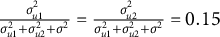
$\frac {\sigma _{u1}^{2}}{\sigma _{u1}^{2}+\sigma _{u2}^{2}+\sigma ^{2}}=\frac {\sigma _{u2}^{2}}{\sigma _{u1}^{2}+\sigma _{u2}^{2}+\sigma ^{2}}=0.05$
. For the medium variance level,
${\sigma _{u1}=\sigma _{u2}=0.255}$
, yielding per-cluster ICCs of
$0.15$
:
$\frac {\sigma _{u1}^{2}}{\sigma _{u1}^{2}+\sigma _{u2}^{2}+\sigma ^{2}}=\frac {\sigma _{u2}^{2}}{\sigma _{u1}^{2}+\sigma _{u2}^{2}+\sigma ^{2}}=0.15$
. For the large variance level,
$\sigma _{u1}=\sigma _{u2}=0.390$
, yielding per-cluster ICCs of
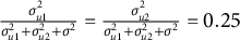
$0.25$
:
$\frac {\sigma _{u1}^{2}}{\sigma _{u1}^{2}+\sigma _{u2}^{2}+\sigma ^{2}}=\frac {\sigma _{u2}^{2}}{\sigma _{u1}^{2}+\sigma _{u2}^{2}+\sigma ^{2}}=0.25$
. These ICC magnitudes are consistent with values reported in applications of LMM or multilevel models (e.g., Snijders & Bosker, Reference Snijders and Bosker2012).
$\sigma _{u1}$
and
$\sigma _{u2}$
were both set to 0. While this scenario may be uncommon in practice, it was included to illustrate the maximal performance of XGBoost and the potential issue of boundary solutions (0 variances) in random effects for LMM and LMM–XGBoost. For the small variance level,
$\sigma _{u1}=\sigma _{u2}=0.130$
. For the chosen
$\sigma =0.551$
, this setting yields per-cluster ICCs
$\frac {\sigma _{u1}^{2}}{\sigma _{u1}^{2}+\sigma _{u2}^{2}+\sigma ^{2}}=\frac {\sigma _{u2}^{2}}{\sigma _{u1}^{2}+\sigma _{u2}^{2}+\sigma ^{2}}=0.05$
. For the medium variance level,
${\sigma _{u1}=\sigma _{u2}=0.255}$
, yielding per-cluster ICCs of
$0.15$
:
$\frac {\sigma _{u1}^{2}}{\sigma _{u1}^{2}+\sigma _{u2}^{2}+\sigma ^{2}}=\frac {\sigma _{u2}^{2}}{\sigma _{u1}^{2}+\sigma _{u2}^{2}+\sigma ^{2}}=0.15$
. For the large variance level,
$\sigma _{u1}=\sigma _{u2}=0.390$
, yielding per-cluster ICCs of
$0.25$
:
$\frac {\sigma _{u1}^{2}}{\sigma _{u1}^{2}+\sigma _{u2}^{2}+\sigma ^{2}}=\frac {\sigma _{u2}^{2}}{\sigma _{u1}^{2}+\sigma _{u2}^{2}+\sigma ^{2}}=0.25$
. These ICC magnitudes are consistent with values reported in applications of LMM or multilevel models (e.g., Snijders & Bosker, Reference Snijders and Bosker2012). -
• The number of clusters: small versus large.
The simulation study conditions for the number of clusters (J and K) and observations per cell (
$I_{jk}$
) were selected based on established multilevel literature. The number of clusters for both factors was set at two values,
$J=K=50$
and
$J=K=100$
. The former represents the minimum acceptable clusters often cited to mitigate bias in variance-component estimates (
$\sigma _{u1}^{2}$
and
$\sigma _{u2}^{2}$
) (Maas & Hox, Reference Maas and Hox2004), whereas the latter serves as a benchmark for maximizing estimator stability and accuracy (Clarke & Wheaton, Reference Clarke and Wheaton2007). The number of observations per cell,
$I_{jk}$
, was fixed at a constant, moderate value of
$5$
. This choice ensures an adequate Level-1 sample size to estimate the Level-1 residual variance (
$\sigma ^{2}$
) across all cluster combinations and satisfies the identification requirement
$I_{jk}>1$
.


The data-generating model is an LMM-tree (one “true” tree) under two varying simulation conditions. At Level-1, 10 continuous predictors were sampled from a multivariate normal distribution
 $\mathcal {MVN}(\mathbf {0},\Sigma _{L1})$
, where
$\mathcal {MVN}(\mathbf {0},\Sigma _{L1})$
, where
 $\Sigma _{L1}$
had unit variances and off-diagonal correlations of
$\Sigma _{L1}$
had unit variances and off-diagonal correlations of
 $0.2$
. A Cholesky decomposition of the correlation matrix was used to ensure positive definiteness. In addition, two Level-1 categorical predictors were generated via multinomial draws: one with two levels
$0.2$
. A Cholesky decomposition of the correlation matrix was used to ensure positive definiteness. In addition, two Level-1 categorical predictors were generated via multinomial draws: one with two levels
 $(0.5,0.5)$
and one with three levels
$(0.5,0.5)$
and one with three levels
 $(0.2,0.5,,0.3)$
. For the Cluster1-level predictors, three continuous variables were sampled from
$(0.2,0.5,,0.3)$
. For the Cluster1-level predictors, three continuous variables were sampled from
 $\mathcal {MVN}(\mathbf {0},\Sigma _{C1})$
with unit variances and pairwise correlations of
$\mathcal {MVN}(\mathbf {0},\Sigma _{C1})$
with unit variances and pairwise correlations of
 $0.2$
, and one categorical predictor with two levels
$0.2$
, and one categorical predictor with two levels
 $(0.5,,0.5)$
was generated via a multinomial draw. For the Cluster2-level predictors, three continuous variables were sampled from
$(0.5,,0.5)$
was generated via a multinomial draw. For the Cluster2-level predictors, three continuous variables were sampled from
 $\mathcal {MVN}(\mathbf {0},\Sigma _{C2})$
with unit variances and pairwise correlations of
$\mathcal {MVN}(\mathbf {0},\Sigma _{C2})$
with unit variances and pairwise correlations of
 $0.2$
, and one categorical predictor with three levels
$0.2$
, and one categorical predictor with three levels
 $(0.2,0.5,,0.3)$
was generated analogously. Cluster-level predictors were realized once per cluster and were identical for all observations sharing the corresponding cluster identifier (i.e., invariant within Cluster1 or Cluster2). The true tree was generated using 30 randomly selected variables drawn from the 20 continuous predictors and 37
$(0.2,0.5,,0.3)$
was generated analogously. Cluster-level predictors were realized once per cluster and were identical for all observations sharing the corresponding cluster identifier (i.e., invariant within Cluster1 or Cluster2). The true tree was generated using 30 randomly selected variables drawn from the 20 continuous predictors and 37
 $(=49-12)$
dummy predictors (from 12 generated categorical predictors, except the first level of each categorical predictor) predictors were considered. The decision tree was defined as a deterministic function of the 30 selected predictors, using fixed cutpoints held constant simulation across conditions. The true tree structure is shown in Appendix B.
$(=49-12)$
dummy predictors (from 12 generated categorical predictors, except the first level of each categorical predictor) predictors were considered. The decision tree was defined as a deterministic function of the 30 selected predictors, using fixed cutpoints held constant simulation across conditions. The true tree structure is shown in Appendix B.
The total number of simulation conditions is 8, comprising four levels of variances of random effects and two levels of the number of clusters. For each simulation condition, 1,000 replications were conducted. The LLM with linear and main effects, XGBoost, and LLM–XGBoost models were fitted to the same generated data sets. That is, the total number of simulation runs is 24,000 (
 $=$
8 conditions
$=$
8 conditions
 $\times $
1,000 replications
$\times $
1,000 replications
 $\times $
3 models).
$\times $
3 models).
In generating outcomes for each simulation condition, the true tree and the generated predictors were set to the same across the replications, and the random effects were generated at each replication in the simulation condition. The same cluster identifiers for the two cross-classified clusters (e.g., schools and neighborhoods) were used across replications. In data generation,
 $\beta _{0}=0$
was specified, and standardized predicted values from the true tree structure were used to estimate
$\beta _{0}=0$
was specified, and standardized predicted values from the true tree structure were used to estimate
 $\beta _{0}$
.
$\beta _{0}$
.
Evaluation measures were: (a) mean squared error (MSE) for relative model accuracy; (b) bias and root MSE (RMSE) for parameter recovery; and (c) Spearman’s rank correlation between true and estimated permutation importance to evaluate the accuracy of group-aware permutation importance. For the MSE of LMM and LMM–XGBoost, four variants were considered for comparison: (a) full-sample conditional MSE (with random-effect predictions), (b) full-sample marginal MSE (without random-effect predictions), (c) OOF conditional MSE, and (d) OOF marginal MSE. Conditional versus marginal MSE distinguishes model performance attributable to cluster-specific random effects from that explained by the fixed-effects component alone. Conditional predictions correspond to predicting new observations within clusters observed in the training data, whereas marginal predictions correspond to predicting outcomes for new clusters where cluster-specific random effects are unavailable. Full-sample MSE quantifies how well the fitted model matches the estimation data, whereas OOF MSE assesses generalization to held-out clusters or units, thereby reducing overfitting bias. The true permutation importance was computed from the true tree structure using the group-aware procedure described in Section 2.4. Group-aware permutation importance was estimated for LMM–XGBoost. Conventional (row-shuffling) permutation importance was computed for XGBoost and for LMM, reflecting common practice (e.g., Breiman, Reference Breiman2001; Fisher et al., Reference Fisher, Rudin and Dominici2019). For LMM, permutation scores were calculated using predictions from the fixed-effects component only. Because the true tree selects predictors from both Level-1 and cluster-level variables, the rank correlation between the true and estimated permutation importance implicitly evaluates the recovery of importance across predictors operating at different hierarchical levels. Permutation importance was evaluated both full-sample (to characterize the behavior of the fitted models with minimal resampling variance) and under CV (to assess generalizability).
For the selected simulation levels of the two varying conditions, the following patterns are expected. First, the LMM–XGBoost model yields the smallest conditional MSE when the random-effect variances are non-zero because the predictions condition on the estimated random effects, leaving primarily residual variation unexplained. The marginal MSE from LMM–XGBoost is larger because the marginal predictions average over the random effects and therefore do not include the realized cluster-specific deviations present in the observed outcomes. In contrast, the XGBoost model is trained directly on the observed responses and may partially capture between-cluster structure through predictors whose distributions vary across clusters. Consequently, its MSE is expected to lie between the conditional and marginal MSEs from LMM–XGBoost. Second, the marginal MSE from LMM and LMM–XGBoost is expected to increase as the ICC increases because the marginal predictions do not account for cluster-specific random effects. Third, for parameter recovery, the bias and RMSE of the fixed intercept are expected to increase as ICC increases and the number of clusters decreases, because the empirical mean of the random effects deviates more from zero when between-cluster variability is larger and fewer clusters are available to average out this variability. The random-effects SDs are expected to show decreasing bias as ICC and the number of clusters increase, whereas their RMSE increases with ICC (because they are estimated on a larger absolute scale) and decreases with the number of clusters. For the residual SD, both bias and RMSE are expected to show little dependence on ICC and to decrease as the number of clusters increases. Fourth, group-aware permutation importance from LMM–XGBoost is expected to outperform conventional (row-shuffling) permutation importance from XGBoost and LMM because it preserves the clustered (and cross-classified) dependence structure during permutation. At the no-variance level, the accuracy of the permutation importance measure is expected to be similar between LMM–XGBoost and XGBoost. In the presence of ICCs (i.e., non-zero variances), the accuracy of permutation importance under LMM–XGBoost is expected to exceed that of XGBoost, with the performance gap widening as ICC increases.
3.2 Analyses
In the residual-learning stage of XGBoost and the XGBoost component of the LMM–XGBoost, hyperparameters were selected using a grid search to balance capacity and stability under the simulation design. The learning rate (eta) was tuned as
 $\in {0.02, 0.03, 0.05}$
for trees with depth
$\in {0.02, 0.03, 0.05}$
for trees with depth
 $d \le 5$
and restricted to
$d \le 5$
and restricted to
 ${0.02, 0.03}$
for deeper trees (
${0.02, 0.03}$
for deeper trees (
 $d=6$
). The maximum tree depth (max depth) was set to
$d=6$
). The maximum tree depth (max depth) was set to
 $d \in {3, 4, 5}$
for
$d \in {3, 4, 5}$
for
 $N \approx 1.25 \times 10^{4}$
and
$N \approx 1.25 \times 10^{4}$
and
 $d \in {3, 4, 5, 6}$
for
$d \in {3, 4, 5, 6}$
for
 $N \approx 5.0 \times 10^{4}$
, constraining interaction order. The expected observations per terminal node were approximately
$N \approx 5.0 \times 10^{4}$
, constraining interaction order. The expected observations per terminal node were approximately
 $N / 2^{d}$
, yielding
$N / 2^{d}$
, yielding
 $\approx 1.6 \times 10^{3}$
,
$\approx 1.6 \times 10^{3}$
,
 $7.8 \times 10^{2}$
, and
$7.8 \times 10^{2}$
, and
 $3.9 \times 10^{2}$
for
$3.9 \times 10^{2}$
for
 $d=3,4,5$
when
$d=3,4,5$
when
 $N=1.25\times 10^{4}$
, and
$N=1.25\times 10^{4}$
, and
 $\approx 6.3 \times 10^{3}$
,
$\approx 6.3 \times 10^{3}$
,
 $3.1 \times 10^{3}$
,
$3.1 \times 10^{3}$
,
 $1.6 \times 10^{3}$
, and
$1.6 \times 10^{3}$
, and
 $7.8 \times 10^{2}$
for
$7.8 \times 10^{2}$
for
 $d=3,4,5,6$
when
$d=3,4,5,6$
when
 $N=5.0\times 10^{4}$
. Because unit sample weights were used, the leaf curvature H equals the number of training cases in each leaf under the squared-error objective (reg:squarederror); thus, the minimum child weight (min child weight) sets a lower bound on the minimum leaf size. The grid was adjusted by ICC level:
$N=5.0\times 10^{4}$
. Because unit sample weights were used, the leaf curvature H equals the number of training cases in each leaf under the squared-error objective (reg:squarederror); thus, the minimum child weight (min child weight) sets a lower bound on the minimum leaf size. The grid was adjusted by ICC level:
 $\texttt {min child weight} \in {25, 50, 75}$
for none or small ICCs (0.00–0.05),
$\texttt {min child weight} \in {25, 50, 75}$
for none or small ICCs (0.00–0.05),
 ${50, 100}$
for medium ICC
${50, 100}$
for medium ICC
 $(0.15)$
, and
$(0.15)$
, and
 ${75, 150}$
for large ICC
${75, 150}$
for large ICC
 $(0.25)$
; for
$(0.25)$
; for
 $d=6$
(available only when
$d=6$
(available only when
 $N = 5.0 \times 10^{4}$
), an additional value
$N = 5.0 \times 10^{4}$
), an additional value
 $200$
was included.
$200$
was included.
 $\ell _{2}$
regularization (lambda) explored
$\ell _{2}$
regularization (lambda) explored
 $\lambda \in {1, 3, 10, 30}$
to shrink leaf values and stabilize small partitions. For the
$\lambda \in {1, 3, 10, 30}$
to shrink leaf values and stabilize small partitions. For the
 $\ell _{1}$
penalty, alpha was set to
$\ell _{1}$
penalty, alpha was set to
 ${0, 0.5, 1, 3}$
. Under XGBoost’s second-order objective, the optimal leaf value is defined as
${0, 0.5, 1, 3}$
. Under XGBoost’s second-order objective, the optimal leaf value is defined as
 $\omega ^{*} \;=\; -\,(H + \lambda )^{-1} \, \operatorname {sgn}(G)\, \max \!\big (|G| - \alpha ,\,0\big )$
(Chen & Guestrin, Reference Chen and Guestrin2016), where
$\omega ^{*} \;=\; -\,(H + \lambda )^{-1} \, \operatorname {sgn}(G)\, \max \!\big (|G| - \alpha ,\,0\big )$
(Chen & Guestrin, Reference Chen and Guestrin2016), where
 $\texttt {alpha}=\alpha $
applies soft-thresholding to the summed gradient G, and
$\texttt {alpha}=\alpha $
applies soft-thresholding to the summed gradient G, and
 $\texttt {lambda}=\lambda $
inflates curvature H (ridge shrinkage). On this scale,
$\texttt {lambda}=\lambda $
inflates curvature H (ridge shrinkage). On this scale,
 $\alpha \in [0.5, 3]$
induces mild-to-moderate sparsity, zeroing leaves whose signal is near noise while preserving substantive effects; this complements the smoother
$\alpha \in [0.5, 3]$
induces mild-to-moderate sparsity, zeroing leaves whose signal is near noise while preserving substantive effects; this complements the smoother
 $\ell _{2}$
shrinkage from
$\ell _{2}$
shrinkage from
 $\lambda \in {1, 3, 10, 30}$
. Including
$\lambda \in {1, 3, 10, 30}$
. Including
 $\alpha = 0$
ensures a baseline without
$\alpha = 0$
ensures a baseline without
 $\ell _{1}$
regularization,
$\ell _{1}$
regularization,
 $\alpha = 0.5$
–1 provides light sparsity to reduce variance when residual signal is diffuse across predictors, and
$\alpha = 0.5$
–1 provides light sparsity to reduce variance when residual signal is diffuse across predictors, and
 $\alpha = 3$
offers stronger regularization for sensitivity analyses or deeper trees with many small leaves. Larger
$\alpha = 3$
offers stronger regularization for sensitivity analyses or deeper trees with many small leaves. Larger
 $\alpha $
values were avoided to prevent over-sparsification given moderate H. The search permitted up to num boost round
$\alpha $
values were avoided to prevent over-sparsification given moderate H. The search permitted up to num boost round
 $=1{,}200$
with early stopping and used RMSE as the tuning criterion. Hyperparameter selection employed a combined five-fold CV, with subsampling ratios fixed at colsample bytree
$=1{,}200$
with early stopping and used RMSE as the tuning criterion. Hyperparameter selection employed a combined five-fold CV, with subsampling ratios fixed at colsample bytree
 $=1.0$
and subsample
$=1.0$
and subsample
 $=1.0$
to prevent cross-cluster leakage.
$=1.0$
to prevent cross-cluster leakage.
In LMM–XGBoost, the tuning constants were set to
 $\epsilon =0.4$
and
$\epsilon =0.4$
and
 $\alpha _{L}=0.5$
. Empirically, with
$\alpha _{L}=0.5$
. Empirically, with
 $\epsilon =0.4$
, the estimates in LMM–XGBoost (
$\epsilon =0.4$
, the estimates in LMM–XGBoost (
 $\widehat {\beta }_{0}$
,
$\widehat {\beta }_{0}$
,
 $\widehat {\beta }_{1}$
,
$\widehat {\beta }_{1}$
,
 $\widehat {\sigma }_{u1}^{2}$
,
$\widehat {\sigma }_{u1}^{2}$
,
 $\widehat {\sigma }_{u2}^{2}$
,
$\widehat {\sigma }_{u2}^{2}$
,
 $\widehat {\sigma }$
) differed only in the fourth or fifth decimal place between successive iterations. For permutation-based importance, 1,000 permutations were used for both the group-aware permutation importance from LMM–XGBoost and the conventional (global shuffle, unconditional) permutation importance from XGBoost. For comparison purposes, both the full-sample and the OOF importance estimates were obtained. LMM–XGBoost exhibited no convergence problems in any condition. The number of iterations required for convergence ranged from 10 to 45 across 8,000 runs (8 conditions
$\widehat {\sigma }$
) differed only in the fourth or fifth decimal place between successive iterations. For permutation-based importance, 1,000 permutations were used for both the group-aware permutation importance from LMM–XGBoost and the conventional (global shuffle, unconditional) permutation importance from XGBoost. For comparison purposes, both the full-sample and the OOF importance estimates were obtained. LMM–XGBoost exhibited no convergence problems in any condition. The number of iterations required for convergence ranged from 10 to 45 across 8,000 runs (8 conditions
 $\times $
1,000 replications).
$\times $
1,000 replications).
3.3 Results
Table 2 reports the simulation results averaged over 1,000 replications for the full sample and the OOF values. Overall, the expected patterns were observed, with a few exceptions. Monte Carlo standard errors were computed to assess simulation uncertainty. With 1,000 replications, the resulting Monte Carlo standard errors were typically below 0.01 for the reported summaries and therefore negligible relative to the differences observed across methods.
Simulation results: Panel A (prediction accuracy), Panel B (parameter recovery), and Panel C (accuracy of permutation importance)

Table 2, Panel A, presents the MSE under LMM, XGBoost, and LMM–XGBoost for the full sample and OOF. Across both the full sample and OOF, the MSE from LMM was the largest, indicating that ignoring interactions and nonlinearity in LMM led to poorer predictive performance. In addition, the marginal MSEs from LMM and LMM–XGBoost increased as the ICC increased in both the full sample and OOF. With OOF, the conditional MSE from LMM–XGBoost was the smallest, and, as expected, it fell between the conditional and marginal MSEs from LMM–XGBoost when the random-effect variances were non-zero. However, with the full sample, the MSE from XGBoost was smaller than or equal to the conditional MSE from LMM–XGBoost under non-zero random-effect variances. This may be due to the downward bias of full-sample MSE for XGBoost, which can partially absorb random-effect variation and overfit idiosyncratic patterns when predictions are evaluated on the same data used for training.
Table 2, Panel B, shows bias and RMSE of parameter estimates from LMM–XGBoost. Across all simulation conditions, the fixed intercept exhibited increasing bias in absolute value and larger RMSE as the variance of the random effects (or ICC) increased, with both bias and RMSE reduced when the number of clusters was larger. For the random-effects SDs (
 $\sigma _{u1}$
and
$\sigma _{u1}$
and
 $\sigma _{u2}$
), bias decreased as the random-effect variance (or ICC) increased and as the number of clusters increased, indicating improved centering of these estimators when between-cluster variability was stronger and more clusters were available. Their RMSE, however, increased with larger random-effect variance (reflecting greater absolute estimation error on a larger scale) and decreased with more clusters. In contrast, the residual SD (
$\sigma _{u2}$
), bias decreased as the random-effect variance (or ICC) increased and as the number of clusters increased, indicating improved centering of these estimators when between-cluster variability was stronger and more clusters were available. Their RMSE, however, increased with larger random-effect variance (reflecting greater absolute estimation error on a larger scale) and decreased with more clusters. In contrast, the residual SD (
 $\sigma $
) showed relatively stable bias and RMSE across different levels of random-effect variance, with both measures modestly smaller when more clusters were available. Under the zero-variance conditions, LMM–XGBoost tended to overestimate the random-effect SD and exhibited larger sampling variability, rather than showing convergence issues due to boundary solutions.
$\sigma $
) showed relatively stable bias and RMSE across different levels of random-effect variance, with both measures modestly smaller when more clusters were available. Under the zero-variance conditions, LMM–XGBoost tended to overestimate the random-effect SD and exhibited larger sampling variability, rather than showing convergence issues due to boundary solutions.
Table 2, Panel C, reports the rank correlations between the true importance measures and the estimated permutation importance from LMM, XGBoost, and LMM–XGBoost for the full sample and OOF. Across all conditions and methods, the full-sample and OOF importance estimates were comparable. Across all conditions, LMM–XGBoost yielded the highest rank correlations, which were uniformly high, ranging from 0.976 to 0.995. When the random-effect variances were zero, the accuracy of LMM–XGBoost and XGBoost was similar, particularly in the large-sample OOF condition where their rank correlations were identical, although LMM–XGBoost still outperformed XGBoost in the small-sample conditions. In the presence of non-zero variances, the rank correlations for XGBoost and LMM deteriorated as ICC increased, whereas those for LMM–XGBoost remained high, so that the performance gap between LMM–XGBoost and XGBoost widened with increasing ICC.
4 Applications
In this section, the method described in Section 2 is applied to the Add Health data to take an advantage of rich data on depressive symptoms. The objective of the analysis is to comprehensively investigate the multi-domain factors of adolescent depressive symptoms, aiming to inform more effective and targeted mental health interventions.
4.1 Samples
Add Health is a nationally representative sample from the United States, comprising over 20,000 adolescents in grades 7–12 during the 1994–1995 school year (Harris et al., Reference Harris, Halpern, Whitsel, Hussey, Killeya-Jones, Tabor and Dean2019). These participants have been tracked for 25 years, spanning into early midlife, through five waves of interviews. In this study, Wave 1 data (interviewed 1994–1995;
 $N=20,745$
) were selected. Add Health restricted-use data contract and Institutional Review Board approval were obtained.
$N=20,745$
) were selected. Add Health restricted-use data contract and Institutional Review Board approval were obtained.
Add Health data used 132-school representative of youth in the United States (52 middle schools and 80 high schools; PSUSCID variable) (Harris, Reference Harris2013). Cases with missing sampling weights were deleted. After deletion, the total number of participants was 18,924. There were 2,344 neighborhood identifiers defined as the 1990 U.S. census tracts (W1NHOOD1 variable), and 170 missing cases of neighborhood identifiers. Thus, 18,754 participants (18,924
 $-$
170 missing cases of neighborhood identifiers) who were cross-classified by 132 schools and 2,344 neighborhoods were considered for analyses.
$-$
170 missing cases of neighborhood identifiers) who were cross-classified by 132 schools and 2,344 neighborhoods were considered for analyses.
4.2 Outcomes and predictors
4.2.1 Outcomes
Depressive symptoms at Wave 1 were assessed using a modified version of the Center for Epidemiologic Studies Depression Scale (CES-D) (Perreira et al., Reference Perreira, Deeb-Sossa, Harris and Bollen2005; Radloff, Reference Radloff1977). The modified 19-item version used in this study demonstrated good reliability in prior work (Perreira et al., Reference Perreira, Deeb-Sossa, Harris and Bollen2005). Responses were recorded as 0 (“never or rarely”), 1 (“sometimes”), 2 (“a lot of the time”), and 3 (“most or all of the time or all of the time”). In this article, the sum scores of 19 items (H1FS1 through H1FS19 from the Wave I in-home interview) were used, with items H1FS4, H1FS8, H1FS11, and H1FS15 reverse-coded, and responses of “refuse” (response of 6), “don’t know” (response of 8), and “not applicable” (response of 9) treated as missing data. Higher sum scores represent greater depressive symptoms. The distribution of the sum scores exhibited moderate right skewness and lighter tails (skewness
 $=1.08$
, kurtosis
$=1.08$
, kurtosis
 $=1.57$
). Therefore, the sum scores were square-root transformed to approximate normality, as was done with CES-D data in previous work with the Add Health dataset (e.g., Dawson et al., Reference Dawson, Wu, Fennie, Ibañez, Cano, Pettit and Trepka2019). After the square-root transformation, only two observations (participants) were identified as extreme points that deviated significantly from the normal distribution. However, because the deviation was small, the two observations were retained for analyses.
$=1.57$
). Therefore, the sum scores were square-root transformed to approximate normality, as was done with CES-D data in previous work with the Add Health dataset (e.g., Dawson et al., Reference Dawson, Wu, Fennie, Ibañez, Cano, Pettit and Trepka2019). After the square-root transformation, only two observations (participants) were identified as extreme points that deviated significantly from the normal distribution. However, because the deviation was small, the two observations were retained for analyses.
For 18,754 participants cross-classified by 132 schools and 2,344 neighborhoods, the median number of students per school is 123 (range
 $=[1, 1703]$
; SIQR
$=[1, 1703]$
; SIQR
 $=43$
), and the median number of students per neighborhood is 2 (range
$=43$
), and the median number of students per neighborhood is 2 (range
 $=[1, 275]$
; SIQR
$=[1, 275]$
; SIQR
 $=2$
). Each neighborhood includes one or multiple schools, ranging from 1 to 3. In addition, each school draws students from one or multiple neighborhoods, ranging from 1 to 224. Based on the unconditional LMM, the intraclass correlation (ICC) for schools and neighborhoods was calculated as 0.043, indicating that 4.3% of the total variance in students’ depressive symptoms is attributable to differences between the schools they attended and neighborhoods they lived in.
$=2$
). Each neighborhood includes one or multiple schools, ranging from 1 to 3. In addition, each school draws students from one or multiple neighborhoods, ranging from 1 to 224. Based on the unconditional LMM, the intraclass correlation (ICC) for schools and neighborhoods was calculated as 0.043, indicating that 4.3% of the total variance in students’ depressive symptoms is attributable to differences between the schools they attended and neighborhoods they lived in.
Below, predictors are described. An extensive literature review was conducted to select these predictors from the Add Health data (see Appendix C for paper selection and the OSF, https://osf.io/jkctg/ for review results). In this study, all available and identifiable predictors from a prior study on depressive symptoms using Add Health, except for predictors related to romantic relationships (which were not part of the contract with Add Health), were selected.
4.2.2 Predictors
Based on the literature review, 36 individual-level predictors were extracted from the Wave I in-home interview and Wave I in-school questionnaire data. The domainsFootnote 4 for these predictors (listed in parentheses) include: (a) demographic characteristics (age [age], sex/gender [gender], race [race], ethnicity [ethnicity], attending religious activities [relactivities], religiosity [religiosity]), (b) psychological well-being & cognition (self-esteem scores [selfesteem]), (c) education (grade in school [grade], school connectedness [connectedness], trouble getting along with teachers [alongwithtch], GPA [overall GPA]), (d) family (parent–adolescent relationship with mom and dad, respectively [PArelation.mom, PArelation.dad], parental education [Peducation], family/household structure [structure], family income [familyincome], parent occupation [Poccupation], language spoken at home [homelang], parent age [parentage], marital status of parents [Pmarital], parental attachment [attachment], the number of household members [numhousemem]), (e) friends and social network (social support [socialsupport], feeling cared about by teachers [feelingT], participation in sports [partinsports], participation in non-sport extracurriculars [nonsportec]), (f) individual-level contextual factors (whether the schools were a reason for living in the neighborhood [neighsch], neighborhood interaction [neighinteraction], parental-perceived neighborhood collective efficacy [neighborefficacy], parental-perceived neighborhood disorder [neighbordisorder], perceived neighborhood social cohesion [neighborcohesion], whether the reason for living in the neighborhood is safety [neighsafety]), (g) medication & substance use and abuse (alcohol problems [alcohol]), (h) risk behavior (delinquent behaviors [delinquent]), (i) physical health (migraine status of adolescent [migraine]), and (j) socio-economic status, labor market, & occupation (employment for adolescent [Aemployment]). Descriptive statistics of these predictors from multiple domains is provided in the table of Appendix D.
When there are 36 predictors, there are many possible linear- and nonlinear- (e.g., quadratic and cubic) main and interaction effects, leading to high dimensionality for outcomes from 18,754 participants: 36 linear main effects, 630 linear two-way interactions, 7,140 linear three-way interactions, 36 quadratic main effects, 630 quadratic two-way interactions, 7,140 quadratic three-way interactions, 36 cubic main effects, 630 cubic two-way interactions, and 7,140 cubic three-way interactions, resulting in a total of 22,418 terms.
4.3 Pre-processing and analyses
There were two near-zero-variance predictors (race, structure) and two highly correlated predictors (absolute correlation
 $>|0.8|$
; relactivities, connectedness). These four variables may cause problems in fitting LMM or XGBoost. Thus, they were excluded from the analyses. Categorical predictors were coded as dummy variables with the first category as the reference, and all dummy variables except the reference were included in the analyses. Continuous predictors were standardized when fitting LMM, XGBoost, and LMM–XGBoost.
$>|0.8|$
; relactivities, connectedness). These four variables may cause problems in fitting LMM or XGBoost. Thus, they were excluded from the analyses. Categorical predictors were coded as dummy variables with the first category as the reference, and all dummy variables except the reference were included in the analyses. Continuous predictors were standardized when fitting LMM, XGBoost, and LMM–XGBoost.
For comparison purposes, LMM, XGBoost, and LMM–XGBoost were fit to the same empirical dataset. In fitting the LMM, linear and no-interaction effects of 32 predictors (36 predictors minus 4 predictors with near-zero variance or high correlations) were considered, which is a common practice in applications. The comparison of LMM with LMM–XGBoost underscores the inclusion of potential nonlinearity and interaction effects in LMM–XGBoost. In addition, the comparison between XGBoost and LMM–XGBoost highlights the modeling of crossed random effects. The lmer function from the lme4 package and the xgboost function were used to fit LMM and XGBoost, respectively. The estimation method, as outlined in Section 2, was employed to fit LMM–XGBoost.
For the Add Health analysis, hyperparameters tuning for XGBoost and the XGBoost component of the LMM–XGBoost were designed to balance flexibility and stability under a large cross-classified structure. The analytic sample comprised
 $N = 18{,}754$
respondents nested within
$N = 18{,}754$
respondents nested within
 $132$
schools and
$132$
schools and
 $2{,}344$
neighborhoods. The predictor set included
$2{,}344$
neighborhoods. The predictor set included
 $20$
continuous variables and
$20$
continuous variables and
 $12$
categorical variables, which expanded to
$12$
categorical variables, which expanded to
 $36$
dummy indicators after treatment coding, yielding a marginal design matrix with
$36$
dummy indicators after treatment coding, yielding a marginal design matrix with
 $56$
predictors. To control model capacity while allowing nonlinearities and interaction effects, the learning rate (eta) was tuned over
$56$
predictors. To control model capacity while allowing nonlinearities and interaction effects, the learning rate (eta) was tuned over
 $\{0.03, 0.05, 0.08\}$
. Tree depth was restricted to
$\{0.03, 0.05, 0.08\}$
. Tree depth was restricted to
 $\texttt {max\_depth} \in \{3,4,5\}$
, which limits interactions to modest order and ensures adequate effective sample size per terminal node. With
$\texttt {max\_depth} \in \{3,4,5\}$
, which limits interactions to modest order and ensures adequate effective sample size per terminal node. With
 $N = 18{,}754$
, the expected number of observations per leaf is approximately
$N = 18{,}754$
, the expected number of observations per leaf is approximately
 $N / 2^{d}$
, yielding roughly
$N / 2^{d}$
, yielding roughly
 $2.34\times 10^{3}$
,
$2.34\times 10^{3}$
,
 $1.17\times 10^{3}$
, and
$1.17\times 10^{3}$
, and
 $5.86\times 10^{2}$
cases for depths
$5.86\times 10^{2}$
cases for depths
 $d=3,4,5$
, respectively—sufficient for stable leaf estimates under the squared-error objective. Because all observations carry unit weights, the leaf curvature H equals the number of cases in each leaf, so the minimum child weight (min_child_weight
$d=3,4,5$
, respectively—sufficient for stable leaf estimates under the squared-error objective. Because all observations carry unit weights, the leaf curvature H equals the number of cases in each leaf, so the minimum child weight (min_child_weight
 $\in \{10,20,40\}$
) imposes a lower bound on leaf size to reduce variance in small partitions. Regularization hyperparameters were tuned to stabilize boosting in the presence of moderate collinearity across demographic and psychosocial predictors. Ridge shrinkage (
$\in \{10,20,40\}$
) imposes a lower bound on leaf size to reduce variance in small partitions. Regularization hyperparameters were tuned to stabilize boosting in the presence of moderate collinearity across demographic and psychosocial predictors. Ridge shrinkage (
 $\ell _{2}$
, lambda
$\ell _{2}$
, lambda
 $\in \{1,3,10\}$
) controlled the magnitude of leaf values, whereas the
$\in \{1,3,10\}$
) controlled the magnitude of leaf values, whereas the
 $\ell _{1}$
penalty (alpha
$\ell _{1}$
penalty (alpha
 $\in \{0,0.1,0.5\}$
) induced mild sparsity via soft-thresholding. Under the second-order approximation, XGBoost’s optimal leaf value is
$\in \{0,0.1,0.5\}$
) induced mild sparsity via soft-thresholding. Under the second-order approximation, XGBoost’s optimal leaf value is
 $\omega ^{*} = -\,(H + \lambda )^{-1}\,\mathrm {sgn}(G)\,\max \big (|G| - \alpha , 0\big )$
so
$\omega ^{*} = -\,(H + \lambda )^{-1}\,\mathrm {sgn}(G)\,\max \big (|G| - \alpha , 0\big )$
so
 $\alpha \in [0.1, 0.5]$
provides light regularization appropriate for dense data without overshrinking meaningful signals. Subsampling parameters were fixed at subsample
$\alpha \in [0.1, 0.5]$
provides light regularization appropriate for dense data without overshrinking meaningful signals. Subsampling parameters were fixed at subsample
 $= 1.0$
and colsample_bytree
$= 1.0$
and colsample_bytree
 $= 1.0$
to prevent cross-cluster leakage during combined five-fold CV, where folds were defined on whole
$= 1.0$
to prevent cross-cluster leakage during combined five-fold CV, where folds were defined on whole
 $(\text {school} \times \text {neighborhood})$
cells. Up to
$(\text {school} \times \text {neighborhood})$
cells. Up to
 $2{,}000$
boosting iterations with early stopping were allowed, and RMSE served as the tuning criterion.
$2{,}000$
boosting iterations with early stopping were allowed, and RMSE served as the tuning criterion.
In LMM–XGBoost, the tuning constants were fixed at
 $\epsilon = 0.4$
and
$\epsilon = 0.4$
and
 $\alpha _{L} = 0.5$
as in the simulation study. With
$\alpha _{L} = 0.5$
as in the simulation study. With
 $\epsilon = 0.4$
, the LMM–XGBoost estimates (
$\epsilon = 0.4$
, the LMM–XGBoost estimates (
 $\widehat {\beta }_{0}$
,
$\widehat {\beta }_{0}$
,
 $\widehat {\beta }_{1}$
,
$\widehat {\beta }_{1}$
,
 $\widehat {\sigma }_{u1}^{2}$
,
$\widehat {\sigma }_{u1}^{2}$
,
 $\widehat {\sigma }_{u2}^{2}$
,
$\widehat {\sigma }_{u2}^{2}$
,
 $\widehat {\sigma }$
) changed only in the fourth or fifth decimal place between successive iterations. For the permutation-based importance measures, 1,000 permutations were used for both the group-aware permutation importance from LMM–XGBoost and the conventional (global shuffle, unconditional) permutation importance from XGBoost, and for comparison purposes, importance was computed using both full-sample and OOF estimates. The number of iterations to convergence was 25.
$\widehat {\sigma }$
) changed only in the fourth or fifth decimal place between successive iterations. For the permutation-based importance measures, 1,000 permutations were used for both the group-aware permutation importance from LMM–XGBoost and the conventional (global shuffle, unconditional) permutation importance from XGBoost, and for comparison purposes, importance was computed using both full-sample and OOF estimates. The number of iterations to convergence was 25.
Computation time was recorded using the elapsed time from system.time() in R and, for GLMM–XGBoost, the stage-wise timing log produced by the implementation. The baseline LMM required 770.78 seconds (12.85 minutes). For standalone XGBoost, hyperparameter tuning (grid search with CV) plus the final refit required 9,290.28 seconds (154.84 minutes), and the global permutation importance analysis with 1,000 replications required 1,307.72 seconds (21.80 minutes), yielding a combined total of 176.64 minutes (2.94 hours) for these two components. For LMM–XGBoost, the XGBoost tuning step required 9,101.22 seconds (151.69 minutes), the EM-style iterative estimation required 19,369.5 seconds (322.83 minutes), and the full-sample permutation importance procedure with 1,000 replications required an additional 1,266.66 seconds (21.11 minutes), yielding a combined total of 495.63 minutes (8.26 hours) for these components. All computations were conducted on the Add Health Secure Research Workspace (SRW).
4.4 Results
Table 3 reports four variants of the MSE to differentiate model fit, generalization performance, and the contribution of random effects. As expected, conditional MSE was lower than marginal MSE, and full-sample MSE was lower than OOF MSE. In addition, the MSE for XGBoost lay between the conditional and marginal MSEs from LMM–XGBoost. This pattern was expected because XGBoost captured nonlinear and interaction effects among predictors and may have absorbed some variability arising from unmodeled group-level structure, but it did not explicitly model crossed random effects; in contrast, the conditional LMM–XGBoost predictions exploited both random effects and complex predictor effects (yielding the lowest MSE), whereas the marginal LMM–XGBoost predictions integrated over random effects (yielding higher MSE). The LMM with linear, no-interaction effects and a conditional MSE provided a baseline that accounted for crossed random effects but did not capture nonlinear or interaction effects among the predictors. When both nonlinearity and interactions were modeled in LMM–XGBoost, the conditional OOF MSE decreased from 0.920 to 0.721, indicating improved accuracy and suggesting that LMM–XGBoost was better able to capture the complexity of the relationship between the predictors and depression than the linear, no-interaction LMM. In addition, XGBoost attained an OOF MSE of 0.842, which was higher than the OOF conditional MSE of 0.721 for LMM–XGBoost, suggesting that the inclusion of crossed random effects further enhanced predictive accuracy beyond what was achieved by XGBoost alone.
Empirical study: Prediction accuracy of LMM, XGBoost, and LMM–XGBoost (MSE)

For comparison with LMM–XGBoost, the table of Appendix EFootnote 5 shows the fixed-effect estimates of LMMs. As shown for significance of fixed effects in the table of Appendix E, key predictors (factors) associated with increased depression scores include older age, alcohol use, delinquency, poorer social support, and individuals’ perception of their neighborhood factors like disorder and lower neighborhood efficacy. Conversely, higher GPA, parental education, and social support are protective factors, leading to lower depression scores. These results highlight the complex interplay between individual, family, and individuals’ perception of their neighborhood factors in understanding depression.
The intercept was estimated as 3.105 (
 $\widehat {\beta }_{0}=3.105$
, SE = 0.025). In addition, Table 4 presents the SDs of the random effects and random residuals. Although the SDs of the crossed random effects were comparable between the conditional LMM (with predictors) and LMM–XGBoost, the SD of the residual variance was reduced from 0.953 to 0.765 in LMM–XGBoost compared to LMM. To investigate potential unmodeled nonlinear interactions in LLM, specifically two-way interactions, we examined whether the fitted values of the approximation, as a function of a pair of predictors, deviate from the linear combination of the two predictors (Elith et al., Reference Elith, Leathwick and Hastie2008). Departures from additivity can be assessed by computing the fitted values for any pair of predictors over a grid of all possible levels for the two predictors. For continuous predictors, 100 sample values were taken. The fitted values were then regressed onto the grid. Large residuals from this model indicate that the fitted values are not a linear combination of the predictors, suggesting nonlinearity or a possible interaction. As shown in Appendix F for selected predictors, there are unmodeled nonlinear two-way interactions in residuals of LLM with linear, no-interaction effects, indicated by the non-ignorable residuals.
$\widehat {\beta }_{0}=3.105$
, SE = 0.025). In addition, Table 4 presents the SDs of the random effects and random residuals. Although the SDs of the crossed random effects were comparable between the conditional LMM (with predictors) and LMM–XGBoost, the SD of the residual variance was reduced from 0.953 to 0.765 in LMM–XGBoost compared to LMM. To investigate potential unmodeled nonlinear interactions in LLM, specifically two-way interactions, we examined whether the fitted values of the approximation, as a function of a pair of predictors, deviate from the linear combination of the two predictors (Elith et al., Reference Elith, Leathwick and Hastie2008). Departures from additivity can be assessed by computing the fitted values for any pair of predictors over a grid of all possible levels for the two predictors. For continuous predictors, 100 sample values were taken. The fitted values were then regressed onto the grid. Large residuals from this model indicate that the fitted values are not a linear combination of the predictors, suggesting nonlinearity or a possible interaction. As shown in Appendix F for selected predictors, there are unmodeled nonlinear two-way interactions in residuals of LLM with linear, no-interaction effects, indicated by the non-ignorable residuals.
Empirical study: Random-effect estimates of the LMMs and LMM-RF

Given that LMM–XGBoost exhibited the highest predictive accuracy among LMM, XGBoost, and LMM–XGBoost, its results are further interpreted below using the group-aware permutation importance. Because permutation-based importance is widely used in applications of XGBoost, the conventional importance measure is also reported in Table 5 for comparison. As the full-sample and OOF importance estimates were comparable, Table 5 presents the OOF-based values. Although dummy-coded indicators for categorical predictors were used in LMM–XGBoost, the variable-level OOF importance values were averaged across folds, aggregated to the level of the original predictors by summing over all dummy features derived from the same predictor, and finally rescaled to sum to 1 to obtain interpretable, predictor-level relative importance (RelImp) reported in Table 5.
Empirical study: Permutation importance comparisons between LMM–XGBoost and XGBoost (averaged ranks for ties)

Note: Rank Diff = Rank
 $_{\text {XGB}}\,-$
Rank
$_{\text {XGB}}\,-$
Rank
 $_{\text {LMM--XGB}}$
. Ranks use averaged ranks for ties based on full-precision relative importance.
$_{\text {LMM--XGB}}$
. Ranks use averaged ranks for ties based on full-precision relative importance.
As shown in Table 5, the RelImp ranks for the LMM–XGBoost model highlight a strong reliance on individual and contextual factors, with a particularly strong emphasis on indicators of social and relational well-being. The most influential predictors are selfesteem (Rank 1, RelImp = 0.270) and socialsupport (Rank 2, RelImp = 0.159). Both LMM–XGBoost and XGBoost identify these two variables as the top predictors, indicating highly stable importance across modeling frameworks. Beyond these leading predictors, a comparison of the full ranking reveals systematic differences between the two approaches. LMM–XGBoost assigns substantially greater importance to contextual variables reflecting home and school environments. For example, numhousemem (number of household members) receives Rank 3 under LMM–XGBoost but Rank 12.5 under XGBoost, while alongwithtch (trouble getting along with teachers) receives Rank 4 versus Rank 7 under XGBoost. These discrepancies reflect the influence of the mixed-effects structure, which captures clustering and adjusts for between-cluster variability. Conversely, LMM–XGBoost sharply de-prioritizes static demographic features. For example, homelang and ethnicity are ranked 29.5 and 31, respectively, whereas XGBoost ranks them notably higher (Ranks 12.5 and 22.5). These differences suggest that once school and neighborhood clustering and random effects are properly accounted for, demographic indicators contribute little incremental predictive value beyond more proximal psychological and contextual characteristics. This divergence illustrates how the multilevel structure inherent in LMM–XGBoost reshapes variable importance by adjusting for nested and cross-classified dependencies in the data.
Figure 1 presents an accumulated local effect (ALE) plot (Apley & Zhu, Reference Apley and Zhu2020) to visualize the functional form of the effects of the two most important predictors, self-esteem and social support, for illustrative purposes. A scatter plot of depression versus a predictor is also presented to show how the relationship in the data is adequately modeled in the LLM–XGBoost.
Empirical study: ALE plots and scatter plots of selected predictors—Standardized self-esteem scores (top), standardized social support scores (middle), and the interaction between the two (bottom).
Note: Each tick mark in the x-axis or the y-axis represents values of a continuous predictor; The smooth function is plotted in blue, and the fitted linear function is shown as a red dotted line.

Figure 1 (top left) displays the ALE plot of standardized self-esteem scores, where lower scores indicate higher self-esteem.Footnote
6
As shown in the scatter plot in Figure 1 (top right, with a fitted smooth function in red and a fitted linear function as a blue dotted line), the ALE plot reveals a nonlinear relationship between self-esteem and depression scores. Specifically, there is a sharp increase in depression scores at moderate-low range self-esteem values (between
 $-1$
and
$-1$
and
 $2$
), followed by a more gradual increase at lower self-esteem levels. This suggests that individuals with moderate self-esteem experience a stronger increase in predicted depression scores, while the effect continues but at a slower rate for individuals with lower self-esteem.
$2$
), followed by a more gradual increase at lower self-esteem levels. This suggests that individuals with moderate self-esteem experience a stronger increase in predicted depression scores, while the effect continues but at a slower rate for individuals with lower self-esteem.
Figure 1 (middle left) provides the ALE plot of standardized social support scores, illustrating the nonlinear relationship between social support and depression scores. The ALE plot reveals a flat or slightly increasing trend at very low levels of social support (around
 $-6$
to
$-6$
to
 $-2$
). However, as social support increases beyond this point (around
$-2$
). However, as social support increases beyond this point (around
 $-2$
and higher), there is a sharp decrease in depression scores, reflecting the strong protective effect of higher social support in reducing depression. As seen in the scatter plot in Figure 1 (middle right; with a fitted smooth function in red and a fitted linear function in a blue dotted line), the ALE plot captures the same nonlinear pattern, where depression scores rise slightly at extremely low levels of social support and then significantly decline as social support increases.
$-2$
and higher), there is a sharp decrease in depression scores, reflecting the strong protective effect of higher social support in reducing depression. As seen in the scatter plot in Figure 1 (middle right; with a fitted smooth function in red and a fitted linear function in a blue dotted line), the ALE plot captures the same nonlinear pattern, where depression scores rise slightly at extremely low levels of social support and then significantly decline as social support increases.
Figure 1 (bottom left), the heatmap in the provided ALE plot, represents the nonlinear interaction effects between standardized self-esteem scores (x-axis) and standardized social support scores (y-axis) on depression scores. The color gradient indicates different levels of depression, with darker shades representing lower depression scores and lighter shades indicating higher depression scores. The interaction between self-esteem and social support is evident in the varying color intensity across the grid. The combined effect of both variables appears nonlinear. At lower levels of social support, the effect of increasing self-esteem scores is more gradual. However, as social support increases, the effect of self-esteem on reducing depression becomes more pronounced, reflected in the steeper color gradient at moderate self-esteem levels. These patterns in the ALE plot for the nonlinear interactions were generally aligned with the interaction plot of the standardized self-esteem scores (x-axis) and standardized social support scores (binned based on centiles) on depression scores, as shown in Figure 1 (bottom right).Footnote 7 In Figure 1 (bottom right), a more substantial impact was observed at moderate to low levels of standardized self-esteem scores, depending on varying levels of social support.
5 Summary and discussion
This study was motivated by the problem of selecting important predictors for multilevel cross-classified continuous outcomes commonly found in the social and behavioral sciences. The LMM–XGBoost specification, an iterative estimation method for the model, a group-aware permutation importance measure, and a combined-group CV method were developed, all tailored to multilevel cross-classified continuous outcomes.
The simulation study shows that LMM–XGBoost achieved the lowest conditional MSE with OOF and the highest rank correlations with the true variable importance across all conditions, with its performance advantage over XGBoost widening as ICC increased. Parameter estimates were generally well recovered, although random-effect SDs were mildly overestimated under zero-variance conditions. These findings indicate that LMM–XGBoost effectively captures nonlinear and cross-classified structure while maintaining stable estimation properties. Across all conditions, OOF prediction using combined-group CV produced more trustworthy evaluations of model performance than full-sample estimates, which tended to underestimate error and obscure differences between methods. The simulations further demonstrate that permutation importance must account for the cross-classified grouping to avoid distortions in variable rankings, with the proposed group-aware measure showing uniformly superior alignment with the true importance. These results affirm that proper handling of cross-classified structure is essential for both accurate prediction and valid variable-importance inference.
The proposed methods were applied to the Add Health data. The practical implications of the findings in the empirical study are significant for interventions targeting adolescent well-being and mental health. The results highlight that Psychological Well-Being & Cognition and Friends & Social Network are critical domains in shaping adolescent outcomes, with self-esteem and social support being the most influential predictors. This underscores the importance of developing programs aimed at improving adolescents’ self-esteem and strengthening their social relationships to promote positive mental health outcomes. In addition, the nonlinear relationship, such as the sharp changes at specific ranges of these predictors, can provide valuable insights into where interventions might be most effective. For instance, enhancing self-esteem interventions could lead to significant mental health improvements for individuals with moderate-low levels of self-esteem. Similarly, increasing social support could lead to significant mental health benefits, particularly when an individual’s level of social support is high.
5.1 Limitations and future research directions
Several limitations of the proposed LMM–XGBoost framework should be acknowledged, and they suggest directions for further methodological development. These limitations relate to model specification, estimation procedures, and potential extensions of the framework to other data structures.
The current specification of LMM–XGBoost models cluster-level dependence through random intercepts while allowing the ML component to capture complex predictor–outcome relationships. In conventional LMMs, heterogeneity in predictor effects across clusters is often modeled through parametric random slopes, which represent unexplained cluster-specific deviations in the linear effects of predictors. In contrast, the proposed framework assumes that part of the apparent slope heterogeneity arises from systematic nonlinearities, interactions, or higher-order relationships among predictors, which can be flexibly captured by the XGBoost component. Nevertheless, further investigation is needed to assess the performance of the proposed method when the data-generating process includes parametric random slopes. In such cases, random slopes could in principle be incorporated into the hybrid LMM–XGBoost framework. However, doing so would require substantial extensions to the estimation algorithm, particularly modifications to the projection step used to separate fixed-effect and random-effect components in order to disentangle nonlinear fixed effects learned by XGBoost from parametric random slopes. Developing an extended C-projection method that accommodates random slopes within the iterative LMM–XGBoost algorithm is an important direction for future research.
A limitation of the proposed framework is that cluster-level heterogeneity can be represented only to the extent that it is explained by observed predictors. The ML component captures nonlinear relationships among the observed predictors, while the mixed-effects component accounts for remaining cluster-level dependence through random intercepts. As in many observational modeling settings, this approach implicitly assumes that the relevant cluster-level predictors explaining systematic heterogeneity are observed. When important cluster-level predictors are omitted, unexplained heterogeneity may remain in the random effects, and the separation between the nonlinear fixed component and the random effects may be imperfect. In such cases, the C-projection used to orthogonalize the ML predictions with respect to the cluster design may not fully isolate the nonlinear fixed component from the random-effect structure. Future research is needed to develop formal diagnostic procedures for detecting omitted cluster-level predictors in this framework.
The proposed algorithm alternates between updating the nonlinear component using XGBoost and estimating random-effect variance components using the LMM. Because these components are estimated sequentially rather than jointly within a single optimization step, the separation between the nonlinear fixed component and the random effects may be imperfect in finite samples. This may lead to some inflation of variance-component estimates, particularly under conditions with small ICC values and a limited number of clusters, where variance components are more weakly identifiable. The simulation results support this interpretation, as the bias in the estimated random-effects variances decreases with increasing ICC and with a larger number of clusters. These findings suggest that the observed variance inflation reflects a finite-sample estimation issue associated with the alternating estimation framework rather than a fundamental limitation of the proposed method.
In the current implementation, the XGBoost hyperparameters were tuned once prior to the iterative procedure and then held fixed across iterations to reduce computational burden. Although this approach performed well in the simulation study, it is possible that the optimal hyperparameters may change as the projected outcome is updated during the iterative algorithm. Developing adaptive re-tuning strategies within the iterative framework represents a potential direction for future research.
For tuning XGBoost in LMM–XGBoost, as well as for OOF prediction and group-aware permutation importance, CV was blocked on Cluster1
 $\times $
Cluster2 intersections to prevent leakage across the cross-classified structure and to target generalization to unseen cell combinations. This strategy can be inappropriate when the cross-classification is sparse or highly imbalanced (e.g., few non-empty cells relative to K, very small per-cell), which yields unstable or degenerate folds; in such cases, blocking on a single dominant cluster is preferable. The R function developed in the present study implements both options via an argument that toggles between combined (Cluster1
$\times $
Cluster2 intersections to prevent leakage across the cross-classified structure and to target generalization to unseen cell combinations. This strategy can be inappropriate when the cross-classification is sparse or highly imbalanced (e.g., few non-empty cells relative to K, very small per-cell), which yields unstable or degenerate folds; in such cases, blocking on a single dominant cluster is preferable. The R function developed in the present study implements both options via an argument that toggles between combined (Cluster1
 $\times $
Cluster2) blocking and Cluster-only blocking, allowing the analyst to align the validation scheme with the data structure and the intended generalization target. In sensitivity analyses, simulation results were substantively unchanged across these CV choices, indicating that our conclusions were robust to the CV scheme. However, these findings are constrained by the simulation conditions examined in the current study, and additional simulation studies under alternative data-generating mechanisms and imbalance patterns are warranted.
$\times $
Cluster2) blocking and Cluster-only blocking, allowing the analyst to align the validation scheme with the data structure and the intended generalization target. In sensitivity analyses, simulation results were substantively unchanged across these CV choices, indicating that our conclusions were robust to the CV scheme. However, these findings are constrained by the simulation conditions examined in the current study, and additional simulation studies under alternative data-generating mechanisms and imbalance patterns are warranted.
Another direction for future research concerns the development of variable-importance measures that more explicitly reflect heterogeneity across clusters. In the present study, permutation-based importance measures summarize the overall contribution of predictors across the full sample as well as under grouped CV, while accounting for clustered dependence through the group-aware permutation procedure. However, in multilevel settings, the relevance of predictors may vary across clusters due to differences in contextual conditions or cluster-level characteristics. Extending the current framework to evaluate predictor importance within subsets of clusters defined by specific values of cluster-level predictors could provide additional insight into such heterogeneity. Developing cluster-conditional or subgroup-specific importance measures within the LMM–XGBoost framework may therefore provide a useful way to characterize how predictor relevance varies across clusters.
The present study focuses on cross-sectional multilevel data with cross-classified clustering structures, and the proposed estimation framework is developed for this setting. Consequently, the current formulation is not directly applicable to other types of data structures. For example, intensive longitudinal or repeated-measures settings typically involve additional sources of dependence, such as temporal correlation and subject-specific trajectories, which are commonly modeled using different random-effect structures. Adapting the proposed LMM–XGBoost framework to such settings would therefore require extensions to accommodate longitudinal dependence and simulation designs tailored to features, such as the number of time points and within-subject correlation patterns. Extending the proposed approach to intensive longitudinal or repeated-measures data therefore represents an important direction for future methodological research.
When contextual or level-specific effects are of interest, Level-1 predictors can be cluster-mean centered, and the corresponding cluster means can be included as additional predictors when training the XGBoost component in LMM–XGBoost. This specification separates within-cluster and between-cluster variation in the predictors, allowing XGBoost to learn potentially nonlinear relationships for each component. In this way, the framework can distinguish observation-level effects from contextual effects associated with clusters. Approaches for disaggregating level-specific effects in cross-classified multilevel models are discussed by (Guo et al. (Reference Guo, Dhaliwal and Rights2024).
Despite these limitations, the present study demonstrates the applicability of a hybrid approach that combines LMM with an ML method (XGBoost) and variable-importance measures for cross-sectional continuous outcomes in cross-classified multilevel structures. This hybrid approach can be extended to other types of data and can incorporate different ML methods. For example, it can be adapted to cross-classified multilevel longitudinal data structures by modeling dependence arising from both between-person clusters and cross-classified clusters (e.g., schools and neighborhoods) using random effects, while accounting for within-person correlations through random residuals. In addition, within this hybrid framework, XGBoost can be replaced with alternative GB algorithms (e.g., LightGBM; Ke et al., Reference Ke, Meng, Finley, Wang, Chen, Ma, Ye and Liu2017) or deep learning methods (e.g., Goodfellow et al., Reference Goodfellow, Bengio and Courville2016). Although these extensions are not explored in this article, the present work may serve as an initial step toward applying the hybrid approach in these broader contexts.
Data availability statement
The example data and R code are available on the Open Science Framework at https://osf.io/jkctg/.
Acknowledgments
This research uses data from Add Health, funded by grant P01 HD31921 (Harris) from the Eunice Kennedy Shriver National Institute of Child Health and Human Development (NICHD), with cooperative funding from 23 other federal agencies and foundations. Add Health is currently directed by Robert A. Hummer and funded by the National Institute on Aging cooperative agreements U01 AG071448 (Hummer) and U01AG071450 (Aiello and Hummer) at the University of North Carolina at Chapel Hill. Add Health was designed by J. Richard Udry, Peter S. Bearman, and Kathleen Mullan Harris at the University of North Carolina at Chapel Hill.
Funding statement
This research received no specific grant from any funding agency in the public, commercial, or not-for-profit sectors.
Competing interests
The authors have no competing interests to declare that are relevant to the content of this article.
Disclosure of artificial intelligence (AI) use
The first author used ChatGPT-5 (OpenAI, 2025) to assist in checking grammar and creating tables in LaTeX format. All text and tables were subsequently reviewed, edited, and verified by the author to ensure accuracy, consistency, and appropriateness for scientific publication. The author takes full responsibility for the content of this manuscript.
Appendix A: A numerical illustration of the C-projection
This example illustrates why the C-projection is needed in the iterative LMM–XGBoost algorithm.
Consider
 $N=4$
observations cross-classified by two schools
$N=4$
observations cross-classified by two schools
 $(A,B)$
and two neighborhoods
$(A,B)$
and two neighborhoods
 $(1,2)$
:
$(1,2)$
:
 $$\begin{align*}\begin{array}{c|cccc} \text{Obs } n & 1 & 2 & 3 & 4\\ \hline \text{School} & A & A & B & B\\ \text{Neighborhood} & 1 & 2 & 1 & 2 \end{array} \end{align*}$$
Suppose a school-level predictor to be preserved in the learner is
 $$\begin{align*}w=(0,0,1,1)^\top, \end{align*}$$
which is constant within schools but varies between schools. The preserved design matrix therefore includes an intercept and this school-level predictor:
 $$\begin{align*}X_g= \begin{bmatrix} 1 & 0\\ 1 & 0\\ 1 & 1\\ 1 & 1 \end{bmatrix}. \end{align*}$$
The random-effect design matrices encode cluster membership. The school random-effect design matrix is
 $$\begin{align*}Z_1= \begin{bmatrix} 1 & 0\\ 1 & 0\\ 0 & 1\\ 0 & 1 \end{bmatrix}, \end{align*}$$
which indicates whether an observation belongs to school A or B.
The neighborhood random-effect design matrix is
 $$\begin{align*}Z_2= \begin{bmatrix} 1 & 0\\ 0 & 1\\ 1 & 0\\ 0 & 1 \end{bmatrix}, \end{align*}$$
which indicates whether an observation belongs to neighborhood
 $1$
or
$1$
or
 $2$
. Thus,
$2$
. Thus,
 $Z_2$
encodes neighborhood cluster membership, whereas w is a school-level predictor.
$Z_2$
encodes neighborhood cluster membership, whereas w is a school-level predictor.
The combined random-effect design matrix is
 $$\begin{align*}Z=[\,Z_1\; Z_2\,]. \end{align*}$$
Now suppose that, at a given iteration, XGBoost fitted to the working residuals produces the raw prediction
 $$\begin{align*}\tilde f= \begin{bmatrix} 1\\ -1\\ 3\\ 1 \end{bmatrix}. \end{align*}$$
This can be decomposed as
 $$\begin{align*}\tilde f= \underbrace{\begin{bmatrix} 0\\ 0\\ 2\\ 2 \end{bmatrix}}_{\text{school-level predictor effect}} + \underbrace{\begin{bmatrix} 1\\ -1\\ 1\\ -1 \end{bmatrix}}_{\text{pure neighborhood pattern}}. \end{align*}$$
Thus, the learner has captured two components: (a) a desired effect of the school-level predictor w and (b) a cluster-level neighborhood pattern that should instead be represented by the random effects.
Without projection: If
 $\tilde f$
is inserted directly into the offset, then the learner absorbs the neighborhood-specific pattern
$\tilde f$
is inserted directly into the offset, then the learner absorbs the neighborhood-specific pattern
 $$\begin{align*}(1,-1,1,-1)^\top, \end{align*}$$
which is aligned with the neighborhood clustering. In this case, part of the between-neighborhood structure that should be attributed to the random effects is instead absorbed by the machine-learning component.
Direct projection onto the orthogonal complement of Z: A natural but overly aggressive alternative is
 $$\begin{align*}\tilde f_\perp^{\,\text{naive}}=(I-P_Z)\tilde f, \qquad P_Z=Z(Z^\top Z)^+Z^\top. \end{align*}$$
However, in this example, both the pure neighborhood pattern and the school-level predictor effect lie in the span of Z. Hence,
 $$\begin{align*}(I-P_Z)\tilde f=0. \end{align*}$$
This removes not only the undesired cluster effect but also the desired school-level predictor effect. Therefore, direct orthogonalization against Z discards valid group-constant signal.
The C-projection: The C-projection preserves the signal in
 $X_g$
and removes only the part aligned with the residualized cluster design. Define
$X_g$
and removes only the part aligned with the residualized cluster design. Define
 $$\begin{align*}M_g=I-X_g(X_g^\top X_g)^+X_g^\top, \qquad \tilde Z = M_g Z. \end{align*}$$
Because Z is first residualized with respect to
 $X_g$
, the school-level predictor effect is protected. In this example, the residualized cluster space is spanned by the neighborhood contrast
$X_g$
, the school-level predictor effect is protected. In this example, the residualized cluster space is spanned by the neighborhood contrast
 $$\begin{align*}(1,-1,1,-1)^\top. \end{align*}$$
Therefore,
 $$\begin{align*}\tilde f_\perp = \left(I-\tilde Z(\tilde Z^\top \tilde Z)^+\tilde Z^\top\right)\tilde f = \begin{bmatrix} 0\\ 0\\ 2\\ 2 \end{bmatrix}. \end{align*}$$
Hence, the C-projection removes the pure cluster-level neighborhood pattern while preserving the effect of the school-level predictor w.
Why the residualized cluster space reduces to the neighborhood contrast: The columns of
 $Z_1$
(the school indicator matrix) are already contained in
$Z_1$
(the school indicator matrix) are already contained in
 $\mathrm {col}(X_g)$
, since both
$\mathrm {col}(X_g)$
, since both
 $Z_1$
and
$Z_1$
and
 $X_g$
encode the same school-level grouping. Consequently,
$X_g$
encode the same school-level grouping. Consequently,
 $M_g Z_1 = 0$
, and the residualized design
$M_g Z_1 = 0$
, and the residualized design
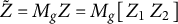 $\tilde Z = M_g Z = M_g[\,Z_1\;Z_2\,]$
reduces to
$\tilde Z = M_g Z = M_g[\,Z_1\;Z_2\,]$
reduces to
 $[\,0\;M_g Z_2\,]$
.
$[\,0\;M_g Z_2\,]$
.
The matrix
 $M_g Z_2$
has rank 1 and its column space is spanned by the neighborhood contrast
$M_g Z_2$
has rank 1 and its column space is spanned by the neighborhood contrast
 $(1,-1,1,-1)^\top $
, which alternates sign by neighborhood while being constant within each school. This is precisely the component of the neighborhood structure that is not already explained by the school-level predictor, and it is this component alone that the C-projection removes from
$(1,-1,1,-1)^\top $
, which alternates sign by neighborhood while being constant within each school. This is precisely the component of the neighborhood structure that is not already explained by the school-level predictor, and it is this component alone that the C-projection removes from
 $\tilde f$
.
$\tilde f$
.
This example illustrates two competing goals: (a) preventing the residual learner from reconstructing cluster effects already represented by the random effects and (b) preserving valid signal from group-constant predictors intentionally included in the learner.
Without projection, the learner can absorb cluster-level structure. With naive projection onto Z, valid group-constant predictor effects can also be removed. The C-projection achieves the desired compromise by preserving the span of
 $X_g$
while orthogonalizing against the residualized cluster design.
$X_g$
while orthogonalizing against the residualized cluster design.
Appendix B: Simulation study: True tree structure
True tree structure in the simulation study.

Appendix C: Paper selection for literature review on using Add Health data
Paper selection for literature review on using Add Health data.
The literature review results are posted on the Open Science Framework, https://osf.io/jkctg/.

Appendix D: Empirical study: Descriptive statistics of predictors
Descriptive statistics of predictors in the empirical study.

Note: Totals and percentages may not add up to the total sample size and 100, respectively, due to missing data and rounding. For continuous predictors, responses of “multiple response,” “does not apply,” “refused,” “don’t know,” “legitimate skip,” and “not applicable” are coded as “NA” (missing) when calculating sum scores. For categorical predictors, responses of “multiple response,” “does not apply,” “refused,” “don’t know,” “legitimate skip,” and “not applicable” are coded as “unavailable.” Predictors with the asterisk indicate sum scores of multiple predictors based on the literature.
Appendix E: Empirical study: Fixed-effect estimates of the LMMs
Fixed-effect estimates of the LMMs in the empirical study.

Note: The levels of categorical predictors are based on information available on the Add Health website and in the codebooks. Responses of “multiple response,” “does not apply,” “refused,” “don’t know,” “legitimate skip,” and “not applicable” are coded as “unavailable (9).”
Appendix F: Empirical study: Residual analyses of LMM with linear, no-interaction effects
Residual analyses of LMM.

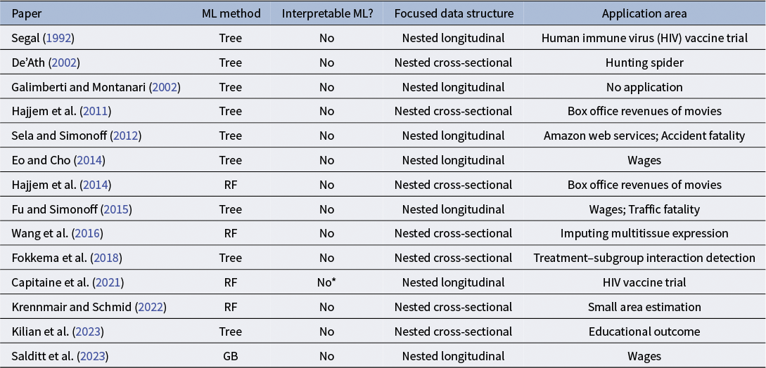
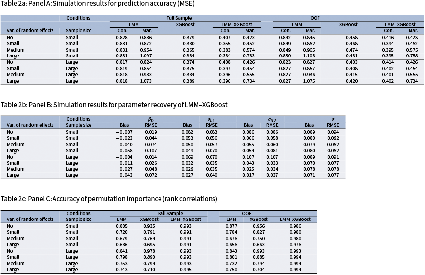
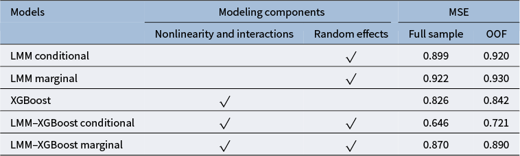
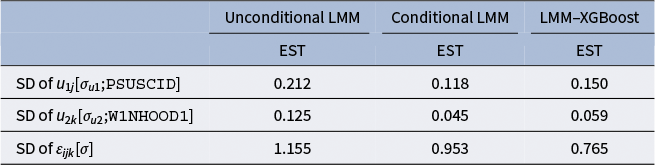
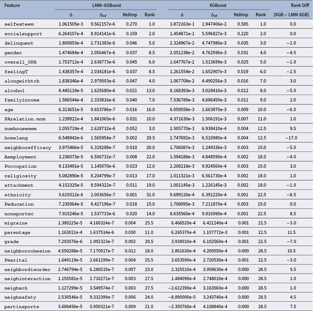
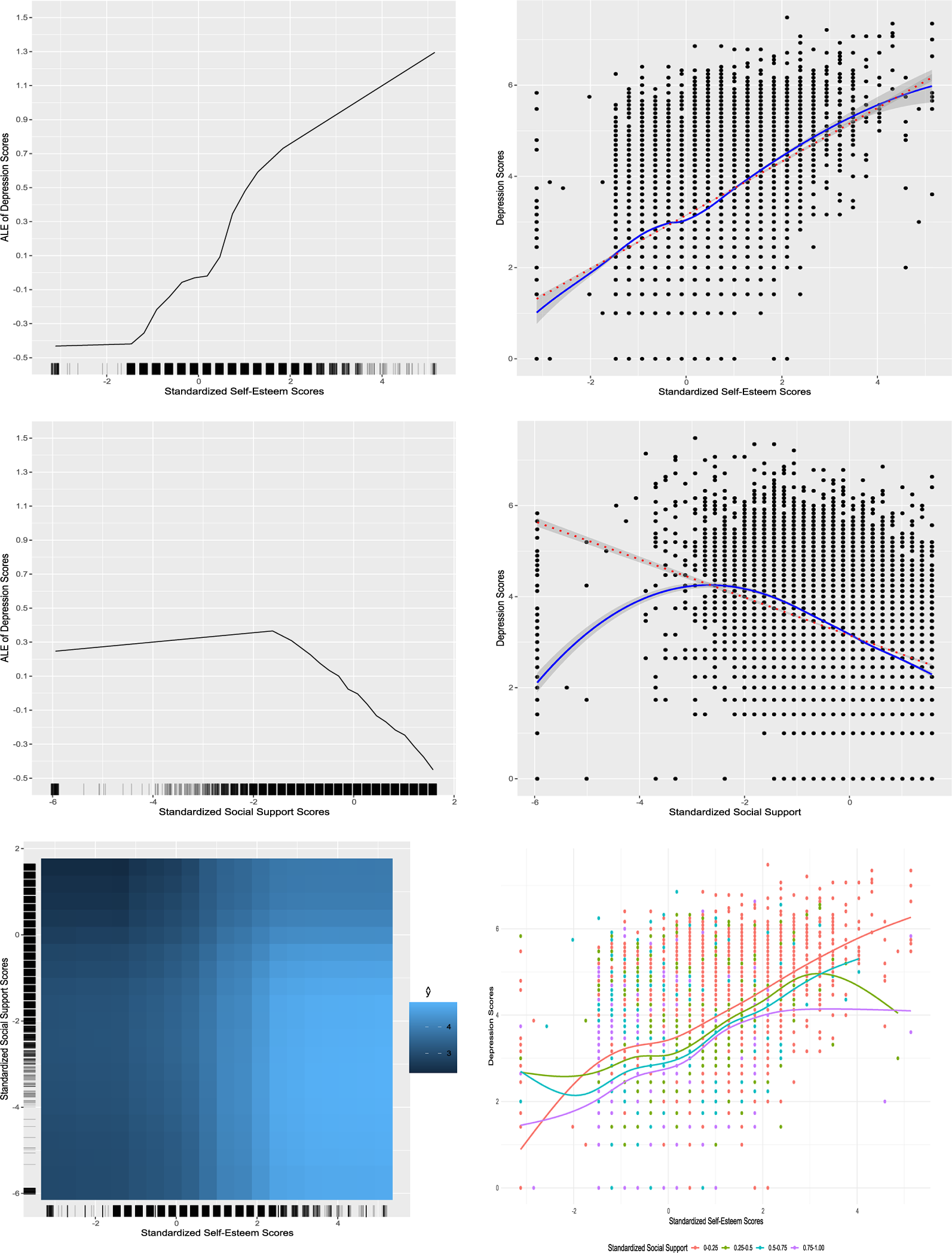
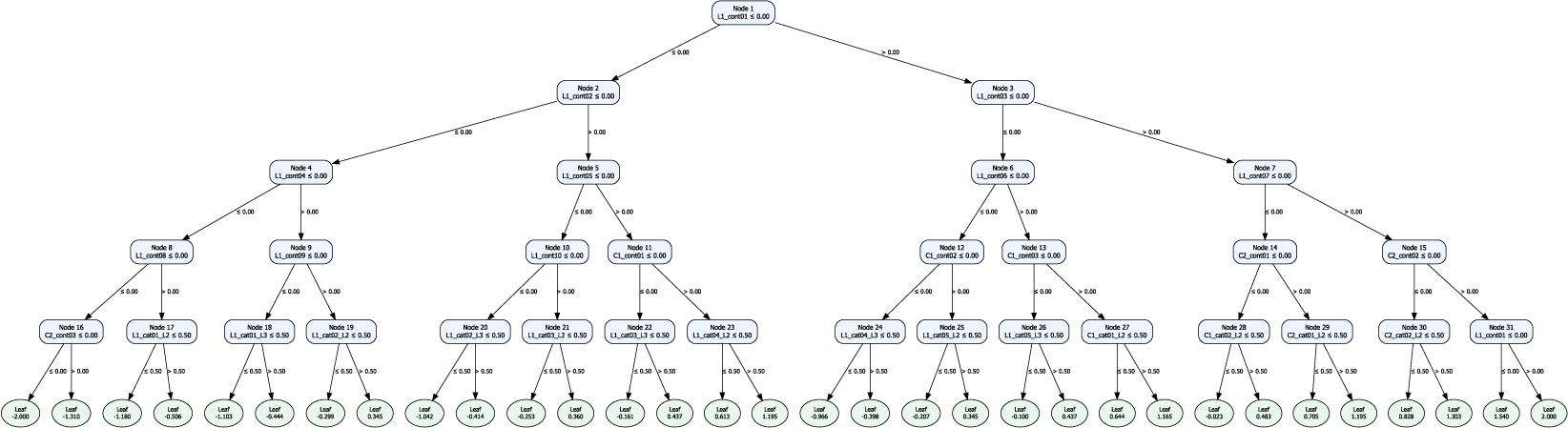
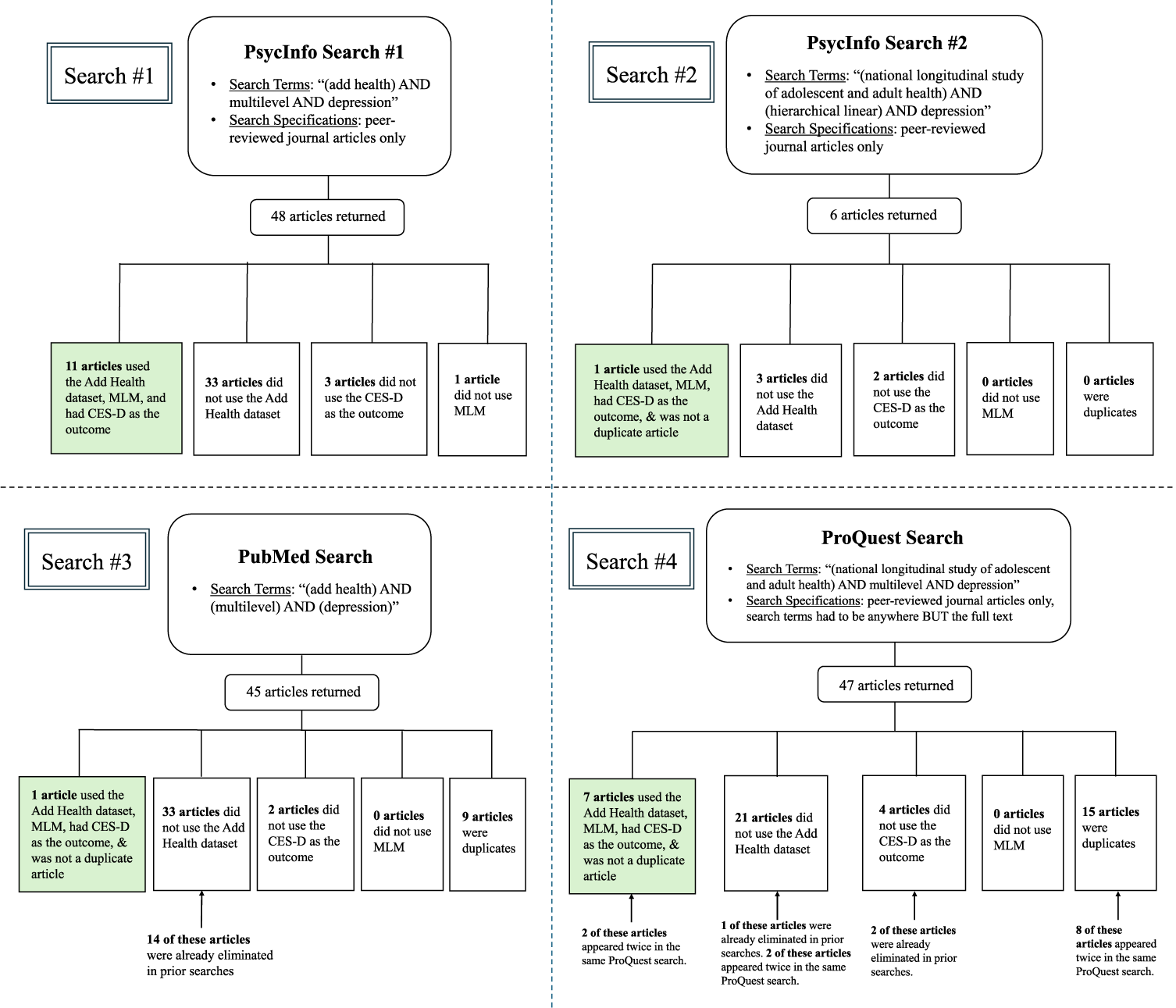
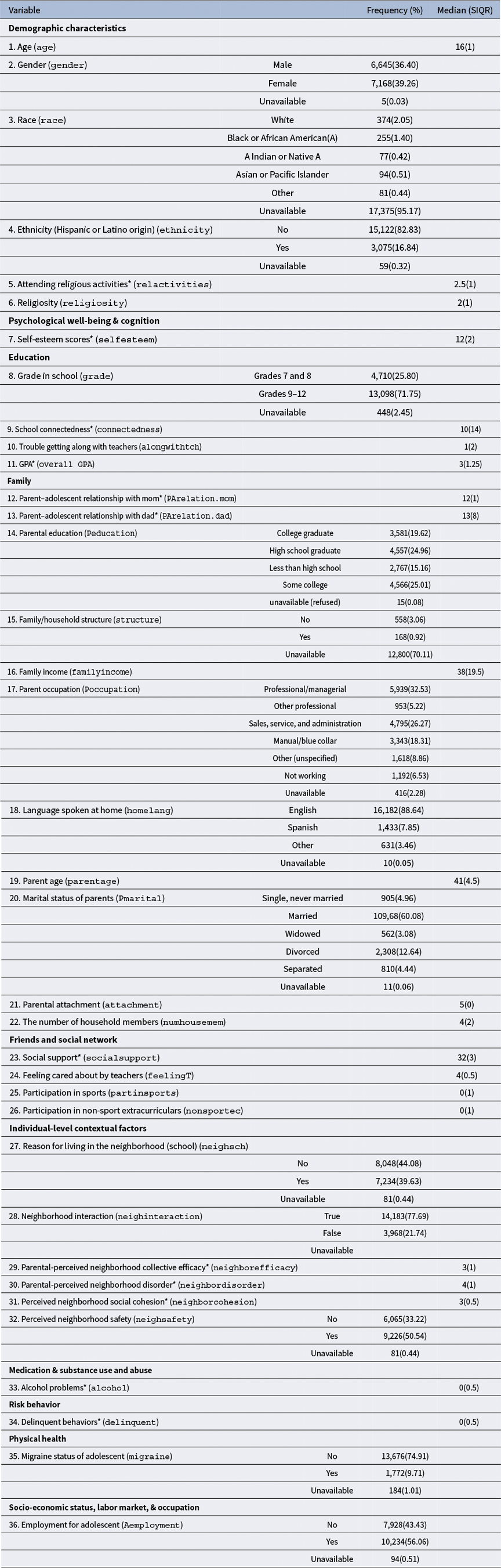
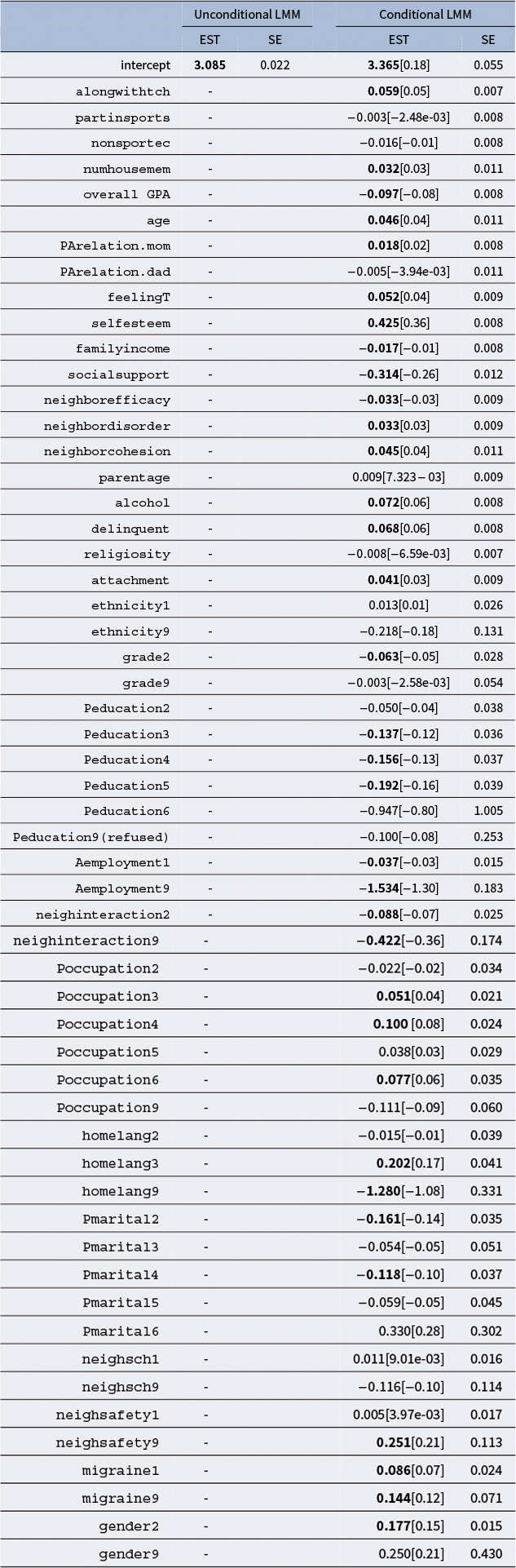
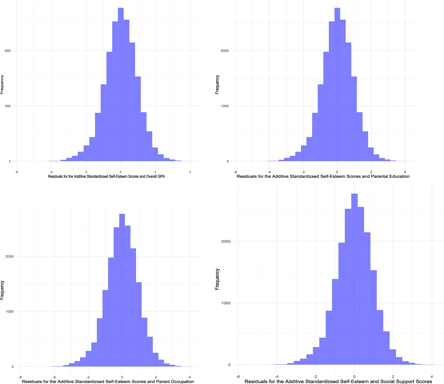

 Open access