


Introduction
Does globalization drive populism? Extensive research suggests it does: globalization shocks have fueled contemporary populist movements (for a review, see Rodrik Reference Rodrik2021). Yet, populism is not a modern phenomenon. In the United States, it emerged in the late nineteenth century (Postel Reference Postel and Dailey2022, Reference Postel2007; Slez Reference Slez2022). Nor is globalization unique to the present era; by some measures, the global economy was more integrated in the 1800s than it is today (Rodrik Reference Rodrik1997). This historical overlap raises a natural question: Did the first wave of globalization contribute to the rise of American populism?
We argue that it did. Falling transport costs from railroads and steamships deepened US integration into global markets, creating stark regional disparities in economic exposure. While international trade offered farmers the promise of expanded markets, it also exposed them to volatile commodity prices and eroded their control over local production values. Meanwhile, national political elites increasingly aligned with the industrial and urban interests of the North and East. As prices fell and financial crises struck, rural voters turned to populist parties as an alternative to the existing political establishment (Han et al. Reference Han, Milner and Mitchener2023).
To evaluate our argument, we construct a new dataset documenting county-level electoral support for populist parties in presidential, congressional, and gubernatorial elections from 1870 to 1900. We rely on the ‘big literature’ approach and classify populist parties in two ways: narrowly, as political rhetoric that frames politics as a struggle between ‘the pure people’ and ‘the corrupt elite’; and more broadly, as movements advocating nativism, anti-monopoly reforms, bimetallism, and labor rights.
We focus on the 1870–1900 period for two reasons. First, this era spans the post-Civil War transformation of the US economy, marked by rapid railroad expansion, declining transport costs, and surging exports. These developments deepened integration into global markets and heightened farmers’ exposure to international price shocks, particularly in export-oriented regions. Secondly, the same period witnessed the emergence and decline of populism – from the rise of the Grange and Greenback movements in the 1870s to the collapse of the People’s Party after William Jennings Bryan’s defeat in 1896. By 1900, many populist demands had been absorbed by the major parties, and third-party vote shares had declined sharply (Hicks Reference Hicks1931). This thirty-year window thus offers a coherent setting to examine how globalization pressures shaped mass political mobilization during the first globalization wave.
To capture counties’ exposure to international trade during the first wave of globalization, we construct a novel measure of port market access. Building on spatial trade frameworks (Donaldson and Hornbeck Reference Donaldson and Hornbeck2016; Hornbeck and Rotemberg Reference Hornbeck and Rotemberg2024), we adapt the standard market access formula by restricting destinations to counties hosting major maritime ports – the exclusive gateways for US international trade during the late nineteenth century. Each port is weighted by its total international trade volume rather than population, reflecting its role as an intermediary connecting inland producers to global demand rather than as a final consumption market. County-to-port trade costs are computed using digitized railroad, canal, and navigable waterway networks by Donaldson and Hornbeck (Reference Donaldson and Hornbeck2016). The resulting index captures a county’s ease of participation in global trade networks.
We examine the relationship between globalization and electoral populism by regressing populist vote share on the log of port market access. Across presidential, congressional, and gubernatorial elections, we find a robust positive and statistically significant relationship: counties with greater access to international trade hubs consistently exhibit higher support for populist candidates. This relationship remains stable after controlling for a range of economic, social, and demographic factors that may also shape voting behavior. A series of robustness checks confirm the consistency of our findings.
We argue that globalization affected populist support through its impact on agricultural prices. Improved access to global markets exposed farmers to international commodity price movements, intensifying competition and increasing downside risk for agricultural revenues. To evaluate this mechanism, we construct a county-level crop portfolio price index that aggregates crop-specific price changes using fixed within-county value shares, holding production quantities constant. This approach isolates revenue exposure to global price movements from endogenous changes in output composition.
We show that greater port market access is associated with declining agricultural portfolio prices and that the political effects of globalization are strongest in counties initially specialized in crops that experienced the largest national price declines. These findings suggest that inexorable exposure to adverse global price shocks – rather than endogenous adjustment – was a central channel linking globalization to populist mobilization.
This paper contributes to a growing literature on the political consequences of the first wave of globalization. First, we build on Eichengreen et al. (Reference Eichengreen, Haines, Jaremski, Leblang, Hanes and Wolcott2019) and Klein et al. (Reference Klein, Persson and Sharp2023), who document the role of economic dislocation in driving populist voting during the 1890s. Eichengreen et al. (Reference Eichengreen, Haines, Jaremski, Leblang, Hanes and Wolcott2019) link Bryan’s 1896 vote share to crop price declines, limited rail access, and high rural interest rates, showing that local economic hardship could meaningfully shape national electoral outcomes. Klein et al. (Reference Klein, Persson and Sharp2023) emphasize that counties facing higher transportation costs to international hubs like New York City and Chicago – particularly those on the agrarian frontier – exhibited stronger support for the People’s Party in the 1892 presidential election.
Our paper advances this literature in three key respects. First, rather than focusing on a single election, we construct a county-level panel across presidential, congressional, and gubernatorial races between 1870 and 1900 to analyze broader electoral dynamics. Secondly, we move beyond proxies like wheat prices or rail density by constructing a structural measure of port market access that captures a county’s integration into international trade networks. Thirdly, we identify and empirically test a specific mechanism – heightened exposure to global price shocks – that links port market access to populist voting. In doing so, we show that globalization not only transmitted economic risk into rural America but also transformed that risk into populist political mobilization.
Secondly, we complement and extend the analysis in Scheve and Serlin (Reference Scheve and Serlin2025), who argue that falling transportation costs reshaped political coalitions in the United States by inducing population shifts and altering local economic interests. They show that reduced costs of shipping goods to the nearest of eleven major ports led to economic growth and declining support for free-trade Democrats, fueling protectionist sentiment. We build on their methodological insight – that spatial variation in access to trade infrastructure shapes political outcomes – but take a broader approach in both scope and intent. We construct a measure of port market access that incorporates US ports operating during the period, weighting them by international trade volume and adjusting for trade elasticities. This allows us to capture a county’s overall ease of participation in global trade networks, rather than access to a single export node. By leveraging this richer measure, we show that global integration, even in the absence of direct urban or industrial growth, increased local economic volatility and fueled populist backlash.
Thirdly, our findings also build on Chan (Reference Chan2025), who documents that trade booms during the first wave of globalization spurred population growth and manufacturing expansion in US port districts, but that these benefits dissipated rapidly with distance. Counties adjacent to ports – though geographically close – did not share in the economic gains, highlighting the sharply uneven spatial distribution of globalization’s rewards. Our work demonstrates that the uneven economic consequences of globalization can also produce uneven political responses – a dynamic that connects the geography of trade to the geography of political backlash.
Economic Causes of the American Populist Movement
The late-nineteenth-century populist movement was one of the largest mass mobilizations in US history, emerging in response to the dislocations of post-Civil War economic development (Hahn Reference Hahn2006; Slez Reference Slez2022; Smångs and Redding Reference Smångs and Redding2019). During this period, politically oriented coalitions of American ‘farmers, wage earners, women, and other sectors of society’ mobilized and advocated for their equal standing (Postel Reference Postel and Dailey2022). These efforts coalesced through successive organizational waves: the Grange and the Greenbacks in the 1870s, the Farmers’ Alliance in the 1880s, and the People’s Party in the 1890s (Hicks Reference Hicks1931; Judis Reference Judis2016; McMath Reference McMath1993).
Scholars have long debated the economic origins of the late-nineteenth-century populist movement. While scholars broadly agree that economic grievances played a central role, they disagree on the precise mechanism: some emphasize persistent material hardship, while others point to rising economic uncertainty as the primary catalyst for mobilization.
Progressive historians argue that a prolonged decline in commodity prices, restricted access to credit and currency, exploitative railroad monopolies, and burdensome debt drove farmers towards revolt (Buck Reference Buck1913; Hicks Reference Hicks1931; Woodward Reference Woodward2014). These conditions, they suggest, enabled intermediaries – so-called ‘middlemen’ – to exert disproportionate economic and political power, thereby depriving rural producers of their rightful share of national prosperity (Pollack Reference Pollack1967). Supporting this perspective, Eichengreen et al. (Reference Eichengreen, Haines, Jaremski, Leblang, Hanes and Wolcott2019) show that counties experiencing sharper crop price declines awarded greater vote shares to William Jennings Bryan in the 1896 presidential election.
Yet this interpretation has not gone unchallenged. Some scholars, most notably Douglass North, argue that farmers may have misperceived the severity of their economic conditions. North (Reference North1974) maintains that while nominal farm prices fell, real agricultural prices remained largely stable, and the terms of trade for farmers even improved during this period. On transportation costs – a frequent populist complaint – both North (Reference North1974) and Aldrich (Reference Aldrich1980) document stable or broadly declining railroad freight rates between 1865 and 1900.
If economic conditions were not unequivocally deteriorating, why did farmers so fervently join the populist revolt? An alternative literature points to increasing volatility and perceived unfairness rather than declining averages. As Higgs (Reference Higgs1971) points out, American farmers faced a wide array of unpredictable and often devastating risks that generated significant year-to-year fluctuations in yields and income. These natural hazards contributed to an acutely unstable economic environment. Klein et al. (Reference Klein, Persson and Sharp2023) argue that farmers, particularly those located further from major export hubs, perceived the high transportation costs charged by rail companies and middlemen as unfair.
Moreover, a defining feature of late-nineteenth-century agriculture was its transformation into a largely commercialized sector. Increasingly integrated into global commodity markets, farmers lost pricing power over their undifferentiated crops and became more vulnerable to volatile international demand and supply shocks (Mayhew Reference Mayhew1972). Populist supporters included not only subsistence farmers but also highly market-exposed producers whose livelihoods rose and fell with global price fluctuations (McMath Reference McMath2008). Indeed, Higgs (Reference Higgs1971) and Parker (Reference Parker and Davis1972) argue that this heightened exposure to market risks – rather than absolute deprivation – served as a powerful driver of populist sentiment. Consistent with this view, McGuire (Reference McGuire1981) finds that various indicators of agricultural instability strongly predict rural unrest in fourteen northern states from 1866 to 1909. Similar patterns appear in Kansas (DeCanio Reference DeCanio1980) and other midwestern states (Stock Reference Stock1984).
A Theory of Globalization and American Electoral Populism
The late nineteenth century marked a period of dramatic economic transformation in the United States, commonly referred to as the first wave of globalization (Meissner Reference Meissner2024). Expanding railroads, steamships, and telegraph networks connected distant markets, facilitated international trade, and transformed the economic landscape (Postel Reference Postel2007). As the nation shifted from an agrarian to an industrial economy – especially in the North and East – rural farmers increasingly felt sidelined by policies favoring industrial and financial elites, giving rise to influential populist movements.
Theoretical Expectations of Globalization
Classical trade theory contends that globalization benefits a country’s abundant factors of production. According to the Stolper–Samuelson theorem, trade raises the real returns to the abundant factor while lowering the returns to the scarce factor (Stolper and Samuelson Reference Stolper and Samuelson1941). In the nineteenth-century United States – abundant in land but scarce in labor and capital – this implies that increased trade would boost demand for farm products, elevating land values and farmers’ incomes. Building on Ricardo (Reference Ricardo1817), comparative advantage theory likewise predicts that the United States would export agricultural goods and import manufactured products, driving up domestic agricultural prices.
Evidence supports the integration of global commodity markets during this period. O’Rourke et al. (Reference O’Rourke, Taylor and Williamson1996) document significant price convergence between Europe and the United States, indicating that globalization should have bolstered American agricultural prices. Jacks et al. (Reference Jacks, Meissner and Novy2011) further illustrate that reductions in transportation costs led to increased trade volumes and market integration. Theoretically, these developments would position farmers as primary beneficiaries of globalization, reaping rewards from increased demand and higher prices for their products.
The Paradox of Declining Agricultural Prices
Yet, despite these forecasts, American farmers confronted falling agricultural prices and worsening economic conditions (North Reference North1966; Schwartz and Friedman Reference Schwartz and Friedman1963). Several interrelated factors contributed to this paradox, complicating the direct application of the Stolper–Samuelson theorem.
First, global oversupply weighed heavily on prices. Newly opened agricultural frontiers in Canada, Argentina, Australia, and Russia produced surpluses of staple commodities like wheat and corn (Findlay and O’Rourke Reference Findlay and O’Rourke2007). This surge in supply outpaced the growth in global demand, exerting downward pressure on international commodity prices. As global markets became saturated, even countries with a comparative advantage in agriculture faced stiff competition, undermining the expected gains from trade. Williamson (Reference Williamson2006) notes that the late nineteenth century saw a ‘commodity price convergence’ that was not necessarily beneficial to all producers.
Secondly, domestic trade policies compounded farmers’ problems. High protective tariffs – averaging 40–50 per cent after the Morrill Tariff of 1861 – shielded American manufacturers from foreign competition (Irwin Reference Irwin2007, Reference Irwin2020). Farmers, meanwhile, faced steeper prices for manufactured inputs (Gourevitch Reference Gourevitch1977) and endured retaliatory tariffs on their exports (Taussig Reference Taussig1910). As Harley (Reference Harley1992) observes, ‘the tariff reduced American imports and in turn reduced the export of foodstuffs. The main costs of the tariff thus fell on land, as the factor used intensively in food production. The West, as well as the South, were the principal losers from the protection of manufacturing’. This mismatch in policy favored industrial interests at the expense of farmers, defying Stolper–Samuelson’s expectation that the abundant factor (land) would reap the benefits of trade.
Thirdly, macroeconomic choices – particularly adherence to the gold standard – created a deflationary environment. As general price levels fell, farmers’ real debt burdens increased (Schwartz and Friedman Reference Schwartz and Friedman1963). Lower nominal incomes combined with fixed loan obligations pushed many deeper into debt (North Reference North1974).
Additionally, globalization exposed farmers to greater price volatility and market risks. Deeper integration made them vulnerable to abrupt shifts in global supply and demand (Allen and Atkin Reference Allen and Atkin2022), yet they lacked effective hedging tools or leverage over international prices (Atack and Bateman Reference Atack and Bateman1987). Consequently, income fluctuations became more unpredictable, exacerbating farmers’ economic insecurity.
Farmers’ Grievances and the Emergence of Populism
Despite straining the agricultural sector, globalization facilitated America’s Second Industrial Revolution by unlocking foreign capital, technology, and markets (Chandler Reference Chandler1977; James Reference James1978). Northern and eastern cities grew rapidly, propelled by industrial expansion, technological innovation, and immigration (Mogford and Hirschman Reference Mogford and Hirschman2009; Mokyr Reference Mokyr1992; Nelson et al. Reference Nelson, Wright and Nelson1992).
Politically, the Republican Party (dominant from 1861 to 1932) was closely aligned with industrial and financial interests (Bensel Reference Bensel2000). Its policies of high tariffs, strict adherence to the gold standard, and unregulated railroad expansion prioritized industry over agriculture. Although the Homestead Act and railroad land grants encouraged westward settlement, they also led to monopolistic practices and speculative abuses (McGuire Reference McGuire1981, Reference McGuire1982). These policies deepened the urban–rural divide, leaving many farmers feeling marginalized by a government seemingly beholden to urban industrialists (Goodwyn Reference Goodwyn1978).
Declining commodity prices, increased debt burdens, and volatile global markets ignited widespread farm unrest (Clanton Reference Clanton1998; Hicks Reference Hicks1931). Farmers also grappled with monopolistic practices among railroad companies and grain elevator operators, who charged high fees and discriminatory rates in rural areas lacking real competition (Chandler Reference Chandler1977). Although the Interstate Commerce Act of 1887 attempted to address some of these issues, it was only partially effective (Miller Reference Miller1971).
Credit constraints further exacerbated farmers’ financial vulnerability. Rural financial markets were underdeveloped, forcing farmers to rely on local lenders charging high interest rates (Eichengreen Reference Eichengreen1984). The National Banking Acts of 1863 and 1864 centralized banking in urban areas, further restricting rural credit access (James Reference James1978). Farmers, faced with income instability and expensive loans, struggled to invest in technology or weather prolonged low-price intervals.
In response, populist movements emerged, advocating for policies to alleviate farmers’ economic distress (Goodwyn Reference Goodwyn1978; Postel Reference Postel2007). Populist parties condemned the influence of industrial and financial elites, advocating for bimetallism (the free coinage of silver) to generate moderate inflation and reduce debt burdens, along with public regulation or ownership of railroads and grain storage. Populists additionally sought to democratize political and economic institutions, advocating for stronger rural representation, direct senatorial elections, and broader citizen engagement in governance.
Connecting Globalization to Populist Support
The link between globalization and populist support lies in the differential impact of global economic integration on various regions and sectors. Counties more exposed to globalization – through higher levels of agricultural production for export or greater reliance on global commodity markets – experienced the adverse effects more acutely. These areas faced economic hardship due to declining commodity prices and increased competition, as well as heightened market vulnerabilities from exposure to international price fluctuations and supply shocks. These economic pressures were compounded by national policies prioritizing industrial interests, which often marginalized rural agrarians (Bensel Reference Bensel2000). High tariffs and commitment to the gold standard, among other measures, favored urban industrialists while offering little relief to farmers, thus fueling rural discontent.
Empirical studies in contemporary settings find that regions adversely affected by globalization are more likely to exhibit increased support for populist or anti-establishment parties (for a review, see Rodrik Reference Rodrik2021). While these studies focus on modern contexts, the underlying mechanisms are applicable to the historical setting of late-nineteenth-century America. The economic hardships induced by globalization can lead to political realignment and increased support for movements that challenge the status quo.
HYPOTHESIS 1: Counties more exposed to globalization will show higher support for populist parties in the late-nineteenth-century United States.
American Populists, 1870–1900: A New Database
The natural next step is to systematically examine the rise and fall of populist parties in late-nineteenth-century American politics. Yet, no comprehensive dataset is currently available. Classifying prominent parties such as the People’s Party as populist is relatively straightforward, but the process is more complex for minor and ‘fusion’ parties. To address these inconsistencies, we develop a consistent, rule-based classification of populist parties over time. This approach allows us to construct a new dataset that traces the evolution of electoral populism across US counties during this period.
Defining Populism
We adopt two working definitions of populism. The first is a ‘thin’ ideological definition commonly used in political science; the second is a broader, historically grounded version tailored to the late-nineteenth-century American context.
Under the ‘thin’ definition, populism is an ideology defined by two core ideas: (1) society is composed of homogeneous and antagonistic groups, ‘the pure people’ versus ‘the corrupt elite’; and (2) politics should directly reflect the general will of the people (Mudde Reference Mudde2004). The claim is that society has been led astray by corrupt elites who have distorted the economy to serve their interests, betraying the will of the people by accepting new cosmopolitan values and behavior. This definition includes anti-pluralism but focuses much less on exclusionary identity politics than the definition of Müller (Reference Müller2016).Footnote 1 Crucially, populists do not merely critique elites; they claim an exclusive right to speak for the ‘true’ people of the nation.
Beyond its ‘thin’ dimension, populism often extends beyond this thin core to incorporate nativist, nationalist, or xenophobic themes (Hawkins Reference Hawkins2009; Hawkins and Littvay Reference Hawkins and Littvay2019; Mudde Reference Mudde2004). They promoted a nostalgic desire to return to a purer age and set of values that give priority to the nation and are less contaminated by new, foreign, cosmopolitan values and behaviors.
In the late-nineteenth-century United States, populist movements advanced a broad reform agenda that extended beyond the ideological core of populism. Their platform emphasized anti-monopoly regulation, monetary reform, and labor rights in response to emerging social and economic pressures.
First, populists challenged the power of monopolies by supporting public regulation or ownership of railroads and grain elevators. They advocated equitable freight rates and organized co-operative enterprises, including large-scale trading companies designed to bypass merchant houses in domestic and transatlantic markets (Postel Reference Postel and Dailey2022).
Secondly, populists rejected the gold standard, advocating instead for greenbacks or free silver. They argued that a shift to a depreciated silver standard – or a floating paper currency – would raise prices for export commodities like wheat, cotton, and minerals, which were otherwise unprotected by tariffs (Frieden Reference Frieden1997).
Thirdly, they endorsed key labor demands, including a shorter workday and the enforcement of the eight-hour rule for public employment. Their platform also called for institutional reforms aimed at curbing corruption and enhancing democratic accountability, such as civil service reform, the direct election of Senators, the secret ballot, and mechanisms for referendum.
Classifying Voting Data in the Inter-university Consortium for Political and Social Research (ICPSR) 1
To examine electoral populism at both the federal and state levels between 1870 and 1900, we construct a new dataset of election outcomes. The dataset draws from the ICPSR 1: United States Historical Election Returns (1824–1968) (ICPSR 1999), the most comprehensive source of US historical election results currently available.
Our analysis focuses on presidential, House, and gubernatorial elections. We exclude Senate contests because the 17th Amendment (instituting direct senatorial elections) was not adopted until 1913. Across these elections, we identify 310 unique parties that received votes in at least one contest. For thirty-one of these parties, no party name is recorded in ICPSR’s ‘DS204 – Political Party Codes’ file. We contacted the ICPSR in February 2024, but they were unable to provide further details. Given the low frequency and negligible combined vote shares of these unnamed parties, we do not expect this omission to materially affect our analysis.
Following the ‘big literature’ approach used by Milner (Reference Milner2021) and Funke et al. (Reference Funke, Schularick and Trebesch2023), we code each of the 279 identifiable parties in our sample as populist (=1) or non-populist (=0). Classifications are based on published scholarship spanning the last 150 years, including books, book chapters, and peer-reviewed articles focused on American populism. For minor parties with limited documentation, we supplement the literature with historical newspaper coverage.Footnote 2
We implement two classification strategies – narrow and broad – based on the definitions outlined above. The narrow approach applies stringent criteria, coding a party as populist only if it meets both core conditions of the ‘thin’ definition: anti-elite rhetoric and claims to exclusive representation of the people. The broad approach adopts a more inclusive standard, identifying parties as populist if they employed nativist rhetoric or endorsed policy positions commonly associated with nineteenth-century populism, such as anti-monopoly reform, opposition to the gold standard, or support for labor rights.
Of the 279 parties in our sample, 65 are classified as populist under the narrow definition and 108 under the broad definition (see Appendices B.1 and B.2).
American Electoral Populism: 1870–1900
We begin by examining the electoral performance of populist parties from 1870 to 1900, plotting their vote shares in presidential, House, and gubernatorial elections. Figures 1–3 show results using a narrow definition of populism, while Figures B.1–B.3 report analogous trends under a broader classification.
Populist vote share in presidential elections, 1870–1900.
Note: authors’ calculation based on the ICPSR 1: United States Historical Election Returns, 1824–1968 (ICPSR 1999). The populist party is narrowly defined; see Appendix B.1 for a full list. The vote share refers to the national share of votes cast for populist parties. For the broadly defined populist classification and corresponding trend, see Appendices B.2 and B.3.

Populist vote share in house elections, 1870–1900.
Note: authors’ calculation based on the ICPSR 1: United States Historical Election Returns, 1824–1968 (ICPSR 1999). The populist party is narrowly defined; see Appendix B.1 for a full list. The vote share refers to the national share of votes cast for populist parties. For the broadly defined populist classification and corresponding trend, see Appendices B.2 and B.3. Voting data of odd-year specials were excluded.

Populist vote share in gubernatorial elections, 1870–1900.
Note: authors’ calculation based on the ICPSR 1: United States Historical Election Returns, 1824–1968 (ICPSR 1999). The populist party is narrowly defined; see Appendix B.1 for a full list. The vote share refers to the national share of votes cast for populist parties. For the broadly defined populist classification and corresponding trend, see Appendices B.2 and B.3.

As an initial validation step, we assess consistency across coding schemes. The Pearson correlation between the two series is high – 0.99 for presidential elections and 0.96 for House and gubernatorial races – indicating strong alignment across definitions. At the national level, the mean difference in vote share between the two measures remains modest: 0.65 percentage points for presidential elections, 1.50 for House, and 0.91 for gubernatorial races. These results suggest that our main findings are robust to alternative definitions of populism.
All three figures reveal a bimodal distribution in populist vote shares: a modest rise in the late 1870s and early 1880s, followed by a more pronounced surge in the 1890s. Populist parties consistently performed best in gubernatorial elections, followed by House contests, with the lowest vote shares in presidential races. This hierarchy suggests that populist strength was often rooted in localized or regional constituencies, translating into relatively stronger performance in subnational elections. The gubernatorial advantage may reflect more effective state-level organization, while the weaker presidential performance likely reflects the difficulty of building a viable national coalition under the prevailing electoral system.
Next, we examine the spatial distribution of populist support during two high points in their electoral performance: the 1892 presidential election and the 1894 House and gubernatorial contests (Figures 4–6). While populist vote shares varied over time, these elections represent moments when populist parties competed nationally under their own label and received substantial support. Across all three maps, populist strength was concentrated in the Mountain West, parts of the South, and sections of the Plains, while the industrial Northeast showed limited populist presence.
County-level populist vote share in the 1892 presidential election.
Note: authors’ calculation based on the ICPSR 1: United States Historical Election Returns, 1824–1968 (ICPSR 1999). The populist party is narrowly defined; see Appendix B.1 for a full list. The map blackens Virginia because the ICPSR1 dataset does not report voting outcomes for the state between 1889 and 1892. The color scale uses a diverging palette centered at 10 per cent.

County-level populist vote share in the 1894 house election.
Note: authors’ calculation based on the ICPSR 1: United States Historical Election Returns, 1824–1968 (ICPSR 1999). The populist party is narrowly defined; see Appendix B.1 for a full list. The color scale uses a diverging palette centered at 10 per cent.

County-level populist vote share in the 1894 gubernatorial election.
Note: authors’ calculation based on the ICPSR 1: United States Historical Election Returns, 1824–1968 (ICPSR 1999). The populist party is narrowly defined; see Appendix B.1 for a full list. In 1894, twenty-eight states held gubernatorial elections. The map blackens states where no gubernatorial election happened in that year. The color scale uses a diverging palette centered at 10 per cent.

Measuring Globalization Using Port Market Access
To estimate counties’ exposure to globalization during the late nineteenth century, we adapt the standard market access measure frequently employed in spatial trade models. Following Donaldson and Hornbeck (Reference Donaldson and Hornbeck2016) and Hornbeck and Rotemberg (Reference Hornbeck and Rotemberg2024), a county’s market access is defined as a weighted sum of destination populations, where each destination is inversely weighted by the cost of transporting goods to that destination, raised to a trade elasticity parameter:
 $$\textrm {MA}_o = \sum _{d \neq o}(\tau _{od})^{-\theta } L_d$$
where τ
od
denotes the bilateral ‘iceberg trade cost’ between the origin county o and the destination county d, which normalizes the measured per-ton county-to-county transportation costs by the average price per ton of transported goods ( $\tau _{od} = 1 + t_{od}/\overline {P}$
), θ is the ‘trade elasticity’, and L
d
is the population of destination county d, serving as a proxy for market size.
$\tau _{od} = 1 + t_{od}/\overline {P}$
), θ is the ‘trade elasticity’, and L
d
is the population of destination county d, serving as a proxy for market size.
We modify this framework to focus on international rather than domestic market integration. Our port market access measure, denoted Port MA o , is constructed as:
 $${\rm Port\;MA}_o = \sum _{p \neq o}(\tau _{op})^{-\theta } T_p$$
where p denotes the set of destination counties containing major maritime ports and T p is the total volume of international trade (imports plus exports) handled by p.
Equation (2) deviates from Equation (1) in two key dimensions: (1) the restriction of the destination set exclusively to port counties, and (2) the weighting of these destinations by trade volume rather than population. We detail the theoretical and empirical rationale for each modification below.
First, we restrict the summation to include only destination counties that hosted major ports – the nodes through which international trade occurred. Theoretically, while the logic of market access applies to any defined set of destinations, our specific interest lies in how access to global markets shaped the political economy of populism. By isolating port counties, we capture a county’s potential to engage in international trade – specifically, the ability to ship agricultural products abroad and import foreign goods. This contrasts with broader market access measures, which include all domestic counties and consequently confound specific globalization exposure with general domestic market integration.
Empirically, this restriction is consistent with the mechanics of the first wave of globalization. During this period, US exports of wheat, cotton, and other agricultural commodities expanded rapidly, fueled by declining transport costs and rising foreign demand. Port counties served as the exclusive gateways for this trade. Therefore, counties with better transport connectivity to these specific nodes were uniquely exposed to international price signals, global demand shocks, and foreign competition. We note, however, that major port cities were also the largest domestic population centers. Consequently, our port market access measure captures exposure to a ‘bundle’ of market forces: both the direct opportunity to export agricultural goods abroad and the access to deep domestic markets.
Secondly, we weight each destination port by its total international trade volume (T p ) rather than its population (L p ). Standard market access measures utilize population as a proxy for market size, which is appropriate when modeling domestic consumption demand. However, in the context of international trade, ports function as intermediaries rather than final consumption destinations. A port’s relevance to an inland producer is defined by its capacity to channel goods to and from global markets, a characteristic that is not necessarily correlated with its local population.
Using international trade weights corrects for potential measurement error where population poorly proxies for a port’s role in the global economy. For example, while New York City handled over half of all US international trade during much of our sample period (Ellis Reference Ellis1952), it contained a significantly smaller fraction of the US population. Therefore, a population-weighted measure would severely downweight New York’s distinct role as the primary conduit for nineteenth-century globalization.
We construct the dataset of port-level trade volumes using The Foreign Commerce and Navigation of the United States. Published annually by the US government, this series constitutes the official historical record of US trade with the world.
We leverage the recent digitization of these records by Chan (Reference Chan2025) as our primary data structure. To ensure accuracy and consistency with our specific definitions, we independently cross-referenced the digitized entries against the original statistical tables available via the HathiTrust Digital Library. Our verification process confirmed the integrity of the series across our three census years (1870, 1880, and 1890).
We define the trade volume (T p ) for each port as the sum of general imports and domestic exports. We explicitly exclude ‘re-exports’ (foreign merchandise exported in the same condition as imported). This distinction is theoretically crucial: re-exports represent transshipment activity that does not originate from US producers. By focusing on domestic exports, our measure captures the direct integration of the American interior with foreign demand shocks.
The original data was reported at the customs district level, a federal administrative unit created by Congress for customs duty collection. To integrate these administrative units into our spatial analysis, we map each customs district to a unique county based on the location of its principal ‘port of entry’ – the federally designated location where foreign merchandise was legally entered and appraised.
For the vast majority of observations, a customs district contains a single dominant port of entry, allowing for a precise one-to-one mapping to a county. In four exceptional cases where a customs district spans multiple distinct economic centers or counties, we apportion the district-level trade volume to the constituent counties based on their share of total wealth (real estate and personal property) as reported in the decennial census.Footnote 3 This follows the apportionment methodology established in Donaldson and Hornbeck (Reference Donaldson and Hornbeck2016) for handling imperfect spatial matches.
To account for the entry and exit of ports, the set of destination ports is dynamic: a county is included in the calculation for a given decade if and only if its customs district reported positive trade flows in that year. This approach prevents the attribution of market access to locations that were not yet operational or had ceased international commerce.
We construct port market access (Port MA
o
) at the decade level (1870, 1880, and 1890). The construction of port market access follows standard procedures. We use county-to-county transportation cost data (τ
op
) constructed by Donaldson and Hornbeck (Reference Donaldson and Hornbeck2016), which are based on shortest-cost freight routes linking county centroids through digitized railroad, canal, and navigable waterway networks.Footnote
4
Following Hornbeck and Rotemberg (Reference Hornbeck and Rotemberg2024), we estimate a trade elasticity of θ = 3.05 and normalize trade costs using an average goods value of $\overline {P} = 38.7$
.
$\overline {P} = 38.7$
.
This port-based measure offers several advantages. First, by restricting destinations to major ports, it isolates variation in access to international markets rather than domestic market integration. Secondly, weighting ports by international trade volumes ties the measure to global demand conditions rather than local consumption, improving its relevance for studying globalization exposure. Thirdly, the measure preserves the theoretical structure and interpretability of standard market access frameworks, ensuring comparability with existing work in spatial trade and economic geography.
As in the broader market access literature, we do not interpret port market access as providing a fully exogenous source of variation. Transportation networks, economic development, and political outcomes may be jointly determined over longer horizons. Accordingly, our empirical results are best interpreted as documenting reduced-form relationships between differential exposure to international markets and local political outcomes. We view this reduced-form relationship as complementary to the existing literature on globalization and political behavior, which often emphasizes exposure measures rather than plausibly exogenous shocks when studying long-run political outcomes.
We examine the spatial distribution of port market access and its connection to populist electoral outcomes. Figure 7 shows the change in log port market access between 1870 and 1890. The largest increases are concentrated in the central Great Plains – particularly Nebraska, Kansas, and parts of the Dakotas – where counties became substantially more integrated into export networks via expanding transportation infrastructure. When compared to Figures 4–6, a clear spatial correspondence emerges: counties with greater improvements in port connectivity tend to align with areas of stronger populist support. This geographic overlap provides suggestive evidence that rising access to global markets was associated with heightened populist mobilization – a relationship we explore more formally in the regression analysis.
Change in log port market access between 1870 and 1890.
Note: authors’ calculations.

Data and Empirical Strategy
To test our hypothesis, we estimate the following equation: ${\rm{PopulistShar}}{{\rm{e}}_{c,t}} = {\beta _0} + {\beta _1}{\rm{ln}}({\rm{Port}}\;{\rm{M}}{{\rm{A}}_{c,t}}) + {\beta _2}Z'c,t + {\alpha _c} + {\alpha _t} + {\epsilon_{c,t}}$
where c denotes counties and t denotes years. The dependent variable, PopulistShare c, t , is the vote share received by populist parties in presidential, congressional, or gubernatorial elections in year t. The main explanatory variable, ln(Port MA c,t ), is the natural logarithm of county-level port market access in the decade encompassing year t. Z′ c, t is a vector of time-varying county characteristics, while α c and α t denote county and year fixed effects, respectively. Standard errors are clustered at the county level. Under our hypothesis, we expect β 1 > 0. The analysis in the main body adopts a narrow definition of populism; results using an alternative, broader classification are reported in Appendix D.
To account for potential confounders identified in the literature, we include Z′ c, t , a vector of demographic and sectoral controls, along with a third-degree polynomial in the length of railroad track within forty miles of the county centroid, f(RailLength c,t ). These variables capture local economic structure, demographic composition, and financial conditions that may be correlated with both port market access and political preferences. Including this set of controls allows us to assess whether the relationship between port market access and populist voting persists after accounting for alternative channels emphasized in prior work.
Bank monopoly
Populist parties drew strong support from farmers and ranchers who often faced limited access to credit in rural areas. To account for variation in financial constraints, we control for banking penetration using county-level data from Jaremski and Fishback (Reference Jaremski and Fishback2018), who digitized historical directories to construct the first nationwide bank database at the county level between 1870 and 1900. We measure the number of banks per 1,000 residents (lagged one year) as a proxy for local access to credit. This variable may confound the relationship between port market access and populist support if areas with better connectivity also had more competitive banking sectors.
Gold and silver production
The free coinage of silver was a central theme of populist platforms, especially in the West, where silver symbolized monetary expansion and ‘economic justice’.
To capture local economic interests tied to bimetallism, we construct county-level measures of gold and silver production. State-level annual production figures are sourced from the Statistical Abstract of the United States. Because substate production data are unavailable (Rothwell Reference Rothwell1892), we apportion state-level output to counties using each county’s share of state mining employment. Mining employment is measured using full-count Census microdata, which we use to proxy for the spatial distribution of extractive activity within states. Because the 1890 Census was largely destroyed by fire, we rely on mining employment from the 1880 Census as a proxy for county-level mining activity in 1890.
Specifically, for each state-year, we apportion total gold and silver output to counties in proportion to their mining employment shares, assuming that production intensity scales with labor inputs across locations. We then take the logarithm of the resulting county-level estimates and lag them by one year.
Other industry and demographic controls
We also include a set of time-varying county characteristics that may shape electoral preferences. These variables may act as confounders if they are correlated with both port market access and support for populist parties. Economic controls include the log of farm output per capita and the log of manufacturing output per capita, both derived from the Census of Agriculture and Census of Manufactures. Demographic controls include the share of the population that is male, white, foreign-born, and urban (defined as residing in towns with populations over 25,000). These controls help isolate the effect of port market access from other concurrent changes in local economic structure and population composition.
Crosswalks
Finally, we account for changes in county boundaries over time. As political and administrative boundaries evolved throughout the nineteenth century, historical county-level data may not be directly comparable across years. To ensure spatial consistency, we harmonize all variables to 1890 county delineations using area-weighted interpolation (M1) from Ferrara et al. (Reference Ferrara, Testa and Zhou2024).
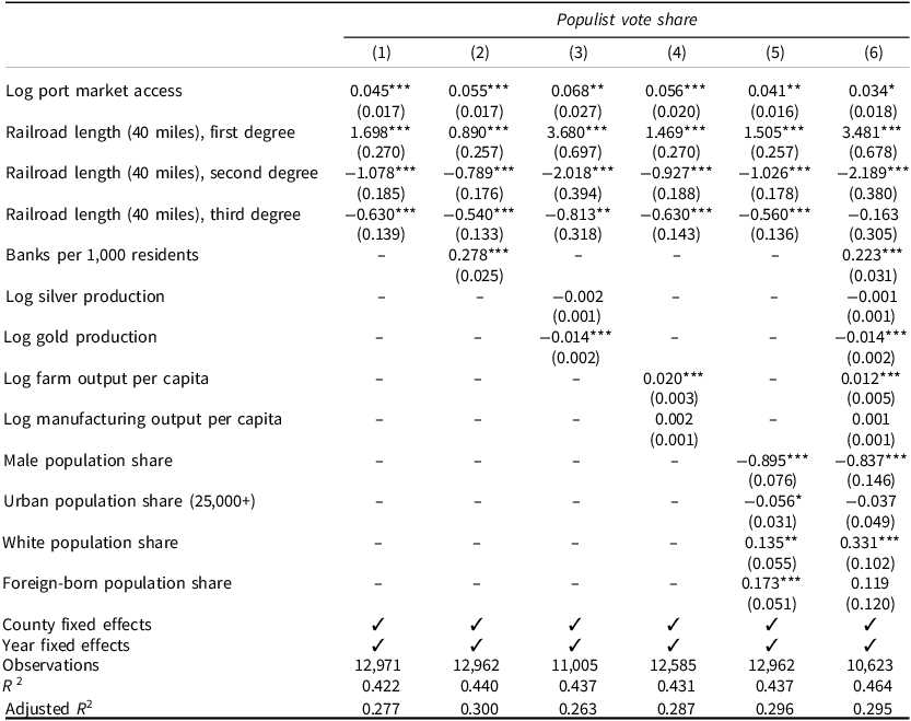
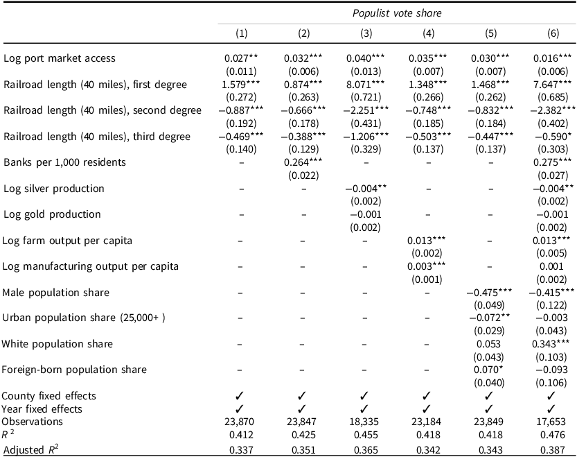
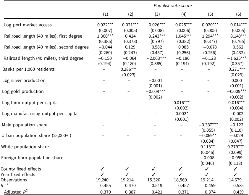
Tables 1–3 report ordinary least squares (OLS) estimates of the relationship between port market access and populist vote share across presidential, House, and gubernatorial elections. The coefficient on log port market access is consistently positive and statistically significant across specifications. A one-unit increase in log port market access is associated with an increase in populist vote share of approximately 1.4 to 6.8 percentage points, depending on the election type.
Port market access and populist vote share in presidential elections, 1870–1900

Note: all models include county and year fixed effects. Standard errors clustered at the county level are reported in parentheses. The populist party is narrowly defined. See Appendix D for regression results using the broader definition. *p < 0.1; **p < 0.05; ***p < 0.01.
Port market access and populist vote share in house elections, 1870–1900

Note: all models include county and year fixed effects. Standard errors clustered at the county level are reported in parentheses. The populist party is narrowly defined. See Appendix D for regression results using the broader definition. *p < 0.1; **p < 0.05; ***p < 0.01.
Port market access and populist vote share in gubernatorial elections, 1870–1900

Note: all models include county and year fixed effects. Standard errors clustered at the county level are reported in parentheses. The populist party is narrowly defined. See Appendix D for regression results using the broader definition. *p < 0.1; **p < 0.05; ***p < 0.01.
The estimated effects are quantitatively meaningful. In our baseline specification for presidential elections (Table 1), a one-unit increase in log port market access is associated with a 4.5 percentage-point increase in the populist vote share.
To interpret this magnitude, it is useful to consider the distribution of port market access in our sample (see Tables A.1–A.3 for summary statistics). Since the standard deviation of log port market access is 0.54, a one-standard-deviation increase is associated with a 2.4 percentage-point rise in the populist vote share. This effect size is economically significant: given the sample mean populist vote share of 8 per cent, a one-standard-deviation shock to port market access implies a 30 per cent increase relative to the baseline. Alternatively, scaling by the dispersion of the outcome, this estimate explains approximately 16 per cent of a standard deviation in populist support, suggesting that port market access is a substantial driver of voting behavior.
This effect can be interpreted as indicative of the economic, political, and social transformations that accompanied globalization. Such transformations may have included disruptions in local economies, changes in employment patterns, or perceptions of economic insecurity among certain segments of the population, particularly in agrarian regions, which populist candidates could have capitalized on.
Despite the overall positive relationship between port market access and populist voting, the coefficients tend to be larger in presidential and House elections than in gubernatorial races. One likely explanation is that federal-level contests during the nineteenth century were more directly influenced by trade policy – central to globalization – through mechanisms such as tariffs. Consequently, presidential and congressional elections, which directly affect these policies, exhibited a stronger connection with populist movements that capitalized on economic grievances related to globalization. Gubernatorial campaigns, though still affected, often centered on state-specific issues and consequently exhibited smaller, though still significant, coefficients.Footnote 5
Robustness Check
We assess the robustness of our results using several alternative specifications. First, we expand our definition of populist vote share to include a broader set of parties. As shown in Appendix D, the main findings remain unchanged: the estimated coefficients are similar in magnitude and significance to those reported in Tables 1–3.
Secondly, we address potential spatial and temporal correlation in the error terms by reporting estimates with Conley standard errors. The temporal cut-off is set to thirty years, corresponding to the maximum lag between observations in our panel. The spatial cut-off is 100 km, such that the error for a county-year observation is allowed to be correlated with those of all counties within a 100-kilometer radius in the same year, while also accounting for serial correlation within each county over time. The results, reported in Tables E.1–E.3, remain statistically significant under this adjustment.
Thirdly, we conduct placebo tests by substituting the populist vote share with Democratic and Republican vote shares from the same elections. If the relationship between market access and populist vote share is not spurious, the placebo outcomes should not show consistent patterns. Indeed, the results show no stable signs or statistical significance (see Appendix F), reinforcing our confidence that unobserved confounders or model misspecification do not drive our main findings.
Fourthly, we assess the robustness of our findings to potential omitted variable bias using two sensitivity analysis frameworks. The first is developed by Cinelli and Hazlett (Reference Cinelli and Hazlett2020). We use the sixth model in Tables 1–3 as our baseline. Contour plots in Appendix G present our results. In Figures G.1–G.3, the horizontal and vertical axes represent the partial R 2 of a hypothetical confounder with the treatment (port market access) and the outcome (populist vote share), respectively.
To contextualize the strength of potential unobserved confounders, we use the share of the white population as a benchmark, as it is one of the strongest predictors in our model. We use Figure G.1 to interpret the sensitivity analysis results. The black triangle in the bottom-left corner represents the original estimated effect size (0.034) from Table 1. The red diamonds indicate how this estimate would change if an unobserved confounder were introduced at varying multiples of the benchmark’s strength.
Our results are highly robust. As shown in Figure G.1, an unobserved confounder would need to be more than twelve times as strong as the share of the white population to nullify the effect of port market access in presidential elections. Similarly, the confounder would need to be six times as strong for House elections and nine times as strong for gubernatorial elections to explain away the estimated effects. Given the predictive power of the benchmark variable, the existence of such overwhelming unobserved confounders is unlikely.
The second approach follows Oster (Reference Oster2019), which assesses how strong selection on unobserved factors would need to be – relative to selection on observed covariates – to fully eliminate the estimated effect. We follow common practice and set the maximum attainable explanatory power to R max = 1.3 × R 2.
We implement this analysis using the full specification (Model 6 in Tables 1–3). To illustrate, we focus on the estimate for port market access in presidential elections, for which the coefficient estimate is 0.034.
Two findings suggest that this estimate is robust to omitted variable bias (see Tables G.1–G.3). First, under the assumption of equal selection on observables and unobservables (δ = 1), the implied bias-adjusted coefficient is 0.062, which is larger than the estimate reported in Column 6 of Table 1. This result implies that, under proportional selection, accounting for unobserved confounding would not attenuate the estimated relationship towards zero.
Secondly, the value of the proportionality parameter required to reduce the coefficient to zero is δ = −1.30. A negative value indicates that selection on unobservables would need to be not only strong but also opposite in sign to the selection captured by the observed controls in order to fully explain away the estimate.
Replicating this sensitivity analysis for House and gubernatorial elections generates similar conclusions. These sensitivity analyses do not demonstrate the absence of omitted variable bias. Instead, they provide a transparent assessment of the magnitude and direction of unobserved confounding required to overturn the results. Both exercises indicate that omitted variables would need to be substantially stronger than the main observed covariates – and in some cases operate in the opposite direction – to fully explain away the estimated relationship between port market access and populist electoral support.
Fifthly, we address concerns related to the entry strategy of populist parties. Our main analysis assumes that, due to limited organizational capacity, populist parties selectively entered counties more exposed to globalization shocks or competed only in selected election years. We restrict the sample to counties where at least one populist vote was recorded, yielding an unbalanced panel. However, it is plausible that populist parties intended to compete broadly, regardless of observed vote shares. To account for this possibility, we construct a balanced panel that includes all counties in all years, assigning zero vote share in cases of previously missing data. The results, presented in Appendix H, show that the positive association between market access and populist vote share remains robust and statistically significant across presidential, House, and gubernatorial elections.
Mechanism
Our central argument is that improved access to global markets exposed US farmers in the late nineteenth century to intensified international competition. As counties became more integrated into global trade networks, local producers faced price shocks originating from global supply fluctuations, and declining ability to influence pricing through product differentiation.
This exposure had two main effects. First, it amplified downside risk. A surplus harvest abroad could depress world prices, reducing returns even in high-yield years. Secondly, it increased commodification. With crops traded in large, standardized volumes, quality premiums diminished and price competition intensified. Farmers in higher-cost regions struggled to match global competitors, leading to erosion in profitability.
To evaluate these channels, we examine the relationship between port market access and county-level changes in agricultural price levels. Following Eichengreen et al. (Reference Eichengreen, Haines, Jaremski, Leblang, Hanes and Wolcott2019), we construct a fixed-basket price index tracking eleven major field crops: barley, buckwheat, corn, cotton, hay, oats, potatoes, rye, sweet potatoes, tobacco, and wheat. Crop prices are drawn from the USDA’s Crop Production Historical Track Records (USDA 2023), Carter et al. (Reference Carter, Gartner, Haines, Olmstead, Sutch and Wright2006)’s Historical Statistics of the United States, and the Census Bureau’s Historical Statistics of the United States.
Figure 8 plots annual prices for cotton, wheat, and tobacco – three major export crops – between 1870 and 1900. Prices declined substantially after the 1870s and exhibited persistent volatility through the 1890s. Appendix I presents analogous series for the remaining crops.
Prices of cotton, wheat, and tobacco in the United States, 1870–1900.

To measure the exposure of local agricultural revenues to price movements, we construct a county-level crop portfolio price index that aggregates crop-specific price changes using within-county value shares. The index captures changes in nominal agricultural revenue induced by price fluctuations, holding quantities fixed.
Let i index crops, c counties, t years, and d decennial agricultural census years. For each census year, we compute the value of crop i in county c as P i, d × Q i, c, d , where P denotes crop prices and Q denotes production. We then define crop weights as the share of each crop’s value in total county-level crop value:
 $$s_{i,c,d} = {P_{i,d}\times Q_{i,c,d}}{\sum_{j} P_{j,d}\times Q_{j,c,d}}$$
where the summation in the denominator runs over all crops produced in county c. By construction, these weights sum to one within each county and reflect local crop specialization. This value-based weighting approach ensures that the index captures each crop’s economic importance to local agricultural revenues while avoiding confounding price exposure with the absolute scale of production.Footnote 6
Using these value shares, we construct a fixed-basket price index that aggregates crop-specific price changes:
 $${\rm Change\;in\;Price\;of\;Crop\;Portfolio}_{c,t}=\sum _{i}s_{i,c,d} \Delta {\rm ln}P_{i,t}$$
where ΔlnP i, t denotes the log change in crop i’s price between t − 4 and t − 1. We use log changes because they approximate percentage changes and are symmetric with respect to price increases and decreases. The three-year lag structure is determined by data availability: the earliest available prices are from 1866. It also captures medium-term price trends rather than transitory shocks. The index is updated at each decennial census to allow for slow-moving changes in county crop composition while maintaining comparability across time.
A positive value of the index indicates an increase in nominal agricultural revenue due to rising prices, while a negative value indicates revenue losses. By construction, a 1 per cent increase in the index corresponds to a 1 per cent increase in total nominal crop revenue in the county, holding output fixed.
We estimate the following equation:
 $${\rm{Change}}\;{\rm{in}}\;{\rm{Price}}\;{\rm{of}}\;{\rm{Crop}}\;{\rm{Portfoli}}{{\rm{o}}_{c,t}} = {\beta _0} + {\beta _1}{\rm{ln}}({\rm{Port}}\;{\rm{M}}{{\rm{A}}_{{\rm{c}},{\rm{t}}}}) + {\alpha _c} + {\alpha _t} + {\epsilon_{c,t}}$$
where c indexes counties, t indexes years, α c and α t are county and year fixed effects. This model aims to isolate the effect of port market access on crop prices by controlling for unobserved heterogeneity across counties and over time. Standard errors are clustered at the county level.
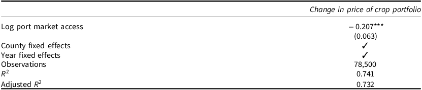
Table 4 shows a negative and statistically significant relationship between port market access and changes in crop portfolio prices. This result is consistent with our central mechanism: improved access to global markets, while expanding sales opportunities, simultaneously exposed local farmers to intensified international competition and downward price pressures. As counties became more integrated into global trade networks, local producers faced commodity prices increasingly determined by worldwide supply and demand conditions rather than local market dynamics. The resulting price declines eroded agricultural revenues even when production volumes remained stable, creating economic grievances that populist movements could mobilize.
Port market access and change in price of crop portfolio, 1870–1900

Note: standard errors clustered at the county level are reported in parentheses.
While these portfolio results clearly demonstrate that port market access led to declining crop prices, they do not by themselves distinguish between two competing interpretations. First, farmers may have experienced exogenous exposure to adverse price movements in their existing crops (the mechanism we propose). Secondly, farmers may have endogenously reallocated production towards crops that happened to experience price declines during this period (a strategic response rather than exogenous exposure). If the second interpretation were correct, the observed price declines would partly reflect farmers’ choices rather than purely exogenous shocks.
To distinguish between these interpretations, we conduct a heterogeneity analysis based on predetermined crop specialization. The logic is straightforward: if our mechanism operates through unavoidable price exposure, then counties already specialized in crops experiencing large price declines should exhibit stronger populist responses to port market access. In contrast, if the results were driven primarily by endogenous crop reallocation, we would not expect baseline (pre-period) crop composition to predict heterogeneous treatment effects.
To address this concern, we exploit cross-crop variation in national price dynamics together with heterogeneity in counties’ pre-period crop specialization. Using national crop price series, we first identify the three crops experiencing the largest price declines over the period 1870–1900: cotton (declining 72.5 per cent), barley (declining 54.5 per cent), and wheat (declining 43.5 per cent). These crops experienced systematically worse price performance than other major crops in our sample.
We then measure each county’s baseline exposure to these vulnerable crops using the value-share weights defined in Equation (4). Specifically, for the baseline census year (1870), we compute:
 $${\rm Exposure\;Decline}_c = \sum _{i\;\in \;{\rm (cotton,\;barley,\;wheat)}} s_{i,c,1870}$$
This measure captures the share of county c’s agricultural revenue derived from crops that would subsequently experience large price declines. Crucially, because this exposure measure is fixed at the baseline period (1870) – before the main expansion of port market access and populist mobilization – it captures predetermined vulnerability to adverse price movements rather than endogenous crop switching in response to market integration. Counties with high exposure decline values were already committed to producing vulnerable crops when global market integration accelerated.
We incorporate this measure into the main specification by interacting baseline exposure with port market access. Formally, we estimate:
 $$\eqalign{{\rm{PopulistShar}}{{\rm{e}}_{c,t}}{\rm{ }}& = {\beta _0} + {\beta _1}\ln ({\rm{Port}}\;{\rm{M}}{{\rm{A}}_{c,t}}) \cr& + {\beta _2}[\ln ({\rm{Port}}\;{\rm{M}}{{\rm{A}}_{c,t}}) \times {\rm{Exposure}}\;{\rm{Declin}}{{\rm{e}}_c}] + {\alpha _c} + {\alpha _t} + {\epsilon_{c,t}}}$$
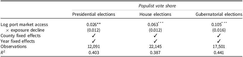
The coefficient of interest is β 2, which captures whether the port market access effect varies with predetermined crop exposure. Table 5 presents the results across three types of elections (presidential, House, and gubernatorial). In all three specifications, β 2 is positive and statistically significant, indicating that the effect of port market access on populist voting is substantially larger in counties that were initially more specialized in crops experiencing large national price declines.
Port market access, price declines, and populist voting, 1870–1900

Note: standard errors clustered at the county level are reported in parentheses.
This heterogeneity pattern provides strong evidence for our price-based exposure mechanism. Counties that were ex ante more vulnerable to adverse price movements – as measured by their 1870 crop composition – experienced disproportionately strong political backlash when port market access improved. The results indicate that farmers who were already committed to producing vulnerable crops – and thus unable to switch easily to alternative crops – bore the brunt of globalization shocks and responded by supporting populist movements. This interpretation is consistent with historical accounts emphasizing that many farmers, particularly cotton producers in the South and wheat producers in the Great Plains, faced substantial switching costs due to soil conditions, climate constraints, specialized equipment, and credit arrangements tied to specific crops.
Conclusion
In this paper, we explore how globalization led to the rise of electoral populism in the United States from 1870 to 1900. Our findings reveal a significant and positive relationship between globalization – measured through port market access – and support for populist parties in elections at every level.
Utilizing a unique dataset, we tracked the evolution of American electoral populism and documented fluctuations in party vote shares and political orientations. This period coincided with significant advancements in transportation technologies, such as railroads and steamships. These technologies dramatically lowered transportation costs and further integrated global markets. Not only did these developments catalyze the flow of goods, but they also intensified the transmission of economic shocks and price volatility.
Our results indicate that the rise of populism was closely tied to economic grievances that were exacerbated by globalization. Our empirical strategy explored how increased port market access affected local economies. We discovered that as farmers’ integration into global markets deepened, they encountered heightened competition and price instability from global markets. This exposure led to economic disenfranchisement among farmers, who, facing declining agricultural incomes and unable to influence global commodity prices, found themselves increasingly marginalized. This economic distress provided fertile ground for populist rhetoric, which resonated strongly with those adversely affected by international trade.
While we have provided robust evidence on how the first wave of globalization contributed to the rise of electoral populism in the United States, we would like to explain why populist parties declined after William Jennings Bryan’s loss, even as globalization expanded. The answer lies in the resilience of populist doctrines, despite the organizational collapse of the party itself (Hicks Reference Hicks1931). During the early twentieth century, many populist demands were adopted and transformed by both the Democratic and Republican parties (Postel Reference Postel2007).
For example, populists had demanded that the federal government construct warehouses, or subtreasuries, to store crops at harvest. The Warehouse Act of 1916 marked significant progress towards fulfilling these demands by enabling the US Department of Agriculture to license warehousemen and authorize them to ‘receive, weigh, and grade farm products’. Moreover, it allowed owners to borrow money using warehouse receipts as collateral. Additionally, populist platforms usually called for borrowing money at a low rate of interest. Through the establishment of Farm Loan Banks by an act of 1916 and the Federal Intermediate Credit Banks by an act of 1923, the government not only established a comprehensive system of rural credits to meet farmers’ needs but also facilitated their access to loans on favorable terms, ranging from six months to three years. Thus, while the original populist party waned, its core ideas found new expression and were instrumental in shaping early twentieth-century American policies (Hicks Reference Hicks1931).
Our study not only enriches the existing literature on globalization and populism but also positions these discussions within a historical context. Extensive research affirms that globalization helps to fuel the rise of present-day populist movements. However, our findings demonstrate that this relationship has deep historical roots dating back to the second half of nineteenth-century America. By detailing the conditions under which populism thrived in response to the first wave of globalization, this paper underscores the cyclical nature of these phenomena and highlights the recurring socio-economic catalysts behind political discontent.
Overall, our analysis reveals that the socio-economic disruptions caused by globalization, such as market integration and increased exposure to global economic fluctuations, have consistently served as fertile ground for populist sentiments. This historical perspective is crucial for understanding the persistence of populism as a political strategy in times of economic uncertainty (Han et al. Reference Han, Milner and Mitchener2023). It illustrates that the appeal of populism often arises from its ability to articulate widespread grievances and position itself as an alternative to the perceived failures of traditional political elites, a scenario that is evident both in the past and present.
While our study documents a robust reduced-form relationship between port market access and populist voting, it does not claim that port market access provides a fully exogenous source of variation. Transportation networks, port development, and regional economic trajectories were jointly shaped by long-run political and economic forces. While our design mitigates these concerns using county fixed effects, many controls, and sensitivity analyses, future research could further strengthen identification by exploiting plausibly exogenous variation in trade connectivity – such as natural harbor characteristics, historical shipping routes, or technological shocks to maritime transport that differentially affected ports over time. Such approaches would help disentangle the causal impact of globalization from broader processes of regional development.
A second limitation concerns the interpretation of port market access as a measure of globalization rather than domestic market integration. Major ports were also large urban consumption centers, and access to ports may have increased counties’ exposure to both international and domestic demand. While our measure is weighted by international trade volumes and restricted to port counties to sharpen its globalization content, future work could further decompose international and domestic channels – for example, by constructing parallel measures of access to non-port urban markets or by exploiting variation in export versus import intensity across ports. Such extensions would clarify the extent to which the populist backlash reflected exposure to global competition specifically, as opposed to broader integration into national markets.
Supplementary material
The supplementary material for this article can be found at https://doi.org/10.1017/S0007123426101537.
Data availability statement
Replication data for this article can be found in Harvard Dataverse at: https://doi.org/10.7910/DVN/RDQWTY.
Acknowledgments
We are grateful to Anne Hartingh and Rick Hornbeck for generously sharing their data. We also extend our appreciation for the valuable comments and suggestions from Quan Li, Ken Scheve, Theo Serlin, and the participants at the 2024 APSA, 2024 IPES, and 2025 ISA. We thank Nitheesha Nakka for assistance with replication.
Financial support
This research received no specific grant from any funding agency, commercial or not-for-profit sectors.
Competing interests
None.


 Open access