


1. Introduction
The early design phase has great influence on the development process of new products (Reference Ehrlenspiel and MeerkammEhrlenspiel & Meerkamm, 2017). This conceptual phase not only provides the ground for the design process itself, it also has a major impact on the finalized product (Reference Bender and GerickeBender & Gericke, 2021; Verein Deutscher Ingenieure, 2019). Functional decomposition and the consequent Function Structure are central in this stage of the design process. The overall function of a new product is derived from its requirements. By decomposing this overall function into base functions and their connections, the purpose of the product becomes accessible for further steps in the design process (Reference RothRoth, 2000). The resulting structure clarifies the flows of materials, energy and information through the product. The focus here is a static specification for the conceptual design phase, rather than a dynamic behaviour model.
However, most of the Roth-style structures only provide information about the routing of the three entities between functions and not their magnitudes and units. This leaves design engineers with significant uncertainty, since they cannot check on conservation laws, detect infeasibilities or compare competing Function Structures on measurable grounds.
The decomposition process is a tedious and complex task, usually depending on the experience of specialized design engineers. At the same time, it is susceptible to inconsistencies at the interfaces between functions.
Nevertheless, recent research by Reference Rosenthal, Demke, Mantwill and NiggemannRosenthal et al. (2024) and Reference Haddad and SeibelHaddad and Seibel (2025) has shown that decomposition can be automated using Artificial Intelligence (AI) planning and Large Language Model (LLM) assisted approaches. These approaches operate on qualitative graphs, ensuring logical connectivity, but they cannot check unit consistency or conservation.
Formal-methods results show that properties of symbolic system models can be verified from formal, solver-ready specifications (Reference Cimatti, Griggio, Mover, Roveri and TonettaCimatti et al., 2022). At the same time, emerging automation for functional modelling already produces such machine-readable models in the conceptual design phase. Yet, quantitative consistency checks are still missing. This combination motivates a problem framing that also carries quantitative aspects and consistency criteria into the conceptual design phase.
The resulting challenge consists of three deficits. First, a problem framing deficit: An extended problem formalization is needed, which enables quantitative checks without giving up abstraction advantages of the early design phase. Second, a representation deficit: Functions and their structures need to be represented in a different way in order to cater to quantitative measures and conservation laws. The final deficit is an algorithmic one. Automated functional decomposition must still be possible by AI algorithms, when including quantitative measures.
This challenge can be referred to as the Quantitative Functional Decomposition Problem (QFDP), the task of deriving a working Function Structure that, in addition to logical consistency, makes quantitative consistency checkable in conceptual design phase. For practitioners this means earlier plausibility of concepts with units and ranges and clearer requirements for downstream work.
This leads to the following research questions (RQ).
RQ 1: How should the QFDP be formalized to incorporate quantitative consistency and make it accessible to AI algorithms?
RQ 2: How does extending the functional decomposition from qualitative to quantitative measures change the representation and composition of functions and their structures?
RQ 3: Which algorithmic approach is suited to find correct solutions for a given QFDP?
This work introduces the Quantitative Function Structurer (QFS). This new algorithm is able to find meaningful quantified solutions for a given QFDP. A formalized framework supports the approach by defining the problem and making it processable for symbolic AI algorithms. The QFS is evaluated in two real world case studies by assessing its correctness in building quantified solutions for the problems.
2. Related work
The VDI 2222-1 (1997) defined functions as relations between input entities, output entities and their internal mapping. The emphasis is on abstract and solution neutral formulations to avoid specific assignments and ensure comparability. Pahl and Beitz (Reference Bender and GerickeBender & Gericke, 2021) identify Function Structures as the central working artefact in the conceptual design phase. Resulting from the requirements, the overall function gets systematically decomposed into subfunctions and their relations. The VDI 2221-1 (2019) embeds the Function Structure in the development process in the same way and gives the procedure a methodical foundation. These references set the standard. However, they focus primarily on qualitative aspects and omit explicit unit and dimension checks and quantitative measures. In addition, VDI/VDE 3682 (2005) formalizes process descriptions in terms of states and process operators, which is conceptually close to functional modelling. Yet, it likewise remains qualitative and does not enforce unit consistency.
Reference RothRoth (2000; 2001) introduced a general set of 30 functions for the three entities material, energy and information. He provides a uniform vocabulary for the functional decomposition in the early design phase. These Roth Functions enable the systematic and consistent modelling of Function Structures, but they do not prescribe magnitudes, units or parameterized interfaces.
Reference Koller and KastrupKoller and Kastrup (1998) anchor functions in an engineering methodology emphasizing the cause-and-effect relationship as the foundation of technical functions. This supports the systematic decomposition, yet this approach remains qualitative and omits any quantitative structure.
Reference GeroGero (1990) describes functions as the link between purpose description i.e. requirements and the actual physical behaviour. He thereby emphasises the role of the function concept for decisions in the early stages of the development process, focusing on conceptual clarity rather than quantitative consistency.
Over time different approaches have been elaborated in order to automate and systematize the process of modelling a Function Structure in the early design phase.
Notably, the function-behavior-state (FBS) modeler proposed by Reference Umeda, Ishii, Yoshioka, Shimomura and TomiyamaUmeda et al. (1996) is a knowledge-based tool and shows an early example of computer supported functional modelling. However, functional decomposition remains largely expert driven and qualitative with no unit and dimension enforcement.
Reference Kitamura and MizoguchiKitamura and Mizoguchi (2003) present an ontology-based systematization of function knowledge. They separate functions, i.e. what must be achieved, with ways, i.e. how it is achieved. While organizing functions, their approach does not automatically decompose the overall product function into a structure.
Reference Tensa, Edmonds, Ferrero, Mikes, Soria Zurita, Stone and DuPontTensa et al. (2019) use association rules in design repositories to extract component-function-flow associations. The data driven approach relies on existing data to derive functional chains and partial structures, supporting the decomposition process but without taking quantifiability into account. Complementing this strand, Reference Mikes, Edmonds, Stone and DuPontMikes et al. (2021) introduce AutoFunc as a practical tool for semi-automated generation and verification of functional models from repositories. Their approach addresses consistency and reuse. However, it remains primarily qualitative and does not perform quantitative consistency checks.
Reference Mohammed and ShammariMohammed and Shammari (2021) propose a rule-based procedural algorithm to construct Function Structures. They explicitly address the derivation of these structures from customer requirements. While their approach pays attention to consistency and physical correctness it also does only take qualitative measures into account and is limited to its reconciled functional basis.
Reference Rosenthal, Demke, Mantwill and NiggemannRosenthal et al. (2024) have shown that the problem of finding a working Function Structure can be expressed as a planning problem. In this formulation, Roth Functions are modelled as actions and a partial-order planner (POP) is used to derive a structure from specified boundary conditions. The authors demonstrate their approach by using POP to solve decomposition problems, but the representation remains qualitative and it cannot enforce units/conservation or compute feasible quantitative interfaces.
Reference Haddad and SeibelHaddad and Seibel (2025) propose to frame the decomposition problem as a knowledge-graph construction. They make use of an LLM and further improve the results with a Monte Carlo tree search (MCTS) loop. While this approach shows improvements over the plain usage of LLMs, the authors still report substantial structural errors and the need for expert review. In addition, the representation remains qualitative.
Across standards, textbooks and foundational work, Function Structures are established as a central solution neutral artefact. Yet, they are qualitative. Model-based, rule-based, data-driven, planning-based and LLM-based approaches demonstrate that functional decomposition can be supported and automated but likewise operate on qualitative graphs without explicit unit and dimension consistency or conservation checks.
3. Solution
The previous section pointed out that existing approaches rely on qualitative measures to ensure logical correctness within the Function Structure only, entirely neglecting any kind of quantity. Inspired by the approach of Reference Rosenthal, Demke, Mantwill and NiggemannRosenthal et al. (2024), this paper aim to extend automated decomposition to quantifiable Function Structures. Therefore, the initial problem formalization needs to be adapted and extended.
3.1. Formalization
Definition 1 Index Sets (finite domains): ${{\it \Phi}} = \left\{ {solid,liquid,gas} \right\}$ $E = \left\{ {chemical,electrical,kinetic,potential,thermal} \right\}$ $I = \left\{ {analog,digital,quantum} \right\}$ ${U_M}{\rm{\;}}a{\rm{\;}}countable{\rm{\;}}universe{\rm{\;}}of{\rm{\;}}material{\rm{\;}}identifiers$ $M \subseteq {U_M}{\rm{\;}}a{\rm{\;}}finite{\rm{\;}}material{\rm{\;}}set{\rm{\;}}for{\rm{\;}}a{\rm{\;}}given{\rm{\;}}problem$ $S = \left\{ {MFlow,EFlow,IFlow} \right\}$ ${U_P}{\rm{\;}}a{\rm{\;}}countable{\rm{\;}}universe{\rm{\;}}of\;Properties$ $P \subseteq {U_P}{\rm{\;}}a{\rm{\;}}finite{\rm{\;}}Property{\rm{\;}}set{\rm{\;}}for{\rm{\;}}a{\rm{\;}}given{\rm{\;}}problem$
Definition 2 Problem spaces: $Material{\rm{\;}}space\!:{V_{mat}}\left( M \right) = \{ {x_M}|{x_{M}}:M \times {\it \Phi} \to \mathbb{R}\} $ $Energy{\rm{\;}}space\!:{V_{en}} = \{ {x_E}|{x_E}:E \to \mathbb{R}\} $ $Information{\rm{\;}}space\!:{V_{info}} = \{ {x_I}|{x_I}:I \to \mathbb{R}\} $ $Stream{\rm{\;}}space\!:{V_{stream}} = \{ {x_S}|{x_S}:S \to \mathbb{R}\} $ $Property{\rm{\;}}space\!:{V_{prop}} = \{ {x_P}|{x_P}:P \to \mathbb{R}\} $
Definition 3 Entity space for a given problem: $V=V_{mat} \bigoplus V_{en} \bigoplus V_{info} \bigoplus V_{stream} \bigoplus V_{prop}$
 $$\dim V = \left| {\it \Phi} \right| \cdot \left| M \right| + \left| E \right| + \left| I \right| + \left| S \right| + \left| P \right| = 3 \cdot \left| M \right| + 5 + 3 + 3 + \left| P \right|$$
Definition 4 Entity vector (state of one entity):
Each entity is uniquely defined by a vector
 $$x \in V$$
, assigning specific values to all components of
$$x \in V$$
, assigning specific values to all components of
 $$V$$
, with
$$V$$
, with
 $$x = \left( {{x_M},{x_E},{x_I},{x_S},{x_P}} \right){\rm{\;and\;}}{x_M}:{\rm{\;}}M \times {\it \Phi} \to \mathbb{R},{x_E}:{\rm{\;}}E \to \mathbb{R},{x_I}:{\rm{\;}}I \to \mathbb{R},{x_S}:{\rm{\;}}S \to \mathbb{R},{x_P}:{\rm{\;}}P \to \mathbb{R}$$
.
$$x = \left( {{x_M},{x_E},{x_I},{x_S},{x_P}} \right){\rm{\;and\;}}{x_M}:{\rm{\;}}M \times {\it \Phi} \to \mathbb{R},{x_E}:{\rm{\;}}E \to \mathbb{R},{x_I}:{\rm{\;}}I \to \mathbb{R},{x_S}:{\rm{\;}}S \to \mathbb{R},{x_P}:{\rm{\;}}P \to \mathbb{R}$$
.
Definition 5 A control parameter
 $$c \in \mathbb{R}$$
is a scalar.
$$c \in \mathbb{R}$$
is a scalar.
Definition 6 A Roth Function
 $$f \in R$$
is a tuple:
$$f \in R$$
is a tuple:
 $$f = ( {{n_f},{i_f},{o_f},{c_f}} )$$
, where
$$f = ( {{n_f},{i_f},{o_f},{c_f}} )$$
, where
 $${n_f}$$
is a unique name for the function,
$${n_f}$$
is a unique name for the function,
 $${i_f},{o_f}$$
with
$${i_f},{o_f}$$
with
 $${i_f},{o_f} \in V$$
are inputs and outputs of the function and
$${i_f},{o_f} \in V$$
are inputs and outputs of the function and
 $${c_f}$$
is a control parameter specifying the quantitative transition from
$${c_f}$$
is a control parameter specifying the quantitative transition from
 $${i_f}$$
to
$${i_f}$$
to
 $${o_f}$$
.
$${o_f}$$
.
Definition 7 The Roth Function Set R is the set of all Roth Functions:
 $$R = \left\{ {f{\rm{|}}f{\rm{\;}}represents{\rm{\;}}a{\rm{\;}}Roth{\rm{\;}}Function} \right\}$$
Definition 8 The Quantitative Roth Catalogue is a subset of the Roth Functions (usable subset):
 $$QRC \subseteq R$$
.
$$QRC \subseteq R$$
.
Definition 9 A Function Structure
 $$FS$$
is an admissible directed graph
$$FS$$
is an admissible directed graph
 with:
with:
 $$N$$
a finite set of nodes
$$N$$
a finite set of nodes
 $$K \subseteq N \times N$$
a set of directed edges
$$K \subseteq N \times N$$
a set of directed edges
 $${\it \Lambda} :N \to {\rm{R}}$$
a labeling, which maps each node to its Roth Function
$${\it \Lambda} :N \to {\rm{R}}$$
a labeling, which maps each node to its Roth Function
For any edge
 $$\left( {u,w} \right) \in {\rm{K}}$$
, let
$$\left( {u,w} \right) \in {\rm{K}}$$
, let
 $${\it \Lambda} \left( u \right) = \left( {{n_u},{i_u},{o_u},{c_u}} \right){\rm{\;}}$$
and
$${\it \Lambda} \left( u \right) = \left( {{n_u},{i_u},{o_u},{c_u}} \right){\rm{\;}}$$
and
 $${\it \Lambda} \left( w \right) = \left( {{n_w},{i_w},{o_w},{c_w}} \right)$$
. Then the edge is admissible iff
$${\it \Lambda} \left( w \right) = \left( {{n_w},{i_w},{o_w},{c_w}} \right)$$
. Then the edge is admissible iff
 $${o_u}$$
is compatible with
$${o_u}$$
is compatible with
 $${i_w}$$
under the combination rules associated with the Roth Functions.
$${i_w}$$
under the combination rules associated with the Roth Functions.
Definition 10 A Quantitative Functional Decomposition Problem
 $$QFDP$$
is a tuple:
$$QFDP$$
is a tuple:
 $$QFDP = \left( {{S_x},{i_x},{o_x},{\rm{Q}}RC} \right)$$
, where
$$QFDP = \left( {{S_x},{i_x},{o_x},{\rm{Q}}RC} \right)$$
, where
 is a finite set of entity vector states. For every
 $${s_x} \in {S_x}$$
there exists
$${s_x} \in {S_x}$$
there exists
 $$m \in {\mathbb{N}_{\! \gt \!0}}$$
with
$$m \in {\mathbb{N}_{\! \gt \!0}}$$
with
 $${s_x} = \left( {{x_1}, \ldots ,{x_m}} \right),\;{x_j} \in V,$$
for all
$${s_x} = \left( {{x_1}, \ldots ,{x_m}} \right),\;{x_j} \in V,$$
for all
 $$j = 1, \ldots ,m$$
. The input to the
$$j = 1, \ldots ,m$$
. The input to the
 $$QFDP$$
is
$$QFDP$$
is
 $${i_x}$$
and
$${i_x}$$
and
 $${o_x}$$
is the output, with
$${o_x}$$
is the output, with
 $${i_x},{o_x} \in {S_x}$$
.
$${i_x},{o_x} \in {S_x}$$
.
 $$QRC$$
is the Quantitative Roth Catalogue.
$$QRC$$
is the Quantitative Roth Catalogue.
Definition 11 The solution
 $${f_d}$$
to a
$${f_d}$$
to a
 $$QFDP$$
is a finite ordered sequence of Roth Functions
$$QFDP$$
is a finite ordered sequence of Roth Functions
 $${f_d} = \left( {{f_1}, \ldots ,{f_k}} \right),k \in {\mathbb{N}_{\! \gt \! 0}},{f_j} \in QRC,$$
for all
$${f_d} = \left( {{f_1}, \ldots ,{f_k}} \right),k \in {\mathbb{N}_{\! \gt \! 0}},{f_j} \in QRC,$$
for all
 $$j$$
, such that there exists a state
$$j$$
, such that there exists a state
 $$s^{\prime} \in {S_x}$$
with
$$s^{\prime} \in {S_x}$$
with
 $${i_x}\mathop \Rightarrow \limits^{{f_d}} s^{\prime}$$
and
$${i_x}\mathop \Rightarrow \limits^{{f_d}} s^{\prime}$$
and
 $$s^{\prime} \models {o_x}$$
, which induces the Function Structure
$$s^{\prime} \models {o_x}$$
, which induces the Function Structure
 $$FS\left( {{f_d}} \right)$$
.
$$FS\left( {{f_d}} \right)$$
.
This section is the direct answer to RQ 1. By using the formalizations, quantitative consistency can be incorporated into the Decomposition Problem and make it accessible to AI algorithms.
3.2. Roth catalogue adaptation
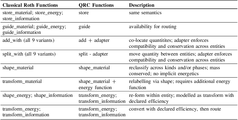
The Quantitative Roth Catalogue (QRC) from Definition 8 provides six function families, i.e. split, add, shape, transform, guide and store. These differ from the classical Roth Functions Reference Roth(Roth, 2000) only in quantitative refinement. Each QRC function declares a parent Roth Function
 $$r \in R$$
, so that
$$r \in R$$
, so that
 $$QRC \subseteq R$$
holds true by construction. More precisely, guide, add, split and store all refine their counterparts. Transform_energy/information refines transform. For shape_material, the parent is shape when only kind changes and transform_material when the phase label changes. The associated energetics are explicitly modelled in the energy domain rather than being implicit in the material operator as in the classical Roth Functions.
$$QRC \subseteq R$$
holds true by construction. More precisely, guide, add, split and store all refine their counterparts. Transform_energy/information refines transform. For shape_material, the parent is shape when only kind changes and transform_material when the phase label changes. The associated energetics are explicitly modelled in the energy domain rather than being implicit in the material operator as in the classical Roth Functions.
In this implementation, store and guide act on availability states. Store marks an entity as not available for routing, whereas guide marks it as available for routing. The add family co-locates specified quantities from two sources into a destination without creating or destroying any quantity. On the other hand, the split family moves a specified quantity from a source to a destination, likewise without creation or destruction. Cross-entity interactions for add and split are realized with interface adapters, which enforce unit compatibility, conservation of mass and energy and, where declared, coupling constraints such as stoichiometric ratios.
The shape_material function reclassifies material already present within an entity across kinds and/or phases while conserving total mass. If a phase change requires energy, e.g. melting, that energy is supplied by energy functions and routed via subsequent add or split operations. The transform family converts quantities between forms within an entity. Transform_energy and transform_information change energy or information with declared efficiencies, while material phase or form relabeling is represented with shape_material plus explicit energy transfers.
Table 1 summarizes the mapping from the initial Roth Functions to the QRC and clarifies how classical operators are realized in the quantitative setting used by the following algorithm.
RQ 2 is directly answered by describing the quantitative representation for functions and criteria, which enforce conservation and compatibility throughout the Function Structure. In that way qualitative links are replaced with parameterized and checkable interfaces.
Quantitative adaptation

3.3. Algorithm
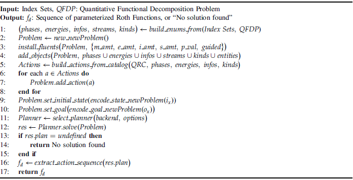
The functional decomposition is addressed by expressing it as a planning problem. Working in a numerical-planning setting where control parameters modulate the numerical effects of actions, the planning-as-satisfiability with Satisfiability Modulo Theories (SMT) is adopted as a suitable base paradigm Reference Heesch, Cimatti, Ehrhardt, Diedrich, Niggemann and Endriss(Heesch, Cimatti, et al., 2024). The planning problem is formulated using the feature-vector–based state-space representation introduced by Reference Heesch, Ehrhardt and NiggemannHeesch, Ehrhardt, and Niggemann (2024), which encodes high-dimensional states as vectors and provides a uniform interface for translating the planning problem into an SMT formula. The resulting Algorithm 1 is shown below.
Quantitative Function Structurer

The input needed for the Quantitative Function Structurer are the Index Sets from Definition 1 and the actual
 $$QFDP$$
from Definition 10. The output is either a solution to the
$$QFDP$$
from Definition 10. The output is either a solution to the
 $$QFDP$$
as in Definition 11 or an indication that no solution can be found. The algorithm starts with building the concrete domain for the instance in line 1, where the state space depends on the initial and the goal state of the
$$QFDP$$
as in Definition 11 or an indication that no solution can be found. The algorithm starts with building the concrete domain for the instance in line 1, where the state space depends on the initial and the goal state of the
 $$QFPD$$
. In line 2, a
$$QFPD$$
. In line 2, a
 $$Problem$$
is created as an empty new problem, building on the Definitions 2-4. The next line registers the fluent families on the
$$Problem$$
is created as an empty new problem, building on the Definitions 2-4. The next line registers the fluent families on the
 $$Problem$$
, realizing the components of the entity space
$$Problem$$
, realizing the components of the entity space
 $$V$$
as typed numeric state variables. Line 4 populates the object domains of the
$$V$$
as typed numeric state variables. Line 4 populates the object domains of the
 $$Problem$$
with the union of all instance sets
$$Problem$$
with the union of all instance sets
 $$\left( {phases \cup energies \cup infos \cup streams \cup kinds \cup entities} \right)$$
.
$$\left( {phases \cup energies \cup infos \cup streams \cup kinds \cup entities} \right)$$
.
The following line 5 compiles the
 $$QRC$$
into
$$QRC$$
into
 $$Actions$$
. Each Roth tuple
$$Actions$$
. Each Roth tuple
 $$f = ( {{n_f},{i_f},{o_f},{c_f}} )$$
becomes a parameterized action with preconditions and effects. The for-loop from line 6 to line 8 adds all previously built
$$f = ( {{n_f},{i_f},{o_f},{c_f}} )$$
becomes a parameterized action with preconditions and effects. The for-loop from line 6 to line 8 adds all previously built
 $$Actions$$
to the action set of the
$$Actions$$
to the action set of the
 $$Problem$$
. This makes the admissible Roth Function transitions available for planning as defined in Definition 9.
$$Problem$$
. This makes the admissible Roth Function transitions available for planning as defined in Definition 9.
Line 9 then encodes the input state
 $${i_x} \in {S_x}$$
from Definition 10 as a concrete valuation of the fluent families and installs it as a planning initial state. In the same way line 10 encodes the desired output state
$${i_x} \in {S_x}$$
from Definition 10 as a concrete valuation of the fluent families and installs it as a planning initial state. In the same way line 10 encodes the desired output state
 $${o_x} \in {S_x}$$
from Definition 10 as goal constraints over the fluent families. Then a one-shot planning backend with given options is selected in line 11. This backend yields the solver for handling the planning problem. The choice is implementation specific and independent of the formal definitions given above. In line 12 the selected solver is invoked on the constructed planning problem. The result contains a candidate plan, meaning an ordered sequence of actions, i.e. Roth Functions or will indicate a failure or timeout.
$${o_x} \in {S_x}$$
from Definition 10 as goal constraints over the fluent families. Then a one-shot planning backend with given options is selected in line 11. This backend yields the solver for handling the planning problem. The choice is implementation specific and independent of the formal definitions given above. In line 12 the selected solver is invoked on the constructed planning problem. The result contains a candidate plan, meaning an ordered sequence of actions, i.e. Roth Functions or will indicate a failure or timeout.
The if-condition from line 13 to line 15 checks for an undefined plan or unsuccessful status. If no plan is available, the algorithm returns “No solution found” immediately. On a side note, this test does not reject empty plans of length 0, since these plans are valid when
 $${i_x}$$
already satisfies
$${i_x}$$
already satisfies
 $${o_x}$$
. However, if the solver was successful, the ordered action sequence is extracted and assigned to
$${o_x}$$
. However, if the solver was successful, the ordered action sequence is extracted and assigned to
 $${f_d}$$
. The final line returns the solution which can directly be used to build the Function Structure
$${f_d}$$
. The final line returns the solution which can directly be used to build the Function Structure
 $$FS$$
.
$$FS$$
.
The shown and explained Algorithm 1 answers RQ 3.
4. Experimental results
The algorithm is assessed using a coffee maker and a Fused Deposition Modeling (FDM) printer as case studies. The experiments were conducted on a system with an AMD Ryzen 9 9950X 16-core processor and 96 GB RAM. The planning problems derived from the functional decomposition problems were encoded in the Unified Planning Framework (UPF) Reference Micheli, Bit-Monnot, Röger, Scala, Valentini, Framba, Rovetta, Trapasso, Bonassi, Gerevini, Iocchi, Ingrand, Köckemann, Patrizi, Saetti, Serina and Stock(Micheli et al., 2025) and solved using the Tempest planning engine, which is based on Reference Panjkovic and MicheliPanjkovic and Micheli (2023, Reference Panjkovic and Micheli2024).
4.1. Coffee maker
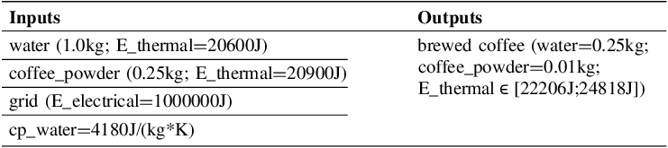
The first case study is a coffee maker. It is a suitable benchmark because it couples material and energy entities in a simple checkable way. Yet, it still exercises unit checks, conservation and interface compatibility. Its overall function is to produce hot coffee given it has access to water, coffee powder and electricity. The quantified inputs and outputs are displayed in Table 2.
Coffee maker inputs and outputs

Presenting the problem to the Quantitative Function Structurer using the UPF and the Tempest planning engine, it outputs the following solution: $\{ {add\_material\;( {src1 = water,\;src2 = coffee\_powder,\;dst = brewed\_coffee,\;amount1 = 1/4,\;amount2 = 5764607523034235/576460752303423488 \approx 0.01} )} \}$
;
$\{ {add\_material\;( {src1 = water,\;src2 = coffee\_powder,\;dst = brewed\_coffee,\;amount1 = 1/4,\;amount2 = 5764607523034235/576460752303423488 \approx 0.01} )} \}$
; $\{ {guide\_entity( {x = grid} )} \}$
;
$\{ {guide\_entity( {x = grid} )} \}$
;
 $$\{ {transform\_energy\_electrical\_to\_thermal( {x = grid,\;E\_in = 1000000} )} \}$$
;
$$\{ {transform\_energy\_electrical\_to\_thermal( {x = grid,\;E\_in = 1000000} )} \}$$
;
 $$\{ {guide\_entity ( {x = water} )} \}$$
;
$$\{ {guide\_entity ( {x = water} )} \}$$
;
 $$\{ {split\_energy\_thermal( {src = grid,\;dst = brewed\_coffee,\;E\_in = 24818} )} \}$$
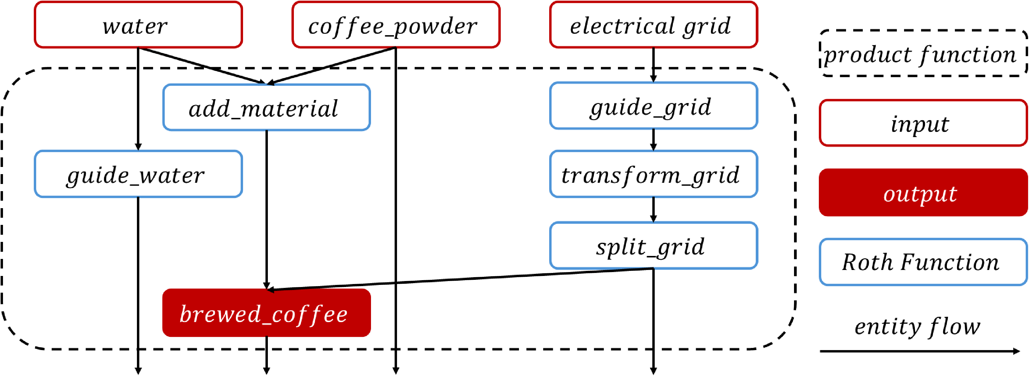
The resulting Function Structure is depicted in Figure 1 shown below.
Derived function structure for the coffee maker

First, the desired masses of water and coffee powder are added together. Then the electricity is guided, before the entire electrical energy is transformed into thermal energy. The next sub function is the guidance of what is left of the water, followed by loading the brewed coffee with the appropriate amount of thermal energy. The final state entails the desired output of the brewed coffee along with the rest of the water, coffee powder and thermal energy.
4.2. FDM printer
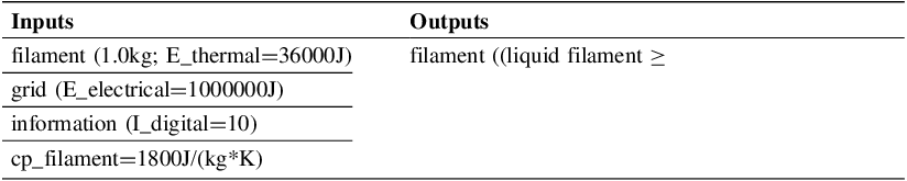
The second case study is a minimal FDM printer. It complements the coffee maker as a suitable benchmark because it exercises also information alongside material and energy in one coherent instance. In contrast to the coffee maker, it also requires a material phase change. It thereby further stresses unit checks, conservation and interface compatibility across the entities. The overall function is to produce a two phased filament loaded with information. The quantified inputs and outputs are listed in Table 3.
FDM printer inputs and outputs

Inputting the QFDP containing the above inputs and outputs in the Quantitative Function Structurer returns the following solution:
 ;
;
 $$\{ {Transform\_information\_digital\_to\_analog( {x = information,\;I\_in = 5761004643332338483/576460752303423488 \approx 10.00})} \}$$
;
$$\{ {Transform\_information\_digital\_to\_analog( {x = information,\;I\_in = 5761004643332338483/576460752303423488 \approx 10.00})} \}$$
;
 $$\{ {Guide\_entity( {x = grid} )} \}$$
;
$$\{ {Guide\_entity( {x = grid} )} \}$$
;
 $$\{ {Split\_energy\_electrical( {src = grid,\;dst = filament1,\;E\_in = 292733975779082240000/4278419646001971 \approx 68421.05})} \}$$
;
$$\{ {Split\_energy\_electrical( {src = grid,\;dst = filament1,\;E\_in = 292733975779082240000/4278419646001971 \approx 68421.05})} \}$$
;
 $$\{ {Transform\_information\_digital\_to\_analog( {x = information,\;I\_in = 3602879701896397/576460752303423488 \approx 0.01})} \}$$
;
$$\{ {Transform\_information\_digital\_to\_analog( {x = information,\;I\_in = 3602879701896397/576460752303423488 \approx 0.01})} \}$$
;
 $$\{ {Shape\_material\_filament\_to\_filament1\_liquid( {x = filament,\;amount = 900719925474099/4503599627370496 \approx 0.20})} \}$$
;
$$\{ {Shape\_material\_filament\_to\_filament1\_liquid( {x = filament,\;amount = 900719925474099/4503599627370496 \approx 0.20})} \}$$
;
 $$\{ {Guide\_entity( {x = information} )} \}$$
;
$$\{ {Guide\_entity( {x = information} )} \}$$
;
 $$\{ {Split\_information\_analog( {src = information,\;dst = filament,\;I\_in = 10} )} \}$$
;
$$\{ {Split\_information\_analog( {src = information,\;dst = filament,\;I\_in = 10} )} \}$$
;
 $$\{ {Transform\_energy\_electrical\_to\_thermal( {x = filament1,\;E\_in = 292733975779082240000/4278419646001971 \approx 68421.05})} \}$$
;
$$\{ {Transform\_energy\_electrical\_to\_thermal( {x = filament1,\;E\_in = 292733975779082240000/4278419646001971 \approx 68421.05})} \}$$
;
 $$\{ {Add\_material\_filament\_liquid\_filament1\_liquid( {src1 = filament,\;src2 = filament,\;dst = filament1,\;amount1 = 3602879701896397/4503599627370496 \approx 0.80,\;amount2 = 900719925474099/4503599627370496 \approx 0.20})} \}$$
The resulting Function Structure is shown in Figure 2.
Derived function ftructure for the FDM printer

The filament is first transformed into a liquid state. Afterwards, the digital information is getting transformed into analog information. In a third step the electricity is being guided right before a part of it is being split off for usage in a, at this point empty, filament entity. The next function is to again transform an amount of information from digital to analog. Then, the appropriate amount of filament is shaped into filament1 leaving the rest in the filament entity. The information is being guided before it is split off with a part of it going into the filament. The energy for the filament1 is now being transformed into thermal energy. Finally, both filaments are being added back together to form the desired output.
4.3. Discussion
Both case studies satisfy the quantitative checks at the final state. Mass and energy targets lie within the specified bands and all unit and interface checks pass. The used solver works within exact rationales to avoid floating point errors. This leads to quantities appearing as long fractions in the solution. For better readability, the quantities were omitted in the resulting Function Structures. The assignments from Section 3.2 are reflected in the solutions. Shaping material serves as a bookkeeping label and whenever a phase label changes the necessary energy is supplied separately by an energy entity. This preserves Definition 8.
The solutions provided by the algorithm are sensitive not only to the problem specification, but also to the applied search heuristic. For the used solver the solutions are not guaranteed to be shortest. One topological order is reported and independent steps may run in parallel. The visualizations show one possible layout of the same Function Structure. For both case studies the Function Structures contain unnecessary functions, e.g. the guide functions for the coffee maker and FDM printer or the second transformation of information found in the FDM printer solution. To the best of the authors knowledge, there is currently no planner available which guarantees shortest-path-optimality for numerical planning problems with real-valued control parameters. Further, solutions depend heavily on the problem statement. If stated so, the solver might unintentionally opt for cooling off material to heat up other material, leading to unwanted results. The generated solutions obey physical laws by construction, which can rule out other intuitive but inconsistent steps. Once a particular state is known to be required at a specific location in the Function Structure, the overall product needs to be divided into appropriate subassemblies for which these intermediate steps then act as inputs or outputs. The runtime grows with the number of entities and allowed phases and theoretically with the size of the set QRC. Tightening the numeric bands for goals will reduce the admissible branches. The problems are formalized to be linear by the QRC, which aligns with the solver, i.e. an SMT backend.
The two case studies exercise a broad part of the framework. Together they activate five of the six function families, only omitting the explicit store function. They include cross-entity adapters and instantiate all three entity types, i.e. material, energy and information. Multiple constraint types are being covered, like mass and energy conservation and unit compatibility. They also show different routing patterns, e.g. heat provision or material co-location. Because the catalogue is the same across both instances and only the QFDP is different, the consistent success of checks for both case studies indicates that the method is not tied to a specific topology or parameter setting.
5. Conclusion
This paper makes three principal contributions, each corresponding to one of the posed RQs. It addresses RQ1 in section 3.1 by formalizing the QFDP so that quantitative consistency can be asserted in the conceptual design phase and so that the problem is processable by known AI methods. Section 3.2 introduces a quantitative representation and composition scheme for mapping Roth Functions to a QRC in order to adapt for quantitative measures, which answers RQ2. The QFS algorithm introduced in section 3.3 finds correct solutions to the QFDP from formal problem statements. From these solutions, the Function Structures can directly be derived from. This directly satisfies RQ3.
The empirical results uphold the quantitative criteria introduced in the formalism. Mass and energy targets fall within the specified bands and all interfaces respect unit and type compatibility. Regarding the generalizability, both case studies demonstrate that the catalogue and validators operate consistently across different entity couplings. However, structural evaluation of concept design problems is limited. Publicly available and genuinely diverse decomposition problems are scarce and many variants share near identical Function Structures. So large scale evaluation would mostly retest the same topology. Consequently, carefully chosen cases were tested rather than a bulk run over near duplicates.
With quantified Function Structures, interfaces are specified with magnitudes and units, so mass and energy balances can be verified alongside entity type compatibility. This enables earlier plausibility assessments for design concepts, e.g. heating budget or material allocations and makes mismatches visible where they occur, not months later in the embodiment phase.
A limitation lies within the linear formalization, here phenomena with inherently nonlinear couplings fall out of scope. Examples include radiative heat transfer and fluid and flow losses for pumps and fans. The modelling choice, that material functions do not deal with thermal energy, shifts all thermodynamics into the energy entities, which is consistent for bookkeeping but different from some intuitive procedures. The proposed individual index sets are not intended to be exhaustive at this stage. While the authors assume that the provided sets will suffice for most decomposition tasks, certain cases may necessitate their individual extension.
Future work stems from the observed non minimal plans. They suggest a shift from feasibility focused solving to backends which are more optimized for the problem. Benchmarking different solver backends for set QFDPs will be a logic next step outside of the scope of this paper.
Quantified Function Structures change how problem statements need to be formulated for decomposition. Instead of vague targets, statements can specify known or wanted magnitudes, units, bands and interface types, reducing later iteration loops. Subsequent to functional decomposition, the search for solution principles can be driven by quantified requirements rather than informal fitting, e.g. selecting a heating solution principle that can deliver a stated energy band, narrowing down the search space. The effort of smoothing out the connection between these tasks in the conceptual design phase remains.


 Open access

