


Nomenclature
- AR
-
wing aspect ratio
- a
-
constant in the skin friction law – Equation (17)
- a ∞
-
speed of sound = (γℜT ∞ )1/2
- BPR
-
engine nominal bypass ratio
- b
-
constant in the skin friction law – Equation (17)
- b f
-
maximum fuselage width
- Cd
-
airframe drag coefficient = D/(q ∞ S ref )
- Cd o
-
zero-lift drag coefficient
- Cd w
-
wave drag coefficient
- C L
-
overall lift coefficient = L/(q ∞ S ref )
- C F
-
mean skin friction coefficient – Equation (17)
- C T
-
aircraft total net thrust coefficient = F n /(q ∞ S ref )
- D
-
total drag force
- e
-
aircraft Oswald efficiency factor – Equation (20)
- FL
-
flight level
- F n
-
net installed thrust, summed over all engines
- g
-
acceleration due to gravity (9.80665 m/sec 2 at sea level)
- j 1 , j 2 , j 3
- K
-
lift dependent drag factor – Equation (18)
- k 1
-
miscellaneous lift-dependent drag factor – Equation (22)
- L
-
lift force
- LCV
-
lower calorific value of fuel ( $\approx$
43 × 106 J/kg for kerosene)
$\approx$
43 × 106 J/kg for kerosene) - L/D
-
lift-to-drag ratio
- l
-
characteristic streamwise length =
$S_{ref}^{1/2}$
- M ∞
-
flight Mach number = V ∞ /a ∞
- M crit
-
critical Mach number
- M cc
-
crest critical Mach number
- M DD
-
drag divergence Mach number
- M TF
-
aerofoil technology level factor – Equation (34)
- MTOM
-
maximum permitted take-off mass
- m
-
instantaneous total aircraft mass
- m f
-
instantaneous fuel mass
- p
-
static pressure
- q ∞
-
freestream dynamic pressure = 0.5
$\rho$
∞
(V
∞
)2 =0.5γp
∞
(M
∞
)
2
- R ac
-
characteristic Reynolds number – Equation (4)
- ℜ
-
gas constant for air (287.05 J/(kg K))
- S
-
distance travelled through the air
- S ref
-
aerodynamic reference wing area (Airbus definition)
- s
-
wingspan
- T
-
static temperature
- t/c
-
wing thickness-to-chord ratio in the streamwise direction
- V ∞
-
true air speed
- X
-
wave drag variable – Equation (31)
- γ
-
ratio of specific heats for air (=1.4)
-
$\delta$
-
wave drag parameter – Equation (41)
-
$\delta$
1
-
wing vortex drag factor – Equation (20)
-
$\delta$
2
-
vortex drag wing-fuselage interference factor – Equation (20)
-
$\eta$
o
-
propulsion system overall efficiency – Equation (1)
-
$\eta$
1
,
$\eta$
2
-
constants in Equation (11)
-
$\iota$
-
atmospheric constant – Equation (A-7)
-
$\kappa$
-
atmospheric constant – Equation (64)
- Λ w
-
wing quarter-chord sweep angle
- μ
-
dynamic viscosity
-
$\phi$
-
atmospheric parameter – Equation (A-5)
-
$\rho$
-
air density = p/(ℜT)
-
$\tau$
-
$\psi$
0-7
-
aircraft characteristic coefficients – Equations (16), (67), (60), (66), (54), (56), (58) and (62)
-
$\omega$
-
atmospheric constant – Equation (A-5)


Superscripts
- ac
-
whole aircraft value
- M
-
at constant Mach number
- P
-
at constant pressure or constant flight level
- R
-
at constant Reynolds number
Subscripts
- avg
-
average value
- B
-
best, or local maximum, value
- DO
-
design optimum condition
- ISA
-
in the International Standard Atmosphere
- LS
-
low speed
- LRC
-
long-range cruise
- max
-
maximum value
- MRC
-
maximum-range cruise
- min
-
minimum value
- OO
-
operational optimum condition
- TP
-
at the tropopause
- ∞
-
flight, or freestream, value
1.0 Introduction
Accurate models for the performance of civil jet transport aircraft are important elements in the determination of aviation’s impact upon the environment. The environmental science community needs estimation methods not only for the levels of the various emissions in jet engine exhaust, but also the altitude at which they are released and, in the case of contrail formation, the overall efficiency of the engine. This information is needed for older aircraft so that historic databases can be analysed with greater accuracy and also for new and projected aircraft so that future environmental impact may be assessed [1-Reference Poll3].
Currently, the community relies heavily on “black box” methods such as BADA [Reference Poll and Schumann4] and PIANO [Reference Poll and Schumann5]. However, neither method is “open source”, they have not been subjected to independent peer review, nor has their output been fully validated in the open literature. In addition, whilst there is a free version of PIANO, known as PIANO-X, the full version is a commercial product and, without payment for a full licence, the differences between PIANO-X and PIANO are not visible. BADA is administered by EUROCONTROL. It is not freely available to the general academic community and both its use and the publication of results is controlled via a restrictive, licencing agreement. Importantly, it is not known whether either of these methods produce accurate results in a general atmosphere, or whether, as the needs of environmental science become more detailed and more precise, these methods are becoming a weak link in an important chain. Consequently, there is a need for aircraft performance methods that are open source, fully transparent, developable, capable of independent validation and freely available to all.
In a recent series of papers, Poll [1] and Poll and Schumann [2, Reference Poll3] have constructed a simple method model for fuel burn estimation of civil transport aircraft. This provides a fully transparent, public domain alternative to the BADA and PIANO codes. Application of the method requires a knowledge of the Mach number and flight level at which an aircraft with a specified mass, flying in a specified atmosphere has its absolute minimum fuel burn rate. However, this information is not easy to obtain, and an initial attempt is described in Poll and Schumann [Reference Poll3] where input files are provided for 53 aircraft types.
This paper re-examines the problem of determining absolute minimum fuel burn using a first principles approach based upon established theory. The equations governing the optimum conditions in a general atmosphere are derived and a complete, though approximate, solution is obtained using a simple wave drag model. This solution not only gives a full physical picture of the conditions at the optimum, but it can also be used to improve the accuracy of the input files for the Poll and Schumann [2, Reference Poll3] method.
2.0 Background
If the overall propulsive efficiency of the engine, $\eta$
o
, is defined as
$\eta$
o
, is defined as
 \begin{align}{\eta _o} = \frac{{{F_n}{V_\infty }}}{{{{\dot m}_{f}}LCV}},\end{align}
where F
n
is the total net, installedFootnote
1
thrust, $V_{\infty}$
is the true airspeed,
$V_{\infty}$
is the true airspeed, $\dot{m}_{f}$
is the fuel mass flow per unit time and LCV is the lower calorific value of the fuel, then the fuel consumption per unit distance travelled through the air is
$\dot{m}_{f}$
is the fuel mass flow per unit time and LCV is the lower calorific value of the fuel, then the fuel consumption per unit distance travelled through the air is
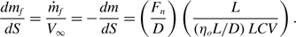 \begin{align}\frac{{d{m_f}}}{{dS}} = \frac{{{{\dot m}_f}}}{{{V_\infty }}} = - \frac{{dm}}{{dS}} = \left( {\frac{{{F_n}}}{D}} \right)\left( {\frac{L}{{\left( {{\eta _o}L/D} \right)LCV}}} \right).\end{align}
Here m is the instantaneous total mass of the aircraft, S is the distance travelled through the air, L is the lift and D is the drag.
In the steady state cruise, lift is equal to weight and thrust is equal to dragFootnote 2 . Hence,
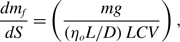 \begin{align}\frac{{d{m_f}}}{{dS}} = \left( {\frac{{mg}}{{\left( {{\eta _o}L/D} \right)LCV}}} \right),\end{align}
where g is the acceleration due to gravity. Therefore, the rate at which fuel is consumed in cruise is governed by the single aero-thermodynamic parameter $(\eta_{o}L/D)$
. Dimensional analysis reveals that, in general, this quantity is a function of the flight Mach number,
$(\eta_{o}L/D)$
. Dimensional analysis reveals that, in general, this quantity is a function of the flight Mach number, $M^{\infty}$
, and the flight Reynolds number,
$M^{\infty}$
, and the flight Reynolds number, $R^{ac}$
. Following Poll and Schumann [2], Reynolds number is defined as
$R^{ac}$
. Following Poll and Schumann [2], Reynolds number is defined as
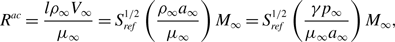 \begin{align}{R^{ac}} = \frac{{l{\rho _\infty }{V_\infty }}}{{{\mu _\infty }}} = S_{ref}^{1/2}\left( {\frac{{{\rho _\infty }{a_\infty }}}{{{\mu _\infty }}}} \right){M_\infty } = S_{ref}^{1/2}\left( {\frac{{\gamma {p_\infty }}}{{{\mu _\infty }{a_\infty }}}} \right){M_\infty },\end{align}
whilst the aircraft lift, drag and thrust coefficients have their usual definitions, i.e.
 \begin{align}{C_L} = \frac{L}{{{q_\infty }{S_{ref}}}}\;,\;{C_D} = \frac{D}{{{q_\infty }{S_{ref}}}}{\rm{\;and\;}}{C_T} = \frac{{{F_n}}}{{{q_\infty }{S_{ref}}}}\;\;{\rm{where}}\;{q_\infty } = \frac{\gamma }{2}\;{p_\infty }M_\infty ^2.\end{align}
Here, air is taken to be an ideal gas, l is a “typical” aircraft reference length, taken to be the square root of the reference wing area, S
ref
, p
∞
is the atmospheric static pressure, $\rho$
∞
the density, a
∞
the local speed of sound, μ
∞
the dynamic viscosity and γ is the ratio of specific heats.
$\rho$
∞
the density, a
∞
the local speed of sound, μ
∞
the dynamic viscosity and γ is the ratio of specific heats.
In practise, aircraft do not cruise at a fixed altitude. Rather, to maintain safe separation in the vertical direction, they follow isobars, i.e. they fly in such a way that the local static pressure, p ∞ , is held constant. By international agreement, values of static pressure are converted into “flight levels”, which are the altitudes, measured in feet, that the aircraft would have if it was operating in the International Standard Atmosphere (ISA) [6] divided by 100 feet.
3.0 Conditions for optimum (
$\eta$
o
L/D) and the design optimum

In Poll [1] it was shown that, for an aircraft with a specified mass and Mach number in steady, straight and level flight, there is a lift coefficient, (C
L
)
B
, at which ( $\eta$
o
L/D) has a local maximum, or best, value. Furthermore, there is a particular combination of Mach number, M
o
, and lift coefficient, (C
L
)
o
, at which (
$\eta$
o
L/D) has a local maximum, or best, value. Furthermore, there is a particular combination of Mach number, M
o
, and lift coefficient, (C
L
)
o
, at which ( $\eta$
o
L/D) has an absolute maximum, or optimum, value, i.e. the fuel burn per unit distance travelled through the air has an absolute minimum.
$\eta$
o
L/D) has an absolute maximum, or optimum, value, i.e. the fuel burn per unit distance travelled through the air has an absolute minimum.
The conditions for optimum ( $\eta$
o
L/D) are determined by a balance between the gradients of
$\eta$
o
L/D) are determined by a balance between the gradients of $\eta$
o
and L/D with respect to both Mach number, M
∞
, and either flight level, or p
∞
, i.e. when
$\eta$
o
and L/D with respect to both Mach number, M
∞
, and either flight level, or p
∞
, i.e. when
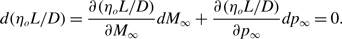 \begin{align}d\!\left( {{\eta _o}L/D} \right) = \frac{{\partial \!\left( {{\eta _o}L/D} \right)}}{{\partial {M_\infty }}}d{M_\infty } + \frac{{\partial \!\left( {{\eta _o}L/D} \right)}}{{\partial {p_\infty }}}d{p_\infty } = 0.\end{align}
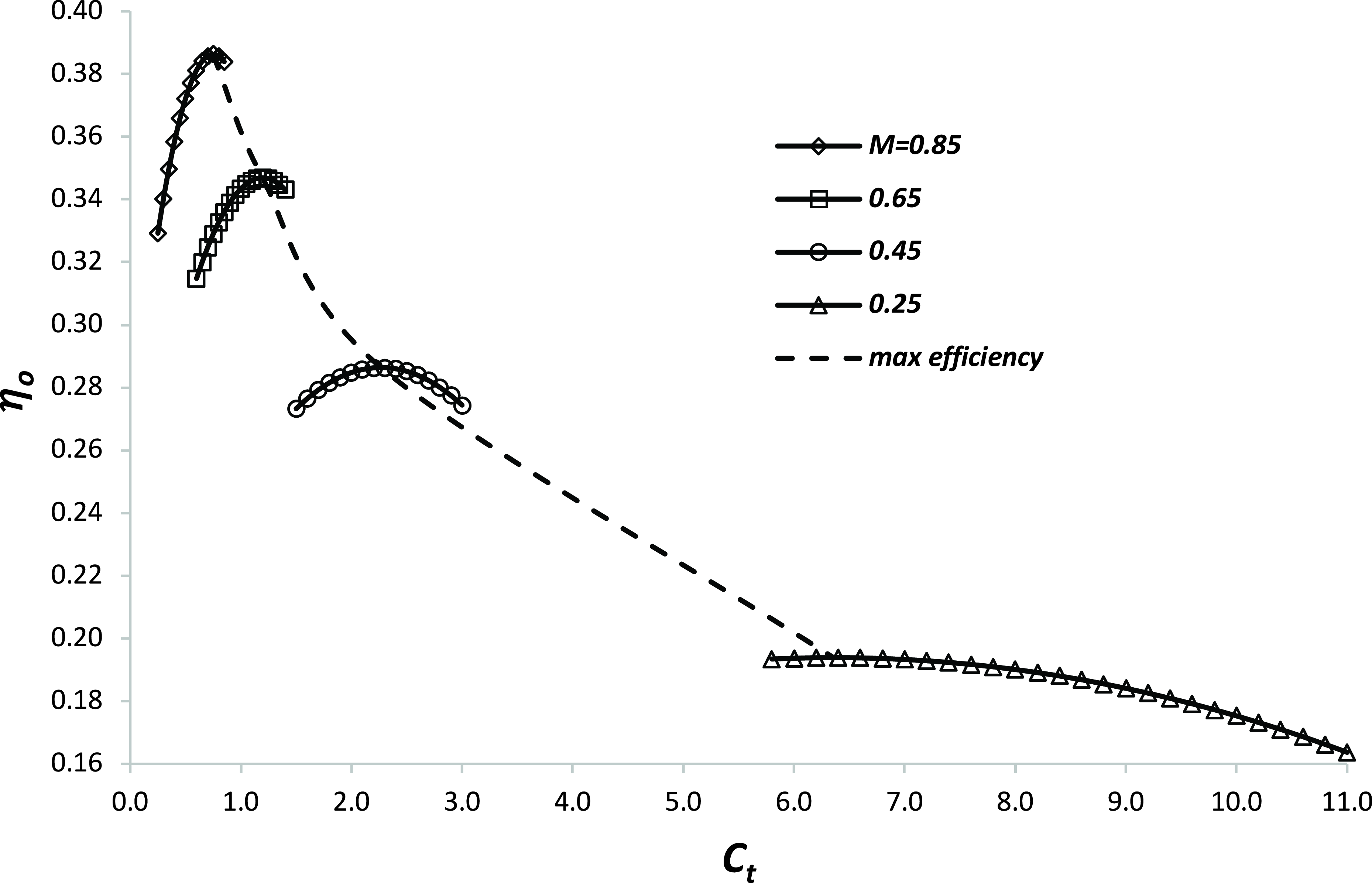
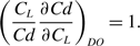
The variation of overall efficiency with thrust coefficient and Mach number for a civil aircraft turbofan engine with a nominal bypass ratio of 8. Data taken from Jenkinson et al [Reference Jenkinson, Simpkin and Rhodes7].
In straight and level flight, thrust is equal to drag and, from the definition of lift coefficient,
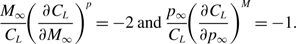 \begin{align}\;\frac{{{M_\infty }}}{{{C_L}}}{\!\left( {\frac{{\partial {C_L}}}{{\partial {M_\infty }}}} \right)^p} = - 2\;{\rm{and\;}}\frac{{{p_\infty }}}{{{C_L}}}{\!\left( {\frac{{\partial {C_L}}}{{\partial {p_\infty }}}} \right)^M} = - 1.\;\end{align}
Therefore, Equation (6) is satisfied when
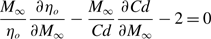 \begin{align}\frac{{{M_\infty }}}{{{\eta _o}}}\frac{{\partial {\eta _o}}}{{\partial {M_\infty }}} - \frac{{{M_\infty }}}{{Cd}}\frac{{\partial Cd}}{{\partial {M_\infty }}} - 2 = 0\end{align}
and
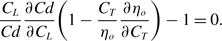 \begin{align}\frac{{{C_L}}}{{Cd}}\frac{{\partial Cd}}{{\partial {C_L}}}\!\left( {1 - \frac{{{C_T}}}{{{\eta _o}}}\frac{{\partial {\eta _o}}}{{\partial {C_T}}}} \right) - 1 = 0.\end{align}
As discussed in Poll and Schumann [Reference Poll3] and as shown in Fig. 1, at fixed M
∞
, engine overall efficiency, $\eta$
o
, has a local maximum value at a particular value of the thrust coefficient, C
T
. This maximum is strongly dependent upon the Mach number and, provided that M
∞
is greater than 0.2Footnote
3
may be represented by a power law, i.e. when
$\eta$
o
, has a local maximum value at a particular value of the thrust coefficient, C
T
. This maximum is strongly dependent upon the Mach number and, provided that M
∞
is greater than 0.2Footnote
3
may be represented by a power law, i.e. when
 \begin{align}\frac{{{C_T}}}{{{\eta _o}}}\frac{{\partial {\eta _o}}}{{\partial {C_T}}} = 0,\end{align}
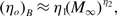 \begin{align}{\left( {{\eta _o}} \right)_B} \approx {\eta _1}{\!\left( {{M_\infty }} \right)^{{\eta _2}}},\end{align}
where the coefficients $\eta_{1}$
and
$\eta_{1}$
and $\eta_{2}$
are constant and depend upon the engine type. It follows that
$\eta_{2}$
are constant and depend upon the engine type. It follows that
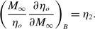 \begin{align}{\left( {\frac{{{M_\infty }}}{{{\eta _o}}}\frac{{\partial {\eta _o}}}{{\partial {M_\infty }}}} \right)_B} = {\eta _2}.\end{align}
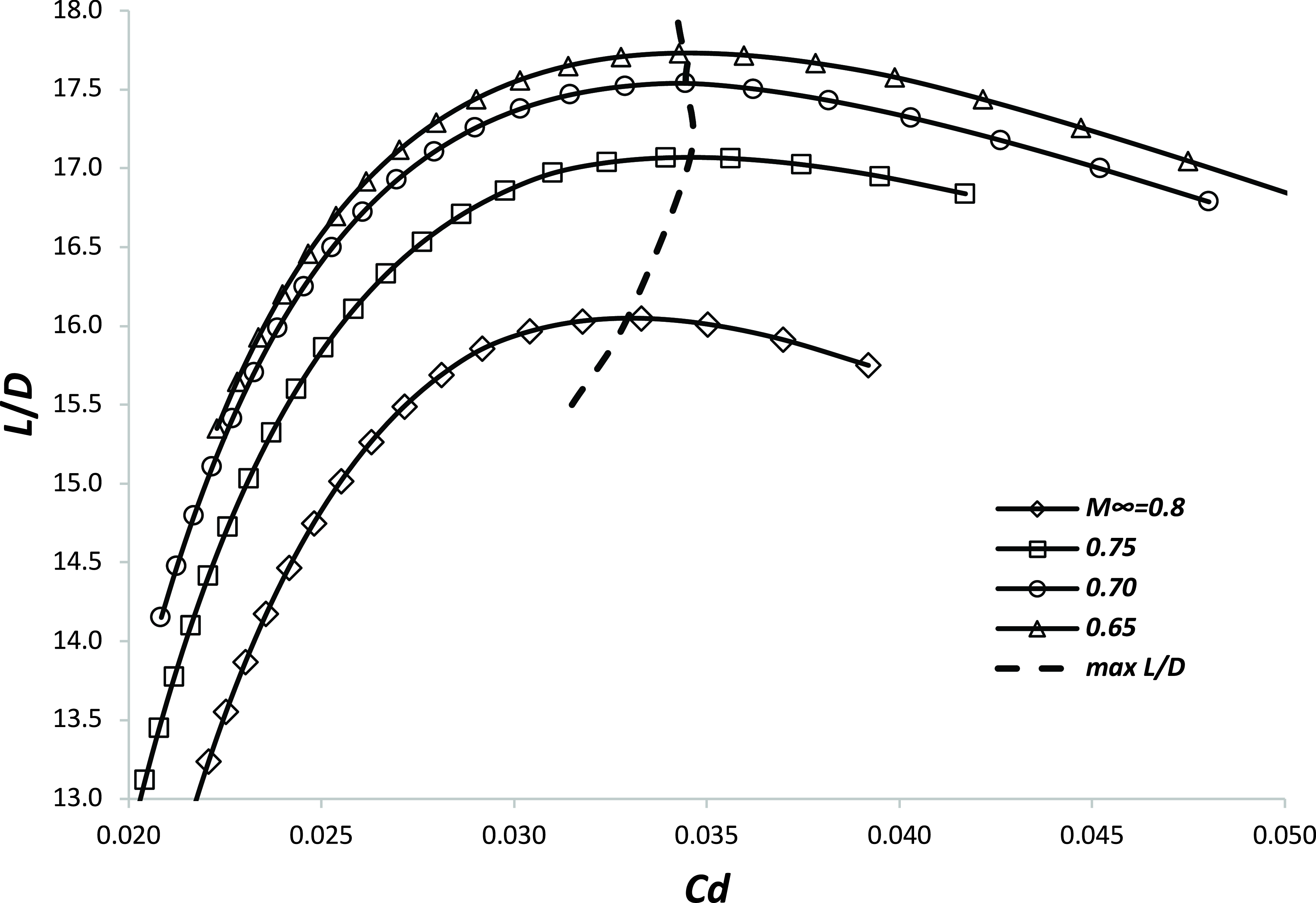
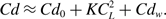
Similarly, as shown in Fig. 2, when the mass and Mach number are fixed, the aircraft lift-to-drag ratio has a local maximum at a particular value of the drag coefficient. However, in this case, the maximum L/D reduces as Mach number increases.
An example of the variation of aircraft lift-to-drag ratio with drag coefficient and Mach number when the mass is fixed.
In order to have the absolute maximum value of ( $\eta$
o
L/D) the airframe and engine must be “perfectly” matched, i.e. both
$\eta$
o
L/D) the airframe and engine must be “perfectly” matched, i.e. both $\eta$
o
and L/D must have local maxima at the same values of Mach number and drag (= thrust) coefficient. However, this can only be achieved at a single condition. Hence, for specified mass and a specified atmosphere, there is only one possible combination of Mach number and Reynolds number. Since this condition is fixed in the design process, it is appropriate to call it the “design optimum” condition, and the corresponding flight condition is a characteristic of the airframe-engine combination. Hence, at the design optimum, Equations (8) and (9) become
$\eta$
o
and L/D must have local maxima at the same values of Mach number and drag (= thrust) coefficient. However, this can only be achieved at a single condition. Hence, for specified mass and a specified atmosphere, there is only one possible combination of Mach number and Reynolds number. Since this condition is fixed in the design process, it is appropriate to call it the “design optimum” condition, and the corresponding flight condition is a characteristic of the airframe-engine combination. Hence, at the design optimum, Equations (8) and (9) become
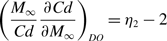 \begin{align}{\left( {\frac{{{M_\infty }}}{{Cd}}\frac{{\partial Cd}}{{\partial {M_\infty }}}} \right)_{DO}} = {\eta _2} - 2\end{align}
and
 \begin{align}{\left( {\frac{{{C_L}}}{{Cd}}\frac{{\partial Cd}}{{\partial {C_L}}}} \right)_{DO}} = 1.\end{align}
These are completely general relations that define the design optimum value of ( $\eta$
o
L/D) in any specified design atmosphere and the conditions at which it occurs.
$\eta$
o
L/D) in any specified design atmosphere and the conditions at which it occurs.
4.0 Estimation of the drag
If Equations (13) and (14) are to be solved, it is necessary to know the relation linking the drag coefficient to the lift coefficient and Mach number, otherwise known as the aircraft’s “drag polar”. For Mach numbers greater than 0.5, the cruise drag coefficient may be expressed in the form proposed by Shevell [Reference Shevell8], i.e.
 \begin{align}Cd \approx C{d_0} + KC_L^2 + C{d_w}.\end{align}
The first term, Cd
0
, is the zero-lift drag coefficient and the standard approximation is that this is directly proportional to the aircraft’s mean skin-friction coefficient, $C_F^{ac}$
. Hence,
$C_F^{ac}$
. Hence,
 \begin{align}C{d_0} = {\psi _0}C_F^{ac},\end{align}
where $\psi_{0}$
depends upon the aircraft geometry. In general,
$\psi_{0}$
depends upon the aircraft geometry. In general, $Cd_{0}$
also depends upon
$Cd_{0}$
also depends upon $M_{\infty}$
. This is because increasing the Mach number increases surface temperatureFootnote
4
and modifies the surface pressure distribution. The result is that skin friction reduces and the pressure, or ‘form’, drag increases, i.e. the constant of proportionality linking
$M_{\infty}$
. This is because increasing the Mach number increases surface temperatureFootnote
4
and modifies the surface pressure distribution. The result is that skin friction reduces and the pressure, or ‘form’, drag increases, i.e. the constant of proportionality linking $Cd_{0}$
and
$Cd_{0}$
and $(C_{F}^{ac})$
increases. However, for Mach numbers above 0.5, the net effect is a cancellation making
$(C_{F}^{ac})$
increases. However, for Mach numbers above 0.5, the net effect is a cancellation making $Cd_{0}$
approximately independent of Mach number, see Shevell [Reference Shevell8] (Chapter 12). Poll and Schumann [2] have shown that the relationship between skin friction and Reynolds number, at a Mach number of 0.5, can be approximated by the power law
$Cd_{0}$
approximately independent of Mach number, see Shevell [Reference Shevell8] (Chapter 12). Poll and Schumann [2] have shown that the relationship between skin friction and Reynolds number, at a Mach number of 0.5, can be approximated by the power law
 \begin{align}C_F^{ac} \approx \frac{a}{{{{\left( {{R^{ac}}} \right)}^b}}},\end{align}
where a and b are constants having values of 0.0269 and 0.14, respectively.
The second term, K, is known as the low-speed, lift-dependent drag factor, and is given by
 \begin{align}K = \frac{1}{{\pi .AR.{e_{LS}}}}.\end{align}
Here, AR is the wing aspect ratio, defined as
 \begin{align}AR = \frac{{{s^2}}}{{{S_{ref}}}},\end{align}
where s is the wingspan and $e_{LS}$
is the low-speed Oswald efficiency factor.
$e_{LS}$
is the low-speed Oswald efficiency factor.
The Oswald factor captures all the lift-dependent drag effects of which vortex drag on the wings is the primary source. However, the tailplane and the fuselage also generate vortex drag. In addition, there are non-vortex, lift-dependent drag contributions arising because a change in lift alters the pressure distribution over the various components, which, in turn, alters their profile drag. Therefore, the Oswald factor is complex and, as explained by Shevell [6], it is primarily a function of aircraft geometry and Cd 0 and is given, approximately, by
 \begin{align}\;{e_{LS}} \approx \frac{1}{{{\delta _1} + {\delta _2} + \pi .AR.{k_1}}}.\end{align}
Again following Shevell, $\delta$
1 is a constant representing the wing vortex drag and is typically about 1.03, whilst
$\delta$
1 is a constant representing the wing vortex drag and is typically about 1.03, whilst $\delta$
2 represents the interference effect between the wing and the fuselage, which may be approximated by
$\delta$
2 represents the interference effect between the wing and the fuselage, which may be approximated by
 \begin{align}{\delta _2} \approx 2{\!\left( {\frac{{{b_f}}}{s}} \right)^2},\end{align}
with b f being the fuselage maximum width and k 1 is the non-vortex, lift dependent drag factor, where, as discussed in Poll and Schumann [Reference Poll3]
 \begin{align}\;{k_1} \approx 0.80\!\left( {1 - 0.53\;cos\!\left( {{\Lambda _w}} \right)} \right)\!C{d_0},\end{align}
and $\Lambda_{w}$
the wing quarter-chord sweep angle. Hence,
$\Lambda_{w}$
the wing quarter-chord sweep angle. Hence,
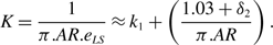 \begin{align}\;K = \frac{1}{{\pi .AR.{e_{LS}}}} \approx {k_1} + \left( {\frac{{1.03 + {\delta _2}}}{{\pi .AR}}} \right).\end{align}
Finally, the third term, Cd w , is the “wave drag” coefficient. For an aerofoil at a given angle-of-attack, as the flight speed increases from a low starting value, sonic conditions will eventually be reached at the point on the surface where the local static pressure is lowest. Usually, this point is close to the leading edge on the wing’s upper surface and the corresponding flight Mach number is called the “critical” value, M crit . Further increases in speed result in the formation of a region of supersonic flow that is bounded by the wing surface, a “sonic interface”Footnote 5 and, if the Mach number is sufficiently high, a terminating shockwave. Once a “supersonic zone” is established, increases in either M ∞ , or C L, produce an increase in drag and the terminating shockwave moves rearwards. When this zone is confined to the front portion of the wing, the drag increases are modest, being typically less than 10 drag countsFootnote 6 – see, for example, Torenbeek [Reference Torenbeek9] (Section 4.6). Consequently, the variation is known as “drag creep”. However, when the terminating shockwave moves onto the rear part of the wing, the rate of drag rise with increasing Mach number, or increasing C L , becomes large and this is usually referred to as “drag rise”. Since both the creep and rise regimes are linked to the formation and subsequent development of shockwaves, the resulting drag increments are collectively referred to as “wave” drag.
In the current approach, since, by definition, both Cd 0 and K are independent of Mach number, Cd w captures all the additional effects due to compressibility and, once this is specified as a function of Mach number and lift coefficient, the drag polar is complete.
As shown in detail in Appendix A, the conditions at the design optimum condition are obtained by differentiating the drag polar and, after some manipulation, it is found that, to a very good approximation, in a completely general atmosphere, the design optimum values for C L , Cd and L/D are given by
 \begin{align}{\left( {{C_L}} \right)_{DO}} \approx \!\left( {1 - {1 \over 2}\!\left( {b\!\left( {1 + \left( {{{{k_1}} \over K}} \right)} \right)\left( {1 + {{\rm{\Gamma }}_{DO}}} \right) + {{\left( {{{C{d_w}} \over {C{d_0}}}} \right)}_{DO}}\!\left( {{{\left( {{{{C_L}} \over {C{d_{}}}}{{\partial C{d_w}} \over {\partial {C_L}}}} \right)}_{DO}} - 1} \right)} \right)} \right)\left( {{{C{d_0}} \over K}} \right)_{DO}^{1/2}\end{align}
and, using equation (15),
 \begin{align}{\left( {Cd} \right)_{DO}} \approx 2\!\left( {1 - \frac{1}{2}\!\left( {b\!\left( {1 + \left( {\frac{{{k_1}}}{K}} \right)} \right)\left( {1 + {{\rm{\Gamma }}_{DO}}} \right) + {{\left( {\frac{{C{d_w}}}{{C{d_0}}}} \right)}_{DO}}\!\left( {{{\left( {\frac{{{C_L}}}{{C{d_w}}}\frac{{\partial C{d_w}}}{{\partial {C_L}}}} \right)}_{DO}} - 2} \right)} \right)} \right){\left( {C{d_0}} \right)_{DO}}.\;\end{align}
Hence,
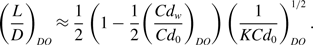 \begin{align}{\left( {{L \over D}} \right)_{DO}} \approx {1 \over 2}\left( {1 - {1 \over 2}{{\left( {{{C{d_w}} \over {C{d_0}}}} \right)}_{DO}}} \right)\left( {{1 \over {KC{d_0}}}} \right)_{DO}^{1/2}.\end{align}
Provided that Equation (15) is used as the definition for Cd
w
, these relations show how the wave drag, the Reynolds number and the atmospheric parameters affect the values of C
L
, Cd and L/D when ( $\eta$
o
L/D) is at its design optimum value.
$\eta$
o
L/D) is at its design optimum value.
5.0 Representation of the wave drag
Wave drag is a very complex phenomenon, but, under normal cruising conditions, it accounts for only about 3% of the total, see Torenbeek [Reference Torenbeek9] (Fig. 14.6). Nevertheless, its strong dependence upon Mach number and lift coefficient means that it has an influence on the aircraft’s maximum lift-to-drag ratio and the flight conditions at which this occurs. Accurate, simple models of wave drag are rare. However, there is one method that captures enough of the underlying physics to provide a reasonably accurate, qualitative and quantitative description of the process.
Based on the experimentally determined drag characteristics of early, two-dimensional, transonic aerofoil sections, Shevell, [Reference Shevell8] but see also Shevell and Bayan [Reference Shevell and Bayan10] and Shevell, [Reference Shevell11] suggested that, whilst “drag creep” develops when M ∞ exceeds M crit , the onset of “drag rise” is linked to the establishment of sonic conditions at the aerofoil “crest”. This is the point on the aerofoil’s upper surface that is parallel to the free-stream direction and locally sonic conditions are established there when M ∞ reaches the “crest critical” Mach number, M cc . Shevell observed that M cc depends, primarily, upon wing geometry and the lift coefficient, whilst the wave drag coefficient itself is governed by the ratio of M ∞ to M cc .
Shevell proposed a method for estimating M cc from a knowledge of the mean thickness-to-chord ratio and C L. Unfortunately, it is both complex and implicit. However, as can be seen in Ref. [Reference Poll and Schumann5] (Fig. 12.7), for the ranges of thickness-to-chord ratio, t/c, and lift coefficient of practical interest, M cc may be adequately represented by the relation
 \begin{align}{\left( {{M_{CC}}} \right)_{2 - D}} \approx 0.88 - 0.18{\left( {{C_L}} \right)_{2 - D}} - 0.92\left( {t/c} \right).\end{align}
This result applies to aerofoils with “peaky” pressure distributions, i.e. those having a very low pressure in a narrow region on the upper surface very close to the leading edge, that were typical of the high-speed aerofoil designs developed in the 1960s and 1970s.
An important application of Shevell’s method is the determination of the aerofoil’s drag “divergence” Mach number, M
DD
. This is the value above which the drag is deemed, somewhat arbitrarily, to increase very rapidly with increasing flight Mach number. For historical reasons, there are two definitions for M
DD
in general use. The first, introduced by the Douglas Aircraft Company, is the Mach number at which, for a fixed lift coefficient, the gradient $\partial$
Cd/
$\partial$
Cd/ $\partial$
M
∞
reaches a specified value. Depending on the aerofoil, this may be either 0.05 or 0.1. The second is the Mach number that gives a fixed drag increase relative to the incompressible value for the same lift coefficient, i.e. a specific increment in Cd
w
. According to Raymer, [Reference Raymer12] the Boeing Company has used this definition, with the drag increment taken to be 20 counts. Clearly, when the Mach number is close to M
DD
, the drag coefficient will be rising rapidly and these three criteria will yield similar results, with Shevell’s relations suggesting that
$\partial$
M
∞
reaches a specified value. Depending on the aerofoil, this may be either 0.05 or 0.1. The second is the Mach number that gives a fixed drag increase relative to the incompressible value for the same lift coefficient, i.e. a specific increment in Cd
w
. According to Raymer, [Reference Raymer12] the Boeing Company has used this definition, with the drag increment taken to be 20 counts. Clearly, when the Mach number is close to M
DD
, the drag coefficient will be rising rapidly and these three criteria will yield similar results, with Shevell’s relations suggesting that
 \begin{align}{\left( {\frac{{{{\left( {{M_{DD}}} \right)}_{20}}}}{{{M_{CC}}}}} \right)_{2 - D}} \approx 1.03,\;{\left( {\frac{{{{\left( {{M_{DD}}} \right)}_{0.05}}}}{{{M_{CC}}}}} \right)_{2 - D}} \approx 1.02\;{\rm{and}}\;{\left( {\frac{{{{\left( {{M_{DD}}} \right)}_{0.1}}}}{{{M_{CC}}}}} \right)_{2 - D}} \approx 1.045.\end{align}
The significant point of note is that M DD and M cc are related by a simple factor that is close to unity. This implies that the qualitative physical argument for M cc and Shevell’s complex, first principles, estimation method is neither necessary, nor does it even need to be valid, since M cc can just be viewed as a simple reference Mach number for the onset of drag rise. Hence, if the divergence Mach number is known for a given aerofoil section, it can be used to estimate the corresponding value of M cc . This is fortuitous, since M DD has received more attention in the open literature than M cc . Consequently, the modified “Shevell method” may be applied to any aerofoil whose divergence Mach number is known.
The “peaky” aerofoil sections used in the original analysis were superseded by the much improved “supercritical” designs with higher intrinsic values of M DD and reduced sensitivity to changes in C L . The general behaviour of more modern aerofoils is given by the well-known “Korn” equation, which appears in many references, e.g. Torenbeek [Reference Torenbeek9], Mason [Reference Mason13] and Boppe [Reference Boppe14] and is
 \begin{align}{\left( {{{\left( {{M_{DD}}} \right)}_{0.1}}} \right)_{2 - D}} \approx {M_{TF}} - 0.10{\left( {{C_L}} \right)_{2 - D}} - 1.00\left( {t/c} \right),\end{align}
where $M_{TF}$
is a constant “aerofoil technology” factor. Shevell [Reference Shevell8] suggests that, for supercritical aerofoils,
$M_{TF}$
is a constant “aerofoil technology” factor. Shevell [Reference Shevell8] suggests that, for supercritical aerofoils, $M_{TF}$
falls in the range of 0.93 to 0.97, which is consistent with the average value of 0.95 quoted by Mason[Reference Shevell11].
$M_{TF}$
falls in the range of 0.93 to 0.97, which is consistent with the average value of 0.95 quoted by Mason[Reference Shevell11].
Whilst the arguments behind the method are based upon 2-D aerofoil characteristics, the governing relations may be extended to cover swept wings of infinite span by applying the standard “infinite sheared wing” transformation. This means that streamwise aerofoil section geometry is held constant as the sweep angle, $\Lambda$
w
, is increased, whilst allowing no variation of any geometric characteristic, or flow property, in the direction parallel to the leading edge. Using the results from Equations (28) and (29), the extended model becomes
$\Lambda$
w
, is increased, whilst allowing no variation of any geometric characteristic, or flow property, in the direction parallel to the leading edge. Using the results from Equations (28) and (29), the extended model becomes
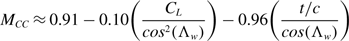 \begin{align}{M_{CC}} \approx 0.91 - 0.10\!\left( {\frac{{{C_L}}}{{co{s^2}\!\left( {{\Lambda _w}} \right)}}} \right) - 0.96\!\left( {\frac{{t/c}}{{cos\!\left( {{\Lambda _w}} \right)}}} \right)\end{align}
and
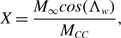 \begin{align}X = \frac{{{M_\infty }cos\!\left( {{\Lambda _w}} \right)}}{{{M_{CC}}}},\end{align}
where
 \begin{align}C{d_w} \approx co{s^3}\!\left( {{\Lambda _w}} \right)function\!\left( X \right).\end{align}
These expressions are exact for an isolated, infinite-swept wing, but, on a full aircraft configuration, wave drag could also develop on the fuselage and other surfaces. However, as noted by Shevell [Reference Shevell8] on a “well-designed” aircraft, the wave drag will always be dominated by the contribution from the wing and it will be assumed that all the aircraft to be considered in this study are “well designed”.
On an aircraft wing, the span is finite and, in general, the local lift, streamwise chord, aerofoil section and twist will all vary in the spanwise direction. In addition, the fuselage influences the wing flow by modifying both the spanwise lift distribution and the local freestream velocity. All these effects influence wave drag development. Nevertheless, since most of the wave drag will be generated by the wing, by using the aircraft’s total lift coefficient, an “average” value for t/c and taking $\Lambda$
w
to be measured at the mean ¼ chord line, Equations (30), (31) and (32) can still provide the basis for a reasonable approximation of the wave drag for a complete aircraft configuration.
$\Lambda$
w
to be measured at the mean ¼ chord line, Equations (30), (31) and (32) can still provide the basis for a reasonable approximation of the wave drag for a complete aircraft configuration.
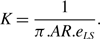
High Mach number drag data for total aircraft configurations rarely appear in the open literature. However, Obert [Reference Obert15] (Chapter 24) gives some useable information on the variation of drag coefficient with Mach number at various, fixed values of lift coefficient for thirteen civil transport aircraft. It is not always clear where these data have come from, or how accurate they are, and all are presented in very small figures. Nevertheless, divergence Mach number data for the aircraft’s “average” aerofoil section have been extracted by assuming that pressure related drag acts in the direction normal to the ¼ chord line and applying the “20 additional drag counts” definition in that plane. The results are given in Fig. 3.
The approximate variation of mean aerofoil, drag divergence Mach number with aircraft total lift coefficient for a range of aircraft types. Data are taken from Obert [Reference Obert15]. The solid line is Equation (33), the heavy dashed lines indicate ± 7% deviation and the light dashed lines show the trend for each individual aircraft.
In every case, M DD decreases as the total aircraft C L increases and, using a straight line fit, slope and intercept values were obtained for each case. Averaging these gives
 \begin{align}{M_{DD}} \approx 0.76 - 0.11\!\left( {\frac{{{C_L}}}{{co{s^2}\!\left( {{\Lambda _w}} \right)}}} \right)\end{align}
and, using equation (28), it follows that, for the full aircraft configuration,
 \begin{align}{\left( {{M_{cc}}} \right)^{ac}} = {\left( {{M_{TF}}} \right)^{ac}} - 0.10\!\left( {\frac{{{C_L}}}{{co{s^2}\!\left( {{\Lambda _w}} \right)}}} \right) \approx 0.74 - 0.10\!\left( {\frac{{{C_L}}}{{co{s^2}\!\left( {{\Lambda _w}} \right)}}} \right).\end{align}
where $(M_{TF})^{ac}$
is a constant that captures the aerofoil technology factor plus the effect of the wing thickness-to-chord ratio and, consequently, is a characteristic of the aircraft. As indicated in Fig. 3, the average factor of 0.74 is subject to an uncertainty of at least
$(M_{TF})^{ac}$
is a constant that captures the aerofoil technology factor plus the effect of the wing thickness-to-chord ratio and, consequently, is a characteristic of the aircraft. As indicated in Fig. 3, the average factor of 0.74 is subject to an uncertainty of at least $\pm$
7%. However, most importantly, the data suggest that the gradient
$\pm$
7%. However, most importantly, the data suggest that the gradient $dM_{CC}/dC_{L}$
for the full aircraft configuration is close to that for the wing in isolation.
$dM_{CC}/dC_{L}$
for the full aircraft configuration is close to that for the wing in isolation.
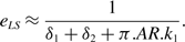
Finally, Shevell [Reference Shevell8] (Fig. 12.13) gives a single, empirical curve for the approximate variation of total aircraft Cd w with the parameter X and this is given in Fig. 4.
The variation of wave drag coefficient with the characteristic parameter X - solid line is the original Shevell [Reference Shevell8] curve, dotted line is Equation (36) and the dashed line is Equation (38) with j 1 and j 2 being set to 0.080 and 0.875, respectively.
For the analysis carried out in Poll and Schumann [Reference Poll3], Shevell’s curve was represented by the relation
 \begin{align}{\left( {C{d_w}} \right)_{creep}} \approx co{s^3}\!\left( {{{\rm{\Lambda }}_w}} \right)\left( {0.016{{\left( {X - 0.75} \right)}^2}} \right),\end{align}
for X less than 0.92 and for larger values
 \begin{align}{\left( {C{d_w}} \right)_{rise}} \approx co{s^3}\!\left( {{{\rm{\Lambda }}_w}} \right)\left( {0.016{{\left( {X - 0.75} \right)}^2} + 6.5{{\left( {X - 0.92} \right)}^4}} \right).\end{align}
The form of the additional term in the drag “rise” variation was chosen to reflect the “ideal” drag rise due solely to the presence of a normal shock wave in the flow as derived by Lock [Reference Lock16], i.e.
 \begin{align}{\left( {C{d_w}} \right)_{shock}} \propto co{s^3}\!\left( {{{\rm{\Lambda }}_w}} \right){\left( {{M_\infty }\cos \!\left( {{{\rm{\Lambda }}_w}} \right) - constant} \right)^4}.\end{align}
Equation (36) is included in Fig. 4 and it is a reasonable approximation to the Shevell curve for values of X up to 1.05.
6.0 Estimation of the characteristics at the design optimum condition
Clearly, if an aircraft flies at a Mach number greater than the drag divergence Mach number of the wing’s aerofoil sections, there will be a significant fuel penalty. Hence, in practice and mainly for reasons of economy, the largest operational value is usually the long-range cruise Mach number, M LRC . Furthermore, Poll [1] (Equation (24)) has estimated that the Mach number for absolute minimum fuel burn, M o , is about 3.5% lower than M LRC and that the corresponding wave drag coefficient is less than 10 drag counts. This suggests that the optimum condition is likely to occur at the top end of the drag creep region, i.e. at a value of X that is close to unity. In this region, Equation (36) is both complex and not a particularly good match to the gradients of Shevell’s original curve. Therefore, to simplify the analysis and improve the accuracy, the wave drag coefficient in the region of the optimum is given by the local approximation,
 \begin{align}\frac{{C{d_w}}}{{co{s^3}\!\left( {{{\rm{\Lambda }}_w}} \right)}} \approx {j_1}{\!\left( {X - {j_2}} \right)^2},\end{align}
where $j_{1}$
and
$j_{1}$
and $j_{2}$
are constants. By matching the value and gradient of the Shevell curve when X is unity,
$j_{2}$
are constants. By matching the value and gradient of the Shevell curve when X is unity, $j_{1}$
and
$j_{1}$
and $j_{2}$
are found to be 0.080 and 0.875 respectively. This curve is also shown in Fig. 4 and the agreement is very good for X in the range 0.97 to 1.02.
$j_{2}$
are found to be 0.080 and 0.875 respectively. This curve is also shown in Fig. 4 and the agreement is very good for X in the range 0.97 to 1.02.
Hence, using Equations (24) and (38), at the design condition,
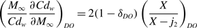 \begin{align}{\!\left( {\frac{{{M_\infty }}}{{C{d_w}}}\frac{{\partial C{d_w}}}{{\partial {M_\infty }}}} \right)_{DO}} = 2\!\left( {1 - {\delta _{DO}}} \right){\left( {\frac{X}{{X - {j_2}}}} \right)_{DO}}\end{align}
and
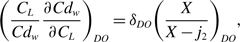 \begin{align}{\left( {\frac{{{C_L}}}{{C{d_w}}}\frac{{\partial C{d_w}}}{{\partial {C_L}}}} \right)_{DO}} = {\delta _{DO}}{\left( {\frac{X}{{X - {j_2}}}} \right)_{DO}},\end{align}
where
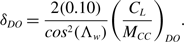 \begin{align}{\delta _{DO}} = \frac{{2\!\left( {0.10} \right)}}{{co{s^2}\!\left( {{{\rm{\Lambda }}_w}} \right)}}{\left( {\frac{{{C_L}}}{{{M_{CC}}}}} \right)_{DO}}.\end{align}
Using Equations (A-15) and (A-16) from Appendix A, it can be shown that the optimum values of the lift coefficient and the wave drag coefficient are related directly, i.e.
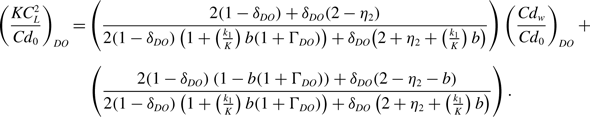 \begin{align}\left( \frac{KC_{L}^{2}}{{Cd}_{0}} \right)_{DO} &= \left( \frac{2\!\left( 1 - \delta_{DO} \right) + \delta_{DO}\!\left( 2 - \eta_{2} \right)}{2\!\left( 1 - \delta_{DO} \right)\left( 1 + \left( \frac{k_{1}}{K} \right)b\!\left( 1 + \Gamma_{DO} \right) \right) + \delta_{DO}\!\left( 2 + \eta_{2} + \left( \frac{k_{1}}{K} \right)b \right)} \right)\left( \frac{{Cd}_{w}}{{Cd}_{0}} \right)_{DO} +\nonumber \\[5pt]&\quad \left( {\frac{{2\!\left( {1 - {\delta _{DO}}} \right)\left( {1 - b\!\left( {1 + {{\rm{\Gamma }}_{DO}}} \right)} \right) + {\delta _{DO}}\!\left( {2 - {\eta _2} - b} \right)}}{{2\!\left( {1 - {\delta _{DO}}} \right)\left( {1 + \left( {\frac{{{k_1}}}{K}} \right)b\!\left( {1 + {{\rm{\Gamma }}_{DO}}} \right)} \right) + {\delta _{DO}}\left( {2 + {\eta _2} + \left( {\frac{{{k_1}}}{K}} \right)b} \right)}}} \right).\end{align}
Since $\delta$
DO
depends upon (C
L
)
DO
, this is an implicit expression for (C
L
)
DO
that can only be solved by iteration. Consequently, approximate solutions will be developed.
$\delta$
DO
depends upon (C
L
)
DO
, this is an implicit expression for (C
L
)
DO
that can only be solved by iteration. Consequently, approximate solutions will be developed.
As shown in Appendix B, over the parameter ranges of practical interest, after some manipulation, further approximation and curve fitting, it is found that the wave drag coefficient is well represented by
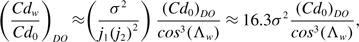 \begin{align}{\left( {\frac{{C{d_w}}}{{C{d_0}}}} \right)_{DO}} \approx \!\left( {\frac{{{\sigma ^2}}}{{{j_1}{{\left( {{j_2}} \right)}^2}}}} \right)\frac{{{{\left( {C{d_0}} \right)}_{DO}}}}{{co{s^3}\!\left( {{{\rm{\Lambda }}_w}} \right)}} \approx 16.3{\sigma ^2}\frac{{{{\left( {C{d_0}} \right)}_{DO}}}}{{co{s^3}\!\left( {{{\rm{\Lambda }}_w}} \right)}},\end{align}
where $j_{1}$
and
$j_{1}$
and $j_{2}$
have been taken to be 0.080 and 0.875, respectively, and
$j_{2}$
have been taken to be 0.080 and 0.875, respectively, and
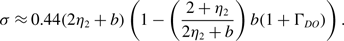 \begin{align}\sigma \approx 0.44\!\left( {2{\eta _2} + b} \right)\left( {1 - \left( {\frac{{2 + {\eta _2}}}{{2{\eta _2} + b}}} \right)b\!\left( {1 + {{\rm{\Gamma }}_{DO}}} \right)} \right).\;\end{align}
This expression depends upon fixed characteristics of the aircraft and the engine, the Reynolds number at the design condition and the temperature lapse rate in the atmosphere. In addition, again to a good approximation, it is independent of $\delta$
DO
. Therefore, its accuracy is largely unaffected by the uncertainty in the values of the coefficients in Equation (34).
$\delta$
DO
. Therefore, its accuracy is largely unaffected by the uncertainty in the values of the coefficients in Equation (34).
Combining Equations (38) and (43) gives
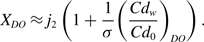 \begin{align}{X_{DO}} \approx {j_2}\left( {1 + \frac{1}{\sigma }{{\left( {\frac{{C{d_w}}}{{C{d_0}}}} \right)}_{DO}}} \right).\end{align}
This is also approximately independent of $\delta$
DO
, with a 10% error in (Cd
w
)
DO
changing X
DO
by only about 1%. The optimum Mach number is given by
$\delta$
DO
, with a 10% error in (Cd
w
)
DO
changing X
DO
by only about 1%. The optimum Mach number is given by
 \begin{align}{M_{DO}} = \left( {\frac{{{{\left( {{M_{CC}}} \right)}_{DO}}}}{{cos\!\left( {{{\rm{\Lambda }}_w}} \right)}}} \right){X_{DO}} \approx {j_2}\left( {1 + \frac{1}{\sigma }{{\left( {\frac{{C{d_w}}}{{C{d_0}}}} \right)}_{DO}}} \right)\left( {\frac{{{{\left( {{M_{CC}}} \right)}_{DO}}}}{{cos\!\left( {{{\rm{\Lambda }}_w}} \right)}}} \right),\end{align}
but, since $M_{DO}$
is proportional to
$M_{DO}$
is proportional to $(M_{cc})_{DO}$
, estimates for
$(M_{cc})_{DO}$
, estimates for $M_{DO}$
are subject to at least the same uncertainty as
$M_{DO}$
are subject to at least the same uncertainty as $(M_{cc})_{DO}$
, i.e.
$(M_{cc})_{DO}$
, i.e. $\pm$
7%. This is not accurate enough for practical applications. However, using public domain sources, Poll and Schumann [Reference Poll3] have obtained estimates for
$\pm$
7%. This is not accurate enough for practical applications. However, using public domain sources, Poll and Schumann [Reference Poll3] have obtained estimates for $M_{DO}$
, whose maximum error is about
$M_{DO}$
, whose maximum error is about $\pm$
4% and better than
$\pm$
4% and better than $\pm$
2% in most of the cases considered. Therefore, since more accurate values are already available, the lack of accuracy associated with Equation (46) does not present an insurmountable problem and
$\pm$
2% in most of the cases considered. Therefore, since more accurate values are already available, the lack of accuracy associated with Equation (46) does not present an insurmountable problem and $M_{DO}$
can be treated as an input rather than an output.
$M_{DO}$
can be treated as an input rather than an output.
In addition, from Equations (40) and (45),
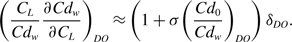 \begin{align}{\left( {\frac{{{C_L}}}{{C{d_w}}}\frac{{\partial C{d_w}}}{{\partial {C_L}}}} \right)_{DO}} \approx \left( {1 + \sigma {{\left( {\frac{{C{d_0}}}{{C{d_w}}}} \right)}_{DO}}} \right){\delta _{DO}}.\end{align}
Hence, from Equations (24) and (25),
 \begin{align}{\left( {{C_L}} \right)_{DO}} \approx \left( {1 - {1 \over 2}\left( {b\!\left( {1 + \left( {{{{k_1}} \over K}} \right)} \right)\left( {1 + {{\rm{\Gamma }}_{DO}}} \right) + \sigma {\delta _{DO}} - \left( {1 - {\delta _{DO}}} \right){{\left( {{{C{d_w}} \over {C{d_0}}}} \right)}_{DO}}} \right)} \right)\left( {{{C{d_0}} \over K}} \right)_{DO}^{1/2}\end{align}
and
 \begin{align}{\left( {Cd} \right)_{DO}} \approx 2\left( {1 - \frac{1}{2}\left( {b\!\left( {1 + \left( {\frac{{{k_1}}}{K}} \right)} \right)\left( {1 + {{\rm{\Gamma }}_{DO}}} \right) + \sigma {\delta _{DO}} - \left( {2 - {\delta _{DO}}} \right){{\left( {\frac{{C{d_w}}}{{C{d_0}}}} \right)}_{DO}}} \right)} \right){\left( {C{d_0}} \right)_{DO}}.\end{align}
Both these relations involve $\delta$
DO
, which is a function of (C
L
)
DO
and the coefficients in Equation (34). However, it is easily shown that both (C
L
)
DO
and (Cd)
DO
are also relatively insensitive to
$\delta$
DO
, which is a function of (C
L
)
DO
and the coefficients in Equation (34). However, it is easily shown that both (C
L
)
DO
and (Cd)
DO
are also relatively insensitive to $\delta$
DO
, with a 10% error resulting in a change of less than 0.5% in either quantity, whilst a 10% error in (Cd
w
)
DO
only changes (C
L
)
DO
by about 0.25% and (Cd)
DO
by 0.5%. Therefore, using mid-range values and taking j
1
and j
2
to be 0.080 and 0.875, respectively,
$\delta$
DO
, with a 10% error resulting in a change of less than 0.5% in either quantity, whilst a 10% error in (Cd
w
)
DO
only changes (C
L
)
DO
by about 0.25% and (Cd)
DO
by 0.5%. Therefore, using mid-range values and taking j
1
and j
2
to be 0.080 and 0.875, respectively,
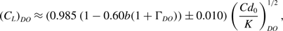 \begin{align}{\left( {{C_{}}} \right)_{DO}} \approx \left( {0.985\left( {1 - 0.60b\!\left( {1 + {{\rm{\Gamma }}_{DO}}} \right)} \right) \pm 0.010} \right)\left( {{{C{d_0}} \over K}} \right)_{DO}^{1/2},\end{align}
 \begin{align}{\left( {Cd} \right)_{DO}} \approx 2\!\left( {1.035\left( {1 - 0.68b\!\left( {1 + {{\rm{\Gamma }}_{DO}}} \right)} \right){\rm{\;}} \pm 0.025{\rm{\;}}} \right){\left( {C{d_0}} \right)_{DO}}\end{align}
and
 \begin{align}{\left( {{L \over D}} \right)_{DO}} \approx {1 \over 2}\left( {0.950\left( {1 + 0.08b\!\left( {1 + {{\rm{\Gamma }}_{DO}}} \right)} \right){\rm{\;}} \pm 0.025{\rm{\;}}} \right)\left( {{1 \over {KC{d_0}}}} \right)_{DO}^{1/2}.\end{align}
These “first-order” estimates are very simple, yet surprisingly accurate, and they reveal the fundamental character of the solution.
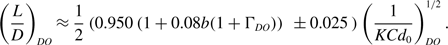
Using (C L ) DO from Equation (50), together with Equations (34) and (41), gives
 \begin{align} \delta_{DO} \approx \frac{0.266}{\cos^{2}\left( \Lambda_{w} \right)}\left( 1 + \frac{0.133}{\cos^{2}\left( \Lambda_{w} \right)}\left( 1 - 0.60b\!\left( 1 + \Gamma_{DO} \right) \right)\left( \frac{{Cd}_{0}}{K} \right)_{DO}^{\frac{1}{2}} \right) \times \nonumber & \\\left( {\left( {1 - 0.60b\!\left( {1 + {{\rm{\Gamma }}_{DO}}} \right)} \right)\left( {{{C{d_0}} \over K}} \right)_{DO}^{1/2}} \right)&.\end{align}
Substituting this result into Equations (48) and (49) gives accurate estimates for (C
L
)
DO
and (C
d
)
DO
that depend upon known aircraft geometric parameters and engine characteristics, plus (Cd
0
)
DO
, which in turn depends upon the, yet to be determined, Reynolds number, $R_{DO}^{ac}$
.
$R_{DO}^{ac}$
.
At this stage, the presentation can be simplified by adopting the “ $\psi$
” notation originally introduced by Poll and Schumann [2, Reference Poll3]. Therefore, at the design optimum condition,
$\psi$
” notation originally introduced by Poll and Schumann [2, Reference Poll3]. Therefore, at the design optimum condition,
 \begin{align}{M_{DO}} = {\psi _4}\end{align}
and, using equation (A-6) from Appendix A, the Reynolds number may be written as
 \begin{align}R_{DO}^{ac} = {{{\psi _5}} \over {\left( {1 + 1.34{{\left( {\overline {\Delta T} } \right)}_{DO}}} \right)}}{\left( {{{{{\left( {{p_\infty }} \right)}_{DO}}} \over {{{\left( {{p_{TP}}} \right)}_{ISA}}}}} \right)^{{\iota _{DO}}}},\end{align}
where
 \begin{align}{\psi _5} = {\left( {\frac{{S_{ref}^{1/2}{\psi _4}\gamma {p_{TP}}}}{{{\mu _{TP}}{a_{TP}}}}} \right)_{ISA}}.\end{align}
Whilst, from the definition of lift coefficient,
 \begin{align}{\left( {{C_L}} \right)_{DO}} = {\psi _6}\left( {{m \over {MTOM}}} \right)\left( {{{{{\left( {{p_{TP}}} \right)}_{ISA}}} \over {{{\left( {{p_\infty }} \right)}_{DO}}}}} \right) = {\psi _6}\left( {{m \over {MTOM}}} \right){\left( {{{{\psi _5}} \over {\left( {1 + 1.34{{\left( {\overline {\Delta T} } \right)}_{DO}}} \right)R_{DO}^{ac}}}} \right)^{{1 \over {{\iota _{DO}}}}}},\end{align}
with
 \begin{align}{\psi _6} = \left( {\frac{{MTOM.g}}{{\left( {\gamma /2} \right){{\left( {{p_{TP}}} \right)}_{ISA}}\psi _4^2{S_{ref}}}}} \right).\end{align}
where MTOM is the aircraft’s maximum permitted take-off mass. Also following Poll and Schumann [2] and as described in Appendix B, the variation of e
LS
with $C_F^{ac}$
may be approximated by a power law of the form
$C_F^{ac}$
may be approximated by a power law of the form
 \begin{align}{e_{LS}} \approx \frac{E}{{{{\left( {C_F^{ac}} \right)}^\tau }}}.\end{align}
However, in contrast to Poll and Schumann [2] and following Equation (50), the definition of $\Psi$
2 is changed (slightly) from the original version to read
$\Psi$
2 is changed (slightly) from the original version to read
 \begin{align}{\psi _2} = \frac{{{{\left( {{C_L}} \right)}_{DO}}}}{{\left( {1 - 0.60b\!\left( {1 + {{\rm{\Gamma }}_{DO}}} \right)} \right)}}\left( {\frac{1}{{C_F^{ac}}}} \right)_{DO}^{\left( {\frac{{1 - \tau }}{2}} \right)}.\end{align}
Combining Equations (55), (57) and (60), the value of the mass ratio at which the design cruise coincides with the 226.32 hPa isobar, i.e. (p ∞ ) DO equals (p TP ) ISA , is
 \begin{align}{\left( {{m \over {MTOM}}} \right)_{{{\left( {{p_{TP}}} \right)}_{ISA}}}} \approx \left( {1 + {b \over 2}\left( {1.34\left( {1 - \tau } \right){{\left( {\overline {\Delta T} } \right)}_{DO}} - 1.20\left( {1 + {{\rm{\Gamma }}_{DO}}} \right)} \right)} \right){\psi _7},\end{align}
where
 \begin{align}{\psi _7} = \frac{{{\psi _2}}}{{{\psi _6}}}{\left( {\frac{a}{{\psi _5^b}}} \right)^{\left( {\frac{{1 - \tau }}{2}} \right)}}.\end{align}
This simple result, which only depends upon input parameters, determines the value of $\iota$
DO
, since, when the mass ratio exceeds this value, (p
∞
)
DO
is more than 226.32 hPa and
$\iota$
DO
, since, when the mass ratio exceeds this value, (p
∞
)
DO
is more than 226.32 hPa and $\iota$
DO
is 0.74505. Conversely, if the mass ratio is less than, or equal to, this value, (p
∞
)
DO
is less than 226.32 hPa and
$\iota$
DO
is 0.74505. Conversely, if the mass ratio is less than, or equal to, this value, (p
∞
)
DO
is less than 226.32 hPa and $\iota$
DO
is equal to one.
$\iota$
DO
is equal to one.
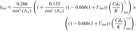
The Reynolds number at the design condition is then found by combining Equations (57) and (60), eliminating (C L ) DO to give,
 \begin{align}R_{DO}^{ac} \approx {{{\psi _5}} \over {\left( {1 + {\kappa _{DO}}\left( {1.34{{\left( {\overline {\Delta T} } \right)}_{DO}} - 0.60{\iota _O}b\!\left( {1 + {{\rm{\Gamma }}_{DO}}} \right)} \right)} \right)}}{\left( {{1 \over {{\psi _7}}}\left( {{m \over {MTOM}}} \right)} \right)^{{\iota _{DO}}{\kappa _{DO}}}},\end{align}
where
 \begin{align}{\kappa _{DO}} = \left( {\frac{2}{{2 - {\iota _{DO}}b\!\left( {1 - \tau } \right)}}} \right).\end{align}
Therefore, for a given aircraft weight, m, the design Reynolds number depends upon fixed aircraft characteristics and the design atmospheric parameters all of which are known.
Having obtained the Reynolds number, the skin friction coefficient is given by
 \begin{align}{\left( {C_F^{ac}} \right)_{DO}} \approx \left( {1 + {\kappa _{DO}}b\!\left( {1.34{{\left( {\overline {\Delta T} } \right)}_{DO}} - 0.60{\iota _{DO}}b\!\left( {1 + {{\rm{\Gamma }}_{DO}}} \right)} \right)} \right)\left( {{a \over {\psi _5^b}}} \right){\left( {{\psi _7}\left( {{{MTOM} \over m}} \right)} \right)^{{\iota _{DO}}{\kappa _{DO}}b}}.\end{align}
Since the Reynolds number is being raised to a power lying in the range 0.1 to 0.15, the use of Equation (50) to give (C
L
)
DO
introduces an error in ${\left( {C_F^{ac}} \right)_{DO}}$
of less than 0.25%. Hence, an accurate approximate solution for (Cd
0
)
DO
is obtained by using Equations (16) and (65) and values of (Cd
w
)
DO
and
${\left( {C_F^{ac}} \right)_{DO}}$
of less than 0.25%. Hence, an accurate approximate solution for (Cd
0
)
DO
is obtained by using Equations (16) and (65) and values of (Cd
w
)
DO
and $\delta$
DO
follow from Equations (43) and (53). Equations (46), (48) and (49) yield estimates for M
DO
, (C
L
)
DO
and (Cd)
DO
and, using Equations (26) and (52),
$\delta$
DO
follow from Equations (43) and (53). Equations (46), (48) and (49) yield estimates for M
DO
, (C
L
)
DO
and (Cd)
DO
and, using Equations (26) and (52),
 \begin{align}{\left( {{L \over D}} \right)_{DO}} \approx {1 \over 2}\left( {1 - {1 \over 2}{{\left( {{{C{d_w}} \over {C{d_0}}}} \right)}_{DO}}} \right)\left( {{1 \over {KC{d_0}}}} \right)_{DO}^{1/2} \approx \left( {1 + 0.08b\!\left( {1 + {{\rm{\Gamma }}_{DO}}} \right)} \right){\psi _3}\left( {{1 \over {C_F^{ac}}}} \right)_{DO}^{\left( {{{1 + \tau } \over 2}} \right)}.\end{align}
Finally, using Equations (11) and (66), the design value of ( $\eta$
o
L/D) is given by
$\eta$
o
L/D) is given by
 \begin{align}{\left( {{\eta _o}L/D} \right)_{DO}} \approx \left( {{\eta _1}{{\left( {{M_{DO}}} \right)}^{{\eta _2}}}} \right){\left( {\frac{L}{D}} \right)_{DO}} = \left( {1 + 0.08b\!\left( {1 + {{\rm{\Gamma }}_{DO}}} \right)} \right){\psi _1}\left( {\frac{1}{{C_F^{ac}}}} \right)_{DO}^{\left( {\frac{{1 + \tau }}{2}} \right)}\end{align}
and, hence,
 \begin{align}{\left( {{\eta _o}} \right)_{DO}} = \frac{{{\psi _1}}}{{{\psi _3}}}\;.\end{align}
This completes the approximate solution for the design optimum condition.
7.0 Evaluating the characteristics at the design optimum
Although the actual design optimum conditions are known only to the aircraft manufacturer, for illustrative purposes, it is assumed that they correspond to operation in the ISA with the aircraft at 80% of its maximum permitted take-off mass, MTOM. This being the case, the input parameters are MTOM, the wing reference area, S
ref
, span, s, quarter chord sweep angle, $\Lambda$
w
, and whether, or not, winglets are fitted, the fuselage maximum width, b
f
, plus the nominal bypass ratio, BPR, together with estimates for the zero-lift drag parameter,
$\Lambda$
w
, and whether, or not, winglets are fitted, the fuselage maximum width, b
f
, plus the nominal bypass ratio, BPR, together with estimates for the zero-lift drag parameter, $\Psi$
0 (Equation 16), M
DO
, and (
$\Psi$
0 (Equation 16), M
DO
, and ( $\eta$
o
L/D)
DO
. As described in Poll and Schumann [Reference Poll3],
$\eta$
o
L/D)
DO
. As described in Poll and Schumann [Reference Poll3], $\Psi$
0 is determined solely by the airframe geometry, which is relatively easy to find, whilst the most difficult parameters to estimate are M
DO
and (
$\Psi$
0 is determined solely by the airframe geometry, which is relatively easy to find, whilst the most difficult parameters to estimate are M
DO
and ( $\eta$
o
L/D)
DO
. However, methods for obtaining these quantities from public domain sources are described in Poll and Schumann [Reference Poll3], which also contains complete data sets for 53 aircraft and engine combinations. In terms of the
$\eta$
o
L/D)
DO
. However, methods for obtaining these quantities from public domain sources are described in Poll and Schumann [Reference Poll3], which also contains complete data sets for 53 aircraft and engine combinations. In terms of the $\Psi$
parameters,
$\Psi$
parameters, $\Psi$
1 is obtained from (
$\Psi$
1 is obtained from ( $\eta$
o
L/D)
DO
(Equation (67)),
$\eta$
o
L/D)
DO
(Equation (67)), $\Psi$
4 is equal to M
DO
(Equation (54)),
$\Psi$
4 is equal to M
DO
(Equation (54)), $\Psi$
5 depends upon S
ref
and
$\Psi$
5 depends upon S
ref
and $\Psi$
4 (Equation (57)),
$\Psi$
4 (Equation (57)), $\Psi$
6 depends upon MTOM, S
ref
and
$\Psi$
6 depends upon MTOM, S
ref
and $\Psi$
4 (Equation (58)), i.e. they depend only upon the input parameters, whilst
$\Psi$
4 (Equation (58)), i.e. they depend only upon the input parameters, whilst $\Psi$
2,
$\Psi$
2, $\Psi$
3 and
$\Psi$
3 and $\Psi$
7 are outputs. Since the various quantities at the design optimum conditions for a given aircraft only need to be computed once, in order to have accurate and self-consistent values, Equation (42) has been used to link (C
L
)
DO
to
$\Psi$
7 are outputs. Since the various quantities at the design optimum conditions for a given aircraft only need to be computed once, in order to have accurate and self-consistent values, Equation (42) has been used to link (C
L
)
DO
to $\delta$
DO
and solutions obtained by iteration.
$\delta$
DO
and solutions obtained by iteration.
The original data base was published some three years ago and, since that time, the values have been reviewed, refined and improved. This has resulted in some minor amendments and extensions being made and latest updated values are presented here.
As already noted, the calculation requires a knowledge of $\Psi$
0
. In Poll and Schumann [Reference Poll3] this parameter was obtained from information given Fig. 40.17 of Obert [Reference Obert15] and, as indicted in Fig. 1 of Ref. [Reference Poll and Schumann5], these values are subject to an uncertainty of more than ±10%. However, Chapter 24 of the same reference contains additional information on the variation of drag with Mach number at fixed values of the lift coefficient for 11 of the aircraft types in the PS data base. These types are marked with an “*” in Table 1. In all, there are 31 values for the drag coefficient at a Mach number of about 0.5 for values of C
L
between 0.3 and 0.5 and all lie within the expected range of validity of Equation (15). Since Equation (23) is well established, this was used to determine K, whilst
$\Psi$
0
. In Poll and Schumann [Reference Poll3] this parameter was obtained from information given Fig. 40.17 of Obert [Reference Obert15] and, as indicted in Fig. 1 of Ref. [Reference Poll and Schumann5], these values are subject to an uncertainty of more than ±10%. However, Chapter 24 of the same reference contains additional information on the variation of drag with Mach number at fixed values of the lift coefficient for 11 of the aircraft types in the PS data base. These types are marked with an “*” in Table 1. In all, there are 31 values for the drag coefficient at a Mach number of about 0.5 for values of C
L
between 0.3 and 0.5 and all lie within the expected range of validity of Equation (15). Since Equation (23) is well established, this was used to determine K, whilst $\Psi$
0
was varied until the values for Cd given by Equation (16) were brought into best alignment with the Obert value for each aircraft. The resulting data set had an RMS deviation of about 1% and a maximum deviation of less than 2.5%. Ratios of the new
$\Psi$
0
was varied until the values for Cd given by Equation (16) were brought into best alignment with the Obert value for each aircraft. The resulting data set had an RMS deviation of about 1% and a maximum deviation of less than 2.5%. Ratios of the new $\Psi$
0
to the original values were then plotted against the date of the aircraft’s first flight and the result is given in Fig. 5.
$\Psi$
0
to the original values were then plotted against the date of the aircraft’s first flight and the result is given in Fig. 5.
Updated input data for a range of turbofan powered, civil transport aircraft. The “*” indicates that additional drag data is available in Obert [Reference Obert15]
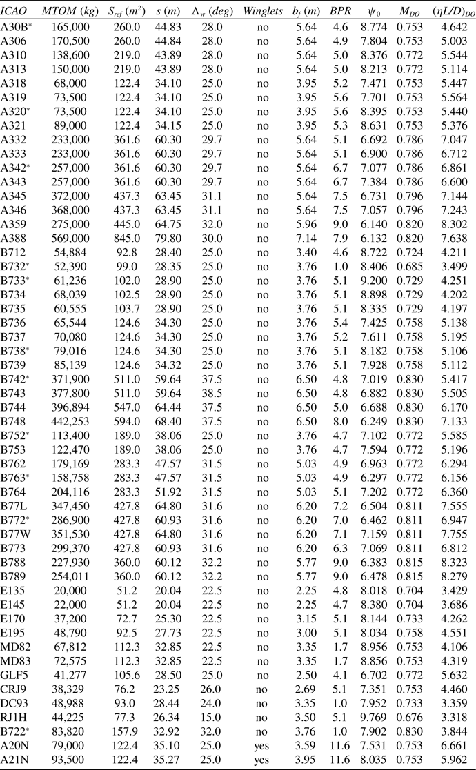
The variation of the $\Psi$
0
correction factor based upon data from Obert [Reference Obert15] with the date of the aircraft’s first flight.
$\Psi$
0
correction factor based upon data from Obert [Reference Obert15] with the date of the aircraft’s first flight.
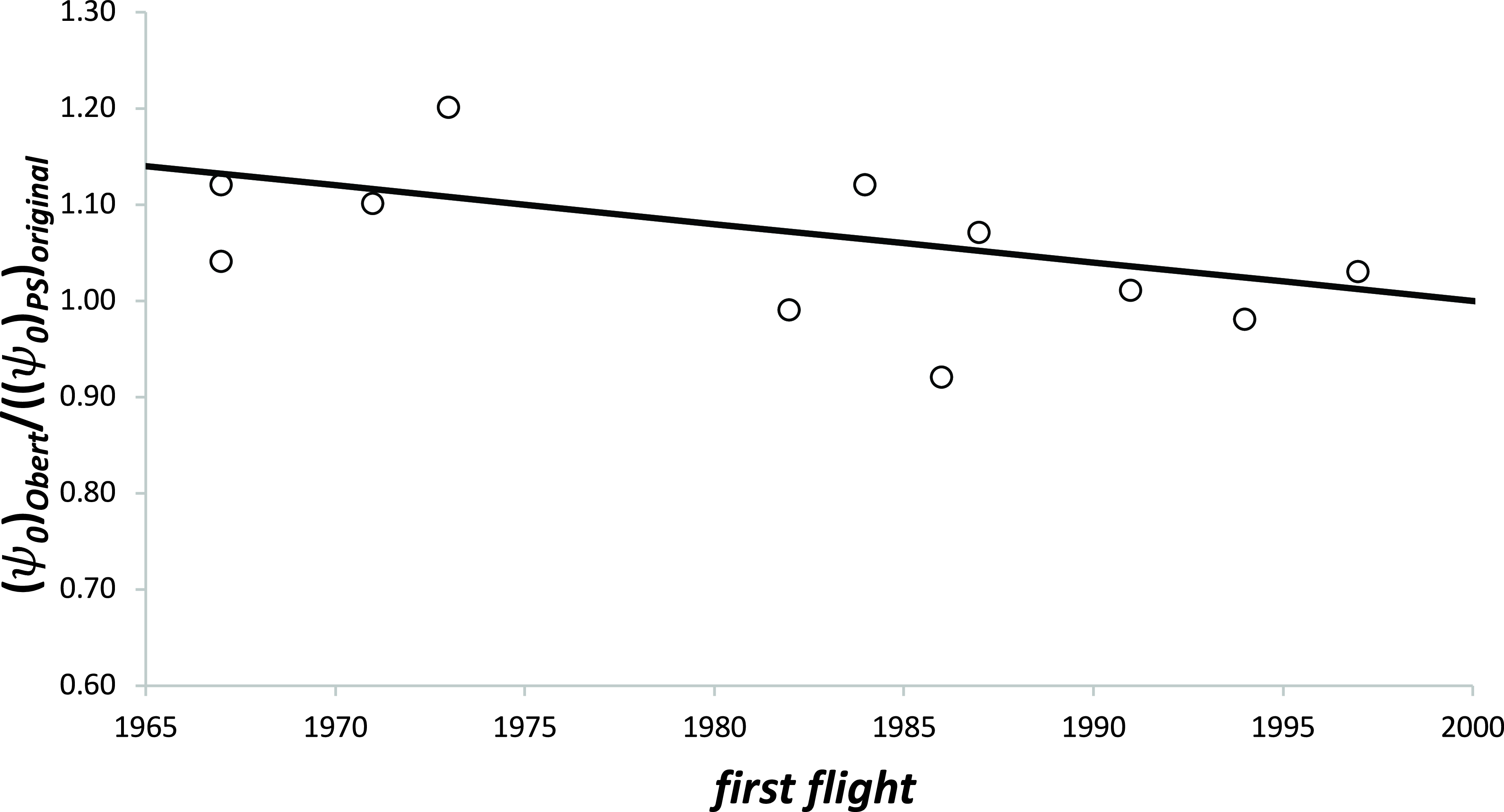
Whilst the scatter is still about ±10 %, the data indicate that, for a given aircraft geometry, $\Psi$
0
and, hence, (Cd
0
)
DO
, has been reducing steadily over time. Although not identified in Ref. (Reference Poll and Schumann5), this trend is to be expected, since improved aerodynamic design has reduced the interference effects between the various components, including that between the wing and the engines, and improved manufacturing techniques have reduced excrescence drag and surface roughness. These new results suggest that, between 1970 and 2000,
$\Psi$
0
and, hence, (Cd
0
)
DO
, has been reducing steadily over time. Although not identified in Ref. (Reference Poll and Schumann5), this trend is to be expected, since improved aerodynamic design has reduced the interference effects between the various components, including that between the wing and the engines, and improved manufacturing techniques have reduced excrescence drag and surface roughness. These new results suggest that, between 1970 and 2000, $\Psi$
0
has decreased by about 15% and a “best fit” gives
$\Psi$
0
has decreased by about 15% and a “best fit” gives
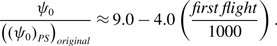 \begin{align}\;\frac{{{\psi _0}}}{{{{\left( {{{\left( {{\psi _0}} \right)}_{PS}}} \right)}_{original}}}} \approx 9.0 - 4.0\left( {\frac{{first\;flight}}{{1000}}} \right).\end{align}
Hence, a small, but significant, improvement to the overall accuracy of the method can be achieved by applying a simple correction factor to the original values of $\Psi$
0
. Where the factor for a particular aircraft type is given by Obert, the Obert value is used. In all other cases, an estimate is obtained from Equation (69).
$\Psi$
0
. Where the factor for a particular aircraft type is given by Obert, the Obert value is used. In all other cases, an estimate is obtained from Equation (69).
In Ref. (Reference Poll3), nominal values for bypass ratio were provided for specific engines. However, most aircraft can be fitted with more than one engine type and, in some instances, the precise engine type may not be known. Therefore, to cover the more general case, the average BPR for all engine types fitted to each aircraft type was obtained using the data provided in the ICAO engine data base [17]. These values were used to estimate $\eta$
2 via Equation (36) from Poll and Schumann [Reference Poll3]. The revised input values are given in Table 1.
$\eta$
2 via Equation (36) from Poll and Schumann [Reference Poll3]. The revised input values are given in Table 1.
The parameters $\Psi$
4
,
$\Psi$
4
, $\Psi$
5 and
$\Psi$
5 and $\Psi$
6 retain the values given in Poll and Schumann [Reference Poll3]. However, since their definitions have changed, the parameters
$\Psi$
6 retain the values given in Poll and Schumann [Reference Poll3]. However, since their definitions have changed, the parameters $\tau$
,
$\tau$
, $\Psi$
1
,
$\Psi$
1
, $\Psi$
2,
$\Psi$
2, $\Psi$
3 and
$\Psi$
3 and $\Psi$
7 must be recomputed.
$\Psi$
7 must be recomputed.
The procedure began by obtaining initial estimates for $\tau$
and E using Equations (C-4) and (C-5) from Appendix C and giving (Cd
0
)
DO
the mid-range value of 0.0175. An initial estimate for
$\tau$
and E using Equations (C-4) and (C-5) from Appendix C and giving (Cd
0
)
DO
the mid-range value of 0.0175. An initial estimate for $\Psi$
2
was obtained by combining Equations (16), (18), (50), (59) and (60) to give
$\Psi$
2
was obtained by combining Equations (16), (18), (50), (59) and (60) to give
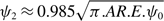 \begin{align}{\psi _2} \approx 0.985\sqrt {\pi .AR.E.{\psi _0}} \end{align}
and an estimate for $\psi_{7}$
was then obtained from Equation (62). If the assumed value of (m/MTOM) was less than, or equal to,
$\psi_{7}$
was then obtained from Equation (62). If the assumed value of (m/MTOM) was less than, or equal to, $\psi_{7}$
, the static pressure at cruise,
$\psi_{7}$
, the static pressure at cruise, $(p_{\infty})_{DO}$
, must be less than 226.32 hPa and
$(p_{\infty})_{DO}$
, must be less than 226.32 hPa and $\iota_{DO}$
was set to unity, otherwise
$\iota_{DO}$
was set to unity, otherwise $\iota_{DO}$
was set to 0.74505. Furthermore, since the aircraft is operating in the ISA,
$\iota_{DO}$
was set to 0.74505. Furthermore, since the aircraft is operating in the ISA, $\Gamma_{DO}$
is zero when
$\Gamma_{DO}$
is zero when $\iota_{DO}$
is unity, otherwise it is equal to −0.255. The initial estimate for
$\iota_{DO}$
is unity, otherwise it is equal to −0.255. The initial estimate for $R_{DO}^{ac}$
found from Equation (63), followed by
$R_{DO}^{ac}$
found from Equation (63), followed by $\left( C_{F}^{ac} \right)_{DO}$
and
$\left( C_{F}^{ac} \right)_{DO}$
and $(CD_{0})_{DO}$
from Equations (16) and (17). The parameters
$(CD_{0})_{DO}$
from Equations (16) and (17). The parameters $(k_{1})_{DO}$
and
$(k_{1})_{DO}$
and $(k)_{DO}$
follow from Equations (22) and (23). Taking
$(k)_{DO}$
follow from Equations (22) and (23). Taking $j_{1}$
and
$j_{1}$
and $j_{2}$
to be 0.080 and 0.875, respectively, Equations (43) and (45) were then used to obtain (
$j_{2}$
to be 0.080 and 0.875, respectively, Equations (43) and (45) were then used to obtain ( $Cd_{w}$
/
$Cd_{w}$
/ $Cd_{0})_{DO}$
and
$Cd_{0})_{DO}$
and $X_{DO}$
. Since
$X_{DO}$
. Since $M_{DO}$
is assumed to be equal to the value of
$M_{DO}$
is assumed to be equal to the value of $\psi_{DO}$
given in Poll and Schumann [Reference Poll3], from Equation (31)
$\psi_{DO}$
given in Poll and Schumann [Reference Poll3], from Equation (31)
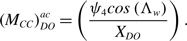 \begin{align}\left( {{M_{CC}}} \right)_{DO}^{ac} = \left( {\frac{{{\psi _4}cos\left( {{{\rm{\Lambda }}_w}} \right)}}{{{X_{DO}}}}} \right).\end{align}
This was combined with (C
L
)
DO
from Equation (60) to give $\delta$
DO
from Equation (41). In addition, this allows the estimation of a self-consistent value of the overall wing technology factor,
$\delta$
DO
from Equation (41). In addition, this allows the estimation of a self-consistent value of the overall wing technology factor, ${\left( {{M_{TF}}} \right)^{ac}}$
, to be obtained from Equation (34), i.e.
${\left( {{M_{TF}}} \right)^{ac}}$
, to be obtained from Equation (34), i.e.
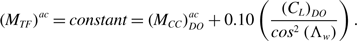 \begin{align}{\left( {{M_{TF}}} \right)^{ac}} = constant = \left( {{M_{CC}}} \right)_{DO}^{ac} + 0.10\left( {\frac{{{{\left( {{C_L}} \right)}_{DO}}}}{{co{s^2}\left( {{\Lambda _w}} \right)}}} \right).\end{align}
At this point, the values of (Cd
w
/Cd
0
)
DO
, $\delta$
DO
,
$\delta$
DO
, $\iota$
DO
and
$\iota$
DO
and $\eta$
2 were used to obtain an improved estimate for (C
L
)
DO
from Equation (42). The value of (p
∞
)
DO
was then obtained from the definition of lift coefficient (Equation (5)). This was then used in Equation (55) to give a new value of
$\eta$
2 were used to obtain an improved estimate for (C
L
)
DO
from Equation (42). The value of (p
∞
)
DO
was then obtained from the definition of lift coefficient (Equation (5)). This was then used in Equation (55) to give a new value of $R_{DO}^{ac}$
and in Equations (D-1) or (D-2) from Appendix D to give the corresponding flight level, (FL)
DO
. The revised values of (C
L
)
DO
and
$R_{DO}^{ac}$
and in Equations (D-1) or (D-2) from Appendix D to give the corresponding flight level, (FL)
DO
. The revised values of (C
L
)
DO
and $R_{DO}^{ac}$
were then used as input and the process repeated until full convergence was achieved. Corresponding values of
$R_{DO}^{ac}$
were then used as input and the process repeated until full convergence was achieved. Corresponding values of $\tau$
, E,
$\tau$
, E, $\Psi$
2
and
$\Psi$
2
and $\Psi$
7
were then obtained. It was found that the difference between the fully converged results and the initial estimates from the approximate solution was less than 2.5% for all parameters.
$\Psi$
7
were then obtained. It was found that the difference between the fully converged results and the initial estimates from the approximate solution was less than 2.5% for all parameters.
Finally, in Poll and Schumann [Reference Poll3] the values of $\Psi$
1
were obtained by calibration using public domain information for (
$\Psi$
1
were obtained by calibration using public domain information for ( $\eta$
o
L/D). Therefore, since the definition of
$\eta$
o
L/D). Therefore, since the definition of $\tau$
has changed,
$\tau$
has changed, $\Psi$
1
must also be recalculated to match these original values. The full set of results is given in Tables 2 and 3.
$\Psi$
1
must also be recalculated to match these original values. The full set of results is given in Tables 2 and 3.
Estimates of the performance characteristics at the design condition (aircraft operating in the ISA with a mass of 80% MTOM)
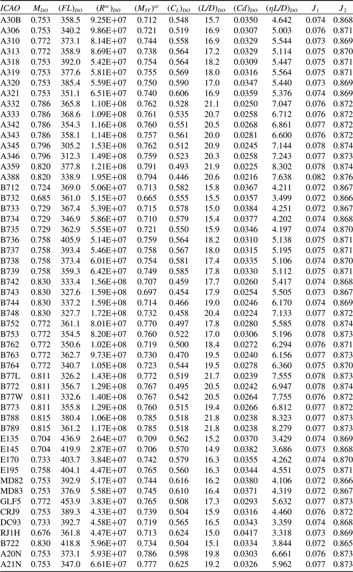
Revised estimates of the PS characteristic parameters
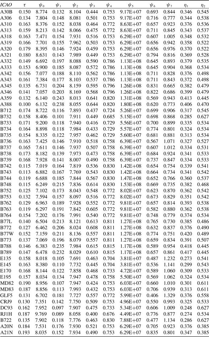
8.0 A Modified wave drag model
Shevell [Reference Shevell8] assumes that there is a unique relationship between Cd w and X, but, in practice, this is unlikely to be the case. However, since it is being assumed that the value of M DO is known, Shevell’s concept can be used to construct a “bespoke” wave drag model for each aircraft that has the correct behaviour at the design optimum condition.
The general expression for X is obtained by combining Equations (31), (34) and (71), i.e.
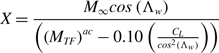 \begin{align}X = \frac{{{M_\infty }cos\left( {{\Lambda _w}} \right)}}{{\left( {{{\left( {{M_{TF}}} \right)}^{ac}} - 0.10\left( {\frac{{{C_L}}}{{co{s^2}\left( {{\Lambda _w}} \right)}}} \right)} \right)}}\end{align}
and, in the immediate vicinity of the design optimum condition, let the wave drag can be represented by a generalised form of equation (38), i.e.
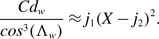 \begin{align}\frac{{C{d_w}}}{{co{s^3}\!\left( {{{\rm{\Lambda }}_w}} \right)}} \approx {j_1}{\left( {X - {j_2}} \right)^2}.\end{align}
Therefore, at the design optimum condition, combining this with Equation (40) gives
 \begin{align}{j_1} = \left( {\frac{1}{{\delta .X}}} \right)_{DO}^2\left( {\frac{{{C_L}}}{{C{d_0}}}\frac{{\partial C{d_w}}}{{\partial {C_L}}}} \right)_{DO}^2{\left( {\frac{{C{d_0}}}{{C{d_w}}}} \right)_{DO}}\left( {\frac{{{{\left( {C{d_0}} \right)}_{DO}}}}{{co{s^3}\!\left( {{\Lambda _w}} \right)}}} \right)\end{align}
and, hence,
 \begin{align}{j_2} = {X_{DO}} - \sqrt {\frac{1}{{{j_1}}}{{\left( {\frac{{C{d_w}}}{{C{d_0}}}} \right)}_{DO}}\left( {\frac{{{{\left( {C{d_0}} \right)}_{DO}}}}{{co{s^3}\!\left( {{\Lambda _w}} \right)}}} \right)}.\end{align}
If it is assumed that the Cd w at the design condition is given by Equation (43), the corresponding lift coefficient can be found by iterative solution of Equation (42), using the approximate result given in Equation (50) as the first guess. This guarantees that all the conditions for the design optimum are met and the numerical values are self-consistent.
Using Equation (A-16) from Appendix A, the revised coefficients J 1 and J 2 are
 \begin{align}{j_1} = \frac{1}{{16.3}}\left( {\frac{{\left( {1 - b\!\left( {1 + {\rm{\Gamma }}} \right)} \right) + 16.3{\sigma ^2}\frac{{C{d_0}}}{{co{s^3}\!\left( {{{\rm{\Lambda }}_w}} \right)}} - \left( {1 + \left( {\frac{{{k_1}}}{K}} \right)b\!\left( {1 + {{\rm{\Gamma }}_{DO}}} \right)} \right)\left( {\frac{{KC_L^2}}{{C{d_0}}}} \right)}}{{\sigma \delta X}}} \right)_{DO}^2\end{align}
and
 \begin{align}{j_2} = {X_{DO}} - \sqrt {\frac{{16.3}}{{{j_1}}}} \left( {\sigma \frac{{{{\left( {C{d_0}} \right)}_{DO}}}}{{co{s^3}\!\left( {{\Lambda _w}} \right)}}} \right).\end{align}
Since J 1 and J 2 depend only upon aircraft and engine characteristics, these parameters are also characteristics of the aircraft-engine combination. Hence, J 1 and J 2 are included in Table 3.
For values of X greater than X DO , an additional term is required to capture the drag generated by strong shock waves. At this stage in the development of the model, it is proposed that the additional wave drag as X increases be represented by a variant of Equation (37), i.e.
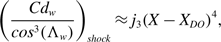 \begin{align}{\left( {\frac{{C{d_w}}}{{co{s^3}\!\left( {{{\rm{\Lambda }}_w}} \right)}}} \right)_{shock}} \approx {j_3}{\left( {X - {X_{DO}}} \right)^4},\end{align}
where $j_{3}$
is a constant that needs to be determined by calibration. However, initial indications are that
$j_{3}$
is a constant that needs to be determined by calibration. However, initial indications are that $j_{3}$
is of order 100. Hence, for values of X greater than X
DO
, the wave drag coefficient is given by
$j_{3}$
is of order 100. Hence, for values of X greater than X
DO
, the wave drag coefficient is given by
 \begin{align}{\left( {C{d_w}} \right)_{rise}} \approx co{s^3}\!\left( {{{\rm{\Lambda }}_w}} \right)\left( {{j_1}{{\left( {X - {j_2}} \right)}^2} + {j_3}{{\left( {X - {X_{DO}}} \right)}^4}} \right).\end{align}
This revised model allows the aircraft’s lift-to-drag ratio to be estimated for any combination of Mach number and lift coefficient.
9.0 Updating the ps method
As described in Poll and Schumann [2, Reference Poll3], application of the PS method for the estimation of the cruise values of ( $\eta$
o
L/D) for any combination of mass, Mach number and flight levelFootnote
7
requires a knowledge of the operational optimum conditions for (
$\eta$
o
L/D) for any combination of mass, Mach number and flight levelFootnote
7
requires a knowledge of the operational optimum conditions for ( $\eta$
o
L/D) for the actual mass and the specific atmosphere being encountered. The operational optima are governed by Equations (8) and (9), whilst the design optimum is governed by Equations (13) and (14), and so, in general, the two conditions will not be the same. Whilst the full model described in the previous sections can always be used to determine the operational optimum, this will need to be done numerically. However, in practise, the differences between the design optimum and the operational optima are expected to be small and so, to a good approximation, operational optimum conditions may be expressed as perturbations of the design optimum values.
$\eta$
o
L/D) for the actual mass and the specific atmosphere being encountered. The operational optima are governed by Equations (8) and (9), whilst the design optimum is governed by Equations (13) and (14), and so, in general, the two conditions will not be the same. Whilst the full model described in the previous sections can always be used to determine the operational optimum, this will need to be done numerically. However, in practise, the differences between the design optimum and the operational optima are expected to be small and so, to a good approximation, operational optimum conditions may be expressed as perturbations of the design optimum values.
The estimation of the operational optimum begins by determining the value of the pressure variation parameter, i OO , see Equation (29), in the actual atmosphere. Using Equation (61), if
 \begin{align}{m \over {MTOM}} > {\left( {{m \over {MTOM}}} \right)_{{{\left( {{p_{TP}}} \right)}_{ISA}}}} \approx \left( {1 + {b \over 2}\left( {1.34\left( {1 - \tau } \right){{\left( {\overline {\Delta T} } \right)}_{OO}} - 1.20\left( {1 + {{\rm{\Gamma }}_{OO}}} \right)} \right)} \right){\psi _7},\end{align} $\iota$
OO
is equal to 0.74505, otherwise,
$\iota$
OO
is equal to 0.74505, otherwise, $\iota$
OO
is equal to unity. Then, with m,
$\iota$
OO
is equal to unity. Then, with m, ${\left( {\overline {\Delta T} } \right)_{OO}}\;$
and
${\left( {\overline {\Delta T} } \right)_{OO}}\;$
and ${{\rm{\Gamma }}_{OO}}\;$
specified, using Equations (65), (60), (66) and (67),
${{\rm{\Gamma }}_{OO}}\;$
specified, using Equations (65), (60), (66) and (67),
 \begin{align}{\left( {C_F^{ac}} \right)_{OO}} \approx \left( {1 + {\kappa _{OO}}b\!\left( {1.34{{\left( {\overline {\Delta T} } \right)}_{OO}} - 0.60{\iota _{OO}}b\!\left( {1 + {{\rm{\Gamma }}_{OO}}} \right)} \right)} \right)\left( {{a \over {\psi _5^b}}} \right){\left( {{\psi _7}\left( {{{MTOM} \over m}} \right)} \right)^{{\iota _O}{\kappa _O}b}},\end{align}
 \begin{align}{\left( {{C_L}} \right)_{OO}} \approx \left( {1 - 0.60b\!\left( {1 + {{\rm{\Gamma }}_{OO}}} \right)} \right){\psi _2}\left( {C_F^{ac}} \right)_{OO}^{\left( {\frac{{1 - \tau }}{2}} \right)},\end{align}
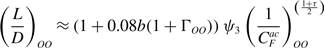 \begin{align}{\left( {\frac{L}{D}} \right)_{OO}} \approx \left( {1 + 0.08b\!\left( {1 + {{\rm{\Gamma }}_{OO}}} \right)} \right){\psi _3}\left( {\frac{1}{{C_F^{ac}}}} \right)_{OO}^{\left( {\frac{{1 + \tau }}{2}} \right)}\end{align}
and
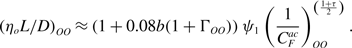 \begin{align}{\left( {{\eta _o}L/D} \right)_{OO}} \approx \left( {1 + 0.08b\!\left( {1 + {{\rm{\Gamma }}_{OO}}} \right)} \right){\psi _1}\left( {\frac{1}{{C_F^{ac}}}} \right)_{OO}^{\left( {\frac{{1 + \tau }}{2}} \right)}.\end{align}
Finally, Equation (46) is used to provide a correction to the Mach number,
 \begin{align}{M_{OO}} \approx {\psi _4}\left( {1 - \frac{{0.10}}{{co{s^2}\left( {{{\rm{\Lambda }}_w}} \right)}}\left( {\frac{{{{\left( {{C_L}} \right)}_{OO}} - {{\left( {{C_L}} \right)}_{DO}}}}{{{{\left( {{M_{CC}}} \right)}_{DO}}}}} \right)} \right).\end{align}
In the Poll and Schumann [2, Reference Poll3] method, $\Psi$
1
,
$\Psi$
1
, $\Psi$
2, and
$\Psi$
2, and $\Psi$
3
are assumed to be constant. However, the solutions developed here, specifically Equations (60), (66) and (67), show that these parameters are Reynolds number dependent. This dependency is both direct and indirect, but, in all cases, it is very weak. Therefore, if these parameters are evaluated at the design condition, they may be taken to be constant without any significant loss of accuracy. The relevant values of
$\Psi$
3
are assumed to be constant. However, the solutions developed here, specifically Equations (60), (66) and (67), show that these parameters are Reynolds number dependent. This dependency is both direct and indirect, but, in all cases, it is very weak. Therefore, if these parameters are evaluated at the design condition, they may be taken to be constant without any significant loss of accuracy. The relevant values of $\Psi$
1
,
$\Psi$
1
, $\Psi$
2 and
$\Psi$
2 and $\Psi$
3
are those listed in Table 3.
$\Psi$
3
are those listed in Table 3.
10. Discussion
As noted in the previous section, Poll and Schumann [Reference Poll3] have already obtained estimates for M
DO
(= $\Psi$
4
) that are adequate for practical application. These can be compared with the estimates obtained using the present approach and the results are given in Fig. 6. The estimates and the data correlate extremely well, but the scatter is ±6%, which is about the expected level due to the uncertainty in the value of intercept in Equation (34). Hence, estimates for M
DO
can only be improved by improving the accuracy of (M
cc
)
DO
and this requires detail that is unlikely to ever appear in the open literature.
$\Psi$
4
) that are adequate for practical application. These can be compared with the estimates obtained using the present approach and the results are given in Fig. 6. The estimates and the data correlate extremely well, but the scatter is ±6%, which is about the expected level due to the uncertainty in the value of intercept in Equation (34). Hence, estimates for M
DO
can only be improved by improving the accuracy of (M
cc
)
DO
and this requires detail that is unlikely to ever appear in the open literature.
Comparison of the estimates of the optimum Mach number with the values given by Poll and Schumann [Reference Poll3]. The dashed lines indicate a deviation of ±6%.
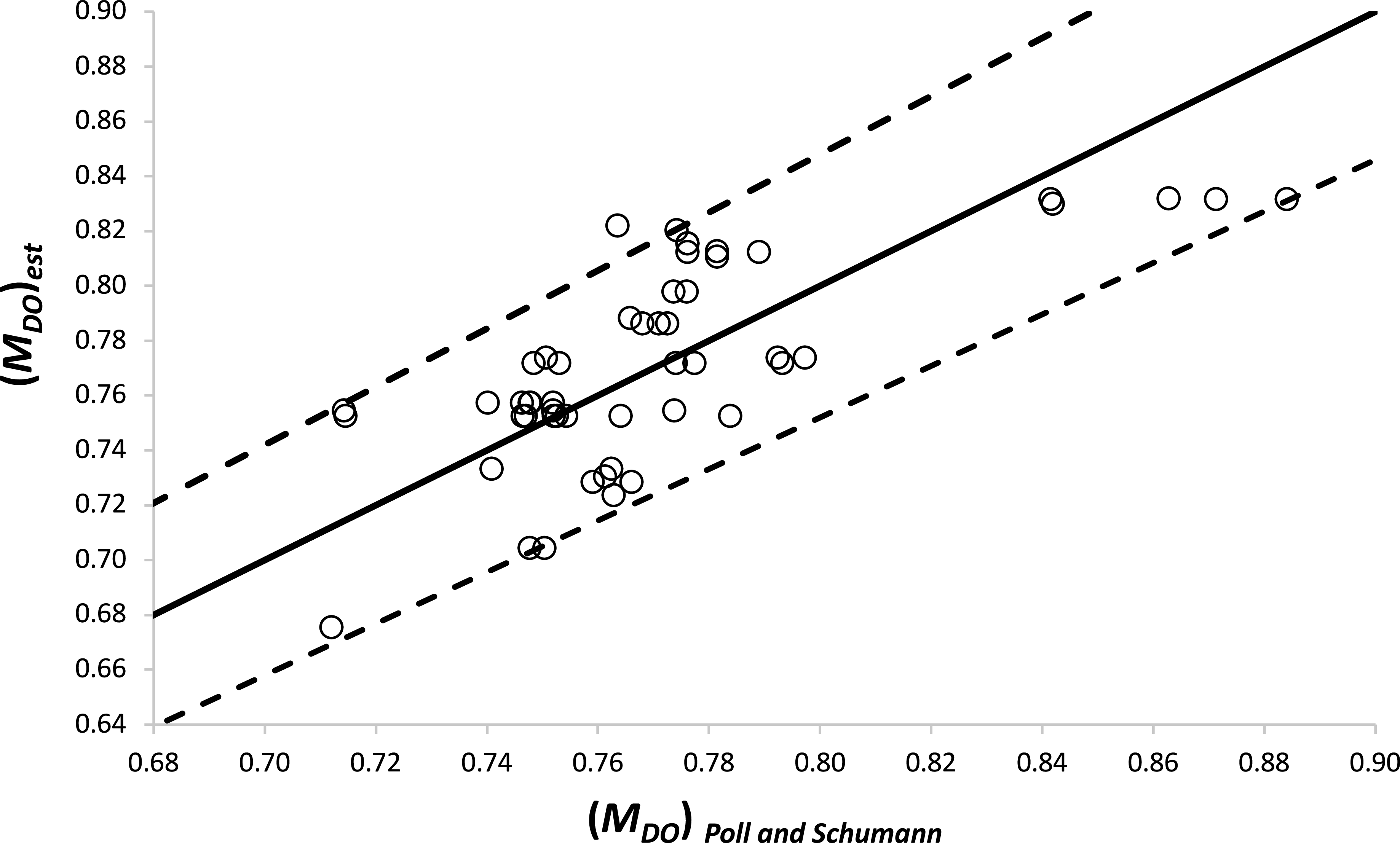
In the current approach, the Poll and Schumann [Reference Poll3] estimates for M DO are combined with the (accurate) estimates of X DO from Equation (45) to obtain a value of (M cc ) DO for each aircraft, i.e.
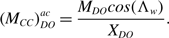 \begin{align}\left( {{M_{CC}}} \right)_{DO}^{ac} = \frac{{{M_{DO}}cos\!\left( {{\Lambda _w}} \right)}}{{{X_{DO}}}}.\end{align}
A “least squares” fit to the resulting values gives
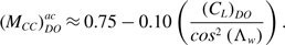 \begin{align}\left( {{M_{CC}}} \right)_{DO}^{ac} \approx 0.75 - 0.10\left( {\frac{{{{\left( {{C_L}} \right)}_{DO}}}}{{co{s^2}\left( {{\Lambda _w}} \right)}}} \right).\end{align}
The close agreement between this result and Equation (34) is a very strong indication that the drag estimates are accurate, but, as already noted, the intrinsic uncertainty is too great for a combination of Equations (46) and either (34) or (88) to yield satisfactory estimates for M DO .
Apart from M
DO
and, consequently, $\delta$
DO
, the uncertainty associated with all the other parameters is very small. The principal finding and the result upon which the estimates are based is that for the Reynolds number for the design (
$\delta$
DO
, the uncertainty associated with all the other parameters is very small. The principal finding and the result upon which the estimates are based is that for the Reynolds number for the design ( $\eta$
o
L/D) – see Equation (63). This depends upon the aircraft’s geometry, the instantaneous aircraft mass, m, and the properties of the atmosphere. Once this quantity is determined, the zero-lift drag coefficient, (Cd
0
)
DO
and the lift-dependent drag factor, K
DO
, follow immediately from Equations (16), (17) and (23). The second key result is the expression for the wave drag coefficient at the design optimum as given in Equation (43), i.e.
$\eta$
o
L/D) – see Equation (63). This depends upon the aircraft’s geometry, the instantaneous aircraft mass, m, and the properties of the atmosphere. Once this quantity is determined, the zero-lift drag coefficient, (Cd
0
)
DO
and the lift-dependent drag factor, K
DO
, follow immediately from Equations (16), (17) and (23). The second key result is the expression for the wave drag coefficient at the design optimum as given in Equation (43), i.e.
 \begin{align}{\left( {C{d_w}} \right)_{DO}} \approx 3.2{\left( {\left( {2{\eta _2} + b} \right)\left( {1 - \left( {\frac{{2 + {\eta _2}}}{{2{\eta _2} + b}}} \right)b\!\left( {1 + {{\rm{\Gamma }}_{DO}}} \right)} \right)} \right)^2}{\left( {\frac{{{{\left( {C{d_0}} \right)}^2}}}{{co{s^3}\!\left( {{{\rm{\Lambda }}_w}} \right)}}} \right)_{DO}}.\end{align}
Taking mid-range values for the various parameters, a typical value for (Cd
w
)
DO
is found to be about 8 drag counts or 2.5% of the total drag. This in consistent with statements in Torenbeek [Reference Jenkinson, Simpkin and Rhodes7] that “compressibility drag in fuel economical flight is typically between 5 and 10 counts’ or about 3% of the total – see Fig. 14.6 of Ref. (Reference Jenkinson, Simpkin and Rhodes7). The wave drag coefficient is found to increases as (Cd
0
)
DO
squared and also as almost $\eta$
2 squared. Consequently, aircraft with a smaller wing area per passenger and using low bypass ratio engines will have the highest values of wave drag at the optimum condition. This situation is typical of the older, short haul, single aisle aircraft. Conversely, long haul, twin aisle aircraft with large wing area per passenger and high bypass ratio engines will have low values. The wave drag also depends upon both the local temperature and the lapse rate.
$\eta$
2 squared. Consequently, aircraft with a smaller wing area per passenger and using low bypass ratio engines will have the highest values of wave drag at the optimum condition. This situation is typical of the older, short haul, single aisle aircraft. Conversely, long haul, twin aisle aircraft with large wing area per passenger and high bypass ratio engines will have low values. The wave drag also depends upon both the local temperature and the lapse rate.
The approximate solution also allows the effects of compressibility and variable Reynolds number on the maximum value of the lift-to-drag ratio and the lift coefficient and Mach number at which it occurs to be identified. As shown, in general, the results may be expressed as
 \begin{align}\;\;{\left( {{L \over D}} \right)_{DO}} \propto {1 \over 2}\left( {{1 \over {KC{d_0}}}} \right)_{DO}^{1/2},\;{\left( {{C_L}} \right)_{DO}} \propto \left( {{{C{d_0}} \over K}} \right)_{DO}^{1/2}\;{\rm{and\;}}{\left( {Cd} \right)_{DO}} \propto 2{\left( {C{d_0}} \right)_{DO}}.\end{align}
When the Reynolds number is constant, i.e. changes in speed and altitude do not change Reynolds number, and there is no wave drag, the constants of proportionality are all unity.
As shown in Equations (50), (51) and (52), when both wave drag and Reynolds number variation are present and the aircraft is flying in the International Standard Atmosphere, the constants of proportionality for flight in the troposphere are found to be about 0.96 for (L/D) DO , 0.92 for (C L ) DO and 0.96 for (Cd) DO , whilst in the stratosphere the constants are 0.96, 0.90 and 0.94, respectively. In all cases, the constants are less than unity. The lowest values occur in the stratosphere and the impact upon (C L ) DO is largest with a reduction of 10%, followed by (Cd) DO with 6% and then (L/D) DO with 4%. These are significant changes, particularly for (C L ) DO .
The reduction in (C L ) DO means that, for an aircraft of given mass flying at the optimum Mach number, the optimum flight level will be reduced relative to the constant Reynolds number, zero wave drag case. In Poll [1] it was found that, in the vicinity of the ISA tropopause,
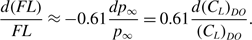 \begin{align}\frac{{d\!\left( {FL} \right)}}{{FL}} \approx - 0.61\frac{{d{p_\infty }}}{{{p_\infty }}} = 0.61\frac{{d{{\left( {{C_L}} \right)}_{DO}}}}{{{{\left( {{C_L}} \right)}_{DO}}}}.\end{align}
Hence, for flight in the troposphere, the reduction in cruise altitude due to compressibility and Reynolds number variation is about 1,750 feet. When the aircraft leaves the troposphere and enters the stratosphere, (C L ) DO drops by an additional 2%, giving a further reduction of about 450 feet.
The approximate solution also allows the separation of the compressibility and Reynolds number effects. Reynolds number variation is removed by setting the constant b equal to zero. In this case, the constants of proportionality are the same for flight in both troposphere and stratosphere, becoming 0.95 for (L/D) DO , 0.985 for (C L ) DO and 1.035 for (Cd) DO . Therefore, through compressibility effects alone, (L/D) DO is reduced by about 5% and (C L ) DO is reduced by just 1.5%, whilst (Cd) DO is increased by 3.5%. Consequently, compressibility effects alone would account for a reduction in cruise altitude of only about FL 3.5, or 350 feet. The conclusion is that (L/D) DO is controlled primarily by compressibility effects, as shown in Equation (42), whilst the values of C L and Cd at the design condition are largely determined by the Reynolds number variation, i.e. by the value of the coefficient b.
Generally, the surface of an aircraft is never perfectly smooth and, in the early days of civil jet transport, the surface quality could deteriorate quite quickly in routine operations. In extreme cases, the surface could become “aerodynamically rough”, with the drag coefficient being a constant determined by the scale of the roughness, see, e.g. Obert [Reference Obert15] (Chapter 40). In this case, b is zero. As indicated in Equations (50) to (52), in this situation, the changes to (L/D) DO , (C L ) DO and (Cd) DO are both relatively small and have no dependence upon the nature of the atmosphere. Since most of the standard texts on aircraft performance were written many years ago, this may explain why the effects of wave drag receive so little attention. More recently, with the progressive improvement in manufacturing processes and the development of better paints, modern surfaces tend to be “aerodynamically smooth”, but with the boundary layers on the wing and fuselage usually still in the fully turbulent state, i.e. b is about 0.14.
Looking to the future, one of the most effective ways to reduce fuel consumption is to produce aircraft that can support extensive areas of laminar flow on the wing, the empennage and, possibly, the fuselage. This is because advanced materials and manufacturing techniques can now deliver extremely smooth surfaces with very few, or no, steps, or gaps, and very small waviness. These surfaces can also be perforated to allow the use of weak, surface suction to increase the stability of the laminar boundary layer and delay transition to turbulence to higher Reynolds numbers. The first generation of these aircraft are likely to see a 10% to 15% reduction in the Cd 0 resulting from limited regions of laminar flow on the wings and empennage and, from Equation (52), this will give a 5 to 7.5% increase in (L/D) DO , with a corresponding reduction in the required fuel flow rate. However, as can be seen from Equation (50), this change in Cd 0 also reduces (C L ) DO by 5% to 7.5%, corresponding to a reduction in the optimum cruise altitude of between 1000 and 1500 feet. Furthermore, the existence of any regions of laminar flow will increase the value of the coefficient, b, in the skin friction law (Equation (17)). This is because, in pure laminar flow, b is equal to 0.5 – see Shevell [Reference Shevell8]. Therefore, as the area covered by laminar flow increases and that covered by turbulent flow decreases, b must increase progressively from the current value of 0.14 to 0.5 and the constant of proportionality in Equation (50) will drop from about 0.9 to about 0.7. The combined effects of a reduction in Cd 0 and an increase in b will produce a significant lowering of the design optimum and, hence, the operational optimum cruise altitudes for these “advanced” aircraft. In addition, for a given aircraft, the improvement in (L/D) DO reduces the fuel required and, hence, the operational mass of the aircraft. This increases the optimum cruise altitude. However, it is demonstrated in Appendix E that, all other things being equal, the reduction in (C L ) DO is always the dominant effect. Consequently, the application of drag reducing technology to lower Cd 0 will always reduce the optimum cruise altitude.
Up to the present time, the evolutionary trend has been one of incremental improvements in engine overall efficiency and increases in airframe aerodynamic efficiency – through higher wing aspect ratios and small reductions in Cd 0 – see Poll [Reference Poll18]. The primary impact has been reduced trip fuel and the net effect is that optimum cruise altitudes have been rising slowly over time. The potential reversal of this trend by the introduction of novel technologies may have implications for the aircraft’s environmental impact and deserves further consideration.
11.0 Conclusions
A turbofan powered, civil transport aircraft, with a specified weight and operating in a specified atmosphere, has its lowest possible fuel burn at a particular value of Mach number and flight level. These optimum operating conditions are governed by two partial differential equations, involving characteristics of both airframe and engine. However, for fixed Mach number cruise, the airframe lift-drag ratio and the engine overall efficiency both exhibit local maxima with respect to drag and, hence, thrust. Consequently, an absolute optimum is obtained when both parameters peak at the same Mach number and flight level. It is shown that this “perfect” matching of components can only be achieved at one particular set of conditions, termed the “design optimum” and the corresponding Mach number and flight level are fundamental characteristics of the aircraft-engine combination. Consequently, the governing differential equations for the general optimum have been used to describe the design optimum conditions in a completely general atmosphere. An approximate solution has been developed using established aerodynamic theory and a simple, aircraft bespoke, wave drag model that also allows the wave drag to be estimated at Mach numbers and flight levels far removed from the design optimum values. The solution has been used to estimate the influence of compressibility and Reynolds number both collectively and separately. Relative to the “classic text book” situation with constant Reynolds number and zero wave drag, it is found that L/D at the design optimum is hardly affected by changes in Reynolds number, but it is reduced by about 5% due to compressibility effects. Conversely, the corresponding values of lift and drag coefficients are reduced by about 10% and 6% respectively, primarily, due to variations in Reynolds number. Therefore, the effect of Reynolds number variation due to changes in flight level is significant.
In general, the flight conditions for the operating optimum will not be the same as the design optimum due to differences in aircraft weight and atmospheric conditions. However, since these variations are generally small, it has been possible to adapt a previously published method to estimate the optimum operating conditions for any aircraft weight and any atmospheric conditions, using the design optimum condition as the datum case.
Finally, some small changes have been made to previously published coefficients to improve the accuracy of the estimates. The revised parameter values are given in tabular form.
Looking ahead, comparisons are being conducted between the PS model and a number of sets of data from open sources, plus a few observations from other models. Preliminary results indicate that differences between the PS model and specific data sets can be largely removed by minor adjustments to some of the input parameters, but no changes to the model structure are required.
Appendix A. Estimation of the lift and drag coefficients at the design optimum condition
Differentiation of the drag polar shown in Equation (15) gives
 \begin{align}\frac{{{M_\infty }}}{{Cd}}\frac{{\partial Cd}}{{\partial {M_\infty }}} = \frac{{C{d_0}}}{{Cd}}\left( {\left( {\frac{{{M_\infty }}}{{C{d_0}}}\frac{{\partial C{d_0}}}{{\partial {M_\infty }}}} \right) - \left( {4 - \left( {\frac{{{M_\infty }}}{K}\frac{{\partial K}}{{\partial {M_\infty }}}} \right)} \right)\left( {\frac{{KC_L^2}}{{C{d_0}}}} \right) + \left( {\frac{{{M_\infty }}}{{C{d_0}}}\frac{{\partial C{d_w}}}{{\partial {M_\infty }}}} \right)} \right)\end{align}
and
 \begin{align}\frac{{{C_L}}}{{Cd}}\frac{{\partial Cd}}{{\partial {C_L}}} = \frac{{C{d_0}}}{{Cd}}\left( {\left( {\frac{{{C_L}}}{{C{d_o}}}\frac{{\partial C{d_0}}}{{\partial {C_L}}}} \right) + \left( {2 + \left( {\frac{{{C_L}}}{K}\frac{{\partial K}}{{\partial {C_L}}}} \right)} \right)\left( {\frac{{KC_L^2}}{{C{d_0}}}} \right) + \left( {\frac{{{C_L}}}{{C{d_0}}}\frac{{\partial C{d_w}}}{{\partial {C_L}}}} \right)} \right).\end{align}
Using Equations (16) and (17),
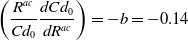 \begin{align}\left( {\frac{{{R^{ac}}}}{{C{d_0}}}\frac{{dC{d_0}}}{{d{R^{ac}}}}} \right) = - b = - 0.14\end{align}
and, from Equation (4),
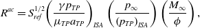 \begin{align}{R^{ac}} = S_{ref}^{1/2}{\left( {\frac{{\gamma {p_{TP}}}}{{{\mu _{TP}}{a_{TP}}}}} \right)_{ISA}}\left( {\frac{{{p_\infty }}}{{{{\left( {{p_{TP}}} \right)}_{ISA}}}}} \right)\left( {\frac{{{M_\infty }}}{\phi }} \right),{\rm{\;}}\end{align}
where the subscript TP refers to conditions at the tropopause. Furthermore, as shown by Poll and Schumann [2], in a general atmosphere,
 \begin{align}\phi = {{{\mu _\infty }{a_\infty }} \over {{{\left( {{\mu _{TP}}{a_{TP}}} \right)}_{ISA}}}} \approx {\left( {{{{T_\infty }} \over {{{\left( {{T_{TP}}} \right)}_{ISA}}}}} \right)^{1.34}} \approx \left( {1 + 1.34{{{\rm{\Delta }}T} \over {{{\left( {{T_{TP}}} \right)}_{ISA}}}}} \right)\left( {{{{T_\infty }} \over {{T_{TP}}}}} \right)_{ISA}^{1.34} \approx \left( {1 + 1.34\overline {\Delta T} } \right){\left( {{{{{\left( {{p_{TP}}} \right)}_{ISA}}} \over {{p_\infty }}}} \right)^{1.34\omega }}.\end{align}
where $\Delta T$
is the difference between the actual temperature and the temperature in the International Standard Atmosphere [Reference Poll and Schumann4] at the same flight level and
$\Delta T$
is the difference between the actual temperature and the temperature in the International Standard Atmosphere [Reference Poll and Schumann4] at the same flight level and $\omega$
is a constant. Hence,
$\omega$
is a constant. Hence,
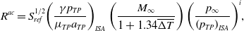 \begin{align}{R^{ac}} = S_{ref}^{1/2}{\left( {{{\gamma {p_{TP}}} \over {{\mu _{TP}}{a_{TP}}}}} \right)_{ISA}}\left( {{{{M_\infty }} \over {1 + 1.34\overline {\Delta T} }}} \right){\left( {{{{p_\infty }} \over {{{\left( {{p_{TP}}} \right)}_{ISA}}}}} \right)^i},\end{align}
with
 \begin{align}\iota = 1 + 1.34\omega .\end{align}
If p
∞
is greater than, or equal to, (p
TP
)
ISA
, i.e. p
∞
≥ 226.32 hPa, $\omega$
is −0.19026 and
$\omega$
is −0.19026 and $\iota$
is 0.74505 and, if p
∞
is less than (p
TP
)
ISA
,
$\iota$
is 0.74505 and, if p
∞
is less than (p
TP
)
ISA
, $\omega$
is zero and
$\omega$
is zero and $\iota$
is equal to one. In addition, when the Mach number is constant,
$\iota$
is equal to one. In addition, when the Mach number is constant,
 \begin{align}\left( {\frac{{{p_\infty }}}{{{R^{ac}}}}\frac{{\partial {R^{ac}}}}{{\partial {p_\infty }}}} \right) = 1 - \left( {\frac{{{p_\infty }}}{\phi }\frac{{\partial \phi }}{{\partial {p_\infty }}}} \right) = 1 + {\rm{\Gamma }}.\end{align}
In the special case of the International Standard Atmosphere,
 \begin{align}{\rm{\Gamma }} \approx \iota - 1 = 1.34\omega ,\end{align}
whilst, in a completely general atmosphere, as demonstrated in Poll and Schumann [2],
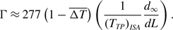 \begin{align}{\rm{\Gamma }} \approx 277\left( {1 - \overline {\Delta T} } \right)\left( {{1 \over {{{\left( {{T_{TP}}} \right)}_{ISA}}}}{{{d_\infty }} \over {dL}}} \right).\end{align}
Hence, from Equations (7), (A-3), (A-4) and (A-8),
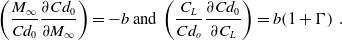 \begin{align}\left( {\frac{{{M_\infty }}}{{C{d_0}}}\frac{{\partial C{d_0}}}{{\partial {M_\infty }}}} \right) = - b{\rm{\;and\;}}\left( {\frac{{{C_L}}}{{C{d_o}}}\frac{{\partial C{d_0}}}{{\partial {C_L}}}} \right) = b\!\left( {1 + {\rm{\Gamma }}} \right)\;.\;\end{align}
Also, from Equations (22) and (23),
 \begin{align}\left( {\frac{{{C_L}}}{K}\frac{{\partial K}}{{\partial {C_L}}}} \right) = \frac{{{k_1}}}{K}\left( {\frac{{{C_L}}}{{C{d_o}}}\frac{{\partial C{d_0}}}{{\partial {C_L}}}} \right)\;{\rm{and}}\;\left( {\frac{{{M_\infty }}}{K}\frac{{\partial K}}{{\partial {M_\infty }}}} \right) = \frac{{{k_1}}}{K}\left( {\frac{{{M_\infty }}}{{C{d_0}}}\frac{{\partial C{d_0}}}{{\partial {M_\infty }}}} \right){\rm{\;}}.\end{align}
Equations (A-1) and (A-2) then become
 \begin{align}\frac{{{M_\infty }}}{{Cd}}\frac{{\partial Cd}}{{\partial {M_\infty }}} = \frac{{C{d_0}}}{{Cd}}\left( {\left( {\frac{{{M_\infty }}}{{C{d_0}}}\frac{{\partial C{d_w}}}{{\partial {M_\infty }}}} \right) - b - \left( {4 + \left( {\frac{{{k_1}}}{K}} \right)b} \right)\left( {\frac{{KC_L^2}}{{C{d_0}}}} \right)} \right)\end{align}
and
 \begin{align}\frac{{{C_L}}}{{Cd}}\frac{{\partial Cd}}{{\partial {C_L}}} = \frac{{C{d_0}}}{{Cd}}\left( {\left( {\frac{{{C_L}}}{{C{d_0}}}\frac{{\partial C{d_w}}}{{\partial {C_L}}}} \right) + b\!\left( {1 + {\rm{\Gamma }}} \right) + \left( {2 + \left( {\frac{{{k_1}}}{K}} \right)b\!\left( {1 + {\rm{\Gamma }}} \right)} \right)\left( {\frac{{KC_L^2}}{{C{d_0}}}} \right)} \right).\end{align}
Therefore, at the design optimum, Equations (13), (14), (15), (A-13) and (A-14) combine to give
 \begin{align}{\left( {\frac{{{M_\infty }}}{{C{d_0}}}\frac{{\partial C{d_w}}}{{\partial {M_\infty }}}} \right)_{DO}} = \left( {2 + {\eta _2} + \left( {\frac{{{k_1}}}{K}} \right)b} \right){\left( {\frac{{KC_L^2}}{{C{d_0}}}} \right)_{DO}} - \left( {2 - {\eta _2}} \right){\left( {\frac{{C{d_w}}}{{C{d_0}}}} \right)_{DO}} - \left( {2{ -{\eta _2}} - b} \right)\end{align}
and
 \begin{align}{\left( {\frac{{{C_L}}}{{C{d_0}}}\frac{{\partial C{d_w}}}{{\partial {C_L}}}} \right)_{DO}} = \left( {1 - b\!\left( {1 + {{\rm{\Gamma }}_{DO}}} \right)} \right) + {\left( {\frac{{C{d_w}}}{{C{d_0}}}} \right)_{DO}} - \left( {1 + \left( {\frac{{{k_1}}}{K}} \right)b\!\left( {1 + {{\rm{\Gamma }}_{DO}}} \right)} \right){\left( {\frac{{KC_L^2}}{{C{d_0}}}} \right)_{DO}}.\end{align}
In addition, rearranging Equation (A-16) and neglecting quantities that are small compared to unity gives
 \begin{align}{\left( {{C_L}} \right)_{DO}} \approx \left( {1 - {1 \over 2}\left( {b\!\left( {1 + \left( {{{{k_1}} \over K}} \right)} \right)\left( {1 + {{\rm{\Gamma }}_{DO}}} \right) + {{\left( {{{C{d_w}} \over {C{d_0}}}} \right)}_{DO}}\left( {{{\left( {{{{C_L}} \over {C{d_w}}}{{\partial C{d_w}} \over {\partial {C_L}}}} \right)}_{DO}} - 1} \right)} \right)} \right)\left( {{{C{d_0}} \over K}} \right)_{DO}^{1/2}\end{align}
and, using Equation (15),
 \begin{align}{\left( {Cd} \right)_{DO}} \approx 2\left( {1 - \frac{1}{2}\left( {b\!\left( {1 + \left( {\frac{{{k_1}}}{K}} \right)} \right)\left( {1 + {{\rm{\Gamma }}_{DO}}} \right) + {{\left( {\frac{{C{d_w}}}{{C{d_0}}}} \right)}_{DO}}\left( {{{\left( {\frac{{{C_L}}}{{C{d_w}}}\frac{{\partial C{d_w}}}{{\partial {C_L}}}} \right)}_{DO}} - 2} \right)} \right)} \right){\left( {C{d_0}} \right)_{DO}}.\end{align}
Hence,
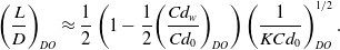 \begin{align}{\left( {{L \over D}} \right)_{DO}} \approx {1 \over 2}\left( {1 - {1 \over 2}{{\left( {{{C{d_w}} \over {C{d_0}}}} \right)}_{DO}}} \right)\left( {{1 \over {KC{d_0}}}} \right)_{DO}^{1/2}.\end{align}
Appendix B. An approximate solution for the wave drag at the design optimum condition
For simplicity, let
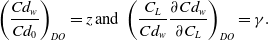 \begin{align}{\left( {\frac{{C{d_w}}}{{C{d_0}}}} \right)_{DO}} = z\;{\rm{and}}\;\;{\left( {\frac{{{C_L}}}{{C{d_w}}}\frac{{\partial C{d_w}}}{{\partial {C_L}}}} \right)_{DO}} = \gamma .\end{align}
Noting that, since (k 1 /K) is of order 0.1 and b is equal to 0.14, their product is of order 0.01, which is small compared to unity, Equations (A-15) and (A-16) can be written as
 \begin{align}{\left( {\frac{{{M_\infty }}}{{C{d_0}}}\frac{{\partial C{d_w}}}{{\partial {M_\infty }}}} \right)_{DO}} \approx \left( {2 + {\eta _2}} \right){\left( {\frac{{KC_L^2}}{{C{d_0}}}} \right)_{DO}} - \left( {2 - {\eta _2}} \right)z - \left( {2 - {\eta _2} - b} \right)\end{align}
and
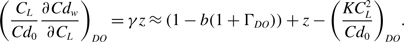 \begin{align}{\left( {\frac{{{C_L}}}{{C{d_0}}}\frac{{\partial C{d_w}}}{{\partial {C_L}}}} \right)_{DO}} = \gamma z \approx \left( {1 - b\!\left( {1 + {{\rm{\Gamma }}_{DO}}} \right)} \right) + z - {\left( {\frac{{KC_L^2}}{{C{d_0}}}} \right)_{DO}}.\end{align}
Hence,
 \begin{align}{\left( {\frac{{{M_\infty }}}{{C{d_0}}}\frac{{\partial C{d_w}}}{{\partial {M_\infty }}}} \right)_{DO}} \approx \left( {2{\eta _2} - b\!\left( {\left( {1 + {{\rm{\Gamma }}_{DO}}} \right)\left( {2 + {\eta _2}} \right) - 1} \right)} \right) - \left( {\gamma \!\left( {2 + {\eta _2}} \right) - 2{\eta _2}} \right)z.\end{align}
Using Equation (39),
 \begin{align}\left( {2{\eta _2} - b\!\left( {\left( {1 + {{\rm{\Gamma }}_{DO}}} \right)\left( {2 + {\eta _2}} \right) - 1} \right)} \right) - \left( {\gamma \!\left( {2 + {\eta _2}} \right) - 2{\eta _2}} \right)z = 2z\left( {1 - {\delta _{DO}}} \right){\left( {\frac{X}{{X - {j_2}}}} \right)_{DO}}\end{align}
and, using equation (40),
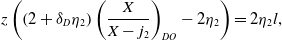 \begin{align}z\left( {\left( {2 + {\delta _D}{\eta _2}} \right){{\left( {\frac{X}{{X - {j_2}}}} \right)}_{DO}} - 2{\eta _2}} \right) = 2{\eta _2}l,\end{align}
where
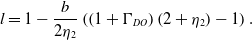 \begin{align}l = 1 - \frac{b}{{2{\eta _2}}}\left( {\left( {1 + {{\rm{\Gamma }}_{DO}}} \right)\left( {2 + {\eta _2}} \right) - 1} \right).\end{align}
Rearranging Equation (B-6), using Equation (38) and setting
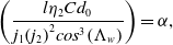 \begin{align}\left( {\frac{{l{\eta _2}C{d_0}}}{{{j_1}{{\left( {{j_2}} \right)}^2}co{s^3}\!\left( {{{\rm{\Lambda }}_w}} \right)}}} \right) = \alpha ,\end{align}
gives
 \begin{align}X_{DO}^2\left( {2 - \left( {2 - {\delta _{DO}}} \right){\eta _2}} \right) - {X_{DO}}\!\left( {2 - \left( {4 - {\delta _o}} \right){\eta _2}} \right){j_2} - 2{b^2}\left( {{\eta _2} + \alpha } \right) = 0.\end{align}
The exact solution is given by the positive value of
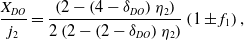 \begin{align}\frac{{{X_{DO}}}}{{{j_2}}} = \frac{{\left( {2 - \left( {4 - {\delta _{DO}}} \right){\eta _2}} \right)}}{{2\left( {2 - \left( {2 - {\delta _{DO}}} \right){\eta _2}} \right)}}\left( {1 \pm {f_1}} \right),\end{align}
where
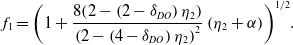 \begin{align}{f_1} = {\left( {1 + \frac{{8\!\left( {2 - \left( {2 - {\delta _{DO}}} \right){\eta _2}} \right)}}{{{{\left( {2 - \left( {4 - {\delta _{DO}}} \right){\eta _2}} \right)}^2}}}\left( {{\eta _2} + \alpha } \right)} \right)^{1/2}}.\end{align}
Hence,
 \begin{align}z = {j_1}{\left( {{X_{DO}} - {j_2}} \right)^2}\left( {\frac{{co{s^3}\!\left( {{{\rm{\Lambda }}_w}} \right)}}{{{{\left( {C{d_0}} \right)}_{DO}}}}} \right) = \left( {\frac{{co{s^3}\!\left( {{{\rm{\Lambda }}_w}} \right){j_1}{{\left( {{j_2}} \right)}^2}}}{{4{{\left( {C{d_0}} \right)}_{DO}}{{\left( {2 - \left( {2 - {\delta _{DO}}} \right){\eta _2}} \right)}^2}}}} \right){f_2},\end{align}
where
 \begin{align}{f_2} = {\left( {\left( {2 - \left( {4 - {\delta _{DO}}} \right){\eta _2}} \right){f_1} - (2 + {\delta _{DO}}{\eta _2}} \right)^2}.\end{align}
Based upon the earlier work of Poll and Schumann [2, Reference Poll3], the expected parameter ranges for the current global aircraft fleet are
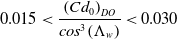 \begin{align}0.015 \lt \frac{{{{\left( {C{d_0}} \right)}_{DO}}}}{{co{s^3}\!\left( {{{\rm{\Lambda }}_w}} \right)}} \lt 0.030\end{align}
and
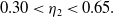 \begin{align}0.30 \lt {\eta _2} \lt 0.65.\end{align}
In addition,
 \begin{align}0.6 \lt \frac{{{{\left( {{C_L}} \right)}_{DO}}}}{{co{s^2}\left( {{{\rm{\Lambda }}_w}} \right)}} \lt 0.75\;\end{align}
and, hence, from Equations (34) and (41),
 \begin{align}0.15 \lt {\delta _{DO}} \lt 0.25.\end{align}
The variation of the function f
2
with $\alpha$
when
$\alpha$
when $\eta$
2 is 0.50 and
$\eta$
2 is 0.50 and $\delta$
DO
is 0.2. The solid line is the exact result and the dashed line is the parabolic approximation.
$\delta$
DO
is 0.2. The solid line is the exact result and the dashed line is the parabolic approximation.
Therefore, in practice, the range of values for f
2
and $\alpha$
are bounded and, as shown in Fig. B-1, when f
2
is plotted as a function of for constant values of
$\alpha$
are bounded and, as shown in Fig. B-1, when f
2
is plotted as a function of for constant values of $\eta$
2 and
$\eta$
2 and $\delta$
DO, the variation in the range of interest is almost parabolic, i.e.
$\delta$
DO, the variation in the range of interest is almost parabolic, i.e.
 \begin{align}{f_2} \approx {\left( {F\alpha } \right)^2}.\end{align}
where F is a constant whose value depends only upon $\eta_{2}$
and
$\eta_{2}$
and $\delta_{DO}$
. The values of F were chosen to give the best fit over the mid-range with equal deviations at the extremes, with the maximum deviation from the exact solution being about
$\delta_{DO}$
. The values of F were chosen to give the best fit over the mid-range with equal deviations at the extremes, with the maximum deviation from the exact solution being about $\pm$
10%. Using equation (B-7), it follows that follows that
$\pm$
10%. Using equation (B-7), it follows that follows that
 \begin{align}z &\approx {\left( {\frac{{{\eta _2}lF}}{{2\left( {2 - \left( {2 - {\delta _{DO}}} \right){\eta _2}} \right)}}} \right)^2}\left( {\frac{{{{\left( {C{d_0}} \right)}_o}}}{{{j_1}{{\left( {{j_2}} \right)}^2}co{s^3}\!\left( {{{\rm{\Lambda }}_w}} \right)}}} \right) \nonumber\\[5pt] &\approx {f_3}{\left( {\frac{{2{\eta _2} + b}}{{2{\eta _2}}}} \right)^2}{\left( {1 - \left( {\frac{{2 + {\eta _2}}}{{2{\eta _2} + b}}} \right)b\!\left( {1 + {{\rm{\Gamma }}_{DO}}} \right)} \right)^2}\left( {\frac{{{{\left( {C{d_0}} \right)}_o}}}{{{j_1}{{\left( {{j_2}} \right)}^2}co{s^3}\!\left( {{{\rm{\Lambda }}_w}} \right)}}} \right),\end{align}
where
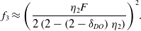 \begin{align}{f_3} \approx {\left( {\frac{{{\eta _2}F}}{{2\left( {2 - \left( {2 - {\delta _{DO}}} \right){\eta _2}} \right)}}} \right)^2}.\end{align}
The variation over the full parameter range is shown in Fig. B-2, where the effect of $\delta$
DO
is clearly very small and may be neglected.
$\delta$
DO
is clearly very small and may be neglected.
The variation of the function f
3
with $\eta$
2 and
$\eta$
2 and $\delta$
DO
. The solid line is the result for
$\delta$
DO
. The solid line is the result for $\delta$
DO
equal to 0.2, the open circles are for
$\delta$
DO
equal to 0.2, the open circles are for $\delta$
DO
of 0.15 and the open diamonds are for
$\delta$
DO
of 0.15 and the open diamonds are for $\delta$
DO
of 0.15.
$\delta$
DO
of 0.15.
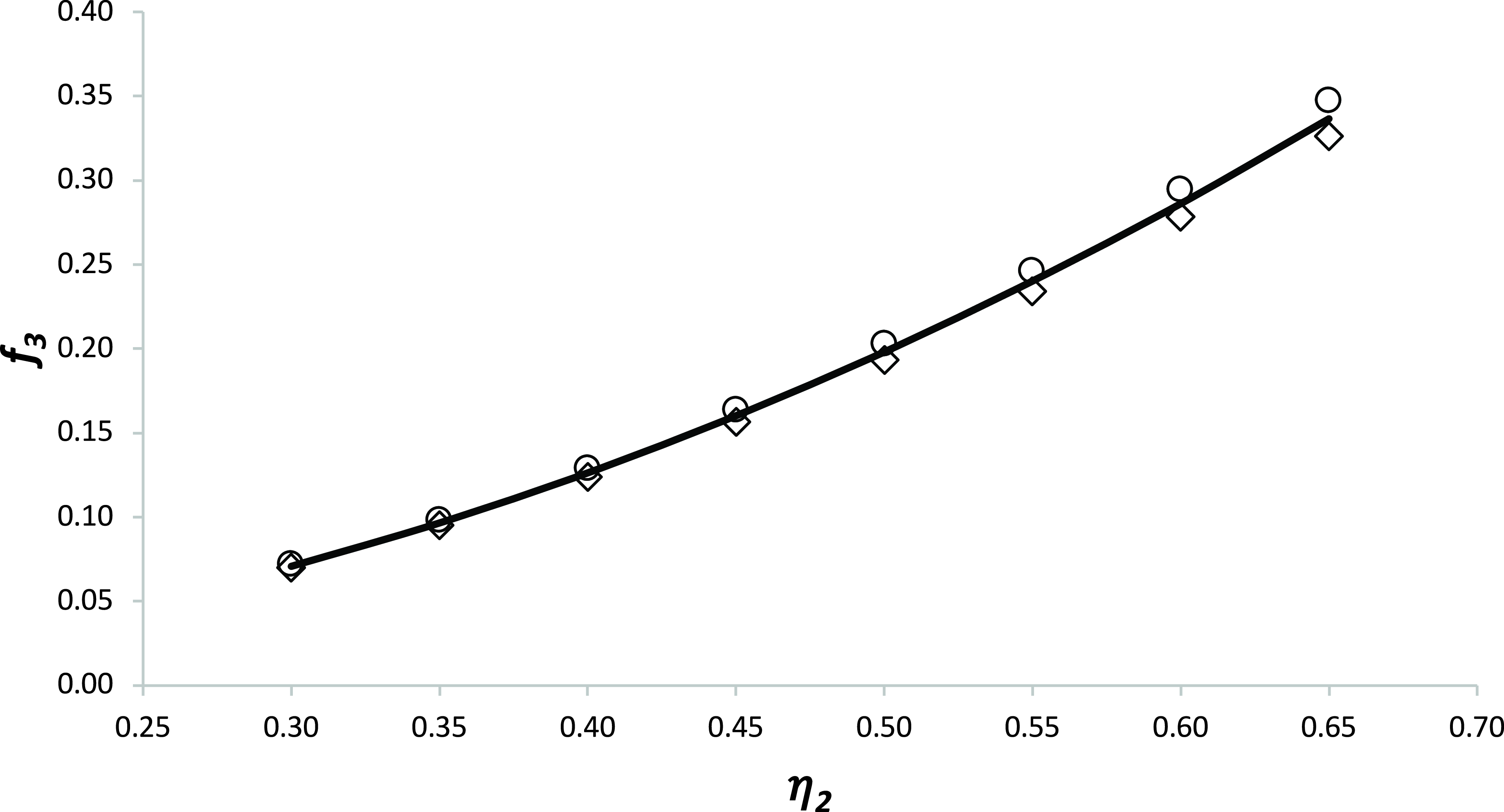
A “least-squares” fit to get the best value of f 3 over the full variable range yields
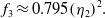 \begin{align}{f_3} \approx 0.795{\left( {{\eta _2}} \right)^2}.\end{align}
The error introduced by neglecting $\delta$
DO
is less than ± 3%. Since this result is insensitive to
$\delta$
DO
is less than ± 3%. Since this result is insensitive to $\delta$
DO
it is also insensitive to uncertainties in the values of the coefficients in Equation (50).
$\delta$
DO
it is also insensitive to uncertainties in the values of the coefficients in Equation (50).
Finally,
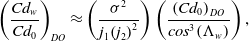 \begin{align}{\left( {\frac{{C{d_w}}}{{C{d_0}}}} \right)_{DO}} \approx \left( {\frac{{{\sigma ^2}}}{{{j_1}{{\left( {{j_2}} \right)}^2}}}} \right)\left( {\frac{{{{\left( {C{d_0}} \right)}_{DO}}}}{{co{s^3}\!\left( {{{\rm{\Lambda }}_w}} \right)}}} \right),\end{align}
where
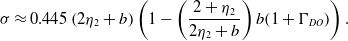 \begin{align}\sigma \approx 0.445\left( {2{\eta _2} + b} \right)\left( {1 - \left( {\frac{{2 + {\eta _2}}}{{2{\eta _2} + b}}} \right)b\!\left( {1 + {{\rm{\Gamma }}_{DO}}} \right)} \right).\end{align}
Appendix C. The approximate variation of the low-speed Oswald efficiency factor with the drag coefficient
The low-speed value of the Oswald efficiency factor is given by Equations (20), (21) and (22). However, to simplify the mathematical manipulations, an approximate power law form is required, i.e.
 \begin{align}{e_{LS}} \approx \frac{E}{{{{\left( {C_F^{ac}} \right)}^\tau }}}\;{\rm{where}}\;\tau = - \left( {\frac{{C_F^{ac}}}{{{e_{LS}}}}} \right)\frac{{d{e_{LS}}}}{{dC_F^{ac}}}.\end{align}
From Equation (20),
 \begin{align}\frac{{d{e_{LS}}}}{{d{k_1}}} = - \left( {\pi .AR} \right)e_{LS}^2\end{align}
and, from Equation (22),
 \begin{align}\frac{{d{k_1}}}{{dC_F^{ac}}} = \frac{{{k_1}}}{{C_F^{ac}}}.\end{align}
Hence,
 \begin{align}\tau = - \left( {\frac{{C_F^{ac}}}{{{e_{LS}}}}} \right)\left( { - \left( {\pi .AR} \right)e_{LS}^2} \right)\frac{{{k_1}}}{{C_F^{ac}}} = \pi .AR.{k_1}{e_{LS}},\end{align}
and
 \begin{align}E = {e_{LS}}{\left( {C_F^{ac}} \right)^\tau }.\end{align}
Appendix D. Relations linking static pressure, indicated altitude and flight level
As described in Poll [1] and Poll and Schumann [2], “altitude” is determined by comparing ambient static pressure, p ∞ with a reference pressure, p ref , specified by Air Traffic Management (ATM). The altimeter then provides an indicated altitude (IA) by using the variation of height versus p ∞ /p ref in the International Standard Atmosphere [6]. For take-off and landing, p ref is the local airport pressure (the QFE) and so IA is measured relative to the runway. At an ATM specified height above the airport, p ref is set to the actual pressure at sea level (the QNH or “regional” pressure) and, consequently, the IA is measured relative to sea level. Finally, as the aircraft passes through the ATM determined “transition” altitude, p ref is set to the ISA sea level pressure (1.01325 bars) and the IA is the height above sea level that the aircraft would have in the ISA. Since the vertical variation of ambient pressure and temperature on any particular day is unlikely to be the same as in the ISA, the indicated altitude will probably not be the true geometric value. To avoid any ambiguity, above the transition altitude, the term flight level (FL) is used. Therefore, an aircraft flying at a fixed flight level is following an isobar. Flight level is defined as the indicated altitude divided by 100. Hence, if the ambient pressure is given in bars, when p ∞ is greater than 0.2263204 bars, the flight level is
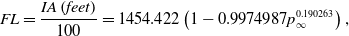 \begin{align}FL = \frac{{IA\left( {feet} \right)}}{{100}} = 1454.422\left( {1 - 0.9974987p_\infty ^{0.190263}} \right),\end{align}
otherwise
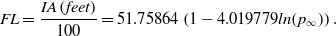 \begin{align}FL = \frac{{IA\left( {feet} \right)}}{{100}} = 51.75864\left( {1 - 4.019779ln\!\left( {{p_\infty }} \right)} \right).\end{align}
Appendix E. An estimate of the effect of reducing Cd 0 on the optimum cruise flight level
Differentiating Equations (50) and (51) gives
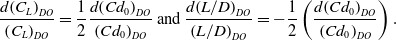 \begin{align}\frac{{d{{\left( {{C_L}} \right)}_{DO}}}}{{{{\left( {{C_L}} \right)}_{DO}}}} = \frac{1}{2}\frac{{d{{\left( {C{d_0}} \right)}_{DO}}}}{{{{\left( {C{d_0}} \right)}_{DO}}}}\;{\rm{and}}\;\frac{{d{{\left( {L/D} \right)}_{DO}}}}{{{{\left( {L/D} \right)}_{DO}}}} = - \frac{1}{2}\left( {\frac{{d{{\left( {C{d_0}} \right)}_{DO}}}}{{{{\left( {C{d_0}} \right)}_{DO}}}}} \right).\end{align}
From Equation (3), the total fuel required for the flight, usually called the trip fuel, (m f ) trip , is almost inversely proportional to L/D and so
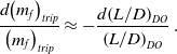 \begin{align}\frac{{d{{\left( {{m_f}} \right)}_{trip}}}}{{{{\left( {{m_f}} \right)}_{trip}}}} \approx - \frac{{d{{\left( {L/D} \right)}_{DO}}}}{{{{\left( {L/D} \right)}_{DO}}}}\;.\end{align}
Hence, since the take-off aircraft mass, MTO, is the sum of the trip fuel mass and a constant mass comprising the structure weight, the pay load and the reserve fuel,
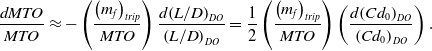 \begin{align}\frac{{dMTO}}{{MTO}} \approx - \left( {\frac{{{{\left( {{m_f}} \right)}_{trip}}}}{{MTO}}} \right)\frac{{d{{\left( {L/D} \right)}_{DO}}}}{{{{\left( {L/D} \right)}_{DO}}}} = \frac{1}{2}\left( {\frac{{{{\left( {{m_f}} \right)}_{trip}}}}{{MTO}}} \right)\left( {\frac{{d{{\left( {C{d_0}} \right)}_{DO}}}}{{{{\left( {C{d_0}} \right)}_{DO}}}}} \right).\end{align}
Near the tropopause, the variation of flight level with ambient pressure is given approximately by Equation (91). Therefore, if (C L ) DO changes due to a change in Cd 0 ,
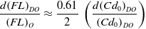 \begin{align}\frac{{d{{\left( {FL} \right)}_{DO}}}}{{{{\left( {FL} \right)}_O}}} \approx \frac{{0.61}}{2}\;\left( {\frac{{d{{\left( {C{d_0}} \right)}_{DO}}}}{{{{\left( {C{d_0}} \right)}_{DO}}}}} \right)\end{align}
and, if (m f ) trip changes due to a change in Cd 0 ,
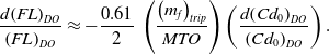 \begin{align}\frac{{d{{\left( {FL} \right)}_{DO}}}}{{{{\left( {FL} \right)}_{DO}}}} \approx - \frac{{0.61}}{2}\;\left( {\frac{{{{\left( {{m_f}} \right)}_{trip}}}}{{MTO}}} \right)\left( {\frac{{d{{\left( {C{d_0}} \right)}_{DO}}}}{{{{\left( {C{d_0}} \right)}_{DO}}}}} \right).\end{align}
Consequently, the total change in flight level resulting from a change in Cd 0 is
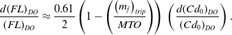 \begin{align}\frac{{d{{\left( {FL} \right)}_{DO}}}}{{{{\left( {FL} \right)}_{DO}}}} \approx \frac{{0.61}}{2}\left( {1 - \left( {\frac{{{{\left( {{m_f}} \right)}_{trip}}}}{{MTO}}} \right)} \right)\;\left( {\frac{{d{{\left( {C{d_0}} \right)}_{DO}}}}{{{{\left( {C{d_0}} \right)}_{DO}}}}} \right).\end{align}
Since the ratio of trip fuel mass to take-off mass can never exceed unity, all other things being equal, a decrease in Cd 0 always lowers the optimum cruise flight level.


 Open access