

1. Introduction
The aim of the present work is to discuss the thermo-mechanical behaviour of the lithosphere of the Alps and Northern Apennines during the transition from continental rifting to oceanization of the Alpine Tethys.
After the Variscan Orogeny, the future Alpine area (Fig. 1) underwent an extensional stage leading to the break-up of the Pangaea continental lithosphere and the opening of the Alpine Tethys Ocean (Lardeaux & Spalla, Reference Lardeaux and Spalla1991; Diella, Spalla & Tunesi, Reference Diella, Spalla and Tunesi1992; Dal Piaz, Reference Dal Piaz, Raumer and Neubauer1993; Bertotti et al. Reference Bertotti, Picotti, Bernoulli and Castellarin1993; Handy et al. Reference Handy, Franz, Heller, Janott and Zurbriggen1999; Schuster et al. Reference Schuster, Scharbert, Abart and Frank2001; Schuster & Stüwe, Reference Schuster and Stüwe2008; Marotta, Spalla & Gosso, Reference Marotta, Spalla, Gosso, Ring and Wernicke2009). The influence of the thermal, structural and compositional inheritance of the Variscan collision and collapse on the following extensional stage is still under debate (e.g. Marotta & Spalla Reference Marotta and Spalla2007; Von Raumer et al. Reference von Raumer, Bussy, Schaltegger, Schulz and Stampfli2013; Spalla et al. Reference Spalla, Zanoni, Marotta, Rebay, Roda, Zucali, Gosso, Schulmann, Martínez Catalán, Lardeaux, Janoušek and Oggiano2014).
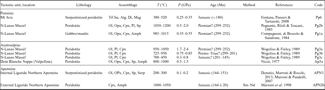
Tectonic map of the Alps and Apennines (after Marotta & Spalla, Reference Marotta and Spalla2007; Handy et al. Reference Handy, Schmid, Bousquet, Kissling and Bernoulli2010) with the locations of: metamorphic rocks and main gabbro bodies of Permian–Triassic age occurring in the pre-Alpine continental crust of the Alps; and mantle rocks and oceanic gabbros from the Alps and Northern Apennines. The codes are defined in Tables 2–5.

The thermal structure of the Alpine lithosphere before the rifting event is poorly understood. Based on petrological analyses of the Ivrea crustal section, Handy et al. (Reference Handy, Franz, Heller, Janott and Zurbriggen1999) and Smye & Stockli (Reference Smye and Stockli2014) proposed that a series of thermal pulses after Carboniferous time affected the pre-rifting Alpine crust, potentially associated with and following the asthenosphere upwelling driven by hyperextension of the Adriatic margin during Late Triassic – Early Jurassic time. According to recent interpretations, the elevated temperatures in the deep crust of the Ivrea Zone may persist for millions of years, remaining close to the solidus for approximately 30 Ma (Klötzli et al. Reference Klötzli, Sinigoi, Quick, Demarchi, Tassinari, Sato and Günes2014) and thermally perturbing the Alpine lithosphere before the beginning of the rifting. Passive extension in the Europa-Adria system is thought to have been active during Triassic time (Handy & Zingg, Reference Handy and Zingg1991; Muntener, Hermann & Trommsdorf, Reference Muntener, Hermann and Trommsdorf2000; Muntener & Hermann, Reference Muntener, Hermann, Wilson, Whitmarsh, Taylor and Froitzheim2001; Montanini, Tribuzio & Anczkiewicz, Reference Montanini, Tribuzio and Anczkiewicz2006) or to have started during late Palaeozoic time (Lardeaux & Spalla, Reference Lardeaux and Spalla1991; Diella, Spalla & Tunesi, Reference Diella, Spalla and Tunesi1992; Dal Piaz, Reference Dal Piaz, Raumer and Neubauer1993; Marotta & Spalla, Reference Marotta and Spalla2007; Marotta, Spalla & Gosso, Reference Marotta, Spalla, Gosso, Ring and Wernicke2009). In contrast, based on data from Val Malenco, Corsica, Erro-Tobbio and Voltri Massif, Piccardo, Padovano & Guarnieri (Reference Piccardo, Padovano and Guarnieri2014) proposed that the pre-rift mantle lithosphere was equilibrated along an intermediate subcontinental geothermal gradient and the Permian high-temperature event(s) was followed by isobaric cooling, lasting more than 50 Ma (Manatschal, Reference Manatschal2004). This interpretation suggests the occurrence of a thermally equilibrated lithosphere before the rifting event (Lavier & Manatschal, Reference Lavier and Manatschal2006). This idea is supported by numerous rifting models proposed for the Alpine area (e.g. Beltrando, Rubatto & Manatschal, Reference Beltrando, Rubatto and Manatschal2010; Mohn et al. Reference Mohn, Manatschal, Beltrando, Masini and Kusznir2012) that were conceived based exclusively on data from the exploration of the Iberia passive margin (e.g. Boillot, Beslier & Girardeau, Reference Boillot, Beslier, Girardeau, Banda, Torné and Talwani1995; Hébert et al. Reference Hébert, Beaudoin, Rochon and Gardien2008).
Numerous numerical and analogue models of continental extension highlight the roles of different parameters and mechanisms in dictating the final geometry and style of the rifting and continental break-up. Among others, Reston & Morgan (Reference Reston and Morgan2004), Van Avendonk et al. (Reference Van Avendonk, Lavier, Shillington and Manatschal2009), Brune & Autin (Reference Brune and Autin2013) and Brune et al. (Reference Brune, Heine, Pérez-Gussinyé and Sobolev2014) focus on the role of the thermal state of the lithosphere; Buck (Reference Buck1991), Corti et al. (Reference Corti, Bonini, Sokoutis, Innocenti, Manetti, Cloetingh and Mulugeta2004), Nagel & Buck (Reference Nagel and Buck2004), Huismans, Buiter & Beaumont (Reference Huismans, Buiter and Beaumont2005), Huismans & Beaumont (Reference Huismans and Beaumont2011, Reference Huismans and Beaumont2014), Cloetingh et al. (Reference Cloetingh, Burov, Matenco, Beekman, Roure and Ziegler2013), Brune et al. (Reference Brune, Heine, Pérez-Gussinyé and Sobolev2014) and Liao & Gerya (Reference Liao and Gerya2015) analyse the effects of the composition, rheology and strength of the lower crust; Brune (Reference Brune2014) and Brune et al. (Reference Brune, Heine, Pérez-Gussinyé and Sobolev2014) investigate the role of the extensional velocity; Manatschal, Lavier & Chenin (Reference Manatschal, Lavier and Chenin2015) and Naliboff & Buiter (Reference Naliboff and Buiter2015) examine the role of structural and compositional inheritance of the system; and Escartín, Hirth & Evans (Reference Escartín, Hirth and Evans1997) and Pérez-Gussinyé et al. (Reference Pérez-Gussinyé, Reston, Phipps Morgan, Wilson, Whitmarsh, Taylor and Froitzheim2001, Reference Pérez-Gussinyé, Morgan, Reston and Ranero2006) focus on serpentinization. However, these works are not strictly focused on the opening of the Alpine Tethys and do not perform systematic comparisons between the model predictions and the natural data from the continental and oceanic crust of the Alps and Northern Apennines, including P–T estimates, radiometric ages and lithological affinity.
This work represents an advancement of the work of Marotta, Spalla & Gosso (Reference Marotta, Spalla, Gosso, Ring and Wernicke2009) in which a rifting process following a continental collision and ending before the break-up of the continental crust is modelled. They implemented a bi-dimensional numerical geodynamic model to analyse the effects of an active extension during the Permian–Triassic period (300–220 Ma), assuming that the extension developed in a lithosphere already thermally and mechanically perturbed by a previous subduction-collision phase which occurred during the Variscan age, up to 300 Ma. Marotta, Spalla & Gosso (Reference Marotta, Spalla, Gosso, Ring and Wernicke2009)’s results supported the idea of an asymmetric rifting in which the Adriatic continental crust represented the hanging wall, although satisfactory and complete agreement with the natural geological data in terms of the coincidence of age, lithology and P–T values was only obtained at the higher rate of forced extension (2 cm a−1).
Indeed, Marotta, Spalla & Gosso (Reference Marotta, Spalla, Gosso, Ring and Wernicke2009)’s model has two main limits: (a) the model does not evolve until the continental lithosphere break-up and subsequent ocean spreading; and (b) the conditions favourable to mantle partial melting have not been considered; the timing of the beginning of the new oceanic lithosphere was therefore not predicted. For these reasons, in the present work the transition from continental rifting to ocean spreading has been investigated using a two-dimensional (2D) thermo-mechanical numerical model in which the serpentinite formation due to the hydration of the upraising peridotite has been implemented and extension occurs over a mechanically unperturbed lithosphere. The predictions of the model have been compared with natural data related to the Permian–Triassic high-temperature – low-pressure (HT-LP) metamorphism affecting the continental lithosphere and data from the pre-Alpine Jurassic P–T evolution of the oceanic crust from the Alps and the Northern Apennines.
2. Numerical model
2.a. Model set-up
To simulate the transition from rifting to oceanic spreading, a time-dependent 2D thermo-mechanical numerical model has been used in which the dynamics of the crust–mantle system have been investigated by numerical integration of the three fundamental equations of conservation of mass, momentum and energy:
 $$\begin{equation}
\nabla \cdot \vec{u} & =& 0\\
\end{equation}$$
$$\begin{equation}
\nabla \cdot \vec{u} & =& 0\\
\end{equation}$$
 $$\begin{equation}- \nabla P + \nabla \cdot \vec{\tau } + \rho \vec{g} & =& 0\\
\end{equation}$$
$$\begin{equation}- \nabla P + \nabla \cdot \vec{\tau } + \rho \vec{g} & =& 0\\
\end{equation}$$
 $$\begin{equation}
\rho {c_p}\left( {\frac{{\partial T}}{{\partial t}} + \vec{u} \cdot \nabla T} \right) & =& \nabla \cdot \left( {K\nabla T} \right) + \rho {H_d}
\end{equation}$$
$$\begin{equation}
\rho {c_p}\left( {\frac{{\partial T}}{{\partial t}} + \vec{u} \cdot \nabla T} \right) & =& \nabla \cdot \left( {K\nabla T} \right) + \rho {H_d}
\end{equation}$$
respectively, where $\vec{u}$
is the velocity, P is the pressure,
$\vec{u}$
is the velocity, P is the pressure, $\vec{\tau }$
is the deviatoric stress, ρ is the density,
$\vec{\tau }$
is the deviatoric stress, ρ is the density, $\vec{g}$
is the gravity acceleration, cp
is the specific heat at constant pressure, T is the temperature, K is the thermal conductivity and Hd
is the radiogenic heat production rate per unit mass.
$\vec{g}$
is the gravity acceleration, cp
is the specific heat at constant pressure, T is the temperature, K is the thermal conductivity and Hd
is the radiogenic heat production rate per unit mass.
Equations (1), (2) and (3) are solved using the 2D finite-elements code SubMar, which has been exhaustively described by Marotta, Spelta & Rizzetto (Reference Marotta, Spelta and Rizzetto2006). This numerical code uses the penalty function formulation to integrate the equation for the conservation of momentum and the streamline upwind/Petrov-Galerkin method to integrate the equation for the conservation of energy.
The marker in-cell technique has been used to compositionally differentiate crust and mantle rocks.
A viscous-plastic behaviour has been assumed for both materials. The effective viscosity is calculated as follows:
 $$\begin{equation}
{\mu ^{{\rm{eff}}}} = {\mu _{{\rm{viscous}}}} = {\mu _{0,i}}\exp\left[ {\frac{{{E_i}}}{R}\left( {\frac{1}{T} - \frac{1}{{{T_0}}}} \right)} \right]
\end{equation}$$
$$\begin{equation}
{\mu ^{{\rm{eff}}}} = {\mu _{{\rm{viscous}}}} = {\mu _{0,i}}\exp\left[ {\frac{{{E_i}}}{R}\left( {\frac{1}{T} - \frac{1}{{{T_0}}}} \right)} \right]
\end{equation}$$
where μ 0, i and Ei are the reference viscosity at the reference temperature T 0 and the activation energy for the crust (i = c) and the mantle (i = m), respectively, with a maximum value defined by the plastic viscosity assumed equal to 1025 Pa s (Table 1).
Material properties used in the 2-D numerical modelling

a Dubois & Diament (Reference Dubois and Diament1997) and Best & Christiansen (Reference Best and Christiansen2001); bRybach (Reference Rybach, Haenel, Stegena and Rybach1988); cRanalli & Murphy (Reference Ranalli and Murphy1987); dChopra & Peterson (Reference Chopra and Peterson1981); eHonda & Saito (Reference Honda and Saito2003), Arcay, Tric & Doin (Reference Arcay, Tric and Doin2005) and Roda, Marotta & Spalla (Reference Roda, Marotta and Spalla2010).
We account for a brittle behaviour of the crust to define the rheological conditions for mantle serpentinization only, as better specified in Section 2.b.
The material parameters are listed in Table 1. Initially, the lithosphere is mechanically unperturbed and laterally homogeneous. The initial thickness of the continental crust is assumed to be 30 km (Fig. 2), which is in agreement with models envisaging the beginning of extension-transtension onto a lithosphere characterized by a crust with a thickness of approximately 30 km (Muntener, Hermann & Trommsdorf, Reference Muntener, Hermann and Trommsdorf2000; Manatschal, Reference Manatschal2004).
(a) 2D geometry and numerical set-up of the model. (b) Thermal and rheological profiles at the beginning of the evolution for the hot (red lines) and cold (blue lines) models. The solid lines indicate the effective viscosity profiles, corresponding to the geotherms indicated by the dashed lines.
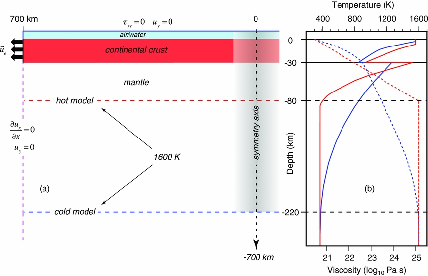
Two thermal settings are proposed here to satisfy two contrasting pre-rifting settings of the Alpine lithosphere characterized by different depths of the 1600 K isotherm: 80 and 220 km (Fig. 2b). We refer to these simulations as the hot and cold models, respectively. The initial thermal conditions correspond to an almost conductive thermal profile from 300 K at the surface to 1600 K at the base of the lithosphere; an initial homogeneous temperature of 1600 K is assumed below the lithosphere (Fig. 2b).
Boundary conditions are defined in terms of the temperature and velocity. A temperature of 300 K is fixed at the top of the crust and throughout the air–water layer, a temperature of 1600 K is fixed at the base of the model and zero flux is assumed through the lateral sides of the model. We apply an extension rate of 1.25 cm a−1 at both lateral sides of the model throughout the crustal thickness, resulting in a symmetric passive rifting with a total extension rate of 2.5 cm a−1, compatible with the magma-poor nature of the rift (e.g. Manatschal & Müntener, Reference Manatschal and Müntener2009). The 2D domain is closed vertically with shear-free conditions prescribed along the top and the bottom of the model domain, while both crust and lithospheric mantle are allowed to exit the model boundaries allowing the thinning of either crust and lithospheric mantle (Fig. 2a).
Considering that in the Alpine literature the onset of rifting is proposed to occur during 220–200 Ma (Müntener, Hermann & Trommsdorf, Reference Muntener, Hermann and Trommsdorf2000; Manatschal, Reference Manatschal2004; Montanini, Tribuzio & Anczkiewicz, Reference Montanini, Tribuzio and Anczkiewicz2006; Piccardo, Padovano & Guarnieri, Reference Piccardo, Padovano and Guarnieri2014) and that the oldest rocks of the ophiolitic associations belonging to the Liguria–Piemonte Ocean have been dated at 175–160 Ma (Tribuzio, Thirwall & Vannucci, Reference Tribuzio, Thirwall and Vannucci2004; Rossi et al. Reference Rossi, Lahondère, Cocherie, Caballero and Féraud2012; Kaczmarek, Müntener & Rubatto, Reference Kaczmarek, Müntener and Rubatto2008; Li et al. Reference Li, Faure, Lin and Manatschal2013, Reference Li, Faure, Rossi, Lin and Lahondère2015), we run the simulation over a time span of 60 Ma to match the time interval needed to generate the oldest gabbro intrusions in the natural system.
2.b. Conditions for mantle serpentinization
Magmatic-poor margins formed by the rifting of continental crust are characterized by the occurrence of serpentinized peridotites within a broad continent-ocean transition (e.g. Pérez-Gussinyé et al. Reference Pérez-Gussinyé, Reston, Phipps Morgan, Wilson, Whitmarsh, Taylor and Froitzheim2001; Manatschal, Reference Manatschal2004) and by the lithostratigraphy of the ophiolitic sequences (Mevel, Caby & Kienast, Reference Mevel, Caby and Kienast1978; Lagabrielle & Cannat, Reference Lagabrielle and Cannat1990; Chalot-Prat, Reference Chalot-Prat, Foulger, Natland, Presnall and Anderson2005; Manatschal et al. Reference Manatschal, Sauter, Karpoff, Masini, Mohn and Lagabrielle2011; Li et al. Reference Li, Faure, Lin and Manatschal2013). The role of serpentinization of the lithospheric mantle during continental rifting and the transition to oceanic spreading has been extensively discussed by Pérez-Gussinyé et al. (Reference Pérez-Gussinyé, Reston, Phipps Morgan, Wilson, Whitmarsh, Taylor and Froitzheim2001, Reference Pérez-Gussinyé, Morgan, Reston and Ranero2006). They assume that mantle serpentinization occurs when the overlaying crustal layer is under brittle conditions, so that faults can cut across the crust allowing hydrous fluids to penetrate the mantle, and mantle matches the appropriate pressure and temperature conditions for the stability field of serpentine.
In order to implement mantle serpentinization and the consequent rheological and compositional changes, we check whether the pressure and temperature of each mantle-type marker match the stability field of serpentine and the overlying crustal layer is under brittle conditions. To define whether the overlying layer is under brittle conditions, we use a simplified formulation of Byerlee's law criterion:
 $$\begin{equation}
{\sigma _{{\rm{brittle}}}} = \beta \cdot y\quad \quad {\rm{with}}\quad \quad \beta = 16\;{\rm{MPa}}\;{\rm{k}}{{\rm{m}}^{ - 1}}
\end{equation}$$
$$\begin{equation}
{\sigma _{{\rm{brittle}}}} = \beta \cdot y\quad \quad {\rm{with}}\quad \quad \beta = 16\;{\rm{MPa}}\;{\rm{k}}{{\rm{m}}^{ - 1}}
\end{equation}$$
where y is the depth, and compare the brittle strength σbrittle with the temperature- and pressure-based plastic strength:
 $$\begin{equation}
{\rm{Regime}} \Leftarrow \min \left\{ {{\sigma _{{\rm{brittle}}}},{\sigma _{{\rm{plastic}}}}} \right\}.
\end{equation}$$
$$\begin{equation}
{\rm{Regime}} \Leftarrow \min \left\{ {{\sigma _{{\rm{brittle}}}},{\sigma _{{\rm{plastic}}}}} \right\}.
\end{equation}$$
2.c. Conditions for partial melting
During an active extension of a continental lithosphere, the temperature in the lithospheric mantle increases as a consequence of the upwelling asthenospheric flow. If the pressure and temperature conditions of peridotite solidus are matched, partial melting of the lithospheric mantle occurs and gabbroic-basaltic melts form. We assume here that once the mantle partial melting occurs in the system, the oceanic lithosphere starts to form. This implies an instantaneous transfer of the mantle melt to the surface in agreement with the estimates of the rate of magma ascent across the continental and oceanic crust (Clague, Reference Clague1987; Turner et al. Reference Turner, George, Evans, Hawkesworth and Zellmer2000).
In order to individuate the beginning of oceanic spreading and to identify the extension of the partially molten mantle region, we check the pressure and temperature conditions of each mantle-type marker during the evolution. When the P–T conditions reach the dry solidus field of peridotite (Rogers et al. Reference Rogers, Blake, Widdowson, Parkinson and Harris2008):
 $$\begin{equation}
{P_{\rm{m}}} \le \alpha \cdot {T_{\rm{m}}} + \beta ,
\end{equation}$$
$$\begin{equation}
{P_{\rm{m}}} \le \alpha \cdot {T_{\rm{m}}} + \beta ,
\end{equation}$$
where α = 0.00789792857 GPa K−1 and β = – 11.1071202 GPa, its typology is changed from mantle type into potential partially molten mantle type.
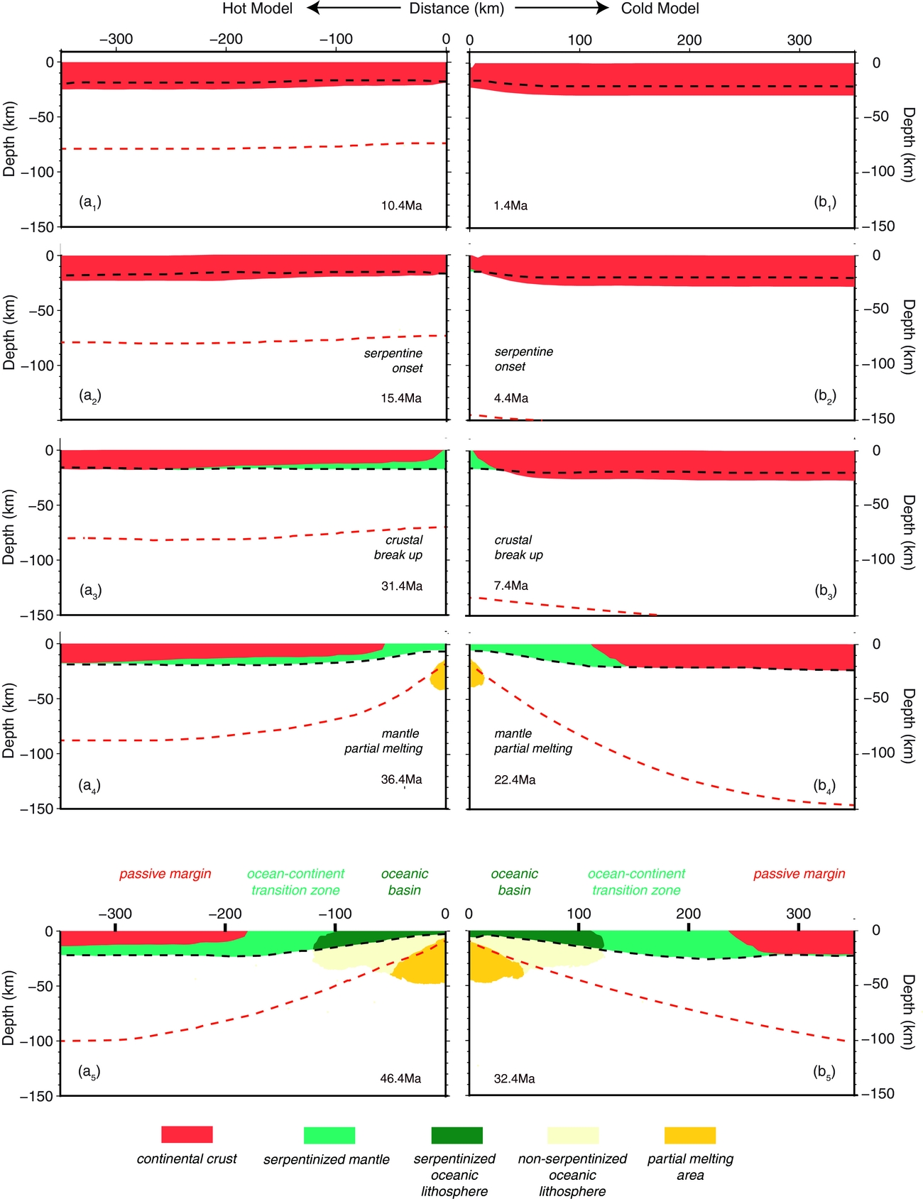
The extension of the partially molten mantle region is shown in Figure 3 distinguishing the oceanic lithosphere (dark green), formed by serpentinized mantle hosting gabbros and basalts that can be produced once partial melting conditions are attained, from the mantle that serpentinized before the occurrence of partial melting (light green).
Successive stages of the tectonic evolution predicted by the hot (panels ai) and cold (panels bi) models at different times after the beginning of the forced extension. Black and red dashed lines correspond to 800 K and 1500 K isotherms, respectively. Ages refer to the time span from the beginning of the simulations.
In the present form, the compositional and rheological changes consequent to partial melting are not implemented.
3. Model predictions
3.a. Structural configurations
Figure 3 shows the structural configurations of the crust and lithosphere at different stages of the evolution of the hot model (panels ai, left side) and the cold model (panels bi, right side). The crustal boundaries coincide with the envelope of the crustal type markers. The base of the lithosphere is thermally defined by the 1600 K isotherm (red dashed line).
During the initial phase of forced extension in both models a progressive thinning of the crust is predicted, mostly concentrated around the position of the future ridge. The crustal thinning occurs very early in the cold model, approximately 1 Ma after the beginning of the extension (Fig. 3b1), while more than 10 Ma passes before thinning becomes significant in the hot model (Fig. 3a1). After 15.4 Ma (hot model, Fig. 3a2) and 4.4 Ma (cold model, Fig. 3b2), the thermal thinning is localized around the position of the future ridge. These times mark the beginning of mantle serpentinization in both models. The long time interval necessary in the hot model for the beginning of deformation localization therefore seems related to the higher thermal state at the base of the continental crust, which results in a different rheological behaviour of the shallow lithospheric mantle as discussed at the end of Section 2.c.
The progression of forced extension leads to the occurrence of the crustal break-up which occurs at 31.4 Ma in the hot model, approximately 16 Ma after the beginning of the mantle serpentinization (Fig. 3a3), and at 7.4 Ma in the cold model, only 3 Ma after the beginning of the mantle serpentinization (Fig. 3b3). The occurrence of crustal break-up is followed by the exhumation of the serpentinized mantle replacing the thinned continental crust at the floor of the basin. In the hot model, the mantle serpentinization progresses even at the base of the continental crust for more than 250 km away from the ridge. In contrast, in the cold model deep-seated serpentinization does not occur. This is a consequence of the thinner continental crust characterizing the hot model, allowing the occurrence of mantle at shallower depths with respect to the cold model in which continental lithospheric mantle resides at greater depths and P–T conditions are inappropriate for serpentinization.
The pressure and temperature conditions at the base of the lithosphere in the hot model are favourable for partial melting for a relatively short time after the crustal break-up (approximately 5 Ma, Fig. 3a4). In contrast, in the cold model favourable pressure and temperature conditions are reached after a relatively long time from the break-up (approximately 15 Ma, Fig. 3b4). Although there are different time intervals between the different stages (thinning, serpentinization and partial melting) in the hot and cold models, once crustal thinning starts comparable time spans pass before the beginning of the mantle partial melting in both models (approximately 21 Ma and 18 Ma for the hot and the cold models, respectively; Fig. 4).
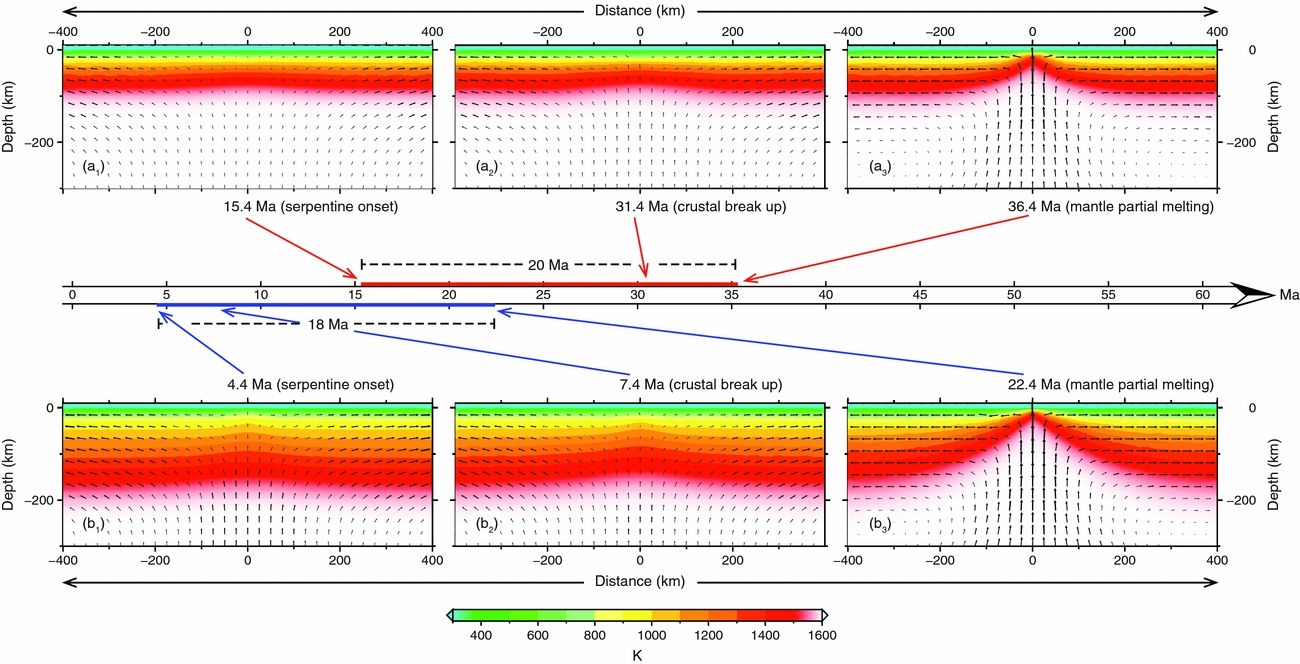
Thermal and velocity fields of the system at different times after the beginning of the forced extension for the hot (panels ai) and cold (panels bi) models. Time scale in the centre of the figure represents the simulation duration for both models, on which the onset of serpentinization, crustal break-up and partial melting are located by arrows (red for the hot and blue for the cold models). Time intervals between serpentinization and partial melting onset are indicated by dashed lines.
At the beginning of the extension, the low strength of the lithosphere in the hot model reduces the efficiency of stress transmission up to shallow depths, making the localization of crustal thinning slower than that for the stronger lithosphere of the cold model. Once the crustal thinning is localized, the successive evolution is dominated by local thermal gradients because this stage is comparable in the two models. After their formation, the mantle, which is depleted by partial melting (dark yellow markers for the partial melting area and light yellow markers for the depleted mantle in Fig. 3a5, b5), moves laterally below the expanding oceanic crust, forming the oceanic lithosphere (dark green markers in Fig. 3a5, b5).
Surface horizontal crustal velocity predicted by the hot (a) and cold (b) models at different times after the beginning of the forced extension.
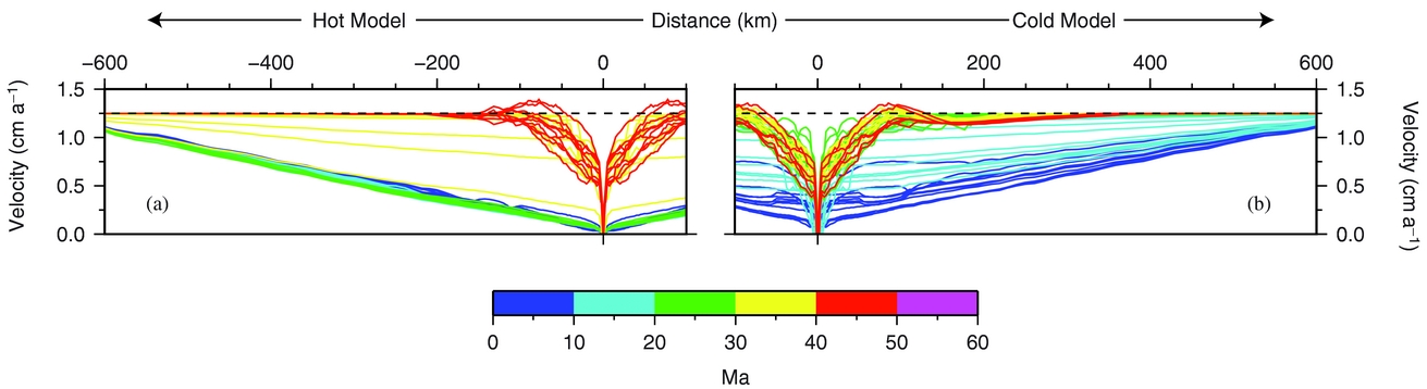
Here we assume that the oceanic lithosphere forms after the beginning of the mantle partial melting, when gabbros, basalts and part of serpentinized mantle contribute to the formation of the oceanic crust. Based on the structural configuration of the system at the time of partial melting (Fig. 3a4, b4) and after a given time span of 10 Ma (Fig. 3a5 and b5 for the hot model and the cold model, respectively), it is possible to estimate the variation in time of the width of the oceanic lithosphere, characterized by a gabbro-basalt-bearing crust, and of the serpentinized mantle denuded before melt generation. In particular, 10 Ma after the onset of the mantle partial melting our results indicate a total basin width ranging over 360–480 km as a function of the initial thermal state of the lithosphere (hot or cold models, respectively). In both models the oceanic lithosphere extends for approximately 200 km, while the denuded serpentinized mantle covers a width of approximately 160 km in the hot model and 280 km in the cold one.
3.b. Thermo-mechanical evolution
The structural configuration discussed above can be better understood if the thermo-mechanical evolution of the system is analysed. Figure 4 shows the thermal and velocity fields of the system at different stages of the evolution for the hot and the cold models (Fig. 4ai and bi, respectively). During the early stages of the evolution of both models, the velocity field is controlled by the far-field traction driving a predominantly horizontal velocity pattern though the lithosphere, being the intensity of the mantle upwelling below the future ridge lower than half the intensity of the far-field for the cold model (panel b1) and even negligible for the hot model (panel a1). Mantle upwelling increases during the evolution (Fig. 4a2) and reaches a magnitude comparable to or higher than that of the far-field traction only after the onset of the mantle partial melting (Fig. 4a3). For both models, the thermal thinning of the lithosphere localizes at the future ridge position when the mantle serpentinization conditions are matched, at approximately 15 Ma (Fig. 4a1) and 4.4 Ma (Fig. 4b1) after the beginning of the forced extension for the hot and cold models, respectively. Thermal thinning achieves its maximum when the pressure and temperature conditions are favourable for the mantle partial melting at 36.4 Ma (Fig. 4a3) and 22.4 Ma (Fig. 4b3) for the hot and cold models, respectively. The thermal thinning in the two models therefore differs only in the initial stages and, once the thermal destabilization starts, the time span needed to reach the maximum thinning is approximately independent of the initial thermal state (thick red and blue lines along the time scale in Fig. 4).
The different behaviours of the cold and hot models during the initial deformation phase and their similar behaviours at longer times can be ascribed to the differences in the lithosphere strength (Fig. 2b). During the initial phase, the lower strength (in terms of the lower effective viscosities of the lithospheric mantle levels) that characterizes the hot model (solid red line in Fig. 2b) may attenuate the transmission of the far-field traction up to the future ridge position, making the lithosphere thinning a very slow process compared with the cold model.
3.c. Velocity configuration
A more detailed analysis of the surface crustal horizontal velocity (Fig. 5a, b) indicates that both models are characterized by an initial phase during which the mean surface crustal velocity is stationary and increases linearly from the future ridge outwards until it reaches, at the boundary of the model, the velocity value constrained by the far-field traction. This stationary pattern lasts a short time (approximately 5 Ma) in the cold model (Fig. 5a) and a long time (approximately 30 Ma) in the hot model (Fig. 5b), ending when the crustal break-up occurs. This initial phase is followed by a transition phase lasting approximately 9 Ma and 3 Ma for the cold and hot models, respectively, during which the far-field and upwelling flow concur to the extension rate and the mean surface crustal horizontal velocities progressively increase until they reach the value of the far-field traction velocity. At the advanced stages of evolution the surface crustal horizontal velocity remains almost constant from the ridge to the margins for both models, with the exception of a 150–200 km wide region around the ridge where the mean surface horizontal velocity of the crust is mainly controlled by the very intense mantle upwelling flow and may overcome the far-field value.
The transmission of the spreading rate towards the periphery of the domain is likely limited by the fixed far-field prescribed velocity at the boundaries of the model producing, at first sight, an artificial local shortening.
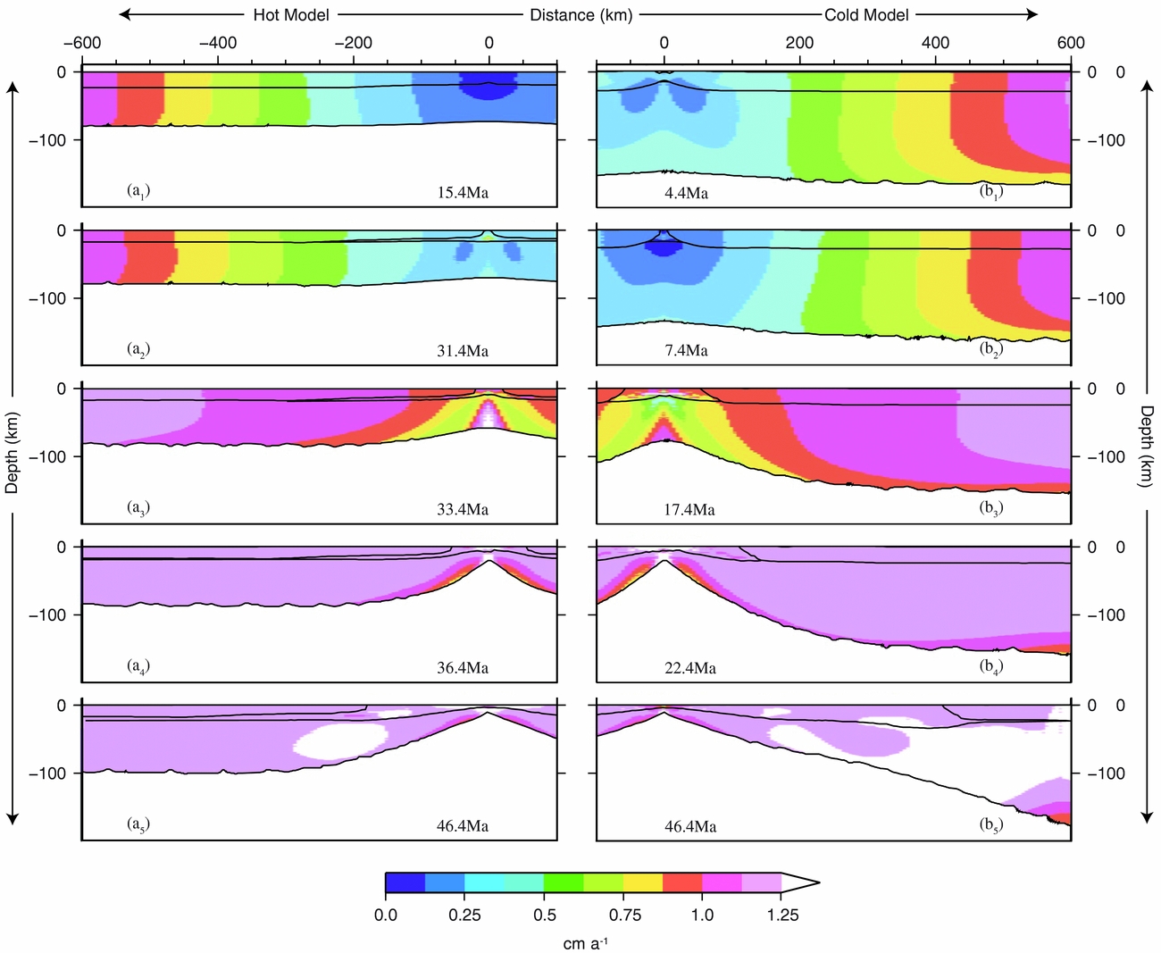
Figure 6 shows the maps of the velocity modules through the lithospheric thickness at different time steps of the evolution, for the hot (Fig. 6ai) and cold (Fig. 6bi) models. Until crustal break-up occurs, the linear increase from the ridge outwards observed in the mean surface crustal velocity (Fig. 5) characterizes the entire lithosphere thickness (Fig. 6a1, a2 for the hot model and Fig. 6b1, b2 for the cold model). A small increase in the velocity is evident within the mantle where a decrease in the viscosity occurs because of the serpentinization. After the crustal break-up, the strongest velocity gradients localize within 200 km around the ridge and are associated with the increase in the magnitude of the upwelling mantle flow (Fig. 4). In the proximity of the ridge, in both models the extension rate at the base of the crust increases by a factor of 2–4 since the continental break-up to oceanic spreading (compare Fig. 6a2, b2 to Fig. 6a3, b3). Further away, the velocity gradients decrease significantly until they disappear, and the entire continental lithosphere moves as a rigid plate at a rate equal to the traction velocity after the onset of the mantle partial melting. Significant velocity gradients persist within the part of the basin floored by the serpentinized mantle and at the deep lithosphere levels below the ridge, where the intensity of the asthenosphere upwelling overcomes the far-field traction velocity (compare Fig. 4a3, b3 to Fig. 6a4, b4). At the advanced stages of the evolution after the onset of the mantle partial melting, as already observed in Figure 5 for the mean surface horizontal velocity, even the lithosphere velocity overcomes the far-field traction velocity up to a maximum value of 1.4 cm a−1 compared with the prescribed 1.25 cm a−1.
Maps of the velocity modules throughout the lithosphere at different times after the beginning of the forced extension for the hot (panels ai) and cold (panels bi) models.
4. Natural data
The natural data, compared with the model predictions in the following discussion, are derived from continental and oceanic rocks from the Alps and Apennines and include:
-
1. lithotypes: useful for inferring the continental, oceanic, crustal or mantellic provenance of each considered rock type as well as the raw characterization of the associable lithostratigraphic setting;
-
2. P–T conditions: useful for individuating potential provenance regions along the model-predicted lithospheric cross-sections based on the occurrence of compatible thermal states; and
-
3. geochronological data: useful for checking the time correspondences of the mineral assemblage developments with the predicted sequence of thermal states from rifting to oceanic spreading.
The kinematics of the natural structures supported by mineral assemblages, which are used to infer the considered P–T estimates, are also reported as a supplementary check for compatibility with the investigated lithospheric extensional regime.
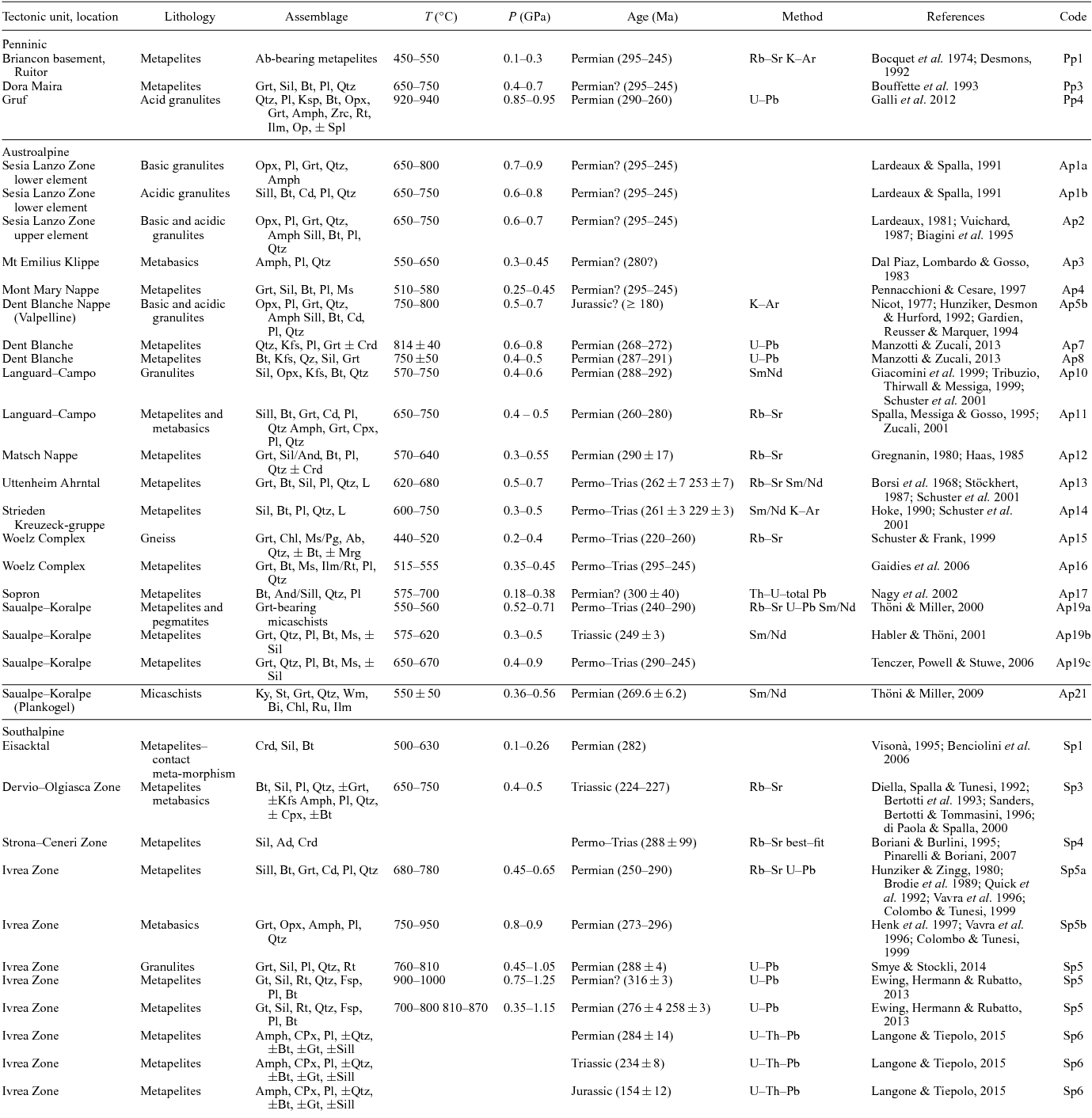
The rock types, mineral assemblages and climax metamorphic conditions are described in Tables 2–5. In the pre-Mesozoic continental lithosphere of the Alps and Apennines, the metamorphic T max imprints and igneous activity compatible with the high thermal regime induced by mantle upwelling during lithospheric thinning have Permian–Triassic ages. These estimated conditions have therefore been selected for comparison with model predictions. On the contrary, the age data from the oceanic lithosphere selected for comparison with model predictions are concentrated around Middle Jurassic ages and are referred to gabbro emplacement and metamorphic re-equilibration at the ocean floor.
A synthetic geological outline is given to help readers who are not familiar with the Alps and Apennines to place the samples that have provided the natural data in an adequate tectonic frame.
4.a. Geological outline
The Alps and Apennines developed during the closure of the Mesozoic Tethys along two opposite subduction zones during different time intervals, during Cretaceous–Oligocene time for the Alpine system and from Eocene time to the present day for the Apennines system (e.g. Dal Piaz, Reference Dal Piaz, Beltrando, Peccerillo, Mattei, Conticelli and Doglioni2010; Handy et al. Reference Handy, Schmid, Bousquet, Kissling and Bernoulli2010; Carminati & Doglioni, Reference Carminati and Doglioni2012). Different erosion percentages and exhumation efficiencies (Carminati & Doglioni, Reference Carminati and Doglioni2012) allowed the exposure of deep structural levels in the axial zone of the Alpine nappe; however, these levels are still buried in the Apennines. In contrast to the Apennines, denudation of the axial part of the belt makes the Alps an important site where it is possible to explore continuous sections of deep and intermediate Alpine and pre-Alpine continental crust and to investigate the metamorphic and igneous effects of the lithospheric-thinning-induced high thermal regime preceding Alpine convergence.
The Alps spread out from the Gulf of Genova to the Vienna Basin; the chain was truncated during the Neogenic opening of the Ligurian–Provençal–Algerian and Tyrrhenian basins (e.g. Bozzo et al. Reference Bozzo, Campi, Capponi and Giglia1992; Séranne, Reference Seranne, Durand, Jolivet, Horvath and Seranne1999; Federico et al. Reference Federico, Spagnolo, Crispini and Capponi2009; Turco et al. Reference Turco, Macchiavelli, Mazzoli, Schettino and Pierantoni2012). Alpine subduction-collision is responsible for the distribution of the continental pre-Alpine and Mesozoic oceanic rocks in four tectonic domains, individuated and explored at the lithospheric scale after the seismic integrated geophysical prospection projects of the whole belt (e.g. Polino, Dal Piaz & Gosso, Reference Polino, Dal Piaz and Gosso1990; Schmid et al. Reference Schmid, Fügenschuh, Kissling and Schuster2004; Cassinis, Reference Cassinis2006). From the internal to the external part of the belt, they are the Southalpine, Austroalpine, Penninic and Helvetic domains (Fig. 1).
The Southalpine domain consists of a south-verging thrust system that has been active since Cretaceous time, involving Palaeozoic continental basement and Permian–Cenozoic cover units, both only locally affected by very-low-grade Alpine metamorphism. The Austroalpine and Penninic domains have been deeply involved in the Alpine subduction and collision system, as accounted for by the high-pressure metamorphic imprints associated with the dominant Alpine fabrics. The Penninic domain consists of mingled crustal slices deriving from both pre-Alpine continental and Mesozoic oceanic lithosphere, the latter tectonically sampled from the subducted Tethys Ocean (e.g. Platt Reference Platt1986; Polino, Dal Piaz & Gosso, Reference Polino, Dal Piaz and Gosso1990; Stöckhert & Gerya, Reference Stöckhert and Gerya2005; Malatesta et al. Reference Malatesta, Crispini, Federico, Capponi and Scambelluri2012; Roda, Spalla & Marotta, Reference Roda, Spalla and Marotta2012; Malatesta et al. Reference Malatesta, Gerya, Crispini, Federico and Capponi2013). In contrast, the Austroalpine domain does not contain Mesozoic ophiolites but is infolded within them and the related Mesozoic sediments all along its external boundary. Finally, the Helvetic domain consists of a Europe-verging thrust system that includes basement and cover slices structured during the late stages of the Alpine continental collision since Tertiary. Due to its shallow-level Alpine tectonic history, the Helvetic and Southalpine units (Fig. 1) broadly preserve pre-Alpine metamorphic, structural and stratigraphic imprints (Fig. 7), whereas Cretaceous–Paleocene Alpine high-pressure rocks are confined within the axial part of the chain in a rootless crustal prism consisting of Penninic and Austroalpine units. These latter are bounded by the Penninic frontal thrust (PF, Fig. 1) towards the European foreland and by the Periadriatic lineament (PL, Fig. 1) towards the Adriatic hinterland (Handy & Oberhänsli, Reference Handy and Oberhänsli2004; Thöni et al. Reference Thöni, Miller, Blichert-Toft, Whitehouse, Konzett and Zanetti2008; Roda, Spalla & Marotta, Reference Roda, Spalla and Marotta2012). According to many authors the wide range of radiometric ages of high-pressure metamorphic imprints (Bousquet et al. Reference Bousquet, Engi, Gosso, Oberhänsli, Berger, Spalla, Zucali and Goffè2004; Goffé et al. Reference Goffé, Schwartz, Lardeaux and Bousquet2004; Handy et al. Reference Handy, Schmid, Bousquet, Kissling and Bernoulli2010; Lardeaux, Reference Lardeaux2014) suggests that they were buried and widely exhumed during subduction of the oceanic lithosphere (European lower plate), accompanied by tectonic erosion of the upper continental plate (Adria) before the onset of continental collision (e.g. Platt Reference Platt1986; Polino, Dal Piaz & Gosso, Reference Polino, Dal Piaz and Gosso1990; Spalla et al. Reference Spalla, Lardeaux, Dal Piaz, Gosso and Messiga1996; Gerya & Stöckhert Reference Gerya and Stöckhert2005; Roda, Marotta & Spalla, Reference Roda, Marotta and Spalla2010; Roda, Spalla & Marotta, Reference Roda, Spalla and Marotta2012; Rubatto et al. Reference Rubatto, Regis, Hermann, Boston, Engi, Beltrando and McAlpine2011). Here, pre-Alpine structural, metamorphic and igneous relics are also preserved even if pervasive Alpine structural and metamorphic reworking shapes them into small-sized and scattered lenses, inhibiting the correlation of pre-Alpine structures at the regional scale.
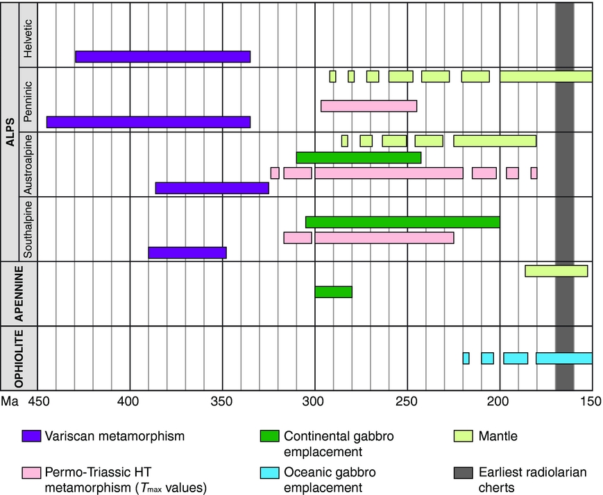
Timing of the metamorphic and magmatic events from Variscan to Jurassic time along the Alpine belt. Radiometric ages are plotted including analytical uncertainty intervals (dashed horizontal bars). Variscan evolutions are synthesized by data in Table 2. Permian–Triassic metamorphic and igneous data (continental gabbros) are synthesized by data in Table 3 and represented with their error margin. Ophiolites and mantle age data are listed in Tables 4 and 5. The grey stripe indicates the age of the earliest radiolarian cherts related to Alpine ophiolites (Cordey & Bailly, Reference Cordey and Bailly2007).
4.b. Lithology, structures, P–T conditions and ages
Asthenospheric upwelling associated with lithospheric thinning causes high thermal regimes in the thinned continental lithosphere (e.g. Thompson, Reference Thompson1981; England & Thompson, Reference England and Thompson1984; Thompson & England, Reference Thompson and England1984; Sandiford & Powell, Reference Sandiford and Powell1986; Spear & Peacock, Reference Spear and Peacock1989; Beardsmore & Cull, Reference Beardsmore and Cull2001), and in the Alps the only igneous and metamorphic effects indicating the occurrence of such a thermal state before the Alpine convergence are of Permian–Triassic age. They are detectable along the whole belt, from the Ligurian Sea to the Pannonian Basin, even in domains strongly reworked by the Alpine tectonics and metamorphism. These records consist of a widespread emplacement of Permian–Triassic basic to acidic igneous activity and huge gabbro bodies (Tables 2 and 3; Fig. 1) associated with regional high-temperature – low-pressure (HT-LP) metamorphism, which postdate structures and metamorphic imprints widely developed during the Variscan subduction and collision (Fig. 7). These features are frequently associated with subcontinental peridotites (Table 4) and are mainly confined to the Austroalpine and Southalpine domains (e.g. Lardeaux & Spalla, Reference Lardeaux and Spalla1991; Bonin et al. Reference Bonin, Brändlein, Bussy, Desmons, Eggenberger, Finger, Graf, Marro, Mercolli, Oberhänsli, Ploquin, Quadt, Raumer, Schaltegger, Steyrer, Visonà, von Raumer and Neubauer1993; Bussy et al. Reference Bussy, Venturini, Hunziker and Martinotti1998; Rottura et al. Reference Rottura, Bargossi, Caggianelli, Del Moro, Visonà and Tranne1998; Schuster et al. Reference Schuster, Scharbert, Abart and Frank2001; Stahle et al. Reference Stahle, Frenzel, Hess, Saupe, Schmidt and Schneider2001; Rebay & Spalla, Reference Rebay and Spalla2001; Rampone, Reference Rampone2002; Peressini et al. Reference Peressini, Quick, Sinigoi, Hofmann and Fanning2007; Marotta, Spalla & Gosso, Reference Marotta, Spalla, Gosso, Ring and Wernicke2009; Spalla et al. Reference Spalla, Zanoni, Marotta, Rebay, Roda, Zucali, Gosso, Schulmann, Martínez Catalán, Lardeaux, Janoušek and Oggiano2014).
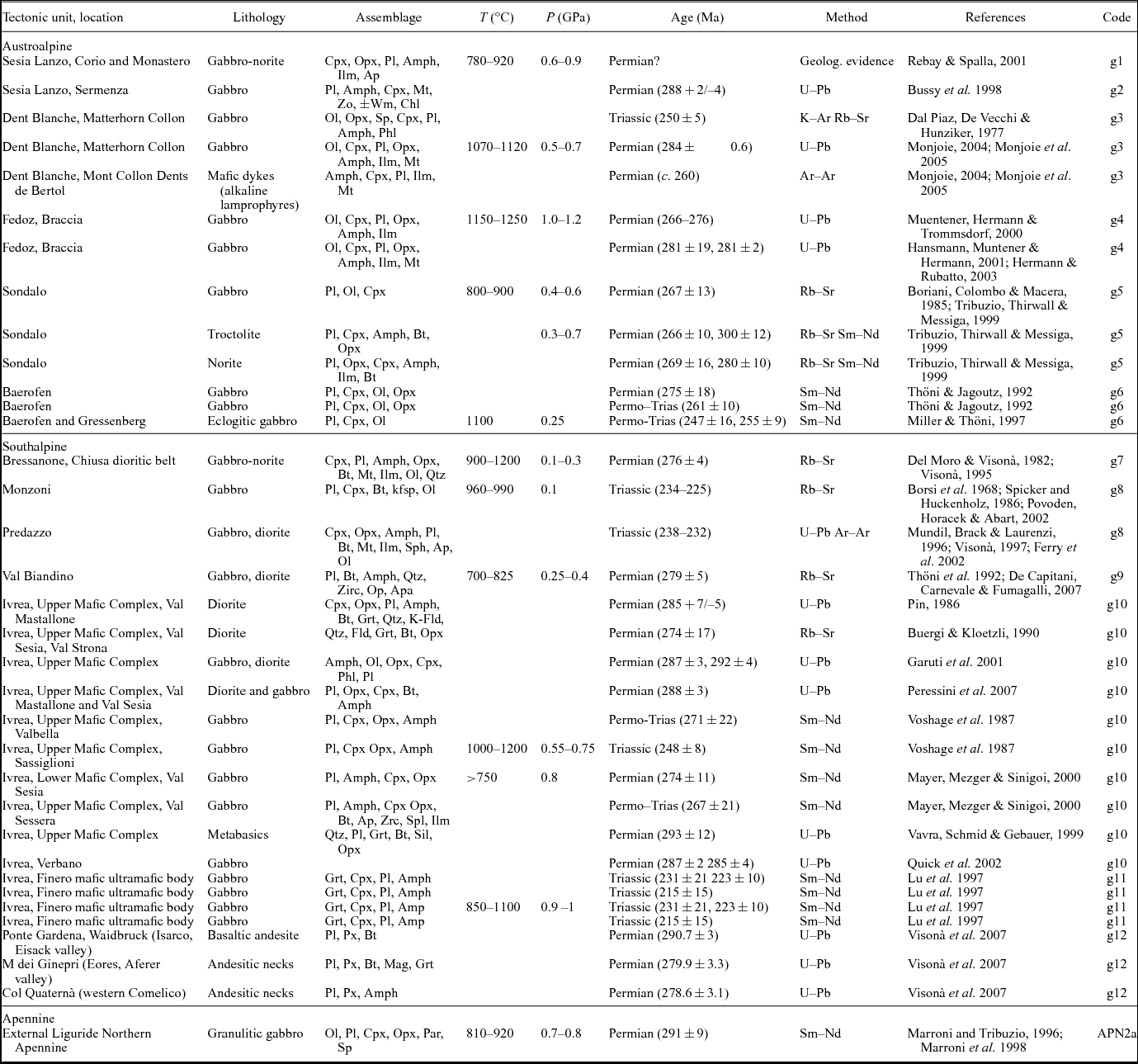
Metamorphic Permian–Triassic imprints are widely recorded in the lower, intermediate and upper continental crust of the Austroalpine and Southalpine domains; only a few records have been recognized in the upper and intermediate Penninic crust of Western Alps, and they are never detected in the Helvetic domain (Fig. 1). In the Penninic domain, HT assemblages mainly developed in sillimanite-bearing metapelites and metaintrusives. They are generally derived from re-equilibration under low-pressure conditions and interpreted as Permian in age (Bouffette, Lardeaux & Caron, Reference Bouffette, Lardeaux and Caron1993; Table 2). Sapphirine-bearing HT- to UHT-IP granulites of the Gruf Complex have been recently petrologically and chronologically investigated, revealing an age of 260–290 Ma for T max conditions (Galli et al. Reference Galli, Le Bayon, Schmidt, Burg, Caddick and Reusser2011). The exhumation of Penninic HT Permian–Triassic rocks was generally associated both with cooling and heating (Desmons, Reference Desmons1992; Bouffette, Lardeaux & Caron, Reference Bouffette, Lardeaux and Caron1993) and occurred before the Alpine convergence, whereas the exhumation of UHT Gruf granulites occurred at the end of the Alpine convergence from the base of the internal European passive margin where they lay since the Permian lithospheric thinning (Galli et al. Reference Galli, Le Bayon, Schmidt, Burg, Caddick and Reusser2011). In the Austroalpine domain, Permian–Triassic HT metamorphism mainly developed in sillimanite- and biotite-bearing gneisses; it is associated with minor mafic granulites, amphibolites and high-grade marbles (Table 2). HT minerals locally mark mylonitic fabrics within discrete shear zones (Lardeaux & Spalla Reference Lardeaux and Spalla1991; Spalla et al. Reference Spalla, Lardeaux, Dal Piaz and Gosso1991), and exhumation paths can be characterized by cooling, heating or isothermal decompression (e.g. Dal Piaz, Lombardo & Gosso, Reference Dal Piaz, Lombardo and Gosso1983; Stöckhert, Reference Stöckhert1987; Vuichard, Reference Vuichard1987; Lardeaux & Spalla, Reference Lardeaux and Spalla1991; Spalla, Messiga & Gosso, Reference Spalla, Messiga and Gosso1995; Schuster et al. Reference Schuster, Scharbert, Abart and Frank2001; Manzotti & Zucali, Reference Manzotti and Zucali2013). Locally, the exhumation was accomplished up to very shallow structural levels (e.g. Rebay & Spalla, Reference Rebay and Spalla2001), suggesting that some Austroalpine units belonged to a thinned continental crust before being subducted during Cretaceous convergence. In the Southalpine basement, Permian–Triassic HT metamorphism developed in metapelites, mafic granulites, amphibolites and high-grade marbles and mainly re-equilibrated under granulite-amphibolite-facies conditions (Table 2). HT paragenesis marks a pervasive foliation that is locally mylonitic within up to kilometre-thick discrete shear zones that are often steepened by Alpine thrusting (e.g. Bertotti et al. Reference Bertotti, Picotti, Bernoulli and Castellarin1993; Gosso, Siletto & Spalla, Reference Gosso, Siletto and Spalla1997). Mylonitic belts developed under upper amphibolite-granulite- to greenschist-facies conditions are widespread in the central Southalpine domain, accounting for regional-scale pervasive extensional tectonics (Brodie, Rex & Rutter, Reference Brodie, Rex, Rutter, Coward, Dietrich and Park1989; Diella, Spalla & Tunesi, Reference Diella, Spalla and Tunesi1992; Bertotti et al. Reference Bertotti, Picotti, Bernoulli and Castellarin1993) and widely interpreted as related to regional-scale normal faults responsible for the exhumation of HT-LP complexes (e.g. Brodie, Rex & Rutter, Reference Brodie, Rex, Rutter, Coward, Dietrich and Park1989; Handy et al. Reference Handy, Franz, Heller, Janott and Zurbriggen1999) during a continuous evolution from Permian to Triassic or Jurassic time (e.g. Bertotti et al. Reference Bertotti, Picotti, Bernoulli and Castellarin1993). Intrusive stocks emplaced at shallow levels during Permian – Early Triassic time are associated with metamorphic aureoles (Povoden, Horacek & Abart, Reference Povoden, Horacek and Abart2002; Benciolini et al. Reference Benciolini, Poli, Visona and Zanferrari2006; Gallien, Abart & Wyhlidal, Reference Gallien, Abart and Wyhlidal2007). Exhumation paths were characterized by cooling or by increasing temperature during decompression (e.g. Brodie, Rex & Rutter, Reference Brodie, Rex, Rutter, Coward, Dietrich and Park1989; di Paola & Spalla Reference di Paola and Spalla2000) and were generally accomplished under a high thermal regime. HT Permian–Triassic mineral associations have never been detected in the pebbles of Permian conglomerates from the Orobic Alps, suggesting that HT rocks were not yet exposed in their Variscan source areas before the late Permian – Triassic period (Spalla et al. Reference Spalla, Zanoni, Gosso and Zucali2009; Zanoni, Spalla & Gosso, Reference Zanoni, Spalla and Gosso2010).
Permian–Triassic continental gabbros have been detected in the Austroalpine and Southalpine domains of the Alps (Bonin et al. Reference Bonin, Brändlein, Bussy, Desmons, Eggenberger, Finger, Graf, Marro, Mercolli, Oberhänsli, Ploquin, Quadt, Raumer, Schaltegger, Steyrer, Visonà, von Raumer and Neubauer1993; Rottura et al. Reference Rottura, Bargossi, Caggianelli, Del Moro, Visonà and Tranne1998; Stahle et al. Reference Stahle, Frenzel, Hess, Saupe, Schmidt and Schneider2001; Spiess et al. Reference Spiess, Cesare, Mazzoli, Sassi and Sassi2010; Spalla et al. Reference Spalla, Zanoni, Marotta, Rebay, Roda, Zucali, Gosso, Schulmann, Martínez Catalán, Lardeaux, Janoušek and Oggiano2014). The mafic products of the widespread Permian–Triassic igneous activity mainly consist of gabbroic bodies with subcontinental peridotites (Brodie, Rex & Rutter, Reference Brodie, Rex, Rutter, Coward, Dietrich and Park1989; Bonin et al. Reference Bonin, Brändlein, Bussy, Desmons, Eggenberger, Finger, Graf, Marro, Mercolli, Oberhänsli, Ploquin, Quadt, Raumer, Schaltegger, Steyrer, Visonà, von Raumer and Neubauer1993; Schuster et al. Reference Schuster, Scharbert, Abart and Frank2001; Stahle et al. Reference Stahle, Frenzel, Hess, Saupe, Schmidt and Schneider2001; Rampone Reference Rampone2002; Spalla et al. Reference Spalla, Zanoni, Marotta, Rebay, Roda, Zucali, Gosso, Schulmann, Martínez Catalán, Lardeaux, Janoušek and Oggiano2014). They occurred at different structural levels, and the country rocks vary from high-temperature – intermediate-pressure metamorphics to Triassic carbonatic sediments (Sills Reference Sills1984; Handy & Zingg Reference Handy and Zingg1991; Lardeaux & Spalla Reference Lardeaux and Spalla1991; Gallien, Abart & Wyhlidal, Reference Gallien, Abart and Wyhlidal2007; Miller et al. Reference Miller, Thöni, Goessler and Tessadri2011; Spalla et al. Reference Spalla, Zanoni, Marotta, Rebay, Roda, Zucali, Gosso, Schulmann, Martínez Catalán, Lardeaux, Janoušek and Oggiano2014). From a geochemical point of view most of the gabbros have a tholeiitic to alkaline signature, although they are generally considered to be generated from variably contaminated mantle sources in an extensional tectonic regime under a high thermal state associated with lithospheric thinning and rifting (Spalla et al. Reference Spalla, Zanoni, Marotta, Rebay, Roda, Zucali, Gosso, Schulmann, Martínez Catalán, Lardeaux, Janoušek and Oggiano2014 and references in Table 3). The ages of these gabbroic intrusions in the Austroalpine domain cluster around Permian (Table 3). The main Triassic magmatic signal is recorded in the Southalpine domain by Predazzo and Monzoni intrusives and in the Ivrea Zone by alkaline rocks (Table 3). Stahle et al. (Reference Stahle, Frenzel, Hess, Saupe, Schmidt and Schneider2001) interpret this igneous activity as the result of a long-lasting process of active rifting.
Few Permian–Triassic continental mantle slices have been found in the Alps (Table 4). In particular, the North Lanzo body in the Penninic domain is characterized by subcontinental lithospheric mantle protoliths and underwent progressive exhumation during pre-oceanic lithosphere extension and rifting. The South Lanzo body shows impregnation by mid-ocean-ridge basalt (MORB) melts rising from the underlying molten asthenosphere during the rifting stage of the Liguria–Piemonte Ocean (Piccardo & Guarnieri Reference Piccardo and Guarnieri2010). The Lanzo peridotites would therefore represent a lithosphere changing from a thinned continental plate to an ocean–continent transition zone (OCTZ) (Piccardo & Guarnieri Reference Piccardo and Guarnieri2010). In the Austroalpine domain, a small peridotite body has been detected in the Dent–Blanche Nappe (Nicot, Reference Nicot1977). Although no radiometric age is available for this mantle rock, its structural relation with continental rocks of the Valpelline Series and the analogy with similar rocks of the Ivrea Zone suggest a Permian age and therefore a continental affinity for this peridotite.
In the Alps, the transition from rifting to oceanic spreading is indicated by the deposition of post-rift sediments (172–165 Ma, Baumgartner et al. Reference Baumgartner, Bartolini, Carter, Conti, Cortese, Danelian, De Wever, Dumitrica, Dumitrica-Jud, Gorican, Guex, Hull, Kito, Marcucci, Matsuoka, Murchey, O'Dogherty, Savary, Vishnevskaya, Widz and Yao1995; Stampfli et al. Reference Stampfli, Mosar, Marquer, Marchant, Baudin and Borel1998; Bill et al. Reference Bill, O'Dogherty, Guex, Baumgartner and Masson2001; Handy et al. Reference Handy, Schmid, Bousquet, Kissling and Bernoulli2010) postdating syn-rift Triassic deposits (e.g. Gillcrist, Coward & Mugnier, Reference Gillcrist, Coward and Mugnier1987). This transition involved the exhumation and serpentinization of the subcontinental mantle at the Liguria–Piemonte Ocean margins (e.g. Desmurs, Manatschal & Bernoulli, Reference Desmurs, Manatschal, Bernoulli, Wilson, Whitmarsh, Taylor and Froitzheim2001; Manatschal, Reference Manatschal2004; Manatschal & Müntener, Reference Manatschal and Müntener2009). The radiometric ages of the ophiolitic gabbros (Fig. 7, Table 5) clustering around approximately 160 Ma (Mevel, Caby & Kienast, Reference Mevel, Caby and Kienast1978; Li et al. Reference Li, Faure, Lin and Manatschal2013), with older values of 166–183 Ma from the Apennines, Corsica and Erro–Tobbio ophiolitic units (e.g. Tribuzio, Thirwall & Vannucci, Reference Tribuzio, Thirwall and Vannucci2004; Rampone et al. Reference Rampone, Borghini, Romairone, Abouchami, Class and Goldstein2014; Li et al. Reference Li, Faure, Rossi, Lin and Lahondère2015), confine the beginning of the spreading of the Liguria–Piemonte Ocean. Ages of 198 ± 22 (Sm–Nd on gabbro WR) have been obtained by Costa & Caby (Reference Costa and Caby2001) in ophiolites from the Western Alps (Chenaillet) and interpreted by the authors as the signature of lithospheric extension announcing the oceanic spreading. Oceanic gabbros exclusively occur in the ophiolitic sequences of the Penninic domain (Fig. 1). They generally have a MORB affinity and are usually associated with serpentinized mantle but sometimes to volcanic sequences, such as lava flows, pillow basalts and pillow breccias, and oceanic sediments (e.g. Mevel, Caby & Kienast, Reference Mevel, Caby and Kienast1978; Ohnenstetter et al. Reference Ohnenstetter, Ohnenstetter, Vidal, Cornichet, Hermitte and Mace1981; Riccardi, Tribuzio & Caucia, Reference Riccardi, Tribuzio and Caucia1994; Martin, Tartarotti & Dal Piaz Giorgio, Reference Martin, Tartarotti and Dal Piaz Giorgio1994).
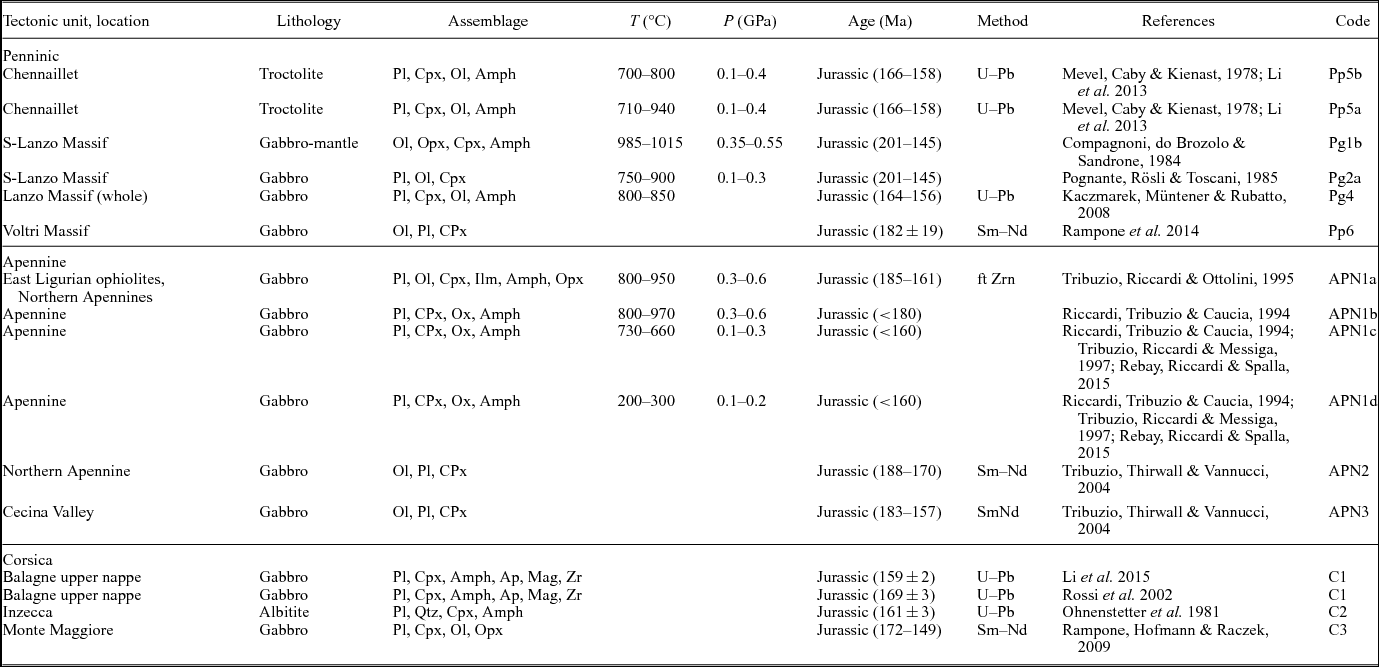
Oceanic mantle rocks coming from the Penninic domain (Table 4) are variably serpentinized peridotites. Based on the relict texture, mineralogy and structural relations with gabbros and rodingites, the serpentinized peridotite of Mt Avic (Table 4) is considered to have an oceanic affinity (Fontana, Panseri & Tartarotti, Reference Fontana, Panseri and Tartarotti2008). Although the gabbroic bodies of the Lanzo Massif are considered to have originated during the opening of the Jurassic–Piedmont Ligurian ocean (Lagabrielle, Fudral & Kienast, Reference Lagabrielle, Fudral and Kienast1989; Pognante, Rösli & Toscani, Reference Pognante, Rösli and Toscani1985) or during the earliest stages of the formation of the embryonic oceanic crust (Kaczmarek, Müntener & Rubatto, Reference Kaczmarek, Müntener and Rubatto2008), the associated peridotites show a more complex affinity as already discussed. The Mg-rich gabbroic rocks of Erro-Tobbio complex in Voltri Massif (Ligurian Alps) is considered as representative of syn-rift melt intrusions in thinned lithospheric mantle exhumed at ocean–continent transition domains (Rampone et al. Reference Rampone, Borghini, Romairone, Abouchami, Class and Goldstein2014). They represent the oldest gabbroic bodies of the Alpine Tethys (201–163 Ma, Rampone et al. Reference Rampone, Borghini, Romairone, Abouchami, Class and Goldstein2014). Because rocks from the Alps are widely deformed and metamorphosed during Alpine subduction and collision, we add ophiolites from the Northern Apennines that escaped pervasive subduction-related metamorphic re-equilibration and the unique case of mafic granulite from the continental crust to the collection of natural data (Tables 3–5). The Northern Apennines are characterized by oceanic and continental units (Fig. 1). Oceanic units are divided into two different groups of thrust nappes – the Internal and External Ligurian units (e.g. Marroni & Pandolfi, Reference Marroni and Pandolfi2007) – strongly deformed under low-grade metamorphic conditions (Marroni & Pandolfi, Reference Marroni and Pandolfi2007; Donatio, Marroni & Rocchi, Reference Donatio, Marroni and Rocchi2013). An ophiolitic sequence of Jurassic age and a sedimentary cover ranging in age from Late Jurassic to Paleocene characterize the Internal Ligurian units (Marroni & Pandolfi, Reference Marroni and Pandolfi2007). In the External Ligurian units, Late Cretaceous sedimentary melanges containing slide-blocks of ophiolites occur at the base of the Upper Cretaceous carbonate turbidites (Helminthoid Flysch; Marroni & Pandolfi, Reference Marroni and Pandolfi2007). The Ligurian units were thrust onto the Tuscan nappes during the Oligo-Miocene post-collisional convergence. The successions of the Tuscan units belong to the Adria passive continental margin, recording in sequence rifting-, cooling- and subsidence-related imprints during the opening of the Liguria–Piemonte Ocean (Marroni & Pandolfi, Reference Marroni and Pandolfi2007). Underlying Tertiary metamorphic units are exposed in rare tectonic windows (Fig. 1).
Granulitic gabbros of the External Liguride Unit associated with felsic granulites locally intrude mantle peridotites (Marroni & Tribuzio, Reference Marroni and Tribuzio1996; Marroni et al. Reference Marroni, Molli, Montanini and Tribuzio1998). The emplacement of the gabbroic protoliths occurs at deep crustal levels of late Carboniferous – early Permian age (approximately 290 Ma), and their country rocks are felsic granulites of the lower continental crust. Most likely in association with the subcontinental mantle, mafic and felsic granulites underwent a multistage exhumation beginning during Permian–Triassic time and ending during Late Triassic – Middle Jurassic time, when they were finally exhumed to shallow levels by extensive brittle faulting (Marroni et al. Reference Marroni, Molli, Montanini and Tribuzio1998). The External Liguride Unit is interpreted as an ocean–continent transition zone (Marroni et al. Reference Marroni, Molli, Montanini and Tribuzio1998).
Some Jurassic oceanic gabbros have been detected in the Apennines (Table 5; Riccardi, Tribuzio & Caucia, Reference Riccardi, Tribuzio and Caucia1994; Tribuzio, Riccardi & Ottolini, Reference Tribuzio, Riccardi and Ottolini1995; Tribuzio, Riccardi & Messiga, Reference Tribuzio, Riccardi and Messiga1997; Rebay, Riccardi & Spalla, Reference Rebay, Riccardi and Spalla2015). The oldest gabbro bodies (169–179 Ma) belong to the External Liguride Unit in the Northern Apennines. Despite their N-MORB affinity, Tribuzio, Thirwall & Vannucci (Reference Tribuzio, Thirwall and Vannucci2004) interpreted these gabbros as having developed during an intermediate stage of the rifting process that led to the opening of the Ligurian Tethys and not strictly related to the oceanic spreading.
The peridotite of the External Liguride Unit has been interpreted as the mantle of an ocean–continent transition zone (Marroni et al. Reference Marroni, Molli, Montanini and Tribuzio1998), while the serpentinized peridotite of the Internal Liguride Unit is suggested to be representative of the Jurassic oceanic lithosphere of the Liguria–Piemonte Ocean (Marroni & Pandolfi Reference Marroni and Pandolfi2007; Donatio, Marroni & Rocchi, Reference Donatio, Marroni and Rocchi2013).
5. Comparison between the model predictions and the natural data
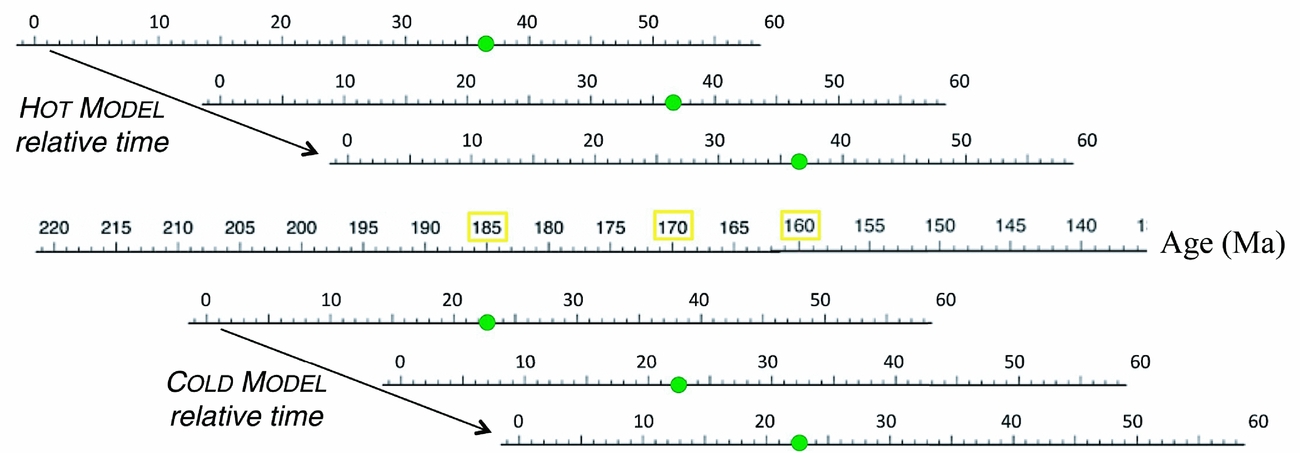
Before proceeding with the comparison between the model predictions and the natural data, it is necessary to reference the relative time of the numerical simulation with respect to the natural ages. To achieve this goal, we decided to match the beginning of the mantle partial melting in the model with the ages of the gabbros available in the literature (Table 5). In particular, we chose the three absolute ages of 160 Ma, 170 Ma and 185 Ma interpreted by different authors (Tribuzio, Riccardi & Ottolini, Reference Tribuzio, Riccardi and Ottolini1995; Tribuzio, Thirwall & Vannucci, Reference Tribuzio, Thirwall and Vannucci2004; Li et al. Reference Li, Faure, Lin and Manatschal2013, Reference Li, Faure, Rossi, Lin and Lahondère2015) as the oldest gabbro ages of Liguria–Piemonte Ocean; they can therefore be considered the temporal markers of the early oceanic spreading. Figure 8 depicts the time referencing of both models with respect to the three chosen absolute ages.
Time references from the hot and cold models with respect to the age of the oldest gabbros (160 Ma, 170 Ma and 185 Ma), based on the literature for the Northern Apennines and Western Alps (Tribuzio, Riccardi & Ottolini, Reference Tribuzio, Riccardi and Ottolini1995; Li et al. Reference Li, Faure, Lin and Manatschal2013; Rampone et al. Reference Rampone, Borghini, Romairone, Abouchami, Class and Goldstein2014). Green circles identify the times when the mantle partial melting occurs in the hot model (36.4 Ma) and in the cold model (22.4 Ma).
The data from the continental crust (Tables 2, 3) are compared with the continental markers; the data from the mantle (Table 4) are compared with the dry or serpentinized mantle according to the estimated P–T conditions and rock assemblages. In the following, the process starting from the exhumation of serpentinized mantle and proceeding through the oceanic spreading is referred to as ‘oceanization’. The oceanic spreading leading to the formation of the Liguria–Piemonte Ocean starts when the conditions favourable for mantle partial melting are attained in the system. We compare the pressure–temperature values predicted for markers belonging to the oceanic lithosphere with the P–T estimates available for gabbros belonging to Alpine and Apennine ophiolitic complexes (Table 5), as well as those available for the oceanic mantle (Table 4).
To verify if the simulated geodynamic context can reproduce a thermal state that is compatible with that recorded by the lithosphere during the Permian–Triassic period, in Figure 9 we show the duration of the agreement between the predictions and the natural data for the three different absolute ophiolite ages in terms of lithology and coincident P–T values compared to the radiometric (black thick segments) and geologic (grey thick segments) ages of the natural data. In the following discussion, we refer to a ‘complete fit’ when there is agreement between the model predictions and the natural data in the lithology, P–T values and ages. The fit is considered ‘partial’ if age coincidence is lacking. The comparative analysis takes into account the natural data with their error margins (Tables 2–5).
Duration of the agreement between the predictions and the natural data as well as number of fitting markers (colours) for the three different ages of the oldest gabbros (160 Ma, 170 Ma and 185 Ma, dashed black lines) in terms of lithological affinity and coincident P–T values compared to the radiometric (black thick segments) and geologic (grey thick segments) ages of the natural data. In the text, we refer to the result as a ‘complete fit’ when the model predictions and the natural data of the lithological affinity, P–T values and ages agree. The fit is considered ‘partial’ if age agreement is lacking. Panel (a) refers to the hot model, whereas panel (b) refers to the cold model. The light grey area represents the duration of the numerical simulation. The codes are defined in Tables 2–5.

The predictions of both the hot and cold models show complete fits with the same data, although the number of fitting markers is in general lower in the cold model than in the hot model. Complete fits are realized with a maximum of 13 data points out of the available 44: 10 are of the oceanic lithosphere type (Pp5a, Pp5b, Pp6, Pg1b and Pg2a, Penninic domain; and APN1a, APN1b, APN1c, APN1d and APN3, Apennine domain), and 2 are of the pre-oceanic lithosphere type (Ap5a, Pg3b and Pg3c, Austroalpine domain). Good agreement is obtained for all of the oceanic lithosphere type markers with the natural data from the Alpine and Apennine ophiolites for all of the ages proposed in the literature.
The predictions do not show a complete fit with the continental crust data. Nevertheless, the hot model reproduces thermo-barometric conditions that are compatible with those of most of the continental crust data in the interval during 220–150 Ma, according to the time of the oldest ophiolitic ages. A similar situation holds for the cold model, although with a very low number of markers. However, the radiometric ages of these data are older than the oldest model predictions.
Some data, that is, Sp1 (Eisacktal), Sp3 (Dervio-Olgiasca) and Sp5a and Sp5b (Ivrea) which are from the Southalpine domain, Ap17 (Sopron) and Ap7 and Ap8 (Valpelline) which are from the Austroalpine domain and Pp4 (Gruf) which is from the Penninic domain, do not show any agreement, even thermo-barometric, because the estimated temperatures are higher than the predicted temperatures.
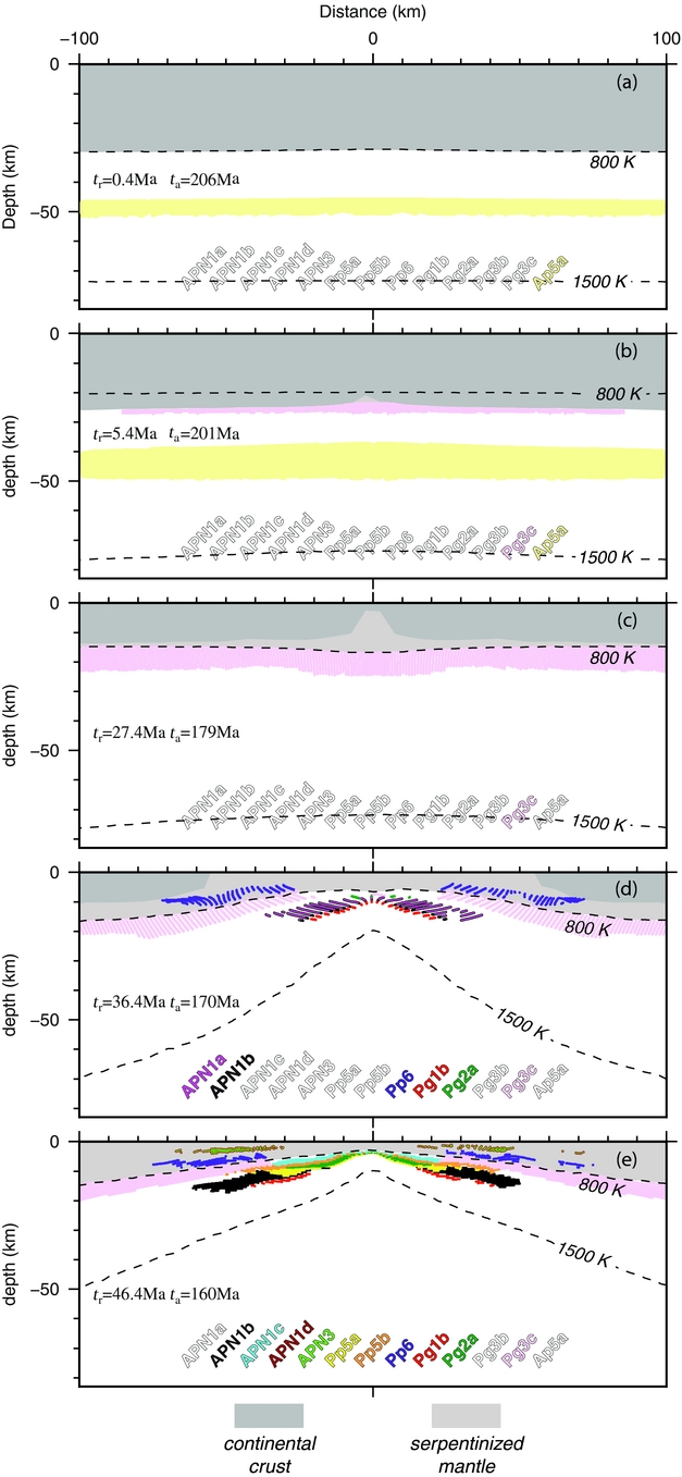
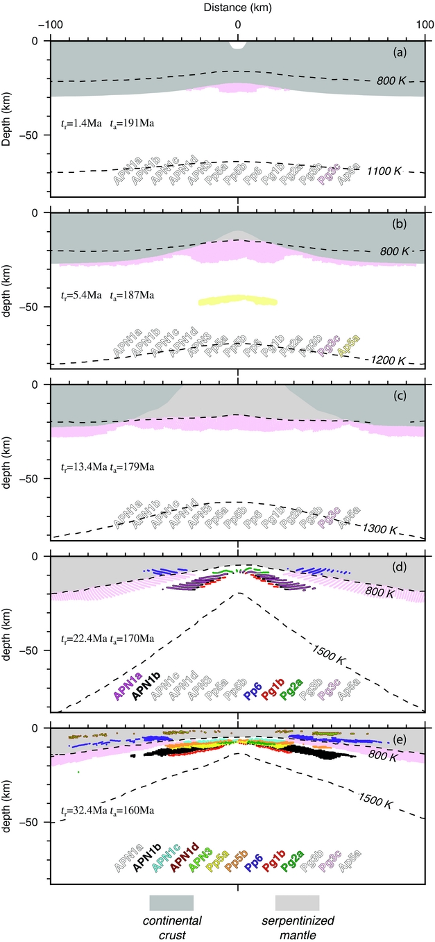
Figures 10 and 11 depict the spatial distributions of the markers that exhibit complete fits with the data for the hot and the cold models, respectively. With the exception of the Pg3c and Ap5a (continental mantle, Austroalpine domain) data, the P–T conditions that are compatible with those of the other natural data are predicted only in a 200 km wide region centred at the ridge and only after the formation of the oceanic lithosphere (Figs 10d, e, 11d, e). The Pg3c datum fits the mantle-type markers at shallow structural levels only after a significant thermo-mechanical thinning of the lithosphere. This occurs after approximately 5.4 Ma in the hot model, affecting a large amount of the continental lithospheric mantle (Fig. 10b). In the cold model, the fitting starts very early and affects only a 60 km wide area around the future ridge, concurrently with the thermal thinning localization. For both models, the fitting persists until the late stages of the evolution and affects the shallow structural levels of the entire non-serpentinized lithosphere. The hot model predicts P–T conditions that are compatible with the Ap5a datum (continental mantle, Austroalpine domain) starting at the beginning of the simulation (Fig. 10a), while in the cold model the favourable conditions occur only after significant heating of the system (Fig. 11b). This result supports the idea that Ap5a is a representative slice of the continental mantle under the perturbed P–T conditions rather than under the thermal regime of a stable lithosphere. Pg1b and Pg2a, both of which belong to the gabbroic rocks of the Lanzo Massif for both the hot and cold models, exhibit a complete fit with markers of the oceanic lithosphere type but at different structural levels. Pg1b agrees at deeper structural levels (Figs 10d, 11d), consistent with a gabbroic melt impregnation of the lithosphere (Compagnoni, di Brozolo & Sandrone, Reference Compagnoni, di Brozolo and Sandrone1984). Instead, Pg2a agrees at shallower levels (Figs 10d, 11d), in agreement with a decompression stage of an older subcontinental lithospheric mantle under hydrated conditions (Pognante, Rösli & Toscani, Reference Pognante, Rösli and Toscani1985). Fits with Pp6 (Mont Avic serpentinized peridotite), APN1a (gabbros of North Apennines ophiolites) and APN1b (gabbros of Apennines Ophiolites) data start at the beginning of the oceanization (Figs 10d, 11d) and can be compatible with either the oceanic lithosphere or the ocean–continent transition zone. During oceanic spreading, the complete fit localizes at the marginal portions of the oceanic basin (Figs 10d, e, 11d, e). Finally, the complete fit with the APN1c, APN1d and APN3 (gabbros and mantle of Apennines ophiolites) and Pp5a and Pp5b (Chenaillet) data occurs during oceanic spreading and at the appropriate litho-structural levels of the oceanic lithosphere (Figs 10e, 11e).
Spatial distribution of the markers that guarantee a complete fit of the data for the hot model at different stages of the evolution. The dashed black lines indicate the 800 K and 1500 K isotherms. The colours identify the markers showing a complete fit with the natural data as specified in the legend; t r indicates the time span from the beginning of the simulation and t a indicates the absolute age constrained choosing the oldest gabbro age at 170 Ma (see discussion in the text). The codes are defined in Tables 2–5.
Spatial distribution of the markers that guarantee a complete fit of the data for the cold model at different stages of the evolution. The dashed black lines indicate the 800 K and 1500 K isotherms. The colours identify the markers showing a complete fit with the natural data specified in the legend; t r indicates the time span from the beginning of the simulation and t a indicates the absolute age constrained choosing the oldest gabbro age at 170 Ma (see discussion in the text). The codes are defined in Tables 2–5.
6. Discussion
The model of crustal extension presented here, characterized by a weak lower crust and mantle serpentinization, results in symmetric rifting of the continental lithosphere and exhumation of a serpentinized lithospheric mantle. Our results support the idea that the occurrence of serpentinization of the mantle can favour the exhumation of the lithospheric mantle before the oceanic spreading in agreement with Lagabrielle & Cannat (Reference Lagabrielle and Cannat1990) and Pérez-Gussinyé et al. (Reference Pérez-Gussinyé, Morgan, Reston and Ranero2006).
The onset of lithospheric thinning localized around the future ridge strongly depends on the initial lithosphere thermal state: for a cold and strong lithosphere, the thinning is very rapid (after approximately 4.4 Ma) with respect to a hot and weak lithosphere (after approximately 15.4 Ma). Similarly, the time span between the onset of thinning and the occurrence of crustal break-up is shorter for a cold lithosphere (approximately 3 Ma) than for a hot lithosphere (approximately 16 Ma). These dynamics are attributable to the concurrent roles of the prescribed far-field traction and mantle upwelling flow. In the hot model, the contribution of the upwelling mantle flow to the lithosphere extension becomes efficient only in the advanced stages of the evolution, after the onset of the mantle partial melting. In contrast, for the cold model, both forces concur to the extension dynamics from the early stages of the evolution. These results agree with the models by Brune & Autin (Reference Brune and Autin2013) and Manatschal, Lavier & Chenin (Reference Manatschal, Lavier and Chenin2015) in which the break-up of a hotter and weaker lithosphere occurs later than in a colder and stronger lithosphere. In the case of a higher thermal state of the pre-rifting lithosphere, the viscous crustal layer is thicker than the brittle portion; consequently, the brittle strain softening is less efficient at focusing the deformation into discrete shear zones (Brune & Autin, Reference Brune and Autin2013). Lavier & Manatschal (Reference Lavier and Manatschal2006) and van Avendonk et al. (Reference Van Avendonk, Lavier, Shillington and Manatschal2009) suggest the opposite behaviour when the strong gabbroic lower crust is taken into account. In their models, a cold and strong lithosphere results in a longer rifting duration. On the other hand, the occurrence of a strong lower crust for the Alpine pre-rifting lithosphere is in contrast to the lithostratigraphy of the pre-Alpine continental crust. Given the number and size of Permian–Triassic gabbroic intrusions in the Alpine crust, the amount of detectable gabbroic rocks is less than 5 % of the total pre-Alpine lower continental crust actually exposed along the whole Alpine belt, which can be estimated from the tectonic map of the Alps (Bigi et al. Reference Bigi, Castellarin, Coli, Dal Piaz, Sartori, Scandone and Vai1990; Schmid et al. Reference Schmid, Fügenschuh, Kissling and Schuster2004) taking into account both units deeply involved in or escaping the Alpine subduction. Even considering a lower crust of the pristine passive margin that is richer in gabbroic rocks, it is reasonable to predict that, during the Alpine convergence, a selective tectonic sampling of the gabbro-poor lower crust does not occur. A coherent gabbroic lower crust for the Alpine pre-rifting lithosphere therefore seems unlikely.
For both chosen initial thermal configurations of the lithosphere, the exhumation of the serpentinized mantle starts before the oceanic spreading and the mantle partial melting (considered in our study coincident with gabbros formation), making the model compatible with the magma-poor rifting suggested for the Alpine case (e.g. Lavier & Manatschal, Reference Lavier and Manatschal2006; Pérez-Gussinyé et al. Reference Pérez-Gussinyé, Morgan, Reston and Ranero2006; Manatschal & Müntener, Reference Manatschal and Müntener2009; Manatschal, Lavier & Chenin Reference Manatschal, Lavier and Chenin2015), developing an ocean–continent transition zone similar to Galizia margin (e.g. Boillot, Girardeau & Kornprobst, Reference Boillot, Girardeau and Kornprobst1989; Manatschal, Reference Manatschal2004; Hébert et al. Reference Hébert, Beaudoin, Rochon and Gardien2008). The exhumation of a serpentinized lithospheric mantle before the oceanic spreading of the Liguria–Piemonte Ocean is also suggested based on the geochemical analysis of the syn-rift Alpine crust and sediments (Pinto et al. Reference Pinto, Manatschal, Karpoff and Viana2015).
For both the hot and cold models, the mantle partial melting does not appear immediately after the crustal break-up but after approximately 5 Ma in the hot model and after approximately 15 Ma in the cold model. This result is dependent on the thermal field predicted when the crustal break-up occurs. The hot model predicts more suitable thermo-barometric conditions for mantle melting a few million years after the crustal break-up. In contrast, in the cold model a long time is required to increase the thermal state to satisfy the pressure–temperature conditions that are suitable for mantle melting. Despite the different partial timings of each stage in the two models, once the serpentinization starts and the deformation localizes around the future ridge, the time required for the mantle partial melting and the beginning of oceanic spreading is comparable in the two models: 18 Ma for the cold model and 21 Ma for the hot model.
The continental crust thickness sensibly decreases during the extension but with different rates. In the hot model, the crustal thickness decreases from 30 km to approximately 18 km at the margin and to approximately 5 km close to the OCTZ within 31.4 Ma after the beginning of the evolution. In the cold model, it decreases from 30 km to approximately 22 km at the margin and to approximately 20 km close to the OCTZ within 21.4 Ma after the beginning of the evolution. Afterwards, in both models no further significant thinning occurs within the continental crust. The hyperextended margin envisaged by the hot model satisfies the model of an Alpine Tethys hyperextended system (Manatschal, Lavier & Chenin, Reference Manatschal, Lavier and Chenin2015). Our results indicate that in the proximity of the ridge, for both models, the extension rate at the base of the crust increases by a factor of 2–4 from the continental break-up to oceanization, in agreement with Whitmarsh, Manatschal & Minshull (Reference Whitmarsh, Manatschal and Minshull2001). Furthermore, at the advanced stages of the extension after the beginning of oceanic spreading, the extension rate may overcome the far-field traction.
A thinned continental crust (passive margin), an ocean–continent transition zone and an oceanic lithosphere characterize the final structure of the system from the periphery to the centre of the model domain for both thermal states. Our results show that the formation of the OCTZ starts 5–15 Ma before the partial melting of the mantle and develops with a size ranging over 160–280 km (according to the initial thermal configuration of the lithosphere), which is compatible with the observations of Galicia Margin (e.g. Boillot, Beslier & Girardeau, Reference Boillot, Beslier, Girardeau, Banda, Torné and Talwani1995; Hébert et al. Reference Hébert, Beaudoin, Rochon and Gardien2008) and similar to the interpretation for the Alpine rift (Manatschal & Müntener, Reference Manatschal and Müntener2009). This suggests that if the estimate of the oceanic basin width is based simply on the coincidence between the continental crust break-up and the onset of gabbros emplacement, as stated in several models proposed for the Alpine domain (e.g. Li et al. Reference Li, Faure, Lin and Manatschal2013), the effective basin width will be underestimated. In particular, Li et al. (Reference Li, Faure, Lin and Manatschal2013) estimated a basin width of 300 km after 10 Ma of extension at a full spreading rate of 3 cm a−1. In contrast, our model indicates that the extension of the basin would range over 360–480 km after the same time of 10 Ma for a full extension rate of 2.5 cm a−1.
The comparison between the natural data and the model predictions shows good agreement with all of the oceanic data for both the hot and cold models. In contrast, the comparison with the data from the continental crust lacks a complete fit because ages are not coincident. The lithological and thermal fits predicted by the hot and cold models with significant delays (from the Permian–Triassic to the Late Triassic – Late Jurassic periods; Figs 7, 9) suggest that, according to both models, the effects of a positive thermal anomaly should be recorded in the continental crust of both passive margins at 220–150 Ma. These effects have not yet been detected in the pre-Alpine continental crust of the Alps and Apennines. Similarly, the mantle partial melting occurs in both models 36.4 Ma and 22.4 Ma after the beginning of the extension in the hot and cold models, respectively, that would correspond to the early gabbros at 185 Ma, which is significantly younger than the Permian–Triassic continental gabbro emplacements. This time misfit supports the interpretation predicting a thermo-mechanical perturbation of the continental lithosphere in this portion of the Tethys due to the Variscan collision and the late orogenic extension (Spalla et al. Reference Spalla, Zanoni, Marotta, Rebay, Roda, Zucali, Gosso, Schulmann, Martínez Catalán, Lardeaux, Janoušek and Oggiano2014). In addition, the more favourable thermal regime predicted by the hot model could be due to a previously perturbed system either by the Variscan orogenic collapse or by an already thermally eroded and softened lithosphere. However, the sole orogenic collapse mechanism is not sufficient to reproduce the thermo-barometric conditions of the HT-LP Permian–Triassic metamorphism and intense igneous activity recorded in the continental lithosphere (Marotta & Spalla, Reference Marotta and Spalla2007; Marotta, Spalla & Gosso, Reference Marotta, Spalla, Gosso, Ring and Wernicke2009).
Finally, although the symmetry of the predicted thermal anomaly around the future ridge, HT natural parageneses from the Permian–Triassic continental lithosphere of the Alps are concentrated in the Austroalpine and Southalpine domains, while they are totally lacking in the Helvetic domain. This distribution of HT-LP metamorphic assemblages supports the interpretation of an asymmetric rifting (e.g. Lardeaux & Spalla, Reference Lardeaux and Spalla1991; Marotta, Spalla & Gosso, Reference Marotta, Spalla, Gosso, Ring and Wernicke2009).
7. Conclusions
We developed a 2D thermo-mechanical numerical model of passive rifting to investigate the evolution of the lithosphere of the Alps and the Northern Apennines during the transition from continental rifting to oceanic spreading of the Alpine Tethys. The model accounts for the crustal extension of a weak lower crust and mantle serpentinization, and results in symmetric rifting and denudation of the serpentinized lithospheric mantle.
A thinned continental crust (passive margin), an ocean–continent transition zone and an oceanic lithosphere characterize the final structure of the system. The thickness of the passive margin decreases over time from 30 km to 18 km (hot model) or 22 km (cold model) at the model boundaries and to 5 km (hot model, hyperextended margin configuration) or 20 km (cold model) close to the ocean–continent transition zone.
The mantle serpentinization starts before the crustal break-up, and the denudation occurs before the oceanic spreading. In addition, a hot and weak lithosphere evolves to oceanization slower than a cold and strong lithosphere, with a comparable time interval after the onset of serpentinization.
Our results indicate that, if the estimated basin width is based simply on the coincidence between the continental crust break-up and the onset of the gabbros emplacement, the effective width of the basin domain will be underestimated. The mantle denudation starts several million years before partial melting, generating an ocean–continent transition zone from the passive continental margin to the oceanic lithosphere with a size ranging over 160–280 km in a magma-poor rift pre-Alpine configuration.
The thermo-barometric predictions with their modelled timing were compared with the natural data derived from continental and oceanic rocks from the Alps and Apennines of Permian–Jurassic age, and the predictions from the hot model, which also promotes the development of hyperextended Alpine margins, agree with natural data better.
Our results support the idea that the Tethyan rifting should begin in a perturbed continental lithosphere, likely ascribable to the previous Variscan subduction-collision, as widely supported by the occurrence of HP metamorphic relics in the different Alpine structural domains. In fact, if rifting developed in a stable lithosphere, Triassic–Jurassic HT-LP metamorphism is predicted together with gabbro-basalt production younger than 185 Ma instead of the observed Permian–Triassic metamorphic and igneous records. Indeed, this has never been detected in the Alpine continental crust.
In addition, the distributions of the Permian–Triassic continental gabbros and the high-temperature metamorphism in the Austroalpine and Southalpine domains support the idea that it was asymmetric rifting in which the lithospheric signature of the Variscan subduction-collision can be a constraining inheritance for the successive geometry.
These ideas could be further confirmed by a new model that accounts for the previous history and the thermo-rheological consequences of Variscan Orogeny as initial configuration (as in Marotta, Spalla & Gosso, Reference Marotta, Spalla, Gosso, Ring and Wernicke2009) and evolves though continental break-up and the successive oceanization as in the present study.
Acknowledgements
The research was supported by PRIN 2011 (2010AZR98L) (Birth and death of oceanic basins: geodynamic processes from rifting to continental collision in Mediterranean and circum-Mediterranean orogens). The authors thank T. Gerya and U. Ring for fruitful suggestions. We also thank the editor and the two anonymous reviewers for their thorough review. All figures were created using GMT plotting software (Wessel & Smith, Reference Wessel and Smith2001) and Adobe Illustrator®.



