


1. Introduction
Sediments and glaciers are inextricably linked. Glaciers produce sediment through abrasion and plucking and override sediments during glacier advance. Consequently, it is common for glaciers to be partially or mostly soft-bedded (Benn and Evans, Reference Benn and Evans2010; Cuffey and Paterson, Reference Cuffey and Paterson2010). Glaciers interact with these sediments to create complex and variable landforms, such as drumlins, eskers, lateral and end moraines, kame terraces, outwash deposits and till plains, many of which are ubiquitous in glacial landscapes (Menzies and others, Reference Menzies, van der Meer and Shilts2017). The history of these glacial deposits can be inferred from sedimentary structures, but observing geomorphic processes in an active glacial setting is the best way to study glacial landform construction. Taku Glacier, a tidewater glacier in Southeast Alaska that was advancing as recently as 2015 CE, provides such an opportunity.
Understanding glacier landform construction is not only important for reconstructing past glacial environments, but also for predicting future glacier evolution (especially for tidewater glaciers) and associated changes in sea level. The stability of tidewater glaciers is thought to be strongly influenced by the deposition and re-working of their end moraines (Post and others, Reference Post, O'Neel, Motyka and Streveler2011; Brinkerhoff and others, Reference Brinkerhoff, Truffer and Aschwanden2017), which act to both protect the glaciers from the ocean and to provide additional flow resistance that enables the upper reaches of the glaciers to thicken (Fischer and Powell, Reference Fischer and Powell1998; Amundson, Reference Amundson2016).
The physical processes by which sediment is transported towards the termini of tidewater glaciers are not completely understood due to limited observations. The current understanding is that subglacial sediment transport can occur via glaciofluvial activity (Walder and Fowler, Reference Walder and Fowler1994; Swift and others, Reference Swift, Nienow and Hoey2005; Motyka and others, Reference Motyka, Truffer, Kuriger and Bucki2006), basal freeze-on, sediment deformation or glaciotectonism (Alley and others, Reference Alley1997; Smith and others, Reference Smith2007). Thrust-block moraines (also known as composite ridges) can form in proglacial sediments when the horizontal component of the weight of glacial ice on a cohesive ice-marginal sediment wedge overcomes the friction at the base of the wedge, resulting in thrust faulting (Motyka and Echelmeyer, Reference Motyka and Echelmeyer2003; Kuriger, Reference Kuriger2005; Kuriger and others, Reference Kuriger, Truffer, Motyka and Bucki2006); Taku Glacier has produced thrust-block moraines in the past. Push moraines (ridges of loose sediments formed when pushed by the advancing ice front) also form at Taku Glacier, but are of relatively small extent (Kuriger and others, Reference Kuriger, Truffer, Motyka and Bucki2006). At Taku Glacier, glaciofluvial removal of soft marine sediments is thought to be the main sedimentary process near the glacier terminus due to the high excavation rates observed there. These high sediment removal rates, which locally exceed 1 m a−1 (Motyka and others, Reference Motyka, Truffer, Kuriger and Bucki2006), are difficult to reconcile with other, slower processes (Hallet and others, Reference Hallet, Hunter and Bogen1996; Alley and others, Reference Alley1997). When these sediments emerge from the subglacial environment, they may form proglacial outwash fans, which can experience deposition rates of centimeters per year (Korsgaard and others, Reference Korsgaard2015).
Glaciofluvial sediment removal rates depend on a variety of constantly changing factors, including substrate properties, patterns of water inputs, and the state of the subglacial drainage system (Swift and others, Reference Swift, Nienow and Hoey2005). Fluctuations in the subglacial water system occur on daily to seasonal timescales (Swift and others, Reference Swift, Nienow and Hoey2005; Perolo and others, Reference Perolo, Bakker, Gabbud, Moradi, Rennie and Lane2019; Vore and others, Reference Vore, Bartholomaus, Winberry, Walter and Amundson2019) due to the progressive formation of englacial and subglacial conduits and changes in water availability. Sediment evacuation efficiency (the relationship between sediment load and water discharge) can change, sometimes abruptly, over the melt season or during diurnal or storm cycles (Hodson and Ferguson, Reference Hodson and Ferguson1999; Riihimaki and others, Reference Riihimaki, MacGregor, Anderson, Anderson and Loso2005; Singh and others, Reference Singh, Haritashya, Ramasastri and Kumar2005; Swift and others, Reference Swift, Nienow and Hoey2005). Early in the melt season, the subglacial drainage system is inefficient and experiences high water pressures, enough to lift glacier ice and allow water to come into contact with large volumes of basal sediment (Hooke and others, Reference Hooke, Wold and Hagen1985; Delaney and others, Reference Delaney, Werder and Farinotti2019). In this setting, water inputs from melting or rain events can then cause subglacial water to flow fast enough to evacuate sediments (Swift and others, Reference Swift, Nienow and Hoey2005). Sediment mobilization eventually declines as frictional heating from water flow widens subglacial ice channels and they coalesce into an efficient, lower-pressure drainage system (Röthlisberger, Reference Röthlisberger1972; Shreve, Reference Shreve1972). Later in the melt season, sediment evacuation rates are able to rise again once strong diurnal water pressure cycles appear (Swift and others, Reference Swift, Nienow and Hoey2005). However, though water discharge reaches its annual peak at this time, sediment removal efficiency decreases due to inconsistencies and spatially limited contact between flowing water and subglacial materials (Hooke and others, Reference Hooke, Wold and Hagen1985). Taku Glacier experiences seasonal changes in its hydrological system well evidenced by a ‘spring speed-up’ every April and May (Truffer and others, Reference Truffer, Motyka, Hekkers, Howat and King2009), so we expect to see seasonal changes in its sediment removal efficiency in any analysis of its sediment regime over time.
Our goal is to improve our understanding of sediment evacuation, transport and deposition, and their implications for the future evolution of the glacier bed and foreland and resulting consequences for tidewater glacier stability. To achieve this goal, we conducted a comprehensive study at Taku Glacier from 2014 to 2016, which included repeat radio echo sounding (RES) measurements, analysis of digital elevation models and time-lapse photography, in order to map current sediment removal and deposition patterns and to document ongoing landform creation and destruction. In this paper, we focus on observations of sediment reworking (i) in the near-terminus subglacial environment, (ii) on an active proglacial outwash fan, (iii) along a thrust block moraine complex at the terminus and (iv) in the subglacial environment 2–4 km further upstream. We find that these four locations experience interrelated and ongoing landscape modification processes.
2. Study area
Taku Glacier has a long history of research and a compelling reason to be studied: it has, until recently (2015 CE) been the only advancing glacier in the Juneau Ice Field region. It is also an important glacier in local native history. The indigenous Tlingit occupied this region for centuries and their name for Taku is T'aakú Kwáan Sít'i (T'aakú People's Glacier). The word ‘T'aakú’ translates to ‘Flood of Geese’ (Southeast Native Subsistence Commission Place Name Project, 1994–2001). Numerous publications describe the background and character of this glacier (e.g., Lawrence, Reference Lawrence1950; Motyka and Post, Reference Motyka and Post1995; Nolan and others, Reference Nolan, Motyka, Echelmeyer and Trabant1995; Post and Motyka, Reference Post and Motyka1995; Motyka and Beget, Reference Motyka and Beget1996; Motyka and Echelmeyer, Reference Motyka and Echelmeyer2003; Motyka and others, Reference Motyka, Truffer, Kuriger and Bucki2006; Kuriger and others, Reference Kuriger, Truffer, Motyka and Bucki2006; Truffer and others, Reference Truffer, Motyka, Hekkers, Howat and King2009; Pelto and others, Reference Pelto, Kavanaugh and McNeil2013), which we here summarize.
Taku Glacier (Fig. 1) as of 2020 CE covers an area of 725 km2 (McNeil and Baker, Reference McNeil and Baker2019) and has a length of 55 km (Nolan and others, Reference Nolan, Motyka, Echelmeyer and Trabant1995; McNeil and Baker, Reference McNeil and Baker2019). The local maritime climate results in large snow accumulation rates at the head of the glacier (~3 m w.e. a−1) and high seasonal ablation rates at the terminus (13–15 m w.e. a−1) (Truffer and others, Reference Truffer, Motyka, Hekkers, Howat and King2009; McNeil, Reference McNeil2016).
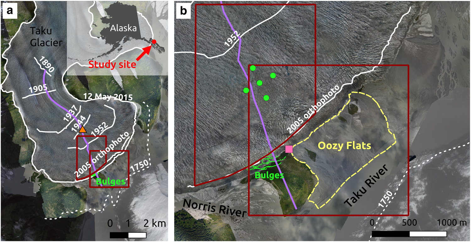
Overview of the study area, showing past terminus positions (white), locations of close-up figures (left red box, Fig. 6, right red box, Fig. 8), borehole locations (green dots), 2015 GPS station location (orange triangle), bulge locations from a 2001 GPS survey (green lines), dye sampler location (pink square), and the location of the profile cross section in Fig. 4 (purple line). The imagery mosaic was produced using a camera mounted on a Cessna 180, which flew a grid over the lower Taku Glacier in August of 2015 (Larsen, Reference Larsen2018). The images were orthorectified using the methods of Nolan and others (Reference Nolan, Larsen and Sturm2015). Gaps in coverage are filled in using imagery from Google Earth (2010).
Like other tidewater glaciers, Taku Glacier undergoes cycles of slow advance and rapid retreat (Post and others, Reference Post, O'Neel, Motyka and Streveler2011). The glacier has cycled through 5 advance/retreat phases over the last 3000 years, often out of phase with climate fluctuations (Post and Motyka, Reference Post and Motyka1995; Motyka and Beget, Reference Motyka and Beget1996). Sediment mass balance drives the glacier advance and retreat cycles with climate as a modulator (Alley, Reference Alley1991; Post and others, Reference Post, O'Neel, Motyka and Streveler2011; Brinkerhoff and others, Reference Brinkerhoff, Truffer and Aschwanden2017). The glacier has been advancing since at least 1890 CE, overriding and eroding subglacial sediments that are then re-deposited at its terminus. These sediments have now separated the glacier from ocean water, preventing subaqueous melt and calving (Nolan and others, Reference Nolan, Motyka, Echelmeyer and Trabant1995; Post and Motyka, Reference Post and Motyka1995).
In 1750 CE, the glacier terminus was at its Little Ice Age maximum (Lawrence, Reference Lawrence1950) and stretched across the Taku River (Fig. 1a), damming it and creating a 70 km long lake (Post and Motyka, Reference Post and Motyka1995). Eventually, the river breached the glacier terminus, resulting in catastrophic lake drainage, the formation of deep channels in downstream sediments, and initiation of glacier retreat (Post and Motyka, Reference Post and Motyka1995). The retreat resulted in a large proglacial fjord, informally referred to as ‘Taku Fjord’ (Post and Motyka, Reference Post and Motyka1995).
The oral history of the Tlingit people makes special mention of Taku Glacier, which blocked access to the continental interior until this retreat occurred. The earliest written observations of the glacier come from the Vancouver expedition in 1794. The Vancouver expedition had little knowledge of glacier dynamics, but their records implied that Taku Glacier was in a retracted position and had a vertical calving front. On 10 and 11 August 1794, the expedition observed floating ice in Taku Inlet, an open basin long enough to imply that Taku Glacier had retreated ~10 km since 1750, and, coming from the mountain valleys, ‘immense bodies of ice, that reached perpendicularly to the surface of the water in the basin, which admitted of no landing place for boats’ (Vancouver, Reference Vancouver1801).
By the time Taku Glacier was first mapped by the US Coastal and Geodetic Survey (USCGS) in 1890, the glacier terminus was advancing into Taku Fjord, which was at that time 7 km long and 100 m deep. The fjord rapidly filled with sediments from Taku River and Taku Glacier (Motyka and Post, Reference Motyka and Post1995), and by 1931 shoals appeared in front of the terminus (Post and Motyka, Reference Post and Motyka1995). The USCGS resurveyed Taku Fjord between 1937 and 1956, revealing ongoing proglacial accumulation of marine sediments. Push moraines rose above sea level in 1948, and have since been prograding down-fjord along with the advancing terminus. Some of these push moraines appear to have been formed by episodic thrusting, with the most recent event ending in 2001 (Motyka and Echelmeyer, Reference Motyka and Echelmeyer2003; Kuriger, Reference Kuriger2005; Kuriger and others, Reference Kuriger, Truffer, Motyka and Bucki2006). These push moraine studies were the first to measure sediment landform changes at Taku Glacier. Additional geomorphic processes have impacted the glacier ice itself, but have not yet been recorded.
Proglacial shoal formation is an ongoing process that has kept Taku Glacier in the advancing phase of the tidewater glacier cycle. The shoal has, in the recent past, experienced rapid erosion from the nearby Norris River (Fig. 1b), which floods periodically due to subglacial lake drainage events from the adjacent Norris Glacier. Aerial images show that the Norris River carved away > 100 m of the proglacial shoal between August 2004 and September 2005. The Taku River bordering the proglacial shoal to the east also floods periodically due to outburst floods from the Tulsequah Glacier upstream (Neal, Reference Neal2007). Sediment contributions to the shoal from Taku Glacier are currently able to offset fluvial erosion.
In this study, we focus on quantifying sediment excavation and deposition in the near-terminus subglacial and proglacial environments (Fig. 1). We choose these areas because they are rapidly changing and/or have been studied before. These sites, include (i) the ‘lower study area’, a 2 km × 2 km area of the terminus (red rectangle on the left in Fig. 1b) that overlays a subglacial trough that is ~ 250 m wide and 140 m deep (Motyka and others, Reference Motyka, Truffer, Kuriger and Bucki2006); (ii) an outwash plain containing the major outlet streams of the central part of Taku Glacier's piedmont-like terminus (referred to as ‘Oozy Flats’ and outlined in yellow in Fig. 1b); (iii) a series of proglacial thrust moraines, referred to as ‘bulges’, shown as green lines in Fig. 1a (Kuriger and others, Reference Kuriger, Truffer, Motyka and Bucki2006); and (iv) the ‘upper study area’, a 1 km × 3 km area of the glacier bed, located adjacent to the eastern glacier edge and 3 km from the present-day terminus (see black dots in Fig. 2 for RES locations). The upper study area spans the 1905 and 1944 terminus locations (Motyka and others, Reference Motyka, Truffer, Kuriger and Bucki2006). The first three of these areas overlie a thick sediment package, with a minimum thickness that is constrained by the 1890 bathymetric survey.
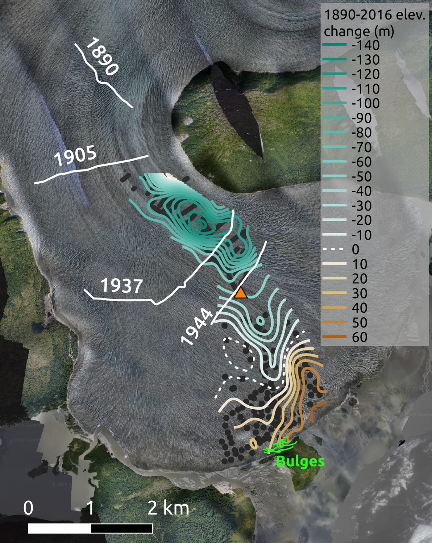
Areas where the current glacier bed (from radar) is above the 1890 fjord floor (brown topo lines) and areas where the glacier has eroded past the 1890 fjord floor (green topo lines). The boundary between the two is marked in white. Black dots show the locations of radar measurements. The proglacial bulges, as surveyed in 2001, are shown in green. The orange triangle shows the location of the 2015 GPS station.
3. Methods
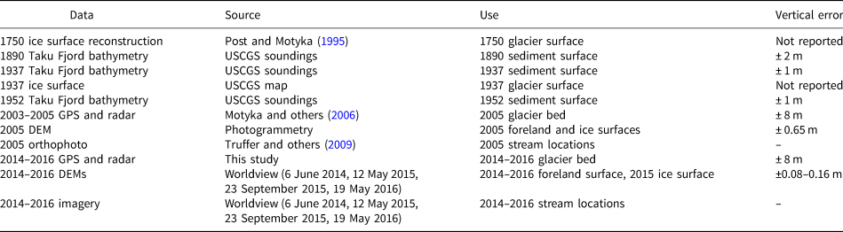
This study relies on multiple datasets: repeat RES surveys to quantify changes in subglacial topography; various digital elevation models (DEMs) to document changes in proglacial topography; time-lapse photography to observe proglacial erosion and deposition; and aerial and satellite imagery to locate the changing positions of outwash streams (Table 1). Additionally, we use glacier bed soundings and GPS ice surface elevations from a 2016 RES survey to calculate the hydraulic potential at the glacier bed, and dye tracing to study the glacier's hydrological system. We also estimate the elevation of the bedrock surface beneath the glacier ice and subglacial sediments by fitting parabolas to DEMs of the glacial valley walls. In combination, these data sets allow us to investigate what excavation/deposition mechanisms are in play, how water is routed, what effect it has on the sediment surface, how much sediment is available for Taku Glacier to remove, and what we can expect about future landform evolution.
Data used in this study
3.1 Sediment thickness
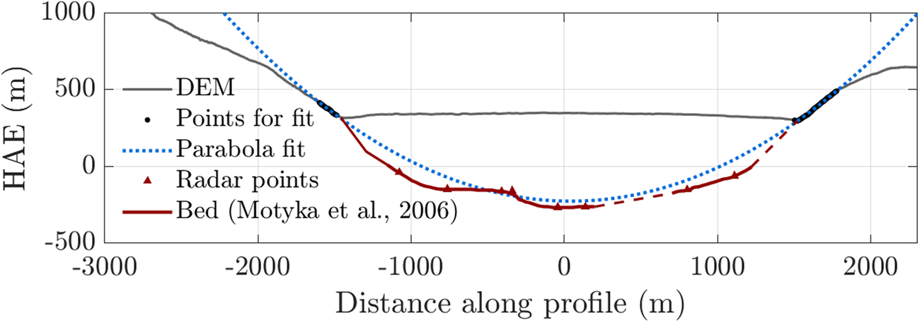
The thickness of the subglacial sediment package is important for estimating the future evolution of the glacier–sediment system. However, available data do not tell us the total thickness of sediments beneath Taku Glacier, because we have no definitive observations of the mid-valley bedrock surface. Therefore, we calculate a first-order estimate of the bedrock elevation beneath Taku Inlet and the present day Taku terminus by fitting parabolas to valley walls, using only elevation data from areas of exposed bedrock. Parabolas are chosen because they approximate a glacial valley cross section reasonably well (Graf, Reference Graf1970). A DEM paired with a radar survey by Motyka and others (Reference Motyka, Truffer, Kuriger and Bucki2006) (Fig. 3) allows us to test a parabola fit to a Taku Glacier valley cross section, albeit one that may still be soft bedded and thereby underestimates bedrock depth.
Radar cross-section at the location of the 1905 terminus (Motyka and others, Reference Motyka, Truffer, Kuriger and Bucki2006), showing land surface (gray line) and an example of a parabolic fit to estimate bedrock. The parabola (blue dotted line) is only fit using parts of the DEM profile that have exposed bedrock (black dots). Elevation in height above ellipsoid (HAE).
We chose transects 5 km from the terminus where Taku Glacier narrows into a symmetric U-shaped glacier valley. We also chose transects across Taku Inlet both upriver and downriver of the Taku Glacier terminus. We then interpolated mid-valley bedrock elevations between the upglacier transect and Taku Inlet using a spline surface fit to the bases of the parabolas.
Although subglacial bedrock elevation data is lacking, we are able to determine the thicknesses of sediments deposited after 1890 CE using various surveys. We analyze spatial and temporal variations in the fjord, glacier and sediment geometry along a longitudinal profile (purple line, Fig. 1). We use the USCGS bathymetric surveys to determine the 1890, 1931 and 1952 fjord bottoms, a photogrammetric DEM for the 2005 glacier surface and proglacial surface, a Worldview DEM for the 2015 foreland and ice surfaces, and 2003–2005 and 2014–2016 radar and GPS data for the 2005 and 2015 glacier beds, respectively. The 1937 ice surface is from a USCGS map, and the 1750 ice surface is a reconstruction from Post and Motyka (Reference Post and Motyka1995). Sediment deposition rates in the fjord are determined by dividing the change in fjord bathymetry by the time between measurements. We use the root sum square of the uncertainties of the two surfaces being compared (Table 1), divided by the time between measurements, to yield the erosion rate uncertainty.
3.2 RES surveys
The purpose of repeat RES surveys is to quantify evacuation and deposition of subglacial sediments. Motyka and others (Reference Motyka, Truffer, Kuriger and Bucki2006) performed RES point surveys of the lower study area with a 2–5 MHz monopulse radar transmitter in June 2003, August 2003 and May/June 2004, obtaining 146 individual soundings. To assess changes in the glacier bed, we resurveyed the majority of these points in June/July of 2016. We also surveyed radar transects in the upper study area in 2014, which overlap with radar surveys conducted in 2003–2005 at the 1937 and 1944 terminus locations (Fig. 1a).
For the 2014/2016 surveys, we used a 2.5 MHz monopulse radar transmitter. The dominant source of uncertainty in ice thickness measurements is from picking the start of the bed reflection wavelet on the radargram. The timing of the bed reflection arrival can be determined to within 0.1 μs (corresponding to about 8 m of ice thickness) for every sounding, or 11.3 m (~0.9 m a−1 for our time period) when calculating elevation differences between the two survey periods. We assume a radar wave speed of 168 ± 2 m μs−1 for temperate glacier ice (Motyka and others, Reference Motyka, Truffer, Kuriger and Bucki2006); this results in an additional bed elevation change uncertainty of 4.95 for 300 m thick ice, which is assumed to be a systematic error. Since it is unlikely that the refractive index of Taku Glacier ice has changed between repeat radar surveys, the radar wavespeed should have remained constant, at some value between 166 and 170 m μs−1. We used post-processed precision GPS to determine the glacier surface at all RES locations. Together with the ice thickness this enables us to calculate the absolute elevation of the glacier bed.
3.3 Hydraulic potential
The RES measurements allow us to estimate the piezometric surface (ϕs) of the study area, which aids us in our analysis of the glacier drainage system and thus the possible directions of sediment movement. For these calculations, we assume that the glacier ice is at a constant fraction of flotation and use ϕs = kρig(z s − z b) + ρwg z b, where ρi is the ice density (917 kg m−3), g is the gravitational acceleration, z s and z b are the elevations of the glacier surface and bed, respectively, ρw is the density of freshwater, and k is the fraction of full ice flotation (Shreve, Reference Shreve1972). We also calculate potential surfaces assuming three quarters and one half of flotation. We produce a piezometric surface using a spline fit and use the QGIS software package (QGIS Development Team, 2018) to calculate surface slopes, which together allows us to calculate the hydropotential gradient at every point in the RES survey area.
3.4 Dye tracing and proglacial stream locations
We used dye tracing to test our water drainage assumptions that are based on the piezometric surface. For the dye injection sites, we used boreholes and natural ice surface entrances to the englacial drainage system. We drilled the boreholes to the glacier bed in July/August of 2015 with a hot water drill. The boreholes were drilled near the center of our lower radar survey area and clustered at five different locations, in a cross shape, with a centrally located set of boreholes and additional boreholes located ~200 m away along the axes of the cross (green dots, Fig. 1b). We used the boreholes to install a variety of instruments to study ice dynamics and basal conditions (not discussed here) and to perform three dye tracing experiments. On 30 July 2015, we poured dye into the center borehole. Dye was injected through a hose into the bottom of the East Borehole during the 4 August 2015 experiment, and poured into a surface stream near the center borehole on 6 August 2015. This surface stream flowed into a crevasse and ran south for some distance (at least tens of meters) before dropping into a moulin or englacial channel. A rhodamine detector was installed in a small outwash stream immediately east of the proglacial bulges (Fig. 1b, pink square).
We used 2014–2016 Worldview imagery and a 2005 aerial orthophoto (Truffer and others, Reference Truffer, Motyka, Hekkers, Howat and King2009) to outline the locations of outwash streams on Oozy Flats and the points at which they emerge from Taku Glacier. We quantify relative outwash stream sizes by estimating the channel width from the imagery. From 2014 to 2017, a time-lapse camera was directed over Oozy Flats from the west, which recorded daily scenes at noon.
3.5 DEM differencing
To quantify proglacial deposition and erosion rates, we used 2-m-resolution Worldview DEMs obtained from the Polar Geospatial Center (Porter and others, Reference Porter2018) and dated 6 June 2014, 12 May 2015, 23 September 2015 and 19 May 2016. These DEMs were co-registered using features on dry land adjacent to Oozy Flats that remain stable between scenes. For each DEM, we averaged landmark offsets in the east and north directions using a reference scene, then applied a constant horizontal shift with a remaining horizontal uncertainty of ~ 3 m (the diagonal of one 2 m pixel). A 10-m-wide meadow of lichen in the same area was used to calculate the constant shifts to coregister DEMs in the vertical direction. This spot was chosen as it was flat, stable ground and did not experience significant seasonal changes in vegetation height.
DEM errors are known to be correlated over certain spatial scales. To assess this scale and the subsequent treatment of errors we follow the methodology of Motyka and others (Reference Motyka, Fahnestock and Truffer2010), derived from Rolstad and others (Reference Rolstad, Haug and Denby2009), and define:


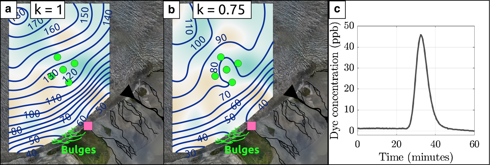
where L is the correlation length (determined by calculating a variogram of the elevation change over the stable lichen patch, and finding its sill height), A c is the equivalent correlation area, σΔZ is the gridpoint elevation uncertainty (the range of the variogram), A is the area of the elevation change and σΔA is the area elevation uncertainty.
Volume error due to the horizontal displacement is $\sim \!10 \percnt$ , found from testing the differencing of DEM pairs, with one DEM shifted by the ~ 3 m horizontal uncertainty (the diagonal of one 2 m × 2 m pixel). A third error component is due to ≤ 0.1 m of buried snow in springtime DEMs (based on observations from March 2015), which causes overestimation of both wintertime deposition and summertime erosion. A 2005 DEM based on photogrammetry (Truffer and others, Reference Truffer, Motyka, Hekkers, Howat and King2009) was also utilized (10 m resolution, with a vertical error of ± 0.65 m).
4. Results
4.1 Taku Glacier profile
Sediments in the Taku Glacier system are reworked in various ways and are eroded and deposited in both subglacial and proglacial environments. Figure 4 shows a time series of five cross sections of the fjord-sediment–glacier system along our study transect (purple line in Fig. 1). The location of the glacier bed in Panel ‘a’ is based on our parabolic best-fits to bedrock. Figure 3 shows such a fit (blue dashed line) to a RES transect (red line) close to the 1905 terminus location (Figs 1 and 4) (Motyka and others, 2006). We find our parabola underestimates the radar depth by ~ 40 m at the valley center. The thickness of 1750–1890 sediment layer in Panel ‘b’ assumes deposition at 1.5±0.5 m a−1 during this time frame. The latter is based on post-1890 deposition rates in Taku Fjord, which range from ~1 to 2 m a−1. The thickness of the sediment layers in succeeding panels was derived from differencing bathymetric data.
Longitudinal profile of Taku Fjord, Taku Glacier terminus, and subglacial/fjord sediments, during (a) 1750; (b) 1890; (c) 1937; (d) 1952; (e) 2005 and (f) 2015. Dotted lines indicate the estimated feature boundaries. Unlined edges or dashed lines indicate the feature boundaries constrained by DEMs, radar surveys and/or USCGS bathymetric surveys. Point radar measurements appear as triangles. The location of this transect is shown in Fig. 1a (purple line).

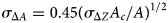
Deposition rates in front of the advancing glacier terminus varied spatially along the glacier profile. Historical deposition rates at the location of the 2015 terminus are as follows: 1890–1937, 0.19±0.05 m a−1; 1937–1952, 1.01±0.09 m a−1 and 1952–2005, 0.60±0.02 m a−1 (Fig. 4f). Deposition rates farther upstream from the 2015 terminus were much higher: at the 1937 terminus, 1.71±0.05 m a−1 from 1890 to 1937; and at the 1952 terminus, 2.88±0.09 m a−1 from 1937 to 1952 (Figs 4c and d). Excavation rates of these sediments after being overridden by glacier ice are described in Motyka and others (Reference Motyka, Truffer, Kuriger and Bucki2006) and in the following section. As of 2020 CE, parts of the 1952–2005 sediment package (turquoise layer in Figs 4e and f), including parts of the proglacial bulges, are still exposed subaerially. The glacier has gradually been overriding these bulges so that only a fraction of their 2002 area still remains exposed (Fig. 5).
Ikonos (top two panels) and WorldView-1 (bottom panel) imagery of Taku Glacier overriding the proglacial bulges. Imagery Copyright 2002, 2010 and 2014, DigitalGlobe, Inc. Solid blue line: 2002 terminus. Dashed blue lines: 2002 bulges.
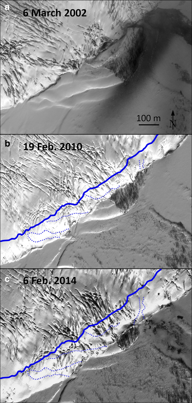
Figure 4f shows that the present-day terminus of Taku Glacier has at least 50 m of sediment to erode through before it can contact the 1890 fjord bottom, which is the minimum possible bedrock depth. However, our parabola fits do not support the 1890 fjord floor being bedrock. Although the parabola-fitting method is a crude approximation, it suggests that the sediment/bedrock interface lies far below the terminus of Taku Glacier. The glacier valley would need to have an unlikely shape for bedrock to be close to the base of the ice at the terminus, with an unexplained bedrock rise in the valley bottom. We estimate the glacier terminus to be 260 m above the 1750 fjord bottom, based on a rate of 1.5 m a−1 of sediment deposition between 1750 and 1890 (Nolan and others, Reference Nolan, Motyka, Echelmeyer and Trabant1995).
4.2 Subglacial sediment transport
We calculated sediment removal rates at two locations in our upper survey area where the radar data from 2014 overlapped with data from 2005. The rate of 2005–2014 glacier bed elevation change at the 1937 terminus position (Figs 2 and 4f) was −2.7 ± 1.3 m a−1. At the 1944 terminus position, excavation rates were too small to be significant (−0.4 ± 1.3 m a−1).
In our lower study area near the 2015 terminus, the rate of change of the glacier bed elevation from 2003/2005 to 2016 ranges from −2.9 to +2.8 m a−1 (Fig. 6), with a measurement uncertainty of ±0.9 m a−1. Sediment reworking shows a clear spatial pattern with excavation and deposition concentrated in distinct areas. The most concentrated sediment removal occurs in a patch 500 m wide (N–S) and at least 800 m long (E–W) just upglacier of Oozy Flats, while deposition dominates in a 1100 m (N–S) by 800 m (E–W) area upglacier of the proglacial bulges (Fig. 6).
Subglacial excavation rates spline fit from repeat point radar survey (actual excavation rate measurements appear in gray-bordered circles; circle size is arbitrary). Proglacial bulges are shown in green. Lines on proglacial fan indicate the historical locations of Oozy Flats outwash streams, colored by date. Colored triangles show the past locations of the largest outlet on Oozy Flats.
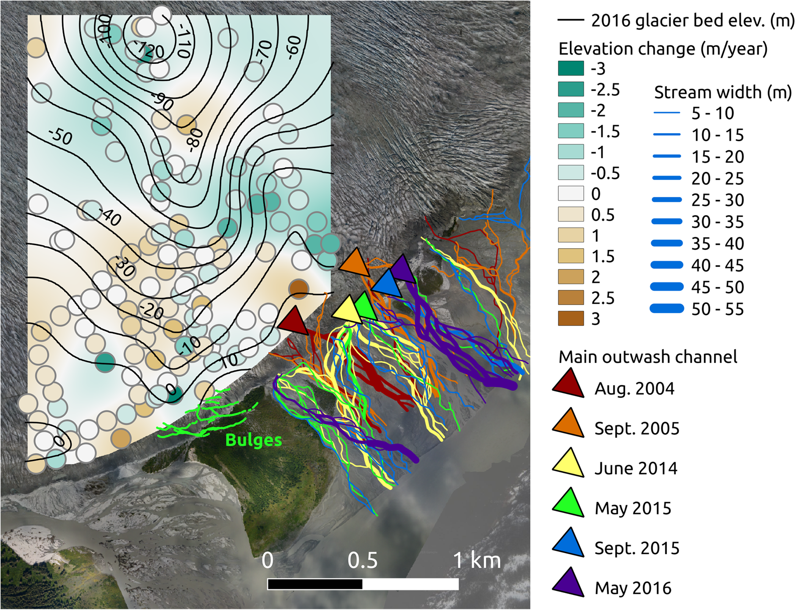
Figure 6 also shows the changing locations of glacier outwash channels. The start of the main outwash channel has largely stayed in the same area of Oozy Flats since 2005. Between June 2014 and May 2016, this main outlet shifted 350 m to the northeast. It moves by abandoning one outlet and occupying an adjacent, smaller outlet. All of these outlets exist just downglacier of the area of concentrated subglacial sediment removal.
We combined the upper and lower radar surveys and used a spline interpolation to produce a DEM for part of the 2015 Taku Glacier bed. The 1890 fjord floor (produced by interpolating between USCGS survey points using a similar spline fit) was then subtracted to show where the glacier has excavated past its 1890 fjord floor (areas of negative value, shown as green lines) and where post-1890 sediments remain (areas of positive value, brown lines). These elevation differences range from negative to positive in the downglacier direction, with values of ~ −140 m 4 km upglacier of the 2015 terminus, to ~ +50 m adjacent to Oozy Flats. The location where the glacier bed has just reached the 1890 fjord floor (white dashed line in Fig. 2) is ~1–2 km from the terminus, closest to the terminus in the subglacial trough area and farthest from the terminus at a location southwest of the subglacial valley wall.
4.3 Subglacial hydrology
Hydropotential surfaces can help us assess potential pathways for water drainage. The piezometric surface assuming full ice flotation is almost completely convex in our lower study area (Fig. 7a), with all contour lines running parallel to the terminus. Using a 0.75 flotation fraction, the piezometric surface contains a concavity in the area of our boreholes (Fig. 7b). This concavity faces towards our rhodamine sensor location (pink square) and not directly towards the major Oozy Flats outwash channel location. Dye poured into the center borehole in the middle of this convexity resulted in an obvious signal at our sensor location. The rhodamine sensor recorded a sudden, 23-minute-long spike in dye concentration with the first arrival appearing ~30 min into the test (Fig. 7c), indicating a fast flow rate (~0.5 m s−1 on average), and comparable to proglacial stream flow at the rhodamine sensor (0.6–0.9 m s−1). Downhole video showed much slower subglacial water flow (0.05 m s−1), indicating that the borehole tapped an active water system, but did not directly intersect a fast channel. Dye from the supraglacial stream and the east borehole did not produce any detectable dye concentration peaks at the rhodamine sensor, indicating that the water was routed elsewhere.
A: Piezometric surface at ice flotation (blue lines; labels in meters of water), September 2015 outwash channel locations (black lines), and erosion rates. Green dots: borehole locations. Pink square: dye concentration monitor location. B: Same as A, but at 75% of flotation. C: Dye concentrations at the monitor in the minutes following dye injection at the center borehole, 30 July 2015. Imagery from 2 August 2015 (Larsen, Reference Larsen2018).
4.4 Proglacial deposition
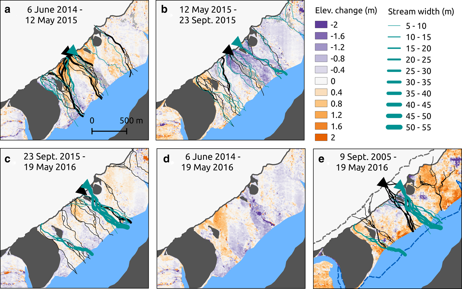
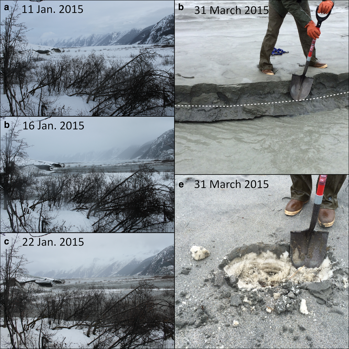
DEM differencing of Oozy Flats shows discrete deposition and erosion events linked to weather and seasonal conditions. Between June 2014 and May 2015, 1.7 +0.2−0.3 × 10⁵ m3 of sediment were deposited over the central and western parts of Oozy Flats (Fig. 8a), with an average deposit thickness of 0.6 m. These deposits are co-located with the braided channels of the main outwash stream from June 2014. Our Oozy Flats time-lapse camera shows a series of deposition events in this area occurring in January 2015 (Fig. 9), concurrent with heavy rainfall. We did not have a functioning rain gauge at the Taku Glacier terminus, but we can use precipitation and air temperature data from a weather station at Juneau airport (~30 km west of the study area) to surmise the evolution of weather conditions during the observed deposition events (Fig. 10).
Results from DEM differencing the Taku proglacial fan. Taku Glacier is in the upper lefthand corner (white area). Dark gray areas are vegetation-covered regions; light gray shows areas of no data. Blue areas show the Taku River in 2016 (a–d) and 2005 (e). Black lines show the outwash stream locations at the beginning of the DEM differencing time period, and teal lines show stream locations at the end of the period. Panel ‘e’ shows the changes from 2005 to 2016, with the 2005 terminus location marked with a dashed gray line, and the 2016 Taku River shore marked with a dark blue dashed line.
Images of the January 2015 Oozy Flats deposition event. Repeat photography (Amundson and others, Reference Amundson, Truffer and Motyka2018) shows Oozy Flats a: prior to b: during and c: after the deposition event. Panel d shows the several decimeters of sediment deposited on top of seasonal river ice. The white line indicates the boundary between river ice and sediment. Panel e shows an area closer to the Oozy Flats time-lapse camera where 1–2 decimeters of sandy sediment was deposited on top of seasonal snow.
Taku Glacier surface elevation and rainfall intensity from 11 to 29 January 2015. Left Y -axis: elevation of a GPS station at the center of the Taku Glacier piedmont lobe (Amundson and Truffer, Reference Amundson and Truffer2018). Right Y -axis: 3-hour precipitation amounts recorded at the Juneau airport. Marker colors show 3-hour average air temperature, with the color scale in the left upper corner of the plot. The location of the GPS station used to record this uplift is shown in Figs 1a and 2.
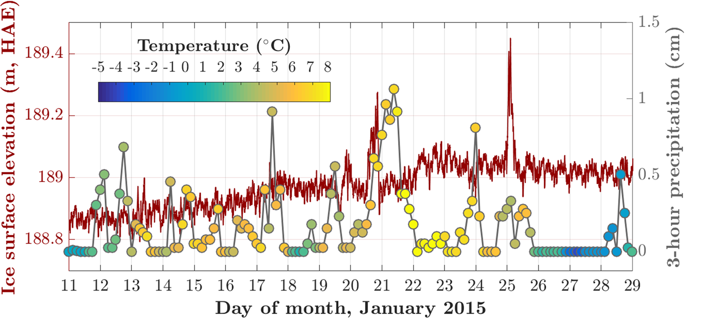
Time-lapse photography of Oozy Flats in January 2015 shows the proglacial channels shrinking and growing and the emplacement of new sediment fans on top of seasonal snow in a vegetated area just in front of the camera and at various locations on Oozy Flats (Fig. 9). Two periods of sediment deposition took place, both occurring during warm and rainy periods (Table 2). During 12–14 January, temperatures rose several degrees, 4 cm of precipitation fell and sediment fans appeared on the southern part of Oozy Flats. Snow covered these fans, then on 20–22 January a major rainstorm occurred wherein 8 cm of rain fell in 48 h at the Juneau airport and an even larger area of Oozy Flats was covered by sediment fans. A sediment fan also appeared in a vegetated area just in front of the camera. During 20 January, the surface of the Taku terminus was uplifted by 31±3 cm, then suddenly dropped back to its pre-storm elevation (Fig. 10). The next time-lapse photograph following the 20 January uplift (taken on 21 January at noon) shows the appearance of the sediment fans. In the following days temperatures dropped and precipitation fell as snow, which covered the sediment fans completely by 29 January. On 31 March 2015, we traveled to Oozy Flats to service the camera and found ~ 0.1–0.3 m thick layers of sediment overlying river ice (Fig. 9d) and seasonal snow (Fig. 9e) in all areas of the January deposition events.
Observations from Oozy Flats timelapse camera
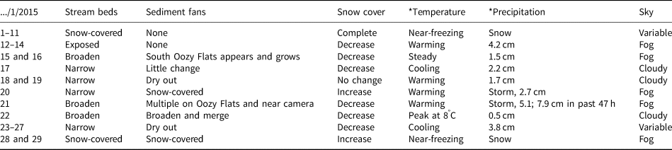
*Juneau Airport weather station.
In the summer of 2015, an area of Oozy Flats, partially overlapping with the sediment deposit mentioned above and bounded by 12 May and 23 September proglacial stream channels, experienced an average of 0.8 m of erosion (Fig. 8b). In total, 2.1 +0.2−0.4 × 10⁵ m3 of sediment was lost in this time period. This error range takes into account the possibility that some of the apparent erosion was due to melt of an entrapped snow layer. This 2015 summer erosion was similar but greater in magnitude than the 2014–2015 depositional event.
Minor changes in Oozy Flats geomorphology occurred in the winter of 2015/2016 (Fig. 8c). There is a small area of deposition around some of the smaller channels that were present in the image from 23 September 2015. The cumulative change over the two years between 6 June 2014 and 19 May 2016 amounts to deposition on western Oozy Flats, no net change over central Oozy Flats, and erosion of eastern Oozy Flats.
Comparing DEMs from 2005 and May 2016, we find that deposition has occurred east of Oozy Flats and in the areas adjacent to Taku River. We find net erosion near the glacier terminus on eastern Oozy Flats, where the main outwash channels tend to be. Western Oozy Flats experienced net sediment deposition. Land surface elevation change along our Figure 4 profile between 2005 and 2015 was insignificant.
In the lower study area, the Taku Glacier surface elevation increased by 7 m, on average, between summer of 2005 and spring of 2015, which is close to the amplitude of seasonal ice surface fluctuations caused by ablation and emergence velocity. Ice surface elevation increase over these 10 years was not uniform and reached ~20 m within a few meters of the terminus. Greater than 1 km away from the terminus and on the west side of the lower study area, the ice surface elevation increase was minimal. Taku Glacier also advanced ~100 m between 2005 and 2015 in the lower study area.
5 Discussion
Our study documents subglacial landform building processes over seasonal-to-decadal time scales, including sediment removal beneath some parts of Taku Glacier and sediment deposition elsewhere. We also witnessed layers of sediment being added to a proglacial outwash fan and stream channels subsequently carving the sediment away. When paired with these observations, changes to proglacial stream locations, dye tracing results and observed erosion patterns allow us to characterize the fluvial sediment transport system responsible for these landforms. The Taku subglacial-proglacial drainage network follows classic temperate glacier seasonal behavior (Hooke and others, Reference Hooke, Wold and Hagen1985; Hodson and Ferguson, Reference Hodson and Ferguson1999; Riihimaki and others, Reference Riihimaki, MacGregor, Anderson, Anderson and Loso2005; Swift and others, Reference Swift, Nienow and Hoey2005; Perolo and others, Reference Perolo, Bakker, Gabbud, Moradi, Rennie and Lane2019), albeit with more winter activity consistant with the wet maritime climate. Our study shows that all of these processes would be capable of continuing for decades in a stable climate, able to keep Taku Glacier in its extended tidewater glacier position, if not for the fact that strong climate forcing has caused Taku Glacier to start a new retreat in 2015 CE (McNeil and others, Reference McNeil2020). Taku Glacier is now transitioning from the advancing phase of the tidewater glacier cycle to the retreat phase.
5.1 Subglacial sediment excavation and hydrology
Our repeat radar surveys show that excavation rates under Taku Glacier are variable over decadal to sub-decadal timescales, and that some areas experience deposition. This is in contrast to the results of Motyka and others (Reference Motyka, Truffer, Kuriger and Bucki2006), who observed sediment removal rates of at least 1.3 m a−1 everywhere within their study area. However, most of their sediment removal rate measurements were net rates over multi-decadal timescales, as they were comparing their 2003/2005 radar data with fjord bathymetry from 1952 and earlier. Our finding of both excavation and deposition occurring on sub-decadal timescales suggests that earlier excavation rates (spanning the years between the 1890–1952 bathymetric surveys and the 2003–2005 radar surveys) were not steady either, and that subglacial sediment was likely being removed and re-deposited over multi-decadal timescales beneath Taku Glacier as it advanced (Fig. 2).
Evidence for glacial excavation down to bedrock appears at the 1905 profile upstream of our study area (Figs 1 and 3). Here, the glacier bottom extends past the bedrock parabola fit and includes asperities that a soft bed would be less likely to support. We therefore suspect that the glacier bed transitions from bedrock to sediment upstream of our study area. If the thinner upglacier sediment package gets depleted, we would expect this transition to move downglacier.
Additional evidence for changing sediment removal patterns is given by the fact that subglacial sediment removal at our lower radar survey area was not concentrated at the bottom of the subglacial trough (Fig. 6). Currently, most sediment removal occurs on the west side of the subglacial trough, while smaller amounts of sediment removal takes place on the east side, and deposition occurs on the shallow south end of the trough. This area is close to the location of the main proglacial outwash channel from 2005 to 2016. We interpret that a subglacial channel occupies the high-excavation-rate area during the summer (when the subglacial drainage system is efficient), and that it also opens sporadically in winter after large snow melt or rainfall events. Our dye tracing experiment confirms a divergent, efficient drainage system in summer. As discharge increases over the melt season, less sediment is supplied to Oozy Flats than is transported away and net proglacial sediment removal results. We return to this point below.
The concentrated excavation patterns and the relatively unchanging location of the main outwash channel indicates that the general location of the subglacial channel is steady, at least over sub-decadal timescales. However, that does not preclude complex seasonal behaviors. Vore and others (Reference Vore, Bartholomaus, Winberry, Walter and Amundson2019) found rapid changes in glaciohydraulic tremor frequency content and signal provenance related to water flow at many locations on Taku Glacier, including in the vicinity of the lower study area and higher up from the glacier terminus. Changes in the locations of channel obstructions and the relative water flux through neighboring channels would explain this observed signal variability. Our data suggest that such changes do indeed occur in the lower study area. Satellite imagery of Oozy Flats shows that the relative sizes of outwash channels change throughout the year without the outlet locations changing significantly (Fig. 6), suggesting that the main subglacial channel meanders as a function of subglacial sediment removal and deposition. These changes in the subglacial hydrological system are probably accompanied by changes in the piezometric surface in the lower study area, so that using a constant flotation fraction to calculate hydropotential might be problematic. Nevertheless, it can be instructive to investigate the constant flotation piezometric surface. Borehole measurements in the study area indicate that water pressure is always greater than an ice flotation fraction of 0.5 (Truffer, Reference Truffer2018). This makes sense, because the retrograde nature of the glacier bed places a constraint on minimum hydraulic head, which has the piezometric surface as a horizontal plane at sea level. From 2–7 August 2015, borehole flotation fraction values averaged ~0.7 and ranged between 0.5 and 0.9. The full flotation piezometric surface in 2016 does not place very strong controls on the location of a subglacial channel, as the piezometric surface is convex and has no valley shapes that would concentrate water (Fig. 7a). If we assume a 0.75 flotation fraction (Fig. 7b), water is generally routed along the subglacial trough to exit just to the east and west of the bulges. Water from all boreholes would take the same path in the 0.75 flotation fraction scenario, which is inconsistent with our dye tracing results. The 0.5 flotation fraction surface is unrealistic because it does not allow drainage of water to the terminus. Our equipotential lines must predominantly follow the ice surface geometry (as they do at full flotation) in order for water from the center and east boreholes to travel in diverging directions.
There is no strong correlation between hydrologic potential gradient and sediment removal rates (Figs 7a and b) over all flotation fractions (0–1). Therefore, we propose that flotation fraction values must not be constant, but vary spatially over the lower study area, so that routing of water at the glacier bed is influenced by factors other than ice surface and bed topography. This is not a surprising result in a constantly evolving drainage system that is driven by large variations in surface melt and precipitation (Shreve, Reference Shreve1972).
Another control on erosion patterns may be the materials over which Taku Glacier has advanced. We find deposition occurring in the area just upstream of the bulges, for example. This could be due to a lack of large subglacial channels. Indeed, no large drainage channels appear where the terminus abuts the bulges. It may also be possible that the glacier bed near the bulges is more difficult to erode than the surrounding areas. The bulges are composed of silt/sand and cobbles, so perhaps the glacier bed just upstream of the bulges has a similar granulometry, and requires faster water flow to be mobilized than the fine-grained marine sediments found at Oozy Flats and at the base of the boreholes. Increased crevassing upglacier of the bulges suggest more resistive basal stress in this location, providing another hint of differing basal conditions.
5.2 Sediment evacuation and proglacial deposition
Sediment removal efficiency patterns seen at Taku Glacier are unsurprising and reflect processes known to occur at other glaciers (Hodson and Ferguson, Reference Hodson and Ferguson1999; Riihimaki and others, Reference Riihimaki, MacGregor, Anderson, Anderson and Loso2005; Swift and others, Reference Swift, Nienow and Hoey2005; Perolo and others, Reference Perolo, Bakker, Gabbud, Moradi, Rennie and Lane2019), with one difference being that glaciological sediment removal patterns typical of springtime also occur in midwinter at Taku Glacier. The temperate, rainy nature of Southeast Alaska ensures that liquid water is available at the Taku terminus almost year-round. Following large amounts of rainfall in winter and spring, proglacial streams widen and deposit decimeters-thick sediment fans over short time scales (hours or days).
Later in the melt season, sediment evacuation efficiency seems to decrease. Like in winter, large water inputs also occur in the summertime, though DEM differencing shows that little sediment is deposited and erosion dominates. This may reflect expected changes in the sizes and distribution of subglacial conduits resulting in a more efficient drainage network and therefore lower suspended sediment concentrations (Hooke and others, Reference Hooke, Wold and Hagen1985; Swift and others, Reference Swift, Nienow and Hoey2005; Perolo and others, Reference Perolo, Bakker, Gabbud, Moradi, Rennie and Lane2019). Higher water flow also means that there is less opportunity for sediments to be deposited on Oozy Flats before they are washed into the Taku River.
Rapid evacuation of sediments in winter points to a perennial drainage network. After months of low water input in winter, these conduits would have shrunken due to ice creep, encroachment by deforming till and sediment deposition (Benn and Evans, Reference Benn and Evans2010). Midwinter rainstorms would pressurize these conduits, causing ice uplift and greater floodwater access to subglacial sediments. Subglacial sediment access likely decreases later in summer, when channels enlarge and water pressure drops (Hooke and others, Reference Hooke, Wold and Hagen1985). At the same time, proglacial stream discharge increases, resulting in summertime erosion at Oozy Flats.
Higher sediment load may not be the only factor causing higher deposition rates during winter versus summer. During this time, water exiting the glacier leaves a pressurized drainage system behind. We speculate that the sudden depressurization of sediment-laden outwash may promote deposition (Perolo and others, Reference Perolo, Bakker, Gabbud, Moradi, Rennie and Lane2019). During summertime, the pressure drop when water leaves the glacier is likely less severe.
5.3 The future of the thrust moraines
The thrust moraines at Taku Glacier have been the focus of several previous studies (Motyka and Echelmeyer, Reference Motyka and Echelmeyer2003; Kuriger, Reference Kuriger2005; Kuriger and others, Reference Kuriger, Truffer, Motyka and Bucki2006). Kuriger and others (Reference Kuriger, Truffer, Motyka and Bucki2006) provided some quantitative analysis to assess under which conditions they could reactivate. To assess the current favorability for bulge reactivation, we analyze the thrust moraine geometries as of 2015 CE, and find that re-activation is unlikely without Taku Glacier re-advance.
In contrast to the rapid fluvial processes that we recorded at Oozy Flats, we have observed no changes in the proglacial bulges over the past 15 years. Instead of moving along their décollement, the bulges have remained static while the advancing glacier overrides them (Fig. 5). Kuriger and others (Reference Kuriger, Truffer, Motyka and Bucki2006) predicted conditions for reactivation by modeling the bulges using an idealized sediment wedge geometry where thrust fault motion occurs if a critical wedge taper is met, i.e. the sediment wedge is at the minimum thickness to be pushed along the décollement without internal deformation and the force exerted on the wedge by the ice (primarily by loading the wedge) exceeds the resistive force along the basal décollement. Their model follows Davis and others (Reference Davis, Dahlen and Suppe1983) and Dahlen (Reference Dahlen1984) and its glaciological application according to van der Wateren (Reference van der Wateren1995) and Fischer and Powell (Reference Fischer and Powell1998). According to this model, thrust faulting at Taku Glacier can occur if: (i) the wedge steepens, shortening its contact with the basal décollement; (ii) the ice surface steepens, placing more pressure on the sediment wedge and/or (iii) pore water pressure rises, decreasing the effective pressure and hence the frictional resistance at the basal décollement (Kuriger and others, Reference Kuriger, Truffer, Motyka and Bucki2006).
We repeat the analysis by Kuriger and others (Reference Kuriger, Truffer, Motyka and Bucki2006) of the proglacial bulge geometry to assess the likelihood of reactivation of the thrust faults. We use a May 2015 Worldview DEM to determine wedge surface slope and ice surface slope along Kuriger and others’ P–P” transect (coincident with the lower part of the profile that we use to produce Fig. 4), and use the 2016 RES survey to find the glacier bed slope. Our analysis reveals little change in the sediment wedge geometry or the steepness of the ice (Fig. 11).
A cross section of Taku Glacier and its proglacial bulges (close-up of Fig. 4), showing angle calculations and the line fits used (red lines). Also shown are 1994, 2005 and 2016 radar soundings of the glacier bed, shown by blue, black and red points, respectively. Errorbars showing bed position uncertainty follow the same color scheme. Décollement elevation is from Kuriger and others (Reference Kuriger, Truffer, Motyka and Bucki2006). 1994 glacier shape (surface and bed) is from Motyka and others (Reference Motyka, Truffer, Kuriger and Bucki2006). The 2005 ice surface is from a photogrammetry DEM (Truffer and others, Reference Truffer, Motyka, Hekkers, Howat and King2009).
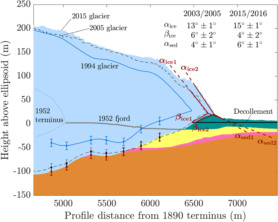
We did not have a method for measuring the effective frictional resistance along the décollement, but we suspect that it is not the controlling factor in bulge reactivation. Sustained, heavy rainfall is common here, and has been observed to cause water to pond on top of the silty clay layer that forms the décollement (Kuriger and others, Reference Kuriger, Truffer, Motyka and Bucki2006), yet in more than a decade of large rainstorms no more motion has occurred.
It appears then that the steepness of the glacier terminus is the controlling factor in moraine re-mobilization. In order for it to steepen, ablation must decrease and/or ice flux to the terminus must increase; thrusting is more likely in winter, when the terminus is steeper and advancing. However, given current climate conditions (McNeil and Baker, Reference McNeil and Baker2019), steepening of the ice front is unlikely to occur.
5.4 Comparisons to surge advances
The proglacial geomorphology of Taku Glacier is quite similar to that observed at other advancing glaciers, particularly in Iceland. The glaciological setting is different there, as advances are caused by sudden surge events, but the same landform building processes can occur in both settings. We have limited information about the Taku Glacier push moraines due to lack of observations during their main formation episodes and due to the continued presence of ice (and in the future, water) hiding the environment upstream of the push moraines. However, such data has been captured in the Icelandic literature. Studies of surging glaciers in Iceland have had the advantage of observing push moraines at the peak of their movement or of observing the deglaciated landscape post-surge (Evans and others, Reference Evans, Twigg, Rea and Shand2007; Benediktsson and others, Reference Benediktsson2008, Reference Benediktsson, Schomacker, Lokrantz and Ingólfsson2010; Korsgaard and others, Reference Korsgaard2015). This Icelandic literature has been discussed in an excellent summary by Ingólfsson and others (Reference Ingólfsson2016).
Many of the features described by Ingólfsson and others (Reference Ingólfsson2016) are similar to those found at Taku Glacier, save for the time scale over which they occurred. Thrust-block moraines in front of the surging glacier Eyjabakkajökull, Iceland formed in a span of 2–6 days (Benediktsson and others, Reference Benediktsson, Schomacker, Lokrantz and Ingólfsson2010), indicating that thrust moraine formation can happen nearly instantaneously. The top speed that Taku Glacier thrust blocks have obtained is unknown, but measurements taken from 6 June 2001 to 1 September 2001 (during their most recent active phase) ranged from 0.09 to 0.15 m day−1, with total bulge motion rate accommodating at least half of the average glacial advance rate of 0.31 m day−1(Motyka and Echelmeyer, Reference Motyka and Echelmeyer2003). Thrusting at Taku occurred as much as 200 m from the glacier front. Eyjabakkajökull thrust blocks also reached ~200 m ahead of the ice margin, but moved two orders of magnitude faster, probably at $\gt 50\percnt$ the advance rate of ~30 m day−1(Benediktsson and others, Reference Benediktsson, Schomacker, Lokrantz and Ingólfsson2010).
The Taku Glacier push moraines occur in only two locations (there was another set of older push moraines to the east of our study area and beyond Oozy Flats, which have since been overridden) and, as discussed previously, could reflect local differences in the glacier bed substrate, as they do in the exposed glacier surge formation in Iceland. Landform types produced by Brúarjökull depended on the granulometry of overridden sediments (Ingólfsson and others, Reference Ingólfsson2016). Coarse-grained sediments with low porewater pressure formed cohesive thrust blocks, resulting in broad, multi-peaked moraines. Fine-grained, high porewater pressure substrate, on the other hand, experienced internal deformation in response to stress and formed narrow single-peaked moraines (Ingólfsson and others, Reference Ingólfsson2016). Kuriger and others (Reference Kuriger, Truffer, Motyka and Bucki2006) found the proglacial bulges at Taku to be composed of dry (4% water content by weight) sand-silt with cobbles overlaying layers of wet (26–35% water content), compact silty clay. The interface between the two units served as the slip plane or décollement for the thrust faults, similar to Brúarjökull (Evans and others, Reference Evans, Twigg, Rea and Shand2007). Because we find the structure of Taku Glacier push moraines to resemble those that formed from coarse-grained sediments at Brúarjökull, it is not unreasonable to surmise that the glacier bed upstream of the Taku Glacier bulges is also coarse-grained.
Unlike at the Taku Glacier bulges, we were able to record very short-term (i.e., days to months) processes at the Oozy Flats outwash plain. This might help shed some light on the formation of the outwash plains in front of Brúarjökull. Korsgaard and others (Reference Korsgaard2015) and Ingólfsson and others (Reference Ingólfsson2016) studied these outwash plains using DEM differencing over decadal timescales (1961–2003), finding sediment deposition rates on outwash fans averaging 0.07 m a−1. By comparison, deposition rates on Oozy Flats at Taku Glacier averaged 0.04 m a−1 from 2005–2015, though our observations of deposition and erosion events showed that the surface elevation change could locally be one order of magnitude faster for short time periods (months), or three orders of magnitude faster for even shorter time scales (days). Perhaps similar events occurred at the Brúarjökull outwash plains, but it is only their modest net contributions to landform building that could be captured using DEMs recorded decades apart.
5.5 The future of Taku Glacier
Taku Glacier still overlies a plentiful sediment reservoir that will allow high sediment mobilization rates for decades to come. If we assume that future excavation rates are 4 m a−1 (the maximum observed by Motyka and others (Reference Motyka, Truffer, Kuriger and Bucki2006)), the glacier will erode down to our estimated bedrock surface in 15, 46 and 86 years at the 1937, 1952 and 2015 terminus locations, respectively. Since we are assuming an upper bound excavation rate, it is probable that the excavation to bedrock will take longer. Even as accumulated sediments under the terminus are exhausted, the loss of available sediments to be mobilized may be partly offset by possible increases in sediment flux from the higher reaches of the glacier, where very large areas of slow bedrock erosion might lead to additional sediment supply (Delaney and Adhikari, Reference Delaney and Adhikari2020). A warming climate would cause increased water flux under the current accumulation zone, increasing water access to sediment in these high areas even as the terminus reservoir is progressively depleted. Increased water flux may also increase bedrock erosion rates where bedrock is exposed, providing additional sediment for transport (Herman and others, Reference Herman, Beaud, Champagnac, Lemieux and Sternai2011, Reference Herman2015). On the other hand, the thinner sediment package upglacier is likely to be depleted over time, which will lead to a downglacier movement of the line that separates a hard from a soft glacier bed.
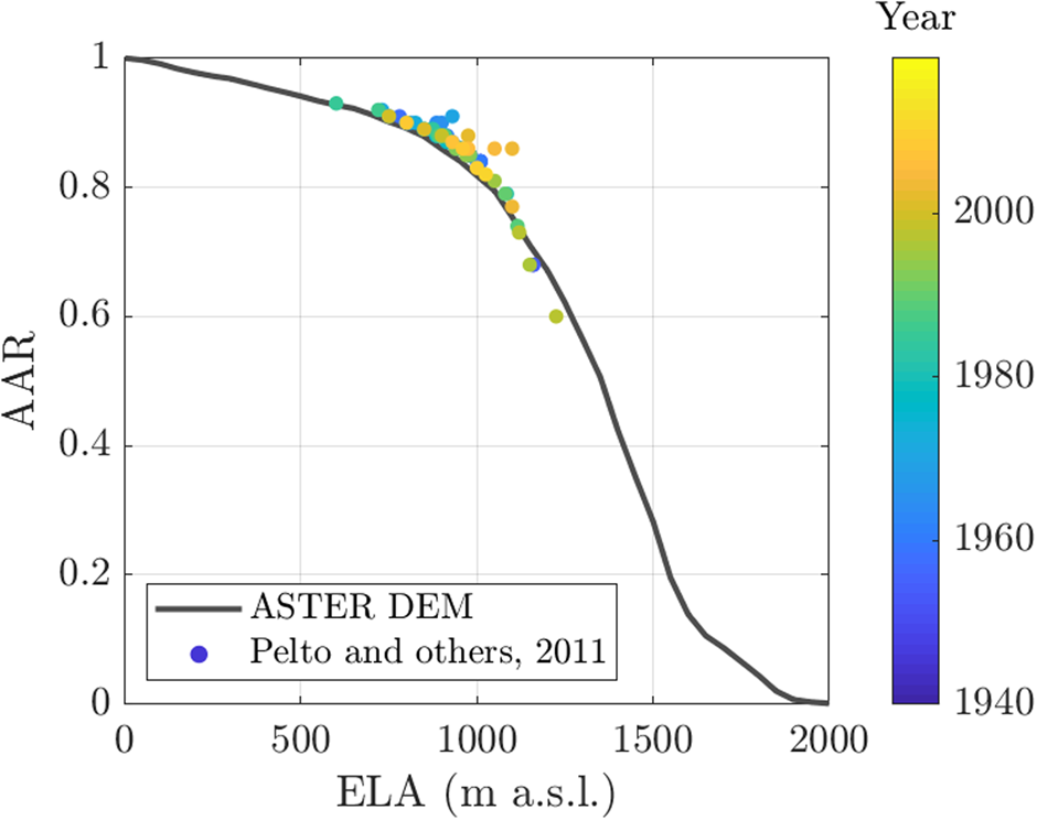
Climate warming has already had a significant impact on Taku Glacier, as evidenced by its mass balance record. Taku Glacier's mass balance was positive through 1989; near zero from 1989 to 2013; and has been consistently negative since 2013, thinning by 6.3 m glacierwide and losing 0.8 km2 in area between 2013 and 2018 (McNeil and others, Reference McNeil2020). Retreat of ~20 m between June 2015 and June 2019 in the lower study area (newly ice-free and vegetated land was observed during a recreational site visit) indicates a long-term retreat may have started. Warming will cause the Equilibrium Line Altitude (ELA) to rise, decreasing the glacier's Accumulation to total Area Ratio (AAR). Calculating Taku Glacier's hypsometry can give us an idea of Taku Glacier's sensitivity to climate warming, as we can tell what impact a rise in ELA will have on Taku Glacier's AAR. The AAR has already dropped significantly since the glacier's most recent rapid advance phase, which occurred in the late-1800s to mid-1900s CE (Nolan and others, Reference Nolan, Motyka, Echelmeyer and Trabant1995). In 1890, the AAR was estimated to be ~0.9, decreasing to 0.83 in the mid-1980s as the glacier increased its ablation area (Post and Motyka, Reference Post and Motyka1995). In more recent years, the AAR has been as low as 0.6. Future warming will decrease the AAR further, at a rate that can be surmised from Fig. 12. Figure 12 describes the sensitivity of Taku Glacier's AAR to changes in climate. This graph shows an inflection point at an ELA of 1000 m, above which the AAR drops rapidly with a rise in the ELA. In recent years, the ELA has been near this inflection point, occasionally exceeding it. Further climate warming will cause significant reductions in the AAR, decreasing by >0.1 for every 100 m rise in the ELA. As the ELA shifts upwards, so too does the start of the zone of basal water flow fast enough to move sediment. Therefore, we do not expect sediment flux to the terminus to drop substantially in the next several decades.
ELA vs AAR from Pelto and others (Reference Pelto, Kavanaugh and McNeil2013) (colored dots) and calculated from a 2016 NED DEM of Taku Glacier (gray line).
Currently the protective proglacial shoal of Taku Glacier has a perennial supply of mobilized sediments to offset erosion because of the position of the terminus which abutts it. However, growing evidence (explained previously) points to imminent glacier retreat. We therefore speculate on what will happen to the terminal shoal once a moat forms between it and the retreating glacial ice.
Parts of the terminus were already in contact with water that accumulates in a moat behind the terminal moraine. Expansion of this moat with continued retreat would create a brackish lake. If ocean water is able to breach the terminal moraine and enter this lake, the retreat will accelerate because ocean water can bring in more heat and increase frontal ablation (Truffer and Motyka, Reference Truffer and Motyka2016). Taku Glacier would then enter a new phase of the tidewater glacier cycle, retreating rapidly until the terminus becomes stabilized by a pinning point or shallow water (Nolan and others, Reference Nolan, Motyka, Echelmeyer and Trabant1995; Post and Motyka, Reference Post and Motyka1995).
Once the terminus retreats into deeper water the glaciofluvial sediment supply to the current terminal moraine will rapidly decline. Without this important sediment source, the present-day Taku Glacier foreland may then suffer net mass loss due to erosion from the Taku and Norris Rivers. In an over-deepened basin and without a pinning point, it is unlikely that Taku Glacier will form a new proglacial shoal to slow the retreat (Eidam and others, Reference Eidam2020). The nearest most likely pinning point is in the vicinity of the 1890 terminus location (~7 km from the 2015 terminus) where the glacier valley narrows and undergoes a sharp turn. Upstream from the proglacial shoal, the bed of Taku Glacier does not rise above sea level again for ~40 km (Nolan and others, Reference Nolan, Motyka, Echelmeyer and Trabant1995). Subglacial sediments farther upstream will eventually become exposed to the calmer marine environment as retreat continues. Without a glacial ice cover, subglacial sediment topography will be quickly buried by marine sediments.
6. Conclusions
During Taku Glacier's advance, four consecutive sedimentary processes occur: (i) glacial outwash sediments and Taku River sediments are deposited on the fjord floor in front of the advancing terminus; (ii) the glacier advances over these fjord sediments and begins to erode them; (iii) the sediments eroded by the glacier are re-deposited onto the proglacial moraine and (iv) proglacial moraine sediments are carried away from the system by adjacent Norris and Taku Rivers as the moraine becomes subaerial and progrades into these river channels.
Landform building processes at the Taku Glacier terminus will remain vigorous with plentiful sediment transport in the foreseeable future. However, the location of these processes will change if the Taku Glacier terminus moves up-valley in response to a warming climate. The continued growth of the 2015 CE terminal moraine is in jeopardy as glacial retreat will make it impossible for glacial sediments to reach the moraine. Fluvial sediment removal is then likely to become the dominant sedimentary process at the moraine, which currently forms a barrier between the glacier and Taku River and Taku Inlet. Erosion of this barrier could then lead to a rapid calving retreat.
In this study, we observed subglacial and proglacial landform building in action and were able to make some inferences about the drainage systems that cause it. We found that subglacial channels shift over decadal timescales but are relatively stationary at sub-decadal timescales. The position of the subglacial channel system draining to Oozy Flats seems to be influenced more by proglacial landforms that Taku Glacier has overridden than the geometry of the calculated piezometric surface. Sediment mobilization occurs in the summer as well as during jökulhlaup-like events triggered by winter rainstorms. Deposition as well as sediment removal occur under the glacier, reworking subglacial topography. The proglacial fan experiences high rates of deposition and erosion on subannual timescales, though it changes little over longer timescales. This indicates that sediment in the Taku Glacier system has been always in transit, moving from the subglacial environment to the proglacial fan, then (via erosion by proglacial streams and by the Norris and Taku Rivers) to the marine environment.
Acknowledgements
We are grateful to Doug Brinkerhoff for radar and borehole fieldwork, Dale Pomraning for his assistance with field work and his building of our borehole instrumentation, and William Dryer for field assistance. We wish to thank Coastal Helicopters and CH2MHILL Polar Services for logistical support, and the Polar Geospatial Center at University of Minnesota for DEMs. Ali Graham, Ian Delaney, and an anonymous reviewer provided valuable feedback allowing us to improve this paper. This project was funded by the U.S. National Science Foundation (NSF-PLR grants 1 304 899 and 1 303 895) and supported in part by a University of Alaska Fairbanks Center for Global Change Student Research Grant with funds from the Cooperative Institute for Alaska Research. We also thank the T'aak Kwáan’ Tlingits, whose ancestral lands lie along the Taku River and Inlet.
Contribution statement
M Truffer, JM Amundson, CL Larsen, and RJ Motyka designed this study. JM Zechmann carried out the data analysis and led the writing. All authors participated in field work, completed parts of the data analysis, and contributed to the editing of the paper.


 Open access