


Impact Statement
The insights gained from this study extend beyond building energy management, offering a broader evaluation of Time-Series Foundation Models (TSFMs) when applied to domains they were not explicitly trained on. Our findings serve as a critical indicator of TSFMs’ strengths and limitations in out-of-domain generalization. Their ability to extract zero-shot representations proves remarkably effective, highlighting their potential for applications requiring automated feature learning and transferability across diverse time-series tasks. However, their reliance on univariate forecasting and the inability to leverage covariates effectively underscore fundamental architectural limitations. The inability of current strategies to integrate external factors signals the need for new model designs that can better capture contextual dependencies. By demonstrating these gaps, this work informs future developments in TSFMs, guiding research toward more adaptable, scalable, and context-aware models for both energy management and broader time-series applications.
1. Introduction
Building energy management (BEM) often requires accurate results from a variety of computational tasks performed on time-series data, such as forecasting, classification, data imputation, and others. Traditionally, these tasks are addressed using a variety of approaches, including statistical models (Zhao and Magoulès, Reference Zhao and Magoulès2012), machine learning (Seyedzadeh et al., Reference Seyedzadeh, Rahimian, Glesk and Roper2018), and physics-based techniques (Sun et al., Reference Sun, Haghighat and Fung2020; Chen et al., Reference Chen, Guo, Chen, Chen and Ji2022). However, heterogeneity—in terms of structure, operation, and environmental conditions—between buildings necessitates the development of task-, modalityFootnote 1-, and building-specific models (Blum et al., Reference Blum, Arendt, Rivalin, Piette, Wetter and Veje2019). This fragmented approach introduces challenges in generalizability, limiting the broader applicability of the resulting solutions.
Time-Series Foundation Models (TSFMs) have recently emerged as a promising approach for achieving generalizability across datasets and tasks, drawing inspiration from the transformative success of Large Language Models (LLMs). Most TSFMs adopt the well-known transformer architecture, incorporating modifications to better accommodate the characteristics of time-series data. These models are typically pretrained on a diverse corpus of time-series datasets, enabling them to perform tasks such as forecasting and anomaly detection in a zero-shot manner. Pioneering examples, such as MOMENT (Goswami et al., Reference Goswami, Szafer, Choudhry, Cai, Li and Dubrawski2024 and TimesFM (Das et al., Reference Das, Kong, Sen and Zhou2024), aim to demonstrate generalization across multiple datasets and modalities. Unlike the conventional definitions of foundation models (Bommasani et al., Reference Bommasani, Hudson, Adeli, Altman, Arora, von, Bernstein, Bohg, Bosselut and Brunskill2021), the vast majority of the TFSMs proposed so far are not designed to generalize to previously unseen tasks. They are, instead, designed to generalize to new data sources of previously seen modalities, and, in some cases, to new modalities that can be represented as time series—while remaining constrained to a fixed set of tasks (Baris et al., Reference Baris, Chen, Dong, Han, Kimura, Quan, Wang, Wang, Abdelzaher, Bergés, Liang and Srivastava2025).
Though TSFMs may not yet offer the level of generalizability expected from true foundation models, we have yet to empirically and systematically evaluate their ability to perform beyond the limits of what they were designed for and trained on. In this work, we aim to provide a multifaceted zero-shot evaluation of pretrained TSFMs for various building energy management tasks. First, we analyze the generalizability across datasets and modalities for zero-shot univariate forecasting in two key contexts for predictive building management: electricity usage and indoor air temperature. This initial assessment by the authors served as inspiration for the present manuscript, after results were presented at a conference (Mulayim et al., Reference Mulayim, Quan, Han, Ouyang, Hong, Bergés and Srivastava2024). The choice of univariate forecasting for the initial analysis was due to the fact that most TSFMs are only designed to perform univariate forecasting. As a first extension to that early work, in this paper, we examine the covariate utilization of TSFMs, given the dependence of BEM tasks on external factors. Specifically, we investigate the modeling of building thermal behaviors by comparing the forecasting performance of TSFMs with covariates against univariate predictors and conventional thermal modeling approaches. These comparisons are conducted across various prediction horizons to assess their efficacy under different forecasting requirements. Third, we investigate their performance on extracting meaningful representations in a zero-shot setting for classification tasks. Our analysis centers on two distinct classification challenges: appliance classification and metadata mapping. Lastly, we conduct a robustness analysis to understand the details of how TSFMs make decisions. We specifically analyze the model’s: (1) stability under different performance metrics, and (2) adaptability to various operational conditions. For this analysis, we again focus on univariate forecasting, as it remains the primary task supported by existing TSFMs.
Our evaluation of TSFMs reveals the following five key findings: First, in terms of generalizability, TSFMs exhibit strong performance on datasets they were exposed to during pretraining (PT) but struggle with unseen data, particularly when compared to statistical models. While some TSFMs can generalize to new electricity datasets with marginal improvement over statistical methods, their performance on unfamiliar modalities, such as indoor air temperature, is inconsistent—surpassing statistical models for longer forecasting horizons but underperforming for shorter ones. Second, covariate utilization does not enhance TSFM performance, likely due to their training being predominantly univariate; in contrast, traditional methods, optimized for autoregressive forecasting, maintain an advantage regardless of covariate inclusion. Third, regarding representations, Chronos and MOMENT demonstrate the ability to generate meaningful embeddings without dataset-specific training, achieving performance superior to deep-learning-based classifiers but remaining inferior to nonparametric optimization methods, highlighting the considerable potential of pretrained TSFMs in zero-shot classification. Fourth, stability analysis reveals that TSFM performance is highly metric-dependent, with models trained to mimic data distributions better preserving temporal patterns and peaks, whereas those optimized for minimizing magnitude-based errors perform better on root mean square error (RMSE) evaluations, emphasizing the importance of aligning model selection with specific task objectives. Finally, our adaptability analysis shows that TSFMs exhibit varying strengths depending on building operational conditions—some models perform better under occupied settings with more dynamic patterns, while statistical models excel under unoccupied, cyclic conditions where energy consumption follows repetitive trends. These findings underscore both the promise and limitations of TSFMs for BEM, highlighting areas where further advancements are needed to improve their robustness and applicability.
The remainder of this paper is structured as follows: Section 2 provides an overview of existing TSFMs, laying the foundation for our analysis. Sections 3 through 6 follow a unified structure, each presenting datasets, models, experimental setup, metrics, and results to systematically evaluate TSFMs across different tasks. Specifically, Section 3 investigates univariate forecasting, assessing TSFMs in a conventional predictive setting. Section 4 extends this examination to forecasting with covariates, evaluating whether incorporating additional contextual information enhances performance. Moving beyond forecasting, Section 5 explores classification tasks, analyzing TSFMs’ ability to generate meaningful representations without explicit task-specific training. Section 6 shifts focus to robustness analysis, examining how TSFMs capture temporal dynamics and identifying conditions where they underperform. Section 7 synthesizes these findings, discussing their broader implications, and finally, Section 8 concludes the paper with key insights and suggested future research directions.
2. Background
2.1. Existing TSFMs
A foundation model is defined as “any model that is trained on broad data (generally using self-supervision at scale) that can be adapted (e.g., fine-tuned) to a wide range of downstream tasks” (Bommasani et al., Reference Bommasani, Hudson, Adeli, Altman, Arora, von, Bernstein, Bohg, Bosselut and Brunskill2021). Following that definition, we would expect TSFMs to generalize to a wide range of downstream tasks, yet most existing TSFMs either solely focus on forecasting (Ansari et al., Reference Ansari, Stella, Turkmen, Zhang, Mercado, Shen, Shchur, Rangapuram, Arango, Kapoor and Zschiegner2024; Das et al., Reference Das, Kong, Sen and Zhou2024; Rasul et al., Reference Rasul, Ashok, Williams, Ghonia, Bhagwatkar, Khorasani, Bayazi, Adamopoulos, Riachi, Hassen, Biloš, Garg, Schneider, Chapados, Drouin, Zantedeschi, Nevmyvaka and Rish2024), require dataset-specific training (Dong et al., Reference Dong, Wu, Zhang, Zhang, Wang and Long2023; Jin et al., Reference Jin, Wang, Ma, Chu, Zhang, Shi, Chen, Liang, Li, Pan and Wen2024), or can only perform a fixed range of tasks (Garza et al., Reference Garza, Challu and Mergenthaler-Canseco2024; Goswami et al., Reference Goswami, Szafer, Choudhry, Cai, Li and Dubrawski2024). Given these constraints, understanding the architectural choices and design trade-offs of current TSFMs is essential for evaluating their generalization potential. As this is a nascent and evolving field, with most models released in 2024, we first review existing TSFMs and summarize their architectures and attributes. Figure 1 shows the overview of the TSFM architecture studied in this work.
Overview of different TSFM architectures. The task-specific heads enable adaptation to different downstream tasks. The encoder generates latent representations, while the decoder autoregressively predicts future tokens. The encoder and decoder architectures studied in this work are transformer-based but can be generalized to other model architectures.

Encoder-based architecture. MOMENT uses an encoder and lightweight prediction heads as backbone (Goswami et al., Reference Goswami, Szafer, Choudhry, Cai, Li and Dubrawski2024). The model tokenizes input data using fixed-length patches and employs transformers (Vaswani et al., Reference Vaswani, Shazeer, Parmar, Uszkoreit, Jones, Gomez, Kaiser and Polosukhin2017) for prediction, incorporating reversible instance normalization for rescaling and centering time series. This approach allows MOMENT to be adapted to various downstream tasks. Chronos (Ansari et al., Reference Ansari, Stella, Turkmen, Zhang, Mercado, Shen, Shchur, Rangapuram, Arango, Kapoor and Zschiegner2024) uses the T5 architecture (Raffel et al., Reference Raffel, Shazeer, Roberts, Lee, Narang, Matena, Zhou, Li and Liu2020) for probabilistic forecasting. Chronos tokenizes time-series values using scaling and quantization and then trains existing transformer-based language model architectures on these tokenized time series using cross-entropy (CE) loss. SimMTM (Dong et al., Reference Dong, Wu, Zhang, Zhang, Wang and Long2023) uses an encoder-based transformer architecture with modules for masking, representation learning, similarity learning, and reconstruction. Uni2TS (Woo et al., Reference Woo, Liu, Kumar, Xiong, Savarese and Sahoo2024) utilizes encoder-only transformers for multivariate time series, handling different patches and variates. It addresses cross-frequency learning, covariate handling, and probabilistic forecasting. UniTime (Liu et al., Reference Liu, Hu, Li, Diao, Liang, Hooi and Zimmermann2024) uses an encoder-based transformer, incorporating semantic instructions through a language encoder to handle domain confusion.
Decoder-only architecture. LagLlama (Rasul et al., Reference Rasul, Ashok, Williams, Ghonia, Bhagwatkar, Khorasani, Bayazi, Adamopoulos, Riachi, Hassen, Biloš, Garg, Schneider, Chapados, Drouin, Zantedeschi, Nevmyvaka and Rish2024) uses the Llama architecture (Touvron et al., Reference Touvron, Lavril, Izacard, Martinet, Lachaux, Lacroix, Rozière, Goyal, Hambro, Azhar and Rodriguez2023) for multivariate time series with a focus on probabilistic forecasting. It employs lag features, data augmentation, and the conventional Llama architecture for robust predictions. TimesFM (Das et al., Reference Das, Kong, Sen and Zhou2024) model employs a decoder-based transformer for multivariate time series, processing patches through residual blocks to generate tokens for forecasting.
Others. TimeLLM (Jin et al., Reference Jin, Wang, Ma, Chu, Zhang, Shi, Chen, Liang, Li, Pan and Wen2024) reprograms an embedding-visible language foundation model, such as Llama and GPT-2 models, for univariate time-series forecasting by transforming data into a text format suitable for language models. TimeGPT (Garza et al., Reference Garza, Challu and Mergenthaler-Canseco2024) leverages a transformer-based architecture. TimeGPT also deals with missing data, irregular timestamps, uncertainty quantification, fine-tuning, and anomaly detection.
Table 1 summarizes the attributes of the above models. Zero-shot means whether models can make predictions without any fine-tuning, or they are available without the need for training. We observe that most of these models cannot handle covariates or irregular time-series data (i.e., sampling rate varies over time). Although such attributes do impact building operations, due to limited model availability, in this paper, we only focus on the six models with zero-shot abilities and making univariate predictions.
Comparison of TSFM attributes

2.2. Investigating TSFMs in the building domain
Leveraging language models for energy load forecasting. Although they did not utilize TSFMs, Xue and Salim (Reference Xue and Salim2023) introduced a novel approach to energy load forecasting that leverages language models by transforming numerical energy consumption data into natural language descriptions through prompting techniques. Rather than fine-tuning, their method relied on pretrained transformer-based models—BART, BigBird, and PEGASUS—combined with an autoregressive generation mechanism to iteratively predict future energy loads across multiple horizons. Experimental results on real-world datasets demonstrated that language models, when prompted effectively, could outperform traditional numerical forecasting methods in several cases, highlighting their potential to capture complex temporal dependencies and generalize to new buildings without additional training.
Improving TSFM performance in building energy forecasting. Park et al. (Reference Park, Germain, Liu, Wang, Wichern, Koike-Akino, Azizan, Laughman and Chakrabarty2024) investigated the use of TSFMs for probabilistic forecasting in building energy systems, evaluating models such as Uni2TS, TimesFM, and Chronos on real-world, multi-month building energy data, including Heating Ventilation and Air Conditioning (HVAC) energy consumption, occupancy, and carbon emissions. Their findings indicated that while zero-shot TSFM performance lagged behind task-specific deep learning models, fine-tuning substantially improved accuracy, in some cases reducing forecasting errors by over 50%. These results suggest that fine-tuned TSFMs can outperform conventional deep forecasting models, particularly in their ability to generalize to unseen tasks.
Similarly, Liang et al. (Reference Liang, Deng, Xie, He and Wang2024) examined the adaptation of similar TSFMs for building energy forecasting, identifying the limitations of straightforward fine-tuning due to the lack of universal energy patterns across buildings. To address this, they introduced a contrastive curriculum learning method that optimizes the ordering of training samples based on difficulty to improve adaptation. Their experiments demonstrated that this approach enhanced zero-shot and few-shot forecasting performance by an average of 14.6% compared to direct fine-tuning, highlighting the potential of structured adaptation strategies for TSFMs in energy forecasting.
To the best of our knowledge, these are the only existing studies in this domain. Our work differentiates itself by focusing on multiple time-series tasks, including univariate forecasting, forecasting with covariates, and classification, without evaluating fine-tuning performance. Instead, we aim to assess the zero-shot capabilities of TSFMs to determine whether they can offer comparable generalization to existing methods. Additionally, we incorporate building-specific baselines alongside classical statistical models. The goal of this study is not to propose a TSFM-based approach that surpasses existing tools but rather to critically analyze whether TSFMs, as they exist today, can provide sufficient zero-shot generalizability to replicate established forecasting methods.
3. Univariate forecasting
As most existing TSFMs were mainly trained to perform univariate forecasting, we pay special attention to understand their performance in this setting. This analysis aims to provide an initial understanding of how these models perform over longer horizons encompassing seasonal variations and diverse household behaviors, specifically focusing on temperature and electricity consumption.
We should note that temperature and electricity data can have distinct time constants based on the source from which they are collected. Our initial expectation is that Foundation Models (FMs) would perform better for electricity since they have observed a similar phenomenon (i.e., electricity measurements from single households) during training. Though they have also observed the temperature from datasets such as Weather and Electricity Transformer Temperature (Zhou et al., Reference Zhou, Zhang, Peng, Zhang, Li, Xiong and Zhang2021), the phenomena captured in these datasets exhibit different dynamics than indoor air temperature.
Table 2 summarizes the data familiarity and model structures for the studied TSFMs. We use three categories for data familiarity: (1) familiar with the data modality: the model is trained with data from the same modality as the test set; (2) familiar with the dynamics: the model’s training corpus included time-series data generated by dynamical processes similar to that governing the test data; and (3) familiar with the dataset: occurring when the model has been trained on the same dataset, which in our case happens for the University of California Irvine (UCI) electricity dataset (Trindade, Reference Trindade2015) in some models. Table 2 also captures differences in the model architectures and objective functions. It is worth noting that since TimeGPT is a commercial model, its training data are not publicly available.
Data familiarity and model structures

Abbreviations: MSE, mean squared error; NLL, negative log likelihood; CE, cross-entropy.
3.1. Datasets
Before detailing the datasets, we acknowledge that our selection process introduces inherent biases that shape our findings. Our choices were designed to test TSFM generalization across two distinct scenarios: performance on unseen datasets within a familiar modality, and performance on an entirely unseen modality.
For the first scenario, we use two electricity consumption datasets: UCI, which some TSFMs have been trained on, and Smart*, a common benchmark in the community that serves as our unseen test case. For the second, more difficult scenario, we use the widely used public ecobee dataset for its indoor air temperature. While TSFMs have been trained with outdoor temperature data, indoor air temperature represents a novel modality with vastly different time constants and control dynamics. This experimental design allows for a test of generalization to a sensing modality. These three datasets, summarized below, therefore create a structured evaluation of TSFMs.
ecobee DYD dataset: To test the general ability of TSFMs in predicting indoor temperature, we utilized a large publicly available dataset from ecobee (Luo and Hong, Reference Luo and Hong2022). This dataset comprises data from 1,000 houses across 4 US states: California, Texas, Illinois, and New York, sampled at 5-min intervals with a 1 °F resolution during 2017. To ensure statistically significant, yet computationally feasible tests, we selected eight houses with the least number of missing thermostat temperature values from each state, resulting in a total of 32 houses. A starting point was randomly sampled from each month, using the same starting points across models for a deterministic comparison, while resampling starting points for each house to ensure greater time diversity. This approach allows us to capture diverse house behaviors, climates, and seasonal variations. Sampling starting points were mainly necessary because the data duration changes based on varying context windows and prediction horizon values.
UCI electricity data: Similarly, to evaluate the general capability of these models in energy consumption predictions, we used the UCI Electricity Load Diagrams dataset (Trindade, Reference Trindade2015). This dataset, frequently used in previous works for evaluation, provides an opportunity to reconsider the performance rankings of TSFMs using different metrics. The dataset records electricity consumption in Watts for 370 Portuguese clients from 2011 to 2014, sampled at 15-min intervals. We randomly sampled 30 houses in this dataset, and for each season, we sampled a starting point, resulting in 16 starting points for each client. This method ensures a comprehensive evaluation across different seasonal contexts and house specifics.
Smart*: This dataset contains whole-house electricity consumption for 114 single-family apartments for the period of 2014–2016 in kW (Barker et al., Reference Barker, Mishra, Irwin, Cecchet, Shenoy and Albrecht2012), sampled every 15 min. Similar to the previous approach, we randomly selected 30 houses in this dataset and, for each season, sampled four different starting points.
3.2. Models
TSFMs. We test TSFMs that can do zero-shot univariate forecasting, which leaves us with MOMENT, Chronos, TimesFM, TimeGPT, and Lagllama.
Baselines. Consistent with previous studies, we focus on statistical models, which we train in two ways. First, in the PT approach, we train models on a large training set held out from the test data, retraining them for each different sampling rate (Section 3.3). Second, we perform test-time fitting (TTF), where model parameters are calibrated using only $ C $
samples available in the immediate context window. Our baseline models are:
$ C $
samples available in the immediate context window. Our baseline models are:
-
• AutoARIMA , a variant of ARIMA that automates the selection of the optimal parameters for time-series forecasting by evaluating various combinations (Smith, Reference Smith2023), simplifying the configuration process. The parameters (p, d, q), representing the lag order, the degree of differencing, and the moving average window, respectively, are automatically determined by AutoARIMA, attempting an optimal fit to the data.
-
• Seasonal ARIMA (S-ARIMA) extends ARIMA to handle seasonal data patterns, incorporating additional seasonal components: Seasonal Auto-Regressive, Seasonal Integrated, and Seasonal Moving Average (Smith, Reference Smith2023). SARIMA is defined by (p, d, q) for nonseasonal components and (P, D, Q, m) for seasonal components, where m is the number of periods per season.
-
• Best fit curve (BestFit), developed to model data trends through curve fitting, offers flexibility by allowing various functional forms tailored to specific dataset characteristics. In our case, we fit a fifth polynomial function: $ f(t)={at}^5+{bt}^4+{ct}^3+{dt}^2+ et+f $
, where
$ a $
,
$ b $
,
$ c $
,
$ d $
,
$ e $
, and
$ f $
are coefficients determined during the fitting process and
$ t $
represents time.
$ f(t)={at}^5+{bt}^4+{ct}^3+{dt}^2+ et+f $
, where
$ a $
,
$ b $
,
$ c $
,
$ d $
,
$ e $
, and
$ f $
are coefficients determined during the fitting process and
$ t $
represents time.


3.3. Experimental setting
We define the following notations employed throughout this paper:
-
•
$ H $
: Prediction length (number of samples) -
•
$ C $
: Context length (number of samples) -
•
$ {f}_s $
: Sampling interval (minutes) -
•
$ D $
: Context duration (hours), defined as
$ D=\frac{C\cdot {f}_s}{60} $
-
•
$ P $
: Prediction duration, also called Horizon (hours), is defined as
$ P=\frac{H\cdot {f}_s}{60} $


While previous literature typically presents results in terms of the number of prediction steps/samples, we express these intervals in terms of hours since it is (a) more intuitive for electricity and temperature predictions, and (b) more comprehensible, particularly as we resample data to analyze performance across various durations.
We selected each context-prediction duration pair $ \left(D,P\right) $
based on two criteria:
$ \left(D,P\right) $
based on two criteria: $ C<512 $
and
$ C<512 $
and $ H<64 $
. The primary rationale behind this choice is that most models are optimized to make predictions within these limits (Ansari et al., Reference Ansari, Stella, Turkmen, Zhang, Mercado, Shen, Shchur, Rangapuram, Arango, Kapoor and Zschiegner2024; Das et al., Reference Das, Kong, Sen and Zhou2024; Goswami et al., Reference Goswami, Szafer, Choudhry, Cai, Li and Dubrawski2024. During this selection, we considered the sampling rate and resampled to a lower temporal resolution when necessary. We also tested a context window of
$ H<64 $
. The primary rationale behind this choice is that most models are optimized to make predictions within these limits (Ansari et al., Reference Ansari, Stella, Turkmen, Zhang, Mercado, Shen, Shchur, Rangapuram, Arango, Kapoor and Zschiegner2024; Das et al., Reference Das, Kong, Sen and Zhou2024; Goswami et al., Reference Goswami, Szafer, Choudhry, Cai, Li and Dubrawski2024. During this selection, we considered the sampling rate and resampled to a lower temporal resolution when necessary. We also tested a context window of $ D=512 $
with various prediction horizons (
$ D=512 $
with various prediction horizons ( $ P\in \left\{\mathrm{4,6,12,24}\right\} $
), as the models were primarily trained using a context of this length. The context-prediction-sampling rate tuples
$ P\in \left\{\mathrm{4,6,12,24}\right\} $
), as the models were primarily trained using a context of this length. The context-prediction-sampling rate tuples $ \left(D\left(\mathrm{h}\right),P\left(\mathrm{h}\right),{f}_s\left(\mathrm{mins}\right)\right) $
are as follows:
$ \left(D\left(\mathrm{h}\right),P\left(\mathrm{h}\right),{f}_s\left(\mathrm{mins}\right)\right) $
are as follows:
 $$ {\displaystyle \begin{array}{ll}\mathrm{ecobee}:& \Big\{\left(\mathrm{24,4,5}\right),\left(\mathrm{36,4,5}\right),\left(\mathrm{36,6,10}\right),\\ {}& \left(\mathrm{48,6,10}\right),\left(\mathrm{48,12,15}\right),\left(\mathrm{96,12,15}\right),\left(\mathrm{168,24,30}\right),\\ {}& \left(\mathrm{512,4,60}\right),\left(\mathrm{512,6,60}\right),\left(\mathrm{512,12,60}\right),\left(\mathrm{512,24,60}\right)\Big\}\\ {}\mathrm{Smart}\ast \mathrm{and}\;\mathrm{UCI}:& \Big\{\left(\mathrm{48,12,15}\right),\left(\mathrm{72,12,15}\right),\left(\mathrm{96,12,15}\right),\\ {}& \left(\mathrm{48,24,15}\right),\left(\mathrm{72,24,15}\right),\left(\mathrm{96,24,30}\right),\left(\mathrm{168,24,30}\right),\\ {}& \left(\mathrm{512,4,60}\right),\left(\mathrm{512,6,60}\right),\left(\mathrm{512,12,60}\right),\left(\mathrm{512,24,60}\right)\Big\}\end{array}} $$
For the Smart* and UCI datasets, we started with a larger number of horizons due to the original sampling rate of UCI being 15 min. We maintained this rate for the Smart* dataset to ensure a fair comparison between the two datasets. Furthermore, considering common weekly patterns in household behavior, we aimed to test the prediction performance of these models when a week of data is provided to predict the next day. Hence, we introduced an additional tuple (i.e., $ \left(\mathrm{168,24,30}\right) $
) to account for this pattern.
$ \left(\mathrm{168,24,30}\right) $
) to account for this pattern.
3.4. Metrics
We used RMSE to evaluate the performance of each model, in line with previous work in this area (Ansari et al., Reference Ansari, Stella, Turkmen, Zhang, Mercado, Shen, Shchur, Rangapuram, Arango, Kapoor and Zschiegner2024; Goswami et al., Reference Goswami, Szafer, Choudhry, Cai, Li and Dubrawski2024).
3.5. Results
With the goal of understanding the long-term general performance of TSFMs in predicting electricity usage and indoor temperature, we conducted an analysis using three large datasets. Table 3 presents the results for each model, measured by RMSE, while Figure 2 visualizes these results by illustrating the distribution of RMSE values averaged across all duration-horizon pairs. Our findings offer insights into model performance across a diverse range of seasons and household characteristics.
RMSE values for general analysis. The best is bold, and the second best is underscored

a These experiments were completed using versions of these models from June 2024.
b Models that have seen the UCI dataset in their training phase.
Distribution of RMSE values for the three datasets, averaged across varying duration-horizon pairs.

Our first dataset, UCI, as shown in Table 3a, has been incorporated into the training process for several of the TSFMs that we evaluated. Comparing the performance of these models on a familiar dataset to their performance on an unfamiliar dataset provides insight into their ability to generalize based on the learned or memorized dynamics. Three of the four models that have previously seen this dataset during training (Chronos, TimesFM, and MOMENT) are the top three performing ones, particularly for shorter durations. An interesting observation arises with the Uni2TS model, which approaches the performance of the others as the duration increases, though it has not seen this data before. This phenomenon may occur because the data are resampled as the duration increases, resulting in a dataset that differs slightly from the original training data sampled every 15 min. Consequently, Uni2TS manages to close the performance gap. Comparing statistical models with foundation models, we observed that BestFit (TTF) outperforms models that have not been trained on the UCI dataset (TimeGPT and Uni2TS) on $ C=48 $
and
$ C=48 $
and $ 72 $
. Besides, AutoARIMA (TTF) and BestFit (TTF) outperform LagLlama consistently despite LagLlama being trained on the dataset. Conversely, S-ARIMA (PT) is a close second to the best TSFM (TimesFM) for
$ 72 $
. Besides, AutoARIMA (TTF) and BestFit (TTF) outperform LagLlama consistently despite LagLlama being trained on the dataset. Conversely, S-ARIMA (PT) is a close second to the best TSFM (TimesFM) for $ C=512 $
. This result is part of a broader trend observed in our analysis: extending the context window to 512 generally highlights the advantage of modern foundation models over traditional statistical approaches. While shorter contexts sometimes allow statistical models to remain competitive, their effectiveness diminishes as the window grows, and they lose their leading position to TSFMs.
$ C=512 $
. This result is part of a broader trend observed in our analysis: extending the context window to 512 generally highlights the advantage of modern foundation models over traditional statistical approaches. While shorter contexts sometimes allow statistical models to remain competitive, their effectiveness diminishes as the window grows, and they lose their leading position to TSFMs.
Upon switching to the Smart* electricity dataset (shown in Table 3b), we observe a shift in comparative model performance. It is important to note that the number of steps is not strictly different for shorter and longer durations, as we resample the data for longer durations. Thus, performance discrepancies can be attributed solely to the behavioral characteristics during those durations. Evaluated on the Smart* dataset, Chronos loses its leading position to TimesFM. MOMENT and TimeGPT are comparable in terms of absolute performance, following TimesFM and AutoARIMA. Other FMs are consistently worse than the previous three TSFMs. Specifically, Uni2TS produces forecasting outliers, leading to exceptionally large errors. Regarding statistical models, overall, AutoARIMA (TTF) performs consistently close to the best TSFM (TimesFM), and BestFit (TTF) outperforms three foundation models. The considerably larger errors, compared to those observed with the UCI dataset, are likely due to a combination of two factors: (1) the intrinsic predictability of Smart* is more challenging, as evidenced by the predictions of statistical models (from 200 to 900 Watts), and (2) the limited generalizability of TSFMs, as manifested by the diminishing performance gap between statistical models and TSFMs compared to the UCI dataset. This indicates a limitation in the performance of TSFMs without familiarity with the data set.
The ecobee dataset presents a more diverse set of results (Table 3c), with statistical models outperforming others for shorter durations. As the duration increases, temperature variations tend to smooth out, where TSFMs seem to perform better. Nonetheless, AutoARIMA (TTF) and S-ARIMA (PT) remain competitive, nearly matching the best-performing forecasting models. When comparing MOMENT, TimeGPT, and TimesFM, we find that TimesFM excels in long-duration predictions, whereas MOMENT and TimeGPT perform best during moderate durations where temperature changes are less variable. This nuanced performance indicates the importance of considering duration-specific characteristics when evaluating model efficacy.
3.6. Summary
In summary, as shown in Figure 2, the TSFMs show different levels of performance based on prior exposure to the datasets. In the realm of electricity datasets, though Chronos and TimesFM stand out as the most effective models for a familiar electricity dataset (i.e., UCI), this advantage diminishes with a new dataset (Smart*). In contrast, models like TimesFM and MOMENT demonstrate a robust capability to generalize to novel data, though their performance improvement over AutoARIMA (TTF) and S-ARIMA (PT) is marginal. Specifically, longer context windows tend to amplify the performance gap between advanced foundation models and traditional baselines, with TimesFM emerging as the dominant model. However, it is crucial to note that when performance is averaged across all test cases, we still see minimal performance gaps for models tested on datasets they have not seen in training (see Figure 2). Overall, except for BestFit, performing TTF does not provide significant advantages for statistical models compared to PT. Lastly, statistical models and TSFMs perform closely in indoor air temperature forecasting, with a slight performance gap separating the best statistical models from the TSFMs.
4. Forecasting with covariates
Our previous analysis focused on univariate forecasting, as most existing models are designed specifically for this task. However, BEM inherently relies on multiple covariates, including solar irradiation, outdoor air temperature, and occupancy patterns. Given this dependency, in this section, we evaluate the performance of TSFMs in forecasting with covariates, comparing them against established building thermal modeling baselines.
4.1. Datasets
ecobee + solar. We utilize a subset of the ecobee dataset (Luo and Hong, Reference Luo and Hong2022), augmented with solar irradiance data derived from the National Solar Irradiation Database (National Renewable Energy Laboratory, 2023). This subset was constructed by selecting consecutive 28-day training and 4-day testing periods from the cooling seasons of 1,000 houses, as used in previous studies (Mulayim and Bergés, Reference Mulayim and Bergés2024a; Mulayim and Bergés, Reference Mulayim and Bergés2024b). After filtering for houses with complete and consistent data, the final subset includes 841 houses.
Covariates. Accurately modeling building thermodynamics requires a clear understanding of the covariate structure, which is grounded in fundamental physical principles. Variables such as heat gains from occupants and equipment significantly affect thermal dynamics but are often challenging to measure outside controlled experimental conditions. Alternatively, data from smart thermostats, including heating/cooling duty cycles, solar irradiance, and outdoor air temperature, can be effectively mapped to the parameters of thermal resistance-capacitance (RC) networks, a widely adopted approach for modeling building thermodynamics.
In this study, we predict the target variable $ {T}_t $
(°F), an indoor temperature controlled by the HVAC system at time
$ {T}_t $
(°F), an indoor temperature controlled by the HVAC system at time $ t $
. The covariates utilized for each house are defined as follows:
$ t $
. The covariates utilized for each house are defined as follows:
-
•
$ {T}_{oat}(t) $
: Outdoor air temperature at time
$ t $
(°F), which drives heat exchange between the building and its environment. -
•
$ {Q}_{sol}(t) $
: Global horizontal irradiance at time
$ t $
(
$ W/{m}^2 $
), representing the solar heat gain impacting the building envelope. -
•
$ {\mu}_c(t) $
: Cooling duty cycle at time
$ t $
(unitless, ranging from 0 to 1), indicating the fraction of time the cooling system is active during a given time step.


By formulating these covariates, we align with widely adopted practices in large-scale thermal modeling studies (Vallianos et al., Reference Vallianos, Candanedo and Athienitis2023; Mulayim and Bergés, Reference Mulayim and Bergés2024b). These measurable and practical covariates ensure the applicability of our approach to real-world scenarios, bridging the gap between theoretical modeling and operational deployments.
4.2. Models
TSFMs. We evaluate the forecasting performance of three TSFMs: Uni2TS, TimesFM, and TimeGPT, which are the only models in this study that explicitly support covariate-based predictions. While other models may perform multivariate forecasting, it is important to distinguish that, in many cases, multivariate predictions are merely equivalent to performing multiple univariate forecasts independently, without incorporating the covariate structure into the predictions. The manner in which covariates are utilized varies across the three TSFMs we consider.
First, Uni2TS incorporates covariates by flattening multivariate time series into a single sequence, employing variate encodings and a binary attention bias to disambiguate variates, ensure permutation equivariance/invariance, and scale to arbitrary numbers of variates. Second, though TimeGPT is a commercial and closed-source model, we include it as a baseline for using covariates. Third, unlike the other two methods, TimesFM does not directly perform covariate forecasting. Instead, it follows a two-step approach: first, fitting a linear model to capture the relationship between the time series and its covariates, and then applying TimesFM to forecast the residuals.
Baselines. To evaluate the performance of TSFMs in modeling building thermodynamics, we compare them against three existing approaches. To analyze the informativeness of the covariates, we fit these models to both the data with covariates and the univariate data. Again, we perform TTF to the following models:
-
• Ridge: A ridge regression model, which serves as a representative data-driven baseline for thermal prediction tasks, as shown by Huchuk et al. (Reference Huchuk, Sanner and O’Brien2022)) and Mulayim and Bergés (Reference Mulayim and Bergés2024a)).
-
• Random forest (RF): A machine learning model, which has shown superior performance in a relevant comparison study (Huchuk et al., Reference Huchuk, Sanner and O’Brien2022).
-
• R2C2: A physics-based RC network with two capacitances and two resistances, a well-established approach for modeling thermal behavior by leveraging physical laws (Mulayim and Bergés, Reference Mulayim and Bergés2024b).
4.3. Experimental setting
Both baseline models and TSFMs were tested on the same subset of the ecobee dataset as described above. The initial training dataset for baselines consisted of $ N=672 $
time steps (28 days), while the test set consisted of
$ N=672 $
time steps (28 days), while the test set consisted of $ H=96 $
time steps (4 days). However, given that TSFMs are typically optimized for making predictions where the context window size
$ H=96 $
time steps (4 days). However, given that TSFMs are typically optimized for making predictions where the context window size $ C<=512 $
and specifically, the MOMENT requires
$ C<=512 $
and specifically, the MOMENT requires $ C+H<512 $
. Thus, we made an adjustment where we utilized
$ C+H<512 $
. Thus, we made an adjustment where we utilized $ C=448 $
values from the initial training set for training the baselines and for providing context to the TSFMs. For predictions, we utilized the first
$ C=448 $
values from the initial training set for training the baselines and for providing context to the TSFMs. For predictions, we utilized the first $ H=64 $
values from the test set. This configuration ensures alignment with TSFM design principles while enabling a fair comparison across all models since both baselines and TSFMs have equal information for training/context.
$ H=64 $
values from the test set. This configuration ensures alignment with TSFM design principles while enabling a fair comparison across all models since both baselines and TSFMs have equal information for training/context.
The experimental test is designed around a practical application: Model predictive control (MPC). At any given time $ t $
, the controller is assumed to have perfect historical knowledge of key variables, including
$ t $
, the controller is assumed to have perfect historical knowledge of key variables, including $ T\left(t-511:t\right) $
(thermostat temperature),
$ T\left(t-511:t\right) $
(thermostat temperature), $ {T}_{oat}\left(t-511:t\right) $
(outdoor air temperature),
$ {T}_{oat}\left(t-511:t\right) $
(outdoor air temperature), $ {\mu}_c\left(t-511:t\right) $
(cooling duty cycle), and
$ {\mu}_c\left(t-511:t\right) $
(cooling duty cycle), and $ {Q}_{sol}\left(t-511:t\right) $
(solar irradiance). For future predictions, weather data such as
$ {Q}_{sol}\left(t-511:t\right) $
(solar irradiance). For future predictions, weather data such as $ {T}_{oat}\left(t+1:t+64\right) $
and
$ {T}_{oat}\left(t+1:t+64\right) $
and $ {Q}_{sol}\left(t+1:t+64\right) $
are provided with added Gaussian noise to account for realistic uncertainty in forecasting. The noise addition follows a systematic process to capture temporal variability and cumulative uncertainty. First, a set of standard deviations,
$ {Q}_{sol}\left(t+1:t+64\right) $
are provided with added Gaussian noise to account for realistic uncertainty in forecasting. The noise addition follows a systematic process to capture temporal variability and cumulative uncertainty. First, a set of standard deviations, $ {\sigma}_i $
, is selected, representing different levels of noise intensity. The noise addition follows a systematic process to capture temporal variability and cumulative uncertainty. A set of standard deviations,
$ {\sigma}_i $
, is selected, representing different levels of noise intensity. The noise addition follows a systematic process to capture temporal variability and cumulative uncertainty. A set of standard deviations, $ {\sigma}_i $
, is selected to represent different levels of noise intensity. For each time step
$ {\sigma}_i $
, is selected to represent different levels of noise intensity. For each time step $ t $
into the prediction horizon, noise is sampled as:
$ t $
into the prediction horizon, noise is sampled as:
 $$ {n}_t\sim \mathcal{N}\left(0,t\cdot {\sigma}_i^2\right), $$
Here, $ {n}_t $
represents the cumulative forecast error at time
$ {n}_t $
represents the cumulative forecast error at time $ t $
. This reflects the fact that the sum of
$ t $
. This reflects the fact that the sum of $ t $
independent Gaussian noise terms, each distributed as
$ t $
independent Gaussian noise terms, each distributed as $ \mathcal{N}\left(0,{\sigma}_i^2\right) $
, yields a Gaussian distribution with variance
$ \mathcal{N}\left(0,{\sigma}_i^2\right) $
, yields a Gaussian distribution with variance $ t\cdot {\sigma}_i^2 $
, and therefore a standard deviation of
$ t\cdot {\sigma}_i^2 $
, and therefore a standard deviation of $ \sqrt{t}\cdot {\sigma}_i $
. The sampled noise
$ \sqrt{t}\cdot {\sigma}_i $
. The sampled noise $ {n}_t $
is added to the corresponding weather variable, such as
$ {n}_t $
is added to the corresponding weather variable, such as $ {T}_{oat}(t) $
or
$ {T}_{oat}(t) $
or $ {Q}_{sol}(t) $
, to simulate uncertainty in future predictions.
$ {Q}_{sol}(t) $
, to simulate uncertainty in future predictions.
By varying $ {\sigma}_i $
, the impact of different noise levels on model performance is systematically evaluated, providing insights into the robustness of the controller and the forecasting models under varying degrees of uncertainty. This approach aligns with realistic operational conditions, where future weather predictions are inherently imperfect.
$ {\sigma}_i $
, the impact of different noise levels on model performance is systematically evaluated, providing insights into the robustness of the controller and the forecasting models under varying degrees of uncertainty. This approach aligns with realistic operational conditions, where future weather predictions are inherently imperfect.
The cooling duty cycle $ {\mu}_c\left(t+1:t+64\right) $
, which is determined by an optimization solution (either via sampling or direct convex optimization), represents a controllable variable in the MPC framework. In this study,
$ {\mu}_c\left(t+1:t+64\right) $
, which is determined by an optimization solution (either via sampling or direct convex optimization), represents a controllable variable in the MPC framework. In this study, $ {\mu}_c\left(t+1:t+64\right) $
is assumed to be perfectly known, consistent with the assumptions employed in prior research on building thermal behavior modeling. This assumption is not without effects. In practice, MPC-based controllers output
$ {\mu}_c\left(t+1:t+64\right) $
is assumed to be perfectly known, consistent with the assumptions employed in prior research on building thermal behavior modeling. This assumption is not without effects. In practice, MPC-based controllers output $ {\mu}_c\left(0:{P}_h\right) $
(where
$ {\mu}_c\left(0:{P}_h\right) $
(where $ {P}_h $
is the lookahead window of the MPC controller), but only use the first action in the sequence, and in the next step, regenerate another action set. Thus, in its practical deployment, this resulting action set can change with each step due to the errors in predictions of next states or forecasts of external variables. However, in our evaluation, the output
$ {P}_h $
is the lookahead window of the MPC controller), but only use the first action in the sequence, and in the next step, regenerate another action set. Thus, in its practical deployment, this resulting action set can change with each step due to the errors in predictions of next states or forecasts of external variables. However, in our evaluation, the output $ {\mu}_c\left(t+1:t+64\right) $
is what shall be deployed, no matter the errors being observed throughout the deployment. The true practical use of these forecasters in MPC settings, thus, can only be evaluated via experimental studies, which are out of scope for this work. While our evaluation provides some insight into how the performance would change with respect to covariate prediction error, it does not include the corrective actions that can be taken by the MPC solver at each timestep.
$ {\mu}_c\left(t+1:t+64\right) $
is what shall be deployed, no matter the errors being observed throughout the deployment. The true practical use of these forecasters in MPC settings, thus, can only be evaluated via experimental studies, which are out of scope for this work. While our evaluation provides some insight into how the performance would change with respect to covariate prediction error, it does not include the corrective actions that can be taken by the MPC solver at each timestep.
To evaluate the efficacy of TSFMs, we frame our investigation around two core questions:
-
• Impact of covariates: Does the inclusion of additional covariates enhance the forecasting accuracy of TSFMs compared to univariate approaches for modeling building thermal behavior?
-
• Comparison with traditional models: Can TSFMs outperform conventional modeling paradigms, such as ridge regression and RC networks, in forecasting building thermal behavior?
4.4. Metrics
Unlike baselines that are trained to minimize the error of one-step-ahead predictions, TSFMs are designed to predict multiple time steps ( $ P>1 $
) simultaneously. This capability necessitates a redefinition of the evaluation metric for each question separately to accommodate the architectural features of TSFMs.
$ P>1 $
) simultaneously. This capability necessitates a redefinition of the evaluation metric for each question separately to accommodate the architectural features of TSFMs.
To address the first research question, we assess the accuracy of TSFMs across the entire $ H=64 $
prediction horizon for both univariate and covariate-based settings. The RMSE is used as the primary evaluation metric, calculated over the full prediction interval (shown as RMSEall) to quantify the difference between predicted and actual values.
$ H=64 $
prediction horizon for both univariate and covariate-based settings. The RMSE is used as the primary evaluation metric, calculated over the full prediction interval (shown as RMSEall) to quantify the difference between predicted and actual values.
For the second question, we compare model predictions across common time intervals relevant to building thermal modeling. Prior studies have evaluated forecasting accuracy at intervals ranging from 1 h (Huchuk et al., Reference Huchuk, Sanner and O’Brien2022; Vallianos et al., Reference Vallianos, Candanedo and Athienitis2023; Mulayim and Bergés, Reference Mulayim and Bergés2024a; Mulayim and Bergés, Reference Mulayim and Bergés2024b) to 6 h (Huchuk et al., Reference Huchuk, Sanner and O’Brien2022), and up to 24 h (Vallianos et al., Reference Vallianos, Candanedo and Athienitis2023; Mulayim and Bergés, Reference Mulayim and Bergés2024a). Following this approach, we sample predictions from the TSFMs and baseline models at the 1- (RMSE1st), 6- (RMSE6th), and 24-h (RMSE24th) marks. The RMSE for these sampled intervals is computed across all 771 houses in the dataset, providing a comprehensive evaluation of model performance.
4.5. Results
Impact of covariates. To properly assess the role of external variables, we also evaluated our baseline models in a univariate setting. R2C2 was omitted from this specific comparison, as its physics-informed architecture inherently requires covariates such as outdoor temperature and HVAC duty cycle. The detailed results are presented in Table 4. To better illustrate these findings, Figure 3 is derived from this table and demonstrates the change in performance for five models capable of forecasting both univariately and with covariates. In contrast to the TSFMs, both Ridge and RF exhibit a significant performance improvement with covariates, confirming that these external factors are critical for their forecasting accuracy even in high-noise scenarios. As expected, the value of the information provided by covariates decreases as the noise level increases. This benefit, however, does not consistently extend to TSFMs. The inclusion of covariates does not enhance the forecasting accuracy of TSFMs compared to their univariate counterparts, as evidenced by the red region in Figure 3. For Uni2TS, the addition of covariates results in only marginal changes relative to its univariate implementation. However, as noise levels increase, Uni2TS performance begins to degrade (see Table 4), indicating that while it incorporates covariate information, its sensitivity to uninformative or noisy covariates undermines its robustness. Similarly, TimeGPT performs slightly better when $ {\sigma}_i\le 0.2 $
, but its performance deteriorates beyond that threshold. This suggests that TimeGPT can utilize covariate information effectively under low-noise conditions, yet the introduction of noisy covariates adversely impacts its accuracy, as expected. TimesFM, which employs an ad hoc approach to covariate integration, consistently underperforms, further highlighting that simply including covariates does not guarantee improved forecasting accuracy, especially when the model lacks a principled design for handling multivariate structures.
$ {\sigma}_i\le 0.2 $
, but its performance deteriorates beyond that threshold. This suggests that TimeGPT can utilize covariate information effectively under low-noise conditions, yet the introduction of noisy covariates adversely impacts its accuracy, as expected. TimesFM, which employs an ad hoc approach to covariate integration, consistently underperforms, further highlighting that simply including covariates does not guarantee improved forecasting accuracy, especially when the model lacks a principled design for handling multivariate structures.
Results (in °F) across different noise levels where $ D=448 $
and
$ D=448 $
and $ P=64 $
. Bold and underscored values indicate the lowest and second-lowest error, respectively
$ P=64 $
. Bold and underscored values indicate the lowest and second-lowest error, respectively

a These experiments used the December 2024 release of TimesFM and the June 2024 release of Uni2TS, while tests for the commercial TimeGPT model were conducted using the API version available in January 2025.
Performance impact of adding covariates, measured as the change in overall RMSEall ( $ \Delta $
RMSEall = Univariate—Covariate).
$ \Delta $
RMSEall = Univariate—Covariate).

Notably, even in the absence of noise, the performance of TimeGPT and Uni2TS with covariates shows only slight improvements over univariate forecasters, while TimesFM performs worse. This may stem from the primary training objective of these models being univariate forecasting, underscoring the need for more effective methods to integrate and utilize covariate information in forecasting tasks.
Comparison with traditional models. The results indicate that simple traditional models, such as ridge regression and RC networks, consistently outperform TSFMs in forecasting building thermal behavior, even when trained on the same amount of data as the TSFM context window. This superiority is evident in autoregressive multistep predictions under zero noise conditions (as shown by RMSE6th and RMSE24th), a task for which these baselines were not explicitly designed. Only under increasing noise levels do Uni2TS’s univariate forecasters outperform Ridge and RF for RMSE6th, and TimeGPT achieves better results for RMSE24th. For one-step-ahead predictions (RMSE1st), which are the primary training objective of the baselines, none of the TSFMs come close to their performance. Among the baselines, R2C2 consistently delivers the best one-step-ahead predictions, with minimal performance gaps compared to other traditional methods, underscoring the strength of domain-specific models in capturing the physics and statistical structure of building thermal dynamics.
4.6. Summary
TSFMs, regardless of whether they incorporate covariates, generally struggle to match the performance of traditional baselines. Only under conditions of increased noise do univariate TSFM forecasters begin to outperform the baselines in multistep predictions. Overall, the ability of traditional models to achieve superior performance even with very limited training data suggests that TSFMs still have significant room for improvement before they can consistently surpass these established methods in this domain.
5. Classification
Having demonstrated TSFM’s forecasting capabilities, we now explore its performance on additional tasks. While imputation and anomaly detection can often be treated as natural extensions of forecasting—inferring missing values or flagging outliers based on deviations from predicted signals—classification requires a fundamentally different approach, which is precisely why we chose it.
Unlike forecasting, where a context window directly informs future predictions, classification lacks a straightforward mechanism to provide the model with “example” labels for unseen data. Consequently, zero-shot classification is not inherently possible within TSFMs, as there is no built-in way to infer class labels without supervision. To address this, we leverage MOMENT’s ability to provide representations to extract latent time series embeddings without requiring any labeled training data. These embeddings serve as fixed feature representations, which are then used to train a separate classifier head, such as a support vector machine (SVM), enabling classification without directly finetuning the TSFM itself. To evaluate the performance of this approach, we focus on two distinct yet prevalent classification tasks in BEM:
-
• Appliance classification—identifying which appliance is active based on time series data, and
-
• Metadata mapping—assigning standardized semantic labels (e.g., sensor types, setpoints, or alarms) to diverse building data points.
In the following sections, we describe how TSFM is adapted and evaluated for these classification scenarios.
5.1. Datasets
We leverage two datasets for our experiments on classification:
WHITED. The WHITED dataset (Kahl et al., Reference Kahl, Haq, Kriechbaumer and Jacobsen2016) is a collection of high-frequency energy measurements capturing the start-up transients of 110 appliances, spanning 47 types across 6 regions worldwide. After grouping multiple appliance brands under their respective types, this dataset has 56 unique appliance classes. Data were recorded at 44.1 kHz using low-cost sound card-based hardware, focusing on a 5-s window that captures the transient characteristics essential for tasks like appliance classification and regional grid analysis.
Each sample in the dataset includes voltage and current measurements. Following Kahl et al. (Reference Kahl, Haq, Kriechbaumer and Jacobsen2016)), which reports the best performance when power values are considered, we computed the instantaneous power by multiplying voltage and current to obtain a single feature. Finally, we split the dataset 80/20 into training and testing subsets, resulting in 1,071 training samples and 268 testing samples.
Building TimeSeries (BTS). The BTS dataset (Prabowo et al., Reference Prabowo, Lin, Razzak, Xue, Yap, Amos and Salim2024) comprises over 10,000 time-series data points spanning 3 years across three buildings in Australia. It adheres to the Brick schema (Balaji et al., Reference Balaji, Bhattacharya, Fierro, Gao, Gluck, Hong, Johansen, Koh, Ploennigs and Agarwal2016) for standardization and supports time-series ontology classification—mapping each time series to one or more ontological classes (e.g., sensors, setpoints, or alarms). This multilabel classification problem is challenging due to extreme class imbalance and domain shifts across different buildings, offering a strong benchmark for assessing interoperability and scalability in building analytics.
This dataset requires a multilabel classifier since it features 94 subclasses of labels. Each data point is annotated with:
-
• Positive labels: The true label and its parent classes
-
• Zero labels: All subclasses of the true label
-
• Negative labels: All unrelated labels
Since there is an ongoing public competitionFootnote 2 utilizing this dataset, only a subset is publicly available. We used this subset and split it 80/20 into training and testing, resulting in 25,471 samples for training and 6368 for testing.
One important consideration is the extent to which MOMENT and Chronos have been exposed to data similar to WHITED and BTS during their PT. While MOMENT and Chronos have encountered electricity and temperature data across a range of time constants, the characteristics of these datasets differ significantly from those used in this study. WHITED consists of high-frequency (kHz-level) power measurements captured over a few minutes, whereas these models were primarily trained on lower-resolution datasets such as the UCI electricity dataset, which records household power usage at 15-min intervals. Similarly, the BTS dataset spans multiple sensor modalities—including temperature, alarms, damper positions, and airflow values—most of which are distinct from what these models have seen. The closest match is outdoor air temperature, which aligns more closely with the weather datasets included in the PT corpus of MOMENT and Chronos, while the remaining modalities represent unseen or significantly different data distributions. As a result, evaluating MOMENT and Chronos on WHITED and BTS not only provides insight into their applicability for BEM tasks but also serves as a broader test of their ability to generalize to datasets that deviate from the training distribution.
5.2. Models
TSFMs. Among the TSFMs evaluated, MOMENT and Chronos were the only models capable of performing classification tasks. We utilized them as a zero-shot representation learner in combination with a dataset-specific classification head, as recommended in Goswami et al. (Reference Goswami, Szafer, Choudhry, Cai, Li and Dubrawski2024). Specifically, MOMENT and Chronos were directly applied without retraining to extract latent representations of the time-series data. These latent representations, along with their corresponding class labels, were then used to train an SVM.
Baselines. Based on the performance on University of California Riverside (UCR) classification archive reported in Goswami et al. (Reference Goswami, Szafer, Choudhry, Cai, Li and Dubrawski2024)), we specifically chose the best-performing models from each category and trained each model on our selected classification datasets independently. These baselines are:
-
• TS2Vec (Yue et al., Reference Yue, Wang, Duan, Yang, Huang, Tong and Xu2022) (self-supervised representation learning): Serving as strong baselines in Goswami et al. (Reference Goswami, Szafer, Choudhry, Cai, Li and Dubrawski2024)), TS2Vec employs a two-stage manner to perform classification. At the first stage, it performs contrastive learning to obtain a latent representation of the targeted dataset in a self-supervised manner. At the second stage, a classification head such as SVM is trained on the embeddings learned by the TS2Vec model using class labels.
-
• ResNet (Ismail Fawaz et al., Reference Ismail Fawaz, Forestier, Weber, Idoumghar and Muller2019) (supervised deep learning): As a model demonstrated strong performance consistently among nine deep learning classifiers in Ismail Fawaz et al. (Reference Ismail Fawaz, Forestier, Weber, Idoumghar and Muller2019)), we use the ResNet-18 model as a baseline. The model is trained end-to-end with the classification loss and class labels as supervision.
-
• Dynamic Time Warping (DTW)/Soft-DTW (SDTW) (Cuturi and Blondel, Reference Cuturi and Blondel2017) (supervised nonparametric optimization models): SDTW is a differentiable variant of the traditional DTW algorithm, which is designed to replace the hard minimum operation of DTW with a relaxation. It retains the ability to handle temporal shifts between time series with significant speedup. To perform time-series classification, we combine the distances measured by SDTW or DTW to assign a label based on the majority class of the closest samples. We select
$ K=1 $
in the experiments.To counteract the non-positivity of SDTW, we use the Soft-DTW divergence as the distance metric
$ D\left(\cdot, \cdot \right) $
for the K-nearest neighbors (KNN) classifier:


 $$ D\left(s,\hat{s}\right)=\mathtt{SDTW}\left(s,\hat{s}\right)-\frac{1}{2}\left(\mathtt{SDTW}\left(s,s\right)+\mathtt{SDTW}\left(\hat{s},\hat{s}\right)\right) $$
where $ s $
and
$ s $
and $ \hat{s} $
are two time series.
$ \hat{s} $
are two time series.
5.3. Experimental setting
Our training methodology is structured to accommodate different types of models. (1) For fully supervised models, such as SDTW and ResNet, the training process involves providing the training set with class labels, and the models are trained in an end-to-end manner with categorical cross-entropy loss. (2) For models trained in two stages, like TS2Vec, we first use contrastive learning to train a representation learner without class labels. Subsequently, a separate classification head is trained using class labels. During inference, the time-series data are passed through the frozen representation learner to generate latent embeddings, which are then input into a pretrained SVM to predict class labels. (3) For zero-shot representation learners, such as MOMENT, we directly train the SVM with class labels and time-series embeddings obtained by MOMENT. During inference, the outputs of the MOMENT model are concatenated with the SVM to produce the final predictions.
For the BTS dataset, we employed a multi-output classifier due to its multilabel requirement, as each time series can belong to an arbitrary number of classes simultaneously. Specifically, we employed the binary relevance strategy to adapt the models (ML Zhang et al., Reference Zhang, Li, Liu and Geng2018). For nonparametric optimization models such as SVM and KNN, we trained $ K $
classifiers where
$ K $
classifiers where $ K $
is the number of classes. For deep learning models such as ResNet, we concatenate a sigmoid function to the output logit of the model to generate the probability of classes. To address the input sequence length limitation of MOMENT, we resampled all time series into 512 steps.
$ K $
is the number of classes. For deep learning models such as ResNet, we concatenate a sigmoid function to the output logit of the model to generate the probability of classes. To address the input sequence length limitation of MOMENT, we resampled all time series into 512 steps.
5.4. Metrics
For the WHITED dataset, we use macro precision, recall, and F1 score to ensure equal importance for all appliance types in this class-balanced dataset. While these metrics provide a comprehensive evaluation, accuracy is the primary metric, aligning with its common use in prior work (Kahl et al., Reference Kahl, Haq, Kriechbaumer and Jacobsen2016).
For the BTS dataset, we use micro precision, recall, and F1 score to evaluate performance, as they provide a comprehensive assessment across all classes. Due to the significant class imbalance, the micro F1 score is the most reliable indicator (Prabowo et al., Reference Prabowo, Lin, Razzak, Xue, Yap, Amos and Salim2024). The reason is that the predominance of the negative class makes the accuracy misleading, as models can achieve high accuracy by predicting the majority class without effectively distinguishing minority classes.
5.5. Results
Table 5 summarizes the classification performance regarding accuracy, precision, recall, and F1 score, as well as the computational complexity of each model across the WHITED and BTS datasets.
Results across different metrics and datasets. IBL, instance-based learning; E2E indicates that the model is trained directly using a classification loss in an end-to-end manner; SS-RL, self-supervised representation learning; PT-RL, pretrained representations; SVM/NN, an SVM or a Neural Network (NN) classification head is trained on top of a frozen representation; $ N $
, number of the training samples. Bold and underscored values indicate the best and second-best performance across each metric, respectively
$ N $
, number of the training samples. Bold and underscored values indicate the best and second-best performance across each metric, respectively

a Due to the computational overhead of multilabel classification in Scikit-learn’s SVM implementation, we limit the maximum number of iterations for SVM training to 1000 for the BTS dataset.
Computational complexity. The computational complexity of the models varies significantly based on their training methodology. DTW, SDTW, and TS2Vec exhibit quadratic scaling with the number of training samples due to their reliance on pairwise distance computations—SDTW for DTW calculations and TS2Vec for its contrastive learning framework. In contrast, ResNet scales linearly, as it is trained in a conventional supervised manner using class labels, without the need for pairwise comparisons. The most computationally efficient models in our study are MOMENT and Chronos, as their zero-shot encoders generate embeddings independently of the training sample size. Moreover, the subsequent SVM and Neural Network (NN) classifiers can be trained on a subset of the available samples, further reducing computational demands.
Performance. Performance evaluations indicate that Chronos, when paired with an SVM classifier, achieved state-of-the-art results on the WHITED dataset, even surpassing DTW. However, in the BTS dataset, where the F1 score serves as a more appropriate evaluation metric, Chronos underperformed relative to DTW. Notably, its combination with SVM exhibited significantly weaker performance, likely due to the classifier failing to converge within the imposed limit of 1,000 iterations—an issue attributed to the large scale of the BTS dataset. In contrast, replacing the SVM with an NN classifier substantially improved results, making Chronos the highest-performing approach after DTW and SDTW.
Representation. A key insight from our experiments is that the zero-shot embeddings generated by Chronos consistently outperform those learned through supervised contrastive training in TS2Vec, while MOMENT exhibits comparable performance. Unlike TS2Vec, which requires explicit training on each dataset to extract meaningful feature representations, Chronos and MOMENT generate embeddings directly from their pretrained models without additional fine-tuning. Despite the absence of dataset-specific adaptation, Chronos produces high-quality representations, as evidenced by its strong classification performance when paired with either an SVM or NN classifier. While MOMENT does not match Chronos in representation quality, it still performs on par with TS2Vec, despite the latter’s reliance on dataset-specific training. These findings underscore the effectiveness of TSFMs in capturing universal time-series representations without the need for additional fine-tuning.
Classifier head. Classifier selection remains a critical factor in model performance, as different classifiers exhibit varying levels of effectiveness across datasets. For TS2Vec, MOMENT, and Chronos, our experiments reveal a consistent pattern: SVM performs better on WHITED, while NN performs better on BTS. This is expected, as NNs typically require larger datasets to generalize effectively, whereas SVMs can perform well even with limited training samples. Consequently, NNs tend to outperform SVMs on large datasets, while SVMs may be preferable when data availability is constrained. Overall, the absence of a universally optimal modeling approach aligns with the findings of (Xue and Salim, Reference Xue and Salim2023), which demonstrated that the most effective language models for forecasting varied across different buildings. These observations reinforce the necessity of task-specific and dataset-dependent model/classifier head selection to achieve optimal results.
5.6. Summary
Chronos demonstrates strong zero-shot representation capabilities, achieving competitive performance without requiring dataset-specific training. However, it still remains inferior to statistical models in terms of F1 for large datasets. MOMENT, though inferior to Chronos, has shown comparative performance to deep-learning-based methods that require data-specific training (i.e., TS2Vec). Performance of TSFMs seems to vary considerably based on the classifier used, calling into attention that different classifiers should be chosen depending on the size of the dataset. Despite a possible performance gap for larger and imbalanced datasets (i.e., BTS), Chronos’s drastically lower computational complexity makes it a practical choice for resource-constrained environments, considering the trade-off between efficiency and predictive accuracy.
6. Robustness analysis
This section evaluates model performance across varying conditions and metrics to identify potential failure modes when data characteristics shift. First, we examine how these models generalize to different time scales and forecasting horizons, assessing their adaptability to varying prediction requirements. Second, we analyze edge cases to determine whether they can accurately capture behavioral shifts, such as peak occurrences. Third, we evaluate their performance across alternative metrics beyond RMSE, providing insights into how different training objectives shape their forecasting characteristics. Finally, we assess their robustness under dynamic conditions, such as changes in occupancy patterns. While some of these scenarios may be infrequent, they remain statistically significant and critical for real-world applications.
6.1. Datasets
We specifically seek to test the performance of TSFMs with data subsets representing specific building conditions to understand whether there is significant performance degradation when factors governing the physical system change. To that end, we utilize two sets of data we collected for ~6 months from an experimental testbed with four occupants located in Pittsburgh, PA, which is released alongside the code for all experiments (Quan et al., Reference Quan, Baris and Bergés2025a).
Indoor air temperature. An ecobee thermostatFootnote 3 that takes measurements of 0.1 °F resolution at 5-min intervals was utilized for data collection. Although this dataset comprises 10 temperature sensors, our focus was exclusively on the thermostat temperature. From this dataset, we extracted three subsets based on distinct conditions (Figure 4):
-
• Off: This condition refers to the period when the HVAC system was off for an extended duration, specifically from September 17 to September 29. During this time, although the house was occupied, the HVAC system was not operational due to warm outdoor conditions, resulting in a free-floating thermal environment. The purpose of this period is to facilitate univariate time-series forecasting, as the future values of the time series are less dependent on other covariates due to the absence of heating/cooling input from HVAC.
-
• Heat-occupied: This condition covers the period when the HVAC system was set to heating mode, and the house was occupied. We selected a duration during the winter, from November 2 to December 16, to ensure active heating. During this period, the house followed a schedule defined by the ecobee thermostat, with setpoints of 62 °F during sleep, 64 °F when away, and 68 °F when home. In this condition, we have a more varied temperature pattern as the setpoints change three times during the day in addition to the heat gains by occupants.
-
• Heat-unoccupied: This condition pertains to the period when the HVAC system was in heating mode while the house was unoccupied, from December 17 to January 2. Throughout this period, the house maintained a stable heating setpoint of 60 °F. This condition serves as a test for a more cyclic behavior since the setpoint stays the same for a long period.
Visualization of new empirical data across conditions.

Electricity. A Sense smart meterFootnote 4 was installed in our testbed to collect measurements of active power at 5-min intervals. Although data were collected over a period exceeding 6 months, we extracted two subsets based on distinct occupancy conditions (Figure 4):
-
• Unoccupied: We selected the same unoccupied period as the temperature data, from December 17 to January 2. This condition serves as a test of their ability in more cyclic patterns.
-
• Occupied: This subset consists of data collected from January 3 to February 3 when the house was occupied. When occupied, there are more subtle peaks in the house, and thus it is a good test of their performance on a more varied electricity input.
6.2. Models
We use the same TSFMs and statistical models used for univariate forecasting, as explained in Section 3.2. However, since TTF baselines performed better than PT in most cases, we only present the TTF results for brevity.
6.3. Experimental setting
We conducted experiments that vary across five dimensions:
-
1. Data: {Temperature, Electricity}
-
2. Condition: {Off, Heat-Occupied, Heat-Unoccupied}, {Occupied, Unoccupied}
-
3. Varying context duration
$ D $
(hours): {24, 36, 48,96} -
4. Varying prediction duration
$ P $
(hours): {4, 6, 12, 24} -
5. Varying starting points: We created 10 batches with different starting points for each context-horizon pair by dividing the available data into equal intervals, ensuring each model uses the same set of starting points.


6.4. Metrics
Existing work mainly uses metrics that measure magnitude differences between forecasts and ground truth, such as RMSE, mean absolute scaled error (MASE), and mean squared error (MSE). While these metrics are useful for understanding the quality of predictions, they are intolerant to phase differences, resulting in considerably large values in such cases. Thus, we extend measurement rules to include metrics that quantify the shape similarity between the predictions and the ground truth time series. In that regard, we choose Peak Recall Rate (PRR) and DTW in addition to RMSE to characterize predictions.
PRR. Peak patterns in time series refer to the significant increases in the magnitude of measured variables followed by corresponding decreases, which are common features in air temperature and electricity building data (Braun, Reference Braun1990; Fan et al., Reference Fan, Xiao and Wang2014). Correctly forecasting these peaks offers substantial benefits, including enhanced energy efficiency, cost savings, and improved occupant comfort (Braun, Reference Braun1990). For instance, building control systems can make proactive energy adjustments to balance grid load and participate in demand response programs for financial incentives.
Therefore, we propose to use the PRR as the metric to evaluate models’ ability to forecast peaks and define PRR as follows:
Let $ s $
be the ground-truth time series and
$ s $
be the ground-truth time series and $ \hat{s} $
be the forecasted time series. Let
$ \hat{s} $
be the forecasted time series. Let $ \mathrm{\mathbb{P}} $
be the set of peak indices in
$ \mathrm{\mathbb{P}} $
be the set of peak indices in $ s $
, and
$ s $
, and $ \hat{\mathrm{\mathbb{P}}} $
be the set of peak indices in
$ \hat{\mathrm{\mathbb{P}}} $
be the set of peak indices in $ \hat{s} $
. We calculate the PRR as:
$ \hat{s} $
. We calculate the PRR as:
 $$ \mathrm{PRR}=\frac{1}{\mid \mathrm{\mathbb{P}}\mid}\mid \left\{i\in \mathrm{\mathbb{P}}|\exists j\in \hat{\mathrm{\mathbb{P}}}\;\mathrm{s}.\mathrm{t}.|i-j|\le \tau \hskip0.42em \mathrm{and}\hskip0.42em |{s}_i-{s}_j|\le \varphi \right\}\mid $$
where $ \tau $
and
$ \tau $
and $ \varphi $
are two empirically chosen thresholds to ensure the closeness of the true peak and the forecasted peak in time and magnitude. Typically, we set
$ \varphi $
are two empirically chosen thresholds to ensure the closeness of the true peak and the forecasted peak in time and magnitude. Typically, we set $ \tau =H/20 $
(
$ \tau =H/20 $
( $ H $
is the prediction length) and
$ H $
is the prediction length) and $ \varphi =\sigma $
(
$ \varphi =\sigma $
( $ \sigma $
is the standard deviation of
$ \sigma $
is the standard deviation of $ s $
) to ensure the two thresholds are adaptive to different samples. Using PRR as the metric can shed light on the fidelity of peak patterns in building data forecasting.
$ s $
) to ensure the two thresholds are adaptive to different samples. Using PRR as the metric can shed light on the fidelity of peak patterns in building data forecasting.
DTW index. DTW (Müller, Reference Müller2007) measures the similarity between two time series by finding the optimal alignment that minimizes the cumulative distance between them. Unlike traditional distance metrics that require one-to-one comparisons, DTW allows for elastic shifts in the time dimension, effectively aligning sequences that may be out of phase.
By warping the time axis, DTW aligns each point in one series with one or more points in another, minimizing the overall distance. This metric tolerates the case where forecast models capture the correct overall trend but differ in timing or pace, providing a robust measure of accuracy that accounts for temporal distortions. The flexibility of DTW makes it useful to recognize underlying similarities despite temporal shifts.
6.5. Results
This analysis aims to compare the forecasting performance of various TSFMs using the subsets of data defined above. We have resampled the data to keep $ H<64 $
, as most of these models are optimized for a prediction horizon (
$ H<64 $
, as most of these models are optimized for a prediction horizon ( $ H $
) of 64 steps.
$ H $
) of 64 steps.
Varying prediction duration ( $ P $
). Given that our models only use data available in the context window as input, we expect forecasting errors to increase with longer prediction durations due to higher uncertainty and complex dynamics. To evaluate this hypothesis, Figure 5 shows the forecasting performance, given in RMSE of Fahrenheit and Watts, with varying prediction horizons in hours, averaged over context length. The best TSFMs achieve RMSEs increasing with longer prediction horizons (
$ P $
). Given that our models only use data available in the context window as input, we expect forecasting errors to increase with longer prediction durations due to higher uncertainty and complex dynamics. To evaluate this hypothesis, Figure 5 shows the forecasting performance, given in RMSE of Fahrenheit and Watts, with varying prediction horizons in hours, averaged over context length. The best TSFMs achieve RMSEs increasing with longer prediction horizons ( $ P $
) while being around 1 °F overall. AutoARIMA and S-ARIMA show competitive performance with TSFMs for shorter horizons (
$ P $
) while being around 1 °F overall. AutoARIMA and S-ARIMA show competitive performance with TSFMs for shorter horizons ( $ P=4 $
and
$ P=4 $
and $ 6 $
), but their errors increase for longer horizons (
$ 6 $
), but their errors increase for longer horizons ( $ P=12 $
and
$ P=12 $
and $ 24 $
). Besides, LagLlama displays higher RMSEs across most horizons, indicating less accurate forecasts compared to all other data-driven and statistical-based models. In summary, most TSFMs and statistical models have <1 °F error in prediction for shorter horizons (
$ 24 $
). Besides, LagLlama displays higher RMSEs across most horizons, indicating less accurate forecasts compared to all other data-driven and statistical-based models. In summary, most TSFMs and statistical models have <1 °F error in prediction for shorter horizons ( $ P=4 $
and
$ P=4 $
and $ 6 $
), and statistical models become inferior to TSFMs for longer horizons (
$ 6 $
), and statistical models become inferior to TSFMs for longer horizons ( $ P=12 $
and
$ P=12 $
and $ 24 $
).
$ 24 $
).
RMSE with varying prediction horizon ( $ P $
). The context durations (
$ P $
). The context durations ( $ D $
) are averaged.
$ D $
) are averaged.

When analyzing results from electricity use predictions (Figure 5b), TSFMs achieve around 400 W RMSE consistently, and their performance further improves for $ P=24 $
. BestFit shows competitive performance compared to the best TSFMs (TimesFM and TimeGPT) across all horizons. Similar to the temperature data, AutoARIMA and S-ARIMA demonstrate competitive performance for shorter horizons but are outperformed by MOMENT, TimeGPT, and TimesFM for longer horizons. MOMENT, Chronos, LagLlama, TimesFM, and Uni2TS models show varied performance, with none consistently outperforming the statistical-based models. Notably, only TimesFM shows competitive performance across all horizons.
$ P=24 $
. BestFit shows competitive performance compared to the best TSFMs (TimesFM and TimeGPT) across all horizons. Similar to the temperature data, AutoARIMA and S-ARIMA demonstrate competitive performance for shorter horizons but are outperformed by MOMENT, TimeGPT, and TimesFM for longer horizons. MOMENT, Chronos, LagLlama, TimesFM, and Uni2TS models show varied performance, with none consistently outperforming the statistical-based models. Notably, only TimesFM shows competitive performance across all horizons.
Overall, the results show that TSFMs achieve lower forecasting error for longer prediction horizons, aligned with our initial hypothesis. For instance, the scenario of $ P=24 $
with
$ P=24 $
with $ D=24 $
is challenging, where prediction becomes more dependent on the model’s familiarity with the phenomenon since the context window is relatively short. Besides, the ability of TSFMs to interpolate future data with learned dynamics might not be as prominent as anticipated, indicated by the fact that BestFit is competitive with the top TSFMs in electricity forecasting.
$ D=24 $
is challenging, where prediction becomes more dependent on the model’s familiarity with the phenomenon since the context window is relatively short. Besides, the ability of TSFMs to interpolate future data with learned dynamics might not be as prominent as anticipated, indicated by the fact that BestFit is competitive with the top TSFMs in electricity forecasting.
Varying context duration ( $ D $
). We hypothesize that the length of the context window and forecasting error are inversely correlated. This implies that for a fixed prediction horizon, the actual time-series data preceding the prediction is more informative than data the model learned from other similar time series. As a result, statistical models that leverage the actual preceding data may outperform TSFMs in certain cases.
$ D $
). We hypothesize that the length of the context window and forecasting error are inversely correlated. This implies that for a fixed prediction horizon, the actual time-series data preceding the prediction is more informative than data the model learned from other similar time series. As a result, statistical models that leverage the actual preceding data may outperform TSFMs in certain cases.
To analyze this hypothesis, we present the results in Figure 6, which shows the forecasting performance with varying context windows in hours, averaged over the prediction horizon. Figure 6a demonstrates that, except for LagLlama, all other foundation models achieve better performance than statistical models when $ D=24 $
,
$ D=24 $
, $ 36 $
,
$ 36 $
, $ 48 $
. However, the condition changes when
$ 48 $
. However, the condition changes when $ D=96 $
. AutoARIMA and S-ARIMA can achieve performance comparable to that of TSFMs. In predictions of electricity (Figure 6b), BestFit achieves strong performance across all context durations. It is comparable to the best TSFMs (TimesFM and TimeGPT) consistently, and it defeats three TSFMs in all cases. AutoARIMA and S-ARIMA are less effective for shorter context windows but remain competitive when
$ D=96 $
. AutoARIMA and S-ARIMA can achieve performance comparable to that of TSFMs. In predictions of electricity (Figure 6b), BestFit achieves strong performance across all context durations. It is comparable to the best TSFMs (TimesFM and TimeGPT) consistently, and it defeats three TSFMs in all cases. AutoARIMA and S-ARIMA are less effective for shorter context windows but remain competitive when $ D=36 $
,
$ D=36 $
, $ 48 $
, and
$ 48 $
, and $ 96 $
h.
$ 96 $
h.
RMSE with varying context duration ( $ D $
). The prediction horizons (
$ D $
). The prediction horizons ( $ P $
) are averaged.
$ P $
) are averaged.

The results support our hypothesis that the length of the context window and forecasting error are inversely correlated. Besides, TSFMs exhibit varying performance across different context windows and prediction horizons, with no single model consistently outperforming statistical-based models in all scenarios. Statistical models struggle with short context durations ( $ D=24 $
) due to insufficient data for optimal parameter estimation. However, as the context duration increases (
$ D=24 $
) due to insufficient data for optimal parameter estimation. However, as the context duration increases ( $ D\ge 36 $
), statistical models effectively leverage preceding data, becoming more robust and occasionally surpassing TSFMs.
$ D\ge 36 $
), statistical models effectively leverage preceding data, becoming more robust and occasionally surpassing TSFMs.
Corner cases. In most studies, the performance of predictive models has been evaluated using the RMSE. However, RMSE alone does not provide a complete understanding of how these models make predictions. To address this, we first illustrate the performance of these models in two corner cases. Figure 7a presents a scenario where the temperature reaches a peak and then starts to decline. This is particularly challenging for univariate models, which lack information on external factors and rely solely on previous temporal patterns present in the forecasted variable. Despite this, Chronos, TimesFM, and TimeGPT successfully anticipated this decline. In contrast, Figure 7b shows a case with a significant peak in electricity consumption within the prediction horizon, which is also observed in the context window. None of the models accurately predicted this peak. Nevertheless, only Chronos and S-ARIMA captured a similar cyclic pattern, while MOMENT recognized the cycles but failed to predict the correct magnitude. A key issue here is that RMSE might inflate errors for models that misplace peaks, even if they capture the overall trend, compared to models that average out the predictions. From these corner cases, we derive two main insights: (1) Univariate predictions struggle to be accurate in situations influenced by external factors (e.g., outdoor air temperature and heating gain). Therefore, models that can incorporate covariates are essential, particularly for temperature predictions. (2) The shape of the predictions is as important as the magnitude differences over time. Consequently, we should also assess the comparative performance of these models using a metric that evaluates pattern similarity between the predictions and the ground truth.
Temperature and electricity predictions during heat-occupied and unoccupied conditions, illustrated with detailed views of key periods.

Effect of different metrics: RMSE, DTW, and PRR. To demonstrate the difference in comparative performance across models, we compute the ranking of each model at each condition based on different metrics. Figure 8 shows the distribution of those rankings for each model for temperature and electricity data.
Model rankings across various metrics for temperature (a) and electricity (b) data. The green triangle denotes the mean, while the black line is the median.

For temperature data (Figure 8a), when evaluated by the RMSE metric, MOMENT, TimeGPT, and TimesFM are the best three TSFMs, followed by the statistical model AutoARIMA. Among all TSFMs, Chronos, LagLlama, and Uni2TS are the three lowest-ranked models when evaluating with RMSE. However, the ranking changes completely when DTW and PRR are used: MOMENT, Chronos, and Uni2TS are the top three models ranked by DTW. This discrepancy in ranking shows that there are models better at matching the pattern similarity of the ground truth than at predicting the magnitude. More interestingly, when evaluated by the PRR metric, LagLlama, Uni2TS, and Chronos become the top three models, while they are the worst three TSFMs evaluated by RMSE. This result shows that RMSE is biased towards models that predict general tendencies and suppress peak values, where the misalignment of the peaks could produce large RMSE.
We could also observe a similar pattern in model performance in electricity data, as shown in Figure 8b. When evaluated by RMSE, MOMENT, TimeGPT, and TimesFM are the best three TSFMs, while LagLlama, Uni2TS, and Chronos are the worst three. However, when evaluated by DTW, LagLlama, Uni2TS, and TimesFM are the best three TSFMs. Likewise, LagLlama, Uni2TS, and Chronos are the top three evaluated by PRR. A similar decrease also happens to statistical models, such as AutoARIMA and BestFit, and S-ARIMA demonstrates an increase in performance when DTW and PRR are used. Both experiments in electricity and temperature data demonstrate that the winners evaluated by RMSE may not capture the full properties of the time-series.
We conjecture that the inconsistency in models’ behaviors is related to the objective metric used in training. LagLlama, Uni2TS, and Chronos use next-token or masked-token prediction in training, where the CE or negative log-likelihood (NLL) loss is the objective metric. Using CE or NLL loss maximizes the likelihood of the ground truth, which encourages the model to focus on the overall distribution and temporal dependencies. Specifically, by modeling the conditional probability of forecasting given the context, the model can capture the temporal dependencies for preserving the overall shape and patterns in the data. On the other hand, MOMENT and TimesFM use the MSE loss as the objective, which is sensitive to outliers and leads to smoother predictions as the metric penalizes large deviations. Different choices of objective function direct the models to treat peaks and shape patterns differently. Models trained with NLL or CE loss may still produce sharper adjustments when the probabilities are significantly wrong, while those trained with MSE loss would smooth the error magnitudes.
In summary, while we are not making conclusive claims, we believe it is noteworthy that RMSE is only one metric for evaluating performance and that we should utilize other metrics in understanding TSFM’s forecasting abilities. These differences in model ranking reveal that RMSE can mask the ability to preserve shapes and predict peak patterns of TSFMs, which are important features in building control systems.
Varying conditions. Our analysis indicated potential differences in model predictive performance with varying durations and evaluation metrics, necessitating a more contextualized examination of data patterns in building physics. For electricity, the occupied condition shows more variable behavior, while the unoccupied condition is more cyclic. In heating data, heat-occupied is more variable, whereas heat-unoccupied maintains a cyclic pattern. The off condition demonstrates a case where the univariate time series is less dependent on other covariates. Examples can be found in Figure 4.
Figure 9 demonstrates the distribution of RMSE values across models for the different conditions each dataset possesses. Figure 9a shows that AutoARIMA performs much better when the pattern is more cyclic and univariate (heat-unoccupied and off), while the performance drops for heat-occupied. BestFit is only reliable in off conditions. On the other hand, the performance variations of TSFMs are relatively small across heat-occupied, heat-unoccupied, and off, with the only exception that LagLlama’s error increases on off. Overall, statistical models are more reliable in more cyclic and univariate conditions like heat-unoccupied and off conditions, respectively. Besides, Figure 9b displays the contextualized dynamics of electricity data forecasting. In occupied conditions, BestFit demonstrates almost the same performance as the best TSFM (i.e., TimesFM). Similarly, AutoARIMA achieves even better performance than other TSFMs in terms of ranking for unoccupied conditions. Thus, for electricity, TSFMs demonstrate a marginal performance difference, if not worse than, statistical models.
RMSE on temperature and electricity data of various building conditions.

In summary, the differences in behaviors of statistical models indicate that statistical models are better than foundation models in more cyclic and simpler pattern predictions, while foundation models are more capable in complicated pattern forecasting. However, in most cases, we observe the difference to be marginal except in the heat-occupied case.
6.6. Summary
In summary, broadening evaluation metrics to include DTW and PRR offers a deeper layer of analysis. While TSFMs like TimesFM and TimeGPT excel under RMSE assessments, models such as S-ARIMA, Chronos, and Uni2TS demonstrate superior pattern recognition capabilities, crucial for applications requiring precise pattern detection. The enhanced performance under DTW and PRR evaluations of models trained with CE or NLL losses suggests that the training objective enriches different aspects of their predictive outputs.
The impact of external conditions like HVAC operational modes and occupancy also delineates the strengths and limitations of these models in varying scenarios. AutoARIMA and TimeGPT excel in predictable, cyclic conditions such as unoccupied heating scenarios. In contrast, TSFMs are more proficient in managing complex, occupied environments, although their effectiveness is constrained, with prediction errors around 2 °F in scenarios like an occupied house with frequent setpoint changes.
These observations emphasize the need for tailored evaluation of TSFMs, considering specific application requirements and operational conditions to strike a balance between accuracy, pattern fidelity, and dynamic response capabilities for efficient energy management and climate control. Despite considerable focus on TSFM forecasting capabilities, we observe that their performance does not significantly exceed that of simpler univariate statistical models.
7. Discussion
7.1. Summary
We arrived at the following findings through the evaluation of TSFMs on forecasting tasks for buildings:
-
• Generalizability. (1) Dataset-level familiarity: By applying pretrained TSFMs to electricity datasets, we observe that TSFMs are only superior to statistical models on previously seen data. Some FMs can better generalize to unseen electricity datasets only with a marginal difference compared to statistical models. (2) Modality-level familiarity: When evaluated on a large-scale dataset, which TSFMs have limited familiarity with (i.e., indoor air temperature data) across various houses and seasons, TSFMs perform better for longer durations, while statistical models outperform TSFMs for shorter durations. Besides, AutoARIMA remains competitive overall, nearly matching the performance of the top TSFMs on unseen datasets for seen sensor modalities.
-
• Covariate utilization. The inclusion of covariates generally did not enhance TSFM performance, likely due to their training being focused on univariate forecasting tasks. Compared to traditional methods, which are designed for one-step-ahead predictions and subsequently used for autoregressive forecasting, TSFMs showed inferior performance with or without covariates.
-
• Representation. For classification tasks, we leveraged Chronos’s and MOMENT’s capabilities to produce generalizable embeddings without task-specific fine-tuning. While in some cases inferior to nonparametric optimization models, Chronos and MOMENT delivered superior results compared to other representation learning techniques and deep-learning-based classifiers. This underscores the potential of TSFMs to derive valuable and generalizable representations without any dataset-specific training, attributed to the extensive corpus on which they were trained.
-
• Stability. Each TSFM’s performance varies on different evaluation metrics. Some excel at preserving patterns and peak fidelity, as seen in DTW and peak recall assessments, but score poorly on RMSE evaluations. This variance is linked to the training objectives: models trained to mimic the true data distribution better preserve shapes and peaks, whereas those trained with MSE prioritize reducing magnitude errors. Therefore, it is necessary to pick the right model that matches one’s task needs.
-
• Adaptability. Reflecting the confounding factors existing in buildings—specifically, the effects of occupancy and HVAC control mechanisms—we conducted a contextualized analysis for varying conditions. We observe that some TSFMs are comparatively more powerful under occupied conditions (which have a more variant nature), while others are better under unoccupied conditions (i.e., cyclic patterns). Temperature and electricity data under unoccupied (i.e., constant setpoint) conditions often exhibit clear cyclic patterns where statistical models generally outperform TSFMs.
7.2. Future directions
Our investigation in this paper is motivated by the belief that TSFMs, trained on a vast array of time-series data from diverse sources, might be able to generalize to previously unseen settings and datasets. The results presented in the previous section, while inconclusive due to their limited scope, suggest that this belief may be false. Beyond the obtained empirical insights into the current TSFM in BEM tasks, we also highlight several areas that need further investigation and state key features that are needed by TSFMs.
We acknowledge that the forecasting portion of our study is intentionally focused on residential buildings. This scope was chosen deliberately, as residential settings present a more constrained forecasting problem with fewer confounding variables (e.g., simpler occupancy schedules, more uniform thermal dynamics) compared to commercial facilities. This allows for a clear and robust performance baseline for the TSFMs. We leverage the greater complexity of commercial building data in a different part of our analysis—the ontology classification task presented in Section 5. Therefore, our use of residential data for forecasting is a strategic choice to first establish model capabilities in a foundational setting, leaving the extension to commercial buildings, where thermal behavior modeling is more complex, as a direction for future work.
Toward context-aware and task-agnostic TSFMs: Our analysis highlights critical challenges in applying TSFMs to real-world scenarios, particularly their inability to incorporate external context and handle open-ended task specifications. While models like UniTime (Liu et al., Reference Liu, Hu, Li, Diao, Liang, Hooi and Zimmermann2024), Time-MQA (Kong et al., Reference Kong, Yang, Hwang, Du, Zohren, Wang, Jin and Wen2025), and TimeLLM (Jin et al., Reference Jin, Wang, Ma, Chu, Zhang, Shi, Chen, Liang, Li, Pan and Wen2024) incorporate some contextual cues, they are not designed for zero-shot prediction. Current zero-shot TSFMs rely exclusively on time-series data, missing auxiliary information that could significantly enhance their predictive capabilities. Unlike language models, which inherently benefit from syntactic and semantic context, time-series data lack such structural cues, making pattern inference more challenging. Although initial attempts have been made to integrate context into time-series forecasting (Quan et al., Reference Quan, Mulayim, Han, Hong, Berges and Srivastava2025), the results remain suboptimal.
Moreover, the heterogeneity of time-series data—arising from diverse physical processes, sensor characteristics, and measurement resolutions—introduces complexities not typically encountered in text data. While language models achieve strong generalization by leveraging massive datasets, TSFMs struggle with out-of-domain adaptation due to their inability to incorporate auxiliary contextual information. Addressing this limitation requires architectural innovations that enable TSFMs to dynamically integrate contextual metadata and flexibly adapt to various task definitions.
Language for context and task definition: To make TSFMs more versatile and practical, we propose two key enhancements: (1) incorporating a natural language channel for context integration and (2) enabling task-agnostic reasoning.
First, TSFMs should evolve beyond fixed-task forecasting models and support a broader range of tasks, including classification, anomaly detection, and open-ended reasoning. Current TSFMs require retraining or fine-tuning for each new task, limiting their scalability in real-world applications where task definitions are fluid, and training data are often scarce. Recent work (Kong et al., Reference Kong, Yang, Hwang, Du, Zohren, Wang, Jin and Wen2025) has demonstrated the potential of fine-tuning language models for question answering for open-ended time-series tasks, indicating a paradigm shift from fixated set of tasks for time series analysis. TSFMs should follow a similar paradigm to be truly foundation models.
Second, TSFMs should integrate contextual metadata through a natural language channel, allowing users to specify conditions such as operational settings, weather conditions, occupancy levels, and system constraints. Context plays a crucial role in time-series predictions—particularly in domains like energy management, where external factors heavily influence system behavior. The absence of structured mechanisms to incorporate such metadata weakens TSFMs’ adaptability to real-world conditions. By enabling models to process both raw time-series data and auxiliary metadata in natural language form, TSFMs could significantly improve their predictive accuracy and interpretability.
Proposed advancements in TSFM architecture: To realize these capabilities, future TSFMs should integrate the following advancements:
-
• Dual-input capability: TSFMs should be designed to accept both time-series data and natural language inputs, enabling them to incorporate structured and unstructured information for more context-aware predictions.
-
• Task-agnostic output mechanisms: Instead of relying on fixed task-specific heads, TSFMs should either employ pretrained modular heads (as seen in MOMENT (Goswami et al., Reference Goswami, Szafer, Choudhry, Cai, Li and Dubrawski2024) or generate outputs in natural language, allowing them to unify multiple analytical tasks without retraining.
These enhancements would transform TSFMs from narrow-task predictors into flexible, context-aware analytical tools. By incorporating a language channel, TSFMs could bridge the gap between predictive modeling and real-world decision-making, improving usability and enabling more interactive, user-driven time-series analysis.
8. Conclusions
TSFMs claim to be generalizable across different domains for various tasks, leveraging the vast time-series data they have been trained on. Our findings indicate a marginal performance difference between TSFMs and statistical models on previously unseen datasets for univariate forecasting tasks. In particular, within domains such as indoor air temperature, where TSFMs lack prior exposure to familiar datasets, their performance varies but remains closely aligned with that of statistical models. Notably, incorporating covariates did not lead to a clear improvement in univariate TSFM forecasts, which remained notably less accurate than established building thermal behavior modeling approaches. While TSFMs demonstrated strong zero-shot representation capabilities, their performance still lagged behind traditional statistical methods for large datasets. Interestingly, TSFMs tend to outperform statistical models when data dynamics exhibit greater variability. Furthermore, our results demonstrate that the relative performance of models significantly depends on the evaluation metric used, reflecting their training objectives, which emphasize different priorities.
In conclusion, we believe that the effectiveness of TSFMs can be further enhanced by integrating essential metadata and accounting for confounding variables, which are critical in the context of building physics. Our future research aims to improve the applicability of TSFMs for BEM by incorporating physics-based insights and contextual metadata into these models.
Acknowledgments
The authors would like to thank Kang Yang for his helpful discussion and feedback on the paper.
Author contributions
Conceptualization: O.B.M., P.Q., X.O., D.H., M.B., M.S.; Methodology: O.B.M., P.Q., L.H., DH., M.B., M.S.; Data curation: O.B.M., P.Q., L.H.; Formal analysis: O.B.M., P.Q., L.H.; Investigation: O.B.M., P.Q., X.O., DH., M.B., M.S.; Validation: O.B.M., P.Q., L.H.; Visualization: O.B.M. P.Q.; Writing—original draft: O.B.M., P.Q., L.H.; Writing—review and editing: O.B.M., P.Q., X.O., D.H., M.B., M.S.; Project administration: X.O., D.H., M.B., M.S.; Supervision: X.O., D.H., M.B., M.S.; Funding acquisition: M.B., M.S. All authors approved the final submitted draft.
Competing interests
Mario Bergés and Mani Srivastava hold concurrent appointments as Amazon Scholars and as Professors at their respective universities, but the work in this paper is not associated with Amazon. Dezhi Hong is also affiliated with Amazon, but the work in this paper is not associated with Amazon. The views and conclusions contained in this document are those of the authors and should not be interpreted as representing the official policies, either expressed or implied, of the funding agencies.
Data availability statement
Previously unpublished data and implementation details can be found on Zenodo (https://doi.org/10.5281/zenodo.17692051) (Quan et al., Reference Quan, Baris and Bergés2025a) and GitHub (https://github.com/nesl/TSFM_Building) (Quan et al., Reference Quan, Baris and Bergés2025b).
Funding statement
This research was sponsored by Air Force Office of Scientific Research under grants # FA95502210193 and FA95502310559, NSF under grant # 2325956, DEVCOM ARL under Cooperative Agreement # W911NF-17-2-0196, and the NIH mDOT Center under award # P41EB028242.
Ethical standard
The research meets all ethical guidelines, including adherence to the legal requirements of the study country.
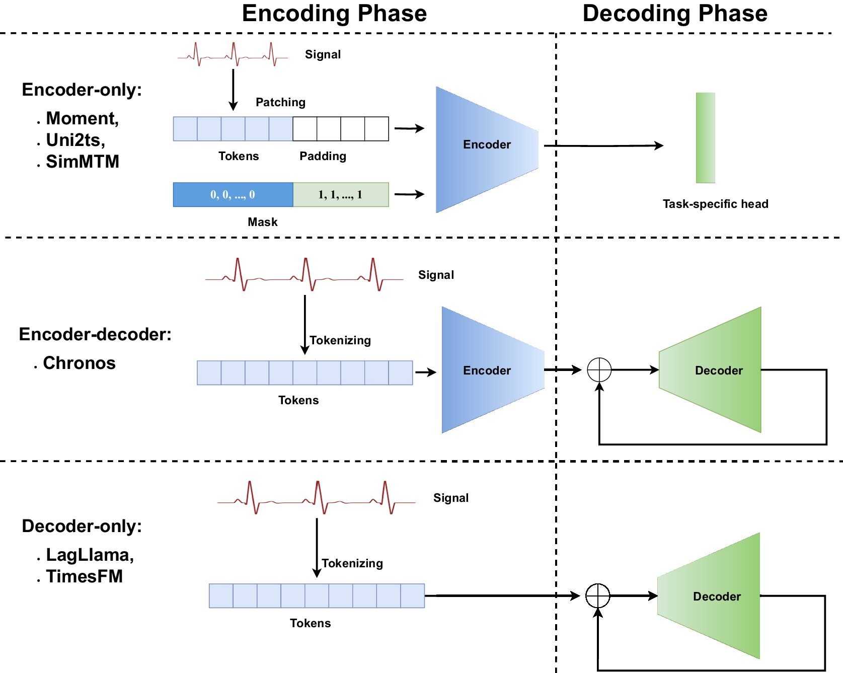
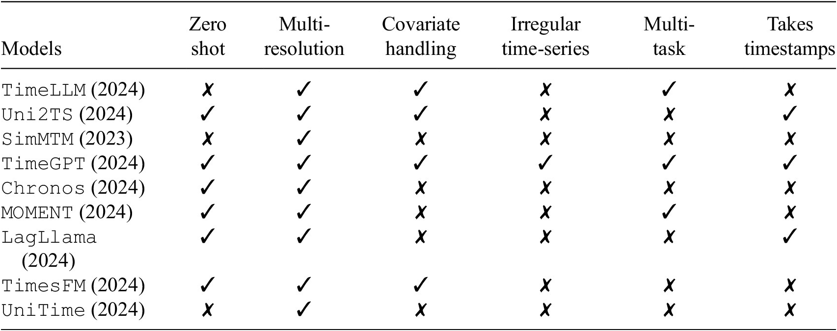
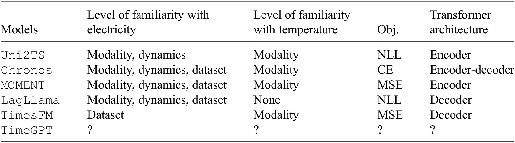

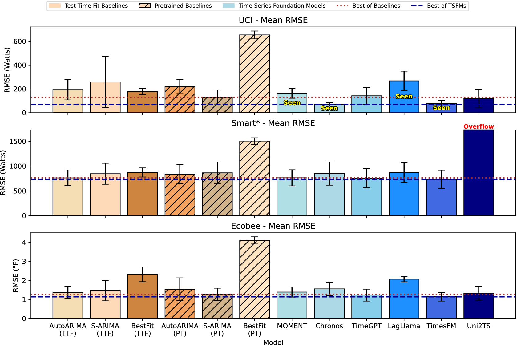


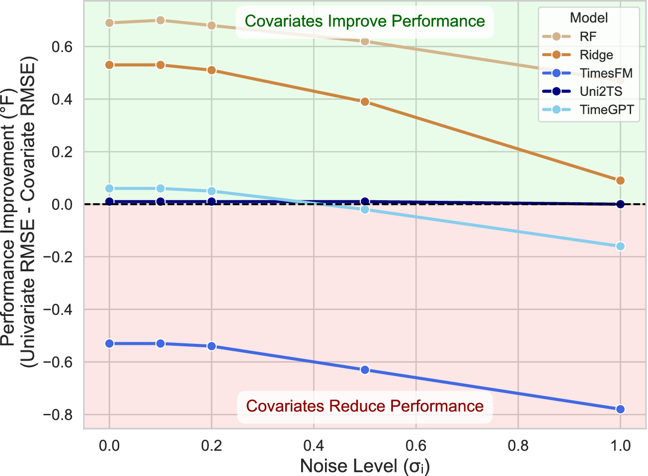


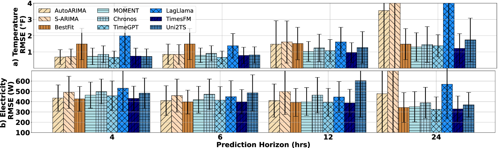


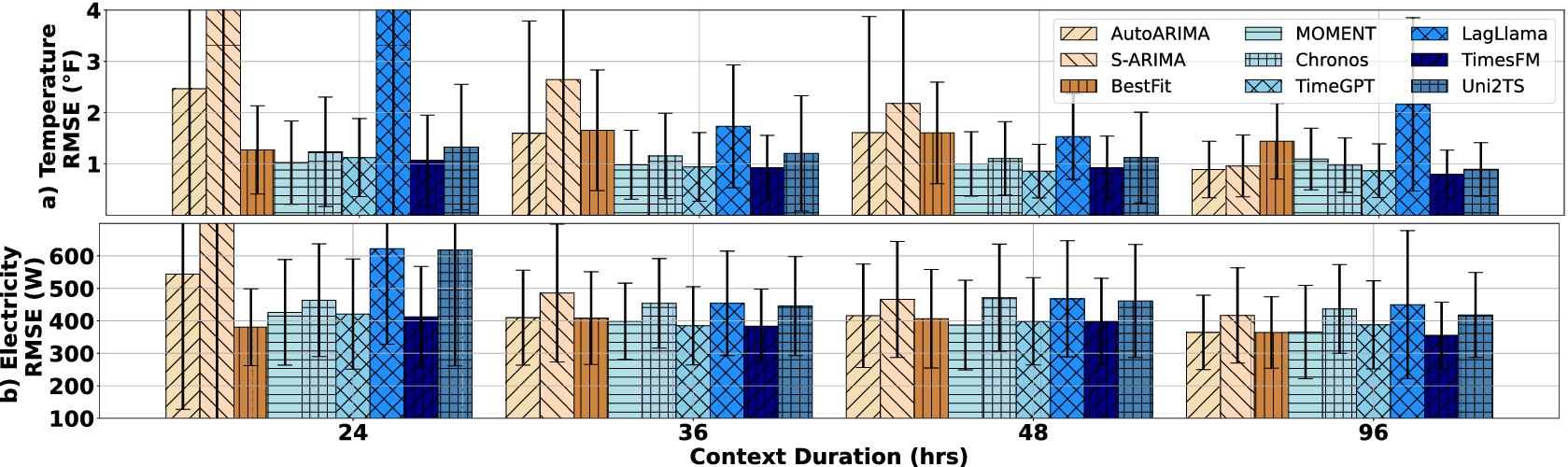


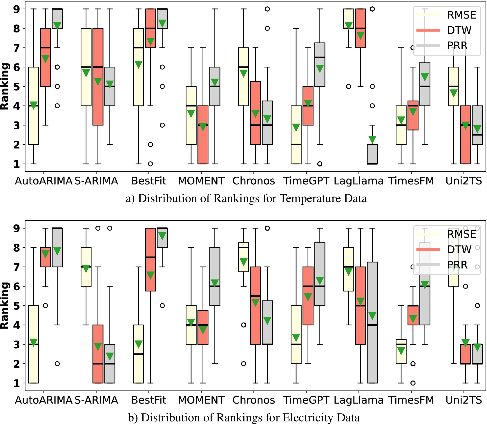


 Open access
Comments
No Comments have been published for this article.