2.1.1 The Major Components of the Climate System

The Earth’s climate system is made up of several major components that are complex and interacting.Footnote ⁷ Together, they govern the Earth’s climate patterns and conditions, changing over time.

The atmosphere is a protective layer of gases that surround the Earth’s surface, which provides the air we breathe, regulates heat to keep the planet warm, and shields us from harmful UV radiation from the sun. The sun’s heat and the Earth’s rotation create movement in the atmosphere; these circulation patterns redistribute heat and moisture across the planet, influencing weather and climate.

The biosphere comprises all living organisms on Earth. It interacts with other climate components through processes like photosynthesis, respiration, and the carbon and nitrogen cycles, which can affect climate through altering greenhouse gas concentrations and the land surface. Together with the ocean, the land absorbs over half of the carbon dioxide emissions emitted by human activities.

The hydrosphere includes the liquid surface and subterranean water, such as in oceans, seas, rivers, freshwater lakes, underground water, wetlands, etc. Covering 70 per cent of the world’s surface, the ocean has a huge capacity to absorb and hold heat, energy, and carbon dioxide. The ocean stores and transfers heat across the globe through its ocean currents and deepwater circulations, which in turn affects climate and weather patterns.

The cryosphere consists of the frozen parts of the Earth such as glaciers, sea ice, ice sheets, and snow. Cryospheric changes can affect other climate components through processes like glacier and ice-sheet melt (impacting sea levels and ocean circulation) or through snow cover melt (impacting the Earth’s energy budget by modifying its albedo – the amount of the sunlight reflected off the Earth’s surface).

Finally, the lithosphere is the upper layer of the solid Earth (continental and oceanic). It can influence the climate through changes in albedo (how much heat a surface absorbs), through the effects of landforms on atmospheric circulation, and through the weathering of rocks that can affect greenhouse gases concentrations such as carbon dioxide.

The climate system is constantly changing with its components interacting with each other. Many other processes – both inside and outside the Earth – affect the climate system, and these are covered later in this chapter.

2.1.2 Different Types of Scientific Evidence

Scientific understanding of the climate system’s features is robust and well established, based on multiple lines of scientific evidence. For centuries, scientists have been measuring and monitoring aspects of the climate system in order to understand how it works, what drives its changes, and to predict future weather. Weather observations of temperature and pressure have been made since the seventeenth century and the first published study that argued carbon dioxide could raise the Earth’s temperature was published in the nineteenth century.Footnote ⁸ Observed evidence for carbon dioxide raising global temperatures was first reported in the early twentieth century.Footnote ⁹ The use of weather and climate observational evidence has steadily grown throughout the centuries. By the twentieth century, systematic and wide-ranging measurements were being made, particularly from the 1970s when satellite-based observations were established, offering near global coverage for many climate variables.

This observational evidence offers a powerful understanding of our climate – however, it is just one line of evidence that scientists use to understand the climate system. Using paleoclimate evidence,Footnote ¹⁰ scientists have reconstructed the Earth’s past climate, dating back hundreds of millions of years into the past. For example, the frozen bubbles taken from ice cores hold information on past temperatures and atmospheric gas concentrations from hundreds of thousands of years ago. Similarly, marine sediment from rock cores can provide information on past temperature, ice volume, and sea level over millions of years. As well as giving relative comparisons for today’s climate changes, these data tell us that the Earth in the past has experienced prolonged periods of elevated greenhouse gas concentrations that caused global temperatures and sea levels to rise. Studying past climate can therefore help us understand future consequences of increasing greenhouse gases in the atmosphere.

A third line of evidence comes from climate models, which are essential tools for scientists to simulate the Earth’s complex climate system. Climate models are computer programs that simulate the Earth’s climate, based on fundamental laws of physics, chemistry, and biology of the atmosphere, ocean, ice, and land. Some models include more processes, complexity, and detail than others, giving them different strengths and weaknesses, but their results can be tested by comparing them with past observations and paleo evidence. Climate models can be used to identify what has caused these past changes, and also to explore how the climate could change in the future under scenarios (see Section 2.4). Climate model complexity and the methods for projecting future changes have matured over the decades, but the IPCC concluded that the projections from even the early, simple climate models quite accurately projected what was subsequently observed.

Finally, scientific understanding of physical, chemical, biological, and geological processes that underpin how the climate works complement evidence from observations, paleoclimatology, and modelling. Ocean and atmospheric circulation, ice-sheet dynamics, radiative forcing (how substances alter the balance of energy entering and leaving the Earth’s atmosphere), cycles such as the carbon or nitrogen cycles, and climate feedbacks (processes that lead to an amplification or a dampening of further climate changes) are all examples of climate processes.

Used together, these multiple lines of evidence provide the backbone of the scientific understanding of climate change. They enable scientists to test hypotheses, attribute the causes of climate change, and inform adaptation and mitigation decision making.Footnote ¹¹ Other sources of knowledge, including Indigenous knowledge, can also provide important insight into climate change and its drivers, impacts, and possible responses.Footnote ¹²

2.1.3 Natural Variability of the Climate

Today, the climate is warming almost everywhere across the globe. While global surface temperature has varied over millennia, the reason for recent warming is different.

Constructed using the lines of evidence described earlier, Figure 2.1 shows how atmospheric carbon dioxide levels (upper panel) and global surface temperature (lower panel) have varied over the past 60 million years and how they could evolve into the future, to the year 2300. Temperature changes are all relative to a baseline period just before the industrial revolution (1850–1900). There has always been a close relationship between carbon dioxide and global temperature but the causes of these changes that are happening now are very different compared to the changes that have occurred in the past.

Figure 2.1 Historical records of global carbon dioxide concentration levels (parts per million, ppm) and temperature (°C) over the past 60 million years. For context, humans developed around 250,000 years ago, and agriculture only developed 10,000 years ago with a more stable and warmer climate.Footnote ¹³

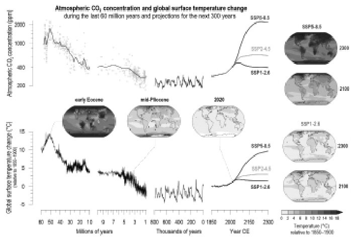
Natural causes of climate change refer to variations in climate that can be either externally driven by natural changes or internally generated within the climate system. Figure 2.1 shows how some external natural variability can operate on very long time scales (see the 800,000–0 years axis in Figure 2.1). These temperature and carbon dioxide changes result from changes in the Earth’s orbit around the sun. These orbital changes alter the amount of energy absorbed by the Earth from the sun and operate over (very long) time scales of tens-to-hundreds of thousands of years.Footnote ¹⁴ These orbital shifts alone are not enough to explain the large changes in temperature seen in the past ice ages – global average temperature then was around 4°C cooler than it is today – but they kick-start other processes that further amplify the changes to temperature and carbon dioxide levels. More ice on the Earth’s surface causes more of the sun’s energy to be reflected back to space, therefore further cooling the Earth. This is one example of what is referred to as climate feedback. More ice in colder temperatures also means lower sea levels, which results in more land area and more growing vegetation that absorb carbon dioxide, thus lowering atmospheric levels. Volcanic eruptions are another example of external natural variability, as volcanoes are not part of the climate system but can still cause changes. Large volcanic eruptions can cool the Earth through the particles that they emit, acting as a shield to the sun’s rays and reflecting back some incoming radiation. This effect is short-lived: the effect on surface temperature typically fades within a decade after the eruption.

Much like the effects of volcanic eruptions, effects of internal natural variability also span over shorter time frames of years to decades. Internal natural variability refers to when energy within the climate system redistributes among the different climate components (atmosphere, hydrosphere, etc.). These changes are more clearly observed regionally compared to on the global scale. One example of internal natural variability is El Niño–Southern Oscillation (ENSO), a climate pattern in the tropical Pacific that oscillates between two phases over a period of two to seven years. The ENSO phase influences a variety of weather phenomena around the world, intensifying heat extremes during the El Niño phase, for example.

Natural variability causes major year-to-year or even decadal changes in global surface climate, but over the longer term, it plays a smaller role. Over multiple decades or longer, the oscillations caused by natural variability are clearly discernible from long-term trends caused by human influence. When combined with human-caused climate changes, the consequences of natural variability can be either larger or smaller than initially projected. For those regions affected by ENSO, for example, the human-caused changes to rainfall and wildfires can be a bit larger, or smaller, for that short period of time. There is always a chance that future changes could be a bit stronger (or a bit weaker) than projected – but these natural factors will have little effect on long-term trends.Footnote ¹⁵

By comparing today’s temperature and carbon dioxide levels with past changes to the climate, it is clear that the recent warming is different from before. Carbon dioxide levels are already their highest in at least two million years. Global temperatures are their highest in at least 100,000 years. The speed of warming over the last 50 years was faster than any other 50-year period over the past 2,000 years. Recent warming reverses a long-term global cooling trend. After the last ice age, global surface temperature peaked around 6,500 years ago, then started to slowly decline. It was not until the mid nineteenth century that the long-term cooling trend started to reverse with now persistent and prominent warming. Today the climate is warming almost everywhere across the globe. Over the past 2,000 years, some regions have always experienced periods of more or less warming than the global average. For example, the North Atlantic region warmed more than many other regions during the tenth and thirteenth centuries, but almost every region of the world is now experiencing sustained warming since the industrial revolution.Footnote ¹⁶

The right-hand side of Figure 2.1 shows how global temperatures and carbon dioxide levels could evolve in the coming centuries depending on the choices made by society. Some projected global temperature changes would be larger than the Earth has experienced for over three million years. This is discussed further in Section 2.4.1.

2.1.4 The Greenhouse Effect

The Earth’s energy budget describes the flow of energy within the climate system. Our planet receives vast amounts of energy every day in the form of sunlight. Around a third of the sunlight is reflected back to space by clouds, by tiny particles called aerosols, and by bright surfaces such as snow and ice. The rest is absorbed by the ocean, land, ice, and atmosphere. The planet then emits energy back out to space in the form of thermal radiation. In a world that was not warming or cooling, these energy flows would balance. Some gases in the atmosphere – such as carbon dioxide, methane, and nitrous oxide – warm the Earth by absorbing and then re-radiating some of the energy emitted by the planet as heat. These gases make it harder for heat to be released into outer space. Instead, it is transferred into the climate system.Footnote ¹⁷

This effect is called the greenhouse effect, as the same mechanism occurs in a greenhouse, with walls of the greenhouse trapping warmer air inside, making it warmer than its surroundings. Facilitated by greenhouse gases occurring naturally in the atmosphere, the greenhouse effect is a natural process that makes the Earth liveable for humans: without the natural greenhouse effect, the global average temperature would be about 33ºC (59°F) colder. However, human activities since the industrial revolution have led to additional, anthropogenic greenhouse gases accumulating in the atmosphere. These emissions result mostly from burning fossil fuels (coal, oil, and gas) but also from agriculture and cutting down forests. These actions have boosted the greenhouse effect, causing global warming and disruption of the climate system. The excess energy is taken up by different parts of the Earth: 91 per cent is absorbed by the oceans, 5 per cent is absorbed by the land, 3 per cent is absorbed by the ice. Only 1 per cent of the extra heat is absorbed by the atmosphere. Although the mechanism of the greenhouse effect is relatively simple, the causal mechanisms through which this imbalance in energy manifests itself throughout the climate system, and how these modifications impact societies and ecosystems across the globe, are more complex. The remainder of this chapter will delve into these complexities and unpack a wealth of scientific evidence demonstrating that the impacts of a changing climate have been and will continue to be profound and widespread.Footnote ¹⁸

2.2.1 Greenhouse Gas Emissions Sources and Trends

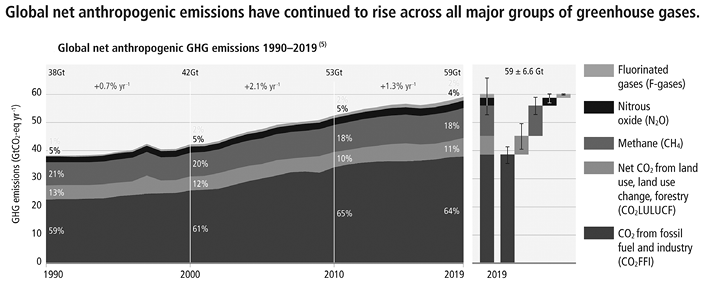
Since 1850, emissions of greenhouse gases into the atmosphere have steadily increased, totalling 2,400 ± 240 GtCO₂Footnote ¹⁹ until the year 2019. Despite the growth rate slowing in the 2010–2019 decade, the average greenhouse gas emissions over this decade were higher than any other previously recorded. Figure 2.2 shows how the net emissions of the major anthropogenic greenhouse gases have changed for the years 1990–2019. The largest amount of net emissions are of carbon dioxide. Emission totals for the year 2019 were calculated to be 59 ± 6.6 GtCO₂–eq,Footnote ²⁰ which is 12 per cent higher than 2010 levels and 54 per cent higher than 1990 levels. The largest share and growth in greenhouse gas emissions comes from carbon dioxide emissions resulting from fossil fuels combustion and industrial processes (64% of 2019 emissions), followed by methane (18% of 2019 emissions). Of the 2019 emission total, 11 per cent was carbon dioxide emissions associated with land use and land-use change (e.g. deforestation).Footnote ²¹

Figure 2.2 Global net anthropogenic GHG emissions (GtCO₂–eq yr^–1) 1990–2019. Global net anthropogenic GHG emissions include CO₂ from fossil fuel combustion and industrial processes (CO₂–FFI); net CO₂ from land use, land-use change, and forestry (CO₂–LULUCF); methane (CH₄); nitrous oxide (N₂O); and fluorinated gases (HFCs, PFCs, SF₆, NF₃). At the right side of the panel, associated uncertainties for each of the components for 2019 are shown.Footnote ²²

Both historically and at present, the regional distribution of emissions across the globe has been very unequal. Figure 2.3 shows the historical contribution (1850–2019) of carbon dioxide per region. Fossil fuel and industry and land use, land-use change, and forestry emissions are shown in panel (a). North America has contributed the highest share of historical carbon dioxide emissions (23%) followed by Europe (16%) and East Asia (12%). Panel (b) compliments the historical contributions by showing the 2019 contributions, including other major greenhouse gases, and is weighted by population across the regions, showing the per capita distributions. Taller, narrower rectangles represent regions with lower populations but larger emissions. North America still remains the region with the highest contribution to emissions on a per capita and total population basis.Footnote ²³

Figure 2.3 Regional differentiations of greenhouse gas emissions. Panel (a): Cumulative regional carbon dioxide emissions from 1850 to 2019. Panel (b): Regional GHG emissions in tonnes CO₂–eq per capita by region in 2019. Note that emissions from international aviation and shipping are not included. Key: Black = CO₂ from fossil fuel combustion and industrial processes (CO₂–FFI); Dark grey = net CO₂ from land use, land-use change, and forestry (CO₂–LULUCF); Light grey = Other GHG emissions.Footnote ²⁶

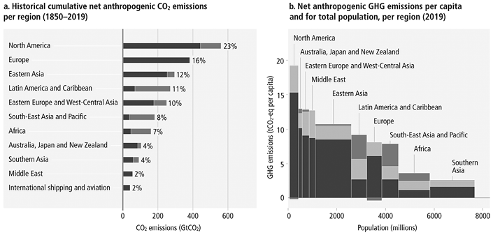
The global average emissions per person is 6.9 tCO₂–eq for the year 2019 (not including land-use-related emissions). Around 35 per cent of the global population live in countries emitting more than 9 tCO₂–eq per capita while 41 per cent live in countries emitting less than 3 tCO₂–eq per capita, and, of the latter, a substantial share lacks access to modern energy services. LDCs and SIDS have much lower per capita emissions than the global average (1.7 tCO₂–eq and 4.6 tCO₂–eq, respectively).Footnote ²⁴

Globally, the 10 per cent of households with the highest per capita emissions contribute 34–45 per cent of consumption-based household greenhouse gas emissions, while the bottom 50 per cent contribute 13–15 per cent.Footnote ²⁵

In 2015, countries adopted the Paris Agreement, which set a goal of holding ‘the increase in the global average temperature to well below 2°C above pre-industrial levels’ and pursuing efforts ‘to limit the temperature increase to 1.5°C above pre-industrial levels’.Footnote ²⁷ In order to achieve this long-temperature goal, immediate and drastic reductions of greenhouse gas emissions are needed. Regional contributions to these reductions should reflect the principles of ‘equity’ and ‘common but differentiated responsibilities and respective capabilities’, to enable a just transition.Footnote ²⁸ In contrast to previous reports, the IPCC’s Sixth Assessment Report does not provide quantitative indications of how these regional differences could be reflected in mitigation targets. The onus is therefore on other mechanisms and actors to specify equity principles and quantify their implications. National and regional courts are increasingly being asked to determine questions relating to climate change and equity, including if the climate actions pledged by States are adequate in relation to their fair share of what is globally required, as it is only in relation to such a ‘fair share’ that the adequacy of a State’s contribution can be assessed in the context of a global collective action problem.Footnote ²⁹

2.2.2 Attributing Human Influence on the Climate

Using the multiple lines of evidence described in this chapter’s introduction (Section 2.1), the level of human influence on global warming and many other aspects of changes in the climate system are now known. Attributing the causes of climate change largely refers to three main concepts: the attribution of observed climate change to human influence, the attribution of weather and climate extreme events to human influence, and the attribution of impacts on ecosystems and human systems to changing climate and to human influence. This section provides an overview of the current evidence using attribution methods.Footnote ³⁰ The following chapter on attribution science dives deeper into this topic.

2.2.2.1 Attribution of Human Influence to Observed Climate Change

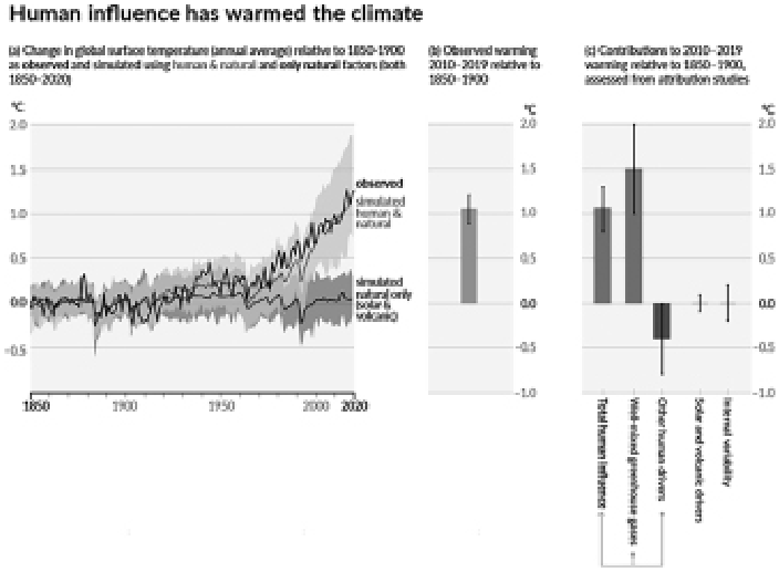
Since 1850–1900, human activities have unequivocally caused global warming, with global surface temperature reaching 1.1°C (2°F) in the decade 2011–2020 (1.09 [0.95 to 1.20]°C). All of the observed global surface temperature increase can be attributed to human activities, as Figure 2.4 shows. This figure uses evidence from ‘fingerprint’ attribution studies, which synthesise and compare information from climate models and observations. Panel (a) compares observations with climate simulations that take into account only natural drivers or natural and human drivers. It is only when climate model simulations include human-caused greenhouse gases that they can recreate temperature observations. By comparing the total observed warming (panel (b)) with the warming amount from different contributors (panel (c)), it can be seen that greenhouse gas emissions from human activities would have in fact warmed the Earth even more than what has been observed, by about 1.5ºC (2.7°F) in total. Their total warming effect has been partly counteracted by emissions of air pollutants called aerosols, which have an overall cooling effect. Carbon dioxide is the greenhouse gas that contributes the most to the warming (~0.8°C), followed by methane (~0.5°C), nitrous oxide (~0.1°C), and fluorinated gases (~0.1°C). Solar and volcanic drivers of the climate changed temperatures by –0.1°C to 0.1°C, and internal variability changed it by –0.2°C to 0.2°C.Footnote ³¹

Figure 2.4 Observed warming is caused by emissions from human activities, with greenhouse gas warming partly masked by aerosol cooling. Panel (a): Changes in global surface temperature over the past 170 years (thick black line) relative to 1850–1900 and annually averaged, compared to climate model simulations (CMIP6) of the temperature response to both human and natural drivers (dark grey line and shading), and to only natural drivers (solar and volcanic activity) (light grey line and shading). Solid lines show the multi-model average, and shading shows the very likely range of simulations. Panel (b): The bar shows the observed increase of global surface temperature in 2010–2019 relative to 1850–1900 and its uncertainty range (black error bar line). Panel (c): Temperature change in 2010–2019 relative to 1850–1900 attributed to total human influence, change in well-mixed greenhouse gases concentrations, other human drivers (aerosols, ozone, and land-use change), natural drivers (solar and volcanic), and internal climate variability. Whiskers show uncertainty ranges (black error bar lines).Footnote ³²

Human influence on multiple other changes occurring in the climate system has also been attributed. The IPCC assessment attributes human influence as the ‘main driver’ (contributing more than 50 per cent) of, or as a contributor to, the following changes. The level that human influence is attributable as the main driver is expressed using a likelihood phrasing that has a probabilistic definition or a qualitative phrasing of confidence. Note that if no confidence or likelihood term is stated in the list then the change has only been observed and not fully attributed. Confidence and likelihood terms are defined using the IPCC guidelines.Footnote ³³

• The global retreat of glaciers (very likely main driver of, since the 1990s).

• The decrease in Arctic sea-ice area (very likely main driver of, since the late twentieth century).

• Decreased northern hemisphere spring snow cover (very likely main driver of, since 1950).

• The surface melting of the Greenland Ice Sheet (very likely main driver of, over the past two decades).

• Global mean sea level rise (very likely main driver of, at least since the 1970s), the rate of which has since been accelerating, as ice-sheet and glacier mass loss are now the dominant contributors to rising global mean sea level.

• The warming of the global upper ocean (extremely likely main driver of, since the 1970s).

• Global acidification of the surface open ocean (virtually certain main driver of).

• Reduced oxygen levels in many upper ocean regions (medium confidence contributed to, since the mid twentieth century).

• Changes in near-surface ocean salinity (extremely likely contributed to).

• Increased globally averaged precipitation over land (likely contributed to, since 1950), with a faster rate of increase since the 1980s.

• The shift of mid-latitude storm tracks polewards in both hemispheres (since the 1980s).

• The poleward shift of the southern hemisphere extratropical jet in austral summer (very likely contributed to, since the 1980s).

• A shift polewards of climate biosphere zones in both hemispheres (since the 1970s), and the growing season has on average lengthened in the Northern Hemisphere extratropics (since the 1950s).

2.2.2.2 Attribution of Weather and Climate Extreme Events to Human Influence

It is also now possible to attribute the change in likelihood or characteristics of specific regional weather or climate events or classes of events to underlying drivers, including human influence. Extreme events where an attributable human influence have been identified include hot and cold temperature extremes (including some with widespread impacts), heavy precipitation events, certain types of droughts, and tropical cyclones.Footnote ³⁴

Human-induced climate change is already affecting many weather and climate extremes. In previous IPCC reports, it was not possible to say if or how much human-caused climate change contributed to individual extreme events, but this is now possible with the development of new scientific methods. For most of these extremes, the extent to which human influence is the main driver of or has contributed to these climate changes can be described using a likelihood or confidence phrasing.Footnote ³⁵

• Hot extremes have become more frequent and more intense across most land regions (high confidence main driver of, since the 1950s). The occurrence of some hot extremes would have been extremely unlikely to occur without human influence over the past decade. On a global scale, hot extreme events that used to have a one-in-fifty-year likelihood during the pre-industrial period have now become approximately five times more probable due to human activities. Similarly, events with a one-in-ten-year probability have become almost three times more likely.

• Cold extremes have become less frequent and less severe (high confidence main driver of, since the 1950s).

• Increased marine heatwaves (very likely contributed to, since at least 2006). Marine heatwaves have approximately doubled in frequency since the 1980s.

• Increased frequency and intensity of heavy precipitation over land where data allows for analysis (likely contributed to, since the 1950s).

• Increased agricultural and ecological droughts in some regions due to increased land evapotranspiration (medium confidence contributed to, since the 1950s).

• Increased occurrences of the major (Category 3–5) tropical cyclones (since the 1970s).

• Although there has been no overall increase in the annual number of tropical cyclones, they are now likely stronger (the proportion of Category 3–5 tropical cyclones has increased since the 1970s) and this cannot be explained by only natural variability.

• Increased heavy precipitation associated with tropical cyclones (supported by attribution studies and physical process understanding but not observed on the global scale due to data limitations).

• Increased chance of compound extreme events (since the 1950s). Compound extreme events are the combination of multiple drivers and/or hazards that contribute to societal or environmental risk and include concurrent heatwaves and droughts, fire weather in some regions of all inhabited continents, and compound flooding.

• Human activities have impacted the global monsoon system, although in this case there is a complex interplay between the influence of climate-warming greenhouse gases and other types of air pollution.

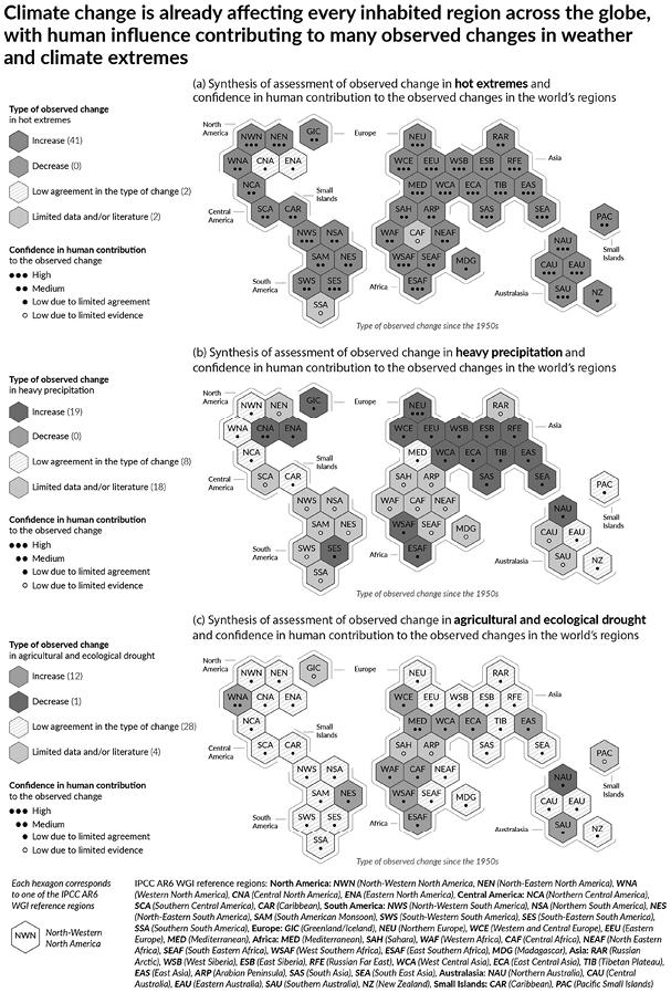
Figure 2.5 is a synthesis of assessed observed and attributable regional changes. It shows that human-caused climate change has already affected all inhabited regions around the world through occurrences of hot extremes, heavy precipitation events, and agricultural and ecological droughts. When the IPCC was first established, it was not possible to confirm that climate change was already happening, but now we are able to actually observe and attribute changes all across the world of human-caused climate change.

Figure 2.5 Synthesis of assessed observed and attributable regional changes for (a) hot extremes (b) heavy precipitation and (c) agricultural and ecological drought. The inhabited regions as defined in the IPCC Working Group I Sixth Assessment Report are displayed as hexagons with identical size in their approximate geographical location. The shading of each hexagon corresponds to observed changes. The dots within each hexagon indicate the level of confidence in the human contribution to these changes. All assessments are made for the 1950s to the present. White and light-grey striped hexagons are used where there is low agreement in the type of change for the region as a whole, and light grey hexagons are used when there is limited data and/or literature that prevents an assessment of the region as a whole.Footnote ³⁶

2.3.1 Widespread, Unprecedented Climate Changes

The influence of human activities is propelling the Earth’s climate into uncharted territory. Many of the climate changes being felt across the globe are unprecedented in over hundreds, if not thousands, or even millions, of years. Continued increases in atmospheric greenhouse gas concentrations reached annual averages of 410 parts per million (ppm) for carbon dioxide, 1,866 parts per billion (ppb) for methane, and 332 ppb for nitrous oxide in 2019. These levels were higher than any time in at least two million years for carbon dioxide and 800,000 years for methane and nitrous oxide. Global surface temperatures have increased faster since 1970 than in any other 50-year period over at least the last 2,000 years. Each of the last four decades has been warmer than any previous decade since 1850 and the years 2011–2020 were the warmest decade the world has experienced in at least the last 100,000 years. The area of the Arctic Ocean covered by sea ice in the summer is now 40 per cent smaller than in the 1980s. It is the smallest it has been for at least 1,000 years. The near global retreat of all glaciers since the 1950s is unprecedented in at least the last 2,000 years. By absorbing carbon dioxide from the atmosphere, the ocean is becoming more acidic. The surface water of the ocean is now unusually acidic compared with the last two million years. Global mean sea level has risen ~0.20m between 1901 and 2018. This increase was faster than in any preceding century over the last 3,000 years. The global ocean has warmed faster in the past century than during the end of the last deglacial transition around 11,000 years ago.Footnote ³⁷

2.3.2 Resulting Impacts on Ecosystems and Societies

Human-induced climate change, including more frequent and intense extreme events, has caused widespread adverse impacts and related losses and damages to nature and people, beyond natural climate variability (Figure 2.6). They manifest as the consequence of a spectrum of climatic events, ranging from the sudden intensity of extreme occurrences like heatwaves, floods, storm surges, hurricanes, and cyclones to the gradual onset of phenomena such as increasing temperatures, glacial retreat, prolonged droughts, ocean acidification, and rising sea levels. Impacts on terrestrial, freshwater, and ocean ecosystems include species losses and changes in timing such as flowering and growing seasons.

Figure 2.6 Observed global and regional impacts on (a) ecosystems and (b) human systems attributed to climate change at global and regional scales. Confidence levels in the attribution of the observed impacts to climate change are given. Global assessments focus on large studies, multi-species, meta-analyses, and large reviews. For that reason, they can often be assessed with higher confidence than regional studies, which often rely on smaller studies that have more limited data. Regional assessments consider evidence on impacts across an entire region. For human systems (b), the + and – symbols indicate the direction of observed impacts, with a – denoting an increasing adverse impact and a ± denoting that, within a region or globally, both adverse and positive impacts have been observed.Footnote ³⁸

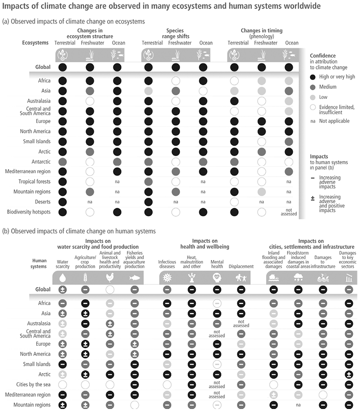
Climate change has resulted in a wide array of detrimental impacts on human systems, spanning from water security and food production to health and overall well-being, as well as impacts on urban areas, communities, infrastructure, and economies. The most vulnerable countries and communities, which historically are those that have contributed the least to current climate change, are disproportionately impacted with devastating consequences on their lives and livelihoods. Some examples of impacts, detailed in the IPCC WGII report, are given later.

2.4.1 Climate Scenarios and Future Global Temperatures

The climate we and the young generations will experience depends on future emissions. Reducing emissions rapidly will limit further changes, but continued emissions will trigger larger changes that will increasingly affect all regions. Many changes will persist for hundreds or thousands of years, so today’s choices will have long-lasting consequences.

To study how climate change can evolve into the future, the scientific community often uses scenarios. The IPCC defines scenarios as ‘plausible description[s] of how the future may develop based on a coherent and internally consistent set of assumptions about key driving forces and relationships’. In addition, the IPCC notes that scenarios ‘are neither predictions nor forecasts, but are used to provide a view of the implications of developments and actions’.Footnote ⁴⁴ The driving forces in the IPCC’s definition of scenarios can refer to assumptions about economic and population growth, inequality, technological innovation and costs, or dietary or other societal preferences, amongst many other things.Footnote ⁴⁵ The relationships referred to in the definition indicate that not any combination of assumptions is possible. For example, it is highly unlikely that an unequal world with low educational attainment or low levels of female education would see the highest rates of technological innovation.

Climate change scenarios are created and assessed by different types of scientific models. A first type of model known as Integrated Assessment Models (IAMs) creates emissions scenarios. Emissions scenarios describe how society can meet its future energy, food, and other demands while limiting climate change, and report the implied resulting greenhouse gas emissions. These emissions scenarios are subsequently used by a different type of model, typically referred as climate models, to estimate how these emissions would affect future climate change. These climate models report how temperature, precipitation, or humidity might change in the future, when a specific emissions scenario is followed. Socioeconomic or ecological impacts are then explored by a last type of model, known as impact models. Using climate change scenario information from IAMs and climate models, these specialised models estimate the climate change impact of an emissions scenario for a specific sector or system, be it agriculture, flood risks, human health, and many more.

Because the range of possible futures is large, the scientific community has developed a framework to explore scenarios in a more systematic way. This is known as the framework of the Shared Socioeconomic Pathways or SSPs. The SSPs describe five distinct future socioeconomic contexts (SSP1 to SSP5) that differ between them in the degree to which mitigation and adaptation efforts experience challenges. For example, SSP1, called Sustainability, sketches a future socioeconomic context with reducing inequalities, increasing international collaboration and innovation, and a switch to healthy and environmentally conscious lifestyles. In an SSP1 world, implementing adaptation and mitigation measures is considered to encounter only low challenges. On the contrary, SSP3, called Regional Rivalry, describes a world with resurgent nationalism, exacerbating inequalities both within and between countries, and consequently low levels of technological innovation. Such an SSP3 world reflects a context with high challenges to effectively implement adaptation and mitigation measures. Other SSPs describe other socioeconomic futures with SSP2 covering a middle-of-the-road scenario that continues historical dynamics. For each of these SSP futures, the scientific community then explores how low global warming can be kept or what the implications of global warming are for adaptation and impacts.Footnote ⁴⁶ Despite their usefulness, the SSPs do not exhaustively cover the space of future socioeconomic possibilities. Both the scientific literature and the IPCC therefore make use of scenarios that are entirely independent of the SSPs, for example, exploring strong improvements in energy efficiency and reducing energy demand.Footnote ⁴⁷

The IPCC also makes use of scenarios to integrate insights across chapters and reports. For example, the Physical Science report (Working Group I) of the IPCC Sixth Assessment uses a selection of five emissions scenarios, discussed later on (see also Figure 2.7). These span a range from very high to very low future greenhouse gas emissions and allow climate change projections from climate models to be easily compared and assessed. In contrast, the Mitigation report (Working Group III) of the IPCC Sixth Assessment is tasked with the assessment of the entire climate scenario literature. They therefore take a different approach. On the one hand, they collect as many emissions scenarios as possible from the published literature in a centralised database that underpins the broader IPCC assessment.Footnote ⁴⁸ The large set of emissions scenarios that is included in this database helps to explore the many potential strategies that can be pursued for limiting global warming to a specific level. To showcase this variety even more clearly, the IPCC also selected a small set of seven ‘illustrative mitigation pathways’ which illustrate the diverse strategies that can be followed while reducing greenhouse gas emissions. Finally, IPCC scenario databases are also made freely available online for further use and analysis by others.Footnote ⁴⁹

Figure 2.7 Linking carbon dioxide emissions, global warming, and effects on the climate systems. Panel (a): Top – Annual emissions of carbon dioxide for the five core Shared Socioeconomic Pathway (SSP) scenarios (very low: SSP1–1.9, low: SSP1–2.6, medium: SSP2–4.5, high: SSP3–7.0, very high SSP5–8.5). These scenarios are illustrative, meaning that they are not intended to be predictions of what will happen in the future; instead they serve an informative purpose to see how the Earth will respond to different situations. Bottom – Projected warming for each of these emissions scenarios. This figure is sourced from the Technical Summary Infographic. Panel (b): Top – How temperature extremes, droughts, heavy rainfall (precipitation) events, snow cover, and tropical cyclones change at different levels of global warming compared with the late nineteenth century (1850–1900). Today, here is the average over 2011–2020. Bottom – Long term (2,000 and 10,000 years) committed sea level rise for global warming of 1.5°C, 2°C, and 4°C).Footnote ⁵²

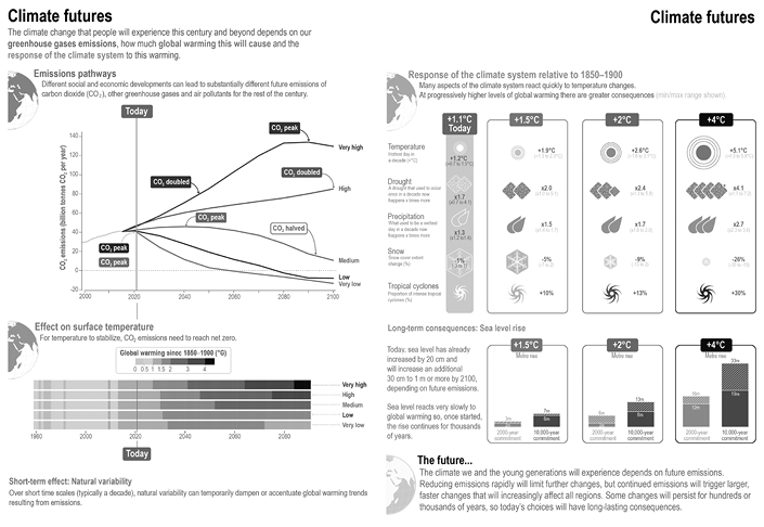
Five scenarios showing how carbon dioxide emissions could change in the future are shown in Figure 2.7. These scenarios are based on the five core SSP scenarios referred to earlier. The lower part of Figure 2.7 (panel (a)) depicts the projected warming for each of these emissions scenarios. It shows that global warming continues to rise until at least around 2050 in all of the five scenarios. This is because the human activities that cause greenhouse gas emissions cannot stop immediately. Even with ambitious action, it will take time to implement actions to reduce greenhouse gas emissions, resulting in a continued increase in temperatures before stabilising. Nevertheless, strong reductions in greenhouse gases starting now would slow and reduce the total amount of warming. Projected temperatures look very different after the 2050s, depending on the actions we take now and in the near future. For example, if carbon dioxide emissions are strongly and rapidly reduced starting now and throughout the twenty-first century, warming would be halted by around the middle of the century, reaching around 1.5°C (2.7°F) or 2°C (3.6°F) by the end of the century. On the other hand, if emissions remain the same or increase, temperatures will continue to rise. In scenarios that look at very high levels of greenhouse gas emissions, warming reaches around 4.5°C (8°F) by the end of the century.

These climate scenarios show that the world will most likely reach 1.5°C (2.7°F) global warming within the period 2021–2040.Footnote ⁵⁰ Unless there are rapid, strong, and sustained reductions in greenhouse gas emissions, limiting warming to 1.5°C (2.7°F) or even 2°C (3.6°F) will be impossible.Footnote ⁵¹ The following section assesses the projected warming associated with countries’ current NDCs and climate policies.

2.4.2 Fast and Slow Onset Climate Changes

Looking ahead, many aspects of climate change will continue to increase or intensify as the Earth becomes warmer. Extremes such as heatwaves, heavy rainfall, and droughts will continue to become more severe and more frequent. Rising temperatures and worsening extreme events are examples of so-called climate change ‘fast’ responses because they react relatively quickly to rising atmospheric greenhouse gas concentrations. All of these examples respond roughly linearly to rising carbon emissions, meaning that every increment of global warming leads to noticeable and discernible changes and impacts on ecosystems and society. An extreme heatwave that used to happen once in every ten years in the pre-industrial era is now 2.8 times as likely to occur, and this will become 5.5 times as likely to occur in a 2°C warmer world. Similarly, a heavy precipitation event that used to happen once in every ten years in the pre-industrial era is era is now 1.3 times as likely to occur, and this will become 1.7 times as likely to occur in a 2°C warmer world. Globally, the intensity of precipitation increases ~7 per cent on average for every degree of global warming. An extreme agricultural and ecological drought that used to happen once in every ten years in the pre-industrial era is now 1.7 times as likely to occur, becoming 2.5 times as likely to occur in a 2°C warmer world.Footnote ⁵³

The water cycle will intensify and be more variable although not always linearly due to the complex interaction with pollution aerosols as described earlier in this chapter. Rainfall over land, including monsoon rainfalls, will become more variable and intense: some areas will get drier, others will get wetter. Further warming will also amplify the thawing (defrosting) and melting of many frozen parts of the world, such as snow cover, glaciers, frozen ground, and Arctic sea ice. For instance, it is estimated that the Arctic Ocean will be effectively free of sea ice at its lowest point in summer (September) at least once before 2050. Tropical cyclones will get stronger. The differences in severity of some climate changes at 1.5°C (2.7°F), 2°C (3.6°F), and 4°C (7.2°F) global warming are illustrated in Figure 2.7 (panel (b)).Footnote ⁵⁴

Compound extreme events are the combination of multiple drivers and/or hazards over space and time that contribute to societal or environmental risk. Their probability of occurrence is projected to increase with global warming. They can occur on various spatial scales from sub-national to global and can often impact ecosystems and societies more strongly than when such events occur in isolation. Examples are concurrent heatwaves and droughts in multiple locations, compound flooding (e.g. a storm surge in combination with extreme rainfall and/or river flow), compound fire weather conditions (i.e. a combination of hot, dry, and windy conditions), or concurrent extremes at different locations such as in multiple crop-producing regions. Compound extremes at multiple locations, including in crop-producing areas, become more frequent at 2°C and above compared to 1.5°C global warming.Footnote ⁵⁵

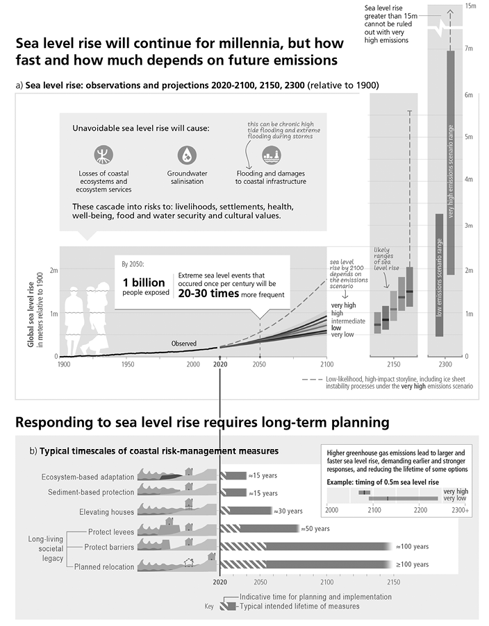
There are many changes that will continue for hundreds or thousands of years as they react very slowly to rising greenhouse gas emissions and a warming world. Changes like deep ocean warming, Greenland and Antarctica ice-sheet melting, carbon lost from thawing permafrost, and sea level rise are slow to respond to the atmosphere warming but will continue to change for centuries, if not millennia. These changes are deemed irreversible because they would continue to change on these time scales even if greenhouse gases or global temperatures were stabilised or brought back down again. The bottom of panel (a) in Figures 2.7 and 2.8 illustrate the long-term committed changes of sea level rise as a result of climate change: even if global warming can be stabilised at 1.5°C (2.7°F), sea level would still rise 2–3 metres (7–10 feet) over the coming 2,000 years and 6–7 metres (20–23 feet) over the coming 10,000 years. Stabilising at higher levels of global warming will result in increased committed changes and will increase the rate of these changes compared to stabilising at global warming levels like 1.5°C (2.7°F).Footnote ⁵⁶ Figure 2.8 shows how these committed sea level changes compare to timelines of implementing various adaptation options.

Figure 2.8 Observed and projected global mean sea level change and its impacts, and time scales of coastal risk management. Panel (a): Global mean sea level change in metres relative to 1900. The historical observed changes (black line) are recorded by tide gauges before 1992 and altimeters afterwards. The future changes from 2020 to 2100 and for 2150 are assessed consistently with observational constraints based on emulation of CMIP, ice-sheet, and glacier models, and median values and likely ranges are shown for the considered scenarios. Relative to 1995–2014, the likely global mean sea level rise by 2050 is between 0.15 to 0.23 m in the very low GHG emissions scenario (SSP1–1.9) and 0.20 to 0.29 m in the very high GHG emissions scenario (SSP5–8.5); by 2100 between 0.28 to 0.55 m under SSP1–1.9 and 0.63 to 1.01 m under SSP5–8.5; and by 2150 between 0.37 to 0.86 m under SSP1–1.9 and 0.98 to 1.88 m under SSP5–8.5 (medium confidence). Changes relative to 1900 are calculated by adding 0.158 m (observed global mean sea level rise from 1900 to 1995–2014) to simulated changes relative to 1995–2014. The future changes to 2300 (bars) are based on literature assessment, representing the 17th–83rd percentile range for SSP1–2.6 (0.3 to 3.1 m) and SSP5–8.5 (1.7 to 6.8 m). Dashed lines are showing a low-likelihood, high-impact storyline including ice-sheet instability processes. These indicate the potential impact of deeply uncertain processes and show the 83rd percentile of SSP5–8.5 projections that include low-likelihood, high-impact processes that cannot be ruled out; because of uncertainty surrounding these processes in the projections, this is not included as part of a likely range. IPCC AR6 global and regional sea level projections are hosted at https://sealevel.nasa.gov/ipcc–ar6–sea–level–projection–tool. The low-lying coastal zone is currently home to around 896 million people (nearly 11% of the 2020 global population), projected to reach more than one billion by 2050 across all five SSPs. Panel (b): Typical time scales for the planning, implementation (dashed white and grey bars), and operational lifetime of current coastal risk-management measures (fully grey bars). Higher rates of sea level rise demand earlier and stronger responses and reduce the lifetime of measures (inset). As the scale and pace of sea level rise accelerates beyond 2050, long-term adjustments may in some locations be beyond the limits of current adaptation options and could be an existential risk for some small islands and low-lying coasts.Footnote ⁵⁷

2.4.3 Irreversibility, Tipping Points, and Abrupt Changes

As stated earlier, it is virtually certain that irreversible, committed change is already underway for the slow-to-respond processes as they come into adjustment for past and present emissions. So-called ‘tipping points’ exist in the climate system where processes undergo sudden shifts, becoming more or less sensitive to change. They are characterised by abrupt changes once a threshold is crossed. Even a return to pre-threshold surface temperatures or to lower atmospheric carbon dioxide concentrations would not guarantee that the tipping elements return to their pre-threshold state. An example would be a major deglaciation, where 1°C range of temperature change might correspond to a large or small ice-sheet mass loss during different stages.

The current levels of scientific understanding around tipping points is limited but scientists cannot rule them out and the likelihood of abrupt and/or irreversible changes increases with higher global warming levels. If they were to occur, the consequences would be extremely serious. Events that are currently termed as low-likelihood, high-impact outcomes include the collapse of the Earth’s ice sheets (resulting in a much larger, quicker rise in sea levels) or extensive forest dieback (which would lead to the release of a significant amount of carbon dioxide into the atmosphere and a reduction in the amount being absorbed by nature).

At the regional scale, abrupt responses, tipping points, and even reversals in the direction of change also cannot be excluded. Some regional abrupt changes and tipping points could have severe local impacts, such as unprecedented weather, extreme temperatures, and increased frequency of droughts and forest fires.Footnote ⁵⁸

2.4.4 Increasing Risks and Limits

RisksFootnote ⁵⁹ of adverse impacts and related losses and damagesFootnote ⁶⁰ escalate as global warming continues to rise, being higher for global warming of 1.5°C than at present, and even higher at 2°C. Expected elevated risks include:

• an increase in heat-related human mortality and morbidity

• food-borne, water-borne, and vector-borne diseases

• mental health challenges

• flooding in coastal and other low-lying cities and regions

• species extinctions and biodiversity loss in land, freshwater, and ocean ecosystems

• a decrease in food production in some regions

• an increase in local flooding impacts from an increased frequency and intensity of heavy precipitation

All these risks are expected to increase within the near term (defined as before 2040) but the extent to which these risks manifest is dependent on the region, the ecosystems, and human systems affected, and the capacity to adapt to already committed climate changes (as well as the capacity to mitigate against future climate changes not yet committed). Hard and soft limits to adaptation have already been reached in some ecosystems and regions and, with increasing global warming, this will continue for both human and natural systems (see Section 2.6 for more information).Footnote ⁶¹

Looking beyond 2040, risks will become more widespread and damaging but will depend on the level of global warming reached. For example, in an assessment of tens of thousands of land-based species, 3–14 per cent of them were assessed to likely face a very high risk of extinction at global warming levels of 1.5°C. This increases up to 3–18 per cent at 2°C, 3–29 per cent at 3°C, and 3–39 per cent at 4°C. Similarly, the global aggregated net economic damages are expected to increase non-linearly with higher global warming levels, with significant regional variations in those economic damages. It is estimated that per capita economic damages will be higher in developing countries as a fraction of income compared to in developed countries. Although presently the connection between climate change and forced migration and conflict is relatively weak compared to other driving socioeconomic factors, involuntary migration from regions with high exposure and low adaptive capacity would occur at progressive levels of warming. Displacement, which already occurs today after extreme events, would increase in the mid to long term.Footnote ⁶²

Many other non-climatic drivers of change will interact with the ‘physical’ climate changes often exacerbating vulnerabilities and risks felt by ecosystems and society. Compound and cascading risks are more complex and difficult to manage. Many are also climate feedbacks, that is, processes that lead to an amplification or a dampening of further climate changes. Positive climate feedbacks (that amplify/further increase global warming) include the destruction of forests – a vital carbon sink – after the result of a combination of climate change and unsustainable human development. Unsustainable agricultural expansion is another. While agricultural development contributes to food security, unsustainable agricultural expansion, driven in part by unbalanced diets, increases greenhouse gas emissions, thereby increasing ecosystem and human vulnerability and leading to competition for land and/or water resources.Footnote ⁶³

By organising the many risks of climate change into five broad categories, the IPCC’s Reasons for Concern (RFCs) were created for its Third Assessment Report (released in 2001).Footnote ⁶⁴ They have since become fundamental graphics for many of the report summaries. The RFCs comprise:

1. 1. RFC1: Unique and threatened systems: ecological and human systems that have restricted geographic ranges constrained by climate-related conditions and have high endemism or other distinctive properties. Examples include coral reefs, the Arctic and its Indigenous Peoples, mountain glaciers, and biodiversity hotspots.

2. 2. RFC2: Extreme weather events: risks/impacts to human health, livelihoods, assets, and ecosystems from extreme weather events such as heatwaves, heavy rain, drought and associated wildfires, and coastal flooding.

3. 3. RFC3: Distribution of impacts: risks/impacts that disproportionately affect particular groups due to uneven distribution of physical climate change hazards, exposure, or vulnerability.

4. 4. RFC4: Global aggregate impacts: impacts to socio-ecological systems that can be aggregated globally into a single metric, such as monetary damages, lives affected, species lost, or ecosystem degradation at a global scale.

5. 5. RFC5: Large-scale singular events: relatively large, abrupt, and sometimes irreversible changes in systems caused by global warming, such as ice-sheet disintegration or thermohaline circulation slowing.

While the RFCs represent global risk levels for aggregated concerns about ‘dangerous anthropogenic interference with the climate system’, they represent a great diversity of risks and, in reality, there is not one single dangerous climate threshold across sectors and regions.

Projected global temperatures for the five different SSP scenarios (discussed earlier) are shown in Figure 2.9 panel (a) with the corresponding risks for the RFCs (see top right side of panel (a)). Known as the burning embers, these diagrams portray four levels of additional risk from undetectable to very high.

• Undetectable Risk Level: This level indicates that no impacts can be detected or attributed to climate change. In other words, there is no evidence of climate change-related effects.

• Moderate Risk Level: This level signifies that impacts are noticeable and can be linked to climate change with a moderate level of confidence. This assessment takes into account specific criteria used to evaluate significant risks.

• High Risk Level: The high risk level points to severe and widespread impacts that are deemed substantial according to one or more key risk assessment criteria. This implies that the effects of climate change are extensive and significant.

• Very High Risk Level: This level represents a situation where there is a very high likelihood of severe impacts resulting from climate change. These impacts are accompanied by a notable degree of irreversibility or the persistence of climate-related hazards. Additionally, the ability to adapt to these hazards or risks is limited due to their nature or the resulting consequences.

All five RFCs are already at either moderate or high risk at today’s level of warming (1.1°C above 1850–1900 levels). The thinner burning ember placed beside each RFC is a comparison to the state of knowledge in the previous IPCC assessment, which was released in 2014. The risks for all RFCs have become higher since the last assessment; risk reaching high or very high levels will occur at lower levels of warming than previously thought. This update in assessment is due to new observational evidence, improved process understanding, and new knowledge on exposure and vulnerability of human and natural systems. This means that limits to adaptation for some aspects of the RFCs will be reached sooner, if global warming continues to rise.Footnote ⁶⁵

Figure 2.9 Synthetic diagrams of global and sectoral assessments and examples of key risks for global warming of 0–5°C global surface temperature change relative to pre-industrial period (1850–1900). Panel (a): Left – Global surface temperature changes in °C relative to 1850–1900. Very likely uncertainty ranges are shown for the low and high GHG emissions scenarios (SSP1–2.6 and SSP3–7.0). Right – Global Reasons for Concern (RFC), comparing AR6 (thick embers) and AR5 (thin embers) assessments. Risk transitions have generally shifted towards lower temperatures with updated scientific understanding. Diagrams are shown for each RFC, assuming low to no adaptation. Lines connect the midpoints of the transitions from moderate to high risk across AR5 and AR6. Panel (b): Selected global risks for land and ocean ecosystems, illustrating general increase of risk with global warming levels with low to no adaptation. The horizontal line denotes the present global warming of 1.09°C which is used to separate the observed, past impacts below the line from the future projected risks above it.Footnote ⁶⁷

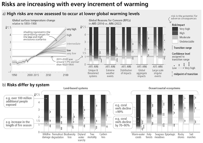
Burning embers for specific land-based or ocean/coastal-based systems are shown in Figure 2.9 panel (b). Warm-water corals are already at high risk at 1.1°C global warming. They are projected to reach very high risk at a global warming of 1.5°C, declining by 70–90 per cent. This rises to a decline of 90 per cent at 2°C global warming. Moderate risk is given to wildfires at today’s level of warming. This transitions to very high risk at 3°C global warming. At over 4°C global warming, for example, an extra 100 million more people will be exposed to wildfires compared to present levels.Footnote ⁶⁶

2.4.5 Regional Changes and Risks

Looking ahead, all regions of the world will experience further climate changes – with changes ratcheting up with every increase in global temperatures.Footnote ⁶⁸ The IPCC reports dedicate hundreds of pages towards assessing regional climate changes and risks, which are insufficiently summarised in this chapter. Outreach material, such as the Working Group I and II’s Regional FactsheetsFootnote ⁶⁹ or the Reports’ Technical Summaries provide a much more detailed analysis of regional changes and risks. Additionally, the IPCC Interactive Atlas allows users to explore the different climate changes in regions of their interest.Footnote ⁷⁰

Each region is unique and affected by climate change in its own way, but every region will increasingly experience multiple and concurrent climate changes: the greater the warming, the larger and more widespread the changes. Changes will be more widespread at 2°C compared to 1.5°C global warming and even more widespread and/or pronounced for higher warming levels.Footnote ⁷¹

Figure 2.10 shows projected changes in annual mean temperature (panel (b)), precipitation (panel (c)), and total soil moisture (panel (d)) at 1.5°C, 2°C, and 4°C global warming compared to 1850–1900 baseline levels. It shows that all regions will experience increases in heat-related climate changes such as heatwaves and decreases in cold-related changes such as cold snaps. Across warming levels, land areas warm more than ocean areas, and the Arctic and Antarctica warm more than the tropics. Precipitation is projected to increase over high latitudes, the equatorial Pacific, and parts of the monsoon regions, but decrease over parts of the subtropics and in limited areas of the tropics. A number of regions in North-Western, Central, and Eastern North America, Arctic regions, North-Western South America, Northern and Central Western Europe, Siberia, Central, South, and East Asia, Southern Australia, and New Zealand will experience decreases in snow and ice or increases in pluvial/river flooding. Across warming levels, changes in soil moisture largely follow changes in precipitation but also show some differences due to the influence of evapotranspiration. Many regions in Southern Africa, the Mediterranean, North Central America, Western North America, the Amazon regions, South-Western South America, and Australia will experience increases in drought, aridity, and weather conducive to triggering and sustaining wildfires. This will affect a wide range of sectors, including agriculture, forestry, health, and ecosystems. Currently, there is lower understanding of past and future changes in some of the damaging hazards such as hail, ice storms, storms, sand and dust storms, heavy snowfall, mudslides, and avalanches. This does not mean that they will not be affected by climate change. Rather, it means that their impacts are not currently able to be fully resolved by climate or impact models and do not benefit from long and homogeneous observations.Footnote ⁷²

Figure 2.10 Changes in annual mean surface temperature, precipitation, and soil moisture. Panel (a): Comparison of observed and simulated annual mean surface temperature change. The left map shows the observed changes in annual mean surface temperature in the period 1850–2020 per °C of global warming (°C). White indicates areas where time coverage was 100 years or less and thereby too short to calculate a reliable magnitude. The right map is based on model simulations and shows change in annual multi-model mean simulated temperatures at a global warming level of 1°C. Panel (b): Simulated annual mean temperature change (°C). Panel (c): Precipitation change (%). Panel (d): Total column soil moisture change at global warming levels of 1.5°C, 2°C, and 4°C.Footnote ⁷⁴

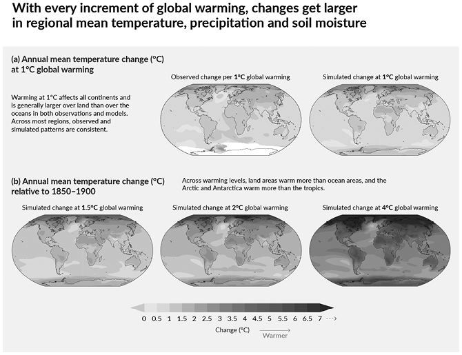
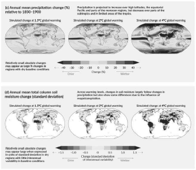
Figure 2.11 gives examples of regional key risks with sufficient data and understanding to assess the risk with at least medium confidence (as characterised by IPCC). In some cases, it is possible to apply a ‘burning ember’ assessment.Footnote ⁷³ Risks in Africa include species extinction, food security risks, marine ecosystem threats, health impacts, and economic decline. Asia risks involve urban infrastructure damage, biodiversity loss, coral bleaching, fishery declines, and food/water security challenges. North America risks encompass health impacts, ecosystem degradation, water scarcity, food security threats, and risks to coastal areas. Central and South America risks include water security, health impacts, coral reef degradation, food security threats, and damages from natural disasters. Australia risks encompass coral reef degradation, coastal loss, agriculture decline, heat-related issues, and loss of alpine biodiversity. Small Islands risks will be biodiversity loss, threats to lives and assets, economic decline, and water security issues. Finally, in Europe, the risks involve flooding, health problems, disruptions to ecosystems, water scarcity, and crop production losses.Footnote ⁷⁵

Figure 2.11 Synthetic diagrams of regional key risks. Diagrams show the change in the levels of impacts and risks assessed for global warming of 0–5°C global surface temperature change relative to pre-industrial period (1850–1900) over the range. Key risks are identified based on the magnitude of adverse consequences (pervasiveness of the consequences, degree of change, irreversibility of consequences, potential for impact thresholds or tipping points, potential for cascading effects beyond system boundaries); likelihood of adverse consequences; temporal characteristics of the risk; and ability to respond to the risk, for example, by adaptation. The full set of 127 assessed global and regional key risks is given in WGII Chapter 17 Supplementary Material Section SM16.7. The development of synthetic diagrams for Small Islands, Asia, and Central and South America were limited by the availability of adequately downscaled climate projections, with uncertainty in the direction of change, the diversity of climatologies and socioeconomic contexts across countries within a region, and the resulting low number of impact and risk projections for different warming levels. Absence of risks diagrams does not imply absence of risks within a region.Footnote ⁷⁶

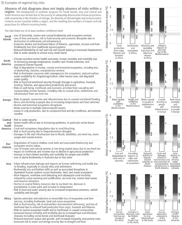
2.4.6 Risks Associated with Overshooting Global Warming of 1.5°C

Every increment of global warming increases climate changes and negative consequences on ecosystems and society. Therefore, if global temperatures were to exceed a warming level, even if only temporarily, many human and natural systems would face additional severe risks compared to a future where global temperatures always remained below that warming level. A temporary overshoot of 1.5°C is a feature of the most ambitious emission pathway (SSP1-1.9, overshooting by ~0.1°C) discussed in Section 2.5. The extent to which severe risks are increased depends on, among other things, the magnitude and duration of a warming level being exceeded. The higher the magnitude or the longer the duration of this ‘overshoot’, the more ecosystems and societies are exposed to greater and more widespread climate changes, such as higher risks to infrastructure, low-lying coastal settlements, and associated livelihoods. Overshooting 1.5°C will result in severe risks and irreversible impacts in many ecosystems with low resilience, such as polar, mountain, and coastal ecosystems. Affected ecosystems will be impacted by temperature increase and extreme events, ice-sheet melt, glacier melt, or accelerating and higher committed sea level rise. Irreversible impacts include extinction of species, loss of coral reefs, and loss of human life.Footnote ⁷⁷

Additionally, some of the adverse impacts that occur during a period of overshoot may cause additional warming via feedback mechanisms that would make the return even more challenging. Such impacts and their feedback mechanism include increased wildfires, mass mortality of trees, drying of peatlands, permafrost thawing, weakening natural land carbon sinks, and increasing releases of greenhouses gases.Footnote ⁷⁸

Temporarily overshooting a global warming level is a relatively new area of research and has limited model-based assessments on how the climate responds to and the impacts of an overshoot. Observations and current understanding of climate processes support the current understanding of the implications of an overshoot but further research would allow assessments to be more robust and comprehensive.

2.4.7 The Role of the Land and Ocean Removing Atmospheric Carbon Dioxide

Finally, climate change affects the natural removal of carbon from the atmosphere, predominantly by land vegetation and ocean, which removes roughly half of the carbon dioxide that humans emit to the atmosphere. This fraction of carbon dioxide removal has remained relatively stable over the past sixty years (at roughly 56 per cent). While human activities emitted more and more carbon dioxide into the atmosphere, the land vegetation and ocean also removed more carbon dioxide. This has led to the oceans becoming more acidic, because when carbon dioxide dissolves in water, it reacts to make the seawater more acidic. Climate modelling shows, however, that if more and more carbon dioxide is emitted into the atmosphere, the relative amount being naturally removed by the land vegetation and ocean would decline. For example, the scenario where carbon dioxide emissions are ambitiously mitigated and global temperatures are kept to below 1.5°C by the end of the century (SSP1–1.9) shows a 70 per cent removal of carbon dioxide by the land and ocean. Conversely, the scenario where carbon dioxide emissions remain relatively high in the future (SSP3–7.0) shows that the land and ocean will only remove 44 per cent from the atmosphere. The bottom line is that nature will ‘help’ less if more carbon dioxide is emitted in the future compared to if emissions in the future are reduced.Footnote ⁷⁹

2.5.1 Paris Agreement: Are We on Track?

Current emissions reduction pledges under the Paris Agreement, known as countries’ NDCs, are ‘woefully insufficient’ to meet the treaty’s long-term temperature goal.Footnote ⁸⁰ The IPCC highlighted in 2022 that NDCs announced before COP26 in 2021 would lead to warming exceeding 1.5°C in the twenty-first century. Unless combined with a rapid acceleration of efforts to reduce emissions after 2030, they would also result in 2°C of warming being exceeded.Footnote ⁸¹

Estimating the alignment of NDCs or climate policies with temperature goals is an inherently dynamic exercise, as countries are expected to regularly update their NDCs as part of the Paris Agreement’s five-yearly ratcheting cycles and the number of national climate policies can change at any time. The snapshots provided by scientific assessments such as those of the IPCC will therefore only be valid over a limited amount of time. Other authoritative initiatives provide more regular updates. For example, UNEP publishes their Emissions Gap Report yearly,Footnote ⁸² providing a synthesis of the most up-to-date information about where emissions are heading under the NDCs and as a result of policies that countries are implementing domestically.

The 2023 edition of the UNEP Emissions Gap Report indicated that NDCs available at that point in time would only hold global warming to 2.5–2.9°C over the course of the twenty-first century (with 66 per cent likelihood). Moreover, domestic climate policies were falling short of achieving these insufficient NDCs and would, without further strengthening, hold global warming to 3.0°C only.Footnote ⁸³ This assessment by UNEP is updated annually and is expected to change as new NDCs are submitted, and domestic policies are taken up or rolled back.Footnote ⁸⁴

2.5.2 How to Stabilise Global Temperature

2.5.2.3 Carbon Budgets

The near-linear relationship between cumulative anthropogenic carbon dioxide emissions and global warming implies that limiting global temperature increase to a specific level requires limiting overall carbon dioxide emissions to within a carbon budget. Such carbon budgets have been estimated (Table 2.1) and are regularly updated with more recent data.Footnote ⁹¹ Carbon budget estimates depend critically on the level of global warming that is to be avoided (e.g. 1.5°C, 1.7°C, or 2.0°C), the likelihood with which this level of warming is to be avoided (50 per cent, 66 per cent, 90 per cent, or higher), and assumptions about how deeply other greenhouse gases are mitigated.Footnote ⁹⁴ Irrespective of the choices that can be made regarding the likelihood of avoiding a given level of warming and the reductions in other greenhouse gas emissions, the remaining carbon budgets for 1.5°C and 2°C are very small.

Table 2.1 Historical carbon dioxide emissions and estimates of remaining carbon budgets. Estimated remaining carbon budgets are calculated from the beginning of 2020 and extend until global net-zero CO₂ emissions are reached. They refer to CO₂ emissions, while accounting for the global warming effect of non-CO₂ emissions. Global warming in this table refers to human-induced global surface temperature increase, which excludes the impact of natural variability on global temperatures in individual years.Footnote ⁹²

Global warming between 1850–1900 and 2010–2019 (°C)		Historical cumulative CO2 emissions from 1850 to 2019 (GtCO2)
1.07 (0.8–1.3; likely range)		2390 (± 240; likely range)
Approximate global warming relative to 1850–1900 until temperature limit (°C)Footnote a	Additional global warming relative to 2010–2019 until temperature limit (°C)	Estimated remaining carbon budgets from the beginning of 2020 (GtCO2)Likelihood of limiting global warming to temperature limitFootnote b					Variations in reductions in non-CO2 emissionsFootnote c
		17%	33%	50%	67%	83%
1.5	0.43	900	650	500	400	300	Higher or lower reductions in accompanying non-CO2 emissions can increase or decrease the values on the left by 220 GtCO2 or more
1.7	0.63	1450	1050	850	700	550
2.0	0.93	2300	1700	1350	1150	900

^a Values at each 0.1°C increment of warming are available in Tables TS.3 and 5.8.

^b This likelihood is based on the uncertainty in transient climate response to cumulative CO₂ emissions (TCRE) and additional Earth system feedbacks and provides the probability that global warming will not exceed the temperature levels provided in the two left columns. Uncertainties related to historical warming (± 550 GtCO₂) and non-CO₂ forcing and response (± 220 GtCO₂) are partially addressed by the assessed uncertainty in TCRE, but uncertainties in recent emissions since 2015 (± 20 GtCO₂) and the climate response after net-zero CO₂ emissions are reached (± 420 GtCO₂) are separate.

^c Remaining carbon budget estimates consider the warming from non-CO₂ drivers as implied by the scenarios assessed in SR1.5. The Working Group Ill Contribution to AR6 will assess mitigation of non-CO₂ emissions.

Figure 2.12 illustrates how a failure to reduce carbon dioxide emissions from today until 2030 will exhaust the remaining carbon budget for keeping warming to 1.5°C with 50 per cent chance entirely.

Figure 2.12 Visual representation of historical carbon dioxide emissions and estimates of remaining carbon budgets for keeping warming to 1.5°C and 2°C with different levels of probability. The lower bars show how quickly the remaining carbon budgets are depleted if global CO₂ emissions do not decline from current (in this case 2019) levels or if all emissions embedded in current and planned fossil fuel infrastructure are considered.Footnote ⁹³

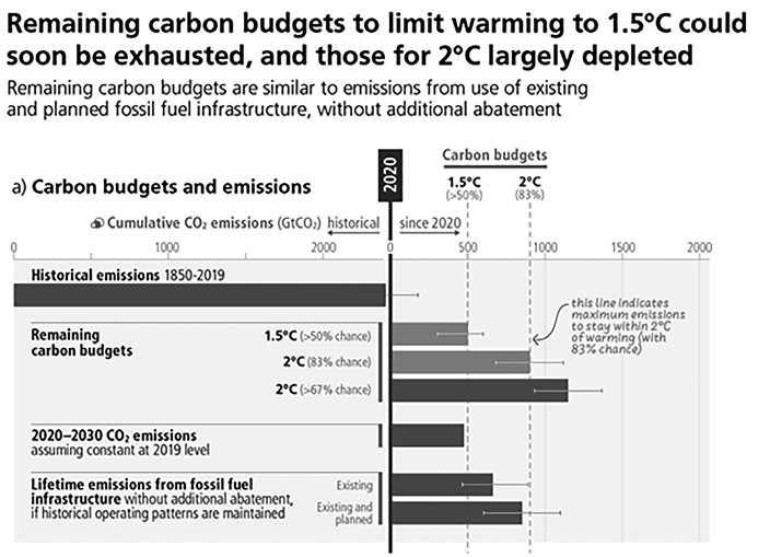
Carbon budgets describe geophysical limits to how much carbon dioxide society can emit while keeping warming to a specified temperature level. To understand how we can stay within these carbon budget limits, they are used as inputs into analyses of how society can transform while meeting global energy, food, and other needs. The models used to explore these transformations are called IAMs (see Section 2.4.1). These models make assumptions about future socioeconomic developments (which are often structured along a specific SSP) and the level of desired climate change mitigation (often defined by a maximum carbon budget that can be emitted). The socioeconomic assumptions include aspects of economic growth, inequality, and availability and characteristics of technologies, as well as levels of education or population growth. Conditional on these assumptions, IAMs then create emissions scenarios that are consistent with limiting global warming to a specific level and that are considered technically and economically feasible within the socioeconomic context that was assumed. The IPCC provides further tools to understand the feasibility of emissions scenarios, and highlights that this depends on geophysical, economic, technological, socio-cultural, and institutional aspects.Footnote ⁹⁵ Geophysical, economic, and technological aspects of the feasibility of mitigation scenarios are typically covered better by IAMs than aspects of socio-cultural and institutional feasibility which are more subject to societal willingness and capacity for change.

Table 2.2 gives a detailed overview of the key characteristics of different modelled pathways showing how the world could respond to climate change.Footnote ⁹⁶ The table covers projected carbon dioxide and greenhouse gas emission reductions and net-zero timings. Scenarios are clustered into several categories including:

• C1: Limit warming to 1.5°C (>50%) with no or limited overshoot (97 scenarios). This category refers to scenarios that reach or exceed 1.5°C during the twenty-first century with a likelihood of ≤67%, and limit warming to 1.5°C in 2100 with a likelihood of >50%. Limited overshoot refers to exceeding 1.5°C by up to about 0.1°C and for up to several decades. By limiting the maximum likelihood of exceeding 1.5°C, scenarios in this category simultaneously have a likelihood of close to and more than 90 per cent of limiting peak global warming to 2°C throughout the twenty-first century.

• C2: Return warming to 1.5°C (>50%) after a high overshoot (133 scenarios). This category refers to scenarios that exceed warming of 1.5°C during the twenty-first century with a likelihood of >67%, and limit warming to 1.5°C in 2100 with a likelihood of >50%. High overshoot refers to central warming estimates temporarily exceeding 1.5°C global warming by 0.1°C–0.3°C for up to several decades.

• C3: Limit warming to 2°C (>67%) (311 scenarios). This category refers to scenarios that limit peak warming to 2°C throughout the twenty-first century with a likelihood of >67%.

As risks of global warming increase with every additional 0.1°C of warming and the sustainable scale of CDR technologies needed to reverse warming after an overshoot is still speculative, it is clear that scenarios in the C1 category represent the safest climate future. Even within the C1 category there are, however, scenarios that might be undesirable as some of them rely strongly on mitigation measures which might have other societal side effects, such as a reduction in biodiversity if a scenario relies excessively on biomass for energy production or types of afforestation with poor biodiversity.

Table 2.2 Key characteristics of the modelled global emissions pathways. Summary of projected CO₂ and GHG emissions, projected net-zero timings, and the resulting global warming outcomes. Pathways are categorised (C1–C3), according to their likelihood of limiting warming to different peak warming levels in 2100. Values shown are for the median [p50] and 5th–95th percentiles [p5–p95], noting that not all pathways achieve net-zero CO₂ or GHGs.Footnote ⁹⁷

p50 [p5–051]			GHG emissions (GtCO2-eqyr-1)			GHG emissions reductions from 2019 (%)			Emissions milestones
Category [#pathways]	Category/subject label	WGI SSP & WGIII IPs/IMPs alignment	2030	2040	2050	2030	2040	2050	Peak CO2 emissions (% peak before 2100)	Peak GHG emissions (% peak before 2100)	Net-zero CO2 (% net-zero pathways)	Net-zero GHGs (% net-zero pathways)
Modelled global emissions pathways categorised by projected global warming levels. Detailed likelihood definitions are provided in SPM Box 1. The five illustrative scenarios (SSPx yy) considered by AR6 WGI and the Illustrative (Mitigation) Pathways assessed in WGIII are aligned with the temperature categories and are indicated in a separate column. Global emission pathways contain regionally differentiated information. This assessment focuses on their global characteristics.			Projected median annual GHG emissions in the year across the scenarios, with the 5th–95th percentile in brackets. Modelled GHG emissions in 2019: 55 [53–58] GtCO2-eq.			Projected median GHG emissions reductions of pathways in the year across the scenarios compared to modelled 2019, with the 5th–95th percentile in brackets. Negative numbers indicate increase in emissions compared to 2019.			Median 5-year intervals at which projected CO2 & GHG emissions peak, with the 5th-95th percentile interval in square brackets. Percentage of peaking pathways is denoted in round brackets. Three dots (…) denotes emissions peak in 2100 or beyond for that percentile.		Median 5-year intervals at which projected CO2 & GHG emissions of pathways in this category reach net zero, with the 5th–95th percentile interval in square brackets. Percentage of net-zero pathways is denoted in round brackets. Three dots (…) denotes net zero not reached for that percentile.
C1 [97]	limit warming to 1.5°C (>50%) with no or limited overshoot		31 [21–36]	17 [6–23]	9 [1–15]	43 [34–60]	69 [58–90]	84 [73–98]	2020–2025 (100%) [2020–2025]		2050–2055 (100%) [2035–2070]	2095–2100 (52%) [2050–…]
												2070–2075 (100%) [2050–2090]
C1a [50]	… with net-zero GHGs	SSP1–1.9, SP LD	33 [22–37]	18 [6–24]	8 [0–15]	41 [31–59]	66 [58–89]	85 [72–100]				…–… [0%]
C1b [47]	… without net-zero GHGs	Ren	29 [21–36]	16 [7–21]	9 [4–13]	48 [35–61]	70 [62–87]	84 [76–93]				[…–…]
C2 [133]	return warming to 1.5°C (>50%) after a high overshoot	Neg	42 [31–55]	25 [17–34]	14 [5–21]	23 [0–44]	55 [40–71]	75 [62–91]	2020–2025 (100%) [2020–2030] [2020–2025]		2055–2060 (100%) [2045–2070]	2070–2075 (87%) [2055–…]
C3 [311]	limit warming to 2°C (>67%)		44 [32–55]	29 [20–36]	20 [13–26]	21 [1–42]	46 [34–63]	64 [53–77]	2020–2025 (100%)		2070–2075 (93%) [2055–…]	…–… (30%) [2075–…]
									[2020–2030]		[2020–2025]
C3a [204]	… with action starting in 2020	SSP1–2.6	40 [30–49]	29 [21–36]	20 [14–27]	27 [13–45]	47 [35–63]	63 [52–76]	2020–2025 (100%) [2020–2025]		2070–2075 (91%) [2055–…]	…–… (24%) [2080–…]
C3b [97]	… NDCs until 2030	GS	52 [47–56]	29 [20–36]	18 [10–25]	5 [0–14]	46 [34–63]	68 [56–82]	2020–2025 (100%)[2020–2030]		2065–2070 (97%)[2055–2090]	…–… (41%)[2075–…]

Based on global modelled pathways that limit warming to 1.5°C (>50%) with no or limited overshoot and in those that limit warming to 2°C (>67%) and assume immediate action, greenhouse gas emissions will reach their peak sometime between 2020 and, at the latest, before 2025. For these scenarios rapid and deep greenhouse gas emissions reductions continue through 2030, 2040, and 2050. Table 2.2 highlights that net global greenhouse gas emissions need to fall from 2019 levels by 27 per cent by 2030 and 63 per cent by 2050 for category C3a, that is, limit warming to 2°C (>67%) and assuming immediate action. While for category C1, it should reduce by 43 per cent by 2030 and 84 per cent by 2050. In pathways with larger overshoot – C2 – greenhouse gas emissions are reduced by 23 per cent in 2030 and by 75 per cent in 2050. These reduction percentages are median estimates surrounded by ranges that illustrate choices about the distribution of emissions reductions over time (see Table 2.2). If weaker emissions reductions are assumed by 2030, stronger emissions reductions will be required later to remain within the same carbon budget and limit warming below the same temperature limit.

Global net-zero greenhouse gas emissions, when measured in terms of their global warming potential over a 100-year period (GWP–100), are expected to be achieved sometime between 2095 and 2100 for C1. Pathways that reach net-zero greenhouse gas emissions before 2100 (which also includes roughly 90% of pathways that bring global warming back down to 1.5°C after experiencing a high overshoot (>0.1°C) by 2100) typically have a time gap of twelve to fourteen years (7–39) years, between reaching net-zero carbon dioxide emissions and reaching net-zero greenhouse gas emissions.Footnote ⁹⁸

Global modelled emission pathways, including those based on cost effective approaches, contain regionally differentiated assumptions and outcomes, and have to be assessed with the careful recognition of these assumptions. Most do not make explicit assumptions about global equity, environmental justice, or intra-regional income distribution. See also Section 2.2.1.

2.5.3 Mitigation Actions

The IPCC defines mitigation as a human intervention to reduce emissions or enhance the sinks of greenhouse gases. Mitigation measures include technologies, processes, or practices that reduce emissions.Footnote ⁹⁹ Modelled pathways that limit warming to 1.5°C with no or limited overshoot assume immediate and ambitious mitigation action this decade. These actions fall broadly into the following categories: deployment of low- or zero-emission technologies, reducing and changing demand through infrastructure design and access, socio-cultural and behavioural changes, and increased technological efficiency and adoption.Footnote ¹⁰⁰

Figure 2.13 shows that multiple mitigation and adaptation options are already available. These solutions span across a number of sectors, including energy systems, industry, transport, buildings, agriculture, forestry, and land-use, that have been effectively implemented in many parts of the world (see Section 2.6 for more information on adaptation).Footnote ¹⁰¹

Figure 2.13 Multiple opportunities for scaling up climate action. Panel (a): presents selected mitigation and adaptation options across different systems. Left – climate responses and adaptation options assessed for their multidimensional feasibility at global scale, in the near term and up to 1.5°C global warming. Six feasibility dimensions (economic, technological, institutional, social, environmental, and geophysical) were used to calculate the potential feasibility of climate responses and adaptation options, along with their synergies with mitigation. For potential feasibility and feasibility dimensions, the figure shows high, medium, or low feasibility. Synergies with mitigation are identified as high, medium, and low. Right – an overview of selected mitigation options and their estimated costs and potentials in 2030. The potential (horizontal axis) is the quantity of net GHG emission reduction that can be achieved by a given mitigation option relative to a specified emission baseline. The baseline used consists of current policy (around 2019) reference scenarios from the AR6 scenarios database (25–75 percentile values). Potentials are broken down into cost categories (see Net lifetime of cost options in the bottom right of panel (a)). The uncertainty in the total potential is typically 25–50%. Panel (b): displays the indicative potential of demand-side mitigation options for 2050. The left-pointing arrows represent the demand-side emissions reductions potentials. The range in potential is shown by a line connecting dots displaying the highest and the lowest potentials reported in the literature. The bottom row shows how demand-side mitigation options in other sectors can influence overall electricity demand. The dark grey bar shows the projected increase in electricity demand above the 2050 baseline due to increasing electrification in the other sectors. This projected increase in electricity demand can be avoided through demand-side mitigation options in the domains of infrastructure use and socio-cultural factors that influence electricity usage in industry, land transport, and buildings (indicated by the left-pointing arrow).Footnote ¹⁰⁹

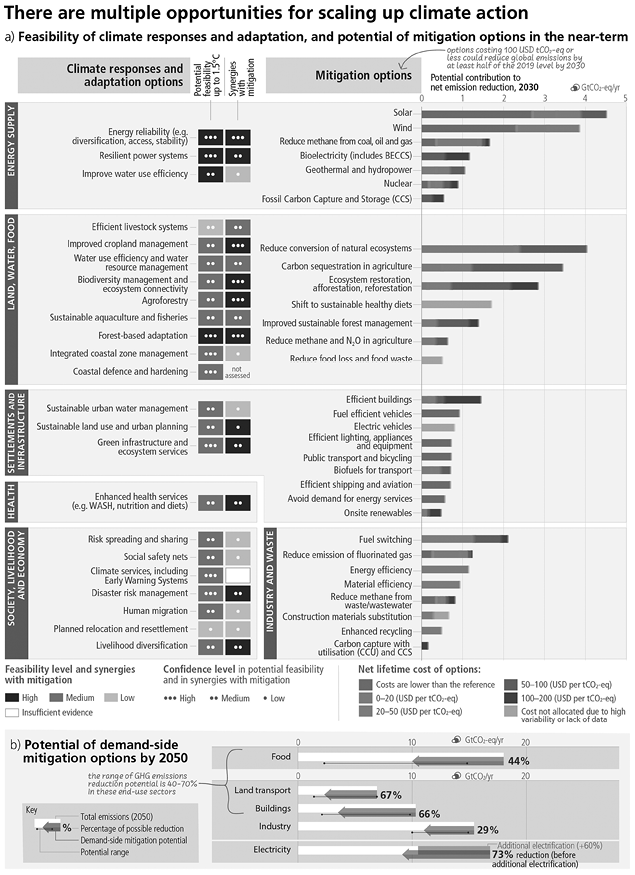
Phasing out fossil fuels merits especially urgent attention, as current levels of fossil fuel consumption and new investments in fossil fuels are inconsistent with 1.5°C or even 2°C pathways (see Figure 2.12). Projections show that new investments in fossil fuels are not consistent with meeting the goals of the Paris Agreement and the achievement of Sustainable Development Goals, leading to substantial economic losses from stranded assets while also delaying the development of low carbon sectors and infrastructure.Footnote ¹⁰² Immediate action to phase out fossil fuels and reduce emissions more broadly would: reduce and avoid the reliance on risky and less known CDR methods; reduce or avoid climate damages from high-temperature overshoot; and bring long-term gains for the economy, as well as earlier benefits of avoided climate change impacts.Footnote ¹⁰³

Many of the solutions aligned with 1.5°C pathways are transformative. For energy systems, for example, this would imply an ambitious transformation from current polluting systems towards electricity systems that emit no or very low carbon dioxide emissions. This would involve moving away from fossil fuel use, increasing energy conservation and energy efficiency, and increased use of renewable energy and higher electrification.Footnote ¹⁰⁴ However, such a transition is complex and challenging and may result in distributional consequences within and between countries. Such transitions need to be carefully managed.

Food systems, including agriculture, processing, transport, and consumption of food also have a significant impact on the climate system, as well as on biodiversity, soil quality, and human health. Diets that include high amounts of plant proteins and have low meat and dairy are associated with lower greenhouse gas emissions and bring higher benefits to human health and to the planet. Realising the full mitigation potential from the food system requires change at all stages from producer to consumer and waste management, which can be facilitated through integrated policy packages.Footnote ¹⁰⁵

In addition, there is a need to identify policies and actions that can reduce emissions intensive consumption or what is referred to as status consumption. Choices made by policymakers, citizens, the private sector, and other stakeholders all influence societies’ development pathways.Footnote ¹⁰⁶

2.5.4 Policies, Legislation, and Enabling Conditions

Many countries, both developed and developing, have announced plans to achieve net-zero greenhouse gas (or carbon dioxide) emissions by or around mid century. These targets now cover 90 per cent of global emissions, compared to 49 per cent in 2010. Direct and indirect climate legislation has also steadily increased and this is supported by a growing list of financial investors. But these targets often lack clear definitions and roadmaps for achievement. The UNFCCC, Kyoto Protocol, and Paris Agreement are supporting rising levels of national ambition and encouraging development and implementation of climate policies, but large gaps remain.Footnote ¹⁰⁷

Accelerated international financial cooperation is a critical enabler of low greenhouse gas and just transitions but the current tracked financial flows to achieve mitigation goals across all sectors and regions fall short of the finance levels needed. These gaps are largest in developing countries. Developing countries need increased financial support from developed countries and other sources to enhance their mitigation actions and address financial inequities and impacts related to climate change. Technology transfer and capacity building are also crucial for these countries to transition to low-emission systems.Footnote ¹⁰⁸