


1. INTRODUCTION
A better understanding of the physics governing ice deformation is critical both for predicting the dynamic response of ice sheets to climate forcing (e.g. Vaughan and Arthern, Reference Vaughan and Arthern2007), and for interpreting paleo-climate records from ice cores (e.g. Alley and others, Reference Alley1997; Waddington and others, Reference Waddington, Bolzan and Alley2001) and ice-sheet internal layer measurements (e.g. Waddington and others, Reference Waddington, Neumann, Koutnik, Marshall and Morse2007; Martin and others, Reference Martin, Gudmundsson, Pritchard and Gagliardini2009). A key constraint on the flow of ice sheets is crystal orientation fabric (COF), the distribution of crystal orientations within the ice (e.g. Alley, Reference Alley1988; Azuma, Reference Azuma1994; Mangeney and others, Reference Mangeney, Califano and Hutter1997).
Because ice crystals are elastically anisotropic, the speed of an elastic wave traveling through ice is affected by COF. By measuring sonic waves in a borehole, it is possible to constrain the types of fabric that prevail in the surrounding ice and to determine parameters describing that fabric. This method is readily implemented at sites where boreholes remain open after core drilling, and uniquely complements other methods for measuring COF.
In this paper we present background on COF, wave propagation in ice, and sonic logging in general. We review how sonic logging can be used to measure COF in ice, and constrain the information that can and cannot be gained with the method. With results from sonic and thin-section studies at the West Antarctic Ice Sheet Divide ice core site (WAIS-D), we demonstrate the relationship between sonic wave speeds and several fabric parameters, and present a framework for interpreting existing sonic data, as well as a prescription for future developments in sonic logging.
2. COF IN ICE SHEETS
Naturally occurring ice is an aggregate of grains that range from less than a millimeter to centimeters in size. Each of these grains has a layered molecular structure (crystal) that results in anisotropic elasticity (Fletcher, Reference Fletcher1970, p. 271) and viscoplasticity (Duval and others, Reference Duval, Ashby and Anderman1983). Consequently, the deformation rate of an ice-grain aggregate is strongly constrained by its COF. Under a given stress regime, the strain rate of ice can vary by an order of magnitude depending on its COF (e.g. Castelnau and others, Reference Castelnau1998; Thorsteinsson and Waddington, Reference Thorsteinsson and Waddington2002). Accounting for COF can substantially alter the results of ice-sheet modeling (Pettit and others, Reference Pettit, Thorsteinsson, Jacobson and Waddington2007; Seddik and others, Reference Seddik, Greve, Placidi, Hamann and Gagliardini2008).
2.1. Representations of ice fabrics
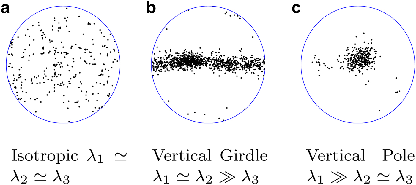
The orientation of a single ice crystal can be described by the direction of its c-axis, the axis that is normal to its crystalline planes (basal planes). The distribution of c-axis orientations is conventionally displayed as a Schmidt projection, in which each dot represents the orientation of a crystal c-axis; the distance from center describes the zenith (from vertical) angle, whereas azimuths within the plane of the plot describe the azimuthal (in the horizontal plane) angle of each c-axis (Fig. 1). Although young ice at the top of an ice sheet is often near-isotropic (random distribution of crystal orientations, Fig. 1a), strain and recrystallization (both of which are influenced by temperature and impurity content) lead to strongly anisotropic COF at sufficient (1000–2000 m) depths (Gow and Williamson, Reference Gow and Williamson1976; Alley, Reference Alley1988; Thorsteinsson and others, Reference Thorsteinsson, Kipfstuhl and Miller1997). Both vertical-pole (Fig. 1c) and vertical-girdle (Fig. 1b) fabrics, as well as abrupt changes between the two have been observed in Greenland (Herron and Langway, Reference Herron and Langway1982; Gow and others, Reference Gow1997; Wang and others, Reference Wang2002) and Antarctica (Lipenkov and others, Reference Lipenkov, Barkov, Dural and Pimenta1989; Azuma and others, Reference Azuma1999; Gusmeroli and others, Reference Gusmeroli, Pettit, Kennedy and Ritz2012).
Schmidt plots for typical fabric types in ice. C-axis data are from thin-section records of the WAIS-Divide ice core at (a) 540 m, (b) 2500 m and (c) 3205 m depth. Fabric parameters λ i (eigenvalues) are explained in subsequent sections. (a) Isotropic λ 1 ≃ λ 2 ≃ λ 3 (b) Vertical Girdle λ 1 ≃ λ 2 ≫ λ 3 (c) Vertical Pole λ 1 ≫ λ 2 ≃ λ 3.
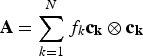
Fabric eigenvalues are the most prevalent parameterization for COF in recent glaciological literature. Eigenvalues are calculated from the following tensor:
 $${\bf A} = \sum\limits_{k = 1}^N f_k {\bf c}_{\bf k} \otimes {\bf c}_{\bf k} $$
N is the number of grains, f k is the volume weight of the k th grain, ck is a unit vector in the direction of each associated crystal c-axis and ⊗ indicates the outer matrix product (Woodcock, Reference Woodcock1977). Properties for these eigenvalues include:
 $$\eqalign{& \lambda _1 + \lambda _2 + \lambda _3 = 1 \cr & \lambda _1 \ge \lambda _2 \ge \lambda _3} $$
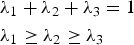
For an isotropic fabric, λ 1 = λ 2 = λ 3. For a pure pole (all c-axes aligned along one vector), λ 1 = 1; λ 2 = λ 3 = 0. For pure girdle fabrics (all c-axes distributed evenly throughout one plane): λ 1 = λ 2 = 0.5; λ 3 = 0.
Grain volumes cannot be measured directly in a thin section. Gagliardini and others (Reference Gagliardini, Durand and Wang2004) showed that the area a k of the k th grain within a thin section is a good representation of the grain's volume among the represented grains. A characterization of ice fabric with area weighting 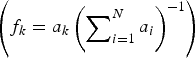 $\left( {f_k = a_k \left( {\sum\nolimits_{i = 1}^N a_i} \right)^{ - 1}} \right)$ provides better estimates for fabric properties than equal-area weighting (f k = N −1).
We use the following parameters to track fabric development into pole and girdle types:
 $${\rm Pole \ Parameter} \equiv \lambda _1 - \lambda _2 $$
 $${\rm Girdle \ Parameter} \equiv 2(\lambda _2 - \lambda _3 )$$
Both parameters range from zero to unity as a fabric develops from isotropic to a perfect form of their respective types. Any pole fabric with the property that λ 1 > λ 2 = λ 3 will have a girdle parameter of zero, and likewise any girdle fabric with the property that λ 1 = λ 2 > λ 3 will have a pole parameter of zero. This means that these parameters are independent in the sense that pole or girdle development will not affect the fabric's girdle or pole parameter, respectively.
2.2. Measuring COF
Established methods for measuring crystal fabric include thin-section analyses (e.g. Gow and Williamson, Reference Gow and Williamson1976), seismic reflections (Bentley, Reference Bentley and Crary1971; Horgan and others, Reference Horgan, Anandakrishnan, Alley, Burkett and Peters2011), radar reflections (Matsuoka and others, Reference Matsuoka2003; Fujita and others, Reference Fujita, Maeno and Matsuoka2006) and sonic logging (Bentley, Reference Bentley1972; Kohnen and Gow, Reference Kohnen and Gow1979; Anandakrishnan and others, Reference Anandakrishnan, Fitzpatrick and Alley1994). These methods have complementary strengths and weaknesses.
Thin-section analyses provide the most detailed measurement of COF in small volumes, but are impractical for measuring abrupt fabric variations throughout extensive depth domains. In addition, because average grain sizes generally increase with age (e.g. Duval and Lorius, Reference Duval and Lorius1980), decreasing numbers of grains in a thin section make this method statistically less reliable deeper in an ice core – the fabric sampled in the thin section becomes less representative of the surrounding volume.
Seismic and radar methods allow users to remotely characterize ice properties throughout the depth of an ice sheet. Abrupt changes in COF in the vertical direction can be inferred with seismic and radar reflections, and azimuthal anisotropy in the horizontal plane can be inferred with birefringence (Matsuoka and others, Reference Matsuoka, Power, Fujita and Raymond2012). These methods do not provide a detailed characterization of local fabric or an accurate measurement of length scale over which transitions occur. Nevertheless, these methods are vital to detect spatial patterns of COF in ice sheets, and to extend ice core-based knowledge of COF (mainly from ice domes where ice cores are drilled) to COF that occurs throughout large volumes in various flow regimes.
Sonic logging is an efficient method for measuring depth-continuous profiles of COF in the vicinity of a borehole. The method was first implemented in ice by Bentley (Reference Bentley and Crary1971), and was used to measure crystal fabric by Gusmeroli and others (Reference Gusmeroli, Pettit, Kennedy and Ritz2012). Sonic logs that measure the velocity of compressional (P) waves traveling vertically along a borehole wall were effective for measuring vertical clustering of ice-crystal c-axes in regions where vertical-pole fabrics prevail. More-advanced methods are necessary to detect and quantify vertical-girdle fabrics.
3. ELASTIC WAVES IN ICE
3.1. Single crystal
A single ice crystal is hexagonally symmetric in its elasticity. A number of values for the stiffness tensor have been reported in the literature and were summarized by Gusmeroli and others (Reference Gusmeroli, Pettit, Kennedy and Ritz2012). In each case, the crystal is more resistant to longitudinal stress along its c-axis and to shear stress in the transverse plane; for a crystal with its c-axis aligned with the z-axis this means that C zzzz > C xxxx = C yyyy, and C xyxy > C yzyz = C xzxz, with C defined so that  ${\sigma}_{ij} = C_{ijkl} {\kern 1pt} {\epsilon} _{kl} $ where fσ is stress and f ε is strain. Using the summation convention (e.g. Mase and Mase, Reference Mase and Mase1999, p. 5), this stiffness tensor can be viewed in a rotated coordinate system according to the rule:
 $$C^{\prime}_{ijpn} = a_{iq} a_{\,js} a_{\,pk} a_{nm} C_{qskm} $$
where direction cosines a ij are defined so that  $\hat e^{\prime}_i = a_{ij} \hat e_j $ where $\hat e_i $ and $\hat e^{\prime}_i $ are the coordinate axes in the original and rotated coordinate systems (Mase and Mase, Reference Mase and Mase1999, p. 221).
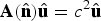
From the stiffness tensor, one can use the Christoffel Equation to find three normal-mode solutions to the elastodynamic wave equation (Aki and Richards, Reference Aki and Richards1980, pp. 177–178). The Christoffel equation is:
 $${\bf A}({ \hat {\bf n}}){\hat {\bf u}} = c^2 {\hat{\bf u}}$$
where  ${ \hat {\bf n}}$ is a unit vector in the direction of wave propagation and
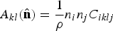 $$A_{kl} ({ \hat {\bf n}}) = \displaystyle{1 \over \rho} n_i n_j C_{iklj} $$
where ρ is the ice density. The three eigenvalue-and-eigenvector pair (c and  ${\hat{\bf u}}$) solutions are the speeds and polarization directions for one compressional-wave and two shear-waves. For analytical solutions, see Bennett (Reference Bennett1968).
3.2. Crystal aggregates
Preceding literature on sonic logging in ice has relied on wave velocity predictions for arbitrary COFs that are the harmonic mean of velocities for waves traveling in the head-wave direction through the individual crystals that compose the aggregate distribution, i.e.
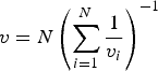 $$v = N\left( {\sum\limits_{i = 1}^N \displaystyle{1 \over {v_i}}} \right)^{ - 1} $$
where N is the number of crystals, v is velocity, and the subscript i denotes an individual crystal. This method is computationally cheap and reasonably intuitive, but has no reasonable physical interpretation for wavelengths greater than the typical grain size, which is always the case for sonic logging in ice.
An alternative method is to average stiffness characteristics for a given fabric distribution and to solve the Christoffel Equation on the aggregate stiffness tensor. While (relatively) computationally expensive, this method can be performed quickly with modern hardware and lends itself to homogeneous-medium wave modeling for which aggregate physical qualities of the ice must be known.
The elastic properties for a crystal aggregate can be estimated by a volume-weighted mean of the orientation-dependent stiffness tensor for each component crystal:
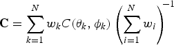 $${\bf C} = \sum\limits_{k = 1}^N w_k C(\theta _k, \phi _k )\left( {\sum\limits_{i = 1}^N w_i} \right)^{\!\! - 1} $$
where C is the aggregate stiffness tensor, and C(θ k, ϕ k) and w k are respectively, the crystal stiffness-tensor and volume of each represented grain. This method, termed the Voigt average, inherently assumes that strain among the grains is uniform. An alternative (Reuss) method takes the harmonic mean of stiffness-matrix components over crystal orientations; the corresponding assumption is uniform stress throughout the aggregate. For the Voigt assumption, inter-grain forces could not be in equilibrium, whereas for the Reuss assumption grains could not fit together. Real-world behavior lies somewhere between the two models (Hill, Reference Hill1952). For our purposes, the two methods produce similar results. We use the Voigt average for its numerical stability around near-zero terms in the stiffness matrix. Both methods predict velocities that are similar, but not equivalent to predictions based on (6).
3.3. Idealized fabric distributions
For modeling purposes, it is often necessary to consider idealized distributions with a parameterized orientation distribution function (Gagliardini and others, Reference Gagliardini, Gillet-Chaulet and Montagnat2009). Lliboutry (Reference Lliboutry1993) proposed a Fisherian distribution defined by the parameter κ:
 $$f_\kappa (\theta ) = \displaystyle{{\kappa e^{\kappa \cos \theta}} \over {e^\kappa - 1}}\sin \theta $$
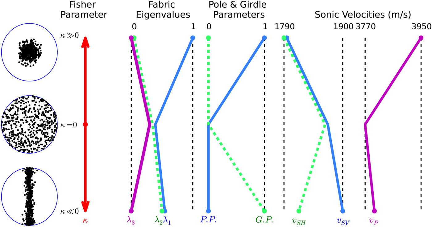
where θ ∈ [0, π/2] is the zenith angle for a crystal. This distribution varies continuously from a strong horizontal girdle (κ ≪ 0), to isotropic (κ = 0), to a strong pole (κ ≫ 0). Vertical girdles can be represented with a coordinate rotation applied to a horizontal-girdle distribution. All idealized distributions used later in this paper are Fisherian. They are generated by controlling the parameter κ, and are described by their eigenvalues, which apply to all distributions. For girdle fabrics, the coordinate system is rotated 90° about a horizontal axis. Eigenvalues for a continuous distribution can be calculated numerically with (1) on a discrete sample of the distribution. Figure 2 shows a qualitative relationship between the Fisher parameter κ and fabric eigenvalues, as well as relationships for fabric parameters and wave velocities that are discussed later in this paper. For our purposes, this distribution was chosen for its qualitative resemblance to real fabrics. The results that follow are similar with other idealized distributions, for example cone angles (Thorsteinsson and others, Reference Thorsteinsson, Kipfstuhl and Miller1997).
A qualitative view of how several fabric parameters vary for a range of idealized fabrics. The left side shows three Fisherian distributions that correspond to positive, zero and negative values for the Fisher parameter κ. Minimum and maximum values for each fabric parameter are printed above their respective graphs. Each colored line shows the values that a parameter takes for a strong pole (top), isotropic (middle) and strong girdle (bottom) fabric, and is labeled with the parameter name in a corresponding color. P.P. and G.P are abbreviations for the pole parameter and girdle parameter.
3.4. Head waves
A sonic source in a fluid-filled borehole in an anisotropic formation (the medium surrounding the borehole, in this case ice) will generate three head waves corresponding to the three plane-wave solutions to the Christoffel Equation: the qP-waves, qS v-waves and qS h-waves. (Sinha and others, Reference Sinha, Norris and Chang1994). The subscripts v and h signify different polarizations for the two shear wave modes. A preceding q (short for quasi) indicates that particle motions are not necessarily parallel or perpendicular to the respective P and S propagation directions. The first-arriving signal from source to receiver is a critically refracted wave; it travels from source to borehole wall as a fluid longitudinal wave (velocity v f), along the borehole wall as a corresponding head wave in the ice and back to the receiver as a fluid longitudinal wave. For the case of isotropic and transverse isotropic formations with a vertical axis of symmetry (e.g. vertical-pole fabrics) or horizontal axis of symmetry (e.g. vertical-girdle fabrics), head-wave particle motions will be parallel or perpendicular to the propagation direction and the three head waves can be referred to simply as P, S v and S h.
Velocities for the three head waves are shown in Fig. 3. All are calculated with (4), (5) and (7), and are based on Fisherian-distribution fabrics (8) with the parameter κ varied to produce various strengths of pole and girdle fabrics. Fabrics are described by the parameter λ 3, which varies from 1/3 to zero for both girdle and pole types.
Predictions for P-waves (top plot) and S-waves (bottom plot) traveling vertically in both pole and vertical-girdle fabrics. Both fabric types are described by the lowest corresponding eigenvalue (λ 3), which varies from λ 3 = 0.33 for isotropic fabric to λ 3 = 0 for a strong pole or girdle. v sv and v sh are the same for pole fabrics.
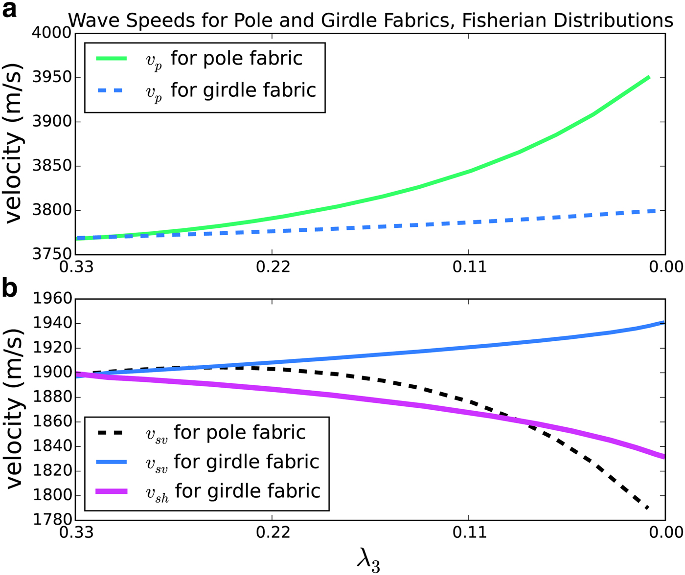
P-wave velocities increase with the strength of a vertical-pole fabric, but are insensitive to vertical-girdle distributions. Shear wave velocities exhibit the opposite behavior for pole fabrics – decreasing with greater concentration of crystal c-axes along the vertical axis. For girdle fabrics, we follow Bennett (Reference Bennett1968) and define the S v and S h polarizations so that respective motions are parallel and normal to the girdle plane. Given this definition, v sv will become progressively greater than v sh as c-axes concentrate toward a vertical plane. This phenomenon is called shear splitting. Note that velocities for the first-arrival shear wave (S v for strong girdles) are relatively insensitive to girdle strength.
3.5. Borehole guided waves
Sonic logging generates several borehole modes that propagate due to interactions between the formation and fluid compressional waves within the borehole. The amplitudes of these modes, as well as the relative prominence of the head waves, are controlled by the borehole geometry, fluid and formation body-wave speeds, and the source frequency and radiation pattern (Crain, Reference Crain2004).
Three borehole modes that are commonly present in sonic-log waveforms are the pseudo-Rayleigh, Stoneley and flexural waves. The pseudo-Rayleigh mode is produced by shear waves within the formation interacting at the margin with direct and reflected fluid compressional waves within the borehole. They are excited in fast (v s > v f, e.g. ice) formations and have speed similar to the S head wave so that the two (S and pseudo-Rayleigh waves) are generally not separable (Paillet and Saunders, Reference Paillet and Saunders1990, p. 66).
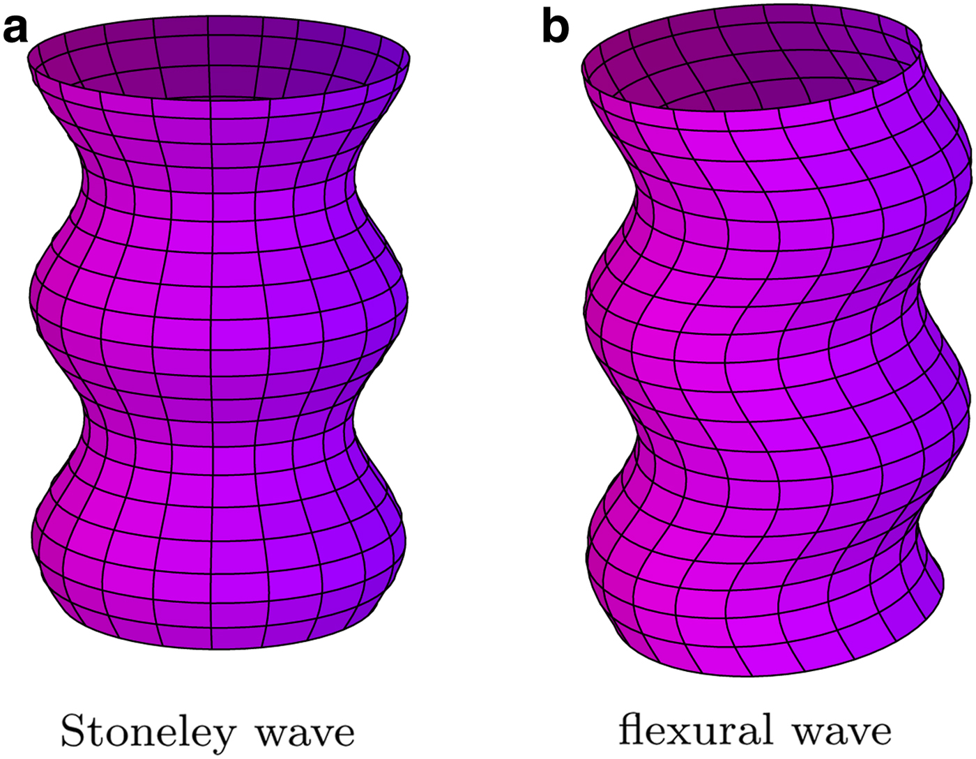
Stoneley and flexural waves are borehole-guided shear modes activated respectively by monopole (isotropic) and dipole (anisotropic) sources (Fig. 4). A monopole source emits an azimuthally isotropic signal, whereas a dipole source emits two opposite-phase signals along opposing azimuths. Both waves are highly dispersive in fast formations, approaching the formation shear-wave velocity for low (~1 kHz) frequencies and the fluid compressional-wave velocity for high (~10 kHz) frequencies (Crain, Reference Crain2004). For low frequencies in an azimuthally anisotropic formation, the flexural wave splits into fast and slow components that correspond to the S v and S h waves in speed and polarization. The Stoneley wave has one intermediate (between S v and S h) speed (Haldorsen and others, Reference Haldorsen2006).
Here we characterize the deformation of an initially cylindrical borehole-surface with a circular cross section for (a) Stoneley and (b) flexural normal modes. Stoneley and flexural modes are activated by monopole and dipole transmitters, respectively. (a) Stoneley wave (b) flexural wave.
4. INSTRUMENT AND METHODS
4.1. Wave-speed measurement
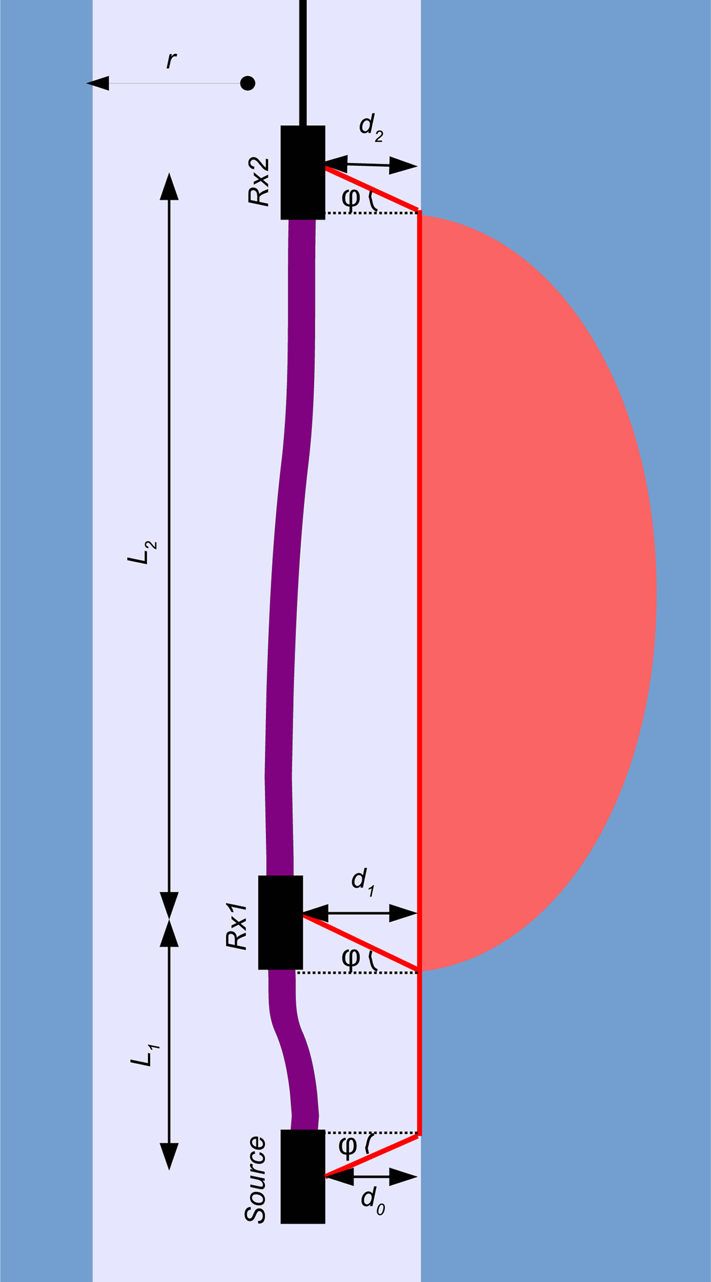
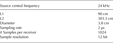
Our tool (Mount Sopris CLP-4877 modified with extended receiver spacing) measures the travel times for P waves that propagate from a monopole signal source, outwards to the surrounding ice, upwards along the ice at the borehole boundary and back through the borehole fluid to each receiver (Fig. 5). Wave transmission is recorded as pressure measurements at 2 µs intervals at each receiver. Properties of the tool are listed in Table 1. Although our tool does not resolve shear-wave arrivals well, much of the following analysis is equally applicable to shear waves. We use the symbol v to describe velocities of head waves that could be P or S types.
Geometry of the sonic tool, borehole, surrounding ice and the propagation path for measured waves. The red, semi-elliptic region represents the Fresnel volume for ice that is sampled by sonic methods. Radius r is measured from the center of the borehole. Waves travel from the source, through the borehole fluid, through ice along the borehole wall and back through the fluid to each receiver. In the ideal case for a centralized tool, d 0 = d 1 = d 2 = r and the propagation geometry is azimuthally isotropic around the borehole.
Properties of Mount Sopris CLP-4877.
From Snell's law in ray theory, the critical angle of refraction for head waves satisfies sin ϕ = v f/v. The borehole-fluid velocity, v f is approximately 1500 m s–1. Within the range of measured values for v p, the refraction angle ϕ is ~20°
Ideally, measurements are made with the tool centered in the borehole, in which case d 0 = d 1 = d 2 and from the wave-propagation geometry:
 $$v = \displaystyle{{L_2} \over T}$$
where v is the velocity of a measured head wave (P or S) that travels along the borehole wall, and T is the difference between arrival times at the two receivers. Centralizers were placed at three positions along the length of the tool in order to align the transmitter and receivers with the borehole central axis. In principle, wave speeds can be calculated from the Source-Rx2 travel time, but in that case the inferred speeds are more sensitive tool-borehole geometry, as well as the fluid P-wave speed.
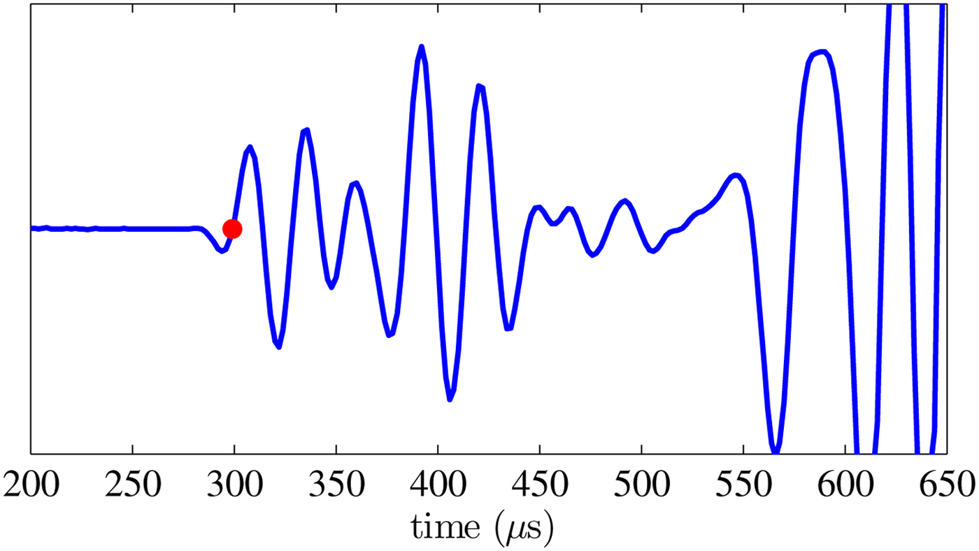
Arrival times are calculated from waveforms at both receivers. The vicinity of the first arrival is detected by comparing two adjacent time averages of signal amplitude over domains equal to half the emission period (1/2ν where ν is the central frequency). Because wave arrivals consistently begin with a pressure ‘dip’, their onset can be located by searching for the region where the second average is significantly less than the first. The arrival time is further refined by selecting the zero-crossing of a linear interpolation of the (discretely sampled) waveform (Fig. 6).
Sample of a wave incident at Rx1. The arrival time (red dot) is chosen as the zero-crossing of the waveform subsequent to the initial dip in recorded pressure.
4.2. Fresnel volume for sampled ice
The propagation time for an elastic wave that travels between two points is affected by the medium in the vicinity of the ray path between the two points. The domain for this effect can be approximated as the region through which diffracted rays will interfere constructively with the direct-path ray, i.e. the combination of all ray paths such that the greatest path length is half a wavelength greater than the shortest. We expand on the treatment for a homogeneous medium from Spetzler and Snieder (Reference Spetzler and Snieder2004) by approximating the Fresnel volume as an elongated toroidal object that wraps around the ice borehole. Calculations are in Appendix A. The Fresnel volume for a head wave between two points separated by a distance L 2 in a borehole of radius r is
 $$V = \pi ab(4a/3 + 2\pi r)$$
where
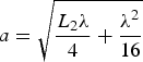 $$a = \sqrt {\displaystyle{{L_2 \lambda} \over 4} + \displaystyle{{\lambda ^2} \over {16}}} $$
and
 $$b = L_2 /2 + \lambda /4$$
 For our experiment, r ≃ 8 cm, L 2 ≃ 300 cm, and λ ≃ 16 cm – this indicates a Fresnel volume of ~2.5 m3, with an elliptical semi-minor axis (penetration depth)  $a\,{\rm \simeq}\, 35{\kern 1pt} \,{\rm cm}$.
4.3. Effects of temperature and pressure
Elastic wave velocities in ice are affected by temperature (Θ) and pressure (p). In order to correct for this effect, the velocities need to be adjusted as
 $$v_{{\rm p}_{\rm c}} = v_{\rm p} - A \cdot (\Theta - \Theta _{\rm r} ) - B \cdot p.$$
where p is pressure, Θ is temperature and Θr is a reference temperature. Following Gusmeroli and others (Reference Gusmeroli, Pettit, Kennedy and Ritz2012), we use A = −2.7 m (S°C)−1, and  $\Theta _{\rm r} \, = \, - 16{\kern 1pt} ^ \circ {\rm C}$ (Kohnen and Gow, Reference Kohnen and Gow1979), as well as B = 0.2 m (s MPa)–1 (Helgerud and others, Reference Helgerud, Waite, Kirby and Nur2009). Both temperature and pressure corrections have been applied to our data (temperature data are from Cuffey and Clow (Reference Cuffey and Clow2014)). Pressure is calculated as p = ρgz where ice density ρ = 920 kg m–3, g = 9.81 m s–2 and z is the depth from surface. Actual densities are lower in the firn (~0–100 m depth (Albert, Reference Albert2015), but we restrict our analysis to lower depths where density is near constant and the relevant change in overburden pressure does not significantly alter the pressure correction, which is small compared with the temperature correction.
4.4. Error analysis
The primary source of error for this sonic method is differing radial location of the two receivers. Consider the case of a tool resting off the borehole central axis with inconsistent spacing between receivers and the borehole wall, as in Figure 5. In this case, the difference between wave arrival times at receivers Rx1 and Rx2 will be:
 $$T = \displaystyle{{d_2 - d_1} \over {v_{\rm f} \cdot \cos \phi}} + \displaystyle{{L_2 + (d_1 - d_2 )\tan \phi} \over v}$$
Recalling that sin ϕ = v f/v, this can be rearranged to
 $$v = \displaystyle{{L_2} \over T}\left( {\displaystyle{{{\hat d} \cdot \cos \phi} \over {T \cdot v_{\rm f}}} - 1} \right)^{ - 1}, $$
where  $\hat d = d_2 - d_1 $.
Note that for the case of a centralized tool (d 1 = d 2) this reduces to (9), and for small  $\hat d$:
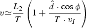 $$v{\rm \simeq} \displaystyle{{L_2} \over T}\left( {1 + \displaystyle{{\hat d \cdot \cos \phi} \over {T \cdot v_{\rm f}}}} \right)$$
 Let v i represent the value for the inferred wave speed. Without knowing the value of  $\hat d$, v i will be calculated as in (9). The inferred wave speed will differ by the true value by the correction term:
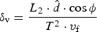 $$\delta _{\rm v} = \displaystyle{{L_2 \cdot {\hat d} \cdot \cos \phi} \over {T^2 \cdot v_{\rm f}}} $$
Given typical values for v p and v f of 3850 m s–1 and 1500 m s–1 respectively, and inserting v = v p and T ≃ L 2/v, this results in an error in inferred waves speed equal to
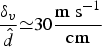 $$\displaystyle{{\delta _v} \over {\hat d}}{\rm \simeq} 30\displaystyle{{{\rm m}\;{\rm s}^{ - 1}} \over {{\rm cm}}}$$
 Wave speeds inferred from a sonic log are influenced strongly by the position of receivers relative to the borehole central axis. Erratic or sustained offset of either receiver will respectively result in random or systematic error for inferred wave speeds; this error will be positive or negative in accordance with the sign of  $\hat d$.
Error from uncertainty in arrival times is relatively small. Letting σ t and σ v respectively, represent errors in arrival-time picks and velocity, then
 $$\displaystyle{{\sigma _{\rm v}} \over {\sigma _{\rm t}}} = \displaystyle{{\sigma _{\rm T}} \over {\sigma _{\rm t}}} \displaystyle{{\sigma _{\rm v}} \over {\sigma _{\rm T}}} = \sqrt 2 \displaystyle{{\partial v} \over {\partial T}} = \sqrt 2 \displaystyle{{L_2} \over {T^2}} = \sqrt 2 \displaystyle{{v_i^2} \over {L_2}} {\rm \simeq} 7\displaystyle{{{\rm ms}^{ - 1}} \over {\mu {\rm s}}},$$
 where  $\sigma _{\rm T} /\sigma _{\rm t} = \sqrt 2 $ because T is the difference between two arrival times. In the least noisy depth regions in our logs, we are able to resolve velocity differences on the order of 1 m s–1 as repeated features in multiple logs (Fig. 8c). Assuming that (resolution-limiting) random error in inferred velocities is primarily from uncertainty in arrival time picks, this indicates an arrival-time uncertainty of no greater than order 0.1 µs, which is significantly smaller than the sampling interval and the source period.
Moderate changes in the tool sampling rate do not strongly affect arrival time uncertainty. Sampling rates of 250 kHz or faster resulted in similar uncertainties, but slower sample rates resulted in a degraded waveform and higher uncertainties in arrival time measurements and velocity estimates. The zero-crossing method for determining wave arrivals is effective for sampling rates of at least 10 times the source frequency.
In summary, our wave-speed measurements are subject to small (order 1 m s–1) random error from arrival-time uncertainty, but large (order 10 m s–1) error from receiver drift. The receiver-drift error will be predominantly systematic, but may behave erratically if a receiver bounces around within the borehole.
5. APPLICATIONS TO THE WAIS DIVIDE
5.1. Site characteristics
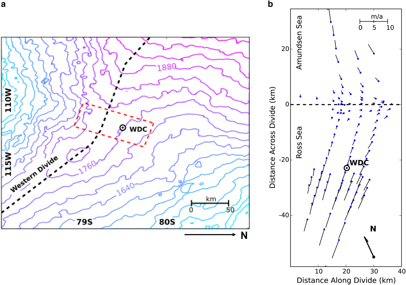
The WAIS Divide ice core site is located in the Ross drainage basin, 24 km downstream of the boundary with the Amundsen basin (Morse and others, Reference Morse, Blankenship, Waddington and Neumann2002). This boundary shows a topographic saddle between higher ice surfaces at the Executive Committee Range and at another ice dome that divides Weddell and Ross/Amundsen drainage basins (Fig. 7a). The surrounding ice lies in a regime of laterally convergent flow – extending across the divide and compressing along it. The Divide is migrating at ~10 m a–1 (Conway and Rasmussen, Reference Conway and Rasmussen2009), but the strain configuration and ice topography have not changed substantially in the last several thousand years (Matsuoka and others, Reference Matsuoka, Power, Fujita and Raymond2012). Some properties for the borehole are listed in Table 2.
(a) Topography of the WAIS Divide near the WAIS Divide Ice Core (WDC) site. Elevation data are from Liu and others (Reference Liu, Jezek, Li and Zhao2001). The GPS survey area for (b) is outlined in red. The contour interval is 40 m. (b) Surface velocities near the WAIS-Divide core site. Divide is at 0 km on vertical axis. Data from Conway and Rasmussen (Reference Conway and Rasmussen2009).
Properties of the WAIS-D Borehole.

* Inclination measured in degrees from vertical.
† Data from Slawny and others (Reference Slawny2014).
Surface velocities at the WAIS Divide were measured by Conway and Rasmussen (Reference Conway and Rasmussen2009). Strain rates at various sites around the divide were calculated with a vector polynomial fit to this data (Conway and Rasmussen, Reference Conway and Rasmussen2009), and from strain nets around individual sites (Matsuoka and others, Reference Matsuoka, Power, Fujita and Raymond2012). We infer typical values for extension and compression in this region with a vector polynomial fit to the surface velocity data (Appendix B) using a modified version of the strategy employed by Conway and Rasmussen (Reference Conway and Rasmussen2009). We force the fitted polynomial to assume spatially independent values (zeroth order) for divergence and curl. Strain rates in the core vicinity are derived by differentiating this flow field.
A depth/age relationship for ice within the WAIS-D core was derived by the WAIS Community Members (2013). Assuming steady state, the rate of vertical compression can be estimated from this relationship by differentiating in time and then depth:  ${\dot \epsilon} _{zz} = (\partial /\partial z)\,(\partial z/\partial t)$ where z is the depth and t is the age in years. We obtain an average value by fitting a first-order polynomial to the depth profile of the time derivative, ∂z/∂t. The slope of this polynomial is a representative value for vertical compression: ${\dot \epsilon} _{zz} $. These findings are summarized in Table 3.
Strain Rates averaged throughout depth in the vicinity of the WAIS Divide. x, y and z are respectively, the along-divide, across-divide and vertical directions.
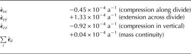
Our results show extension across the divide of magnitude greater than the rate of vertical compression, accompanying substantial compression along the divide. For mass continuity:  ${\dot \epsilon} _{xx} + {\dot \epsilon} _{yy} + {\dot \epsilon} _{zz} = 0$, which is consistent with the values in Table 3.
Uniform horizontal extension is characterized by the strain relationship  ${\dot \epsilon} _{xx} = {\dot \epsilon} _{yy} = - {\dot \epsilon} _{zz} /2$. Pure uniaxial extension across a divide, in contrast, has the strain relationship ${\dot \epsilon} _{xx} = {\dot \epsilon} _{zz} = - {\dot \epsilon} _{yy} /2$. The WAIS Divide strain configuration, shown in Table 3, is closer to the case for horizontal uniaxial extension; this favors the development of vertical-girdle fabrics (Alley, Reference Alley1988).
5.2. Sonic logs
We conducted several sonic logs throughout the depth of the WAIS-D borehole during the 2011/12 season (Data available at http://nsidc.org/data/nsidc-0592). Raw P-velocities inferred from our logs are shown in Figure 8a. Measurements in the upper 2000 m of ice are pervaded by noise that precludes detailed interpretation. All of our logs were performed with a damaged transmitter that likely produced an azimuthally asymmetric signal (The transmitter is a ring-shaped piezo-electric crystal. One section of this ring (~20% of its area) was pulverized on arrival at WAIS. The rest of the transmitter appeared to be intact). This, coupled with poor tool-centralization within the borehole, is the most likely explanation for abrupt upward shifts in inferred P-velocity (typically spanning of the order of 10 m in depth) that are not consistent between logs.
P-wave velocities measured in the WAIS-D borehole. Separate logs are distinguished by color. (a) Raw measurements. (b) 3 m running mean for P-wave velocities from each log. The logs were truncated above 2000 m and were processed to remove large errors associated with physical receiver drift. (c) A close-up comparison of four separate logs near the bottom of the borehole. Separate logs consistently show small (several m s–1) velocity features that occur over short (several meters) depth ranges, but differ systematically by up to 40 m s–1.
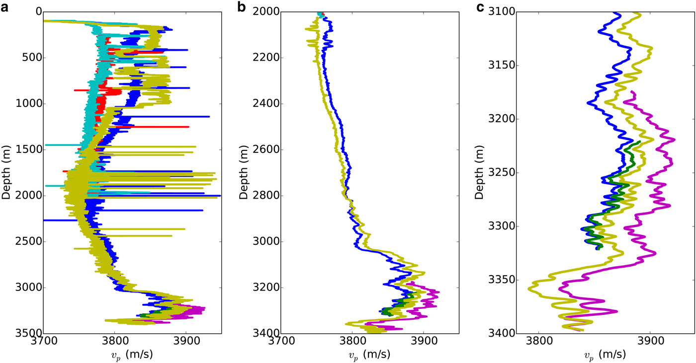
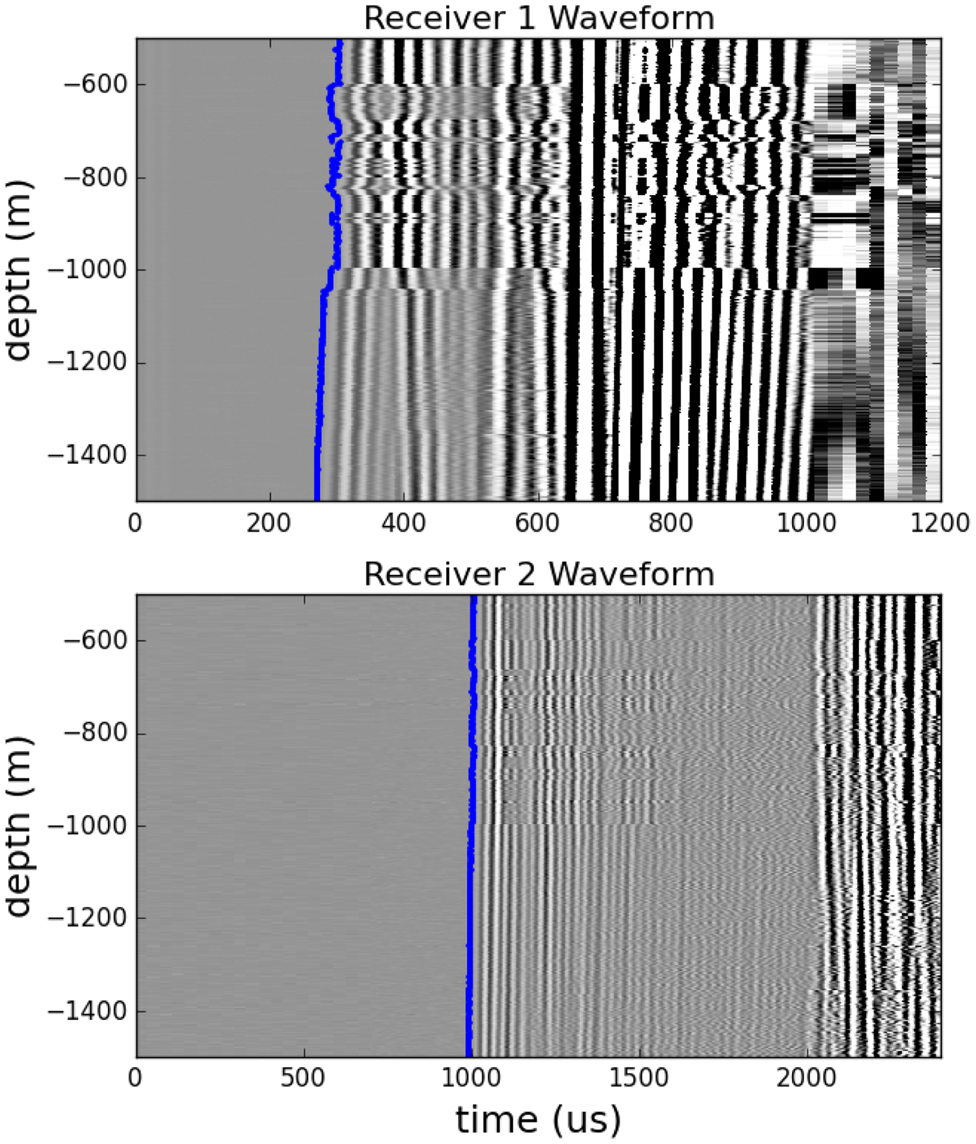
Figure. 9 shows waveforms and measured arrival times for one of our logs. In the upper 1000 m of this log, there are substantial variations in Rx1 arrival times that have no visible counterparts in the Rx2 arrivals. Following from the wave-travel geometry (4L 1 ≃ [L 1 + L 2]), arrival time variations due to ice fabric should be exaggerated in the second receiver by about a factor of 4 (i.e. if the tool enters a fast layer where the Rx1 arrival occurs 2 µs earlier than the local norm, then the Rx2 arrival should occur  $ \approx 8{\kern 1pt} \,{\rm \mu s}$ earlier). The behavior in Figure 9 is not consistent with this rule, and could be explained by Rx1 moving back and forth across the borehole central-axis.
Waveforms measured in the WAIS-Divide borehole. Shades correspond to pressure amplitudes. Calculated arrival times are marked in blue. This particular log is the same as for the dark-blue profile in Figure 8.
There are also persistent differences between logs in the upper 1500 m of ice. This was most likely caused by changes in the tool-centralizer diameter – an unfortunate problem that we were able to partially address for our later logs.
For reasons that are not entirely clear, our measurements have far less noise below 2200 m depth. This improvement could result from greater off-vertical deviation for the borehole axis at greater depths – the tool would have rested more consistently on the down-hole side of a more inclined borehole. Measurements of borehole inclination are consistent with this interpretation; the inclination increases substantially between 1000 and 2000 m depth, and then remains constant. It is also possible that the tool isolators straightened because of warmer ice and borehole fluid at greater depths.
Figure 8b shows 3 m running averages for each log below 2000 m depth. We discard data from shallower depths where data quality was particularly poor. Each log was processed to remove artificial features – we removed major outliers, as well as spikes where the relative behavior of arrival times at Rx1 and Rx2 were not consistent (as described above). Some undesirable artifacts remain, including distinctly opposing velocity features between 2000 and 2200 m in the blue and yellow-green profiles. Presumably, some features in the borehole at these depths caused tool behavior with opposite results for two logs. This behavior underlies the need for precise tool centralization, as well as redundant logs to verify features.
Below 2200 m depth, the noise level decreases substantially, and we see good agreement between features on separate logs. A close-up view of data near the bottom of the ice sheet is shown in Figure 8c. Small velocity features of several m s–1 that occur over short depth ranges (several m) are repeated among separate logs. Although velocities differ systematically between logs by up to 40 m s–1, small-scale features are very consistent between logs (i.e. the results of different logs differ primarily by translation). The most likely explanation for this systematic error is that the distance between receivers and the borehole wall was not consistent between logs. This problem was not a surprise – the tool centralizers were too small for the WAIS-D borehole and were prone to changing diameter – but could easily be corrected for future logs. See the section on error analysis for a quantitative treatment of this effect.
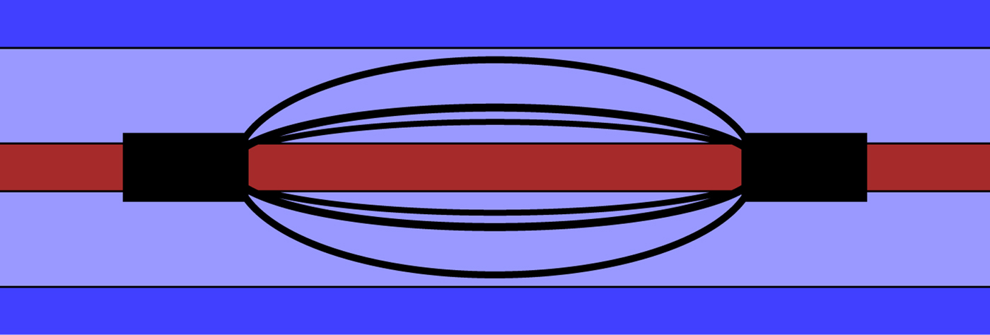
A schematic for a (bow-spring) centralizer that we used at the WIAS Divide is shown in Figure 10. We tried to control the diameter of the centralizers by adjusting the distance between cuffs – this was ineffective because the cuffs would slide apart during logs until the centralizer diameter was barely greater than that of the tool. For subsequent logs (at the North Greenland Eemian Ice Drilling (NEEM) core), we were able to control the distance between cuffs by connecting them under tension with a steel rod. We recommend that future sonic loggers do the same.
Bow-spring centralizers can keep a tool in the center of a borehole. Flexible rods bow out between two cuffs. For our logs at the WAIS Divide, we did not have an effective way to control the centralizer radius. One way to control centralizer radius is by adjusting the distance between cuffs with a steel rod that connects them under tension (not shown). This method has worked well in subsequent logs.
5.3. Thin sections
Using optical methods, Voigt and colleagues measured crystal fabrics (Data available at http://nsidc.org/data/nsidc-0605) on ~10 cm × 10 cm thin sections that were cut vertically from the WAIS-D core at 83 depths (average separation of ~40 m vertical between measurements). Fitzpatrick and others (Reference Fitzpatrick2014) provided an area and two orientation angles for each thin section. This provides a detailed description of ice fabric at a discrete set of depths. From each fabric measurement, we can calculate a corresponding eigenvalue set with (1) or a corresponding vertical P-wave velocity with (4) and (7).
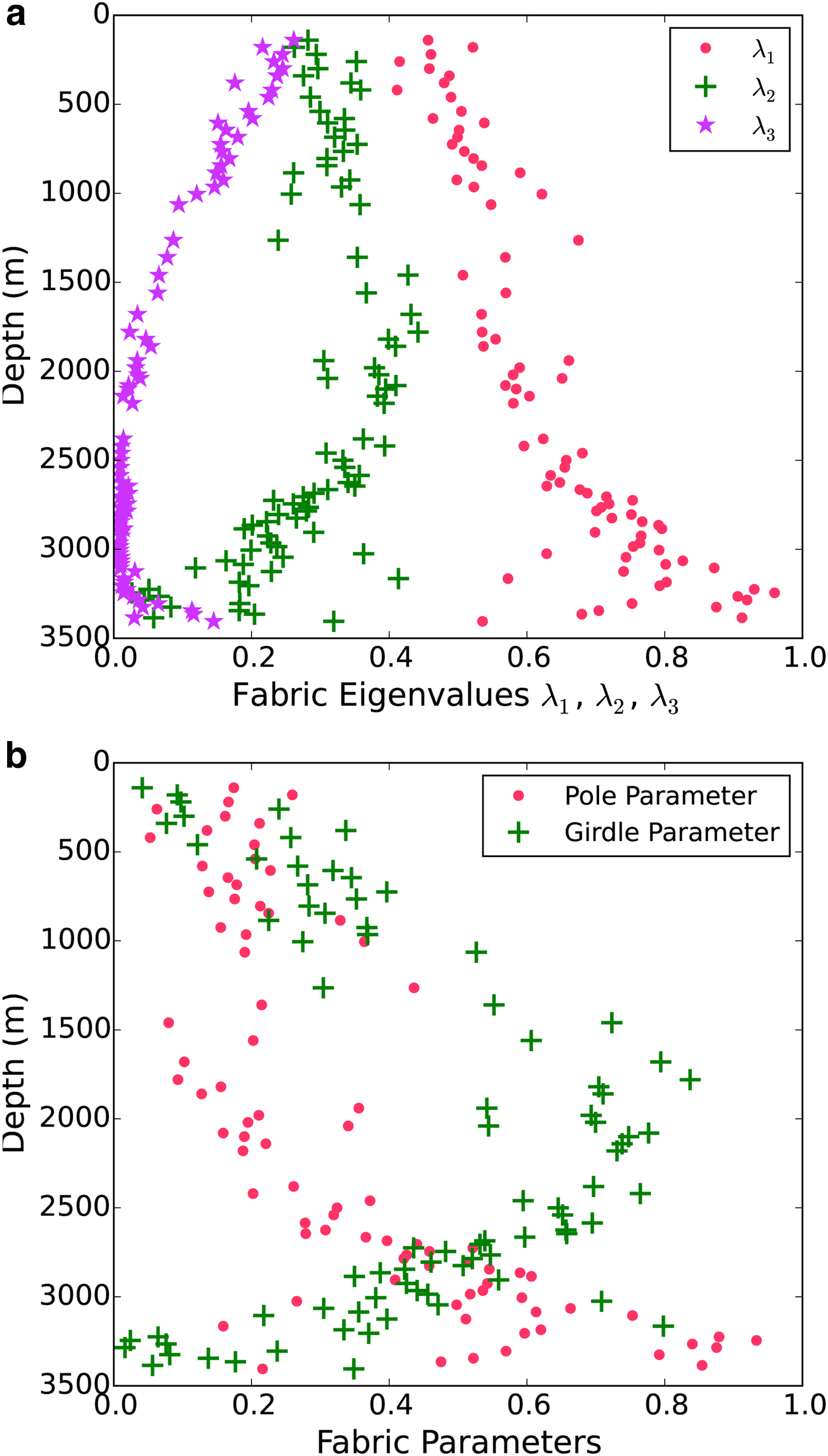
Fabric eigenvalues for all thin-section measurements are shown in Figure 11a. Fabric parameters, as a function of ice depth, are shown in Figure 11b. At the WAIS Divide, fabric gradually develops into strong girdles in the upper 2000 m of ice. Below 2000 m, there is a relatively abrupt shift to vertical-pole fabrics, until the bottom several hundred meters, where the pole parameter varies substantially between measurements and has a lower average magnitude.
Depth variation of COF characteristics inferred from thin sections. (a) Fabric eigenvalues (Section 2.1). (b) Pole and girdle parameters derived from eigenvalues.
5.4. Prevailing fabrics at the WAIS divide
Strain evolution causes ice-crystal c-axes to align in directions of compression. As a consequence, vertical-pole fabrics are favored in ice where vertical compression accompanies approximately uniform extension in the horizontal. This is the case at ice domes and ridges with no lateral convergence (Dome C and NEEM, respectively). At the WAIS Divide, in contrast, horizontal ice flow convergence that is transverse to the flow direction produces a compression rate (along one horizontal axis) of magnitude sufficiently close to the vertical compression rate for c-axes to distribute throughout a vertical plane – they form vertical girdles that include both the vertical and horizontal axes of compression. The prevalence of these girdles in the upper 2500 m of ice is demonstrated by thin-section measurements (Fig. 11), and is consistent with, but not readily inferred from, the existing sonic data. Radar measurements at the core site show polarimetric features that can be caused by vertical-girdle fabrics at depths <1800 m (Matsuoka and others, Reference Matsuoka, Power, Fujita and Raymond2012); below 1800 m the signals are too small to see such features. Below 2500 m depth there is a transition to pole fabrics, which our sonic logs record in detail.
6. DISCUSSION
6.1. P-wave interpretation
6.1.1. Resolution and accuracy
Our tool measures elastic waves that travel a distance of 3 m between receivers. Velocity features that are repeated among separate logs occur over depth ranges of this magnitude (Fig. 8c). These same features have velocity magnitudes as low as 1 m s–1. Based on the repeatability of these measurements, we report that our tool can resolve relative velocity differences on the order of 1 m s–1 with a depth resolution of 3 m.
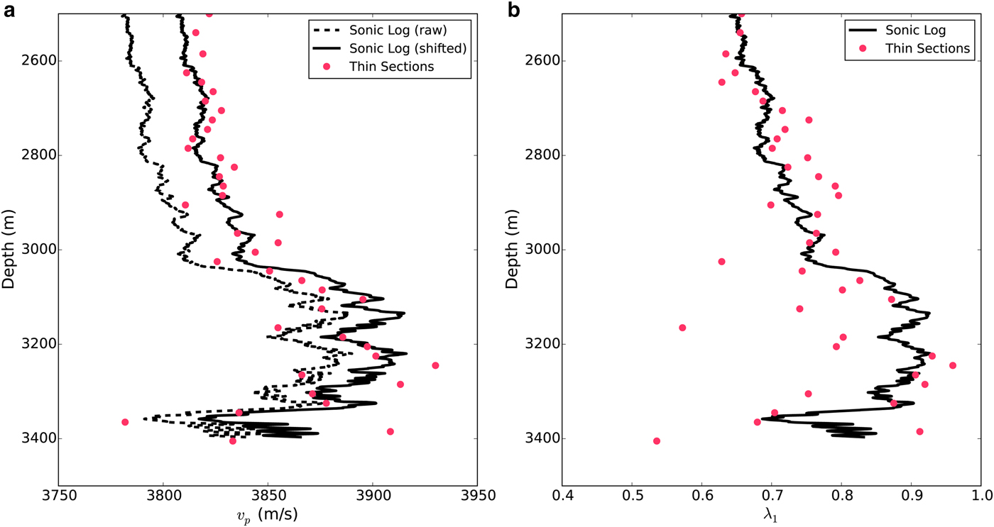
Consistent separation between redundant logs demonstrates substantial systematic error in our data, with up to 40 m s–1 separation between measurements at the same depth (in regions where noise was low). Because of this systematic bias, raw velocity profiles inferred from our data should be assumed to be offset from correct velocities, with biases on the order of 10 m s–1. One way to reduce this bias is to shift the measured velocity profiles so that they coincide with theoretical velocity profiles based on thin-section measurements. We employ this method below to infer fabric parameters from the sonic data. Ideally, future surveys will reduce this problem with a well-centralized tool.
6.1.2. Relationship to fabric – λ 1 (v p)
The speed of a vertically propagating P-wave is related to vertical clustering of ice-crystal c-axes. Figure 12 compares eigenvalue-based fabric parameters to predicted (using 4 and 7) wave velocities for both thin-section and idealized synthetic fabric distributions. Figures 12a, b show predicted velocities for a fabric based on its pole parameter and first eigenvalue, respectively. In each case, the idealized fabrics are a set of pole-type Fisherian distributions. In Figure 12b, the relationship for girdle-type Fisherian distributions is also shown – this cannot be done for Figure 12a because all girdle-type Fisherian distributions have a pole parameter of zero, regardless of fabric strength.
Comparison of COF features and predicted (using 4 and 7) wave speeds for both measured thin-section fabrics (dots) and for idealized Fisher-distribution (dashed lines) fabrics. (a) shows the relationship between pole parameter λ 1 − λ 2 and P-wave speed v p. (b) shows P-wave speed v p as a function of the largest eigenvalue λ 1. This relationship is also shown for the Fisher girdle distributions, although their range on the λ 1 axis is narrow. (c) shows how the speeds of fast- and slow-polarized shear waves are affected by girdle development for observed fabrics and synthetic girdles. (d) shows the separation between fast and slow shear waves for the same fabrics as in (c).
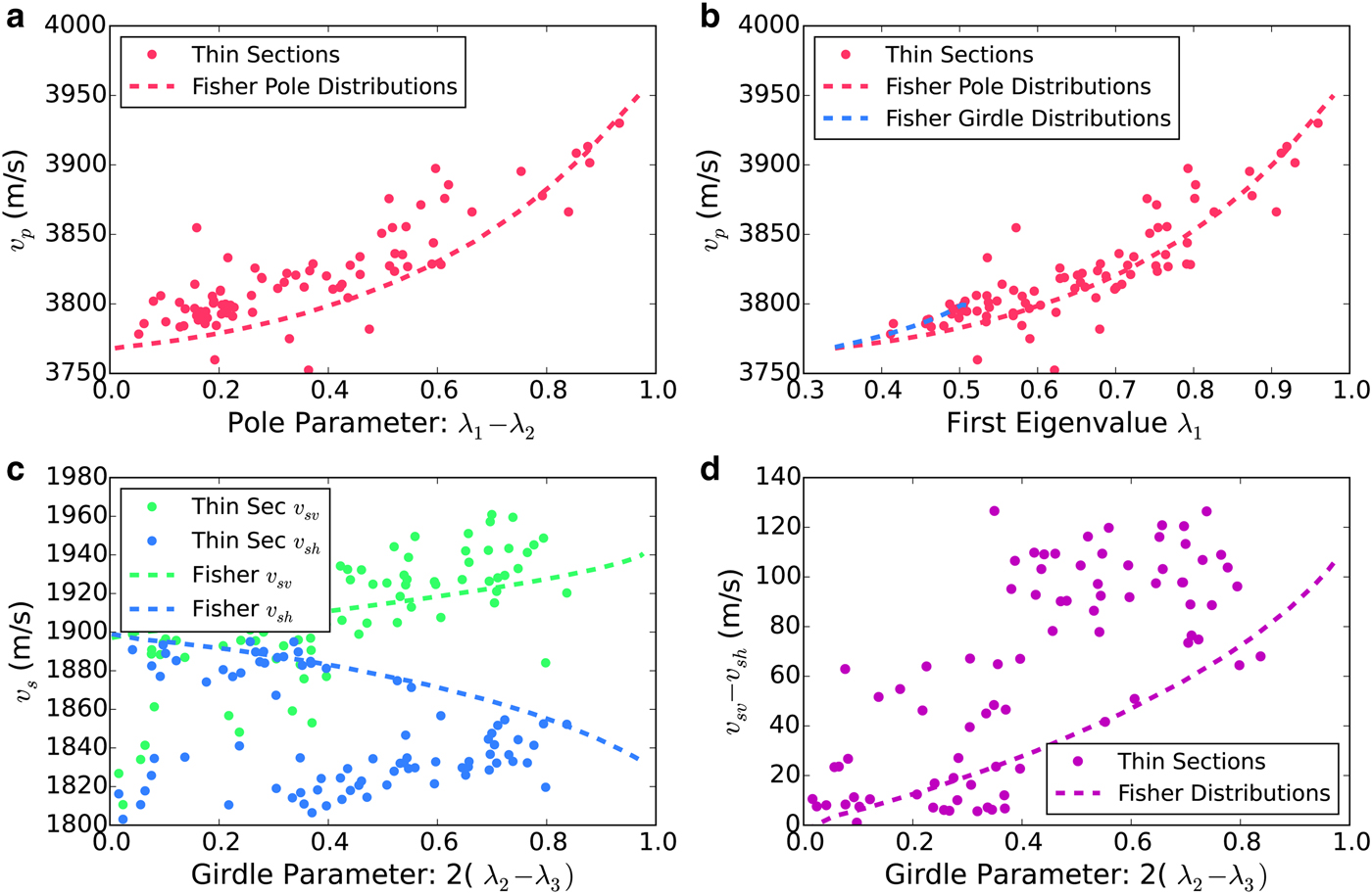
P-wave velocity is sensitive to a fabric's pole parameter, as well as its first eigenvalue, λ 1. Figure 12b shows that the relationship between v p and λ 1 is similar for a variety of fabrics – girdle- and pole-type Fisherian distributions, as well as fabrics measured at the WAIS Divide. This observation justifies using v p as a proxy for the first eigenvalue of the fabric of the measured ice. The v p(λ 1) relation for pole-type Fisherian distributions is one-to-one, as well as a good representation of the relation for thin-section fabrics. By taking the inverse of this relationship, measured P-wave velocities can be converted to fabric eigenvalues λ 1.
Figure 13 shows the results of this λ 1(v p) function applied to P-wave speeds (average of multiple logs) that we measured at the WAIS Divide. Before solving for λ 1 (Fig. 13b), we shifted the velocity profile (Fig. 13a) to minimize the first-order mismatch between measured velocities and thin-section predicted velocities at corresponding depths below 2500 m. The sonic-derived eigenvalues agree well with thin-section measurements in the low-noise region below 2500 m. There is a region ~3100 m depth where the thin-section λ 1s are consistently lower than the sonic-derived values. This disagreement is not present in the relationship between velocity measurements and thin-section predictions (Fig. 13a), and reflects the imperfect (but generally very good) relationship between velocities and eigenvalues. Because sonic data quality was poor in the upper ice, we draw no conclusions about fabric from our sonic logs above 2500 m.
Fabric parameter λ 1 inferred from P-wave velocities, compared with thin-section values. (a) Measured P-wave velocities compared to theoretical predictions (using (4) and (7)) from thin-section data at corresponding depths. Raw velocities (dashed line) were shifted (solid line) to minimize the first-order misfit with corresponding thin-section values. (b) Fabric eigenvalues λ 1 inferred from wave velocities, compared with those calculated from thin sections. Eigenvalues are inferred from P-wave velocities using the red curve in Figure 12b.
Gusmeroli and others (Reference Gusmeroli, Pettit, Kennedy and Ritz2012) suggested a similar relationship between v p and λ 1 that was interpolated from a direct comparison of thin-section-derived eigenvalues to elastic wave speeds measured with the same CLP-4877 tool. Because of systematic bias inherent in this tool, we advocate interpreting measured wave-speeds as possible offsets from true values, rather than as absolute values. We avoid this problem by employing a v p(λ 1) relationship based on theoretical values for measured fabrics, and using it to calibrate our measured velocities so they coincide with thin-section data.
The relationship between v p and λ 1 relies on the eigenvector associated with λ 1 being aligned near the vertical. This is consistently the case for thin-section measured fabrics at the WAIS Divide. The relationship would break down for pole fabrics that are not aligned with the vertical, such as may be present in regions of stratigraphic folding. The general interpretation – that fast P-wave speeds correspond to clustering of c-axes in the vertical – would still be true.
6.2. S-Wave interpretation – next step for sonic logging
P-wave velocities are not sensitive to azimuthal clustering of ice-crystal c-axes, as is present in vertical-girdle fabrics. This can be seen in Figures 3 and 12b (Note that in Fig. 12b, vertical girdles occur only within a small subset of the plotted domain. Although v p varies rapidly with λ 1, its total range is small because λ 1 for vertical-girdle fabrics is restricted to the narrow range between 0.33 and 0.5). First-arriving shear waves are respectively, faster and slower for strong girdle and pole fabrics, and may be useful for distinguishing between the two. As a fabric develops from isotropic to a strong girdle, v sv increases by ~2%, which would be difficult, but not necessarily impossible to detect with sonic methods. Another sonic feature of vertical-girdle fabrics is shear-wave splitting into fast and slow polarizations (v sv and v sh) that are respectively, parallel and normal to the girdle plane. For a strong girdle, the difference between these two velocities is ~100 m s–1 (5%).
Shear-wave splitting is strongly related to girdle strength for both synthetic and observed fabrics. Figure 12c shows the relationship between girdle parameter and shear-wave velocities for observed (thin section) and synthetic (Fisherian girdle) distributions. Points in the bottom left that appear at odds with the Fisherian-distribution relationships correspond to vertical-pole fabrics, which have low girdle parameters and low speeds for both shear-wave types. Because it is hard to distinguish corresponding pairs of v sv and v sh, we plot the difference v sv – v sh in Figure 12d. A clear relationship between girdle strength and velocity splitting is evident for both observed and synthetic distributions. Notably, the girdle model for azimuthally-anisotropic fabrics is an imperfect representation of the actual fabrics that exist at the WAIS divide, and this is reflected in disagreement between the real-fabric and idealized distribution shear-splitting predictions. Nevertheless, thin-section fabrics demonstrate a correlation between shear-wave splitting and girdle strength that can be used to infer girdle strength from shear-wave splitting in a probabilistic sense. Alternatively, one could use shear-wave splitting on its own as a proxy for azimuthal anisotropy.
The data we collected at the WAIS Divide are of insufficient quality to accurately distinguish S-wave arrivals. This was in part due to clipping of the high-amplitude S-wave signals that precludes most forms of signal processing. Receivers with greater dynamic range could better record both P- and S-wave arrivals. Because S waves are slower than P waves, their arrivals are obscured by any remnant energy in the P-wave coda – even without amplitude clipping, S-wave arrivals cannot be picked with the same resolution as P-wave arrivals. Shear-wave speeds can also be measured by optimizing a correlation coefficient across the S-wave regions of multiple waveforms. This method, known as semblance analysis, is common in borehole logging (e.g. Luo and Hale, Reference Luo and Hale2012). We are working with a contractor to build a new tool with improved dynamic range to simultaneously resolve both P- and S-waves. This tool will feature five receivers that are equally spaced over a vertical span of 3 m, allowing us to resolve S V velocities with semblance analysis.
Ideally, future loggers will be able to detect both v sv and v sh arrivals. An industry precedent for detecting separate shear-wave velocities uses a combination of flexural-wave logging (Haldorsen and others, Reference Haldorsen2006) and semblance analysis (Luo and Hale, Reference Luo and Hale2012). Flexural-wave logging requires a low-frequency (order kHz) tool that is not well suited to P-wave logging, so we have focused on measuring P and S head-waves in our ongoing tool development.
6.3. Method comparison
Fabric can be expected to vary on long spatial scales (meters to hundreds of meters) due to general bulk strain, and on short spatial scales (centimeters to meters) due to local differences in grain/scale interactions and recrystallization, as well as to seasonal and annual differences in impurity loading in snowfall. In principle, thin sections can resolve sub-meter fabric properties, if thin sections can be obtained continuously along the length of a core. However, in practice, thin sections have not been obtained continuously along the length of any major ice core, and the distance between nearby thin sections has typically been tens of meters. For example, at WAIS Divide, thin-section measurements were taken at an average interval of 40 m.
In our study, sonic logs, which average fabric over 3 m depth, show relatively minor deviations from a local trend over distances of 100 m or more, suggesting that fabric varies relatively smoothly on wavelengths greater than a few meters. In contrast, individual thin sections capture local fabric on the decimeter scale at isolated points in a core, and the wide scatter of thin-section results in Figure 13b (relative to the sonic results) implies that there are large variations in fabric on some spatial scale that is significantly shorter than 3 m.
Neither sonic nor thin-section data from the WAIS Divide can resolve these meter-scale variations. Sonic measurements average out fabric properties at the meter scale, and therefore are unable to resolve any features at or less than that scale. With available thin sections, meter-scale variations are irretrievably aliased, due to the typically large depth separations between thin sections.
Our sonic data from the WAIS Divide do detect small fabric changes (variations in λ 1 that are much smaller than 0.1 in Fig. 13b) over depth spans of a few meters and greater. Notably, this is the smallest scale of interest for ice-sheet modeling, for which model mesh size is a constraint. These same features cannot be resolved at all with the thin sections that are available from the WAIS divide. In order to resolve fabric variability occurring over depth ranges of a few meters, the depth interval between thin sections would need to be reduced to a few decimeters, i.e. by one to two orders of magnitude.
Automated fabric analyzers (e.g. Wilen, Reference Wilen2000) have reduced the labor requirements for thin-section measurements and may allow for much smaller separations between thin sections in future cores. At the same time, thin-section measurements consume core, and a generous allotment of ice would likely be necessary to greatly increase the number of thin-section samples. Given the small number of grains in each thin section, particularly at depths where grains have grown substantially, it could take multiple samples per meter of core to convincingly detect the fabric variations over several meters to which a sonic tool is sensitive. Given this constraint, we anticipate that for the foreseeable future sonic logging will be the most effective means to detect fabric changes that occur over depth ranges of a few meters.
7. CONCLUSIONS
By measuring the velocities of vertically-propagating P waves in a borehole, we are able to infer the vertical clustering of ice crystal c-axes, including abrupt variations that occur in the lower ice at the WAIS Divide. The velocity that we measure is closely related to the fabric eigenvalue λ 1. We measure λ 1 continuously in depth, and are able to resolve small ( ≪ 0.1) changes that occur over several meters of depth. These features cannot be inferred from available thin sections, and could not be detected with thin sections without a great increase in the thin-section sampling rate.
We recommend inferring eigenvalues from P-wave velocities as follows:
(1) Shift measured velocities to minimize disagreement with theoretical values based on thin-section measurements, as in Figure 13a.
(2) Use the red curve in Figure 12b. to convert adjusted velocities to values for λ 1.
Better tool centralization will minimize systematic bias in raw wave speeds, but the strong sensitivity of sonic measurements to receiver position probably necessitates some calibration with direct fabric measurements (step 1) for future logs.
Current methods for sonic logging can also be improved with additional tool receivers that allow for semblance analysis. P-wave measurements are appropriate for distinguishing vertical-pole from isotropic fabrics; they are insensitive to girdle-fabrics. In the future, by measuring both P- and S-wave arrivals, as well as the separation between fast and slow shear polarizations, it will be possible to further distinguish girdle fabrics around an ice borehole. This will be especially useful for logging at sites like the WAIS Divide where ice flow converges along a horizontal axis.
ACKNOWLEDGEMENTS
This work was supported by a National Science Foundation Graduate Research Fellowship to Dan Kluskiewicz and under NSF grants PLR-0944199, PLR-0944285, and PLR-0539578. Ryan Bay, Gary Clow, Elizabeth Morton, and Frank Urban assisted with the sonic-log measurements. The authors appreciate the support of the WAIS Divide Science Coordination Office at the Desert Research Institute, Reno, NE, USA and University of New Hampshire, USA, for the collection and distribution of the WAIS Divide ice core and related tasks (NSF Grants 0230396, 0440817, 0944348; and 0944266), and Kristina Slawny for providing the borehole inclination data. Kendrick Taylor led the field effort that collected the samples. The National Science Foundation Division of Polar Programs also funded the Ice Drilling Program Office (IDPO) and Ice Drilling Design and Operations (IDDO) group for coring activities; the National Ice Core Laboratory for curation of the core; the Antarctic Support Contractor for logistics support in Antarctica; and the 109th New York Air National Guard for airlift in Antarctica. We also appreciate input from Mike Hay, Erin Pettit and Alessio Gusmeroli, as well as extensive advice and tool service support from John Stowell at Mt. Sopris Instruments Inc.
APPENDIX A
FRESNEL ZONE CALCULATION
We approximate the first Fresnel zone as an elongated toroidal object with a half cross section as is depicted in the red region of Figure 14. This cross section is half of an ellipse with semi-major axis b and semi-minor axis a. From the definition of the first Fresnel zone, it follows that b = L/2 + λ/4 and a 2 + (L/2)2 = b 2. The solution for a is
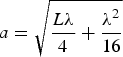 $$a = \sqrt {\displaystyle{{L\lambda} \over 4} + \displaystyle{{\lambda ^2} \over {16}}} $$
A cross section of the Fresnel volume for sampled ice is shown in red. It is half of an ellipse with semi-major axis b and semi-minor axis a. The volume was calculated by rotating the cross section about the borehole central axis.
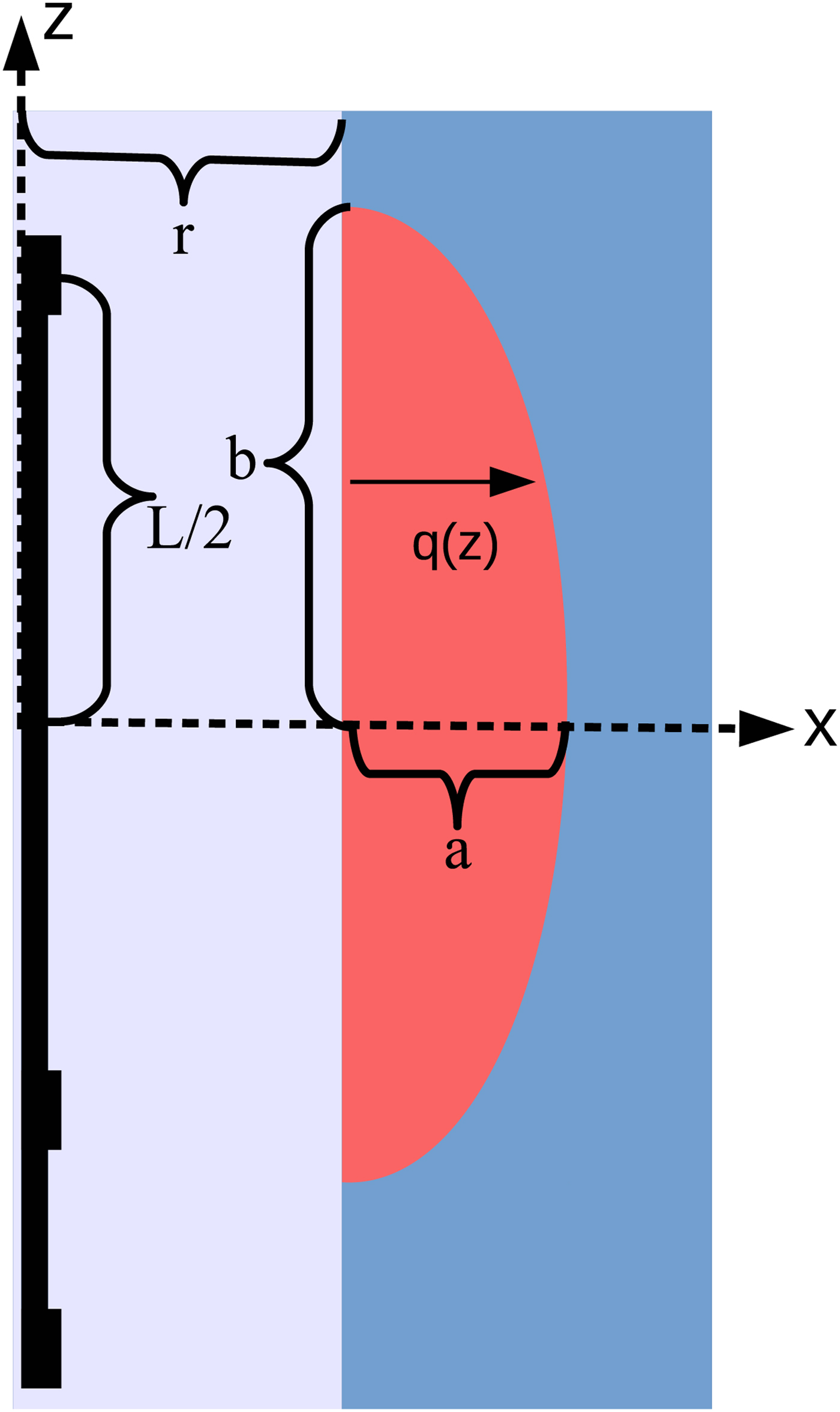
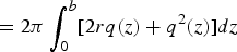
Let q(z) be the radial distance from the borehole wall to the edge of the Fresnel zone at a given depth z. The Fresnel volume can be found with an integral along the z-axis:
 $$V = 2\vint_0^b \pi [(r + q(z))^2 - r^2 ]dz$$
 $$= 2\pi \vint_0^b [2rq(z) + q^2 (z)]dz$$
 $$= 2\pi rA_{\rm e} + V_{\rm e} $$
where A e and V e are the area and volume for an ellipse with semi-minor and semi-major axes a and b. Then A e = πab, V e = 4πa 2 b/3 and
 $$V = \pi ab(4a/3 + 2\pi r) $$
FITTING A FLUX FIELD
Given vectors  ${\bf u(x},{\bf y)}$ and ${\bf v(x},{\bf y)}$ describing velocity components on coordinate vectors x and y (e.g. u 1 is the along-divide surface velocity at point (x 1, y 1), see Fig. 7b), the local horizontal ice flux is
 $$\left( {\matrix{ {{\bf q}_{\bf x} {\bf (x},{\bf y)}} \cr {{\bf q}_{\bf y} {\bf (x},{\bf y)}} \cr}} \right) = {\bf h(x},{\bf y)}\, {\scriptscriptstyle\circ} \,{\bf g(x},{\bf y)} \,{\scriptscriptstyle\circ} \,\left( {\matrix{ {{\bf u(x},{\bf y)}} \cr {{\bf v(x},{\bf y)}} \cr}} \right)$$
where h is the measured height corresponding to points in x and y, γ is a scale factor that converts surface velocity to the depth-averaged velocity and ° indicates element-wise multiplication. Values for u, v, x, y, h and γ are taken from Conway and Rasmussen (Reference Conway and Rasmussen2009).
A vector polynomial can be fitted to the ice fluxes with arbitrary limits on the polynomial order for divergence and curl. Let N be the number of measurement points and P be the desired order for the flux polynomial. The vector polynomial can take the form
 $$\left( {\matrix{ {q_x (x,y)} \cr {q_y (x,y)} \cr}} \right) = \sum\limits_{k = 0}^P \sum\limits_{i = 0}^k \left( {\matrix{ {\alpha _{i,k - i}} \cr {\beta _{i,k - i}} \cr}} \right)x^i y^{k - i} $$
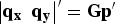
Over the domain x and y, this relationship takes the form
 $$\left \vert {{\bf q}_{\bf x} \;\;{\bf q}_{\bf y}} \right \vert ^{\prime} = {\bf Gp}^{\prime} $$
where
 $${\bf p} = \left \vert {\alpha _{0,0} \;\;\alpha _{1,0} \;\;\alpha _{0,1} \;\;...\;\;\alpha _{0,P} \;\;\beta _{0,0} \;\;\beta _{1,0} \;\;\beta _{0,1} \;\;...\;\;\beta _{0,P}} \right \vert $$
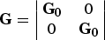
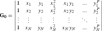
G is the coordinate matrix
 $${\bf G} = \left \vert {\matrix{ {{\bf G}_{\bf 0}} & 0 \cr 0 & {{\bf G}_{\bf 0}} \cr}} \right \vert $$
and
 $${\bf G}_{\bf 0} = \left \vert {\matrix{ 1 & {x_1} & {y_1} & {x_1^2} & {x_1 y_1} & {...} & {y_1^P} \cr 1 & {x_2} & {y_2} & {x_2^2} & {x_2 y_2} & {...} & {y_2^P} \cr \vdots & \vdots & \vdots & \vdots & \vdots & \ddots & \vdots \cr 1 & {x_N} & {y_N} & {x_N^2} & {x_N y_N} & {...} & {y_N^P} \cr}} \right \vert $$
(B8) can be solved for p without any constraints on the divergence and curl. To limit the polynomial order for divergence and curl fields to D and C, respectively, it must be that
 $$i\alpha _{i,k - i} + (k - i + 1)\beta _{i - 1,k - i + 1} = 0 $$
for k > D + 1 and 1 ≤ i ≤ k and
 $$i\beta _{i,k - i} - (k - i + 1)\beta _{i - 1,k - i + 1} = 0 $$
for k > C + 1 and 1 ≤ i ≤ k
This can be accomplished by solving
 $$[{\bf G} + \eta {\bf L}]{\kern 1pt} {\bf p^{\prime}} = \left \vert {{\bf q}_{\bf x} \;\;{\bf q}_{\bf y}} \right \vert ^{\prime} $$
where
 $$\eqalign{& {\bf L}(row,\zeta _{i,k - i} ) = i \cr & {\bf L}(row,\zeta _{i - 1,k - i + 1} + M/2) = k - i + 1} $$
for D <k ≤ P and 1 ≤ i ≤ k and
 $$\eqalign{& {\bf L}(row,\zeta _{i,k - i} + M/2) = i \cr & {\bf L}(row,\zeta _{i - 1,k - i + 1} ) = k - i + 1} $$
for C < k ≤ P and 1 ≤ i ≤ k
ζ i,j is the index of α i,j in p and M is the number of columns in G. ‘row’ is increased iteratively with each assignment, starting from 1. η is a trade-off parameter between the least-squares fit and the polynomial order constraints – a large value strictly constrains the divergence- and curl-field orders.
This method is readily implemented with any linear algebra programming package that can calculate a matrix pseudo-inverse, including matlab and numpy.


 Open access

