

1. INTRODUCTION
Himalayan glaciers play a crucial role in regional water resources (Immerzeel and others, Reference Immerzeel, Van Beek and Bierkens2010) and are also considered to be a climate indicator in high-altitude and mid-latitude regions (Gardelle and others, Reference Gardelle, Berthier, Arnaud and Kääb2013), although the response of debris-covered glaciers to climate change is poorly understood (Scherler and others, Reference Scherler, Bookhagen and Strecker2011). In the Himalayas, glaciers have experienced generally negative trends in mass (Gardner and others, Reference Gardner2013), area (Cogley, Reference Cogley2016) and terminus position (Bolch and others, Reference Bolch2012), with glacier shrinkage exhibiting high-spatial variability (Fujita and Nuimura, Reference Fujita and Nuimura2011; Yao and others, Reference Yao2012; Gardelle and others, Reference Gardelle, Berthier, Arnaud and Kääb2013; Kääb and others, Reference Kääb, Treichler, Nuth and Berthier2015). The continuous shrinkage of these glaciers during the past couple of decades has drawn serious attention from the scientific community, local authorities and other concerned stakeholders (Cogley and others, Reference Cogley, Kargel, Kaser and Van der Veen2010). However, uncertainty remains high because of the scarcity of high-quality data owing to spatial and temporal resolution, inconsistent methods of measurement, poor visibility due to snow and cloud cover, and unclear extent of debris-covered portions (Paul and others, Reference Paul2013; Cogley, Reference Cogley2016).
The Khumbu region in eastern Nepal Himalaya, with a large glacier extent at high altitude, has been investigated in terms of glacier area and volume changes, and its glaciers have shown substantial shrinkage during the past couple of decades (Bolch and others, Reference Bolch, Buchroithner, Pieczonka and Kunert2008, Reference Bolch, Pieczonka and Benn2011; Nuimura and others, Reference Nuimura, Fujita, Yamaguchi and Sharma2012; Shangguan and others, Reference Shangguan2014; Thakuri and others, Reference Thakuri2014). For instance, Thakuri and others (Reference Thakuri2014) investigated 400 km2 of glaciers in the Khumbu region through the past five decades (1960–2011) and found an area loss of 13.0 ± 3.1%. Similarly, Shangguan and others (Reference Shangguan2014) reported an area loss of 19.0 ± 5.6% in the Koshi Basin during 1976–2000, which was more pronounced on the southern than on the northern flank of the Mount Everest region. On the other hand, apparent mass changes of −0.32 ± 0.08, −0.40 ± 0.25 and −0.16 ± 0.16 m w.e. a−1 were reported in the Khumbu region by Bolch and others (Reference Bolch, Pieczonka and Benn2011), Nuimura and others (Reference Nuimura, Fujita, Yamaguchi and Sharma2012) and Gardelle and others (Reference Gardelle, Berthier, Arnaud and Kääb2013), respectively. Based on an ice-distribution model, Shea and others (Reference Shea, Immerzeel, Wagnon, Vincent and Bajracharya2015) demonstrated moderate volume and area losses of 15 and 20%, respectively, for the Dudh Koshi Basin during the past five decades (1961–2007). On a broader scale, a recent study revealed that 24% of the glacier area in the whole Nepal Himalaya has been lost over the past three decades (1980–2010) (Bajracharya and others, Reference Bajracharya, Maharjan, Shrestha, Bajracharya and Baidya2014a), and an identical value (23.3 ± 0.9%) was also reported in the Bhutan Himalaya for the same period (Bajracharya and others, Reference Bajracharya, Maharjan and Shrestha2014b). The reason for such reports of rapid loss of glaciers may be misinterpretation of snow and debris cover (e.g. Bhambri and Bolch, Reference Bhambri and Bolch2009) as Landsat images (30 m) were used for both of these studies. Previous glacier mapping has been based mainly on satellite imagery of relatively coarse resolution, such as the Landsat images used for the Randolph (Pfeffer and others, Reference Pfeffer2014), the ICIMOD (Bajracharya and others, Reference Bajracharya, Maharjan, Shrestha, Bajracharya and Baidya2014a, Reference Bajracharya, Maharjan and Shresthab) and the GAMDAM (Nuimura and others, Reference Nuimura2015) glacier inventories. Even though the accuracy of glacier delineation is largely independent of the spatial resolution of the dataset (Paul and others, Reference Paul2013), it was not possible to quantify completely disappeared glaciers, which was one of the goals of this study, with the comparatively coarse resolution of Landsat images. Hence, this study aimed to identify the changes in glacier area in the eastern Nepal Himalaya, from the Kanchenjunga region in the east to the Ganesh Himal region in the west, using high-resolution aerial photographs and remote sensing imagery (<2.5 m) from 1992 to 2006–10. We also examined the dependency of the glacier area change on several topographical parameters.
2. STUDY AREA AND CLIMATE
Nepal, located in the central Himalayas, has 3808 glaciers covering nearly 3902 km2 (Bajracharya and others, Reference Bajracharya, Maharjan, Shrestha, Bajracharya and Baidya2014a). Because of the availability of aerial photographs from 1992, our inventory was confined to the Nepalese territory from the Ganesh region (84°50′E) to the Kanchenjunga region (88°10′E). We defined four major massifs (Ganesh, Langtang, Khumbu and Kanchenjunga) to analyse regional glacier shrinkage (Fig. 1a).

Fig. 1. (a) Glacier distribution from the ALOS glacier inventory for the eastern Nepal Himalaya, in which debris-free (C-type) and debris-covered (D-type) glaciers are distinguished. Background is from the ASTER-GDEM2. (b) Coverage of satellite imagery used in this study (rectangles), tie points to superpose the 1992 onto the ALOS glacier inventory (stars) and disappeared glaciers distribution (open circles). The four massifs are defined by the major river basins.
The climate of eastern Nepal is dominated by the Indian monsoon, which is regarded as a main source for glacier accumulation (Ageta and Higuchi, Reference Ageta and Higuchi1984). The majority of the annual rainfall (>70%) occurs in June–October, and the annual total decreases from east to west and south to northwest (Shrestha and others, Reference Shrestha, Wake, Dibb and Mayewski2000; Bookhagen and Burbank, Reference Bookhagen and Burbank2010). According to energy-mass balance modeling, the glaciers located in a summer precipitation climate tend to be more sensitive to temperature changes than those located within a winter-precipitation climate (Fujita and Ageta, Reference Fujita and Ageta2000; Fujita, Reference Fujita2008). Sakai and others (Reference Sakai2015) also confirmed the higher sensitivity of mass balance to temperature of debris-free glaciers in the summer accumulation region by analysing a wide region of Asia. Although few climate data have been available in the Himalaya so far, Salerno and others (Reference Salerno2015) recently examined the data accumulated over the past two decades (1994–2013) from seven weather stations in the Khumbu region and showed decreasing precipitation (−13.7 ± 2.4 mm a−1; p < 0.001) and increasing minimum temperature (+0.072 ± 0.011°C a−1; p < 0.001).
3. DATA AND METHODS
3.1. 1992 glacier inventory
In November 1992, aerial photographs (coverage of 12 km2 per image) were taken over the eastern Nepal Himalaya by the Survey Department of Nepal, with financial and technical assistance from Finland. Based on these photographs, 1 : 50 000-scale topographic maps (toposheets hereafter) were published by the Survey Department of Nepal. Although the toposheets contained various geographical features, such as forests, wetlands, lakes and glaciers, many seasonal snow surfaces and bright sandy slopes were mistakenly identified as glacier surfaces. To compile a new and updated glacier inventory, one of the co-authors of this study (K. Asahi) performed aerial photograph investigation work for glacier delineation with the aid of a stereoscope at the Department of Hydrology and Meteorology of Nepal between June 1996 and May 1997. A large number of photographs (406) was available and the photographs were well distributed over the region (Kanchenjunga: 139, Khumbu: 196 and Langtang/Ganesh: 71), so the investigator had multiple choices. The main advantage of the stereoscope method for glacier mapping from original aerial photographs is that glaciers can be recognised as 3-D objects, allowing the separation of glacier ice from snow-covered slopes. Similarly, snow-covered ice was also considered and discriminated stereoscopically by analysing its surface features, e.g. an even surface was considered as rock (ice-free), covered with a (thin) snow cover while an uneven (bumpy) surface was interpreted as snow-covered ice. Additionally, the irregular surface of debris-covered glaciers can be identified clearly where there is no dead ice or rock glaciers. The glacier outlines were later delineated on the original toposheets, scanned and re-digitized to reduce distortions pertaining to scanning process, and finally obtained in a polygon shapefile format.
To compare the two glacier inventories used in this study, we needed to cross-examine and validate the 1992 inventory. However, the original aerial photographs could not be used outside Nepal. Therefore, we used Thematic Mapper (TM) images from Landsat 4 and 5 (Table 1), which are freely downloadable from http://glovis.usgs.gov/ (last access: 08 June 2015). The Landsat TM data were used to confirm the presence or absence of disappeared glaciers i.e. those glaciers that were available in the 1992 inventory but completely disappeared in Advanced Land Observing Satellite (ALOS) images. The Landsat images were chosen based on a multitemporal approach by which many scenes from 1992 were visually checked. We used only those with the minimum snow cover.
Table 1. Information regarding the satellite imagery used in this study

In total, we used ALOS PRISM (AP, 21 scenes), ALOS AVNIR2 (AA, 1 scene) and Landsat TM (TM, 4 scenes), respectively. The abbreviations in parentheses represent the massif to which the respective image belongs: Kanchenjunga (Kan), Khumbu (Khu), Langtang (Lan), and Ganesh (Gan).
* Indicates the stereo-image pair used for orthorectification by the Leica Photogrammetry Suite (LPS), whereas the other images were orthorectified by the suppliers (Japan Aerospace Exploration Agency (JAXA) or the United Stated Geological Survey (USGS)).
3.2. ALOS glacier inventory
New glacier outlines were delineated using images from the Panchromatic Remote-sensing Instrument for Stereo Mapping (PRISM, 2.5 m resolution) and partly from the Advanced Visible and Near Infrared Radiometer type 2 (AVNIR-2, 10 m resolution) onboard the ALOS platform. In total 22 images (Table 1; Fig. 1b) out of 57 available images, with minimum cloud and snow cover and mostly from the post-monsoon periods, were selected. The snow cover of every image was checked visually before glacier delineation, and categorized into five different classes: very low, low, moderate, high and very high. Most glaciers were delineated using images with low or very low snow cover conditions (Table 1). Most images (14) were orthorectified with a PRISM-derived digital surface model using the Digital Surface Model and Ortho-image Generation Software for ALOS PRISM (DOGS-AP) (Tadono and others, Reference Tadono2012). The other eight images from ALOS PRISM were orthorectified using the Leica Photogrammetric Suite (LPS2011) with the aid of the Rational Polynomial Coefficient (RPC) data. The RPC data files, which contain interior (e.g. internal geometry of a sensor) and exterior (e.g. position and angular orientation of a sensor) information about image acquisition greatly facilitate orthorectification of stereo-images, come alongside the ALOS PRISM images. Topographical parameters such as glacier area, slope and aspect were derived from the ASTER-GDEM2 (Tachikawa and others, Reference Tachikawa2011) because previous studies (Frey and Paul, Reference Frey and Paul2012) have shown that these types of calculations are less influenced by artefacts of the GDEM than those of the SRTM DEM.
3.3. Glacier delineation
Despite the accuracy of semi-automatic glacier mapping (accuracy in the range, 2–3%) and its reproducibility for debris-free ice, it required manual correction for debris-covered ice (difference up to 30%; Paul and others, Reference Paul2013). Because the ALOS PRISM band is panchromatic, manual delineation is the only possible way to obtain glacier outlines. On the other hand, the high spatial resolution (2.5 m) of the sensor allows a much better identification of glacier extent than with 30 m Landsat data. This method was also applied by Nagai and others (Reference Nagai, Fujita, Nuimura and Sakai2013, Reference Nagai, Fujita, Sakai, Nuimura and Tadono2016) in the Bhutan Himalaya and by Thakuri and others (Reference Thakuri2014) in the Khumbu region, Nepal for the same reason. To ensure accurate glacier delineation, the same high-resolution images were used and a single operator mapped the glaciers to eliminate any possible differences between operators, as recommended by the Global Land Ice Measurements from Space (GLIMS) initiative (Racoviteanu and others, Reference Racoviteanu, Paul, Raup, Khalsa and Armstrong2009). The glacier polygons were delineated by the same method as used for the Bhutanese glaciers (Nagai and others, Reference Nagai, Fujita, Nuimura and Sakai2013, Reference Nagai, Fujita, Sakai, Nuimura and Tadono2016), in which the upper boundary of the debris cover was determined by analysing several ALOS images from different dates. The slope distribution and the contours from the ASTER-GDEM2 were used to distinguish the upper glacier boundary, the shaded parts of a glacier were confirmed against Google Earth, and snow fields were separated from real glacier surfaces by interpreting their surface roughness visually from multiple ALOS images of different dates. Even though it is stagnant, the ice above the bergschrund and the glaciers on steep slopes were also included as glacier surface, as suggested in the GLIMS Analysis Tutorial (Raup and Khalsa, Reference Raup and Khalsa2010). The delineated glacier polygons were overlain on high-resolution Google Earth images to further improve their outlines, with the use of most appropriate images (from a number of multi-date images available) to avoid adverse snow conditions.
To evaluate the effect of debris cover on glacier area change (Scherler and others, Reference Scherler, Bookhagen and Strecker2011), we classified the glaciers as debris-free (C-type) and debris-covered (D-type) glaciers, according to the GLIMS guidelines (Racoviteanu and others, Reference Racoviteanu, Paul, Raup, Khalsa and Armstrong2009; Raup and Khalsa, Reference Raup and Khalsa2010) (Fig. 2). In this study, we did not separate debris-covered parts within the glaciers by their extent, so “D-type glaciers” hereafter refers to those glaciers that have a debris-covered portion. The uncertainties of glacier delineation were calculated following the methodology proposed by Nagai and others (Reference Nagai, Fujita, Sakai, Nuimura and Tadono2016) in the Bhutan Himalaya because our study has similar topography, the same climate and the same data quality. In Nagai and others (Reference Nagai, Fujita, Sakai, Nuimura and Tadono2016), different empirical equations for C-type glaciers (y = 30.5 x −0.19) and for D-type glaciers (y = 7.54 x −0.12) were generated based on multiple digitisation of variously sized glaciers by four operators; where x denotes the size of glaciers and y denotes the uncertainty associated with it.

Fig. 2. Examples of manually delineated debris-free (C-type) and debris-covered (D-type) glaciers along with debris-covered area in the Khumbu region. Background image is from ALOS PRISM (acquired on 10 November 2008).
3.4. Superposition and screening of the two inventories
To compare the glacier outlines from the two inventories, we aligned the 1992 inventory with the ALOS inventory (WGS 1984 UTM Zone 45N), because the coordinates of the 1992 inventory (Everest 1830 Modified UTM) were not the international ones. This re-projection was performed for 73 tie points (TPs), such as mountain peaks and river confluences, identified in both inventories and distributed widely across the studied domain (Fig. 1b).
The number of glaciers originally delineated from the two inventories was different, with 1614 for the 1992 inventory and 1290 for the ALOS inventory. To quantify the glacier area change, we screened the glacier outlines from both inventories to check whether they matched exactly (Fig. 3). We found that 1066 glacier outlines in the 1992 inventory consistently overlapped 1142 glacier outlines in the ALOS inventory. The remaining 548 and 148 glacier outlines in the 1992 and ALOS inventories, respectively, did not overlap each other. We classified the 548 unmatched glacier outlines from the 1992 inventory with the help of Landsat TM images from the 1992 post-monsoon period into three categories: misinterpretation of seasonal snow (247), unclear objects (240) and disappeared glaciers (61). Many glacier outlines (247) were confirmed as seasonal snow cover, because no glacier was found in the Landsat TM images for that year. Some potential glaciers (240) were unclear and were difficult to identify because of shadow areas, cloud cover and the lack of supporting evidence; therefore, they were not used in the subsequent analysis. We confirmed that 61 glaciers disappeared completely during the study period, and those glaciers were not considered in the area change statistic. An example is shown in Figures 4a, b.

Fig. 3. Screening procedure and number of glaciers in the 1992 and ALOS glacier inventories.

Fig. 4. Example of a disappeared glacier from the Khumbu massif. A glacier (yellow polygon) on the (a) 1992 Landsat TM image was not found in the (b) 2008 ALOS PRISM image and (c) changes in glaciers between the 1992 (red lines) and the ALOS (2006–10, blue lines) glacier inventories, along with an example of fragmented (disintegrated) glaciers in the Kanchenjunga massif.
The first inventory (1992 inventory) was based on aerial photographs taken on 15 November 1992, which is regarded as the starting date for this study, whereas the first and last images for the ALOS inventory are 4 December 2006 and 14 March 2010 (Table 1), respectively, giving an average date of 24 July 2008. Hence, the rate of area change was calculated based on a simple arithmetic mean between 15 November 1992 and 24 July 2008, with error represented by the standard deviation of the change rate of the above-mentioned three values i.e. shrinkage rate between 15 November 1992 and early date, 4 December 2006; average date, 24 July 2008 and last date, 14 March 2010 of the ALOS images.
4. RESULTS
4.1. Outline of the ALOS glacier inventory
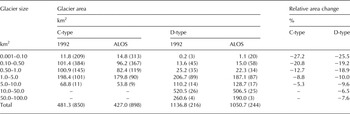
In total, 1290 glaciers covering 1515.6 ± 239.7 km2 were delineated from the 22 ALOS images from 2006 to 2010. Of these, 1034 were C-type glaciers (440.2 ± 33.3 km2) and 256 were D-type glaciers (1074.4 ± 206.4 km2) (Table 2). The mean areas of the C- and D-type glaciers were 0.43 and 4.16 km2, respectively, which is identical to the recent findings in the Bhutan Himalaya (Nagai and others, Reference Nagai, Fujita, Nuimura and Sakai2013). More than 80% of the glaciers in the study region are located between 5000 and 6500 m a.s.l., similar to the 75% reported for the Khumbu region by Thakuri and others (Reference Thakuri2014).
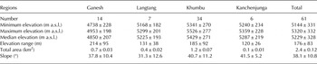
Table 2. Glacier parameters based on the ALOS glacier inventory for the eastern Nepal Himalaya

The massif divisions are shown in Figure 1a. The values in parentheses indicate the number of glaciers for each class, and the value after (±) denotes the standard deviation of the respective parameters.
Figure 5a, in which D-type and C-type glaciers are differentiated, shows the hypsometry of the 1992 and ALOS glacier inventories with 100 m resolution in elevation. D-type glaciers were found between 3400 and 8200 m a.s.l., with the maximum area (80.8 km2) at 5400–5500 m a.s.l., whereas C-type glaciers ranged from 4100 to 7700 m a.s.l., with the maximum area (46.9 km2) found at 5500–5600 m a.s.l. Both glacier types had their maximum areas in similar elevation bands (5400–5600 m a.s.l.), even though the distribution of D-type glaciers was considerably wider than the distribution of C-type glaciers, as was reported for the Bhutan Himalaya (Nagai and others, Reference Nagai, Fujita, Sakai, Nuimura and Tadono2016). Figure 5b shows glacier size plotted against the minimum and maximum elevations of each glacier from the ALOS inventory, in which a large spread of values was found for small size glaciers (<1 km2). In the case of larger glaciers (>1 km2), there is a clear dependency on both the minimum and maximum elevations, implying that larger glaciers tend to spread over a wide elevation range.

Fig. 5. (a) Hypsometry of the glaciers from the ALOS (thick lines) and the 1992 (thin lines) inventories, (b) relationship between glacier size with respect to maximum (green) and minimum (black) elevation in the ALOS inventory and (c) hypsometry of normalised area change along normalised elevation. In 5a and 5c, the debris-free (C-type, blue lines), debris-covered (D-type, red lines) and disappeared (black line) glaciers are distinguished.
The overall mean slope from the ALOS inventory was 32.6 ± 9.8°, with D-type glaciers being less steep (30.7 ± 8.7°) than C-type glaciers (37.2 ± 9.7°) (Table 2). The glaciers in this area exhibited orientations between SE and SW as our studied domain was confined to Nepalese territory and therefore to the southern side of the main Himalayan divide. We found that C-type glaciers are distributed uniformly throughout all orientations, whereas many D-type glaciers are concentrated in the NW–NE direction.
Figure 6a shows the normalised distribution (%) of glacier area and glacier number in all (total) and in the individual four massifs from the ALOS inventory. The studied domain was dominated by small (<1 km2) glaciers (1050) covering a small area (245 km2; 16% of the total), whereas medium and large glaciers (>1 km2) were fewer (240) but covered a larger area (1271 km2; 84% of the total) (Fig. 6a; Table 2). The normalised distributions (%) of the number and area of C- and D-type glaciers suggest that most C-type glaciers (931; 90%) were small glaciers (<1 km2) that covered 46% of the total area (204.1 km2 out of 440.2 km2), while the remaining 10% (103 in number) covered 54% of the area (236.1 km2 out of 440.2 km2). Similarly, for D-type glaciers, 119 (46%) were small (<1 km2) glaciers covering 40.4 km2 (4%), while the remaining 139 (54%) covered 1033.9 km2 (96%) (Fig. 6b).

Fig. 6. Normalised distribution (%) of area (solid lines) and number (dotted–dashed lines) of glaciers in terms of (a) all (total) and the four massifs and (b) C-type and D-type glaciers in the ALOS glacier inventory.
4.2. Regional statistics
As shown by Figure 1a and Table 2, the Khumbu massif has the most extensive ice cover, followed by the Kanchenjunga massif. The Langtang and Ganesh massifs have the smallest coverage. The eastern massifs, Kanchenjunga and Khumbu, are dominated by D-type glaciers, whereas C-type glaciers are prevalent in the western massifs. Figure 7a shows the hypsometry of the glaciers from the ALOS inventory for all four massifs. Most of the glaciers in the region are located between 5000 and 6500 m a.s.l., but the massifs show different hypsometric modes. The eastern massifs, Khumbu and Kanchenjunga, dominated mostly by D-type glaciers, showed a larger elevation range than the western massifs, Ganesh and Langtang. From the normalised elevation and area distributions (Fig. 7b), we found that glaciers in the Ganesh and Langtang massifs had their greatest area in the middle of their elevation range, whereas glaciers in the Khumbu and Kanchenjunga massifs were skewed slightly to lower elevation because of the larger dominancy of debris-covered parts in these massifs. A similar trend was reported in the South Asia East region by Pfeffer and others (Reference Pfeffer2014). Figure 8a shows the spatial distribution of mean glacier elevation for the entire study area. The figure suggests that elevation increases noticeably from south to north because precipitation decreases toward the north due to the orographic barrier (Bookhagen and others, Reference Bookhagen and Burbank2006; Salerno and others, Reference Salerno2015).

Fig. 7. Hypsometry of (a) the surviving glaciers and normalised hypsometry of (b) the surviving glaciers and (c) the disappeared glaciers in the four massifs from the ALOS glacier inventory. Dotted line in (b) is of mountain glacier suggested by Raper and Braithwaite (Reference Raper and Braithwaite2006).

Fig. 8. Spatial distribution of (a) mean elevation for all of the glaciers in the ALOS glacier inventory and (b) relative area change (%) for C-type glaciers. A sample of 478 glaciers from 0.1 to 1 km2 was chosen to de-bias the distribution.
The eastern three massifs of Kanchenjunga, Khumbu and Langtang had relatively gentler slopes, whereas glaciers in the westernmost Ganesh massif were remarkably steep due to its large dominance of small glaciers (Table 2). For all massifs, D-type glaciers were less steep than C-type glaciers because of their larger size (Fig. 6b). Although most of the glaciers were south facing, some showed a slightly different orientation, such as in the westernmost Ganesh massif (N–NE) and in the easternmost Kanchenjunga massif (W–NW). The normalised distributions of glacier number and area showed a similar pattern for the different size classes, in which a large number of small glaciers cover a small area and fewer medium and large glaciers cover most of the area (Fig. 6a).
4.3. Glacier changes over the entire domain
For glaciers that exactly matched between the two inventories, the total area decreased from 1616.7 ± 247.7 km2 in the 1992 inventory to 1477.8 ± 232.5 km2 in the ALOS inventory, giving a −8.5% area change (−0.5 ± 0.1% a−1) during the study period. This rate, however, does not change when considering the disappeared glaciers because of their very small surface area (2.4 ± 0.12 km2). A slight increase in the number of glaciers from 1066 to 1142 (7%; Fig. 3) resulted from fragmentation, as also reported for the Nepal and Bhutan Himalayas (Bajracharya and others, Reference Bajracharya, Maharjan, Shrestha, Bajracharya and Baidya2014a, Reference Bajracharya, Maharjan and Shresthab). An example of glacier changes over the study period along with their fragmentation is shown in Figure 4c for the Kanchenjunga massif. In total, 850 C-type and 216 D-type glaciers from the 1992 glacier inventory were compared with 898 C-type and 244 D-type glaciers from the ALOS glacier inventory (Fig. 3). The area of C-type glaciers changed from 481.3 ± 35.9 km2 in the 1992 glacier inventory to 427.0 ± 32.0 km2 in the ALOS glacier inventory, giving an area change of −11.20% (−0.70% a−1), whereas the area of D-type glaciers changed from 1136.8 ± 212.9 km2 to 1050.7 ± 200.5 km2, giving an area change of −7.50% (−0.47% a−1) during the study period.
Figure 9a shows the relationship between the relative area change (%) and glacier area for both C- and D-type glaciers, also presented in Table 3 for different size classes. Small C-type glaciers, predominant in number, lost a larger proportion of their area, i.e. >40% in many cases, whereas medium and large C-type glaciers lost a smaller proportion (~20%) of their area. Likewise, small D-type glaciers (<10 km2) lost a larger proportion of their area than did large D-type glaciers (>10 km2), which were confined to <20% loss. Hence, small glaciers lost a larger proportion of their area than large glaciers, which confirms that glacier change was largely dependent on original size. The relative area change (%) for C-type glaciers was found to be slightly higher than that for D-type glaciers, with median values of −13.7% (p < 0.0001) and −9.5% (p < 0.01), respectively (Fig. 9b), which was also reported in the wide range of the Himalayas (Scherler and others, Reference Scherler, Bookhagen and Strecker2011).

Fig. 9. (a) Relationship between glacier area in the 1992 glacier inventory and relative area change (%), in which C-type (blue circles), D-type (red circles) and disappeared (black dots) glaciers are discriminated, and (b) box plot of relative area change (%) for C-type and D-type glaciers. Width, upper and lower bounds of the box, thick black line, and solid black circle denote number of glaciers, the first and third quartile, median and average of the change, respectively. Whiskers extend 1.5 times of the interquartile range.
Table 3. Glacier area (km2) and their respective number (in parenthesis) for 1992 and ALOS inventory (both C-type and D-type)
Average of relative area change (%) for both C-type and D-type glaciers in different size classes.
We also investigated the change in glacier area as a function of elevation by comparing the hypsometry of the 1992 and ALOS inventories for both C-type and D-type glaciers (Fig. 5a). Based on the third quartiles of the area change, C-type glaciers and D-type glaciers shrank noticeably below 5750 m a.s.l and 5950 m a.s.l., respectively. Even though the patterns of shrinkage were similar for both types, the normalised distribution (%) of area change with elevation suggests that most of the C-type glaciers lost the major part of their area in a lower elevation zone than that of the D-type glaciers (Fig. 5c).
4.4. Disappeared glaciers
No previous study has reported the complete disappearance of glaciers in the eastern Nepal Himalaya. To cross check the existence of glaciers and their topographical orientation, we overlaid four Landsat TM images from the 1992 post-monsoon season (Table 1) on the 1992 glacier inventory. In total, 61 (5%) C-type small glaciers covering 2.4 ± 0.3 km2 (0.1%), and ranging in size from 0.01 to 0.20 km2 (average of 0.04 km2) completely disappeared during the study period (Figs 1b, 9a; Table 4), which is comparatively less than in northern Patagonia, where 374 small glaciers (<0.50 km2) out of 1664 (22%) completely disappeared during 1985–2011 (Paul and Mölg, Reference Paul and Mölg2014). Within the study region, the Ganesh and Khumbu massifs had the largest area losses in terms of number of disappeared glaciers (14 and 34, respectively) since 1992, corresponding to area losses of −0.7 ± 0.1 km2 and −1.2 ± 0.1 km2, respectively, compared with those of the Langtang (0.4 ± 0.02 km2) and Kanchenjunga (0.1 ± 0.01 km2) massifs. Figure 7c shows the normalised distribution (%) of disappeared glaciers for all massifs, and it reveals that most of the disappeared glaciers were located in lower elevation zones.
Table 4. Characteristics of the disappeared glaciers in the four massifs of the eastern Nepal Himalaya
The value after (±) denotes the standard deviation of the respective parameters.
5. DISCUSSION
5.1. Rates of glacier area change in the eastern Nepal Himalaya
Previous studies have reported a wide range of change rates in glacier area along the Himalayas and in neighboring regions over the last couple of decades (Fig. 10). For instance, Ye and others (Reference Ye, Kang, Chen and Wang2006) and Yao and others (Reference Yao2012) showed relatively lower change rates in glacier area for the Tibetan Plateau (TP) compared with the Nepal Himalaya (NH) and the Bhutan Himalaya (BH). Kulkarni and others (Reference Kulkarni2007, Reference Kulkarni, Rathore, Singh and Bahuguna2011) found that glaciers in the western Indian Himalaya (IH) changed at rates of −0.54 and −0.41% a−1, which is significantly more negative than for the eastern Sikkim Himalaya (SK, −0.16% a−1; Basnett and others, Reference Basnett, Kulkarni and Bolch2013) and the Kanchenjunga–Sikkim area (KJ, −0.23% a−1; Racoviteanu and others, Reference Racoviteanu, Arnaud, Williams and Manley2015). A significant discrepancy was found in the BH, where Karma and others (Reference Karma, Ageta, Naito, Iwata and Yabuki2003) reported a less negative rate of area change (−0.27% a−1) than the −0.78% a−1 reported recently by Bajracharya and others (Reference Bajracharya, Maharjan and Shrestha2014b). Such a significant discrepancy may be due to differences in data quality (e.g. snow conditions), sample size, map interpretation and study period, as toposheets (1 : 50 000) from the 1960s and SPOT images (20 m resolution) from December 1993 were used by Karma and others (Reference Karma, Ageta, Naito, Iwata and Yabuki2003) whereas only Landsat images (1980–2010) were used by Bajracharya and others (Reference Bajracharya, Maharjan and Shrestha2014b). The large uncertainty associated with the 1960s toposheets may be the main reason for the difference, even though recent acceleration of glacier shrinkage may have also contributed. Nie and others (Reference Nie, Zhang, Liu and Zhang2010) investigated glacier extent on the southern (ES) and northern (EN) slopes of the Mount Everest region based on the normalised difference snow/ice index (NDSII) and found a slightly faster shrinkage for the southern flank (−0.56% a−1) than for the northern flank (−0.48% a−1). Bolch and others (Reference Bolch, Buchroithner, Pieczonka and Kunert2008) investigated glaciers in the Khumbu region based on multitemporal imagery from 1962 (Corona KH-4), 1992 (Landsat TM) and 2005 (Terra ASTER) and reported a much less negative area change (−0.12% a−1) than the values given above. Recent studies for the Khumbu region reported contradictory areal change rates, such as −0.27% a−1 (1962–2011; Thakuri and others, Reference Thakuri2014) and −0.59 ± 0.17% a−1 (1976–2009; Shangguan and others, Reference Shangguan2014), even though the analysed periods were similar. Although glacier outlines were digitised manually in both of these studies, one reason for the different shrinkage rate stated by Shangguan and others (Reference Shangguan2014) may be the data quality because 39 toposheets (1 : 50 000 and 1 : 100 000), based on aerial photography between 1971 and 1980 (by the Chinese military geodetic service) were chosen for the glacier delineation. In addition to data quality, snow condition of images, different size class distributions, interpretation of debris cover area and consideration of steep glaciers at higher elevations might be major sources of such variability.

Fig. 10. Rates of area change from different studies for glaciers around the Himalayas: Everest South (ES), Tibetan Plateau (TP), Sikkim (SK), Kanchenjunga (KJ), Bhutan Himalaya (BH), Indian Himalaya (IH), Nepal Himalaya (NH), Everest North (EN) and Koshi Basin (KB).
Unlike other studies considering only the full sample of, our study reports changes of −0.50, −0.47, and −0.70% a−1 for all, D-type and C-type glaciers, respectively. Comparing with other studies, we obtained an areal rate change (−0.50% a−1) similar to the −0.56% a−1 from Nie and others (Reference Nie, Zhang, Liu and Zhang2010) for all glaciers, but a considerably larger area loss (−0.70% a−1) was reported for C-type glaciers compared with the −0.24% a−1 from Bolch and others (Reference Bolch, Buchroithner, Pieczonka and Kunert2008). C-type glaciers are expected to exhibit a larger area loss than D-type glaciers because debris cover might substantially reduce ablation (Scherler and others, Reference Scherler, Bookhagen and Strecker2011). Another reason for the high rate of shrinkage may be our investigation period, which was shorter and more recent than that of previous studies, including the period of glacier shrinkage acceleration (Zemp and others, Reference Zemp2015).
5.2. Regional analysis of the area change distribution
Figure 8b shows the spatial distribution of the relative area change (%) for C-type glaciers in the eastern Nepal Himalaya, which ranges from 0.0 to −62.0% during the study period. As change rates are size dependent and only changes of the same size class should be compared (Fig. 9a), we sampled 478 glaciers from the same size range (0.1–1.0 km2). The entire domain was dominated mostly by small and medium relative area changes (0 to −25%), with some larger changes (−50 to −62%).
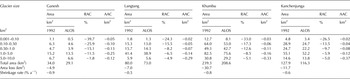
The relative area change (%) and the absolute area change (km2) in the four massifs show higher values of relative area change for small glaciers and higher values of glacier area change for large glaciers (Table 5). The Ganesh massif glaciers clearly suffered greater area loss (median of −0.08 km2) than the Langtang (median of −0.04 km2), Khumbu (median of −0.04 km2) and Kanchenjunga (median of −0.03 km2) massifs (Fig. 11). Although there were fewer glaciers (44) in the Ganesh massif, the difference in area change was statistically significant (p < 0.0001; Student's t test). The reason for the stronger changes of the glaciers in the Ganesh massif may be their steepness (Table 2), because steeper glaciers are smaller and therefore more predisposed to higher relative area change (Fig. 9a). Another plausible reason is their shorter response time because they change faster to climate change. Similar results, in which steeper glaciers lost larger area, were reported in the Kanchenjunga–Sikkim (Racoviteanu and others, Reference Racoviteanu, Arnaud, Williams and Manley2015) and Khumbu regions (Salerno and others, Reference Salerno, Buraschi, Bruccoleri, Tartari and Smiraglia2008).
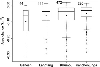
Fig. 11. Glacier area change for the four massifs studied in the eastern Nepal Himalaya. The box width denotes the glacier number. The upper and lower bounds of the box, thick lines and solid circles denote the first and third quartiles, median and average of the area change, respectively. The whiskers extend 1.5 times the interquartile range from the box. Outliers beyond −0.40 km2 (one in Ganesh, four in Khumbu and one in Kanchenjunga) are not shown.
Table 5. Shrinkage rate for individual massif where area from 1992 and ALOS inventory is depicted and average of relative area change (RAC) and absolute area change (AAC) of C-type glaciers for all the four massifs in the different size classes
5.3. Area loss and topographical settings
Correlations between glacier area changes and topographic variables such as minimum elevation and slope were examined using the Pearson's correlation coefficient. Aspect was not examined because the study domain was limited to Nepalese territory and thus south biased. A moderate but significant correlation was found between area change and minimum elevation (r = 0.30, p < 0.0001), indicating that glaciers that reached further down lost more area. The most significant negative correlations were found for elevation range (r = −0.50, p < 0.0001) and glacier size (r = −0.62, p < 0.001), suggesting that larger glaciers lost more area. A weak but significant correlation was also found for mean slope (r = 0.16, p < 0.0001), which may result from larger glaciers tending to have gentler slopes covered mostly by debris.
6. CONCLUSIONS
We delineated 1290 glacier polygons across the eastern Nepal Himalaya using high-resolution ALOS images (2.5 m) from 2006 to 2010 and compared them with another set of glacier polygons created with aerial photographs from 1992. Unlike previous studies, which were limited to the Mount Everest region, this study had an expanded coverage from the Ganesh massif in the west to the Kanchenjunga massif in the east. This study also analysed C- and D-type glaciers separately. The entire area showed moderately high rates of glacier change since 1992: −0.50% a−1 for all glaciers, −0.47% a−1 for D-type glaciers and −0.70% a−1 for C-type glaciers, values similar to the uncorrected average value (−0.57% a−1) reported by Cogley (Reference Cogley2016) for all of high mountain Asia. We also found higher shrinkage rates for the eastern Nepal Himalaya than those reported for surrounding areas. Smaller glaciers, especially of C-type, are shrinking faster than larger glaciers. The intra-regional analysis showed statistically significant higher shrinkage rates for the western Ganesh massif than for the eastern massifs. A significant number of small glaciers, covering an area of 2.4 km2, have completely disappeared since 1992. Although climatic interpretation is not within the scope of this study, the recent temperature and precipitation changes could be a plausible explanation for the glacier shrinkage, which requires further investigation as more ground observations become available.
ACKNOWLEDGEMENTS
We thank the scientific editor, M. Tranter, and the reviewers, G. Cogley and F. Paul, for their constructive and invaluable suggestions. This study was supported by a grant from the Funding Program for Next Generation World-Leading Researchers (NEXT Program, GR052) and Grants-in-Aid for Scientific Research (26257202) from the Japan Society for the Promotion of Science.
AUTHOR CONTRIBUTION STATEMENT
K. F. and A. S. designed the study. S. O. delineated the glacier outlines of the ALOS glacier inventory and analysed the data. K. A. created and provided the 1992 glacier inventory. A. S., D. L., T. N. and H. N. established the methodology to delineate the glacier outlines. S. O. and K. F. wrote the paper. All authors contributed to the discussion of the study.


 Open access