The Link between the Physical and Chemical Properties of Carbon-Bearing Melts and Their Application for Geophysical Imaging of Earth’s Mantle

7 - The Link between the Physical and Chemical Properties of Carbon-Bearing Melts and Their Application for Geophysical Imaging of Earth’s Mantle

Published online by Cambridge University Press: 03 October 2019

Tahar Hammouda and

Edited by

Isabelle Daniel and

Beth N. Orcutt: Affiliation:
Bigelow Laboratory for Ocean Sciences, Maine
Isabelle Daniel: Affiliation:
Université Claude-Bernard Lyon I
Rajdeep Dasgupta: Affiliation:
Rice University, Houston

Book contents

Summary

Significant investment in new capacities for experimental research at high temperatures and pressures have provided new levels of understanding about the physical properties of carbon in fluids and melts, including its viscosity, electrical conductivity, and density. This chapter reviews the physical properties of carbon-bearing melts and fluids at high temperatures and pressures and highlights remaining unknowns left to be explored. The chapter also reviews how the remote sensing of the inaccessible parts of the Earth via various geophysical techniques – seismic shear wave velocity, attenuation, and electromagnetic signals of mantle depths – can be reconciled with the potential presence of carbon-bearing melts or fluids. Supplemental online material is available for this chapter at www.cambridge.org/9781108477499#resources.

Keywords

mantle somatism incipient melt adiabatic mantle melt carbonate melt silicate melt melt density melt mobility mantle convection

Information

Type: Chapter
Information: Deep Carbon
Past to Present
, pp. 163 - 187

DOI: https://doi.org/10.1017/9781108677950 [Opens in a new window]

Publisher: Cambridge University Press

Print publication year: 2019
Creative Commons: This content is Open Access and distributed under the terms of the Creative Commons Attribution licence CC-BY-NC-SA 4.0 https://creativecommons.org/cclicenses/

7 The Link between the Physical and Chemical Properties of Carbon-Bearing Melts and Their Application for Geophysical Imaging of Earth’s Mantle

7.1 Introduction: Toward a Geophysical Definition of Incipient Melting and Mantle Metasomatism

Geochemical observations on mantle xenoliths and experiments at pressure and temperature on CO₂- and H₂O-bearing mantle rocks have provided the widely accepted picture that melts and fluids are flowing and reacting within the solid mantle.Reference Wallace and Green¹^–Reference Dasgupta⁷ Whether this must be seen as a transient and local process or a broad and planetary-scale mantle dynamic is unknown.Reference Aulbach, Massuyeau and Gaillard²^, Reference O‘Reilly and Griffin⁴^, Reference Dasgupta⁷ Understanding this could establish whether these melt advection processes explain some remote geophysical observations and could help with clarifying the geodynamic roles played by these melting dynamics. The question is rendered difficult since these melts may not be easily linked to the volcanic products reaching Earth’s surface; somehow, most of the mantle melting processes may produce melts that never leave the mantle and therefore remain inaccessible.

The fingerprints of such deep melts have been historically characterized by geochemical means: trace element abundances and some isotopic ratios of mantle xenoliths are modified by the reactive passage of these melts.Reference Aulbach, Massuyeau and Gaillard²^, Reference O‘Reilly and Griffin⁴^, Reference Tappe⁶^, Reference Coltorti⁸^, Reference Pilet, Baker and Stolper⁹ Major element abundances and the modal proportions of minerals can also be significantly affected.Reference Tappe⁶^, Reference Coltorti⁸ All of this is named mantle metasomatism,Reference Aulbach, Massuyeau and Gaillard²^, Reference Coltorti⁸^, Reference Pilet, Baker and Stolper⁹ and this process may explain some geophysical observations.Reference Aulbach, Massuyeau and Gaillard²^, Reference Pinto¹⁰ Notably, mantle metasomatism has been characterized on lithospheric samples only, therefore representing the shallowest part of a deeper melting dynamic that will be presented hereafter.

The melt causing such modifications is usually not observable in mantle rocks and is also not generally found in most volcanic exposures (except for the enigmatic petit-spot volcanoesReference Hirano¹¹). Experimental petrology has therefore been used to reconstruct the chemical compositions of the parental melt coexisting at equilibrium with the solid mantle assemblage.Reference Dasgupta³^, Reference Hammouda and Keshav⁵^, Reference Dasgupta⁷^, Reference Wyllie and Huang¹²^, Reference Taylor and Green¹³ Experiments at upper-mantle conditions have shown the key role of volatile species (i.e. H₂O and CO₂) in stabilizing CO₂-rich melts or fluid versus SiO₂-rich melts.Reference Wallace and Green¹^, Reference Dasgupta³^, Reference Hammouda and Keshav⁵^, Reference Dasgupta⁷^, Reference Wyllie and Huang¹²^, Reference Taylor and Green¹³ The take-home message of such experimental approaches is that, in the presence of volatiles, mantle melting can occur in most of the upper mantle;Reference Dasgupta⁷ melting regions are commonly limited by redox process reactions favoring diamonds in the deep upper mantle and decarbonation reactions in the shallowest part of the mantle.Reference Hammouda and Keshav⁵^, Reference Dasgupta⁷^, Reference Stagno, Ojwang, McCammon and Frost¹⁴

The particularity of the mantle melting regime due the presence of H₂O and CO₂ is that it produces small amounts of melt (i.e. <1%) embedded within the solid mantle matrix. These small amounts of melt, named incipient melt, are directly linked to small amounts of H₂O and CO₂ (i.e. tens to thousands of part per millions (ppm)) being present in the mantle.Reference Le Voyer, Kelley, Cottrell and Hauri¹⁵ These incipient melts are very CO₂ and H₂O rich. Their volatile-rich nature imparts physical properties to these melts that are at odds with the conventional basaltic products that reach Earth’s surface. A large part of this chapter will review the state of the art on the unconventional properties of these CO₂–H₂O-rich melts.

What are the origins of these melts? They are certainly diverse and linked to large-scale recycling processes, but broadly speaking, mantle convection (large or small scaleReference Morency, Doin and Dumoulin¹⁶^–Reference French, Lekic and Romanowicz¹⁸) causes decompression melting in many mantle regions. In the upper mantle, convection occurs in the asthenosphere – the convective mantle. Upwelling regions undergo decompression and produce incipient melts. The asthenosphere remains enigmatic as we do not have any mantle xenolith samples from it. Mantle xenoliths are lithospheric, being part of the plates. The mantle metasomatic processes captured from mantle xenoliths therefore describe what happens to these melts when they reach the top of the convection limbs and meet the base of tectonic plates.

The repetitive passage of small amounts of melts and their freezing and reactivity with solids can result in major geodynamic modifications. Seminal examples of reactive transports of melts within an ancient lithosphere achieving a sort of completion are reported as cases of rejuvenation.Reference Aulbach, Massuyeau and Gaillard²^, Reference Tappe⁶ By this process, lithospheres, being thick, cold, depleted, and rigid lids, can become the warm, enriched, and soft asthenosphere. This means that the boundary between the nonconvective and the convective mantle, the so-called lithosphere–asthenosphere boundary (LAB), must be partly controlled by melt advection–reaction processes.Reference Aulbach, Massuyeau and Gaillard²^, Reference O‘Reilly and Griffin⁴ The LAB must be, at a geological timescale, a movable boundary.Reference O‘Reilly and Griffin⁴^, Reference Tappe⁶ Notably, though this is not further discussed here, in addition to mass transfer processes, melt advection at the LAB also conveys heat (including latent heatReference Keller and Katz¹⁹).

A critical issue is whether such small melt fractions can be detected using remote geophysical probing of the electrical conductivity (EC) and seismic properties of Earth’s mantle.Reference Eggler²⁰^, Reference Gaillard²¹ This requires the long-studied geochemical processes of mantle melting and metasomatism to be converted into the physical numbers that are addressed by geophysical probing. This also requires issues regarding the fluid mechanics of melt advection in the mantle to be tackled (i.e. how fast the incipient melt moves with respect to conventional convection rates and plate velocities).

Here, we address the stability domains, the atomic structures, and the physical properties of these incipient melts together with their connectivity at small-volume fractions in mantle aggregates. The objective of this assessment is to highlight the possible links between mantle melting–metasomatism and the geophysical observations that supposedly mark the LAB.

These geophysical observations indicate bright contrasts between resistive mantle lids also featuring high seismic wave velocities (V_P and V_S) and the underlying conductive mantleReference Naif, Key, Constable and Evans²²^, Reference Kawakatsu and Utada²³ also featuring low V_S.Reference Kawakatsu and Utada²³^–Reference Schmerr²⁵ The seismic discontinuities have been named as the Gutenberg discontinuity (G)Reference Schmerr²⁵ and the underlying region is the low-velocity zone (LVZ). This broad description is not a rule, as there are specific settings where such bright contrasts are not clearly observed, such as beneath cratonsReference Eaton²⁶ and in the enigmatic NoMelt area,Reference Sarafian²⁷ a setting in the Pacific Ocean where no geodynamic perturbations seem to operate. We also note that the depth of this geophysical discontinuity varies from being shallow beneath oceanic plates (50–90 km) to being deep (and elusive) under cratons (>200 km). The cause of low V_S and high conductivity remain debated; it does not have to be a unique cause, but a common explanation would be an elegant simplification. Whether these discontinuities reveal the ponding of melts is an increasingly accepted though still debated concept.Reference Kawakatsu and Utada²³^, Reference Schmerr²⁵ Here, we will focus on the melting processes that are able to cause anomalously high ECs because the effect of melting on the genesis of the LVZ remains elusive.Reference Schmerr²⁵

7.2 CO₂-Rich Melts in the Mantle: Stability, Composition, and Structure

7.2.1 Partial Melting in the Presence of CO₂ and H₂O: Incipient Melting

The fluxing effect of volatiles on silicate melting has been long recognized.Reference Wallace and Green¹^, Reference Dasgupta³^, Reference Hammouda and Keshav⁵^, Reference Dasgupta⁷^, Reference Wyllie and Huang¹²^–Reference Stagno, Ojwang, McCammon and Frost¹⁴ In the case of mantle melting, the effects of H₂O and CO₂, whether separatelyReference Dasgupta³^, Reference Wyllie and Huang¹²^, Reference Stagno, Ojwang, McCammon and Frost¹⁴^, Reference Hirschmann, Tenner, Aubaud and Withers²⁸ or mixed,Reference Wallace and Green¹^, Reference Dasgupta³^, Reference Dasgupta⁷^, Reference Taylor and Green¹³^, Reference Massuyeau, Gardés, Morizet and Gaillard²⁹^, Reference Hirschmann³⁰ have been investigated. It is clear that peridotite systems equilibrated with H₂O–CO₂ mixtures have been poorly investigated in comparison to the (nominally) CO₂-only bearing system.Reference Hammouda and Keshav⁵

Figure 7.1 summarizes the main features for the case of melting at undersaturated CO₂–H₂O fluid conditions. In the temperature region below the fluid-free high-pressure solidus, the amount of melt is controlled by the low amount of available fluid. This melting regime is incipient melting. In the incipient melting regime, several cases must be highlighted.

Figure 7.1

Pressure–temperature plot showing the stability fields for different types of mantle melt as a function of the volatile contents. Different geotherms (10 My, 80 My, cratons) are superimposed. The CO₂-bearing hydrous peridotite solidus is calculated from the combination of solidus temperatures of Ref. 1 from 0 to ~4 GPa and Ref. 13 at higher pressures. We connected the melting curve of CO₂-bearing hydrous peridotite to that of the dehydration solidus of nominally anhydrous peridotiteReference Hirschmann, Tenner, Aubaud and Withers²⁸ (considering peridotite with 460 ppm H₂O) at low pressures.

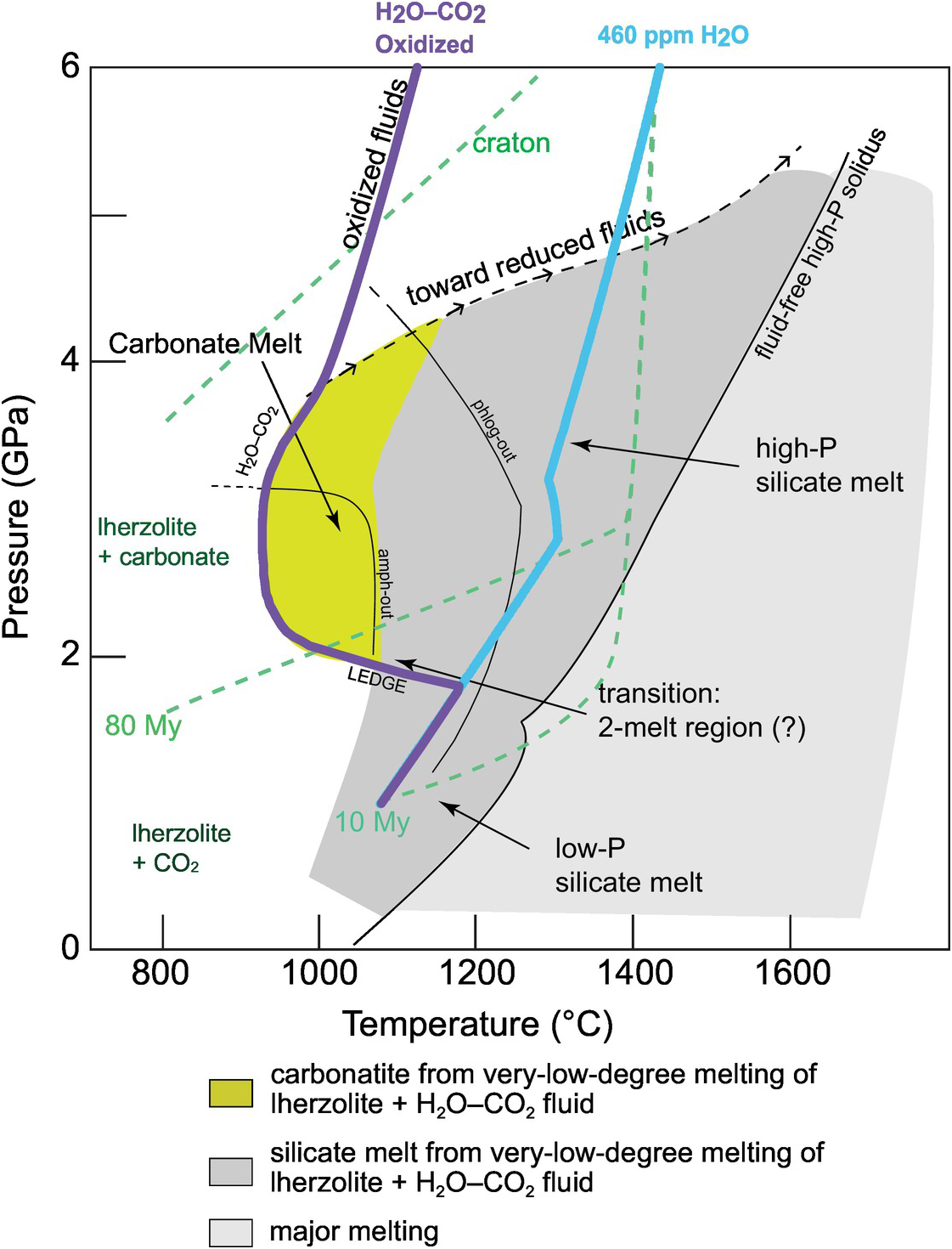
For pressures less than 2 GPa (corresponding to depths of less than 60 km), the solidus is weakly depressed. In this pressure range, the solubility of CO₂ in silicate melts is low, most CO₂ is in the fluid, and the solidus is controlled by the availability of water.Reference Hirschmann, Tenner, Aubaud and Withers²⁸

At ~2 GPa, the CO₂ of the fluid reacts with the silicates, yielding carbonate mineral formation. This carbonation reaction has the effect of strongly depressing the solidus temperature, and the carbonate ledge (i.e. nearly isobaric melting curve) is developed in the phase diagram. Melts at the solidus are carbonatitic.Reference Wallace and Green¹^, Reference Dasgupta³^, Reference Dasgupta⁷^, Reference Massuyeau, Gardés, Morizet and Gaillard²⁹ Away from the solidus, hydrated silicate melting takes places and the melt compositions shift from carbonatitic to carbo-hydrous silicates.Reference Dasgupta³^, Reference Dasgupta⁷^, Reference Massuyeau, Gardés, Morizet and Gaillard²⁹ As long as the temperature remains below that of the fluid-free solidus, the amount of produced melt is controlled by the fluid availability. Major melting only happens as the fluid-free solidus is crossed (temperature >1350°C at 2 GPa).

As pressure is further increased, the CO₂–H₂O fluid may be reduced by interaction with mantle silicates.Reference Dasgupta³^, Reference Hammouda and Keshav⁵^, Reference Taylor and Green¹³^, Reference Stagno, Ojwang, McCammon and Frost¹⁴ Along the mantle geotherm, carbonate reduction following this reaction would occur at about 120–250 km depth.Reference Hammouda and Keshav⁵^, Reference Stagno, Ojwang, McCammon and Frost¹⁴ In the presence of hydrogen, a mixed CH₄–H₂O fluid is formed.Reference Taylor and Green¹³ In this fluid, water activity is lowered, resulting in increasing solidus as depth (and therefore reduction) increases. The solidus evolution caused by fluid reduction at high pressure is indicated by the dashed line with arrows in Figure 7.1.

7.2.2 Carbonate to Silicate Melts in Various Geodynamic Settings

Following this broad picture of the process of incipient melting, we present here the range of melt compositions produced in various geodynamic settings. Two end-member cases are illustrated: adiabatic conditions showing regions where volcanism occurs at Earth’s surface versus intraplate conditions showing mantle melting without volcanism.

Figure 7.2 illustrates melting along an adiabatic mantle (i.e. convective mantle) involving various H₂O- and CO₂-enrichmentsReference Le Voyer, Kelley, Cottrell and Hauri¹⁵ and a potential temperature of 1360°C. The calculated meltsReference Massuyeau, Gardés, Morizet and Gaillard²⁹ define an array of compositions ranging from low to high silica content in response to decompression melting: incipient melts evolving from carbonatite (i.e. <15 wt.% SiO₂), to carbonated basalts (15–50 wt.% SiO₂), to alkali basalts (SiO₂ >40 wt.%). Hereafter in the chapter, some of these compositions are used as reference compositions for which density, viscosity, and EC are defined (stars in Figure 7.2; see Section 7.3). Decreasing the bulk volatile contents decreases the absolute depth and the depth interval at which the equilibrium melt composition changes from carbonate to silicate melts: while the volatile-enriched mantle can produce silicate-bearing liquids down to 250 km, the volatile-depleted case shows an abrupt shift in composition at ~100 km depth within a ~10–20‑km interval. This indicates that dry systems must have a greater tendency for carbonate–silicate immiscibility. Notably, Figure 7.2 does not consider the possibility of redox melting at ~250 km depth.

Figure 7.2

Melt composition (left) and melt fraction (right) produced during adiabatic mantle melting (temperature = 1360°C or 1480°C when specified). Under most of the pressure–temperature–volatile content conditions shown here, incipient melting occurs. Incipient melting of depleted (100 ppm H₂O–100 ppm CO₂) to enriched (500 ppm) mantle sources is considered. The stars show compositions for which viscosities were determined by molecular dynamics (see Section 7.3).

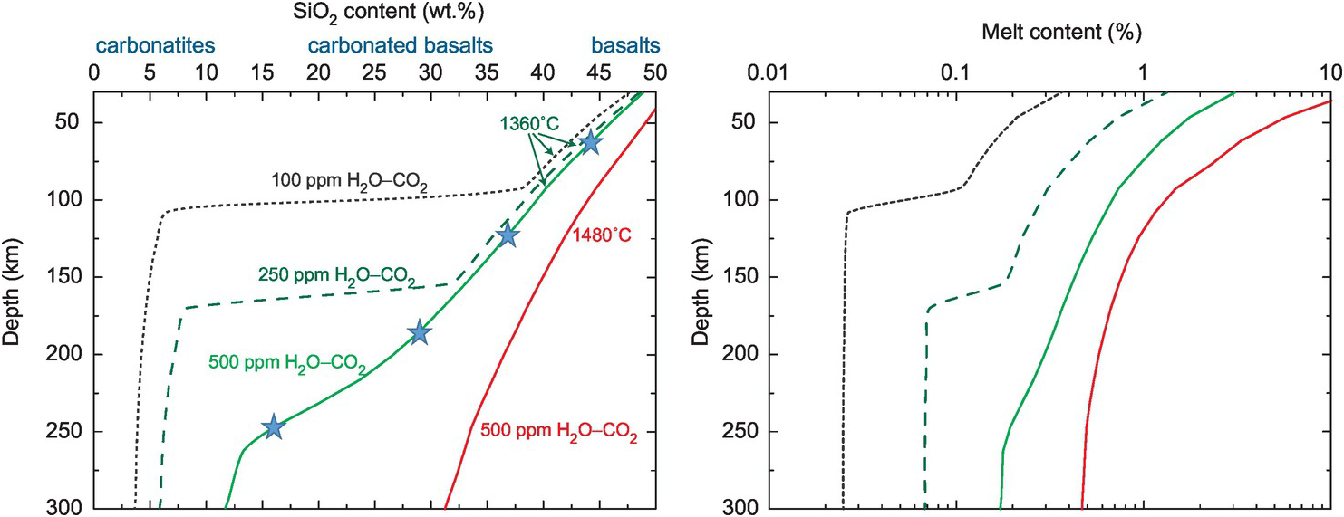
Figure 7.3 illustrates the nature of equilibrium partial melts formed in an intraplate thermal regime considering both CO₂–H₂O depleted and enriched mantles. A young plate (10 Ma, red), an intermediate plate (80 Ma, green), and a craton (gray) are illustrated.Reference McKenzie, Jackson and Priestley³¹ These lithospheres of variable ages, and therefore variable thicknesses, can host melts with contrasting and strongly depth-dependent compositions. These lithospheres overlay a convective mantle having an age-independent pressure–temperature–melt composition pattern. The lithospheric and convective mantles are, by definition, separated by a thermal boundary layer, the LAB, separating the diffusive (lid) and the adiabatic (convective) mantles.Reference McKenzie, Jackson and Priestley³¹ To what extent discontinuities in ECsReference Naif, Key, Constable and Evans²²^, Reference Kawakatsu and Utada²³ and seismic wave velocitiesReference Schmerr²⁵^, Reference Burgos³² map the depth of this thermal LAB is a matter of a great debate. The depth range of the putative seismic G as broadly compiled from various studies and for various geodynamic environments is shown in Figure 7.3.Reference Naif, Key, Constable and Evans²²^, Reference Kawakatsu and Utada²³ Notice that G values are reported at depths of ~60–80 km for oceanic lithospheres of variable ages (0–120 Ma),Reference Kawakatsu and Utada²³^, Reference Schmerr²⁵ while the conventional LAB depths for similar lithospheric ages vary over a range of 0–110 km.Reference McKenzie, Jackson and Priestley³¹ We must also notice that the seismic signal of G may be manifold and feature variable depth–age relationships.Reference Burgos³²

Figure 7.3

Profiles of melt compositions in intraplate geodynamic settings of variable ages (cratons, 80 Ma, and 10 Ma from left to right) compared to the depth range of the Gutenberg discontinuity (G) and the LVZ. The curve labeled “LAB” corresponds to the thermal lithosphere–asthenosphere boundary. The LAB displays a depth that changes with the age of the plate.Reference McKenzie, Jackson and Priestley³¹ One sees that the degree of H₂O–CO₂ enrichment moderately affects the type of melt composition formed at lithospheric depth. It is essentially the temperature change with depth that controls the melt composition. This narrow range of lithospheric melt compositions is at odds with the large range of melt compositions that are formed in the convective mantle, which strongly depends on the degree of H₂O–CO₂ enrichment, as shown in Figure 7.2.

The broad correspondence between the stability field of incipient melting and the geophysical signals supposed to mark the LAB has long been known.Reference Dasgupta³^, Reference O‘Reilly and Griffin⁴^, Reference Dasgupta⁷^, Reference Eggler²⁰^, Reference Hirschmann³⁰^, Reference Sifré³³ These observations must be advanced by considering the physical properties of incipient melts and how they impact the mantle rock properties near to the LAB.

7.2.3 Structural Differences between Silicate and Carbonate Melts

From a structural viewpoint, silicate and carbonate melts are opposites. However, they are end members of a continuum going from network-forming iono-covalent silicate liquids (e.g. silica) to ionic carbonate liquids (e.g. molten salts). The former are characterized by their degree of polymerizationReference Mysen and Richet³⁴ (estimated from the NBO/T ratio, with “NBO” being the number of nonbridging oxygens and “T” the number of tetracoordinated cations, Si and Al), whereas the latter are fully depolymerized, with the liquid structure being controlled by the size ratio between anions and cations and by the ion valence state.Reference Jones, Genge and Carmody³⁵ The microscopic structure of silicate melts is also quantified using structural indicators such as the Q_n species (with n = 0–4, where “n” is the number of TO₄ tetrahedra sharing a common oxygen) and the coordination numbers associated with the network-forming and network-modifying cations (e.g. Nc ≈ 4 for Si and Al, and Nc ≈ 5 – 8 for Fe, Mg, Ca, and Na).

In carbonate melts, experimental and simulation studiesReference Jones, Genge and Carmody³⁵^–Reference Vuilleumier, Seitsonen, Sator and Guillot³⁸ have shown that the number of carbonate ions (playing the role of O^2– in silicate melts) around Mg and Ca is about five to six, with one oxygen of each carbonate ion pointing preferentially toward the cation (with d_Mg–O = 2.0 Å and d_Ca–O = 2.35 Å, distances similar to those found in silicate melts), whereas the number of carbonate ions around each carbonate is about 12, a value similar to the oxygen coordination number in depolymerized silicate melts.Reference Dufils, Sator and Guillot³⁹ The self-diffusion coefficients (D) of Mg²⁺, Ca²⁺, and CO₃^2– are of the same order of magnitude, contrary to silicate melts in which the D values of network-forming ions (e.g. Si and O) are much smaller than those of network-modifying ions (e.g. Mg and Ca).Reference Guillot and Sator⁴⁰ In carbonate melts, cations and anions exchange with each other at the same rate, preventing network formation, which is at odds with silicate melts where network formation occurs.

As a silicate component is added to a carbonate melt, recent spectroscopic studies and molecular dynamics (MD) simulationsReference Vuilleumier, Seitsonen, Sator and Guillot³⁸^, Reference Moussallam⁴¹^, Reference Morizet, Florian, Paris and Gaillard⁴² indicate that the carbonate ions are preferentially linked to alkaline earth cations,Reference Moussallam⁴¹ as in carbonate melts (Figure 7.4). The silicate-forming network therefore mixes poorly with the carbonate units. This atomic configuration reveals a two-subnetwork structure in carbonated basalts, reflecting a tendency to immiscibility, though this has been observed in samples quenched into clear glassy structures that do not show immiscibility.Reference Moussallam⁴¹^, Reference Morizet, Florian, Paris and Gaillard⁴² The link between a two-subnetwork atomic structure and macroscopic separation in a two-liquid system remains unclear despite its major geochemical importance.Reference Brooker and Kjarsgaard⁴³^, Reference Novella⁴⁴ Finally, the transport properties of such a melt are difficult to predict a priori, as the silicate component implies high viscosity while the carbonate component implies low viscosity.Reference Morizet⁴⁵

Figure 7.4

MD-generated snapshots of a carbo-silicate melt (17 wt.% SiO₂ and 28 wt.% CO₂) at 8 GPa and 1727 K. In the left panel, all atoms are depicted (SiO₄ in yellow and red, CO₃ in cyan and red, Mg in green, Ca in cyan, Na in blue, K in pink, and Fe in purple, with Al and Ti not being represented for clarity reasons). In the middle panel, the carbonate ions are not depicted in order to show the silicate network, whereas in the right panel, the SiO₄ units are not depicted in order to better visualize the arrangement of the carbonated component of the melt. It is clear that the SiO₄ and CO₃ ions do not mix well and form two subnetworks. A movie of the MD simulation may be found in the supplementary online material.

7.3 Physical Properties of CO₂-Rich Melts in the Mantle

7.3.1 Evolution of the Melt Density with Composition, CO₂, and H₂O Contents

It is well documented that the incorporation of both CO₂ and H₂O decreases the density of silicate melt. Establishing quantitative models describing this decrease as a function of the volatile content, melt composition, and pressure–temperature remains challenging, however. For illustration, we have evaluated by MD simulation the density evolution of the CO₂-bearing melt (H₂O free for technical reason, since melts containing both CO₂ and H₂O cannot be run) along the adiabatic geotherm used in Figure 7.2. The melt composition and its CO₂ content change along this adiabatic path (from a CO₂-rich kimberlitic composition at 8 GPa to a CO₂-poor basaltic composition at 2 GPa). The resulting density–pressure path is shown in Figure 7.5 (“melt + CO₂”). For the sake of comparison, the density evolutions of two CO₂-free compositions – a basalt and a kimberlite – are also reported in Figure 7.5. It is clear that, at 2 GPa, the addition of 4 wt.% CO₂ (to the basaltic composition) has a small effect on the melt density, whereas at 8 GPa, addition of 28 wt.% CO₂ causes a large density drop (notice the huge density contrast between the CO₂-free and CO₂-bearing kimberlitic melts at 8 GPa). However, it is noteworthy that along the chosen thermodynamic path, the melt also contains a significant amount of H₂O (from 8–9 wt.% H₂O at 8 GPa to 2–3 wt.% at 2 GPa). We have reported in Figure 7.5 the density curve of a basaltic melt with 2.5 wt.% H₂O and of a (CO₂-free) kimberlitic melt incorporating 8 wt.% H₂O. Briefly, along the chosen geotherm, the melts must be increasingly less dense with increasing pressure in comparison to conventional basaltic liquids. This yields an apparent lesser compressibility due to CO₂ incorporation.

Figure 7.5

Effects of H₂O and CO₂ on the melt density curve as a function of pressure. (a) Calculations of melt density are performed for the melts produced along the adiabatic path of Figure 7.2. The black dots correspond to the chemical compositions marked by stars in Figure 7.2. Open symbols are H₂O free and full symbols contain both CO₂ and H₂O. Values along the line “melt + CO₂” indicate the CO₂ content in wt.%, and those along the line “melt + CO₂ + H₂O” indicate the CO₂ content (first number) in wt.% and the H₂O content (second number) in wt.%. The effects of H₂O content on the compressibility curve of a basaltic melt (red) and a CO₂-free kimberlitic melt (blue) are given for comparison. (b) The evolution of the partial molar volumes of CO₂ and H₂O as a function of pressure at 2000 K as given by the Vinet equation of state for CO₂Reference Sakamaki⁵¹ and for H₂O.Reference Sakamaki⁴⁹ Notice that these partial molar volumes are independent of the melt composition. The temperature dependence of VCO₂ is negligible in the range 1673–2000 K.

To generalize these density curves, we will assume ideal mixing between CO₂, H₂O, and the silicate melt:

V(T, P) = x_H₂OV_H₂O^(T, P) + x_CO₂V_CO₂^(T, P) + (1 − x_H₂O − x_CO₂)V_sm^(T, P),

V (T, P) = x_{H_{2} O} {V_{H_{2} O}}^{(T, P)} + x_{{CO}_{2}} {V_{{CO}_{2}}}^{(T, P)} + (1 - x_{H_{2} O} - x_{{CO}_{2}}) {V_{sm}}^{(T, P)},

(7.1)

where V(T,P) is the molar volume of the volatile bearing melt, V_H₂O(T, P) $V_{H_{2} O} (T, P)$ is the partial molar volume of H₂O in the melt, V_CO₂(T, P) $V_{{CO}_{2}} (T, P)$ is the partial molar volume of CO₂ in the melt, and V_sm(T, P) $V_{sm} (T, P)$ is the molar volume of the volatile-free silicate melt. It has been shownReference Guillot and Sator⁴⁰^, Reference Liu and Lange⁴⁶^, Reference Bouhifd, Whittington and Richet⁴⁷ that the assumption of ideal mixing is very accurate when only one volatile species is considered, and we will assume that this assumption still holds in the presence of both H₂O and CO₂.

V_sm(T, P) $V_{sm} (T, P)$ is given with a very good accuracy (±1%) by a third-order Birch–Murnaghan equation of state parametrized either from density measurementsReference Jing and Karato⁴⁸ or using MD calculations.Reference Dufils, Sator and Guillot³⁹ For V_H₂O(T, P) $V_{H_{2} O} (T, P)$ , we adopt the Vinet equation of state,Reference Sakamaki⁴⁹ which is based on the partial molar volume data of water in various melts (78 wt.% SiO₂ to 35 wt.% SiO₂, 1473–2573 K, and 1–20 GPa). Astonishingly, experimental and simulation studiesReference Dufils, Sator and Guillot³⁹^, Reference Bouhifd, Whittington and Richet⁴⁷ show that V_H₂O(T, P) $V_{H_{2} O} (T, P)$ is independent of water concentration and depends very little on the melt composition. For this reason, we can describe for any melt composition the evolution of V_H₂O(T, P) $V_{H_{2} O} (T, P)$ with pressure and temperature (see Figure 7.5b). Similarly, empirical measurements and MD simulation studiesReference Vuilleumier, Seitsonen, Sator and Guillot³⁸^, Reference Guillot and Sator⁴⁰^, Reference Ghosh⁵⁰^–Reference Ghosh, Bajgain, Mookherjee and Karki⁵³ show that the value for V_CO₂(T, P) $V_{{CO}_{2}} (T, P)$ depends very little on the melt composition, while in all these studies CO₂ is found to be much less compressible than H₂O in silicate melts. Changes in V_CO₂(T, P) $V_{{CO}_{2}} (T, P)$ along the geotherm were calculated using the Vinet equation of state.Reference Sakamaki⁵¹

The density curve of the H₂O–CO₂-bearing melts is shown in Figure 7.5 (see the curve entitled “melt + CO₂ + H₂O”). As expected, the influence of H₂O content on the density curve of the carbonated silicate melt is significant (compare the two curves with and without H₂O). We also note that the volatile-bearing melt becomes more buoyant as pressure increases.

7.3.2 Transport Properties: Viscosity–Diffusion

That carbonatite melts have unconventional transport properties in comparison to mantle silicate melts has long been clear to the research community, but acquiring robust quantitative data at the relevant pressure and temperature conditions has been challenging.Reference Jones, Genge and Carmody³⁵ The first hints were indirectly found using analyses of molten salts,Reference Jones, Genge and Carmody³⁵ which are well studied at atmospheric pressures by material scientists. MD have then provided insights on viscosity and diffusion propertiesReference Genge, Price and Jones⁵⁴ at various pressures and temperatures, and Dobson et al.Reference Dobson⁵⁵ provided the first in situ viscosity measurements at various pressures and temperatures. A significant step in our understanding of the transport properties of molten carbonates was realized by MD calculations,Reference Vuilleumier, Seitsonen, Sator and Guillot³⁷ which, together with high-precision viscosity measurements,Reference Kono⁵⁶ recently provided an internally consistent model. All of this indicates that carbonate melts have viscosity values of ~0.01 Pa/s with small to negligible temperature and melt chemical composition dependences. As these are ionic liquids in which all ionic groups move at similar rates, viscosity and ionic diffusion properties are closely linked.Reference Vuilleumier, Seitsonen, Sator and Guillot³⁷ This has been made clear experimentally,Reference Sifré, Hashim and Gaillard⁵⁷ with a remarkably simple relationship existing between the viscosity and EC of carbonate melts in the system Na–K–Ca–Mg–CO₃: log η = –log σ. As EC corresponds to the charge transfers due to the transport of all ionic groups, this essentially means that the ionic groups constituting carbonate melts have diffusion coefficients of ~10^–9 m²/s. Notably, this also matches diffusion-limited processes such as those from melt infiltration experiments in olivine aggregates.Reference Hammouda and Laporte⁵⁸ This relatively well-established model of the transport properties of molten carbonate contrasts with our poor understanding of the physical properties of mixed carbonated basalts (e.g. kimberlites).

These findings have motivated a series of MD simulations determining the viscosity of hydrated carbonated silicate melts (Figure 7.6). The investigated compositions are those shown in Figure 7.2, and they globally correspond to a temperature range 1360–1440°C (pressure = 2–8 GPa; Figure 7.6). From carbonate to basalt melts, the viscosity increases by 2.5 log units, and it follows a logarithmic relationship with the melt SiO₂ content. Such variations due to changes in melt composition clearly overwhelm the expected changes due to pressure and temperature (ΔT of 150°C implies a change in basalt viscosity of ~0.5 log units). We noticed that the calculated viscosity change from carbonate to basalt melts exceeds that which has been experimentally determined.Reference Kono⁵⁶ This is not surprising since Kono et al.Reference Kono⁵⁶ considered CaSiO₃ melts as silicate melt end members instead of basalts (i.e. Al-bearing systems) in our case. Interestingly, we notice that the logarithmic relationship still holds, but the slope differs. The effect of water has been addressed for three different CO₂-free compositions (basalt, peridotite, and kimberlite) and it also shows a logarithmic relationship. The magnitude of the viscosity change due to water incorporation in the melt is much less than that described upon changing from carbonate to basalt, but an important point is that the effect of water is independent of the melt chemical composition: addition of 1 wt.% H₂O decreases the melt viscosities by ~0.1 log units for all melt compositions. This implies that the following relationship can describe the viscosity changes of hydrated melts having a composition between carbonate (0 wt.% SiO₂) and basalts (45 wt.% SiO₂):

Log η (±0.2) = [ 0.055 × SiO₂(wt%) ] – 2.00 – [ 0.104 × H₂O (wt%) ].

Log η (\pm 0.2) = [0.055 \times {SiO}_{2} (wt %)] - 2.00 - [0.104 \times H_{2} O (wt %)] .

(7.2)

Figure 7.6

Viscosity changes as a function of melt silica content in dry carbonated melts (left) and as a function of H₂O content in CO₂-free melts (right). The conditions of calculation are 1400–1450°C and 2–8 GPa. Left: the melt compositions change from carbonatite (0 wt.% SiO₂) to basalt (45 wt.% SiO₂); both MD calculations (this work) and experimental measurementsReference Kono⁵⁶ are shown. Right: the effect of water on the viscosity of silicate melts; basaltic, peridotitic, and kimberlitic melts are similarly affected by water. MORB = mid-ocean ridge basalt.

In this relationship, notice that the effects of pressure and temperature are neglected. These effects were determined in basalts,Reference Sakamaki⁵⁹ but the above equation quantifies an effect of melt chemical compositions being much greater than the expected pressure–temperature effects (see arrows in Figure 7.6).

7.3.3 Electrical Conductivity

The EC of mantle melts is an important geophysical property as it may guide the interpretation of magnetotelluric data. Conductivities in specific regions of Earth’s mantle reaching or exceeding 0.1 S m^–1 have long been considered as anomalously high. Several interpretations are possible, including water in olivineReference Karato⁶⁰ (which is, however, a controversial issueReference Gardés, Gaillard and Tarits⁶¹), hydrated basalts,Reference Ni, Keppler and Behrens⁶² and carbonatite.Reference Gaillard²¹ Carbonatite melts and hydrated basalts are not singular geological objects, but they constitute end-member products of incipient melting.Reference Hirschmann³⁰ Carbonated basalts, constituting intermediate compositions between carbonatites and hydrated basalts, form the dominant melt compositions featuring incipient melting. Incipient melting could therefore be mapped from mantle EC, offering the exciting prospect of a direct visualization of the deep carbon and water cycles using geophysical data. This has motivated several recent experimental and theoretical surveys.Reference Sifré³³^, Reference Desmaele³⁶^, Reference Vuilleumier, Seitsonen, Sator and Guillot³⁷^, Reference Sifré, Hashim and Gaillard⁵⁷^, Reference Ni, Keppler and Behrens⁶²^–Reference Yoshino, Gruber and Reinier⁶⁵ A summary of these surveys is shown in Figure 7.7, delineating the conductivity–temperature domains for dry and hydrated basalts, kimberlites, and carbonatites. Carbonatites at mantle pressure and temperature have conductivities exceeding 200 S m^–1, while carbonated basalts (e.g. kimberlites) are in the range 30–200 S m^–1. Sifré et al.Reference Sifré³³ proposed a model describing the changes in conductivity as the melt chemical composition evolves from carbonate to basalt melts:

σ_{model} = (σ_{0}^{basalt} \times exp (\frac{- E_{a}^{basalt}}{RT})) + (σ_{0}^{{CO}_{2}} \times exp (\frac{- E_{a}^{{CO}_{2}}}{RT})) .

(7.3)

Figure 7.7

The EC of incipient melts either pure (left) or embedded into a olivine matrix (right). (Left) Basalts, kimberlites, and carbonatites are shown. The basalts are labeled in terms of water contents.Reference Ni, Keppler and Behrens⁶² The kimberlite are labeled in terms of CO₂.Reference Sifré³³^, Reference Yoshino, Laumonier, McIsaac and Katsura⁶³^, Reference Yoshino⁶⁴ Carbonatite melts are compiled from Refs. Reference Sifré33, Reference Sifré, Hashim and Gaillard57, Reference Yoshino, Gruber and Reinier65. (Right) The conductivity of the mantle during incipient melting. The four cases from Figure 7.2 are converted here into EC versus depth signals. The solid mantle is approximated by hydrated olivine using the model of hydrated olivine.Reference Gardés, Gaillard and Tarits⁸⁵ The melt conductivity is calculated from Ref. Reference Sifré33. Values of 0.1 S m^–1 are identified by the magnetotelluric community as anomalies.

Figure 7.7 shows the effect of incipient melting on the conductivity of mantle rocks along the adiabatic path of Figure 7.2. It shows that the depleted mantle produces moderately high ECs (<0.1 S m^–1), while the enriched mantle produces conductivities that match or exceed most geophysical assessments (>0.1 S m^–1). Given that the mantle source of mid-ocean ridge basalts (MORBs) varies in CO₂ content from 20 to 1200 ppm, this implies that mantle ECs may vary by greater than an order of magnitude.

7.4 Interconnection of CO₂-Rich Melts in the Mantle

Carbonate melt–olivine wetting angles θ were found to range narrowly around 30° (23–36°) over various experimental conditions (1200–1400°C, 0.5–3.0 GPa, CaMg(CO₃)₂, Na₂CO₃, K₂CO₃, and CaCO₃ ± H₂O carbonate compositions).Reference Hunter and McKenzie⁶⁶^, Reference Watson, Brenan, Baker and Menzies⁶⁷ Thus, similarly to silicate melts, carbonate melts have <60° wetting angles. This implies that they should form interconnected networks at any melt fractions according to theories of melt equilibrium distribution.Reference von Bargen and Waff⁶⁸ This has consequences for transport properties in mantle rocks.

One of the most employed and powerful tools for investigating melt interconnectivity is in situ EC measurement in high-pressure and high-temperature apparatus. EC measurements provide bulk electrical responses of partially molten samples at mantle conditions. In situ measurements are also of particular importance for carbonated melts since they are hardly quenchable, and thus post mortem characterizations may be misleading. In situ EC measurements were measured at 1377°C and 3 GPa on mixtures of olivine and dolomitic melts with ~10–20 wt.% SiO₂.Reference Yoshino, Laumonier, McIsaac and Katsura⁶³ Measured bulk conductivities are significantly enhanced compared to melt-free solid conductivities over the range of investigated melt fractions (down to 0.7 vol.%). As illustrated in Figure 7.8, the data are remarkably well reproduced by the Hashin–Shtrikman upper-bound (HS+) model:

σ_{bulk} = σ_{melt} + (1 - φ) {(\frac{1}{σ_{solid} - σ_{melt}} + \frac{φ}{3 σ_{melt}})}^{- 1},

(7.4)

where φ is the melt volume fraction, σ_melt and σ_solid are the conductivities of melt and solid end members, respectively, and σ_bulk is the conductivity of the mixture.

Figure 7.8

Evidence for interconnectivity at small melt fractions within olivine aggregates. (Left) Bulk EC of a carbonated melt/olivine mixture, evidencing melt interconnection over the range of investigated melt fractions down to 0.7 vol.%. Experimental dataReference Yoshino, Laumonier, McIsaac and Katsura⁶³ (blue circles) were collected at 1377°C and 3 GPa. The HS+ mixing model (7.4) does reproduce the data very well, while the tube mixing model (7.5) appears inappropriate. Models were calculated (no adjustments) using σ_melt = 8.91 × 10¹ S m^–1 (conductivity at 100% melt) and σ_solid = 9.23 × 10^–3 S m^–1 (olivine conductivity at 1377°C).Reference Gardés, Gaillard and Tarits⁸⁵ (Right) Bulk diffusivity of iron in a carbonated melt/olivine mixture evidencing melt interconnection down to very small melt fractions <0.01 vol.%. Experimental dataReference Minarik and Watson⁷⁰ were obtained at 1300°C and 1 GPa. Runs with longest durations (95–127 hours, empty blue circles) are differentiated from the other runs (5–49 hours, full blue circles), since they were possibly affected by melt loss (see text). Data roughly follow a trend that is intermediate between the bulk diffusivities of pure molten carbonate/olivine mixture and of a CO₂-free molten silicate/olivine mixture (dashed curves). The gap at ~0.07 vol.% melt, if significant, might mark a transition from tube to HS+ types of interconnection. The dashed curves are HS+ mixing laws with D_melt = 1.8 × 10^–9 m² s^–1 for pure a molten carbonate/olivine mixtureReference Vuilleumier, Seitsonen, Sator and Guillot³⁷ (diffusivity of Ca in CaCO₃ at 1300°C and 1 GPa) and D_melt = 1.3 × 10^–11 m² s^–1 for a CO₂-free molten silicate/olivine mixture (diffusivity of Fe in basaltic melt at 1300°C and 1 atm), where the diffusivity in a melt-free solid matrix is given by runs with no added carbonate,Reference Minarik and Watson⁷⁰ D_solid = 3.45 × 10^–15 m² s^–1. The blue curve is an adjustment of the experimental data with a HS+ mixing law. The added carbonate weight fractions reported by Ref. Reference Minarik and Watson70 were converted to the melt volume fractions using conversion factors of ~1.5.

This result is rather unexpected since the HS+ model considers a liquid–solid system where the liquid completely wets the matrix grains (no solid–solid contact), which is for θ = 0° according to melt equilibrium distribution theories. For systems with 0° < θ < 60° (i.e. where interconnections occur via tubules along grain edges), the tube mixing model is expected:

σ_{bulk} = \frac{1}{3} {φσ}_{melt} + (1 - φ) σ_{solid} .

(7.5)

However, this model does not reproduce the experimental data (Figure 7.8).Reference Yoshino, Laumonier, McIsaac and Katsura⁶³^, Reference Yoshino⁶⁴ This highlights at least three points: (1) the wetting angles could have been overestimated and grain boundary wetting overlooked;Reference Holtzman⁶⁹ (2) some of the simplifying assumptions of melt equilibrium distribution theories (e.g. equally sized spherical grains, no anisotropy) might significantly depart from actual systems; and (3) the tube model might underestimate the conductivity of actual melt–solid geometries and the HS+ model might also, though fortuitously, apply to tubular melt distributions.

Evidence for the interconnection of CO₂-bearing melts down to very small fractions has been provided using “diffusion-sink” experiments in the Na₂CO₃–olivine system at 1300°C and 1 GPa with carbonate additions as low as ~0.001 wt.%.Reference Minarik and Watson⁷⁰ In these experiments, iron is lost from olivine and diffuses via the molten intergranular medium into a platinum sink placed at the top of the sample as a proxy for melt interconnectivity. Figure 7.8 illustrates the iron bulk diffusivities as a function of melt fractions. In Figure 7.8, we converted added Na₂CO₃ weight content to the melt volume fraction by taking into account that the melt dissolves ~30 wt.% olivine (~14 wt.% SiO₂; weight to volume fraction conversion factors of ~1.5).Reference Minarik and Watson⁷⁰ The striking point is that significant diffusivity enhancement occurs down to below 0.01 vol.% melt. We have to highlight here that our interpretation differs from that of Minarik and Watson,Reference Minarik and Watson⁷⁰ who concluded that carbonated melt interconnectivity stops at 0.03–0.07 wt.% added carbonate (~0.04–0.10 vol.% melt). They based their conclusion on the fact that the longest experiments (95–127 hours) do not yield increases in bulk diffusivities (Figure 7.8), while they are the most likely to reach textural equilibrium. However, millimetric melt migrations can be achieved in less than 1 hour in the Na₂CO₃–forsterite system at 1300°C and 1 GPa, with a melt distribution along grain edges consistent with textural equilibrium.Reference Hammouda and Laporte⁵⁸ Thus, the shortest experiments (5 hours) of Minarik and WatsonReference Minarik and Watson⁷⁰ were very likely all texturally equilibrated. Conversely, it is possible that some melt was lost from the charges into the surrounding graphite medium in the longest experiments. When ignoring the four longest runs (95–127 hours), the remaining runs (5–49 hours) roughly follow a trend that is intermediate between the bulk diffusivities of pure molten carbonate/olivine mixing and that of CO₂-free molten silicate/olivine mixing. There might be a gap at ~0.07 vol.% melt, which requires corroborations, but it is not an interconnection stoppage, since bulk diffusivity enhancement is still observed down to 0.007 vol.%.

To sum up, wetting angle measurements indicate that CO₂-rich melts should form interconnected networks at any melt fraction in mantle rocks according to melt equilibrium distribution theories. This is validated by experiments down to below 0.01 vol.% melt. No interconnection stoppage can be clearly evidenced. The lowest melt fraction so far investigated in silicate melt/mantle rock systems (i.e. 0.15 vol.%) also reveals conductivity enhancement.Reference Laumonier⁷¹ From 100 down to ~1 vol.% melt, the bulk transport properties of carbonated melt-bearing mantle rocks (e.g. EC, mass transfer, etc.) can be calculated using the HS+ mixing model. Whether the HS+ model still applies down to very small melt fractions (<0.01%) remains to be elucidated. These results stem from experiments using high-pressure apparatus where grain size is typically in the order of ~10 µm. Both melt interconnectivity and melt wetness increase as a function of grain size,Reference Minarik and Watson⁷⁰^, Reference Mu and Faul⁷² and thus should be strongly enhanced by millimetric grain sizes in the mantle.

7.5 Mobility and Geophysical Imaging of Incipient Melts in the Upper Mantle

7.5.1 Melt Mobility as a Function of Melt Composition

Knowledge of melt compositions and their viscosities (Sections 7.2 and 7.3) and evidence for their interconnection at very small melt fractions (Section 7.4) allow us to estimate the mobility of small fractions of CO₂-rich melts in the upper mantle. The mobility of a fluid embedded in a solid matrix is commonly addressed using the well-known Darcy’s law. According to Darcy’s law, the melt mobility is due to buoyancy (δρg $δρg$ ) and is favored by low viscosity of the fluid (η_f $η_{f}$ ) and high permeability (k(Φ) $k (Φ)$ ):

V = \frac{k (Φ)}{η_{f}} δρg .

(7.6)

In the case of mantle incipient melting and metasomatism, permeability goes down to very small values. Viscosity of the liquids increases by more than two orders of magnitude as the melt changes from carbonatite to basalt (Figure 7.7), while density variations are moderate (at 2 GPa, density changes from 2.4 to 2.8 g cm^–3 from carbonatiteReference Desmaele³⁶ to basaltReference Mysen and Richet³⁴^,47,49,Reference Sakamaki⁵⁹).

Permeability is related to the degree of melting (porosity) as:

k (Φ) = \frac{d^{2}}{C} Φ^{n},

(7.7)

where d is the grain size, Φ $Φ$ is the melt fraction (variable), and the parameters C and n are empirical values.

Here, we address the mobility of three types of incipient melts: carbonatites, carbonated basalts, and hydrated basalts. We assume a mantle grain size of 1 mm and we use an experimental permeability lawReference Miller, Montési and Zhu⁷³ that is based on observations of samples with basaltic melt contents in the range of 1.5–18.0 vol.% (C = 58 and n = 2.6). We therefore operate an extrapolation toward much smaller melt fractions, which is justified in Section 7.4.

As is shown in Figure 7.9, carbonatites are very mobile, reaching velocities in the order of centimeters per year, even at melt fractions as low as 0.1 vol.% (typical of mantle metasomatismReference Aulbach, Massuyeau and Gaillard²^, Reference O‘Reilly and Griffin⁴^, Reference Tappe⁶^–Reference Coltorti⁸). Hydrated basalts can move as fast as carbonatites when they have at ten times greater melt fractions (i.e. 1 vol.% hydrated basalt moves as fast as 0.1 vol.% carbonatites). A velocity of 1 cm yr^–1 (0.1% of carbonatite melt) is high, but this only corresponds to 10 km of ascent within 1 Myrs. Nevertheless, ten times greater velocities are reached at 0.2–0.3% carbonatite. Furthermore, compaction processes, which are not considered here, must enhance the melt velocities.Reference Keller and Katz¹⁹ This simple analysis implies that carbonatites can be efficient metasomatic agents operating over long distances at geological timescales, as has been suggested many times.Reference Aulbach, Massuyeau and Gaillard²^, Reference O‘Reilly and Griffin⁴^, Reference Tappe⁶^, Reference Dasgupta⁷^, Reference Pilet, Baker and Stolper⁹^, Reference Hammouda and Laporte⁵⁸ Hydrated basalts can have similar metasomatic roles if present at melt fractions exceeding 2–3%.

Figure 7.9

The melt vertical velocity at mantle depth versus melt fractions during incipient melting. Carbonatites, carbonated basalts, and hydrated basalts are shown. Carbonatites (containing 40 wt.% CO₂) are labeled in equivalent ppm CO₂ contents in the bulk rock. This concentration range covers depleted to enriched MORB sources.Reference Le Voyer, Kelley, Cottrell and Hauri¹⁵ The basalt contains 2 wt.% H₂O and 0.2 wt.% CO₂, while the carbonated basalt contains 2 wt.% H₂O and 15 wt.% CO₂.

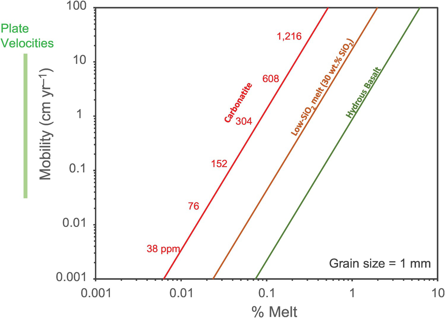
In the most depleted mantle sources containing <100 ppm CO₂, incipient melts are not mobile due to too small melt fractions (i.e. <0.02 vol.% carbonatite). In contrast, carbonatite melts formed in the most enriched mantle are very mobile (>10 cm yr^–1). Such a high mobility implies that these melts would rapidly migrate and would hardly be preserved if in physical contact with their source. This also implies unavoidable mixing processes in the column of melting where deep incipient melts rise fast and mix with upper-mantle regions (Figures 7.2 and 7.3), where melts produced at 200 km depth would rise fast and mix with the melts produced at shallower levels. The radioactive disequilibria found in MORBs have already been interpreted considering these mixing processes,Reference Faul⁷⁴ but how they impact the highly variable CO₂/Nb ratios of MORBsReference Le Voyer, Kelley, Cottrell and Hauri¹⁵ remains unaddressed.

7.5.2 EC versus Mobility of Incipient Melts

The identification of the exact nature of the melts responsible for high EC anomalies in the mantle is critical. It would allow us to decipher whether these electrical anomalies reflect lithospheric processes, being cold and involving carbonatites, or asthenospheric processes, being warm and involving (hydrated) basalts. If the electrical anomalies result from carbonated basalt (low-SiO₂) melts, they may indicate both asthenospheric and lithospheric processes, since these melts can be stable in both domains (see Figure 7.3).

We calculate that incipient melting of a peridotite can produce an electrical anomaly (~0.1 S m^–1)Reference Naif, Key, Constable and Evans²²^, Reference Kawakatsu and Utada²³^, Reference Sarafian²⁷^, Reference Tada⁷⁵ if it contains 0.1 ± 0.04% of carbonatite melts, 0.3 ± 0.15% of carbonated basalts, or 1–6% of hydrated basalts at 1350°C and 3 GPa (Figure 7.10). Note that the calculation is only weakly dependent on temperature given the low temperature dependence of the EC of incipient melts (Figure 7.7).

Figure 7.10

Incipient melting conditions producing high EC and the corresponding melt mobility. (Top) The range of melt fraction–melt compositions producing high ECs; three curves corresponding to three values of conductivity are shown. (Bottom) The mobility of incipient melt at the melt content required to produce high EC. A minimum in melt mobility appears in the case of carbonate basalts, while carbonatites and hydrated basalts are very mobile.

The comparison of Figures 7.3 and 7.10 indicates that electrical anomalies in a young plate (<10 Ma) at ~80 km depthReference Kawakatsu and Utada²³ can reasonably be matched with hydrated basalts,Reference Ni, Keppler and Behrens⁶² while deeper anomalies observed beneath older plates (i.e. >50 Ma)Reference Kawakatsu and Utada²³^, Reference Tada⁷⁵ may match any kind of CO₂-rich melt.Reference Sifré³³

The mobility of melts produced during incipient melting conditions matching a conductivity of 0.1 S m^–1 are reported in Figure 7.10. Both carbonatite and the hydrated basalt cases yield the highest velocities, favoring melt extraction, while carbonated basalts (low-SiO₂ melts) yield minimum velocities, favoring melt stability. Whether melts can be stabilized and detected by geophysical means therefore depends on the convection velocity of the mantle sourcing the melts. Highly mobile melts such as >0.1 vol.% carbonatite or 3 vol.% basalts can be detected in settings with mantle velocities of ~10 cm yr^–1 or more (e.g. the center of mantle plumes feeding volcanic hotspots such as HawaiReference Ballmer, Ito, van Hunen and Tackley⁷⁶ or the East Pacific RiseReference Kawakatsu and Utada²³^, Reference Evans⁷⁷).

Away from these extreme geodynamic settings, many types of convections can occur in the mantle at rates in the range 0.1–1.0 cm yr^–1.Reference Morency, Doin and Dumoulin¹⁶^, Reference Ballmer, van Hunen, Ito, Tackley and Bianco¹⁷^, Reference Keller and Katz¹⁹ There, the most likely type of incipient melts producing high conductivity are carbonated basalts. These melts contain 30–40 wt.% SiO₂, implying that their viscosity is close to that of basalt but with enhanced EC, as their CO₂ contents are ~10–20 wt.%. About 0.3 ± 0.15% of such melts are required to produce high EC. This corresponds to 180–440 ppm CO₂ in the mantle. Notably, these melts resemble petit-spot volcanism.Reference Hirano¹¹^, Reference Okumura and Hirano⁷⁸ These CO₂-rich melts are believed to remain in the mantle beneath plates and to be extracted when particular stress regimes just ahead of subduction zones trigger diking at a lithospheric scale.Reference Hirano¹¹

7.6 Conclusions

Due to the presence of small amounts of CO₂ and H₂O in Earth’s mantle, incipient melting can occur in the regions close to the LAB. The produced melts have unconventional physical properties such as low densities, low viscosities, high diffusion rates, and high ECs, but there are strong interplays between the chemical compositions and physical properties of these melts. In a melting column (e.g., in ridges (Figure 7.2) or intraplates (Figure 7.3)), the structural composition of the produced incipient melts greatly changes from ionic to polymerized as a function of depth. This must cause a series of extraction–accumulation processes, so far unidentified, which are critical in our interpretation the geophysical and geochemical fingerprints of magmatism. Notably, these incipient melts remain interconnected even at very small melt fractions. This implies that a broad distribution of interconnected incipient melts can impact geophysical observations. On the other hand, interconnected low-viscosity melts also mean high melt mobility, which speaks against their stability within their source regions. In particular, for the incipient melting conditions capable of producing geophysical anomalies, melt extraction must occur rapidly at a geological scale. Production–extraction of incipient melts must therefore be considered altogether within the convective mantle.

7.6.1 LAB versus Geophysical Discontinuities

The LAB is a concept assuming that Earth’s upper mantle is composed of two layers: the lower one, the asthenosphere, being adiabatic (convection controls heat transport); and the upper one, the lithosphere, being diffusive (diffusion dissipates heat). The electrical and seismic discontinuities mapped worldwide supposedly mark these boundaries, but the magmatic processes at the LAB and their geophysical visibility remain debated. The analysis provided in this chapter shows that several types of incipient melting can produce high mantle ECs. These melting processes can be lithospheric or asthenospheric, and therefore geophysical discontinuities may not image the LAB, but rather illuminate the dynamics of melting and melt transfers in the region of the LAB. Furthermore, geochemical observations have long defined the LAB as a movable boundary; that is to say, melt productions, melt infiltrations, and mantle metasomatism can cause major modifications of lithospheric roots.

Anomalous EC and regions with low seismic velocities have been mapped in many mantle region.Reference Naif, Key, Constable and Evans²²^, Reference Kawakatsu and Utada²³^, Reference Evans⁷⁷^, Reference Tada, Tarits, Baba, Utada, Kasaya and Suetsugu⁷⁹^, Reference Baba, Utada, Goto, Kasaya, Shimizu and Tada⁸⁰ A broadly distributed LVZ beneath oceanic domains is deduced from large-scale surveys,Reference Kawakatsu and Utada²³^, Reference Schmerr²⁵ but the magnitudes of the velocity decreases locally vary. Beneath cratons, no such LVZ is observed.Reference Eaton²⁶ After the Mantle ELectromagnetic and Tomography (MELT) experiment that imaged the mantle beneath the ultrafast East Pacific Rise,Reference Evans⁷⁷ several surveys have investigated quieter geodynamic settings hoping for more conventional geophysical signals, but high conductivities and low seismic velocities have often been observed.Reference Kawakatsu and Utada²³ The recently investigated NoMelt areaReference Sarafian²⁷ (70 My old oceanic plates) provides the first geophysical survey identifying no anomalous conductivity and a weak LVZ. If mantle melting is one of the ingredients causing geophysical anomalies, why does such an area exist?

7.6.2 Manifold Types of Mantle Convection Fuel Incipient Melting

The driving force of melt production is mantle convection, which produces decompression melting. There are sound geodynamic reasons to argue that decompression melting does not only occur where hot spot volcanoes pierce the surface: the inward mass transfers associated with slab sinking must be compensated by an upward flow being broadly distributed and probably more pronounced beneath oceanic basins.Reference Morency, Doin and Dumoulin¹⁶ The rate at which this upward mantle flow occurs should not exceed the melt velocities described in Figure 7.10 (i.e. ≤1 cm yr^–1), except in large plumes such as Hawaii.Reference Ballmer, Ito, van Hunen and Tackley⁷⁶ Clearly, convections, decompressions, incipient melting, and melt extractions must occur in many regions of Earth’s mantle. Convection-related decompression melting must fuel the LAB where upwelling occurs. Where mantle upwelling does not occur, a source of incipient melts simply does not exist. It is not completely clear whether this vision can explain the distribution of mantle geophysical anomalies.Reference Kawakatsu and Utada²³ Furthermore, if high EC can be explained by incipient melts, it remains unclear whether the same process could explain the low S-wave velocities in the asthenosphere.

7.7 Limits to Knowledge and Unknowns

What is the role of partial melting in the LVZ? Grain size and temperature distributions in the solid mantle may be accounted for by the LVZ,Reference Jackson and Faul⁸¹ but a recent experimental survey suggests a key role is played by incipient melting.Reference Chantel⁸² Melting is also an attractive model to account for the radial seismic anisotropyReference Kawakatsu and Utada²³ of the LVZ. Yet the classical theories of melt equilibrium distributionReference von Bargen and Waff⁶⁸ have been developed that predict that several volume percentage points of melt are required to significantly reduce seismic wave velocities.Reference Wimert and Hier-Majumder⁸³ This is at odds with recent experimental measurementsReference Chantel⁸² revealing that <1% melts drastically reduce S- and P-wave velocities.

Can the LVZ be a low-viscosity zone and can it play a role in the development of plate tectonics? The question is asked by Holtzman,Reference Holtzman⁶⁹ who tentatively responded by a “yes it can.” If minute amounts of melt can wet the mantle grain boundaries and impact large-scale geophysical properties such as EC and seismic wave velocities, they may well affect the viscosity of the mantle. If diffusion creep is the mechanism of deformation in such systems, the tremendous diffusion properties of CO₂-rich melts demand an assessment of their impact on mantle viscosity. If the LVZ is indeed a low-viscosity zone, it certainly facilitates the motion of plates as suggested by geodynamic models,Reference Höink, Jellinek and Lenardic⁸⁴ and the conjunction of there being no observed LVZ beneath cratons and the relatively slow motion of cratons in comparison to younger plates speaks to a link between the magnitude of the LVZ and the velocity of the overlying plate.

Is there a continuous process from the metasomatic rejuvenation of cratonic roots to the deployment of the LVZ?Reference Aulbach, Massuyeau and Gaillard² The chain of processes, broadly named rejuvenation, involve a combination of mechanical, thermal, chemical, and mineralogical processes.Reference Aulbach, Massuyeau and Gaillard² How does melt ascend? Certainly via a combination of dikes and porous flows, but can we fit this within a proper petrological framework? The first numerical attempts were recently conducted.Reference Keller and Katz¹⁹ Additional efforts are expected.

Acknowledgments

The authors acknowledge funding from the European Research Council (ERC project #279790), the French National Research Agency (ANR project #2010 BLAN62101), and the South African DST/NRF Research Chairs Initiative (Geometallurgy; Fanus Viljoen #64779). This is Laboratory of Excellence ClerVolc contribution 325.

Questions for the Classroom

1 What is the difference between incipient melting and partial melting of the mantle?

2 What is the nature of the produced melts and what are their physical properties?

3 What is the link between the atomic structure and the physical properties of these incipient melts?

4 Which effects could other volatile elements like S (very redox sensitive), F, Cl, and B have on the chemical–physical properties of Earth’s mantle and on the dynamics of incipient melting?

5 Why can incipient melts barely rise above 60 km, which is the depth at which the pressure is ~2 GPa?

6 What is the LAB? Can we observe it by geophysical means? What are the geophysical observables?

7 Why can or cannot the LVZ be straightforwardly attributed to partial melting?

8 Is there a unique solution to account for by high EC layers in the mantle?

9 Why can incipient melting be accounted for by EC?

10 Why are some considerations of melt mobility needed in order to interpret high mantle conductivity?

11 What is the geodynamic process that causes incipient melting?

12 Where should we then (not) observe high EC near the LAB?

References

Wallace, M.E. & Green, D.H., An experimental determination of primary carbonatite magma composition. Nature 335, 343–346 (1988).Google Scholar

Aulbach, S., Massuyeau, M., & Gaillard, F., Origins of cratonic mantle discontinuities: a view from petrology, geochemistry and thermodynamic models. Lithos 268–271, 364–382 (2017).Google Scholar

Dasgupta, R. et al., Carbon-dioxide-rich silicate melt in the Earth’s upper mantle. Nature 493, 211–215 (2013).Google Scholar

O‘Reilly, S.Y. & Griffin, W.L., The continental lithosphere–asthenosphere boundary: can we sample it? Lithos 120, 1–13 (2010).Google Scholar

Hammouda, T. & Keshav, S., Melting in the mantle in the presence of carbon: review of experiments and discussion on the origin of carbonatites. Chem. Geol. 418, 171–188 (2015).CrossRef Google Scholar

Tappe, S. et al., Craton reactivation on the Labrador Sea margins: ⁴⁰Ar/³⁹Ar age and Sr–Nd–Hf–Pb isotope constraints from alkaline and carbonatite intrusives. Earth Planet. Sci. Lett. 256, 433–454 (2007).Google Scholar

Dasgupta, R., Volatile bearing partial melts beneath oceans and continents – where, how much, and of what compositions? Am. J. Sci. 318, 141–165 (2018).Google Scholar

Coltorti, M.C. et al., Carbonatite metasomatism of the oceanic upper mantle: evidence from clinopyroxenes and glasses in ultramafic xenoliths of Grande Comore, Indian Ocean. J. Petrol. 40, 133–165 (1999).Google Scholar

Pilet, S., Baker, M.B., & Stolper, E.M., Metasomatized lithosphere and the origin of alkaline lavas. Science 320, 916–919 (2008).Google Scholar

Pinto, L.G.R. et al. Magnetotelluric deep soundings, gravity and geoid in the south São Francisco craton: geophysical indicators of cratonic lithosphere rejuvenation and crustal underplating. Earth Planet. Sci. Lett. 297, 423–434 (2010).Google Scholar

Hirano, N. et al., Volcanism in response to plate flexure. Science 313, 1426–1428 (2006).Google Scholar

Wyllie, P.J. & Huang, W.L., Carbonation and melting reactions in the system CaO–MgO–SiO₂–CO₂ at mantle pressures with geophysical and petrological applications. Contrib. Mineral. Petrol. 54, 79–107 (1976).Google Scholar

Taylor, W.R. & Green, D.H., Measurement of reduced peridotite–C–O–H solidus and implications for redox melting of the mantle. Nature 332, 349–352 (1988).Google Scholar

Stagno, V., Ojwang, D.O., McCammon, C.A., & Frost, D.J., The oxidation state of the mantle and the extraction of carbon from Earth’s interior. Nature 493, 84–88 (2013).Google Scholar

Le Voyer, M., Kelley, K.A., Cottrell, E., & Hauri, E.H., Heterogeneity in mantle carbon content from CO₂-undersaturated basalts. Nat. Commun. 8, 14062 (2017).Google Scholar

Morency, C., Doin, M.-P., & Dumoulin, C., Three-dimensional numerical simulations of mantle flow beneath mid-ocean ridges. J. Geophys. Res. Solid Earth 110, 344–356 (2005).Google Scholar

Ballmer, M.D., van Hunen, J., Ito, G., Tackley, P.J., & Bianco, T.A., Non-hotspot volcano chains originating from small-scale sublithospheric convection. Geophys. Res. Lett. 34, L23310 (2007).Google Scholar

French, S., Lekic, V., & Romanowicz, B., Waveform tomography reveals channeled flow at the base of the oceanic asthenosphere. Science 342, 227–230 (2013).Google Scholar

Keller, T. & Katz, R.F., The role of volatiles in reactive melt transport in the asthenosphere. J. Petrol. 57, 1073–1108 (2016).Google Scholar

Eggler, D.H., Does CO₂ cause partial melting in the low-velocity layer of the mantle? Geology 4, 69–72 (1976)Google Scholar

Gaillard, F. et al., Carbonatite melts and electrical conductivity in the asthenosphere. Science 322, 1363–1365 (2008).Google Scholar

Naif, S., Key, K., Constable, S., & Evans, R.L., Melt-rich channel observed at the lithosphere–asthenosphere boundary. Nature 495, 356–359 (2013).Google Scholar

Kawakatsu, H. & Utada, H., Seismic and electrical signatures of the lithosphere–asthenosphere system of the normal oceanic mantle. Ann. Rev. Earth Planet. Sci. 45, 139–167 (2017).Google Scholar

Rychert, C.A., Laske, G., Harmon, N., & Shearer, P.M., Seismic imaging of melt in a displaced Hawaiian plume. Nat. Geosci. 6, 657–660 (2013)Google Scholar

Schmerr, N., The Gutenberg discontinuity: melt at the lithosphere–asthenosphere boundary. Science 380, 1480–1483 (2012).Google Scholar

Eaton, D.W. et al., The elusive lithosphere–asthenosphere boundary (LAB) beneath cratons. Lithos 109, 1–22 (2009).Google Scholar

Sarafian, E. et al., The electrical structure of the central Pacific upper mantle constrained by the NoMelt experiment. Geochem. Geophys. Geosyst. 16, 1115–1132 (2015).CrossRef Google Scholar

Hirschmann, M., Tenner, T., Aubaud, C., & Withers, A.C., Dehydration melting of nominally anhydrous mantle: the primacy of partitioning. Phys. Earth Planet. Inter. 176, 54–68 (2009).Google Scholar

Massuyeau, M., Gardés, E., Morizet, Y., & Gaillard, F., A model for the activity of silica along the carbonatite–kimberlite–mellilitite–basanite melt compositional joint. Chem. Geol. 418, 206–216 (2015).Google Scholar

Hirschmann, M.M., Partial melt in the oceanic low velocity zone. Phys. Earth Planet. Inter. 179, 60–71 (2010).Google Scholar

McKenzie, D., Jackson, J., & Priestley, K., Thermal structure of oceanic and continental lithosphere. Earth Planet. Sci. Lett. 233, 337–349 (2005).Google Scholar

Burgos, G. et al., Oceanic lithosphere–asthenosphere boundary from surface wave dispersion data. J. Geophys. Res. Solid Earth 119, 1079–1093 (2014).Google Scholar

Sifré, D. et al., Electrical conductivity during incipient melting in the oceanic low-velocity zone. Nature 509, 81-85 (2014).Google Scholar

Mysen, B.O. & Richet, P., Silicate Glasses and Melts: Properties and Structure. Elsevier, Amsterdam (2005).Google Scholar

Jones, A.P., Genge, M., & Carmody, L., Carbonate melts and carbonatites. Rev. Mineral. Geochem. 75, 289–322 (2013).Google Scholar

Desmaele, E., Physico-chemical properties of molten carbonates by atomistic simulations. PhD thesis, Sorbonne University (2017).Google Scholar

Vuilleumier, R., Seitsonen, A., Sator, N., & Guillot, B., Structure, equation of state and transport properties of molten calcium carbonate (CaCO₃) by atomistic simulations. Geochim. Cosmochim. Acta 141, 547–566 (2014).Google Scholar

Vuilleumier, R., Seitsonen, A.P., Sator, N., & Guillot, B., Carbon dioxide in silicate melts at upper mantle conditions: insights from atomistic simulations. Chem. Geol. 418, 77–88 (2015).Google Scholar

Dufils, T., Sator, N., & Guillot, B., 2018. Properties of planetary melts by molecular dynamics simulation. Chem. Geol. 493, 298–315 (2018).Google Scholar

Guillot, B. & Sator, N., Carbon dioxide in silicate melts: a molecular dynamics simulation study. Geochim. Cosmochim. Acta 75, 1829–1857 (2011).Google Scholar

Moussallam, Y. et al., The molecular structure of melts along the carbonatite–kimberlite–basalt compositional joint: CO₂ and polymerisation. Earth Planet. Sci. Lett. 434, 129–140 (2016).Google Scholar

Morizet, Y., Florian, P., Paris, M., & Gaillard, F., ¹⁷O NMR evidence of free ionic clusters Mn⁺ CO₃^2– in silicate glasses: precursors for carbonate–silicate liquids immiscibility. Am. Mineral. 102, 1561–1564 (2017)Google Scholar

Brooker, R.A. & Kjarsgaard, B.A., Silicate–carbonate liquid immiscibility and phase relations in the system SiO₂–Na₂O–Al₂O₃–CaO–CO₂ at 0.1–2.5 GPa with applications to carbonatite genesis. J. Petrol. 52, 1281–1305 (2011).Google Scholar

Novella, D. et al. Melting phase relations of model carbonated peridotite from 2 to 3 GPa in the system CaO–MgO–Al₂O₃–SiO₂–CO₂ and further indication of possible unmixing between carbonatite and silicate liquids. J. Geophys. Res. Solid Earth 119, 2780–2800 (2014).Google Scholar

Morizet, Y. et al., Towards the reconciliation of viscosity change and CO₂-induced polymerization in silicate melts. Chem. Geol. 458, 38–47 (2017).CrossRef Google Scholar

Liu, Q. & Lange, R.A., New density measurements on carbonate liquids and the partial molar volume of the CaCO₃ component. Contrib. Mineral. Petrol. 146, 370–381 (2003).CrossRef Google Scholar

Bouhifd, M.A., Whittington, A.G., & Richet, P., Densities and volumes of hydrous silicate melts: new measurements and predictions. Chem. Geol. 418, 40–50 (2015).Google Scholar

Jing, Z. & Karato, S., Compositional effect on the pressure derivatives of bulk modulus of silicate melts. Earth Planet. Sci. Lett. 272, 429–436 (2008).Google Scholar

Sakamaki, T., Density of hydrous magma. Chem. Geol. 475, 135–139 (2017).Google Scholar

Ghosh, S. et al., Stability of carbonated magmas at the base of the Earth’s upper mantle. Geophys. Res. Lett. 34, L22312 (2007).Google Scholar

Sakamaki, T. et al., Density of carbonated peridotite magma at high pressure using an X-ray absorption method. Am. Mineral. 96, 553–557 (2011).Google Scholar

Duncan, M.S. & Agee, C.B., The partial molar volume of carbon dioxide in peridotite partial melt at high pressure; Earth Planet. Sci. Lett. 312, 429–436 (2011).Google Scholar

Ghosh, D.B., Bajgain, S.K., Mookherjee, M., & Karki, B.B. Carbon-bearing silicate melt at deep mantle conditions. Sci. Rep. 7, 1–5 (2017).Google Scholar

Genge, M.J., Price, G.D., & Jones, A.P. Molecular dynamics simulations of CaCO₃ melts to mantle pressures and temperatures: implications for carbonatite magmas. Earth Planet. Sci. Lett. 131, 225–238 (1995).Google Scholar

Dobson, D.P. et al., In-situ measurement of viscosity and density of carbonate melts at high pressure. Earth Planet. Sci. Lett. 143, 207–215 (1996).Google Scholar

Kono, Y. et al., Ultralow viscosity of carbonate melts at high pressures. Nature Commun. 5, 5091 (2014).Google Scholar

Sifré, D., Hashim, L., & Gaillard, F., Effects of temperature, pressure and chemical compositions on the electrical conductivity of carbonated melts and its relationship with viscosity. Chem. Geol. 418, 189–197 (2015).Google Scholar

Hammouda, T. & Laporte, D., Ultrafast mantle impregnation by carbonatite melts. Geology 28, 283–285 (2000).Google Scholar

Sakamaki, T. et al., Ponded melt at the boundary between the lithosphere and asthenosphere. Nat. Geosci. 6, 1041–1044 (2013).Google Scholar

Karato, S., The role of hydrogen in the electrical conductivity of the upper mantle. Nature 347, 272–273 (1990).Google Scholar

Gardés, E., Gaillard, F., & Tarits, P., Comment to “High and highly anisotropic electrical conductivity of the asthenosphere due to hydrogen diffusion in olivine” by Dai and Karato [Earth Planet. Sci. Lett. 408 (2014) 79–86]. Earth Planet. Sci. Lett. 427, 296–299, (2015).Google Scholar

Ni, H., Keppler, H., & Behrens, H., Electrical conductivity of hydrous basaltic melts: implications for partial melting in the upper mantle. Contrib. Mineral. Petrol. 162, 637–650 (2011).Google Scholar

Yoshino, T., Laumonier, M., McIsaac, E., & Katsura, T., Electrical conductivity of basaltic and carbonatite melt-bearing peridotites at high pressures: implications for melt distribution and melt fraction in the upper mantle. Earth Planet. Sci. Lett. 295, 593–602 (2010)Google Scholar

Yoshino, T. et al., Electrical conductivity of partial molten carbonate peridotite. Phys. Earth Planet. Inter. 194–195, 1–9 (2012).Google Scholar

Yoshino, T., Gruber, B., & Reinier, C., Effects of pressure and water on electrical conductivity of carbonate melt with implications for conductivity anomaly in continental mantle lithosphere. Phys. Earth Planet. Inter. 281, 8–16 (2018)Google Scholar

Hunter, R.H. & McKenzie, D., The equilibrium geometry of carbonate melts in rocks of mantle composition. Earth Planet. Sci. Lett. 92, 347–356 (1989).Google Scholar

Watson, E.B., Brenan, J.M., & Baker, D.R., Distribution of fluids in the continental mantle, in Menzies, M.A., ed., Continental Mantle: Oxford Monographs on Geology and Geophysics. Oxford University Press, Oxford, 111–125 (1990).Google Scholar

von Bargen, N. & Waff, H.S., Permeabilities, interfacial areas and curvatures of partially molten systems: results of numerical computations of equilibrium microstructures. J. Geophys. Res. 91, 9261–9276 (1986).Google Scholar

Holtzman, B.K., Questions on the existence, persistence, and mechanical effects of a very small melt fraction in the asthenosphere, Geochem. Geophys. Geosyst. 17, 470–484 (2016).Google Scholar

Minarik, W.G. & Watson, E.B., Interconnectivity of carbonate melt at low melt fraction. Earth Planet. Sci. Lett. 133, 423–437 (1995).Google Scholar

Laumonier, M. et al., Experimental determination of melt interconnectivity and electrical conductivity in the upper mantle. Earth Planet. Sci. Lett. 463, 286–297 (2017).Google Scholar

Mu, S. & Faul, U.H., Grain boundary wetness of partially molten dunite. Contrib. Mineral. Petrol. 171, 40 (2016).Google Scholar

Miller, K.J., Montési, L.G.J., & Zhu, W-l., Estimates of olivine–basaltic melt electrical conductivity using a digital rock physics approach. Earth Planet. Sci. Lett. 432, 332–341 (2015).Google Scholar

Faul, U., Melt retention and segregation beneath mid-ocean ridges. Nature 410, 920–923 (2001).Google Scholar

Tada, N. et al., Electromagnetic evidence for volatile-rich upwelling beneath the society hotspot, French Polynesia. Geophys. Res. Lett. 43, 12021–12026 (2016).Google Scholar

Ballmer, M.D., Ito, G., van Hunen, J., & Tackley, P.J., Spatial and temporal variability in Hawaiian hotspot volcanism induced by small-scale convection. Nat. Geosci. 4, 457–460 (2011).Google Scholar

Evans, R.L. et al., Geophysical controls from the MELT area for compositional controls on oceanic plates, Nature 437, 249–252 (2005).Google Scholar

Okumura, S. & Hirano, N., Carbon dioxide emission to Earth’s surface by deep-sea volcanism. Geology 41, 1167–1170 (2013).Google Scholar

Tada, N., Tarits, P., Baba, K., Utada, H., Kasaya, T., & Suetsugu, D., Electromagnetic evidence for volatile-rich upwelling beneath the society hotspot, French Polynesia. Geophys. Res. Lett. 43, 12021–12026 (2016).Google Scholar

Baba, K., Utada, H., Goto, T.-N., Kasaya, T., Shimizu, H., & Tada, N., Electrical conductivity imaging of the Philippine Sea upper mantle using seafloor magnetotelluric data. Phys. Earth Planet. Inter. 183, 44–62 (2010).Google Scholar

Jackson, I. & Faul, U.H., Grain size-sensitive viscoelastic relaxation in olivine: towards a robust laboratory-based model for seismological application. Phys. Earth Planet. Inter. 183, 151–163 (2010).Google Scholar

Chantel, J. et al., Experimental evidence supports mantle partial melting in the asthenosphere. Sci. Adv. 2, e1600246 (2016).Google Scholar

Wimert, J. & Hier-Majumder, S., A three-dimensional microgeodynamic model of melt geometry in the Earth’s deep interior. J. Geophys. Res. 117, B04203 (2012).Google Scholar

Höink, T., Jellinek, A.M., & Lenardic, A. Viscous coupling at the lithosphere–asthenosphere boundary. Geochem. Geophys. Geosyst. 12, Q0AK02 (2011).Google Scholar

Gardés, E., Gaillard, F., & Tarits, P., Toward a unified hydrous olivine electrical conductivity law. Geochem. Geophys. Geosyst. 15, 4984–5000 (2014).Google Scholar

Figure 7.1 Pressure–temperature plot showing the stability fields for different types of mantle melt as a function of the volatile contents. Different geotherms (10 My, 80 My, cratons) are superimposed. The CO2-bearing hydrous peridotite solidus is calculated from the combination of solidus temperatures of Ref. 1 from 0 to ~4 GPa and Ref. 13 at higher pressures. We connected the melting curve of CO2-bearing hydrous peridotite to that of the dehydration solidus of nominally anhydrous peridotite28 (considering peridotite with 460 ppm H2O) at low pressures.

Figure 7.2 Melt composition (left) and melt fraction (right) produced during adiabatic mantle melting (temperature = 1360°C or 1480°C when specified). Under most of the pressure–temperature–volatile content conditions shown here, incipient melting occurs. Incipient melting of depleted (100 ppm H2O–100 ppm CO2) to enriched (500 ppm) mantle sources is considered. The stars show compositions for which viscosities were determined by molecular dynamics (see Section 7.3).

Figure 7.3 Profiles of melt compositions in intraplate geodynamic settings of variable ages (cratons, 80 Ma, and 10 Ma from left to right) compared to the depth range of the Gutenberg discontinuity (G) and the LVZ. The curve labeled “LAB” corresponds to the thermal lithosphere–asthenosphere boundary. The LAB displays a depth that changes with the age of the plate.31 One sees that the degree of H2O–CO2 enrichment moderately affects the type of melt composition formed at lithospheric depth. It is essentially the temperature change with depth that controls the melt composition. This narrow range of lithospheric melt compositions is at odds with the large range of melt compositions that are formed in the convective mantle, which strongly depends on the degree of H2O–CO2 enrichment, as shown in Figure 7.2.

Figure 7.4 MD-generated snapshots of a carbo-silicate melt (17 wt.% SiO2 and 28 wt.% CO2) at 8 GPa and 1727 K. In the left panel, all atoms are depicted (SiO4 in yellow and red, CO3 in cyan and red, Mg in green, Ca in cyan, Na in blue, K in pink, and Fe in purple, with Al and Ti not being represented for clarity reasons). In the middle panel, the carbonate ions are not depicted in order to show the silicate network, whereas in the right panel, the SiO4 units are not depicted in order to better visualize the arrangement of the carbonated component of the melt. It is clear that the SiO4 and CO3 ions do not mix well and form two subnetworks. A movie of the MD simulation may be found in the supplementary online material.

Figure 7.5 Effects of H2O and CO2 on the melt density curve as a function of pressure. (a) Calculations of melt density are performed for the melts produced along the adiabatic path of Figure 7.2. The black dots correspond to the chemical compositions marked by stars in Figure 7.2. Open symbols are H2O free and full symbols contain both CO2 and H2O. Values along the line “melt + CO2” indicate the CO2 content in wt.%, and those along the line “melt + CO2 + H2O” indicate the CO2 content (first number) in wt.% and the H2O content (second number) in wt.%. The effects of H2O content on the compressibility curve of a basaltic melt (red) and a CO2-free kimberlitic melt (blue) are given for comparison. (b) The evolution of the partial molar volumes of CO2 and H2O as a function of pressure at 2000 K as given by the Vinet equation of state for CO251 and for H2O.49 Notice that these partial molar volumes are independent of the melt composition. The temperature dependence of VCO2 is negligible in the range 1673–2000 K.

Figure 7.6 Viscosity changes as a function of melt silica content in dry carbonated melts (left) and as a function of H2O content in CO2-free melts (right). The conditions of calculation are 1400–1450°C and 2–8 GPa. Left: the melt compositions change from carbonatite (0 wt.% SiO2) to basalt (45 wt.% SiO2); both MD calculations (this work) and experimental measurements56 are shown. Right: the effect of water on the viscosity of silicate melts; basaltic, peridotitic, and kimberlitic melts are similarly affected by water. MORB = mid-ocean ridge basalt.

Figure 7.7 The EC of incipient melts either pure (left) or embedded into a olivine matrix (right). (Left) Basalts, kimberlites, and carbonatites are shown. The basalts are labeled in terms of water contents.62 The kimberlite are labeled in terms of CO2.33,63,64 Carbonatite melts are compiled from Refs. 33, 57, 65. (Right) The conductivity of the mantle during incipient melting. The four cases from Figure 7.2 are converted here into EC versus depth signals. The solid mantle is approximated by hydrated olivine using the model of hydrated olivine.85 The melt conductivity is calculated from Ref. 33. Values of 0.1 S m–1 are identified by the magnetotelluric community as anomalies.

Figure 7.8 Evidence for interconnectivity at small melt fractions within olivine aggregates. (Left) Bulk EC of a carbonated melt/olivine mixture, evidencing melt interconnection over the range of investigated melt fractions down to 0.7 vol.%. Experimental data63 (blue circles) were collected at 1377°C and 3 GPa. The HS+ mixing model (7.4) does reproduce the data very well, while the tube mixing model (7.5) appears inappropriate. Models were calculated (no adjustments) using σmelt = 8.91 × 101 S m–1 (conductivity at 100% melt) and σsolid = 9.23 × 10–3 S m–1 (olivine conductivity at 1377°C).85 (Right) Bulk diffusivity of iron in a carbonated melt/olivine mixture evidencing melt interconnection down to very small melt fractions <0.01 vol.%. Experimental data70 were obtained at 1300°C and 1 GPa. Runs with longest durations (95–127 hours, empty blue circles) are differentiated from the other runs (5–49 hours, full blue circles), since they were possibly affected by melt loss (see text). Data roughly follow a trend that is intermediate between the bulk diffusivities of pure molten carbonate/olivine mixture and of a CO2-free molten silicate/olivine mixture (dashed curves). The gap at ~0.07 vol.% melt, if significant, might mark a transition from tube to HS+ types of interconnection. The dashed curves are HS+ mixing laws with Dmelt = 1.8 × 10–9 m2 s–1 for pure a molten carbonate/olivine mixture37 (diffusivity of Ca in CaCO3 at 1300°C and 1 GPa) and Dmelt = 1.3 × 10–11 m2 s–1 for a CO2-free molten silicate/olivine mixture (diffusivity of Fe in basaltic melt at 1300°C and 1 atm), where the diffusivity in a melt-free solid matrix is given by runs with no added carbonate,70 Dsolid = 3.45 × 10–15 m2 s–1. The blue curve is an adjustment of the experimental data with a HS+ mixing law. The added carbonate weight fractions reported by Ref. 70 were converted to the melt volume fractions using conversion factors of ~1.5.

Figure 7.9 The melt vertical velocity at mantle depth versus melt fractions during incipient melting. Carbonatites, carbonated basalts, and hydrated basalts are shown. Carbonatites (containing 40 wt.% CO2) are labeled in equivalent ppm CO2 contents in the bulk rock. This concentration range covers depleted to enriched MORB sources.15 The basalt contains 2 wt.% H2O and 0.2 wt.% CO2, while the carbonated basalt contains 2 wt.% H2O and 15 wt.% CO2.

Figure 7.10 Incipient melting conditions producing high EC and the corresponding melt mobility. (Top) The range of melt fraction–melt compositions producing high ECs; three curves corresponding to three values of conductivity are shown. (Bottom) The mobility of incipient melt at the melt content required to produce high EC. A minimum in melt mobility appears in the case of carbonate basalts, while carbonatites and hydrated basalts are very mobile.

Accessibility standard: Unknown

Why this information is here

This section outlines the accessibility features of this content - including support for screen readers, full keyboard navigation and high-contrast display options. This may not be relevant for you.

Accessibility Information

Accessibility compliance for the HTML of this chapter is currently unknown and may be updated in the future.