


1. Introduction
The Indian summer monsoon (ISM) exerts significant societal and economic influences on billions of people in Asia. Climatologically, ISM was thought to be induced by seasonal thermal contrast between the Asian continent and the Indian Ocean (IO) (Webster et al. Reference Webster, Magana, Palmer, Shukla, Tomas, Yanai and Yasunari1998; Wang et al. Reference Wang, Clemens, Beaufort, Braconnot, Ganssen, Jian and Sarnthein2005; Wu GX et al. Reference Wu, Liu, He, Bao, Duan and Jin2012), but synoptically was argued as a result of the seasonal shift of Intertropical Convergence Zone (Gadgil, Reference Gadgil2003, Reference Gadgil2018; Geen et al. Reference Geen, Bordoni, Battisti and Hui2020; Yang et al. Reference Yang, Zhang, Yi, Zhong, Lu, Wan, Du and Xiang2023), or a result of moisture or latent heat export from the tropical Indian Ocean (TIO) (Behera et al. Reference Behera, Krishnan and Yamagata1999; Bolton et al. Reference Bolton, Chang, Clemens, Kodama, Ikehara, Medina-Elizalde, Paterson, Roberts, Rohling, Yamamoto and Zhao2013; Clemens et al. Reference Clemens, Yamamoto, Thirumalai, Giosan, Richey, Nilsson-Kerr, Rosenthal, Anand and McGrath2021). On seasonal to interannual scales, the forecast skill of ISM largely relies on tropical air–sea coupled climate modes, such as the El Niño-Southern Oscillation (ENSO) and the Indian Ocean Dipole (IOD) (Webster & Yang, Reference Webster and Yang1992; Saji et al. Reference Saji, Goswami, Vinayachandran and Yamagata1999; Ashok et al. Reference Ashok, Guan and Yamagata2001; Fasullo & Webster, Reference Fasullo and Webster2002; Gadgil et al. Reference Gadgil, Vinayachandran and Francis2003, Reference Gadgil, Rajeevan and Francis2007; Krishnan et al. Reference Krishnan, Ramesh, Samala, Meyers, Slingo and Fennessy2006, Reference Krishnan, Sundaram, Sundaram, Swapna, Kumar, Kumar, Ayantika and Mujumdar2011; Ashok & Saji, Reference Ashok and Saji2007; Wang et al. Reference Wang, Liu, Kim, Webster, Yim and Xiang2013).
For people inhabiting monsoon regions, seasonal variations of the rainfall are more important than wind anomalies. Traditionally, increased ISM rainfall (ISMR) was attributed to La Niña events or positive IOD events (Ashok et al. Reference Ashok, Guan, Saji and Yamagata2004). But modern observed relationships among ENSO, IOD, and ISMR are not stationary and depend on some other factors such as the flavor of ENSO (Kumar et al. Reference Kumar, Rajagopalan and Cane1999, Reference Kumar, Rajagopalan, Hoerling, Bates and Cane2006; Ashok et al. Reference Ashok, Behera, Rao, Weng and Yamagata2007), and the interplay of ENSO and IOD (Ashok et al. Reference Ashok, Guan and Yamagata2001, Reference Ashok, Guan, Saji and Yamagata2004; Gadgil et al. Reference Gadgil, Vinaychandran, Francis and Gadgil2004, Reference Gadgil, Rajeevan and Francis2007; Ashok & Saji, Reference Ashok and Saji2007; Ihara et al. Reference Ihara, Kushnir, Cane and De la Peña2007; Li et al. Reference Li, Cai and Lin2016). Due to the concurrence of La Niña and negative IOD (or El Niño and positive IOD), the effect of IOD on ISMR tends to cancel that of ENSO (depending on the phases and strengths of two modes) (Ashok et al. Reference Ashok, Guan and Yamagata2001; Gadgil et al. Reference Gadgil, Vinaychandran, Francis and Gadgil2004). Thus, ENSO itself explains only 30% of the interannual variability of ISMR in observations (Gadgil, Reference Gadgil2014), and atmospheric general circulation models (AGCMs) with ENSO-related sea surface temperature (SST) as boundary conditions have poor skill of simulation of ISMR variations (Gadgil et al. Reference Gadgil, Rajeevan and Francis2007; Gadgil & Srinivasan, Reference Gadgil and Srinivasan2011). This indicates the tenuousness of relying on ENSO for ISMR predictions (Pottapinjara et al. Reference Pottapinjara, Girishkumar, Sivareddy, Ravichandran and Murtugudde2016). Fortunately, Krishnan et al. (Reference Krishnan, Sundaram, Sundaram, Swapna, Kumar, Kumar, Ayantika and Mujumdar2011) found that if AGCMs were coupled to a slab-ocean model with varied mixed-layer depth in TIO, then the model could correctly simulate the observed ISMR changes during positive IOD events. It means that we can further improve the forecast skill of ISMR by considering air–sea coupling (Kumar et al. Reference Kumar, Hoerling and Rajagopalan2005), or directly accounting for oceanic moisture and latent heat supplement of ISMR in the TIO (Behera et al. Reference Behera, Krishnan and Yamagata1999; Krishnan et al. Reference Krishnan, Ramesh, Samala, Meyers, Slingo and Fennessy2006).
From an energetic viewpoint, the ocean is the largest heat capacitor of the earth’s climate system and a main source of atmospheric moist static energy (MSE). While the summer monsoon transports huge water vapor and latent heat from tropical oceans into continents (Trenberth et al. Reference Trenberth, Stepaniak and Caron2000; Fasullo & Trenberth, Reference Fasullo and Trenberth2008; Trenberth & Fasullo, Reference Trenberth and Fasullo2013; Wang et al. Reference Wang, Wang, Cheng, Fasullo, Guo, Kiefer and Liu2014, Reference Wang, Wang, Cheng, Fasullo, Guo, Kiefer and Liu2017; Biasutti et al. Reference Biasutti, Voigt, Boos, Braconnot, Hargreaves, Harrison, Kang, Mapes, Scheff, Schumacher, Sobel and Xie2018), it has been proved to be greatly modulated by heat storage or transport anomalies in tropical oceans across different time scales (Jalihal et al. Reference Jalihal, Bosmans, Srinivasan and Chakraborty2019a, Reference Jalihal, Srinivasan and Chakraborty2019b; Lutsko et al. Reference Lutsko, Marshall and Green2019; Yang YP et al. Reference Yang, Xiang, Zhang, Zhong and Zhang2019). Since the ocean thermal energy required for fueling monsoon circulations comes from the upper ocean rather than the sea surface, upper ocean heat content (OHC) changes in the tropics can be taken as the heat engine of global monsoon (Cheng et al. Reference Cheng, Trenberth, Fasullo, Boyer, Abraham and Zhu2017, Reference Cheng, von Schuckmann, Abraham, Trenberth, Mann, Zanna, England, Zika, Fasullo, Yu, Pan, Zhu, Newsom, Bronselaer and Lin2022; Hill, Reference Hill2019; Jian et al. Reference Jian, Wang, Dang, Mohtadi, Rosenthal, Lea, Liu, Jin, Ye, Kuhnt and Wang2022).
At modern seasonal or interannual scales, upper OHC anomalies associated with ENSO or ENSO-like conditions in the tropical Pacific or Atlantic oceans have been proposed as precursors of ISMR (Rajeevan & McPhaden, Reference Rajeevan and McPhaden2004; Rajeevan & Pai, Reference Rajeevan and Pai2007; Pottapinjara et al. Reference Pottapinjara, Girishkumar, Sivareddy, Ravichandran and Murtugudde2016). But recent observations suggest that (Ali et al. Reference Ali, Nagamani, Sharma, Gopal, Rajeevan, Goni and Bourassa2015; Venugopal et al. Reference Venugopal, Ali, Bourassa, Zheng, Goni, Foltz and Rajeevan2018), at least from the year 1993 to 2017 AD, the mixed layer OHC or mean temperature above 26°C in the southwest TIO during boreal winter–spring is a better qualitative predictor of ISMR than those Pacific ENSO indexes. This may be explained by the Indo-Pacific Ocean Capacitor effect (IPOC) (Xie et al. Reference Xie, Annamalai, Schott and McCreary2002, Reference Xie, Hu, Hafner, Tokinaga, Du, Huang and Sampe2009, Reference Xie, Kosaka, Du, Hu, Chowdary and Huang2016; Du et al. Reference Du, Xie, Huang and Hu2009, Reference Du, Yang and Xie2011): El Niño events can induce anomalous atmospheric downward motions and easterlies in the eastern TIO (EIO), and associated ocean wave dynamics will increase the upper OHC in the western TIO (WIO) during the following winter. After multiple air–sea coupled feedbacks, warmer SST emerges in the northern IO (NIO) and anomalous atmospheric anticyclonic circulation (AAC) extends from the Northwest Pacific to the Bay of Bengal (BOB) during boreal summer. While the surface easterlies south of the AAC greatly suppress the ISM westerlies, the warmer NIO was argued to have provided more evaporated moisture for the increased ISM rainfall over western and southern India (Mishra et al. Reference Mishra, Smoliak, Lettenmaier and Wallace2012; Xie et al. Reference Xie, Kosaka, Du, Hu, Chowdary and Huang2016; Darshana et al. Reference Darshana, Chowdary, Gnanaseelan, Parekh and Srinivas2020).
It should be noted that IPOC-associated winter OHC anomalies may be also triggered by positive IOD events (Chen et al. Reference Chen, Li, Du, Wen, Wu and Xie2021; Du et al. Reference Du, Chen, Xie, Zhang, Zhang and Cai2022, Reference Du, Wang, Wang, Liu, Liang, Zhang, Chen, Liu, Wu, Yu and Zhang2023). And the summer OHC seesaw along the equatorial IO (with warmer WIO and cooler EIO) itself is a robust index of IOD development (McPhaden & Nagura Reference McPhaden and Nagura2013). Although many studies have emphasized the role of a cooler EIO on the increased ISMR from intraseasonal to interannual time scales (Ashok et al. Reference Ashok, Guan, Saji and Yamagata2004; Krishnan et al. Reference Krishnan, Ramesh, Samala, Meyers, Slingo and Fennessy2006, Reference Krishnan, Sundaram, Sundaram, Swapna, Kumar, Kumar, Ayantika and Mujumdar2011), the long-term relationships among IOD, TIO OHC, and ISMR are still unclear either in historical periods or in geological periods.
In this study, we first distinguished those air–sea coupled changes related to ISMR from those related to ISM wind and highlighted the role of IOD-associated OHC (especially in WIO) on ISMR by analyzing reanalysis datasets across the 20th century. Then from a paleoclimatic perspective, we explored the relations of TIO OHC anomalies and ISMR at the 23,000 years’ precessional time scales, based on simulations of air–sea coupled model (and its atmospheric component) under orbital insolation and GHG forcings. Despite different time scales and external forcings, both modern observation and paleoclimate simulation suggest a significant modulation of summer positive IOD-like OHC pattern on ISMR.
2. Data, models, and methods
2.a. Modern observations
Atmospheric variables (such as surface pressure, 850 hPa wind fields, rainfall) come from the monthly mean NOAA-CIRES-DOE 20th Century Reanalysis version 3 (20CRv3) of 1º resolution spanning from the year 1836 to 2015 AD (Slivinski et al. Reference Slivinski, Compo, Whitaker, Sardeshmukh, Giese, McColl, Allan, Yin, Vose, Titchner, Kennedy, Spencer, Ashcroft, Brönnimann, Brunet, Camuffo, Cornes, Cram, Crouthamel, Dominguez-Castro, Freeman, Gergis, Hawkins, Jones, Jourdain, Kaplan, Kubota, Blancq, Lee, Lorrey, Luterbacher, Maugeri, Mock, Moore, Przybylak, Pudmenzky, Reason, Slonosky, Smith, Tinz, Trewin, Valente, Wang, Wilkinson, Wood and Wyszyński2019, Reference Slivinski, Compo, Sardeshmukh, Whitaker, McColl, Allan, Brohan, Yin, Smith, Spencer, Vose, Rohrer, Conroy, Schuster, Kennedy, Ashcroft, Brönnimann, Brunet, Camuffo, Cornes, Cram, Dominguez-Castro, Freeman, Gergis, Hawkins, Jones, Kubota, Lee, Lorrey, Luterbacher, Mock, Przybylak, Pudmenzky, Slonosky, Tinz, Trewin, Wang, Wilkinson, Wood and Wyszyński2021) (https://psl.noaa.gov/data/gridded/data.20thC_ReanV3.html). Ocean temperature used for calculating OHC comes from the monthly mean Simple Ocean Data Assimilation (SODA) reanalysis dataset (version 2.2.4) with 0.5º horizontal resolution and vertical 40 layers spanning from the year 1871 to 2010 AD (Carton et al. Reference Carton, Seidel and Giese2012) (https://apdrc.soest.hawaii.edu/datadoc/soda_2.2.4.php). The upper OHC above 26°C (OHC26, Joules m-2) is calculated according to the following equation (Pu et al. Reference Pu, Yu, Hu and Chen2003; Yang XX et al. Reference Yang, Wu, Liu and Yuan2019):
 $$OHC = \mathop \int \nolimits_z^0 C_p*\rho *T*dz = C_p*\mathop \sum \nolimits_{i = 1}^n ({\rho _i}*{T_i}*d{Z_i})$$
Here, Cp is the heat capacity of sea water taken as 4178 J kg−1 °C−1, ρ is potential density, T is ocean temperature, z is the depth of 26°C isotherm, n is the total layers from surface to the depth z, and ρ i, Ti, dZi are density, temperature, and layer thickness for the layer i. The regional averaged January–February–March (JFM) OHC26 over the western Indian Ocean (WIO, 5º S-15º N, 40º E-60º E) is named as OHC26_WIO.
According to Li & Zeng (Reference Li and Zeng2002), the ISM wind intensity is defined as June–July–August–September (JJAS) averaged Dynamical Normalized Seasonality (DNS) index of 850 hPa winds within the South Asian domain (5º N-22.5º N, 35º E-97.5º E), calculated using the 20CRv3 reanalysis dataset. The ISMR is defined as the area-weighted average of the JJAS rainfall of all the 36 meteorological subdivisions in India during the time period 1871–2016 (Kothawale et al. Reference Kothawale and Rajeevan2017) (downloaded from https://tropmet.res.in/static_pages.php?page_id=53). For the intensity of IOD and ENSO, we use the Dipole Mode Index (DMI) (Saji et al. Reference Saji, Goswami, Vinayachandran and Yamagata1999) and the Southern Oscillation Index (SOI) (Ropelewski & Jones, Reference Ropelewski and Jones1987) from NOAA Physical Sciences Laboratory (PSL) website (https://psl.noaa.gov/gcos_wgsp/Timeseries). Here, DMI was calculated as August–September–October (ASO) mean time series and to resolve the seasonal evolution of ENSO–ISMR relationship (Wu RG et al. Reference Wu, Chen and Chen2012; Chakraborty, Reference Chakraborty2018), SOI was calculated as June–July–August (JJA) mean and December–January-February (DJF) mean time series (called SOIJJA and SOIDJF), respectively.
In Figure 1, the lead-lag cross correlation (R) of two time series was calculated using the Past software (version 4.03) (Hammer et al. Reference Hammer, Harper and Ryan2001). Given that ISMR and OHC26 are both influenced by multiple parameters, we do not expect there to be an extremely good correlation between a single parameter and ISMR (or OHC26_WIO). We also do not attempt to quantitatively predict ISMR using other parameters, but only qualitatively illustrate the linkage among ENSO, IOD, OHC, and ISMR at interannual time scale. Considering that this relationship may be not stationary, the 20-year moving correlation of two time series was calculated using the Matlab program written by David De Vleeschouwer (De Vleeschouwer, Reference De Vleeschouwer2010). In Figures 2 and 3, linear regression analysis was conducted for different variables (such as surface pressure, 850 hPa wind fields, rainfall, OHC26) against the normalized time series of a specific index (i.e., DNS, ISMR, SOI, DMI, and OHC26_WIO), using the NCAR Command Language (version 6.6.2). Monthly mean SST in TIO were also regressed onto the normalized DMI index for further sensitivity experiments (see section 2.c), and their JFM and July–August–September (JAS) means are shown in Figure 4.
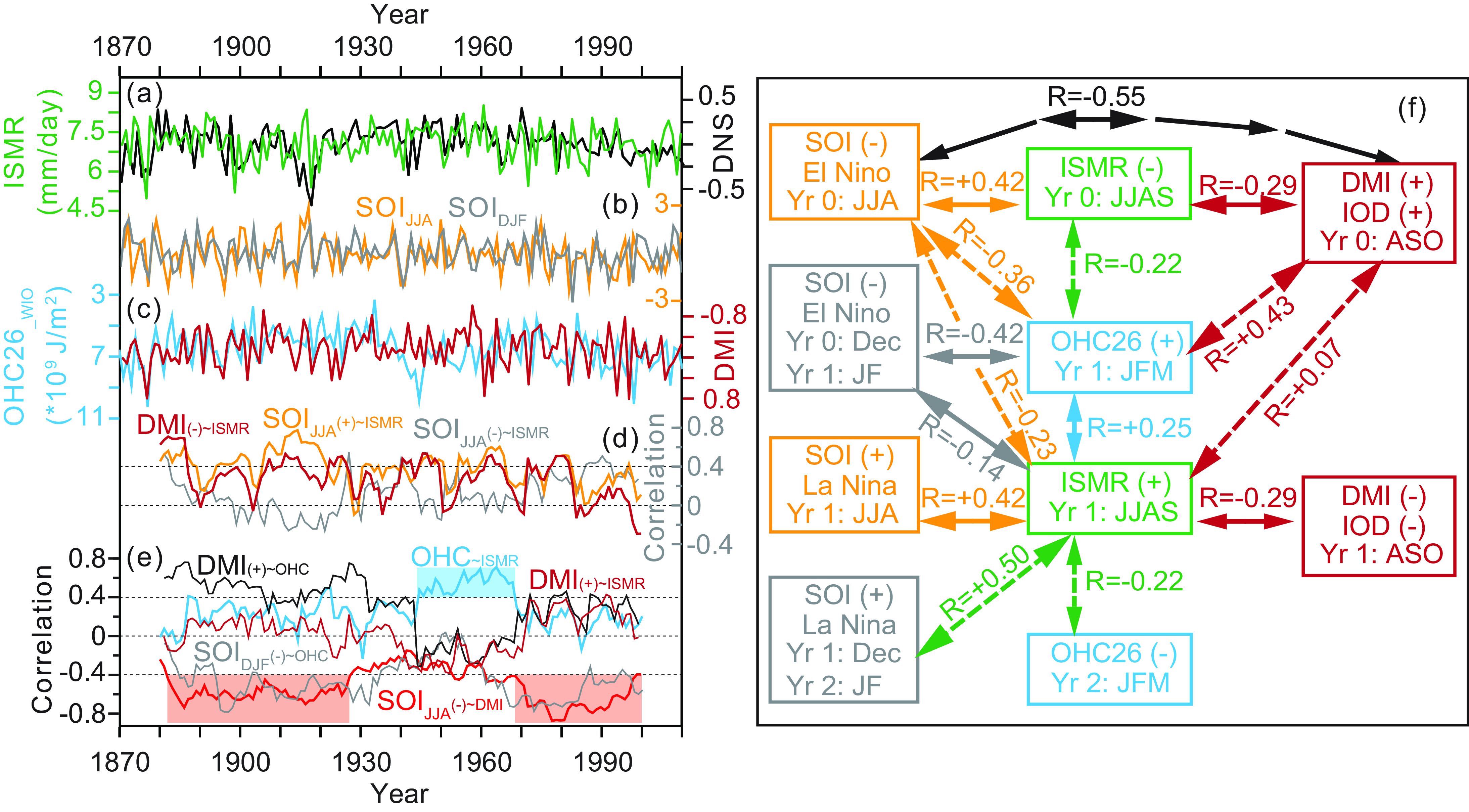
(a) Modern observed time series of ISM rainfall index (ISMR, green line) and ISM wind index (DNS, with linear trend removed, no units) from the year 1871 to 2010 AD. (b) Time series of SOI indexes during DJF and JJA (gray line for SOIDJF and orange line for SOIJJA, no units). (c) ASO DMI index (brown line, units: K) is compared with the OHC26_WIO time series (cyan line). (d) 20-year moving correlations for ISMR in Yr 1 with three indexes: DMI(-) in Yr 1 (multiplied by -1, brown line), SOIJJA(+) in Yr 1 (orange line), SOIJJA(-) in Yr 0 (gray line). (e) Moving correlations for OHC26_WIO in Yr 1 with three indexes: ISMR(+) in Yr 1 (cyan line), DMI(+) in Yr 0 (black line), SOIDJF(-) in Yr 1 (gray line), and for DMI (+) in Yr 0 with two indexes: ISMR(+) in Yr 1 (brown line), SOIJJA(-) in Yr 0 (red line). (f) Lead-lag correlations (R) between different time series. In (d), (e), and (f), those positive or negative signs in parentheses show the anomalous status of SOI, DMI, OHC26, and ISMR in the corresponding year.
(a) Regression coefficients of JJAS surface pressure (shaded) and 850 hPa horizontal winds (vector) against the normalized time series of ISM wind index (DNS). (b) is the same as (a) but with surface pressure replaced by JJAS rainfall (shaded). (c)–(d), (e)–(f), (g)–(h) are the same as (a)–(b) but for regression coefficients against the normalized time series of ISMR, of SOIJJA*(-1) in 1 year before, and of SOIJJA in the same year, respectively. Unless otherwise stated, grey dotted areas in all regression figures are significant at the 95% level with Student’s t-test, and small wind vectors (magnitude < 0.5 m/s) are not shown for clarity. For regression results, the character “(+)” or “(-)” means the normalized time series was multiplied by +1 or -1, and the character “lag0” or “lag1” means dependent variable lags independent variable (or the normalized time series) by 0 or 1 year.

Regression coefficients against modern observed time series (normalized). (a)–(b) are JAS and JFM OHC against the normalized DMI time series. (c) JFM OHC against ISMR time series. (d)–(e) JJAS surface pressure (shaded) and 850 hPa horizontal winds (vector) against DMI time series. (f) JJAS surface pressure (shaded) and 850 hPa horizontal winds (vector) against the OHC26_WIO time series. (g)–(i) are the same as (d)–(f) but with surface pressure replaced by JJAS rainfall (shaded). Black rectangular in (c) represents the region of WIO (5º S-15º N, 40º E-60º E) for calculating the OHC26_WIO time series. Note that the character of “lag0” in (c), (f) and (i) is relative to the year of higher ISMR or OHC26_WIO (Yr 1), and in other panels is relative to the year of higher DMI (Yr 0).

Composite differences of JJAS atmospheric variables between experiments CAM_control_TIOsst_JAS and CAM_control (a–b), between experiments CAM_control_TIOsst_JASP and CAM_control (c–d), between experiments CAM_control_TIOsst_JASN and CAM_control (e–f), and between experiments CAM_control_WIOsst_jfmP and CAM_control (g–h). The left panels are surface pressure (shaded) and 850 hPa winds (vectors, small winds (magnitude < 0.5 m/s) are not shown). The right panels are the same as the left panels but with surface pressure replaced by rainfall (shaded). Cyan contours and numbers in (b), (d), (f), and (h) show the spatial distributions of SST anomalies prescribed in each experiment. Characters of “∼DMI(+)” or “∼ISMR” means that these SST anomalies are regressed onto the DMI or ISMR maximum.

2.b. Paleoclimate simulations and proxies
As in Jian et al. (Reference Jian, Wang, Dang, Mohtadi, Rosenthal, Lea, Liu, Jin, Ye, Kuhnt and Wang2022), here we used the outputs from transient accelerated simulations of the Community Earth System Model 1.0.4 (CESM) (Shields et al. Reference Shields, Bailey, Danabasoglu, Jochum, Kiehl, Levis and Park2012), and of the water isotope (δ18O)-enabled air–sea coupled climate model from Goddard Institute for Space Studies of USA (GISS_ModelE2-R model) (Lewis et al. Reference Lewis, LeGrande, Schmidt and Kelley2014; Schmidt et al. Reference Schmidt, Kelley, Nazarenko, Ruedy, Russell, Aleinov, Bauer, Bauer, Bhat, Bleck, Canuto, Chen, Cheng, Clune, Del Genio, de Fainchtein, Faluvegi, Hansen, Healy, Kiang, Koch, Lacis, Legrande, Lerner, Lo, Matthews, Menon, Miller, Oinas, Oloso, Perlwitz, Puma, Putman, Rind, Romanou, Sato, Shindell, Sun, Syed, Tausnev, Tsigaridis, Unger, Voulgarakis, Yao and Zhang2014). The CESM was configured with T31_gx3v7 resolution (3.75º × 3.75º and vertical 27 levels for atmosphere, nominal 3º resolution, and vertical 60 levels for ocean). The GISS_ModelE2-R model has a horizontal resolution of 4º latitude ×5º longitude (both for the atmosphere and ocean), with 20 vertical layers in the atmosphere (up to 0.1 hPa) and 13 vertical layers in the Russell Ocean model (Russel et al. Reference Russell, Miller and Rind1995, Reference Russell, Miller, Rind, Ruedy, Schmidt and Sheth2000). Water isotope tracers (1H2 16O, “normal” water; 2H 1H 16O or HDO, reported as δD; and 1H2 18O, δ18O) are incorporated into the atmosphere, land surface, sea ice, and ocean (Schmidt et al. Reference Schmidt, Hoffmann, Shindell and Hu2005).
As a spin-up, these two models were run for 200 model years under fixed orbital parameters and greenhouse gases (GHG) of 300 ka BP, with all other boundary conditions (but neglecting ice sheet changes) set for their values in 1950 AD. Then, the models were integrated for 3000 model years with the transient orbital insolation forcing and GHG forcing of the last 300,000 years, in which orbital parameters and GHG were both advanced by 100 years at the end of each model year (Kutzbach et al. Reference Kutzbach, Liu, Liu and Chen2008). These two transient experiments are called CESM_ghg and GISS_ghg, respectively, and their outputs for the last 3000 model years are used in our analysis.
For experiment CESM_ghg, OHC above 26°C was first calculated using the same method as in modern observation, and then was linearly regressed onto the normalized ISMR index (Figs. 5a-c). Similar regression analysis was also applied to atmospheric variables (rainfall, horizontal winds and vertical p velocity) (Figs. 5d-f). Regionally averaged time series are calculated for annual mean SST over the Western Indian Ocean (10º S-10º N, 50º E-70º E, named as WIO_SST_CESM) and Eastern Indian Ocean (10º S-0º N, 85º E-105º E, called EIO_SST_CESM) to further calculate Dipole Mode Index (called DMI_CESM) (Figs. 6b–d, as in Wang et al. Reference Wang, Jian, Zhao, Chen and Xiao2015). Note that regional averaged time series of WIO, EIO, and DMI based on OHC26 are nearly the same as those of ocean mean temperature above 26°C and of SST, only time series of SST are shown in Fig. 6 for better comparison with paleo-proxy. ISMR_CESM and ISMR_GISS (Fig. 6e) represent regional averaged JJAS land rainfall from experiments CESM_ghg and GISS_ghg over the Indian subcontinent (10º N-30º N, 70º E-90º E), respectively. As referred to as δ18Osw_GISS (Fig. 6f), the annual mean δ18O of sea surface water (δ18Osw) from experiment GISS_ghg is regionally averaged over the Bay of Bengal (7º N-22º N, 80º E-100º E).
Regression coefficients against the normalized time series of ISMR_CESM from experiment CESM_ghg. (a)–(c) are JFM, JAS and annual mean OHC. (d) JJAS vertical p velocity (shaded) and meridional vertical circulation (vectors; meridional wind v and vertical p velocity) along the longitudes 85º E–120º E, (e) JJAS rainfall (shaded) and 850 hPa horizontal winds (vectors, small winds (magnitude < 2 m/s) are not shown). (f) JJAS vertical p velocity (shaded) and zonal-vertical circulation (vectors; zonal wind u and vertical p velocity) along the latitudes 5º S–5º N. White rectangular in (c) show the WIO and EIO regions for calculating DMI in simulations (Wang et al. Reference Wang, Jian, Zhao, Chen and Xiao2015). Yellow, white, and black filled dots in (c) show site locations of paleo-proxies (UK’ 37-SST, Mg/Ca-SST and δ18Osw). Character “ISMR(+)/Pmin” means that these anomalies are regressed onto the ISMR maximum (also the minimum of precession parameter).

Regional averaged time series of WIO_SST_CESM, EIO_SST_CESM, DMI_CESM, ISMR_CESM, ISMR_GISS, and δ18Osw_GISS from experiments CESM_ghg (black lines) and GISS_ghg (cyan and blue lines) are compared with multiple paleo-proxies: (a) Mg/Ca-SST of core WIND28K from the southwest Indian Ocean, (b) WIO stacked UK’ 37-SST, (c) EIO stacked UK’ 37-SST, (d) UK’ 37-SST based DMI, (f) the Bengal Bay δ18Osw_ivc. In (a)–(c), orange solid lines are residuals by subtracting 5-order polynomial-fitted trends (dashed lines) from the original time series (thin solid lines). The gray thick line in (a) is the precession parameter (Laskar et al. Reference Laskar, Robutel, Joutel, Gastineau, Correia, Correia and Levrard2004), and its minimas are marked by black vertical dashed lines.

Paleo-proxies used in Figure 6 are summarized in Table 1, including the planktonic foraminifera Globigerinoides ruber Mg/Ca-SST record of core WIND28K from the SWIO, the alkenone temperature (UK’ 37-SST) stacks of five cores from the WIO (GeoB3005, TY93929, MD85668, MD85674, VM19-193), and of three cores from the EIO (GeoB10038, SO139-74KL, MD2152). UK’ 37-SST based DMI was the difference between WIO and EIO. As a proxy of ISMR, ice-volume corrected δ18Osw was stacked by two cores from the Bay of Bengal (SO188-17286, U1446). All time series of paleo-proxy are interpolated to 1ka interval.
Paleo-proxy information used in this study

2.c. Equilibrium experiments with prescribed SST anomalies
Note that our transient simulations of CESM_ghg and GISS_ghg are both forced by atmospheric CO2 changes of 100 ppmv and seasonal solar insolation changes of about 80 W/m2. These two experiments enable us to investigate more acute changes of ISMR and its linkage with upper ocean thermal anomalies under extreme geological boundary conditions. Especially, the precessional insolation changes are much larger than those insolation changes at 41,000 years’ obliquity (about 30 W/m2) and the radiative forcing of CO2 doubling (3.7 W/m2). Thus, to compare with modern interannual variabilities without external forcing, here, we only focus on those paleoclimate changes at precessional band but neglect the effect of obliquity and CO2.
To isolate the role of IOD-like SST anomalies on ISMR, we also used outputs from equilibrium experiments of the CESM and its atmospheric component (the Community Atmospheric Model version 4, CAM4). Here, the CESM/CAM4 was run for 200/100 model years for each experiment, and the model outputs of the last 100/30 model years are analyzed. As detailed in Wang et al. (Reference Wang, Jian, Zhao, Xiao and Chen2016), the experiments CESM_control, CESM_Pmin, CAM_control, and CAM_Pmin are all set up with modern (1950_AD) greenhouse gas concentrations, topography, and land–sea distributions. The only difference between “control” and “Pmin” is precessional parameter (0.0169 vs −0.0169), and here “Pmin” actually means a precessional minimum of winter insolation and a maximum of summer insolation, respectively. Note that experiments CESM_Pmin and CESM_control will dynamically calculate SST (as a result of air–sea interactions) and their differences are treated as precession forced SST anomalies. To exclude the impact of these SST anomalies, experiments CAM_control and CAM_Pmin are prescribed with the same modern climatological monthly mean SST.
The equilibrium experiment CAM_Pmin_nptpsst is the same as CAM_Pmin but with modified SST over the North Pacific (20º N-50º N, 120º E-120º W) and tropical Pacific (20º S-20º N, 110º E-80º W). In these regions, precession forced climatological monthly mean SST anomalies are added to their modern values. Similarly, SST anomalies over TIO (20º S-25º N, 40º E-109º E) are added to CAM_Pmin in four different ways: (1) using values of 12 months (experiment CAM_Pmin_TIOsst), (2) only using values during JJA (experiment CAM_Pmin_TIOsst_JJA), (3) only using positive values during JJA (experiment CAM_Pmin_TIOsst_ JJAP), and (4) only using negative values during JJA (experiment CAM_Pmin_TIOsst_ JJAN).
As a comparison, by regressing onto the modern observed DMI index, monthly TIO SST anomalies during July–August–September (JAS) are added to experiment CAM_control in similar ways, resulting in another three equilibrium experiments: CAM_control_TIOsst_JAS, CAM_control_TIOsst_JASP, and CAM_control_TIOsst_JASN. Although summer NIO warming has been argued as a bridge from winter OHC to ISMR (Darshana et al. Reference Darshana, Chowdary, Gnanaseelan, Parekh and Srinivas2020), this mechanism should be better tested by the “pacemaker experiment” of fully coupled CESM model (Zhang et al. Reference Zhang, Han, Karnauskas, Meehl, Hu, Rosenbloom and Shinoda2019), which has beyond our ability. Thus, in experiment CAM_control_WIOsst_jfmP, we only use the JFM SST warming anomalies in WIO (5º S-15º N, 40º E-60º E) that are significantly correlated with modern observed ISMR index. It should be noted that these CAM4 experiments can only assess the direct impact of TIO SST on ISMR through atmospheric processes, but left the indirect influence through air–sea coupled feedbacks to future studies.
3. Results and discussion
3.a. Distinct modern dynamics associated with ISM wind and rainfall
Based on historical observations from the year 1871 to 2010 AD, we first compare the ISMR and the detrended DNS time series (Fig. 1a). Since the DNS is highly correlated with the South Asian (5º N-22.5º N, 35º E-97.5º E) averaged zonal wind at 850 hPa (R = +0.86, lag=0, p = 1.18*10-42), it is a reliable ISM wind intensity index. The correlation between DNS and ISMR is only +0.26 (lag = 0, p = 0.002), largely due to their similarity on multidecadal time scales. By comparing regression coefficients against the DNS index and the ISMR index, we found that they are associated with distinct changes of surface pressure, 850 hPa winds and rainfall anomalies (Figs. 2a-d).
For higher DNS, JJAS westerlies of ISM are enhanced from the Arabian Sea to the South China Sea (SCS) and can be explained by a stronger surface pressure gradient between the southwestern IO and Asian continent (Fig. 2a). Meanwhile, JJAS rainfall is increased over most regions of India, BOB, Indo-China Peninsula, and SCS, but is decreased over Bangladesh and the TIO (Fig. 2b). However, for higher ISMR, JJAS surface pressure anomalies are dominated by negative values over the WIO in contrast to those positive values over the Indo-China Peninsula and SCS (Fig. 2c), which induce larger magnitudes of anomalous easterlies from SCS to BOB (turning to south wind anomalies over India), and only left moderate magnitudes of anomalous westerlies over the southwestern Arabian Sea. Associated rainfall is decreased in the Indo-China Peninsula and SCS, but increased in the SWIO, equatorial Indonesia, and the South Asian region (5º N-30º N, 60º E-95º E) (Fig. 2d).
These results suggest that, although the stronger ISM westerlies due to land–sea pressure gradients can indeed result in higher ISMR at multi-decadal scales, the interannually increased ISM rainfall should be more related to anomalous easterlies due to surface high pressure and anticyclonic circulation from SCS to BOB. The latter linkage can be explained in the context of ENSO and IOD.
3.b. Interannual modulation of ENSO on ISMR relies on IOD
Consistent with previous studies (Annamalai et al. Reference Annamalai, Hamilton and Sperber2007; Wu RG et al. Reference Wu, Chen and Chen2012; Chakraborty, Reference Chakraborty2018), the SOIJJA and SOIDJF time series share much similarity (Fig. 1b) and their correlation with ISMR show clear seasonal inverse feature (Fig.1f). Before the spring of Year (Yr) 1, both SOIJJA (Yr 0) and SOIDJF (Yr 1) are weakly related to the increased ISMR in Yr 1 (R = −0.23 and −0.14, p = 0.01 and 0.11), but after spring, SOIJJA (Yr 1) and SOIDJF (Yr 2) are significantly correlated to ISMR in Yr 1 (R = +0.42 and +0.50, p = 3.13*10-7 and 5.54*10-10).
Regression coefficients against the minimum of SOIJJA (Yr 0, El Niño) and the maximum of SOIJJA (Yr 1, La Niña) (Fig. 2e–f and Fig. 2g–h) are both featured by increased ISMR during the summer of Yr 1, accompanying with anomalous surface high pressure, anticyclonic circulation from SCS to BOB. These SOIJJA associated anomalies are similar to those higher ISRM-associated changes (in Fig. 2c-d), and stand for two types of ENSO impact on ISMR (Wu RG et al. Reference Wu, Chen and Chen2012; Chowdary et al. Reference Chowdary, Chaudhari, Gnanaseelan, Parekh, Rao, Sreenivas, Pokhrel and Singh2014, Reference Chowdary, Parekh, Kakatkar, Gnanaseelan, Srinivas, Singh and Roxy2016; Chakraborty, Reference Chakraborty2018). One type is the lagged impact of decayed El Niño (from Yr0 JJA to Yr1 DJF) through the IPOC mechanism, the other is the simultaneous impact of developing La Niña through atmospheric circulation during the summer of Yr 1.
We noted that these two ENSO impacts show distinct responses in TIO that may be related to different phases of IOD. Since the SOIJJA and DMI time series have a significant correlation of −0.55 (p = 2.09*10-12), it means that a summer El Niño always appear with positive IOD event (or La Niña with negative IOD). This explains those differences in zonal surface pressure gradient in TIO: The west low-east high pressure pattern (Fig. 2e) reflects the persistent effect of positive IOD during the decayed El Niño phase, and the reversed gradient (Fig. 2g) may be influenced by negative IOD during the developing La Niña phase. How will these different phases of IOD impact on ISMR?
3.c. Positive IOD can greatly suppress ISMR in the same summer
Also consistent with previous studies (Saji et al. Reference Saji, Goswami, Vinayachandran and Yamagata1999; Gadgil et al. Reference Gadgil, Vinaychandran, Francis and Gadgil2004; Ihara et al. Reference Ihara, Kushnir, Cane and De la Peña2007), the correlation is +0.07 (lag = 1, p = 0.43) when ISMR lags DMI by 1 year (Fig. 1f), suggesting a poor lagged linkage from the DMI of Yr 0 to the ISMR of Yr 1. But this correlation becomes −0.29 (p = 0.0006) for lag = 0, indicating that ISMR will be significantly damped by positive IOD in the simultaneous summer. Similar to Li et al. (Reference Li, Lin and Cai2017), our regression coefficients against the maximum of DMI (Yr 0) are featured by anomalous surface westerlies from BOB to SCS, and reduced rainfall in most parts of India (Fig. 3d and 3g). This negative DMI–ISMR coherence in regression and correlation analysis seems to contradict with modern AGCM simulations, in which higher ISMR will be forced by positive IOD-like SST anomalies (Ashok et al. Reference Ashok, Guan, Saji and Yamagata2004, Reference Ashok, Behera, Rao, Weng and Yamagata2007). But recently it has been explained by the dominant influence of ENSO on ISMR overwhelming that of IOD (Li et al. Reference Li, Cai and Lin2016; Hrudya et al. Reference Hrudya, Varikoden and Vishnu2021). For example, during those time intervals of strong ENSO–IOD coherence, the ENSO–ISMR correlation is high, and the IOD–ISMR correlation is low (Ashok et al. Reference Ashok, Guan and Yamagata2001). So the decreased ISMR by El Niño may have much larger magnitude than the increased ISMR by positive IOD.
Our moving correlation shows that strong ENSO–IOD coherence mainly appears in two intervals of Yr 1883–1928 and of Yr 1969–1998 (red line in Fig. 1e). But these multidecadal (30-50 years) evolutions of ENSO–IOD coherence impact little on those of DMI–ISMR and SOIJJA–ISMR coherences, which only exhibit interdecadal (20 years) fluctuations. From Yr 1871–2010 AD, the negative correlation of DMI–ISMR (lag = 0) becomes stronger (close to or lower than −0.4) during those time intervals of larger SOIJJA–ISMR coherences (lag = 0) (brown and orange lines in Fig. 1d). It means that the ENSO–IOD coherence changes are hardly to explain the simultaneous negative relationship between ISMR and DMI.
Our modern sensitivity experiments of CAM4 suggest that, if forced by positive IOD-like SST anomalies during JAS, there will be only slightly increased summer rainfall over the northeastern BOB (Fig. 4b). More drastically is the decreased rainfall with anomalous surface high pressure and easterlies extending from the southwestern BOB to the Arabian Sea (Figs. 4a-4b). This anomalous meridional rainfall seesaw pattern is mainly contributed by the warmer WIO (Figs. 4c-4d), but only moderately cancelled by the cooler EIO (Figs. 4e-4f). Totally, ISMR is reduced by −0.15 mm/day over land, in which the warmer WIO and cooler EIO contribute to −0.27 mm/day and +0.12 mm/day, respectively.
Compared to previous studies that mainly emphasize the role of EIO cooling (Ashok et al. Reference Ashok, Guan and Yamagata2001, Reference Ashok, Guan, Saji and Yamagata2004; Krishnan et al. Reference Krishnan, Ramesh, Samala, Meyers, Slingo and Fennessy2006, Reference Krishnan, Sundaram, Sundaram, Swapna, Kumar, Kumar, Ayantika and Mujumdar2011), our CAM4 simulations illustrate the importance of WIO warming and provide another reasonable explanation for the damped ISMR by positive IOD in the simultaneous summer. Of course, the relative contributions of WIO and EIO to ISMR may be varied temporally and depend on particular IOD-like thermal gradient or the phase combination of IOD and ENSO, or the recent global warming background. For example, our summer WIO warming induces anomalous anticlockwise circulation over WIO of 10º S–20º N (Figs. 4a and 4c), which may weaken the climatological cross-equatorial low level jet stream and associated moisture transport into ISM regions. But this positive IOD induced feature mainly appears during those intervals of stronger ENSO–IOD coherence, and disappears in recent several decades with weaker ENSO–IOD coherence under global warming (Li et al. Reference Li, Cai and Lin2016; Hrudya et al. Reference Hrudya, Varikoden and Vishnu2021; Chakraborty and Singhai, Reference Chakraborty and Singhai2021).
3.d. Decayed IOD can also modulate upper OHC and ISMR
Moreover, the winter WIO warming during the decayed positive IOD or El Niño may also impact ISMR. Although the correlation between ISMR and JFM WIO OHC26 index (OHC26_WIO) from Yr 1871 to 2010 AD is only +0.25 (lag = 0, p = 0.0029), it is comparable to the simultaneous impact of DMI on ISMR (R = −0.29). For the JFM OHC26_WIO index, the largest correlation is 0.43 (p = 1.84*10-7) with DMI (+) of Yr 0, and is −0.42 (p = 2.17*10-7) with the SOIDJF of Yr 1 (Fig. 1f). Moving correlation further shows that, except for the time interval of Yr 1944-1968, its moving correlation with DMI (+) of Yr 0 is generally positive and comparable with its correlation with SOIDJF of Yr 1 (black and gray lines in Fig. 1e). And at multidecadal scales, both the DMI and SOIDJF show stronger coherence with OHC26_WIO during time intervals of strong ENSO–IOD coherence and vice versa. This probably indicates a significant role of WIO OHC on ISMR that depends on the interplay of ENSO and IOD.
But the OHC26_WIO only exhibits higher correlation (larger than +0.4) with ISMR during the interval of Yr 1944–1968 (cyan line and shaded in Fig. 1e), corresponding to a weakened ENSO-IOD coherence (red line in Fig. 1e). This interval is also accompanied with a sharply reduced correlation (from positive mean value of +0.5 to negative mean value of −0.13) between OHC26_WIO and DMI (+) of Yr 0 (black line in Fig. 1e). Although not significant, the correlation between DMI (+) of Yr 0 and ISMR also falls from positive to negative (brown line in Fig. 1e). This may suggest for a dominant role of IOD on the winter WIO OHC and associated ISMR, because there seems to be no similar sharp changes in the coherence between SOIDJF and OHC26_WIO (gray line in Fig. 1e).
Note that the simultaneous relation between DMI (or SOIJJA) and ISMR is still significant during this time interval (brown and orange lines in Fig. 1d), one possibility is that the concurrences of La Niña and negative IOD (both favoring increased ISMR) are relatively rare, as indicated by weakened SOIJJA–DMI coherence. More extremely, the damping effect of positive IOD on ISMR may largely cancel the increased ISMR during the summer of La Niña. In other words, the simultaneous effects of ENSO and IOD on ISMR will be greatly reduced during time interval of weakened SOIJJA–DMI coherence. This may result in a relative larger contribution of winter WIO OHC on ISMR and explain the significant coherence between them during Yr 1944-1968. But considering that most correlations among DMI, SOI, OHC, and ISMR during this interval are not significant, it is hard to resolve their true causal relationships. Here, we can only focus on the overall role of winter WIO OHC in bridging IOD and ISMR across the 20th century.
By regressing OHC26 onto the normalized timeseries of DMI (Figs. 3a-3b), we can see that positive IOD is accompanied by a zonal seesaw pattern of JAS OHC26 anomalies in the TIO, and those positive OHC26 anomalies in the WIO are still significant during JFM of next year. Interestingly, the higher ISMR-associated JFM OHC26 anomalies (Fig. 3c), JJAS surface pressure, 850hPa wind, and rainfall (Figs. 2c and 2d), all share many similarities with those of IOD-induced lagged air–sea anomalies (Figs. 3b, 3e and 3h). Note that similar features can also be found in those summer anomalies regressed onto OHC26_WIO (Figs. 3f and 3i), it, is reasonable to say that at interannual scales of the 20th century, historical positive IOD events can also greatly modulate the upper OHC in the TIO, and result in the increased OHC26_WIO during JFM of next year, then associated IPOC effect triggers anomalous high pressure and AAC over the SCS and BOB (Xie et al. Reference Xie, Kosaka, Du, Hu, Chowdary and Huang2016; Du et al. Reference Du, Chen, Xie, Zhang, Zhang and Cai2022), finally induce following JJAS ISM anomalies (surface easterlies and higher ISMR).
Using another modern sensitivity experiment of CAM4 (experiment CAM_control_WIOsst_jfmP), we can preliminarily illustrate the summer atmospheric response to the JFM SST warming anomalies in WIO. The rainfall increased over BOB and India south of 20º N but decreased over land regions north of 20º N (Fig. 4h), resulting a slightly reduced ISMR by −0.01 mm/day over land. Associated surface pressure and wind anomalies (Fig. 4g) also have smaller magnitudes and opposite signs relative to those summer SST induced changes (Figs. 4a and 4c). One reason is that the winter SST forcing (+0.1K to +0.2K in Figs. 4h) is smaller than the summer SST forcing of positive IOD (+0.4K to +0.6K in Figs. 4b). Another reason may be that those air–sea feedbacks following the winter WIO warming is also essential for the IPOC mechanism induced by positive IOD.
So far, we still cannot separate the delayed impacts of ENSO, IOD, and winter WIO warming on increased ISMR by regression analysis and CAM4 simulations. Although many studies highlighted the lagged impact of decayed El Niño on ISMR through IPOC (Mishra et al. Reference Mishra, Smoliak, Lettenmaier and Wallace2012; Darshana et al. Reference Darshana, Chowdary, Gnanaseelan, Parekh and Srinivas2020), here, we argue that when the coherence of El Niño and positive IOD (in Yr 0) is higher, the decayed IOD can also result in higher JFM WIO OHC in Yr 1, and may favor the following increased ISMR. In future studies, this IOD-induced lagged impact on ISMR should be not only further separated from the simultaneous impact of IOD, but also from those simultaneous and lagged anomalies induced by ENSO.
3.e. Precession forced paleo-IOD also dominates OHC and ISMR
Previous studies have shown that precessional insolation changes can induce significant tropical air–sea coupled responses assembling modern IOD mode (Abram et al. Reference Abram, Gagan, Liu, Hantoro, McCulloch and Suwargadi2007, Reference Abram, Hargreaves, Wright, Thirumalai, Ummenhofer and England2020; Brown et al. Reference Brown, Lynch and Marshall2009; Kwiatkowski et al. Reference Kwiatkowski, Prange, Varma, Steinke, Hebbeln and Mohtadi2015; Wang et al. Reference Wang, Jian, Zhao, Chen and Xiao2015; Mohtadi et al. Reference Mohtadi, Prange, Schefuß and Jennerjahn2017; Iwakiri & Watanabe, Reference Iwakiri and Watanabe2019; Windler et al. Reference Windler, Tierney and deMenocal2023). Associated zonal or meridional temperature/pressure gradients across the Indian Ocean may have greatly modulated hydroclimate changes in the African–Asian–Australian monsoon regions (Tierney et al. Reference Tierney, Oppo, LeGrande, Huang, Rosenthal and Linsley2012; Bolton et al. Reference Bolton, Chang, Clemens, Kodama, Ikehara, Medina-Elizalde, Paterson, Roberts, Rohling, Yamamoto and Zhao2013; deBoer et al. Reference de Boer, Tjallingii, Vélez, Rijsdijk, Vlug, Reichart, Prendergast, de Louw, Vincent Florens, Baider and Hooghiemstra2014; Weldeab et al. Reference Weldeab, Rühlemann, Ding, Khon, Schneider and Graya2022). But the role of upper OHC in bridging IOD and ISMR at orbital scales is still unclear.
Figure 5 illustrates those air–sea coupled paleoclimate changes associated with higher ISMR (mainly at the precession band) from experiment CESM_ghg. During JFM, negative OHC26 anomalies dominate large areas of the Indian Ocean (especially the northeastern and southwestern parts), largely as a result of decreased boreal winter insolation (Fig. 5a) (Wang et al. Reference Wang, Jian, Zhao, Chen and Xiao2015). While during JAS, OHC26 anomalies in Figure 5b are featured by a positive IOD-like zonal seesaw pattern (similar to modern observation, Fig. 3a), mainly induced by increased boreal summer insolation (Wang et al. Reference Wang, Jian, Zhao, Chen and Xiao2015). Annual mean OHC26 anomalies are generally dominated by those JAS OHC26 anomalies but also greatly reflect the contribution of JFM OHC26 anomalies (especially in the Indian Ocean south of 10º S) (Fig. 5c). The latter is also supported by the concurrence of precession parameter minima and the Mg/Ca-SST minimum of core WIND28K, reflecting decreased JFM insolation and mixed layer temperature (Fig. 6a).
In short, increased ISM rainfall at the precession band mainly corresponds to higher OHC26 in the equatorial WIO during boreal summer–autumn and also corresponds to lower OHC26 in the equatorial EIO during the whole year. Thus, the positive linkage between JFM OHC26_WIO and JJAS ISMR from modern interannual climate changes cannot be directly analoged to long-term paleoclimate changes, especially at the precession band with seasonal reversed insolation anomalies. It also means that the modern observed 1-year lagged response of ISMR to IOD through the bridging effect of JFM OHC26_WIO may be interrupted by external forcing (winter precessional insolation).
As shown in Figure 5e, higher ISMR is also accompanied by increased JJAS rainfall from the tropical Indian Ocean to equatorial Indonesia, but with reduced rainfall over the southeastern Indian Ocean, southern parts of the SCS and BOB. Note that these TIO rainfall anomalies between 15º S and 15º N are similar to modern IOD-related JJAS rainfall changes in CAM4 (Fig. 4b). Dose it means that the JJAS ISMR under precessional forcing may be also reduced by IOD-associated summer OHC anomalies in the tropical Indian Ocean?
Modern observation and simulation (Krishnan et al. Reference Krishnan, Ramesh, Samala, Meyers, Slingo and Fennessy2006, Reference Krishnan, Sundaram, Sundaram, Swapna, Kumar, Kumar, Ayantika and Mujumdar2011) suggest that due to intensified equatorial easterlies (during positive IOD), decreased upper OHC prevails with shallower mixed layer and local atmospheric subsidences in the equatorial EIO from June to August, which further induces remote upward motions over India through meridional vertical atmospheric circulation anomalies, and induce increased ISMR through stronger cross-equatorial monsoon flow and moisture export from the southeast Indian Ocean (Behera et al. Reference Behera, Krishnan and Yamagata1999; Ashok et al. Reference Ashok, Guan, Saji and Yamagata2004). Paleoclimate proxies and simulation also show that upper ocean thermal structure changes in the EIO (and associated zonal/meridional thermal gradients) during boreal summer–autumn can significantly modulate ISM, generally with cooler EIO corresponding to stronger ISM westerlies or increased monsoon rainfall (Bolton et al. Reference Bolton, Chang, Clemens, Kodama, Ikehara, Medina-Elizalde, Paterson, Roberts, Rohling, Yamamoto and Zhao2013; Weldeab et al. Reference Weldeab, Rühlemann, Ding, Khon, Schneider and Graya2022). This represents a direct atmospheric linkage from the EIO to ISM during boreal summer.
Considering that the ice sheet was fixed as modern values and the ice-albedo feedback was muted in our transient simulation, the modeled glacial–interglacial climatic changes may be underestimated and hinder the direct comparison with proxy data. In Figures 6a–6c, we choose to remove the long-term trend (dashed lines) from SST proxies using 3-order polynomial fitting method and ignore those proxy-model discrepancies in magnitudes of short term changes. After detrending, those UK’ 37-SST residuals in WIO and EIO (orange lines) show many similarities with our simulated SST (black lines) and only just lack some precessional cycles (Figs. 6b-6c). Consistent with our simulated DMI, UK’ 37-SST based DMI is also dominated by precessional cycles except for the time interval of 120∼200 ka (Fig. 6d). Moreover, these precessional cycles of two DMI indexes seem to be more contributed by EIO changes that are out of phase with ISMR (Figs. 6c–6e). Thus, it seems that our transient simulations and paleo-proxies all support the notion of EIO-dominated IOD modulation on ISMR at the precession band.
3.f. Relative role of IOD, ENSO, and land–sea thermal contrast on ISMR at the precession band
Our simulated paleo-IOD also prevails with anomalous equatorial easterlies from the central Pacific Ocean to the WIO (Figs. 5e-5f), indicating that the climatological summer Walker circulation is enhanced over the western to central Pacific but weakened over TIO (Wang et al. Reference Wang, Jian, Zhao, Chen and Xiao2015, Reference Wang, Jian, Zhao, Xu, Dang, Liu, Xiao and Chen2019; Wang et al. Reference Wang, Jian, Lückge, Wang, Dang and Mohtadi2018). This is in contrast to the modern observed positive IOD and El Niño combination and reflects the independent TIO response under external forcing. To explain the coupling between the two anomalous zonal-vertical circulations, we identified a meridional wave-like pattern of those rainfall anomalies (negative-positive-negative-positive) from the southeast TIO to ISM region (Fig. 5e). This meridional pattern represents three local anomalous meridional vertical atmospheric circulations (with descent-ascent-descent-ascent from south to north) (Fig. 5d), probably excited by the colder SST and atmospheric subsidence in the EIO, or by the summer oceanic warming and atmospheric upward motions in the WIO.
Although we highlight the modulation of IOD on ISMR, the precession-forced La Niña-like conditions in the western-central Pacific Ocean may also contribute to the higher ISMR. More importantly, orbital changes of ISMR (Figs. 5e and 6e) have been largely attributed to land–sea thermal difference at the precession band (Wang et al. Reference Wang, Jian, Zhao, Xiao and Chen2016). Here, we further assess the relative contribution of land–sea contrast, ENSO and IOD on ISMR based on sensitivity experiments of CAM4. As a start, the influence of land–sea thermal gradient under precessional forcing can be illustrated by those JJAS differences between experiments CAM_Pmin and CAM_control (Figs. 7a-7b), which are featured by anomalous surface high pressure and AAC over the North Indian Ocean, and by reduced rainfall in regions of 5º S–20º S and of 5º N–20º N, but with increased rainfall in regions of 5º S–5º N and north of 20º N. Then composite differences between experiments CAM_Pmin_nptpsst and CAM_Pmin show that the Pacific SST anomalies can induce anomalous surface low pressure and westerlies over South Asia and increased rainfall over India, BOB, and SCS regions (Figs. 7c-7d). It means that the precessional forced summer “central Pacific type” La Niña-like pattern (Wang et al. Reference Wang, Jian, Zhao, Xu, Dang, Liu, Xiao and Chen2019) can produce stronger ISM westerlies and higher ISMR.
Composite differences of JJAS atmospheric variables between experiments CAM_Pmin and CAM_control (a–b), between experiments CAM_Pmin_nptpsst and CAM_Pmin (c–d), and between experiments CAM_Pmin_TIOsst and CAM_Pmin (e–f). The left panels are surface pressure (shaded) and 850 hPa horizontal winds (vectors, small winds (magnitude < 0.5 m/s) are not shown). The right panels are the same as the left panels but with surface pressure replaced by rainfall (shaded). Characters in parentheses show the forcing factor for composite differences in each panel.

As shown by composite differences between experiments CAM_Pmin_TIOsst and CAM_Pmin, TIO SST anomalies during all seasons induce anomalous surface high pressure and more drastically reduced rainfall in the northern Arabian Sea and India (15º N-25º N), and in BOB and SCS regions (10º N-25º N) (Figs. 7e–7f). Meanwhile, significant anomalous low pressure and increased rainfall occupy the WIO and the EIO of 0º N–10º N. Additional CAM4 experiments (CAM_Pmin_TIOsst_JJA, CAM_Pmin_TIOsst_JJAP, and CAM_Pmin_TIOsst_JJAN) prove that, the meridional wave-like pattern of summer rainfall from the southeast TIO to ISM region is mainly contributed by summer WIO SST anomalies (as shown by Figs. 8b and 8d). And they are accompanied by anomalous surface easterlies extending from the southwestern BOB to the Arabian peninsula, and by anomalous cross-equatorial northerlies over WIO of 10º S–20º N (Figs. 8a and 8c). Although these precessional forced anomalies are similar to those induced by modern positive IOD (Figs. 4a–4b), the EIO wave-like rainfall pattern seems have larger meridional extension (Fig. 8b relative to Fig. 4b). This may indicate larger contributions from those SST warming anomalies in WIO and the EIO of 0º N–10º N, but can also be attributed to the smaller magnitudes of SST cooling in the southeast TIO (−0.1 K–−0.2 K, cyan contours in Fig. 8b) relative to modern situations (−0.2 K–−0.6 K in Fig. 4b).
Similar to Figure 7, but for composite differences between experiments CAM_Pmin_TIOsst_JJA and CAM_Pmin (a–b), between experiments CAM_Pmin_TIOsst_ JJAP and CAM_Pmin (c–d), and between experiments CAM_Pmin_TIOsst_ JJAN and CAM_Pmin (e–f). Cyan contours in (b), (d), (f), and (h) show the spatial distributions of SST anomalies prescribed in each experiment.

Note that the Pacific SST tends to increase the ISM rainfall everywhere, but the effect of TIO SST and land–sea contrast are spatially inhomogeneous over the Indian subcontinent (wetter north and drier south). Totally, the ISMR is increased by +0.69 mm/day for the land–sea contrast effect and by +0.52 mm/day for the Pacific SST, but is decreased by −0.48 mm/day for the TIO SST effect. For this damping effect of TIO SST, the summer IOD-like SST anomalies only contribute −0.16 mm/day because of the mutually offsetting by WIO warming (−0.44 mm/day) and EIO cooling (+0.28 mm/day). Thus, large parts (−0.32 mm/day) of the TIO damping effect actually should be attributed to SST anomalies of autumn, winter, and spring. Moreover, if TIO SST anomalies were added to experiment CAM_Pmin_nptpsst (rather than experiment CAM_Pmin), although associated anomalous rainfall pattern is similar, the TIO damping effect will become −0.79 mm/day and the ISMR will be only increased by +0.42 mm/day relative to experiment CAM_control. It means there exist significant nonlinear interactions in atmosphere when combined SST forcing from different regions.
Finally, in our equilibrium CESM simulations (experiments CESM_Pmin and CESM_control), the ISMR is increased by +1.58 mm/day, close to the difference of +1.71 mm/day between 10ka and 0ka in the experiment CESM_ghg (Fig. 6e). This includes not only those positive contributions from land–sea contrast and paleo-ENSO (+1.2mm/day), but also the damping effect of TIO SST in different seasons (−0.48 or −0.79 mm/day, including but not limited to paleo-IOD). Clearly, there is a large gap in the magnitude of ISMR changes between CESM and CAM4. In other words, the real contribution of positive paleo-IOD to higher ISMR requires further studies by considering the role of air–sea feedbacks.
4. Conclusion and final remarks
In this study, we comprise modern observation, paleoclimate simulation and proxy reconstruction, trying to investigate the modulation of IOD and associated TIO OHC on the Indian summer monsoon rainfall from interannual to orbital time scales.
Based on historical observations from the year 1871 to 2010 AD, we illustrated that those air–sea coupled dynamics associated with ISM rainfall are entirely different from those of ISM wind at interannual time scales. While stronger ISM wind (westerlies) can indeed result in higher ISMR at the expense of a drier TIO, higher ISMR is generally associated with surface high pressure, easterly wind and reduced rainfall anomalies from SCS to BOB. These higher ISMR-associated anomalies can be firstly attributed to two types of ENSO influence, (1) the simultaneous atmospheric circulation changes of developing La Niña in Yr 1 and (2) the lagged air–sea coupled IPOC effect of decayed El Niño since Yr 0, probably bridged by the increased WIO OHC above 26°C during boreal winter–spring.
We argue that this higher ISMR-associated winter OHC anomaly can also be attributed to positive IOD conditions one year before, and this linkage is enhanced with a stronger ENSO-IOD coherence at multidecadal time scales. But the positive correlation between ISMR and winter WIO OHC is insignificant during those time intervals of stronger ENSO–IOD coherence (Yr 1883–1928 and 1969–1998). Our sensitivity experiments of CAM4 further prove that, the winter WIO SST warming anomalies only induce slightly increased ISM rainfall south of 20º N and decreased rainfall north of 20º N, while those summer positive IOD-like SST anomalies result in drastically decreased rainfall from the southwestern BOB to the northern Arabian Sea. Totally, the ISMR is changed by +0.01 and -0.15mm/day due to these two kinds of SST anomalies. It means that the impact of winter WIO OHC on ISMR through IPOC mechanism is only secondary, probably overwhelmed by the simultaneous impacts of El Niño and positive IOD.
By comparing paleoclimate simulation and paleo-proxies, we found that modern interannual positive linkage between ISMR and winter WIO OHC was cut off by seasonal reversed insolation anomalies at the precessional band. But our CAM4 experiments also prove the precessional forced ISMR can be simultaneously damped by positive IOD-like OHC anomalies in the summer TIO. Similar to modern situations, we identified a meridional wave-like pattern of summer rainfall anomalies from the southeast TIO to ISM region, and the drastically decreased rainfall in the southern ISM region dominates the total ISMR changes. This damping effect is mainly contributed by the warmer western TIO that triggers anomalous easterlies along the southern flank of surface high pressure anomalies from BOB to Arabian Peninsula. And the cooler southeastern TIO will only moderately increase rainfall in the southern ISM region.
Finally, our transient simulation results are generally consistent with paleo-temperature proxies from the tropical Indian Ocean, and the simulated δ18Osw_GISS in the Bay of Bengal from experiment GISS_ghg are also similar to ISMR and negative δ18O peaks are nearly in phase with high ISM rainfall (Figs. 6e–6f), confirming the dominant role of ISMR on the freshwater supplement to the Bay of Bengal (Clemens et al. Reference Clemens, Yamamoto, Thirumalai, Giosan, Richey, Nilsson-Kerr, Rosenthal, Anand and McGrath2021; Tabor et al. Reference Tabor, Otto-Bliesner, Brady, Nusbaumer, Zhu, Erb, Wong, Li and Noone2018). Our simulated δ18Osw_GISS shows large discrepancies relative to the proxy-reconstructed δ18Osw_ivc (Fig. 6f), probably due to the coarse resolution and model limitation of our GISS_ModelE2-R model, or due to the errors of temperature correction and seasonal biases of δ18Osw_ivc proxy, which all require for more future studies.
Acknowledgements
This work was supported by the National Natural Science Foundation of China (Y.W., grant number 41976047), (X.W., grant number 42106060), (S.Z., grant number 42376053), (H.D., grant number 42176053, 42222603), and (Z.J., grant numbers 42188102, 91958208). Y.W. is also sponsored by the National Key Research and Development Program of China (grant number: 2023YFF0803904) and by the Shanghai Pilot Program for Basic Research. Y.W. acknowledges the Shanghai Supercomputer Center and the Beijing Super Cloud Computing Center (BSCC) for providing HPC resources that have contributed to the research results reported within this paper.
Competing interests
The authors declare none.


 Open access