


Impact statement
Whilst the installed capacity of wind power is increasing rapidly worldwide, there is no consensus on how the design and operation of large wind farms should be optimised. The difficulty lies in wind farm power losses being dependent on complex flow phenomena across a wide range of scales. The significance of this theoretical work is that it describes the interaction of all aerodynamic power losses in a wind farm using a closed set of physics-based algebraic equations, considering the first-order effects of turbine design, layout, operation and atmospheric conditions. This allows us to quickly estimate the relationship between the farm power and the farm induction factor, the latter of which has implications for wind farm wakes and their impacts on the surroundings. Therefore, this work provides a theoretical basis that can improve the process of wind farm design, site selection and environmental impact assessment in the future.
1. Introduction
Wind farm aerodynamics is a relatively new and rapidly growing subject in applied fluid mechanics. In contrast to the fundamentals of rotor aerodynamics having been well explained (by the classical blade-element momentum theory of Glauert (Reference Glauert and Durand1935), for example) and considered in the design of modern wind turbines, our understanding of wind farm aerodynamics is still immature, leaving some basic questions unresolved for today’s wind power industry. The challenge in wind farm aerodynamics stems from its multiscale nature (Veers et al. Reference Veers2019; Porté-Agel et al. Reference Porté-Agel, Bastankhah and Shamsoddin2020) and the large number of parameters involved, ranging from regional weather conditions to the layout, design and operating conditions of individual turbines in the farm, resulting in a high-dimensional optimisation problem to consider. To provide a holistic view of wind farm performance, i.e. a physics-based prediction of how different types of power losses in a wind farm would change across the entire parameter space, it is necessary to develop a comprehensive theoretical model of wind farm aerodynamics.
A series of recent studies regarding ‘two-scale momentum theory’ (Nishino Reference Nishino2016; Nishino & Hunter Reference Nishino and Hunter2018; Nishino & Dunstan Reference Nishino and Dunstan2020; Kirby et al. Reference Kirby, Nishino and Dunstan2022, Reference Kirby, Dunstan and Nishino2023, Reference Kirby, Nishino, Lanzilao, Dunstan and Meyers2025) contributes to this goal. The first theoretical model proposed by Nishino (Reference Nishino2016) was similar to the classical ‘top-down’ wind farm models (Calaf et al. Reference Calaf, Meneveau and Meyers2010; Emeis & Frandsen Reference Emeis and Frandsen1993; Frandsen Reference Frandsen1992) with a key difference being that it introduced the concept of ‘farm-layer-average’ wind speed to avoid considering the vertical profile of the atmospheric boundary layer (ABL) explicitly. The advantage of not explicitly considering the ABL profile was not obvious at the time, as these early models were for infinitely large wind farms and thus their applications to real wind farms were limited. Around the same time, Stevens et al. (Reference Stevens, Gayme and Meneveau2016) derived a coupled wake boundary layer (CWBL) model by coupling a traditional turbine-wake model (Jensen Reference Jensen1983; Katić et al. Reference Katić, Højstrup and Jensen1986) with the top-down model of Calaf et al. (Reference Calaf, Meneveau and Meyers2010), showing good agreement with large-eddy simulation (LES) studies of a finite-size wind farm; however, difficulties in comparing with real wind farm data remained, as some of the model input parameters were uncertain from field measurements. The advantage of focusing on the farm-layer-average wind speed became clearer when the concept of ‘momentum availability’ was introduced by Nishino and Dunstan (Reference Nishino and Dunstan2020), generalising the two-scale theory to consider finite wind farms of different sizes, and subsequently its analytical ‘sub-models’ by Kirby et al. (Reference Kirby, Dunstan and Nishino2023) (n.b. ‘sub-models’ means ‘constituent models’ of a wind farm model based on the two-scale theory). These analytical sub-models require only limited information of the ABL (and the wind farm size) to predict the momentum availability, which in turn allows us to predict the farm-average wind speed for a given wind farm analytically. As will be discussed later in this paper, the two-scale momentum theory provides a basic framework for the modelling of wind farm aerodynamics, upon which different types of sub-models (either analytical or numerical, with different levels of complexity depending on the type of information available for the model input) can be developed and employed to predict the performance of a given wind farm in a given environment.
Another key feature of the two-scale momentum theory is that it provides a different view of power loss mechanisms for large wind farms (Kirby et al. Reference Kirby, Nishino and Dunstan2022, Reference Kirby, Nishino, Lanzilao, Dunstan and Meyers2025) from a traditional view based on the superposition of turbine-wake models (Jensen Reference Jensen1983; Katić et al. Reference Katić, Højstrup and Jensen1986; Bastankhah & Porté-Agel Reference Bastankhah and Porté-Agel2014; Nygaard et al. Reference Nygaard, Steen, Poulsen and Pedersen2020). In short, the traditional view is that the (aerodynamic) power loss in a wind farm is due to individual turbine wakes reducing the inflow speed for downstream turbines. This traditional view has been expanded over the last decade as the effect of ‘wind farm blockage’ (Allaerts & Meyers Reference Allaerts and Meyers2017; Bleeg et al. Reference Bleeg, Purcell, Ruisi and Traiger2018; Wu & Porté-Agel Reference Wu and Porté-Agel2017) has been widely recognised and some analytical farm-blockage models (Branlard & Meyer Forsting Reference Branlard and Meyer Forsting2020; Nygaard et al. Reference Nygaard, Steen, Poulsen and Pedersen2020; Segalini Reference Segalini2021) have been developed. However, a common view in today’s wind industry is still that the power loss in a single wind farm is mostly due to turbine–wake interactions since the reduction of inflow speed for ‘front-row’ turbines is usually (much) smaller than that for downstream turbines, i.e. only the wind reduction ‘upstream’ of a whole farm is attributed to the farm-blockage effect. In contrast to this, the view provided by the two-scale theory is that the power loss in a large wind farm is primarily due to farm-scale flow interactions between the atmosphere and the farm as a whole, causing a reduction of ‘farm-average’ wind speed (similarly to the concept of top-down models for infinitely large wind farms) as well as ‘farm-upstream’ wind speed, while individual turbine–wake interactions within the farm may cause some additional power losses depending on the turbine layout. Kirby et al. (Reference Kirby, Nishino, Lanzilao, Dunstan and Meyers2025) have recently reported a detailed analysis of finite-size wind farm LES results to show that the ‘wind extractability’ for a whole farm (i.e. rate of change of momentum availability for the whole farm with respect to the farm-average wind speed) is dependent on the farm size, but insensitive to the turbine layout, suggesting that the view provided by the two-scale theory is more plausible when the farm is large enough. It is still an open question how large the farm needs to be for this view to be valid, since the LES data for finite-size wind farms are limited, but the smallest wind farm length considered by Kirby et al. (Reference Kirby, Nishino, Lanzilao, Dunstan and Meyers2025) (in a representative offshore ABL of 500 m height) was approximately 7 km. Hence, as a rule of thumb, we shall use the term ‘large wind farm’ in the present paper when the farm length is at least an order of magnitude larger than the ABL height. We focus mainly on offshore wind farms in this paper, although the theory is, in principle, applicable to flat onshore wind farms as well.
The concept of farm-average wind reduction or ‘farm induction’ may play a key role in predicting not only the power of a single farm, but also the strength of ‘farm wake’ and thus the power of another farm located downstream (Lundquist et al. Reference Lundquist, DuVivier, Kaffine and Tomaszewski2019; Meyers et al. Reference Meyers, Bottasso, Dykes, Fleming, Gebraad, Giebel, Göçmen and van Wingerden2022; Stieren & Stevens Reference Stieren and Stevens2022). The two-scale theory and its analytical sub-models allow very fast predictions of farm induction; however, the main interest of previous theoretical studies (Kirby et al. Reference Kirby, Dunstan and Nishino2023; Nishino & Dunstan Reference Nishino and Dunstan2020) was to predict an upper limit to the power of a single farm and thus the studies were mostly limited to ‘ideal’ wind farm scenarios, considering aerodynamically ideal turbines (or actuator discs) in a hypothetical array where the inflow speed for each turbine was assumed to agree with the farm-average wind speed. In this study, we extend the two-scale theory to account for the thrust and power characteristics of real turbine rotors, as well as the effects of arbitrary turbine layout and wind direction. We will also present a simple iterative method for calculating the optimal farm induction factor that maximises the power of a given wind farm. In addition to presenting these new results, another purpose of the present paper is to provide a concise and up-to-date description of the background theory for future reference.
2. Background theory
We summarise the existing two-scale momentum theory and its analytical sub-models in this section, before describing the new additions in the next section. A schematic of the flow configuration and a list of input parameters for the present theoretical model (including the new additions) are shown in Figure 1.
Schematic of flow configuration and a list of input parameters for the extended theoretical model. Note that, to calculate the non-dimensional farm power, only the non-dimensional parameters (
 $\lambda /C_{f0}, h_0/LC_{f0},C_T^{\textrm { Rat}},C_P^{\textrm {Rat}},\chi _T$
and
$\lambda /C_{f0}, h_0/LC_{f0},C_T^{\textrm { Rat}},C_P^{\textrm {Rat}},\chi _T$
and
 $\chi _P$
) are required as input. In addition to these parameters, one additional input (typically
$\chi _P$
) are required as input. In addition to these parameters, one additional input (typically
 $C_T$
to obtain
$C_T$
to obtain
 $\beta$
, or vice versa) is required to solve the problem.
$\beta$
, or vice versa) is required to solve the problem.

2.1. Two-scale momentum theory
The core idea of the theory proposed by Nishino and Dunstan (Reference Nishino and Dunstan2020) (hereafter referred to as ND20) is that a large wind farm is considered as a single power generation device (or an actuator volume) which imposes ‘farm-scale’ resistance to the ABL flow and thus reduces ‘farm-average’ wind speed as it generates power. Hence, the most important parameter describing the overall state of the farm (at a given time, i.e. averaged over a short period of time, typically 10 minutes) is its wind-speed reduction factor defined as
 \begin{equation} \beta \equiv \frac {U_F}{U_{F0}} , \end{equation}
where
 $U_F$
and
$U_F$
and
 $U_{F0}$
are the farm-average wind speeds for the cases with and without the farm present, respectively, and the farm induction factor can also be defined as
$U_{F0}$
are the farm-average wind speeds for the cases with and without the farm present, respectively, and the farm induction factor can also be defined as
 $b\equiv (1-\beta )\equiv (U_{F0}-U_F)/U_{F0}$
. This is analogous to the classical actuator disc theory for a single turbine, where the state of airflow through the turbine is described using the axial induction factor defined as
$b\equiv (1-\beta )\equiv (U_{F0}-U_F)/U_{F0}$
. This is analogous to the classical actuator disc theory for a single turbine, where the state of airflow through the turbine is described using the axial induction factor defined as
 $a\equiv (U_{T0}-U_T)/U_{T0}$
, where
$a\equiv (U_{T0}-U_T)/U_{T0}$
, where
 $U_T$
and
$U_T$
and
 $U_{T0}$
are ‘turbine-average’ wind speeds for the cases with and without the turbine present, respectively. In reality, neither the flow through a turbine nor the flow through a farm is perfectly uniform. Nonetheless, the average wind speed reduction is the key factor in each problem as it captures the first-order effect of power generation on the undisturbed wind, which in turn determines the amount of wind power extractable by a device (turbine or farm) and the strength of its wake.
$U_{T0}$
are ‘turbine-average’ wind speeds for the cases with and without the turbine present, respectively. In reality, neither the flow through a turbine nor the flow through a farm is perfectly uniform. Nonetheless, the average wind speed reduction is the key factor in each problem as it captures the first-order effect of power generation on the undisturbed wind, which in turn determines the amount of wind power extractable by a device (turbine or farm) and the strength of its wake.
A key question in the two-scale momentum theory is how to define the nominal ‘farm-layer height’ across which the farm-average wind speeds
 $U_F$
and
$U_F$
and
 $U_{F0}$
are calculated. Unlike the actuator disc theory for a single turbine, where the rotor swept area
$U_{F0}$
are calculated. Unlike the actuator disc theory for a single turbine, where the rotor swept area
 $A$
is an obvious choice for the area across which the turbine-average wind speeds
$A$
is an obvious choice for the area across which the turbine-average wind speeds
 $U_T$
and
$U_T$
and
 $U_{T0}$
are calculated, there is no obvious choice for the farm-layer height in the two-scale theory. Essentially, different choices of the farm-layer height lead to different values of ‘reference’ wind speed
$U_{T0}$
are calculated, there is no obvious choice for the farm-layer height in the two-scale theory. Essentially, different choices of the farm-layer height lead to different values of ‘reference’ wind speed
 $U_{F0}$
for non-dimensionalisation. The original definition of the farm-layer height
$U_{F0}$
for non-dimensionalisation. The original definition of the farm-layer height
 $H_F$
adopted by ND20 is such that it gives
$H_F$
adopted by ND20 is such that it gives
 $U_{F0}=U_{T0}$
. This definition leads to a concise description of power loss mechanisms, as shown later, although the vertical profile of the undisturbed wind speed,
$U_{F0}=U_{T0}$
. This definition leads to a concise description of power loss mechanisms, as shown later, although the vertical profile of the undisturbed wind speed,
 $U_0(z)$
, is required to calculate
$U_0(z)$
, is required to calculate
 $H_F$
. When the vertical profile of the ABL is unknown, the exact value of
$H_F$
. When the vertical profile of the ABL is unknown, the exact value of
 $H_F$
(that gives
$H_F$
(that gives
 $U_{F0}=U_{T0}$
) cannot be calculated; however, the concept of farm-layer average (across an unknown height
$U_{F0}=U_{T0}$
) cannot be calculated; however, the concept of farm-layer average (across an unknown height
 $H_F$
) remains useful. As described later in § 2.2, Kirby et al. (Reference Kirby, Dunstan and Nishino2023) have derived an analytical sub-model of the two-scale theory to predict the farm-layer-average wind reduction factor
$H_F$
) remains useful. As described later in § 2.2, Kirby et al. (Reference Kirby, Dunstan and Nishino2023) have derived an analytical sub-model of the two-scale theory to predict the farm-layer-average wind reduction factor
 $\beta$
without using
$\beta$
without using
 $H_F$
as input. It is also worth noting that
$H_F$
as input. It is also worth noting that
 $H_F \approx 2.5H_{hub}$
(where
$H_F \approx 2.5H_{hub}$
(where
 $H_{hub}$
is the hub height of turbine rotors) was found to be a good approximation of the exact
$H_{hub}$
is the hub height of turbine rotors) was found to be a good approximation of the exact
 $H_F$
for a range of turbine designs and neutral ABL profiles (Kirby et al. Reference Kirby, Nishino and Dunstan2022).
$H_F$
for a range of turbine designs and neutral ABL profiles (Kirby et al. Reference Kirby, Nishino and Dunstan2022).
The essence of the two-scale momentum theory lies in the expression of the non-dimensional farm momentum (NDFM) equation, derived from the law of conservation of linear momentum for the cases with and without the farm present (ND20, see also Kirby et al. Reference Kirby, Nishino and Dunstan2022). The final form of the NDFM equation, from which the wind reduction factor
 $\beta$
can be calculated, is
$\beta$
can be calculated, is
 \begin{equation} C_T^* \frac {\lambda }{C_{f0}} \beta ^2 + \beta ^\gamma = M, \end{equation}
where the first and second terms on the left-hand side are the total turbine drag (
 $\Sigma _{i=1}^N T_i$
, where
$\Sigma _{i=1}^N T_i$
, where
 $N$
is the number of turbines in the farm) and the surface friction drag (
$N$
is the number of turbines in the farm) and the surface friction drag (
 $\tau _w S_F$
, where
$\tau _w S_F$
, where
 $S_F$
is the horizontal area of the farm) that are both normalised by the ‘undisturbed’ surface friction drag (
$S_F$
is the horizontal area of the farm) that are both normalised by the ‘undisturbed’ surface friction drag (
 $\tau _{w0}S_F$
). Note that
$\tau _{w0}S_F$
). Note that
 $C_T^*\equiv \Sigma _{i=1}^N T_i/\frac {1}{2}\rho U_F^2NA$
is the ‘internal’ thrust coefficient (defined using
$C_T^*\equiv \Sigma _{i=1}^N T_i/\frac {1}{2}\rho U_F^2NA$
is the ‘internal’ thrust coefficient (defined using
 $U_F$
instead of
$U_F$
instead of
 $U_{F0}$
),
$U_{F0}$
),
 $\lambda \equiv NA/S_F$
is the array density,
$\lambda \equiv NA/S_F$
is the array density,
 $C_{f0}\equiv \tau _{w0}/\frac {1}{2}\rho U_{F0}^2$
is the surface friction coefficient (defined using
$C_{f0}\equiv \tau _{w0}/\frac {1}{2}\rho U_{F0}^2$
is the surface friction coefficient (defined using
 $U_{F0}$
instead of the wind speed at 10 m height) and
$U_{F0}$
instead of the wind speed at 10 m height) and
 $\gamma \equiv \textrm {log}_\beta (\tau _w/\tau _{w0})$
is the surface friction exponent. Another term could be added to the left-hand side to account for the drag caused by turbine support structures separately (Ma et al. Reference Ma, Nishino and Antoniadis2019); however, this drag is usually much smaller than the drag due to turbine rotors. The right-hand side, called the momentum availability factor,
$\gamma \equiv \textrm {log}_\beta (\tau _w/\tau _{w0})$
is the surface friction exponent. Another term could be added to the left-hand side to account for the drag caused by turbine support structures separately (Ma et al. Reference Ma, Nishino and Antoniadis2019); however, this drag is usually much smaller than the drag due to turbine rotors. The right-hand side, called the momentum availability factor,
 $M$
, is the amount (per unit time) of the momentum in the hub-height wind direction supplied by the atmosphere to the wind farm site (
$M$
, is the amount (per unit time) of the momentum in the hub-height wind direction supplied by the atmosphere to the wind farm site (
 $X_F$
) normalised by that for the undisturbed case (
$X_F$
) normalised by that for the undisturbed case (
 $X_{F0}$
), i.e.
$X_{F0}$
), i.e.
 \begin{equation} M\equiv \frac {X_F}{X_{F0}} = \frac {X_{\textrm {adv}}+X_{\textrm {dif}}+X_{\textrm {pgf}}+X_{\textrm {Cor}}+X_{\textrm {uns}}}{X_{\textrm {adv,0}}+X_{\textrm {dif,0}}+X_{\textrm {pgf,0}}+X_{\textrm {Cor,0}}+X_{\textrm {uns,0}}}, \end{equation}
where
 $X_{\textrm {adv}}$
,
$X_{\textrm {adv}}$
,
 $X_{\textrm {dif}}$
,
$X_{\textrm {dif}}$
,
 $X_{\textrm {pgf}}$
,
$X_{\textrm {pgf}}$
,
 $X_{\textrm {Cor}}$
and
$X_{\textrm {Cor}}$
and
 $X_{\textrm {uns}}$
are the net rates of momentum transfer due to advection, diffusion (stress), pressure gradient force, Coriolis force and unsteadiness (local acceleration/deceleration), respectively, and the subscript 0 denotes the undisturbed case. Note that
$X_{\textrm {uns}}$
are the net rates of momentum transfer due to advection, diffusion (stress), pressure gradient force, Coriolis force and unsteadiness (local acceleration/deceleration), respectively, and the subscript 0 denotes the undisturbed case. Note that
 $X_F=\Sigma _{i=1}^N T_i + \tau _w S_F$
and
$X_F=\Sigma _{i=1}^N T_i + \tau _w S_F$
and
 $X_{F0}=\tau _{w0}S_F$
due to the momentum balance for the cases with and without the farm, respectively.
$X_{F0}=\tau _{w0}S_F$
due to the momentum balance for the cases with and without the farm, respectively.
The NDFM equation (2.2) expresses the farm-scale momentum balance in a concise manner. When there is no turbine in a given farm area (
 $\lambda =0$
), the equation becomes ‘
$\lambda =0$
), the equation becomes ‘
 $0+1=1$
’, meaning that the momentum supplied by the atmosphere per unit time (right-hand side) is balanced by the surface friction (second term on the left-hand side). For a typical offshore wind farm, the second term often decreases from 1 down to approximately 0.6 to 0.9 as the farm-average wind speed decreases (
$0+1=1$
’, meaning that the momentum supplied by the atmosphere per unit time (right-hand side) is balanced by the surface friction (second term on the left-hand side). For a typical offshore wind farm, the second term often decreases from 1 down to approximately 0.6 to 0.9 as the farm-average wind speed decreases (
 $\beta \lt 1$
), whilst the first term often increases up to approximately 5–10 (Kirby et al. Reference Kirby, Dunstan and Nishino2023, Reference Kirby, Nishino, Lanzilao, Dunstan and Meyers2025), meaning that the turbine drag is approximately 5–10 times larger than the undisturbed surface friction drag (depending largely on the array density
$\beta \lt 1$
), whilst the first term often increases up to approximately 5–10 (Kirby et al. Reference Kirby, Dunstan and Nishino2023, Reference Kirby, Nishino, Lanzilao, Dunstan and Meyers2025), meaning that the turbine drag is approximately 5–10 times larger than the undisturbed surface friction drag (depending largely on the array density
 $\lambda$
and the momentum availability factor
$\lambda$
and the momentum availability factor
 $M$
, i.e. how the atmosphere responds to the wind farm). Since the turbine drag is usually much larger than the surface friction drag, the wind reduction factor
$M$
, i.e. how the atmosphere responds to the wind farm). Since the turbine drag is usually much larger than the surface friction drag, the wind reduction factor
 $\beta$
is usually not sensitive to the value of
$\beta$
is usually not sensitive to the value of
 $\gamma$
for offshore wind farms, allowing us to assume a quadratic friction drag (
$\gamma$
for offshore wind farms, allowing us to assume a quadratic friction drag (
 $\gamma =2.0$
) for convenience, although this may slightly overestimate
$\gamma =2.0$
) for convenience, although this may slightly overestimate
 $\beta$
and the farm power since existing LES data suggest that the correct value of
$\beta$
and the farm power since existing LES data suggest that the correct value of
 $\gamma$
is usually between 1.5 and 2.0 (ND20).
$\gamma$
is usually between 1.5 and 2.0 (ND20).
A more convenient form of the two-scale momentum theory can be obtained if the atmospheric response to the wind farm is quantified by introducing a parameter
 $\zeta$
, which was originally called the momentum response factor (ND20), but then renamed the wind extractability factor (Kirby et al. Reference Kirby, Nishino and Dunstan2022) (to avoid confusion with the momentum availability factor). This parameter
$\zeta$
, which was originally called the momentum response factor (ND20), but then renamed the wind extractability factor (Kirby et al. Reference Kirby, Nishino and Dunstan2022) (to avoid confusion with the momentum availability factor). This parameter
 $\zeta$
represents the rate of change of the momentum availability factor (
$\zeta$
represents the rate of change of the momentum availability factor (
 $M$
) with respect to the farm induction factor (
$M$
) with respect to the farm induction factor (
 $1-\beta$
), that is,
$1-\beta$
), that is,
 \begin{equation} { \zeta \equiv \frac {\textrm {d}M}{\textrm {d}(1-\beta )} = -\frac {\textrm {d}M}{\textrm {d}\beta }, } \end{equation}
where, in general, the value of
 $\zeta$
changes with
$\zeta$
changes with
 $\beta$
, i.e. the relationship between
$\beta$
, i.e. the relationship between
 $M$
and
$M$
and
 $\beta$
is nonlinear. However, for typical offshore wind farms where the array density is not excessively high and
$\beta$
is nonlinear. However, for typical offshore wind farms where the array density is not excessively high and
 $\beta$
is not excessively low, the relationship between
$\beta$
is not excessively low, the relationship between
 $M$
and
$M$
and
 $\beta$
can be approximately linear, i.e.
$\beta$
can be approximately linear, i.e.
 $M\approx 1+\zeta (1-\beta )$
with
$M\approx 1+\zeta (1-\beta )$
with
 $\zeta$
not depending on
$\zeta$
not depending on
 $\beta$
. Recent LES results by Kirby et al. (Reference Kirby, Nishino, Lanzilao, Dunstan and Meyers2025) show that, for a large wind farm in a conventionally neutral boundary layer with a typical level of farm-scale induction (
$\beta$
. Recent LES results by Kirby et al. (Reference Kirby, Nishino, Lanzilao, Dunstan and Meyers2025) show that, for a large wind farm in a conventionally neutral boundary layer with a typical level of farm-scale induction (
 $0.75\leq \beta \leq 1$
),
$0.75\leq \beta \leq 1$
),
 $\zeta$
is sensitive to the boundary layer height, but insensitive to the turbine layout and the value of
$\zeta$
is sensitive to the boundary layer height, but insensitive to the turbine layout and the value of
 $\beta$
, supporting the linear approximation of
$\beta$
, supporting the linear approximation of
 $M$
against
$M$
against
 $\beta$
. This approximate linearity suggests that the two-scale momentum theory, featuring the NDFM equation with the concepts of farm induction, momentum availability and wind extactability factors, may allow us to significantly reduce the dimension of the problem of wind farm aerodynamics by splitting the problem into ‘internal’ (turbine-scale) and ‘external’ (farm-scale) sub-problems. The former is mainly to predict
$\beta$
. This approximate linearity suggests that the two-scale momentum theory, featuring the NDFM equation with the concepts of farm induction, momentum availability and wind extactability factors, may allow us to significantly reduce the dimension of the problem of wind farm aerodynamics by splitting the problem into ‘internal’ (turbine-scale) and ‘external’ (farm-scale) sub-problems. The former is mainly to predict
 $C_T^*$
on the left-hand side and the latter is to predict
$C_T^*$
on the left-hand side and the latter is to predict
 $\zeta$
on the right-hand side of the NDFM equation (2.2), from which the farm-average wind speed (and eventually the farm power) can be predicted in a ‘loosely coupled’ manner (ND20).
$\zeta$
on the right-hand side of the NDFM equation (2.2), from which the farm-average wind speed (and eventually the farm power) can be predicted in a ‘loosely coupled’ manner (ND20).
Note that the core framework of the two-scale theory, consisting of (2.1)–(2.4), is generic in the sense that it has been derived from the conservation of linear momentum for general three-dimensional (3-D) flow over a wind farm (equivalent to the streamwise momentum equation of the unsteady 3-D Reynolds-averaged Navier–Stokes equations) with few assumptions on the farm design or the atmospheric flow conditions. The only assumptions required are: (i) the farm is on a flat terrain or sea surface; and (ii) the farm-average air density
 $\rho$
is not affected by the farm (i.e. the change of
$\rho$
is not affected by the farm (i.e. the change of
 $\rho$
due to possible farm-induced changes in air temperature and humidity is negligibly small). Equation (2.4) is part of the core framework unless we assume the linear relationship between
$\rho$
due to possible farm-induced changes in air temperature and humidity is negligibly small). Equation (2.4) is part of the core framework unless we assume the linear relationship between
 $M$
and
$M$
and
 $\beta$
. The core framework is valid even for small wind farms since there is no assumption regarding the farm size. Hence, this framework may help a wide range of studies on wind farm aerodynamics, not only for analytical modelling of wind farm power production (as described in the rest of the paper), but also for the development of multiscale-coupled computational models, parametrisation of wind farms in numerical weather models and the analysis of wind farm flow in general.
$\beta$
. The core framework is valid even for small wind farms since there is no assumption regarding the farm size. Hence, this framework may help a wide range of studies on wind farm aerodynamics, not only for analytical modelling of wind farm power production (as described in the rest of the paper), but also for the development of multiscale-coupled computational models, parametrisation of wind farms in numerical weather models and the analysis of wind farm flow in general.
2.2. Modelling of
 $M$
$M$

To evaluate the momentum availability factor
 $M$
, we need to consider a large control volume (CV) that contains the entire wind farm, like the grey domain shown in Figure 1. Note that the height of the CV, for which the momentum balance is considered, must be large enough to contain all turbines (i.e. it must be taller than
$M$
, we need to consider a large control volume (CV) that contains the entire wind farm, like the grey domain shown in Figure 1. Note that the height of the CV, for which the momentum balance is considered, must be large enough to contain all turbines (i.e. it must be taller than
 $H_{hub}+D/2$
, where
$H_{hub}+D/2$
, where
 $H_{hub}$
is the rotor hub height and
$H_{hub}$
is the rotor hub height and
 $D$
the rotor diameter), but this does not need to be the same as the farm-layer height
$D$
the rotor diameter), but this does not need to be the same as the farm-layer height
 $H_F$
. Depending on the choice of the CV height, the balance between different terms in
$H_F$
. Depending on the choice of the CV height, the balance between different terms in
 $M$
, namely
$M$
, namely
 $X_{\textrm {adv}}$
,
$X_{\textrm {adv}}$
,
 $X_{\textrm {dif}}$
,
$X_{\textrm {dif}}$
,
 $X_{\textrm {pgf}}$
,
$X_{\textrm {pgf}}$
,
 $X_{\textrm {Cor}}$
and
$X_{\textrm {Cor}}$
and
 $X_{\textrm {uns}}$
in (2.3), may change, but the value of
$X_{\textrm {uns}}$
in (2.3), may change, but the value of
 $M$
itself is not affected by this choice because the drag terms on the left-hand side of the NDFM equation (2.2) do not change with the CV height (as long as it is taller than
$M$
itself is not affected by this choice because the drag terms on the left-hand side of the NDFM equation (2.2) do not change with the CV height (as long as it is taller than
 $H_{hub}+D/2$
). However, as shown by Kirby et al. (Reference Kirby, Dunstan and Nishino2023) (hereafter referred to as KDN23), it is usually convenient to set the CV height to be
$H_{hub}+D/2$
). However, as shown by Kirby et al. (Reference Kirby, Dunstan and Nishino2023) (hereafter referred to as KDN23), it is usually convenient to set the CV height to be
 $H_F$
(even if the exact value of
$H_F$
(even if the exact value of
 $H_F$
is unknown) since we usually model
$H_F$
is unknown) since we usually model
 $M$
as a function of
$M$
as a function of
 $\beta$
(which has been defined using
$\beta$
(which has been defined using
 $H_F$
) so that the NDFM equation (2.2) can be solved for
$H_F$
) so that the NDFM equation (2.2) can be solved for
 $\beta$
.
$\beta$
.
The analytical model of
 $M$
proposed by KDN23 is for a CV of height
$M$
proposed by KDN23 is for a CV of height
 $H_F$
, which is assumed to be smaller than the undisturbed ABL height
$H_F$
, which is assumed to be smaller than the undisturbed ABL height
 $h_0$
as illustrated in Figure 1 (note that this assumption may not always hold for very tall wind turbines in recent years). This model is for quasi-steady scenarios, i.e.
$h_0$
as illustrated in Figure 1 (note that this assumption may not always hold for very tall wind turbines in recent years). This model is for quasi-steady scenarios, i.e.
 $X_{\textrm {uns}}=X_{\textrm {uns,0}}=0$
. It is also assumed that the contribution of the Coriolis force to the momentum balance in the hub-height wind direction is negligibly small, i.e.
$X_{\textrm {uns}}=X_{\textrm {uns,0}}=0$
. It is also assumed that the contribution of the Coriolis force to the momentum balance in the hub-height wind direction is negligibly small, i.e.
 $X_{\textrm {Cor}}=X_{\textrm {Cor,0}}=0$
. Hence, (2.3) is simplified to
$X_{\textrm {Cor}}=X_{\textrm {Cor,0}}=0$
. Hence, (2.3) is simplified to
 \begin{equation} M = 1 + \Delta M_{\textrm {adv}} + \Delta M_{\textrm {dif}} + \Delta M_{\textrm {pgf}}, \end{equation}
where
 $\Delta M_{\textrm {adv}}=(X_{\textrm {adv}}-X_{\textrm {adv,0}})/X_{F0}$
,
$\Delta M_{\textrm {adv}}=(X_{\textrm {adv}}-X_{\textrm {adv,0}})/X_{F0}$
,
 $\Delta M_{\textrm {dif}}=(X_{\textrm {dif}}-X_{\textrm {dif,0}})/X_{F0}$
and
$\Delta M_{\textrm {dif}}=(X_{\textrm {dif}}-X_{\textrm {dif,0}})/X_{F0}$
and
 $\Delta M_{\textrm {pgf}}=(X_{\textrm {pgf}}-X_{\textrm {pgf,0}})/X_{F0}$
. Using quasi-one-dimensional (1-D) flow assumptions, KDN23 derived a simple algebraic model for the sum of the advection and pressure terms as
$\Delta M_{\textrm {pgf}}=(X_{\textrm {pgf}}-X_{\textrm {pgf,0}})/X_{F0}$
. Using quasi-one-dimensional (1-D) flow assumptions, KDN23 derived a simple algebraic model for the sum of the advection and pressure terms as
 \begin{equation} \Delta M_{\textrm {adv}} + \Delta M_{\textrm {pgf}} = \frac {H_F}{LC_{f0}}\left (1-\beta ^2 \right )\!, \end{equation}
where
 $L$
is the streamwise length of the farm. KDN23 also derived a simple model for the diffusion term, assuming that the farm is large enough to have approximately fully developed and self-similar shear stress profiles to evaluate the rate of momentum diffusion across the top surface of the CV (and ignoring any momentum diffusion across the sides of the CV), as
$L$
is the streamwise length of the farm. KDN23 also derived a simple model for the diffusion term, assuming that the farm is large enough to have approximately fully developed and self-similar shear stress profiles to evaluate the rate of momentum diffusion across the top surface of the CV (and ignoring any momentum diffusion across the sides of the CV), as
 \begin{equation} \Delta M_{\textrm {dif}} = M\left (1-\frac {H_F}{h_0}\beta \right ) - \left (1-\frac {H_F}{h_0} \right )\!. \end{equation}
To derive this model, the following two approximations had been adopted:
 \begin{equation} 1-\frac {\tau _{t0}}{\tau _{w0}} \approx \frac {H_F}{h_0}, \end{equation}
where
 $\tau _{t0}$
is the undisturbed shear stress at the top of the CV (
$\tau _{t0}$
is the undisturbed shear stress at the top of the CV (
 $z=H_F$
), and
$z=H_F$
), and
 \begin{equation} \frac {h}{h_0} \approx \frac {1}{\beta }, \end{equation}
where
 $h$
is the ABL height for the case with the farm present. Note that KDN23 adopted the first approximation (2.8) only in the Appendix of their paper, and this is often the main source of error in
$h$
is the ABL height for the case with the farm present. Note that KDN23 adopted the first approximation (2.8) only in the Appendix of their paper, and this is often the main source of error in
 $\Delta M_{\textrm {dif}}$
as it approximates
$\Delta M_{\textrm {dif}}$
as it approximates
 $\tau _{t0}/\tau _{w0}$
by assuming a linear increase in the shear stress from the top (
$\tau _{t0}/\tau _{w0}$
by assuming a linear increase in the shear stress from the top (
 $z=h_0$
) to the bottom (
$z=h_0$
) to the bottom (
 $z=0$
) of the undisturbed ABL. Meanwhile, the second approximation (2.9) is to account for the (farm-averaged) impact of the internal boundary layer development and found to agree well with large finite-size wind farm LES results of Wu and Porté-Agel (Reference Wu and Porté-Agel2017). It should also be noted that the model of
$z=0$
) of the undisturbed ABL. Meanwhile, the second approximation (2.9) is to account for the (farm-averaged) impact of the internal boundary layer development and found to agree well with large finite-size wind farm LES results of Wu and Porté-Agel (Reference Wu and Porté-Agel2017). It should also be noted that the model of
 $\Delta M_{\textrm {dif}}$
, which is the diffusion term of
$\Delta M_{\textrm {dif}}$
, which is the diffusion term of
 $M$
, contains
$M$
, contains
 $M$
itself, as in (2.7). This means that
$M$
itself, as in (2.7). This means that
 $\Delta M_{\textrm {dif}}$
is actually modelled in a coupled manner with
$\Delta M_{\textrm {dif}}$
is actually modelled in a coupled manner with
 $\Delta M_{\textrm {adv}}$
and
$\Delta M_{\textrm {adv}}$
and
 $\Delta M_{\textrm {pgf}}$
in (2.6), even though they appear as separate terms in (2.5). Combining (2.5)–(2.7), we obtain
$\Delta M_{\textrm {pgf}}$
in (2.6), even though they appear as separate terms in (2.5). Combining (2.5)–(2.7), we obtain
 \begin{equation} M = \frac {1+\frac {h_0}{LC_{f0}}(1-\beta ^2)}{\beta }, \end{equation}
which is arguably the most basic model of
 $M$
to capture the first-order effects of the undisturbed ABL height
$M$
to capture the first-order effects of the undisturbed ABL height
 $h_0$
and the farm length
$h_0$
and the farm length
 $L$
. Note that both
$L$
. Note that both
 $\Delta M_{\textrm {adv}} + \Delta M_{\textrm {pgf}}$
in (2.6) and
$\Delta M_{\textrm {adv}} + \Delta M_{\textrm {pgf}}$
in (2.6) and
 $\Delta M_{\textrm {dif}}$
in (2.7) depend on
$\Delta M_{\textrm {dif}}$
in (2.7) depend on
 $H_F$
, but the resulting model of
$H_F$
, but the resulting model of
 $M$
in (2.10) is not dependent on
$M$
in (2.10) is not dependent on
 $H_F$
as the effects of
$H_F$
as the effects of
 $H_F$
cancel each other out. This is a convenient feature of the
$H_F$
cancel each other out. This is a convenient feature of the
 $M$
model used in this study since the exact value of
$M$
model used in this study since the exact value of
 $H_F$
is usually unavailable as input. It should also be noted that, despite its simplicity, the model captures the important trend that the momentum supplied by the atmosphere to the farm becomes increasingly more due to diffusion (vertical turbulent entrainment) as the farm size increases, since
$H_F$
is usually unavailable as input. It should also be noted that, despite its simplicity, the model captures the important trend that the momentum supplied by the atmosphere to the farm becomes increasingly more due to diffusion (vertical turbulent entrainment) as the farm size increases, since
 $\Delta M_{\textrm {adv}}+\Delta M_{\textrm {pgf}}$
decreases as
$\Delta M_{\textrm {adv}}+\Delta M_{\textrm {pgf}}$
decreases as
 $L$
increases.
$L$
increases.
The simplicity of the above model proposed by KDN23 is justified since, in real-world applications, the exact profile of the undisturbed ABL profile is usually unknown and unavailable as input. It should also be noted that, in reality, it is often a challenge to even get a good estimate of
 $h_0$
. This suggests that, in future studies, an empirical correction factor could be proposed and applied to the value of
$h_0$
. This suggests that, in future studies, an empirical correction factor could be proposed and applied to the value of
 $h_0$
in (2.7)–(2.10) to account for uncertainty or bias in the estimation of
$h_0$
in (2.7)–(2.10) to account for uncertainty or bias in the estimation of
 $h_0$
as well as for any errors arising from the approximation of the shear stress profile.
$h_0$
as well as for any errors arising from the approximation of the shear stress profile.
Finally, when the wind reduction factor is in the range of
 $0.8\leq \beta \leq 1$
, the model of
$0.8\leq \beta \leq 1$
, the model of
 $M$
in (2.10) can be simplified even further, using a linear approximation (see KDN23 for details). Although not used in the present study, this linear approximation can be used with (2.4) to obtain
$M$
in (2.10) can be simplified even further, using a linear approximation (see KDN23 for details). Although not used in the present study, this linear approximation can be used with (2.4) to obtain
 \begin{equation} \zeta \approx 1.18+2.18\frac {h_0}{LC_{f0}}. \end{equation}
2.3. Modelling of
$C_T^*$

To solve the NDFM equation (2.2) for
 $\beta$
, we also need to model the ‘internal’ thrust coefficient
$\beta$
, we also need to model the ‘internal’ thrust coefficient
 $C_T^*$
, for which a few different methods have been proposed in the past. The first model of
$C_T^*$
, for which a few different methods have been proposed in the past. The first model of
 $C_T^*$
was proposed by Nishino (Reference Nishino2016) (see also Kirby et al. Reference Kirby, Nishino and Dunstan2022) for an infinitely large array of ideal turbines, expressed as
$C_T^*$
was proposed by Nishino (Reference Nishino2016) (see also Kirby et al. Reference Kirby, Nishino and Dunstan2022) for an infinitely large array of ideal turbines, expressed as
 $C_T^*=16C_T'/(4+C_T')^2$
, where
$C_T^*=16C_T'/(4+C_T')^2$
, where
 $C_T'{\equiv T/\frac {1}{2}\rho U_T^2A}$
is the resistance coefficient of the turbines. This model was derived from the classical actuator disc theory with the assumption that the ‘inflow’ speed (or ‘upstream’ wind speed) for each turbine in a farm is the same as the farm-average wind speed. Recent LES results for a finite array of actuator discs show that this simple model works well for ideal turbines arranged in a staggered manner, but over-predicts
$C_T'{\equiv T/\frac {1}{2}\rho U_T^2A}$
is the resistance coefficient of the turbines. This model was derived from the classical actuator disc theory with the assumption that the ‘inflow’ speed (or ‘upstream’ wind speed) for each turbine in a farm is the same as the farm-average wind speed. Recent LES results for a finite array of actuator discs show that this simple model works well for ideal turbines arranged in a staggered manner, but over-predicts
 $C_T^*$
(and thus the farm power) when the turbines are aligned with the wind direction (Kirby et al. Reference Kirby, Dunstan and Nishino2023, Reference Kirby, Nishino, Lanzilao, Dunstan and Meyers2025). Another model of
$C_T^*$
(and thus the farm power) when the turbines are aligned with the wind direction (Kirby et al. Reference Kirby, Dunstan and Nishino2023, Reference Kirby, Nishino, Lanzilao, Dunstan and Meyers2025). Another model of
 $C_T^*$
has been proposed by Nishino and Hunter (Reference Nishino and Hunter2018), who adopted the blade-element momentum (BEM) theory to account for the effects of the design and operating conditions of real turbine rotors, such as the blade pitch angle and the tip-speed ratio, but the same assumption for the inflow speed was used to neglect the turbine layout effect. More recently, Legris et al. (Reference Legris, Pahus, Nishino and Perez-Campos2023) and Pahus et al. (Reference Pahus, Nishino, Kirby and Vogel2024) used an engineering turbine-wake model to predict the turbine layout effect on
$C_T^*$
has been proposed by Nishino and Hunter (Reference Nishino and Hunter2018), who adopted the blade-element momentum (BEM) theory to account for the effects of the design and operating conditions of real turbine rotors, such as the blade pitch angle and the tip-speed ratio, but the same assumption for the inflow speed was used to neglect the turbine layout effect. More recently, Legris et al. (Reference Legris, Pahus, Nishino and Perez-Campos2023) and Pahus et al. (Reference Pahus, Nishino, Kirby and Vogel2024) used an engineering turbine-wake model to predict the turbine layout effect on
 $C_T^*$
numerically instead of analytically. In § 3.2, we will introduce a simple analytical model to predict the turbine layout effect on
$C_T^*$
numerically instead of analytically. In § 3.2, we will introduce a simple analytical model to predict the turbine layout effect on
 $C_T^*$
without relying on the inflow speed assumption used previously.
$C_T^*$
without relying on the inflow speed assumption used previously.
3. New additions to the theory
3.1. Power loss mechanisms
The two-scale momentum theory summarised above allows us to classify the wind farm power losses into the following three types: (i) loss due to ‘farm-scale’ or ‘external’ flow interactions (i.e. interaction of the whole wind farm with the atmosphere, reducing the farm-average wind speed); (ii) loss due to ‘turbine-scale’ or ‘internal’ flow interactions (i.e. direct interference of turbine wakes with downstream turbines, reducing the inflow speed for those turbines relative to the farm-average wind speed); and (iii) loss due to turbine design (relative to the power of ideal turbines, i.e. actuator discs). To define these power losses mathematically, we introduce three different types of power coefficients:
 \begin{equation} C_{PG} \equiv \frac {\langle P \rangle }{\frac {1}{2}\rho U_{F0}^3 A},\hspace {12pt} C_{P}^* \equiv \frac {\langle P \rangle }{\frac {1}{2}\rho U_{F}^3 A},\hspace {12pt} C_{P} \equiv \frac {\langle P \rangle }{\frac {1}{2}\rho \langle U_{T,in}^3\rangle A}, \end{equation}
where
 $\langle P \rangle \equiv \Sigma _{i=1}^N P_i/N$
is the farm-averaged value of the turbine power. The first power coefficient,
$\langle P \rangle \equiv \Sigma _{i=1}^N P_i/N$
is the farm-averaged value of the turbine power. The first power coefficient,
 $C_{PG}$
, is the ‘global’ power coefficient of the farm, using
$C_{PG}$
, is the ‘global’ power coefficient of the farm, using
 $U_{F0}^3$
to non-dimensionalise the power. Note that
$U_{F0}^3$
to non-dimensionalise the power. Note that
 $U_{F0}$
is the ‘undisturbed’ wind speed, which is typically used in resource assessments. The second one,
$U_{F0}$
is the ‘undisturbed’ wind speed, which is typically used in resource assessments. The second one,
 $C_P^*$
, is the ‘internal’ power coefficient of the farm, using
$C_P^*$
, is the ‘internal’ power coefficient of the farm, using
 $U_{F}^3$
instead of
$U_{F}^3$
instead of
 $U_{F0}^3$
. The third one,
$U_{F0}^3$
. The third one,
 $C_P$
, is the ‘effective’ power coefficient of all individual turbines in the farm, using
$C_P$
, is the ‘effective’ power coefficient of all individual turbines in the farm, using
 $\langle U_{T,in}^3 \rangle \equiv \Sigma _{i=1}^N (U_{T,in}^3)_i/N$
for non-dimensionalisation, where
$\langle U_{T,in}^3 \rangle \equiv \Sigma _{i=1}^N (U_{T,in}^3)_i/N$
for non-dimensionalisation, where
 $U_{T,in}$
is the inflow speed for a given turbine. In the present study, we assume that all
$U_{T,in}$
is the inflow speed for a given turbine. In the present study, we assume that all
 $N$
turbines in the farm have the same rotor design, blade pitch angle and the tip-speed ratio; hence, the power coefficient of each individual turbine,
$N$
turbines in the farm have the same rotor design, blade pitch angle and the tip-speed ratio; hence, the power coefficient of each individual turbine,
 $C_{Pi}\equiv P_i/\frac {1}{2}\rho (U_{T,in}^3)_iA$
, is the same for all
$C_{Pi}\equiv P_i/\frac {1}{2}\rho (U_{T,in}^3)_iA$
, is the same for all
 $N$
turbines, even though
$N$
turbines, even though
 $P_i$
and
$P_i$
and
 $(U_{T,in}^3)_i$
can be different for different turbines. This is a fair assumption when the wind speed is below the rated speed, since wind turbines often operate at near-constant thrust and power coefficients for a range of wind speeds below the rated speed, and in this case, the ‘effective’ power coefficient
$(U_{T,in}^3)_i$
can be different for different turbines. This is a fair assumption when the wind speed is below the rated speed, since wind turbines often operate at near-constant thrust and power coefficients for a range of wind speeds below the rated speed, and in this case, the ‘effective’ power coefficient
 $C_P$
defined above is identical to the power coefficient of each turbine, i.e.
$C_P$
defined above is identical to the power coefficient of each turbine, i.e.
 $C_P=C_{Pi}$
. Note, however, that
$C_P=C_{Pi}$
. Note, however, that
 $C_{Pi}$
is often different for different turbines when the wind speed is above the rated speed, and in such general cases, the ‘effective’ power coefficient
$C_{Pi}$
is often different for different turbines when the wind speed is above the rated speed, and in such general cases, the ‘effective’ power coefficient
 $C_P$
defined above is different from the farm-averaged value of
$C_P$
defined above is different from the farm-averaged value of
 $C_{Pi}$
(since
$C_{Pi}$
(since
 $\langle P \rangle$
is proportional to the farm-averaged value of the product of
$\langle P \rangle$
is proportional to the farm-averaged value of the product of
 $C_{Pi}$
and
$C_{Pi}$
and
 $(U_{T,in}^3)_i$
, not the product of the farm-averaged values of each).
$(U_{T,in}^3)_i$
, not the product of the farm-averaged values of each).
Now, we define the three types of wind farm power losses using the three power coefficients defined above. First, the difference between
 $C_{PG}$
and
$C_{PG}$
and
 $C_P^*$
represents the loss due to ‘external’ flow interactions between the whole wind farm and the atmosphere. Since the actual power of a given wind farm is
$C_P^*$
represents the loss due to ‘external’ flow interactions between the whole wind farm and the atmosphere. Since the actual power of a given wind farm is
 $N\langle P \rangle =\frac {1}{2}\rho U_{F0}^3 ANC_{PG}$
, whereas the power of a hypothetical farm without power loss due to external flow interactions would be
$N\langle P \rangle =\frac {1}{2}\rho U_{F0}^3 ANC_{PG}$
, whereas the power of a hypothetical farm without power loss due to external flow interactions would be
 $\frac {1}{2}\rho U_{F0}^3 ANC_{P}^*$
, we define the ‘external efficiency’ of a wind farm as
$\frac {1}{2}\rho U_{F0}^3 ANC_{P}^*$
, we define the ‘external efficiency’ of a wind farm as
 \begin{equation} \eta _{\textrm {ext}} \equiv \frac {\frac {1}{2}\rho U_{F0}^3 ANC_{PG}}{\frac {1}{2}\rho U_{F0}^3 ANC_{P}^*} = \frac {C_{PG}}{C_P^*} = \frac {U_F^3}{U_{F0}^3} = \beta ^3 . \end{equation}
Similarly, the difference between
 $C_P^*$
and
$C_P^*$
and
 $C_P$
represents the power loss due to ‘internal’ flow interactions. Since the power of a hypothetical farm without power loss due to internal or external flow interactions would be
$C_P$
represents the power loss due to ‘internal’ flow interactions. Since the power of a hypothetical farm without power loss due to internal or external flow interactions would be
 $\frac {1}{2}\rho U_{F0}^3 ANC_{P}$
, we define the ‘internal efficiency’ of a wind farm as
$\frac {1}{2}\rho U_{F0}^3 ANC_{P}$
, we define the ‘internal efficiency’ of a wind farm as
 \begin{equation} \eta _{\textrm {int}} \equiv \frac {\frac {1}{2}\rho U_{F0}^3 ANC_{P}^*}{\frac {1}{2}\rho U_{F0}^3 ANC_{P}} = \frac {C_P^*}{C_P} = \frac {\langle U_{T,in}^3\rangle }{U_{F}^3} . \end{equation}
Finally, the power loss due to non-ideal turbine design can be calculated from the difference between
 $C_P$
and the power coefficient of ideal turbines obtained from the classical actuator disc theory,
$C_P$
and the power coefficient of ideal turbines obtained from the classical actuator disc theory,
 $C_{P,\textrm {ADT}}$
(see § 3.3 for further details). Since the total power of
$C_{P,\textrm {ADT}}$
(see § 3.3 for further details). Since the total power of
 $N$
ideal turbines in isolation would be
$N$
ideal turbines in isolation would be
 $\frac {1}{2}\rho U_{F0}^3 ANC_{P,\textrm {ADT}}$
, we define the ‘rotor efficiency’ as
$\frac {1}{2}\rho U_{F0}^3 ANC_{P,\textrm {ADT}}$
, we define the ‘rotor efficiency’ as
 \begin{equation} \eta _{\textrm {rot}} \equiv \frac {\frac {1}{2}\rho U_{F0}^3 ANC_P}{\frac {1}{2}\rho U_{F0}^3 ANC_{P,\textrm {ADT}}} = \frac {C_P}{C_{P,\textrm {ADT}}}. \end{equation}
Hence, the overall farm efficiency (i.e. the ratio of the actual farm power to the total power of the same number of ideal turbines in isolation) is
 $\eta _{\textrm {all}} = \eta _{\textrm {ext}}\eta _{\textrm {int}}\eta _{\textrm {rot}}$
.
$\eta _{\textrm {all}} = \eta _{\textrm {ext}}\eta _{\textrm {int}}\eta _{\textrm {rot}}$
.
The definition of
 $\eta _{\textrm {ext}}$
in (3.2) is mathematically equivalent to that of the ‘farm-scale efficiency’ (
$\eta _{\textrm {ext}}$
in (3.2) is mathematically equivalent to that of the ‘farm-scale efficiency’ (
 $\eta _{FS}=\beta ^3$
) introduced by Kirby et al. (Reference Kirby, Nishino, Lanzilao, Dunstan and Meyers2025); however, they calculate
$\eta _{FS}=\beta ^3$
) introduced by Kirby et al. (Reference Kirby, Nishino, Lanzilao, Dunstan and Meyers2025); however, they calculate
 $\eta _{FS}$
from the value of
$\eta _{FS}$
from the value of
 $\beta$
for an idealised wind farm (where
$\beta$
for an idealised wind farm (where
 $\eta _{\textrm {int}}=\eta _{\textrm {rot}}=1$
, as will be discussed further in § 4). In contrast, our aim here is to calculate
$\eta _{\textrm {int}}=\eta _{\textrm {rot}}=1$
, as will be discussed further in § 4). In contrast, our aim here is to calculate
 $\eta _{\textrm {ext}}$
in (3.2) by solving the NDFM equation (2.2) for
$\eta _{\textrm {ext}}$
in (3.2) by solving the NDFM equation (2.2) for
 $\beta$
for a real wind farm of interest (rather than for an idealised farm). To do this, we need a model to account for the effect of the turbine layout on
$\beta$
for a real wind farm of interest (rather than for an idealised farm). To do this, we need a model to account for the effect of the turbine layout on
 $C_T^*$
in (2.2). In addition, to calculate
$C_T^*$
in (2.2). In addition, to calculate
 $\eta _{\textrm {int}}$
in (3.3), we need a model of
$\eta _{\textrm {int}}$
in (3.3), we need a model of
 $C_P^*$
that accounts for the turbine layout effect. Hence, we introduce ‘turbine layout factors’ as
$C_P^*$
that accounts for the turbine layout effect. Hence, we introduce ‘turbine layout factors’ as
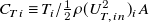
 \begin{equation} \chi \equiv \frac {\langle U_{T,in}\rangle }{U_F},\hspace {12pt} \chi _T \equiv \frac {\langle U_{T,in}^2\rangle }{U_F^2} = \frac {C_T^*}{C_T},\hspace {12pt} \chi _P \equiv \frac {\langle U_{T,in}^3\rangle }{U_F^3} = \frac {C_P^*}{C_P}, \end{equation}
where
 $\chi _T$
and
$\chi _T$
and
 $\chi _P$
are the layout factors to be modelled for the thrust and power, respectively, and
$\chi _P$
are the layout factors to be modelled for the thrust and power, respectively, and
 $C_T$
is the ‘effective’ thrust coefficient of all individual turbines in the farm, i.e.
$C_T$
is the ‘effective’ thrust coefficient of all individual turbines in the farm, i.e.
 $C_T \equiv \langle T \rangle / \frac {1}{2}\rho \langle U_{T,in}^2\rangle A$
, where
$C_T \equiv \langle T \rangle / \frac {1}{2}\rho \langle U_{T,in}^2\rangle A$
, where
 $\langle T \rangle \equiv \Sigma _{i=1}^N T_i/N$
is the farm-averaged value of the turbine thrust. Similarly to the ‘effective’ power coefficient
$\langle T \rangle \equiv \Sigma _{i=1}^N T_i/N$
is the farm-averaged value of the turbine thrust. Similarly to the ‘effective’ power coefficient
 $C_P$
defined earlier in (3.1), this
$C_P$
defined earlier in (3.1), this
 $C_T$
is identical to the thrust coefficient of each individual turbine,
$C_T$
is identical to the thrust coefficient of each individual turbine,
 $C_{Ti}\equiv T_i/\frac {1}{2}\rho (U_{T,in}^2)_iA$
, if all turbines in the farm have the same
$C_{Ti}\equiv T_i/\frac {1}{2}\rho (U_{T,in}^2)_iA$
, if all turbines in the farm have the same
 $C_{Ti}$
value. Note that
$C_{Ti}$
value. Note that
 $\chi _T$
affects
$\chi _T$
affects
 $\beta$
(via the NDFM equation) and thus
$\beta$
(via the NDFM equation) and thus
 $\eta _{\textrm {ext}}$
, whereas
$\eta _{\textrm {ext}}$
, whereas
 $\chi _P$
decides
$\chi _P$
decides
 $\eta _{\textrm {int}}$
, and in general, the relationships among
$\eta _{\textrm {int}}$
, and in general, the relationships among
 $\chi$
,
$\chi$
,
 $\chi _T$
and
$\chi _T$
and
 $\chi _P$
are unknown (as they depend on the variation of
$\chi _P$
are unknown (as they depend on the variation of
 $U_{T,in}$
in a given farm). However, in special cases where most turbines have approximately the same inflow speed, e.g. when the turbine array is homogeneous and the farm is large enough for the internal boundary layer to be fully developed for most of the farm, we obtain
$U_{T,in}$
in a given farm). However, in special cases where most turbines have approximately the same inflow speed, e.g. when the turbine array is homogeneous and the farm is large enough for the internal boundary layer to be fully developed for most of the farm, we obtain
 $\chi _T\approx \chi ^2$
and
$\chi _T\approx \chi ^2$
and
 $\chi _P\approx \chi ^3$
, and hence,
$\chi _P\approx \chi ^3$
, and hence,
 $\chi _P\approx \chi _T^{3/2}$
.
$\chi _P\approx \chi _T^{3/2}$
.
The definitions of the power coefficients, efficiencies and layout factors introduced above are generic and compatible with the core framework of the two-scale momentum theory summarised in § 2.1, requiring no assumption on the spatio-temporal variation of the flow field (such as scale separation).
3.2. Modelling of turbine layout factors
As noted in § 2.3, recent studies (Legris et al. Reference Legris, Pahus, Nishino and Perez-Campos2023; Pahus et al. Reference Pahus, Nishino, Kirby and Vogel2024) show that an engineering wake model can predict turbine layout effects on
 $C_T^*$
numerically for a given wind farm. However, since our aim here is to provide a holistic view of wind farm power performance, we need an analytical model that allows us to predict
$C_T^*$
numerically for a given wind farm. However, since our aim here is to provide a holistic view of wind farm power performance, we need an analytical model that allows us to predict
 $C_T^*$
(and
$C_T^*$
(and
 $C_P^*$
) instantly for a range of conditions, most importantly for different values of turbine spacing and thrust coefficient. In the following, we propose a basic model of the layout factor
$C_P^*$
) instantly for a range of conditions, most importantly for different values of turbine spacing and thrust coefficient. In the following, we propose a basic model of the layout factor
 $\chi$
that resembles an engineering wake model, but incorporates an empirical parameter that can be tuned with LES data. Note that the scale separation assumption (ND20, see also Kirby et al. Reference Kirby, Nishino, Lanzilao, Dunstan and Meyers2025) is adopted here and in § 3.3, i.e. we assume that
$\chi$
that resembles an engineering wake model, but incorporates an empirical parameter that can be tuned with LES data. Note that the scale separation assumption (ND20, see also Kirby et al. Reference Kirby, Nishino, Lanzilao, Dunstan and Meyers2025) is adopted here and in § 3.3, i.e. we assume that
 $\chi$
,
$\chi$
,
 $\chi _T$
,
$\chi _T$
,
 $\chi _P(=\eta _{\textrm {int}})$
and
$\chi _P(=\eta _{\textrm {int}})$
and
 $\eta _{\textrm {rot}}$
are ‘internal’ parameters, and therefore not directly affected by ‘external’ flow conditions, such as the ABL height.
$\eta _{\textrm {rot}}$
are ‘internal’ parameters, and therefore not directly affected by ‘external’ flow conditions, such as the ABL height.
Kirby et al. (Reference Kirby, Nishino and Dunstan2022) performed 50 different cases of LES of a neutral ABL over a regular periodic array of actuator discs with
 $C_T'=1.33$
(which corresponds to
$C_T'=1.33$
(which corresponds to
 $C_T=0.75$
) for a range of turbine spacing (
$C_T=0.75$
) for a range of turbine spacing (
 $5D\le s_x \le 10D$
and
$5D\le s_x \le 10D$
and
 $5D \le s_y \le 10D$
) and wind direction (
$5D \le s_y \le 10D$
) and wind direction (
 $0^{\circ } \le \theta \lt 45^{\circ }$
). The values of
$0^{\circ } \le \theta \lt 45^{\circ }$
). The values of
 $\chi _T$
computed from the 50 LES cases are plotted in Figure 2a against the non-dimensional average turbine spacing
$\chi _T$
computed from the 50 LES cases are plotted in Figure 2a against the non-dimensional average turbine spacing
 $\sqrt {s_xs_y}/D=\sqrt {S_F/ND^2}$
for five sub-ranges of
$\sqrt {s_xs_y}/D=\sqrt {S_F/ND^2}$
for five sub-ranges of
 $\theta$
. It is clear that
$\theta$
. It is clear that
 $\chi _T$
is close to 1 for the majority of the 50 cases, but decreases to approximately 0.8 when
$\chi _T$
is close to 1 for the majority of the 50 cases, but decreases to approximately 0.8 when
 $\theta$
is close to
$\theta$
is close to
 $0^{\circ }$
, i.e. when the wind direction is close to one of the two axes of the regular array, causing significant wake interference. These
$0^{\circ }$
, i.e. when the wind direction is close to one of the two axes of the regular array, causing significant wake interference. These
 $\chi _T$
values are almost identical to the values of
$\chi _T$
values are almost identical to the values of
 $\chi _P^{2/3}$
, as shown in Figure 2b for the same 50 LES cases, since the inflow speed
$\chi _P^{2/3}$
, as shown in Figure 2b for the same 50 LES cases, since the inflow speed
 $U_{T,in}$
is almost the same for all turbines in each regular periodic array simulated. Although real wind farms may have a variation of
$U_{T,in}$
is almost the same for all turbines in each regular periodic array simulated. Although real wind farms may have a variation of
 $U_{T,in}$
, here, we assume
$U_{T,in}$
, here, we assume
 $\chi _T = \chi ^2$
and
$\chi _T = \chi ^2$
and
 $\chi _P = \chi ^3$
for simplicity and propose a single model of
$\chi _P = \chi ^3$
for simplicity and propose a single model of
 $\chi$
that can reproduce the layout effects observed in these LES data. Note that when the variation of
$\chi$
that can reproduce the layout effects observed in these LES data. Note that when the variation of
 $U_{T,in}$
is large, we would need to either (i) introduce an additional model parameter to account for the variance of
$U_{T,in}$
is large, we would need to either (i) introduce an additional model parameter to account for the variance of
 $U_{T,in}$
, or (ii) calculate
$U_{T,in}$
, or (ii) calculate
 $\chi _T$
and
$\chi _T$
and
 $\chi _P$
directly from the results of numerical simulations for a given layout. However, this is outside the scope of the present study.
$\chi _P$
directly from the results of numerical simulations for a given layout. However, this is outside the scope of the present study.
Turbine layout factors and the model parameter
 $C_{\chi }$
computed from the LES results reported by Kirby et al. (Reference Kirby, Nishino and Dunstan2022) for 50 different periodic arrays of actuator discs: (a)
$C_{\chi }$
computed from the LES results reported by Kirby et al. (Reference Kirby, Nishino and Dunstan2022) for 50 different periodic arrays of actuator discs: (a)
 $\chi _T$
plotted against the non-dimensional average turbine spacing for five different sub-ranges of wind direction; (b) comparison of
$\chi _T$
plotted against the non-dimensional average turbine spacing for five different sub-ranges of wind direction; (b) comparison of
 $\chi _T$
and
$\chi _T$
and
 $\chi _P^{2/3}$
; and (c) the parameter
$\chi _P^{2/3}$
; and (c) the parameter
 $C_{\chi }$
for the proposed model, (3.6).
$C_{\chi }$
for the proposed model, (3.6).

The LES results plotted in Figure 2a do not show a clear dependency of
 $\chi _T$
on the turbine spacing, but theoretically,
$\chi _T$
on the turbine spacing, but theoretically,
 $\chi$
,
$\chi$
,
 $\chi _T$
and
$\chi _T$
and
 $\chi _P$
should all converge to 1 as the turbine spacing becomes very large and all flow interaction effects diminish. Also, these LES results are for a given
$\chi _P$
should all converge to 1 as the turbine spacing becomes very large and all flow interaction effects diminish. Also, these LES results are for a given
 $C_T$
value (0.75), but
$C_T$
value (0.75), but
 $\chi$
,
$\chi$
,
 $\chi _T$
and
$\chi _T$
and
 $\chi _P$
should all converge to 1 as
$\chi _P$
should all converge to 1 as
 $C_T$
approaches zero. Since the dependency of
$C_T$
approaches zero. Since the dependency of
 $\chi$
on
$\chi$
on
 $C_T$
and turbine spacing is expected to be similar to how the wind speed behind a single turbine depends on its
$C_T$
and turbine spacing is expected to be similar to how the wind speed behind a single turbine depends on its
 $C_T$
and streamwise distance, we adopt the formulation of the traditional wake model of Jensen (Reference Jensen1983) and Katić et al. (Reference Katić, Højstrup and Jensen1986), and introduce a model parameter
$C_T$
and streamwise distance, we adopt the formulation of the traditional wake model of Jensen (Reference Jensen1983) and Katić et al. (Reference Katić, Højstrup and Jensen1986), and introduce a model parameter
 $C_\chi$
to formulate our analytical model of
$C_\chi$
to formulate our analytical model of
 $\chi$
as
$\chi$
as
 \begin{equation} \chi = \chi _T^{1/2} = \chi _P^{1/3} = 1-C_{\chi }\left [ \frac {1-\sqrt {1-C_T}}{( 1+2k\sqrt {\pi /4\lambda } )^2} \right ], \end{equation}
where the term inside the square brackets represents the ‘wake deficit’ expected at a distance
 $D\sqrt {\pi /4\lambda }$
downstream of a given turbine and
$D\sqrt {\pi /4\lambda }$
downstream of a given turbine and
 $k=0.05$
is a typical wake growth rate (Porté-Agel et al. Reference Porté-Agel, Bastankhah and Shamsoddin2020). Note that
$k=0.05$
is a typical wake growth rate (Porté-Agel et al. Reference Porté-Agel, Bastankhah and Shamsoddin2020). Note that
 $D\sqrt {\pi /4\lambda }=\sqrt {S_F/N}=\sqrt {s_xs_y}$
is the average turbine spacing in a farm. This means that
$D\sqrt {\pi /4\lambda }=\sqrt {S_F/N}=\sqrt {s_xs_y}$
is the average turbine spacing in a farm. This means that
 $C_\chi \approx 1$
is expected when the wind direction is perfectly aligned with an axis of a regular array of turbines with
$C_\chi \approx 1$
is expected when the wind direction is perfectly aligned with an axis of a regular array of turbines with
 $s_x=s_y$
(because the value of
$s_x=s_y$
(because the value of
 $\chi \equiv \langle U_{T,in}\rangle /U_F$
should be similar to the ‘wake deficit’ at
$\chi \equiv \langle U_{T,in}\rangle /U_F$
should be similar to the ‘wake deficit’ at
 $D\sqrt {\pi /4\lambda }$
downstream of a turbine in such a special case), whereas
$D\sqrt {\pi /4\lambda }$
downstream of a turbine in such a special case), whereas
 $C_\chi \approx 0$
is expected when the wind direction is such that there is little wake interference. In other words, this parameter
$C_\chi \approx 0$
is expected when the wind direction is such that there is little wake interference. In other words, this parameter
 $C_\chi$
should depend largely on the degree of ‘overlap’ of rotor areas projected in the wind direction (noting that a similar concept of ‘overlap’ has been adopted by, e.g. Ghaisas and Archer (Reference Ghaisas and Archer2016)). This is confirmed by calculating
$C_\chi$
should depend largely on the degree of ‘overlap’ of rotor areas projected in the wind direction (noting that a similar concept of ‘overlap’ has been adopted by, e.g. Ghaisas and Archer (Reference Ghaisas and Archer2016)). This is confirmed by calculating
 $C_\chi$
directly from the LES results, i.e. by substituting the LES results of
$C_\chi$
directly from the LES results, i.e. by substituting the LES results of
 $\chi _T$
shown in Figure 2a into (3.6) together with the value of
$\chi _T$
shown in Figure 2a into (3.6) together with the value of
 $C_T$
and the average turbine spacing. The
$C_T$
and the average turbine spacing. The
 $C_\chi$
values calculated are plotted in Figure 2c for all 50 LES cases, showing that
$C_\chi$
values calculated are plotted in Figure 2c for all 50 LES cases, showing that
 $C_\chi \lt 0.5$
for most cases. Although there is scatter due to combined effects of the turbine layout (
$C_\chi \lt 0.5$
for most cases. Although there is scatter due to combined effects of the turbine layout (
 $s_x$
and
$s_x$
and
 $s_y$
) and wind direction, we can see the trend that
$s_y$
) and wind direction, we can see the trend that
 $C_\chi$
increases when
$C_\chi$
increases when
 $\theta$
approaches
$\theta$
approaches
 $0^\circ$
(at which the turbine rows are fully aligned) and
$0^\circ$
(at which the turbine rows are fully aligned) and
 $45^\circ$
(at which the turbines are diagonally aligned if
$45^\circ$
(at which the turbines are diagonally aligned if
 $s_x \approx s_y$
).
$s_x \approx s_y$
).
Note that
 $C_{\chi }$
may take a small negative value since, depending on the wind direction, the average turbine inflow speed
$C_{\chi }$
may take a small negative value since, depending on the wind direction, the average turbine inflow speed
 $\langle U_{T,in}\rangle$
may become slightly higher than
$\langle U_{T,in}\rangle$
may become slightly higher than
 $U_F$
due to local flow acceleration; see Kirby et al. (Reference Kirby, Nishino and Dunstan2022) for further details. Such flow acceleration cannot be predicted by the superposition of engineering wake models, suggesting the advantage of using LES data to estimate
$U_F$
due to local flow acceleration; see Kirby et al. (Reference Kirby, Nishino and Dunstan2022) for further details. Such flow acceleration cannot be predicted by the superposition of engineering wake models, suggesting the advantage of using LES data to estimate
 $C_\chi$
, which captures the combined effects of
$C_\chi$
, which captures the combined effects of
 $s_x$
,
$s_x$
,
 $s_y$
and
$s_y$
and
 $\theta$
in the case of a regular array. Strictly speaking,
$\theta$
in the case of a regular array. Strictly speaking,
 $C_\chi$
may also be affected by
$C_\chi$
may also be affected by
 $C_T$
and
$C_T$
and
 $\lambda$
, but the assumption here is that the effects of
$\lambda$
, but the assumption here is that the effects of
 $C_T$
and
$C_T$
and
 $\lambda$
are mostly captured by the term inside the square brackets in (3.6). This allows us to analytically explore the optimal farm induction factor and the optimal thrust coefficient required to maximise the farm power later in § 4.2.
$\lambda$
are mostly captured by the term inside the square brackets in (3.6). This allows us to analytically explore the optimal farm induction factor and the optimal thrust coefficient required to maximise the farm power later in § 4.2.
The simple analytical formulation of
 $\chi$
in (3.6) is largely motivated by the scarcity of wind farm LES data available for empirical tuning. If sufficient LES data were available not only for a range of turbine layouts and wind directions, but also for a range of
$\chi$
in (3.6) is largely motivated by the scarcity of wind farm LES data available for empirical tuning. If sufficient LES data were available not only for a range of turbine layouts and wind directions, but also for a range of
 $C_T$
, it would be possible to develop a data-driven model of
$C_T$
, it would be possible to develop a data-driven model of
 $\chi$
as a function of
$\chi$
as a function of
 $C_T$
, wind direction and turbine layout, without relying on the formulation taken from an engineering wake model to capture the dependency of
$C_T$
, wind direction and turbine layout, without relying on the formulation taken from an engineering wake model to capture the dependency of
 $\chi$
on
$\chi$
on
 $C_T$
. It should also be noted that the LES data used here are for infinitely large wind farms and hence, there is a possibility that
$C_T$
. It should also be noted that the LES data used here are for infinitely large wind farms and hence, there is a possibility that
 $C_{\chi }$
in Figure 2c may have been under-predicted. However, the finite-size wind farm LES results by Kirby et al. (Reference Kirby, Nishino, Lanzilao, Dunstan and Meyers2025) suggest that
$C_{\chi }$
in Figure 2c may have been under-predicted. However, the finite-size wind farm LES results by Kirby et al. (Reference Kirby, Nishino, Lanzilao, Dunstan and Meyers2025) suggest that
 $C_T^*$
is insensitive to the farm size, meaning that the results in Figure 2c should be applicable to large finite-size wind farms. More LES data for finite-size wind farms would be required to fully confirm this in future studies.
$C_T^*$
is insensitive to the farm size, meaning that the results in Figure 2c should be applicable to large finite-size wind farms. More LES data for finite-size wind farms would be required to fully confirm this in future studies.
Although
 $C_{\chi }$
depends significantly on the wind direction, in this study, we will adopt (unless stated otherwise)
$C_{\chi }$
depends significantly on the wind direction, in this study, we will adopt (unless stated otherwise)
 $C_{\chi }=0.14$
, the average value of all 50 LES results shown in Figure 2c for the purpose of demonstration. Note that these 50 cases cover a typical range of layout parameter space (
$C_{\chi }=0.14$
, the average value of all 50 LES results shown in Figure 2c for the purpose of demonstration. Note that these 50 cases cover a typical range of layout parameter space (
 $s_x$
,
$s_x$
,
 $s_y$
,
$s_y$
,
 $\theta$
) in an unbiased manner, representing a general set of layout scenarios; hence, this
$\theta$
) in an unbiased manner, representing a general set of layout scenarios; hence, this
 $C_{\chi }=0.14$
can be seen as a typical value for large offshore wind farms (with an average turbine spacing of between
$C_{\chi }=0.14$
can be seen as a typical value for large offshore wind farms (with an average turbine spacing of between
 $5D$
and
$5D$
and
 $10D$
). In reality, however, it is common that there is a dominant wind direction at a given site and wind farm developers ensure that the axes of their turbine array are not aligned with that direction (e.g. by having a slightly irregular array configuration), meaning that the average value of
$10D$
). In reality, however, it is common that there is a dominant wind direction at a given site and wind farm developers ensure that the axes of their turbine array are not aligned with that direction (e.g. by having a slightly irregular array configuration), meaning that the average value of
 $C_{\chi }$
could be lower. In addition, some flow control techniques to reduce turbine–wake interference, such as ‘wake steering’ (Fleming et al. Reference Fleming, Annoni, Shah, Wang, Ananthan, Zhang, Hutchings, Wang, Chen and Chen2017; Howland et al. Reference Howland, Lele and Dabiri2019), could lower the average value of
$C_{\chi }$
could be lower. In addition, some flow control techniques to reduce turbine–wake interference, such as ‘wake steering’ (Fleming et al. Reference Fleming, Annoni, Shah, Wang, Ananthan, Zhang, Hutchings, Wang, Chen and Chen2017; Howland et al. Reference Howland, Lele and Dabiri2019), could lower the average value of
 $C_{\chi }$
even further.
$C_{\chi }$
even further.
Comparison of standard
 $C_P$
versus
$C_P$
versus
 $C_T$
curves for three reference wind turbine models (purple) with the classical ADT (blue) and the proposed analytical model (green): (a) DTU 10 MW turbine; (b) IEA 10 MW turbine; and (c) IEA 15 MW turbine. The square symbols show the rated operating points.
$C_T$
curves for three reference wind turbine models (purple) with the classical ADT (blue) and the proposed analytical model (green): (a) DTU 10 MW turbine; (b) IEA 10 MW turbine; and (c) IEA 15 MW turbine. The square symbols show the rated operating points.

3.3. Modelling of rotor efficiency
The rotor efficiency
 $\eta _{\textrm {rot}}$
can be predicted by the classical BEM theory as a function of the rotor design and operating conditions (such as the blade pitch angle and the tip-speed ratio). Using the BEM theory together with the two-scale momentum theory would enable optimisation of the design and operation of wind turbines and wind farms in a coupled manner (Nishino & Hunter Reference Nishino and Hunter2018). However, since our focus here is on wind farm performance and we prefer to keep this theoretical farm model as simple as possible, we introduce an analytical model of
$\eta _{\textrm {rot}}$
can be predicted by the classical BEM theory as a function of the rotor design and operating conditions (such as the blade pitch angle and the tip-speed ratio). Using the BEM theory together with the two-scale momentum theory would enable optimisation of the design and operation of wind turbines and wind farms in a coupled manner (Nishino & Hunter Reference Nishino and Hunter2018). However, since our focus here is on wind farm performance and we prefer to keep this theoretical farm model as simple as possible, we introduce an analytical model of
 $\eta _{\textrm {rot}}$
that requires only the rated thrust coefficient,
$\eta _{\textrm {rot}}$
that requires only the rated thrust coefficient,
 $C_T^{\textrm {Rat}}$
, and rated power coefficient,
$C_T^{\textrm {Rat}}$
, and rated power coefficient,
 $C_P^{\textrm {Rat}}$
, of real turbines as input. Specifically, we use
$C_P^{\textrm {Rat}}$
, of real turbines as input. Specifically, we use
 $C_T^{\textrm {Rat}}$
and
$C_T^{\textrm {Rat}}$
and
 $C_P^{\textrm {Rat}}$
to correct the power coefficient of aerodynamically ideal turbines,
$C_P^{\textrm {Rat}}$
to correct the power coefficient of aerodynamically ideal turbines,
 $C_{P,\textrm {ADT}}$
, to estimate
$C_{P,\textrm {ADT}}$
, to estimate
 $C_P$
as follows:
$C_P$
as follows:
 \begin{equation} C_P = \eta _{\textrm {rot}}C_{P,\textrm {ADT}} = \left [ \frac {\sigma C_P^{\textrm {Rat}}+(1-\sigma ) C_{P,\textrm {ADT}}^{\textrm { Rat}}}{C_{P,\textrm {ADT}}^{\textrm {Rat}}}\right ] C_{P,\textrm {ADT}}, \end{equation}
where
 \begin{equation} C_{P,\textrm {ADT}} = \frac {1}{2}C_T\left (1+\sqrt {1-C_T} \right ), \hspace {10pt} C_{P,\textrm {ADT}}^{\textrm {Rat}} = \frac {1}{2}C_T^{\textrm {Rat}}\left (1+\sqrt {1-C_T^{\textrm {Rat}}} \right ), \hspace {10pt} \sigma = \left ( \frac {\frac {C_T}{C_{P,\textrm {ADT}}}-1}{\frac {C_T^{\textrm {Rat}}}{C_{P,\textrm {ADT}}^{\textrm {Rat}}}-1} \right )^{\frac {1}{2}}. \end{equation}
Here, the model parameter
 $\sigma$
has been designed to increase exponentially from 0 to 1 (and hence,
$\sigma$
has been designed to increase exponentially from 0 to 1 (and hence,
 $\eta _{\textrm {rot}}$
decreases from 1 to
$\eta _{\textrm {rot}}$
decreases from 1 to
 $C_P^{\textrm {Rat}}/C_{P,\textrm {ADT}}^{\textrm {Rat}}$
) as
$C_P^{\textrm {Rat}}/C_{P,\textrm {ADT}}^{\textrm {Rat}}$
) as
 $C_T$
increases from 0 to
$C_T$
increases from 0 to
 $C_T^{\textrm {Rat}}$
, noting that the value of
$C_T^{\textrm {Rat}}$
, noting that the value of
 $C_T/C_{P,\textrm {ADT}}$
approaches 1 as
$C_T/C_{P,\textrm {ADT}}$
approaches 1 as
 $C_T$
approaches 0. The exponent ‘1/2’ in the formulation of
$C_T$
approaches 0. The exponent ‘1/2’ in the formulation of
 $\sigma$
has been determined empirically. Figure 3 shows comparisons of this simple analytical model with ‘standard’
$\sigma$
has been determined empirically. Figure 3 shows comparisons of this simple analytical model with ‘standard’
 $C_P$
versus
$C_P$
versus
 $C_T$
curves for the DTU 10 MW, IEA 10 MW and IEA 15 MW reference turbines, confirming that the model agrees well with these ‘real’ rotor performance curves for the whole range of
$C_T$
curves for the DTU 10 MW, IEA 10 MW and IEA 15 MW reference turbines, confirming that the model agrees well with these ‘real’ rotor performance curves for the whole range of
 $C_T$
up to the rated
$C_T$
up to the rated
 $C_T$
. Note that the sudden drop of
$C_T$
. Note that the sudden drop of
 $C_P$
above the rated
$C_P$
above the rated
 $C_T$
cannot be predicted by this simple analytical model, but this drop corresponds to the degradation of rotor efficiency at low wind speeds, at which the operating conditions of these rotors are not aerodynamically optimal. A very similar type of analytical rotor efficiency model has also been proposed by van der Laan et al. (Reference van der Laan, Andersen, Réthoré, Baungaard, Sørensen and Troldborg2022) and validated for a wider range of common wind turbine rotors, showing the same trend as the model proposed here.
$C_T$
cannot be predicted by this simple analytical model, but this drop corresponds to the degradation of rotor efficiency at low wind speeds, at which the operating conditions of these rotors are not aerodynamically optimal. A very similar type of analytical rotor efficiency model has also been proposed by van der Laan et al. (Reference van der Laan, Andersen, Réthoré, Baungaard, Sørensen and Troldborg2022) and validated for a wider range of common wind turbine rotors, showing the same trend as the model proposed here.
4. Examples of solutions
Now, we present some examples of the solutions obtained from the two-scale theory and its analytical sub-models described above. The key assumptions required are as follows.
-
• We consider an offshore or flat onshore wind farm (so that the theory described in §§ 2.1 and 3.1 is applicable).
-
• The farm length is at least an order of magnitude larger than the ABL height (so that the analytical model of
$M$
in § 2.2 is applicable). -
• All turbines have the same rotor design, blade angle and tip-speed ratio (so that the rotor efficiency model in § 3.3 can be used to estimate
$C_P$
as a function of
$C_T$
). -
• The inflow speed
$U_{T,in}$
is approximately the same for most turbines (so that the layout factor model in § 3.2 can be used to estimate
$\chi _T$
and
$\chi _P$
as a function of
$C_T$
,
$\lambda$
and
$C_\chi$
).


Note that the second condition is not fully satisfied for two of the five ‘onshore’ cases in § 4.3, where the ABL height
 $h_0$
is larger than
$h_0$
is larger than
 $10\,\%$
of the farm length
$10\,\%$
of the farm length
 $L$
. Also note that the fourth condition is not required if
$L$
. Also note that the fourth condition is not required if
 $\chi _T$
and
$\chi _T$
and
 $\chi _P$
are calculated directly from numerical simulations.
$\chi _P$
are calculated directly from numerical simulations.
4.1. Relationship between
$\beta$
and
$C_{PG}$


First, we present the farm wind-speed reduction factor
 $\beta$
(obtained from the NDFM equation (2.2) with the model of
$\beta$
(obtained from the NDFM equation (2.2) with the model of
 $M$
in (2.10)) and the global power coefficient
$M$
in (2.10)) and the global power coefficient
 $C_{PG}$
 $(=\eta _{\textrm {ext}}\eta _{\textrm {int}}\eta _{\textrm { rot}}C_{P,\textrm {ADT}})$
in Figures 4 and 5 for idealised and realistic farms, respectively, for a range of effective array density (
$(=\eta _{\textrm {ext}}\eta _{\textrm {int}}\eta _{\textrm { rot}}C_{P,\textrm {ADT}})$
in Figures 4 and 5 for idealised and realistic farms, respectively, for a range of effective array density (
 $\lambda /C_{f0}=5, 10, 15$
) and effective ABL height (
$\lambda /C_{f0}=5, 10, 15$
) and effective ABL height (
 $h_0/LC_{f0}=10, 15, 20$
). Also presented together in Figure 5 are the internal power coefficient
$h_0/LC_{f0}=10, 15, 20$
). Also presented together in Figure 5 are the internal power coefficient
 $C_P^*$
 $(=\eta _{\textrm {int}}\eta _{\textrm {rot}}C_{P,\textrm {ADT}})$
and the effective turbine power coefficient
$(=\eta _{\textrm {int}}\eta _{\textrm {rot}}C_{P,\textrm {ADT}})$
and the effective turbine power coefficient
 $C_P$
$C_P$
 $(=\eta _{\textrm {rot}}C_{P,\textrm {ADT}})$
. For a typical offshore case with
$(=\eta _{\textrm {rot}}C_{P,\textrm {ADT}})$
. For a typical offshore case with
 $C_{f0}=0.002$
, these
$C_{f0}=0.002$
, these
 $\lambda /C_{f0}$
values correspond to the average turbine spacing of approximately
$\lambda /C_{f0}$
values correspond to the average turbine spacing of approximately
 $8.9D$
,
$8.9D$
,
 $6.3D$
and
$6.3D$
and
 $5.1D$
, respectively. In addition, if we assume that the farm length
$5.1D$
, respectively. In addition, if we assume that the farm length
 $L$
is 20 km, these
$L$
is 20 km, these
 $h_0/LC_{f0}$
values would correspond to typical offshore ABL heights of 0.4, 0.6 and 0.8 km, respectively. Both figures demonstrate some general trends: (i)
$h_0/LC_{f0}$
values would correspond to typical offshore ABL heights of 0.4, 0.6 and 0.8 km, respectively. Both figures demonstrate some general trends: (i)
 $\beta$
decreases (i.e. farm-average wind speed decreases) as
$\beta$
decreases (i.e. farm-average wind speed decreases) as
 $C_T$
increases; (ii) for a given wind farm, there is an optimal
$C_T$
increases; (ii) for a given wind farm, there is an optimal
 $C_T$
and thus an optimal
$C_T$
and thus an optimal
 $\beta$
that maximise
$\beta$
that maximise
 $C_{PG}$
; and (iii) for a given
$C_{PG}$
; and (iii) for a given
 $C_T$
, both
$C_T$
, both
 $\beta$
and
$\beta$
and
 $C_{PG}$
decrease as the effective array density (
$C_{PG}$
decrease as the effective array density (
 $\lambda /C_{f0}$
) increases and/or the effective ABL height (
$\lambda /C_{f0}$
) increases and/or the effective ABL height (
 $h_0/LC_{f0}$
) decreases. The trend of the impact of the array density observed here is the same as that predicted by the classical top-down models (see, e.g. Stevens et al. (Reference Stevens, Gayme and Meneveau2016) and references cited therein).
$h_0/LC_{f0}$
) decreases. The trend of the impact of the array density observed here is the same as that predicted by the classical top-down models (see, e.g. Stevens et al. (Reference Stevens, Gayme and Meneveau2016) and references cited therein).
The efficiency of an idealised wind farm (
 $\eta _{\textrm {rot}}=\chi _T=\chi _P=1$
) with different effective array densities (
$\eta _{\textrm {rot}}=\chi _T=\chi _P=1$
) with different effective array densities (
 $\lambda /C_{f0}$
) and effective ABL heights (
$\lambda /C_{f0}$
) and effective ABL heights (
 $h_0/LC_{f0}$
). Solid lines,
$h_0/LC_{f0}$
). Solid lines,
 $h_0/LC_{f0}=20$
. Dashed lines,
$h_0/LC_{f0}=20$
. Dashed lines,
 $h_0/LC_{f0}=15$
. Dash-dotted lines,
$h_0/LC_{f0}=15$
. Dash-dotted lines,
 $h_0/LC_{f0}=10$
.
$h_0/LC_{f0}=10$
.

Efficiency of a realistic wind farm with IEA 15 MW turbines (
 $C_T^{\rm {Rat}}=0.8$
,
$C_T^{\rm {Rat}}=0.8$
,
 $C_P^{\rm {Rat}}=0.489$
) for a typical offshore scenario (
$C_P^{\rm {Rat}}=0.489$
) for a typical offshore scenario (
 $C_{f0}=0.002$
,
$C_{f0}=0.002$
,
 $C_\chi =0.14$
) with different values of
$C_\chi =0.14$
) with different values of
 $\lambda /C_{f0}$
and
$\lambda /C_{f0}$
and
 $h_0/LC_{f0}$
. Solid lines,
$h_0/LC_{f0}$
. Solid lines,
 $h_0/LC_{f0}=20$
. Dashed lines,
$h_0/LC_{f0}=20$
. Dashed lines,
 $h_0/LC_{f0}=15$
. Dash-dotted lines,
$h_0/LC_{f0}=15$
. Dash-dotted lines,
 $h_0/LC_{f0}=10$
.
$h_0/LC_{f0}=10$
.

Note that the ratio of
 $C_{PG}$
to
$C_{PG}$
to
 $C_{P,\textrm {ADT}}$
in Figure 4 is the ‘external’ efficiency
$C_{P,\textrm {ADT}}$
in Figure 4 is the ‘external’ efficiency
 $\eta _{\textrm {ext}}$
(
$\eta _{\textrm {ext}}$
(
 $=\beta ^3$
) since there is no other power loss in these idealised cases (
$=\beta ^3$
) since there is no other power loss in these idealised cases (
 $C_{P,\textrm {ADT}}=C_P=C_P^*$
and thus
$C_{P,\textrm {ADT}}=C_P=C_P^*$
and thus
 $\eta _{\textrm {rot}}=\eta _{\textrm {int}}=1$
). For these idealised wind farms,
$\eta _{\textrm {rot}}=\eta _{\textrm {int}}=1$
). For these idealised wind farms,
 $\eta _{\textrm {ext}}$
is equivalent to
$\eta _{\textrm {ext}}$
is equivalent to
 $\eta _{FS}$
proposed by Kirby et al. (Reference Kirby, Nishino, Lanzilao, Dunstan and Meyers2025). However, in realistic wind farms (Figure 5), there are power losses due to rotor design (i.e.
$\eta _{FS}$
proposed by Kirby et al. (Reference Kirby, Nishino, Lanzilao, Dunstan and Meyers2025). However, in realistic wind farms (Figure 5), there are power losses due to rotor design (i.e.
 $C_{P,\textrm {ADT}}\gt C_P$
) and direct wake interference (i.e.
$C_{P,\textrm {ADT}}\gt C_P$
) and direct wake interference (i.e.
 $C_P\gt C_P^*$
). Since
$C_P\gt C_P^*$
). Since
 $C_T^*$
also decreases from
$C_T^*$
also decreases from
 $C_T$
due to direct wake interference,
$C_T$
due to direct wake interference,
 $\beta$
is slightly higher in Figure 5 than in Figure 4, meaning that
$\beta$
is slightly higher in Figure 5 than in Figure 4, meaning that
 $\eta _{\textrm {ext}}$
is higher in the realistic case than in the idealised case, even though
$\eta _{\textrm {ext}}$
is higher in the realistic case than in the idealised case, even though
 $C_{PG}$
is lower in the realistic case. It is therefore important to note that, for realistic wind farms,
$C_{PG}$
is lower in the realistic case. It is therefore important to note that, for realistic wind farms,
 $\eta _{\textrm {ext}}$
is different from
$\eta _{\textrm {ext}}$
is different from
 $\eta _{FS}$
proposed by Kirby et al. (Reference Kirby, Nishino, Lanzilao, Dunstan and Meyers2025). Nonetheless, the new theoretical results in Figure 5 show that, for this example of a large offshore wind farm with
$\eta _{FS}$
proposed by Kirby et al. (Reference Kirby, Nishino, Lanzilao, Dunstan and Meyers2025). Nonetheless, the new theoretical results in Figure 5 show that, for this example of a large offshore wind farm with
 $C_\chi =0.14$
, the power loss due to ‘farm–atmosphere interactions’ (or the reduction of the farm-average wind speed) can still be the largest part of the overall power losses. In Figure 5, the reduction from
$C_\chi =0.14$
, the power loss due to ‘farm–atmosphere interactions’ (or the reduction of the farm-average wind speed) can still be the largest part of the overall power losses. In Figure 5, the reduction from
 $C_P^*$
to
$C_P^*$
to
 $C_{PG}$
(due to ‘external’ flow interactions) is larger than the reduction from
$C_{PG}$
(due to ‘external’ flow interactions) is larger than the reduction from
 $C_P$
to
$C_P$
to
 $C_P^*$
(due to ‘internal’ flow interactions) for the typical ranges of the array density and the ABL height considered.
$C_P^*$
(due to ‘internal’ flow interactions) for the typical ranges of the array density and the ABL height considered.
4.2. Iterative solution for optimal
$\beta$
and
$C_T$


Of interest here is how the optimal
 $C_T$
that maximises
$C_T$
that maximises
 $C_{PG}$
changes with various factors. In contrast to
$C_{PG}$
changes with various factors. In contrast to
 $C_{P,\textrm {ADT}}$
, which always takes the maximum value of
$C_{P,\textrm {ADT}}$
, which always takes the maximum value of
 $16/27\approx 0.593$
(the Betz limit) at a high optimal
$16/27\approx 0.593$
(the Betz limit) at a high optimal
 $C_T$
value of
$C_T$
value of
 $8/9\approx 0.889$
, the farm power is maximised at a lower optimal
$8/9\approx 0.889$
, the farm power is maximised at a lower optimal
 $C_T$
value that depends on
$C_T$
value that depends on
 $\lambda /C_{f0}$
and
$\lambda /C_{f0}$
and
 $h_0/LC_{f0}$
as well as on the rotor design and turbine layout factors. If
$h_0/LC_{f0}$
as well as on the rotor design and turbine layout factors. If
 $C_T$
is set higher than this optimal value,
$C_T$
is set higher than this optimal value,
 $C_{PG}$
becomes lower than the maximum achievable value, whilst
$C_{PG}$
becomes lower than the maximum achievable value, whilst
 $\beta$
also decreases, meaning that the farm produces less power and creates a stronger farm-scale wake compared with the optimal case. Hence, it is of practical importance for wind farm operators to be able to predict this optimal point to ensure that
$\beta$
also decreases, meaning that the farm produces less power and creates a stronger farm-scale wake compared with the optimal case. Hence, it is of practical importance for wind farm operators to be able to predict this optimal point to ensure that
 $C_T$
does not exceed its optimum, or equivalently,
$C_T$
does not exceed its optimum, or equivalently,
 $\beta$
does not fall below its optimum. Although such optimal points can be found numerically from the analytical performance curves plotted in Figure 5, in this subsection, we derive a simple iterative method to obtain the optimal
$\beta$
does not fall below its optimum. Although such optimal points can be found numerically from the analytical performance curves plotted in Figure 5, in this subsection, we derive a simple iterative method to obtain the optimal
 $\beta$
and
$\beta$
and
 $C_T$
values,
$C_T$
values,
 $\beta _{\textrm {(opt)}}$
and
$\beta _{\textrm {(opt)}}$
and
 $C_{T\rm (opt)}$
, for a given wind farm. A set of Matlab codes for this is available; see the data availability statement at the end of the paper for details.
$C_{T\rm (opt)}$
, for a given wind farm. A set of Matlab codes for this is available; see the data availability statement at the end of the paper for details.
To identify
 $\beta _{\textrm {(opt)}}$
, we set
$\beta _{\textrm {(opt)}}$
, we set
 $\partial C_{PG}/\partial \beta =0$
, which is equivalent to setting
$\partial C_{PG}/\partial \beta =0$
, which is equivalent to setting
 $\partial C_{PG}/\partial C_T=0$
as
$\partial C_{PG}/\partial C_T=0$
as
 $\partial C_T/\partial \beta$
is generally non-zero in the vicinity of
$\partial C_T/\partial \beta$
is generally non-zero in the vicinity of
 $\beta _{\textrm {(opt)}}$
. Recalling
$\beta _{\textrm {(opt)}}$
. Recalling
 $C_{PG}=\beta ^3 C_P^*$
, we obtain
$C_{PG}=\beta ^3 C_P^*$
, we obtain
 \begin{equation} \frac {\partial C_{PG}}{\partial C_T}=3\beta ^2\frac {\partial \beta }{\partial C_T}C_P^* + \beta ^3\frac {\partial C_P^*}{\partial C_T} = {0 \hspace {10pt} \rightarrow \hspace {10pt}} \frac {3}{\beta }\frac {\partial \beta }{\partial C_T} + \frac {\partial C_P^*}{\partial C_T}\frac {1}{C_P^*} = 0. \end{equation}
To solve for
 $C_{T\rm (opt)}$
(and by extension
$C_{T\rm (opt)}$
(and by extension
 $\beta _{\textrm {(opt)}}$
), we must find expressions for
$\beta _{\textrm {(opt)}}$
), we must find expressions for
 $\partial \beta /\partial C_T$
and
$\partial \beta /\partial C_T$
and
 $\partial C_P^*/\partial C_T$
in (4.1). These can be found from the NDFM equation (2.2) and the new rotor efficiency and layout factor models outlined in § 3, as shown in the following.
$\partial C_P^*/\partial C_T$
in (4.1). These can be found from the NDFM equation (2.2) and the new rotor efficiency and layout factor models outlined in § 3, as shown in the following.
By combining (2.2) and (2.10), assuming
 $\gamma =2$
(see § 2.1) and noting that
$\gamma =2$
(see § 2.1) and noting that
 $C_T^*=\chi _TC_T$
, we find the relationship between
$C_T^*=\chi _TC_T$
, we find the relationship between
 $\beta$
and
$\beta$
and
 $C_T$
as
$C_T$
as
 \begin{equation} \chi _T C_T\frac {\lambda }{C_{f0}} + 1 = \frac {1+\frac {h_0}{LC_{f0}}(1-\beta ^2)}{\beta ^3}. \end{equation}
Taking derivatives with respect to
 $C_T$
on both sides of this equation, we obtain
$C_T$
on both sides of this equation, we obtain
 \begin{equation} \frac {\lambda }{C_{f0}} \left(\chi _T + \frac {\partial \chi _T}{\partial C_T}C_T\right) = \frac {\partial \beta }{\partial C_T}\left ( -\frac {3(1 + h_0/LC_{f0})}{\beta ^4} + \frac {h_0/LC_{f0}}{\beta ^2} \right )\!, \end{equation}
which can be rearranged to obtain an expression for
 $\partial \beta /\partial C_T$
as
$\partial \beta /\partial C_T$
as
 \begin{equation} \frac {\partial \beta }{\partial C_T} = \frac {\chi _T \lambda }{C_{f0}} \left (\frac {\beta ^4}{\beta ^2h_0/LC_{f0}-3(1+h_0/LC_{f0})}\right ) +\Phi _{\textrm {non-id}}C_T = \left [\frac {\partial \beta }{\partial C_T}\right ]_{\textrm {id}} +\Phi _{\textrm {non-id}}C_T , \end{equation}
where
 $[\partial \beta /\partial C_T]_{\textrm {id}}$
denotes
$[\partial \beta /\partial C_T]_{\textrm {id}}$
denotes
 $\partial \beta /\partial C_T$
for idealised cases without layout effects, while
$\partial \beta /\partial C_T$
for idealised cases without layout effects, while
 $\Phi _{\textrm {non-id}}$
represents additional effects due to non-ideal turbine layout for realistic cases:
$\Phi _{\textrm {non-id}}$
represents additional effects due to non-ideal turbine layout for realistic cases:
 \begin{equation} \Phi _{\textrm {non-id}} = \frac {\partial \chi _T}{\partial C_T}\frac {\lambda }{C_{f0}}\left (\frac {\beta ^4}{\beta ^2h_0/LC_{f0}-3(1+h_0/LC_{f0})} \right )\!, \end{equation}
which is zero for idealised cases since
 $\partial \chi _T/\partial C_T=0$
. For realistic cases,
$\partial \chi _T/\partial C_T=0$
. For realistic cases,
 $\partial \chi _T/\partial C_T$
can be evaluated using the layout factor model in (3.6), which gives
$\partial \chi _T/\partial C_T$
can be evaluated using the layout factor model in (3.6), which gives
 $\partial \chi _T/\partial C_T=2\chi \partial \chi /\partial C_T$
and
$\partial \chi _T/\partial C_T=2\chi \partial \chi /\partial C_T$
and
 \begin{equation} \frac {\partial \chi }{\partial C_T} = -\frac {1}{2}C_\chi \frac {1}{\sqrt {1-C_T}}\frac {1}{(1+2k\sqrt {\pi /4\lambda })^2}. \end{equation}
Hence, we have an expression for the first term in (4.1), given initial guesses for
 $\beta$
and
$\beta$
and
 $C_T$
. For the second term in (4.1), recalling
$C_T$
. For the second term in (4.1), recalling
 $C_P^*=\chi _P\eta _{\textrm {rot}}C_{P,\textrm {ADT}}$
, we obtain
$C_P^*=\chi _P\eta _{\textrm {rot}}C_{P,\textrm {ADT}}$
, we obtain
 \begin{equation} \frac {\partial C_P^*}{\partial C_T}\frac {1}{C_P^*} = \frac {\partial [\textrm {ln}(C_P^*)]}{\partial C_T} = \frac {1}{C_T} - \frac {1}{2}\frac {1}{(1-C_T+\sqrt {1-C_T})} + \Psi _{\textrm {non-id}} , \end{equation}
where
 $\Psi _{\textrm {non-id}}$
represents the effects of non-ideal turbine layout and rotor design:
$\Psi _{\textrm {non-id}}$
represents the effects of non-ideal turbine layout and rotor design:
 \begin{equation} \Psi _{\textrm {non-id}} = \frac {\partial \chi _P}{\partial C_T}\frac {1}{\chi _P} + \frac {\partial \eta _{\textrm {rot}}}{\partial C_T}\frac {1}{\eta _{\textrm {rot}}} , \end{equation}
which is zero for idealised farms, similarly to
 $\Phi _{\textrm {non-id}}$
. For realistic farms, the first term of
$\Phi _{\textrm {non-id}}$
. For realistic farms, the first term of
 $\Psi _{\textrm { non-id}}$
can be evaluated using the layout factor model in (3.6), which gives
$\Psi _{\textrm { non-id}}$
can be evaluated using the layout factor model in (3.6), which gives
 $\partial \chi _P/\partial C_T=3\chi ^2 \partial \chi /\partial C_T$
and (4.6). The second term of
$\partial \chi _P/\partial C_T=3\chi ^2 \partial \chi /\partial C_T$
and (4.6). The second term of
 $\Psi _{\textrm {non-id}}$
can be evaluated using (3.7), which gives
$\Psi _{\textrm {non-id}}$
can be evaluated using (3.7), which gives
 \begin{equation} \frac {\partial \eta _{\textrm {rot}}}{\partial C_T} = \frac {\partial \sigma }{\partial C_T}\left ( \frac {C_P^{\textrm {Rat}}}{C_{P,\textrm {ADT}}^{\textrm {Rat}}} -1 \right ), \hspace {10pt} \frac {\partial \sigma }{\partial C_T} = \frac {1}{2\sigma }\left (\frac {1}{\frac {C_T^{\textrm {Rat}}}{C_{P,\textrm {ADT}}^{\textrm {Rat}}} - 1}\right )\frac {1}{\sqrt {1-C_T}(1+\sqrt {1-C_T})^2} . \end{equation}
Hence, we have an expression for
 $\Psi _{\textrm {non-id}}$
in (4.7) and thus an expression for the second term in (4.1), given initial guesses for
$\Psi _{\textrm {non-id}}$
in (4.7) and thus an expression for the second term in (4.1), given initial guesses for
 $\beta$
and
$\beta$
and
 $C_T$
.
$C_T$
.
Finally, to iteratively solve (4.1), we insert (4.4) and (4.7), and rearrange to form a cubic equation in
 $C_T$
:
$C_T$
:
 \begin{equation} -\gamma _1C_T^3 + [\gamma _1(1+\gamma _3)-\gamma _2]C_T^2 + \bigg [\gamma _2(1+\gamma _3)-\frac {3}{2}\bigg ]C_T + (1+\gamma _3)=0, \end{equation}
where the coefficients are given by
 \begin{equation} \gamma _1=\frac {3}{\beta } \Phi _{\textrm {non-id}}, \hspace {12pt} \gamma _2=\frac {3}{\beta }\left [\frac {\partial \beta }{\partial C_T}\right ]_{\textrm {id}} + \Psi _{\textrm {non-id}}, \hspace {12pt} \gamma _3 = \sqrt {1-C_T}. \end{equation}
The cubic (4.10) can be solved with its coefficients
 $\gamma _1$
,
$\gamma _1$
,
 $\gamma _2$
and
$\gamma _2$
and
 $\gamma _3$
being evaluated from initial guesses of
$\gamma _3$
being evaluated from initial guesses of
 $C_T$
and
$C_T$
and
 $\beta$
, which should be within the realistic range of 0 to 1. The resulting value of
$\beta$
, which should be within the realistic range of 0 to 1. The resulting value of
 $C_T$
obtained by solving the cubic (4.10) is then used to find
$C_T$
obtained by solving the cubic (4.10) is then used to find
 $\beta$
by solving the cubic (4.2). These new values for
$\beta$
by solving the cubic (4.2). These new values for
 $C_T$
and
$C_T$
and
 $\beta$
are then used to find
$\beta$
are then used to find
 $\gamma _1$
,
$\gamma _1$
,
 $\gamma _2$
and
$\gamma _2$
and
 $\gamma _3$
, and the cubic (4.10) is solved again with the updated coefficients, and the process is repeated until
$\gamma _3$
, and the cubic (4.10) is solved again with the updated coefficients, and the process is repeated until
 $C_T$
and
$C_T$
and
 $\beta$
converge. The resulting values are
$\beta$
converge. The resulting values are
 $C_{T\rm (opt)}$
and
$C_{T\rm (opt)}$
and
 $\beta _{\textrm {(opt)}}$
required to achieve the maximum global power coefficient,
$\beta _{\textrm {(opt)}}$
required to achieve the maximum global power coefficient,
 $C_{PG(\rm max)}$
.
$C_{PG(\rm max)}$
.
Note that in the present study, the ‘non-ideal’ terms
 $\Phi _{\textrm {non-id}}$
and
$\Phi _{\textrm {non-id}}$
and
 $\Psi _{\textrm {non-id}}$
were evaluated using the simple analytical models for the layout effect and the rotor efficiency introduced in § 3. However, these terms could also be evaluated directly from more accurate data (e.g. wind farm LES and turbine performance data) and the iterative method presented above would still apply, requiring only revised expressions for the non-ideal terms
$\Psi _{\textrm {non-id}}$
were evaluated using the simple analytical models for the layout effect and the rotor efficiency introduced in § 3. However, these terms could also be evaluated directly from more accurate data (e.g. wind farm LES and turbine performance data) and the iterative method presented above would still apply, requiring only revised expressions for the non-ideal terms
 $\Phi _{\textrm { non-id}}$
and
$\Phi _{\textrm { non-id}}$
and
 $\Psi _{\textrm {non-id}}$
.
$\Psi _{\textrm {non-id}}$
.
The maximum global power coefficient
 $C_{PG(\textrm {max})}$
, optimal wind speed reduction factor
$C_{PG(\textrm {max})}$
, optimal wind speed reduction factor
 $\beta _{(\textrm {opt})}$
and optimal turbine thrust coefficient
$\beta _{(\textrm {opt})}$
and optimal turbine thrust coefficient
 $C_{T(\textrm {opt})}$
for typical ranges of
$C_{T(\textrm {opt})}$
for typical ranges of
 $\lambda /C_{f0}$
,
$\lambda /C_{f0}$
,
 $h_0/LC_{f0}$
and
$h_0/LC_{f0}$
and
 $C_{\chi }$
. Solid lines, realistic offshore wind farm (
$C_{\chi }$
. Solid lines, realistic offshore wind farm (
 $C_{f0}=0.002$
) with IEA 15 MW turbines (
$C_{f0}=0.002$
) with IEA 15 MW turbines (
 $C_T^{\rm {Rat}}=0.8, C_P^{\rm {Rat}}=0.489$
). Dotted lines, idealised wind farm (
$C_T^{\rm {Rat}}=0.8, C_P^{\rm {Rat}}=0.489$
). Dotted lines, idealised wind farm (
 $\eta _{\textrm {rot}}=\chi _T=\chi _P=1$
).
$\eta _{\textrm {rot}}=\chi _T=\chi _P=1$
).

Figures 6a and 6b show how
 $\beta _{(\textrm {opt})}$
,
$\beta _{(\textrm {opt})}$
,
 $C_{T(\textrm {opt})}$
and
$C_{T(\textrm {opt})}$
and
 $C_{PG(\textrm {max})}$
vary with
$C_{PG(\textrm {max})}$
vary with
 $\lambda /C_{f0}$
(at a typical effecitive ABL height of
$\lambda /C_{f0}$
(at a typical effecitive ABL height of
 $h_0/LC_{f0}=20$
) and
$h_0/LC_{f0}=20$
) and
 $h_0/LC_{f0}$
(at a typical effective array density of
$h_0/LC_{f0}$
(at a typical effective array density of
 $\lambda /C_{f0}=10$
), for idealised and realistic wind farms. As expected from the performance curves in Figures 4 and 5, both
$\lambda /C_{f0}=10$
), for idealised and realistic wind farms. As expected from the performance curves in Figures 4 and 5, both
 $C_{T(\textrm {opt})}$
and
$C_{T(\textrm {opt})}$
and
 $\beta _{(\textrm {opt})}$
decrease as
$\beta _{(\textrm {opt})}$
decrease as
 $\lambda /C_{f0}$
increases and/or
$\lambda /C_{f0}$
increases and/or
 $h_0/LC_{f0}$
decreases. Importantly,
$h_0/LC_{f0}$
decreases. Importantly,
 $C_{T(\textrm {opt})}$
is lower for the realistic farm than for the idealised farm, whereas
$C_{T(\textrm {opt})}$
is lower for the realistic farm than for the idealised farm, whereas
 $\beta _{(\textrm {opt})}$
is slightly higher for the realistic farm than for the idealised farm. Note that
$\beta _{(\textrm {opt})}$
is slightly higher for the realistic farm than for the idealised farm. Note that
 $C_{T(\textrm {opt})}$
for the realistic case in Figure 6a goes above
$C_{T(\textrm {opt})}$
for the realistic case in Figure 6a goes above
 $C_T^{\textrm {Rat}}=0.8$
at
$C_T^{\textrm {Rat}}=0.8$
at
 $\lambda /C_{f0}\lt 2.3$
, which appears incorrect, but this is because the analytical rotor model gives a slightly higher
$\lambda /C_{f0}\lt 2.3$
, which appears incorrect, but this is because the analytical rotor model gives a slightly higher
 $C_P$
value than
$C_P$
value than
 $C_P^{\textrm {Rat}}=0.489$
at
$C_P^{\textrm {Rat}}=0.489$
at
 $C_T\gt C_T^{\textrm {Rat}}$
, as shown in Figure 3c. It should also be noted that these realistic farm results depend on the parameter
$C_T\gt C_T^{\textrm {Rat}}$
, as shown in Figure 3c. It should also be noted that these realistic farm results depend on the parameter
 $C_{\chi }$
set in the layout factor model. Figure 6c shows the sensitivity of the results to
$C_{\chi }$
set in the layout factor model. Figure 6c shows the sensitivity of the results to
 $C_{\chi }$
(for a representative case with
$C_{\chi }$
(for a representative case with
 $\lambda /C_{f0}=10$
and
$\lambda /C_{f0}=10$
and
 $h_0/LC_{f0}=20$
). As
$h_0/LC_{f0}=20$
). As
 $C_{\chi }$
increases (implying that the wind direction is more aligned with the axes of the turbine array), both
$C_{\chi }$
increases (implying that the wind direction is more aligned with the axes of the turbine array), both
 $C_{PG(\textrm {max})}$
and
$C_{PG(\textrm {max})}$
and
 $C_{T(\textrm {opt})}$
decrease while
$C_{T(\textrm {opt})}$
decrease while
 $\beta _{(\textrm {opt})}$
increases, resulting in a higher
$\beta _{(\textrm {opt})}$
increases, resulting in a higher
 $\eta _{\textrm {ext}}$
and a lower
$\eta _{\textrm {ext}}$
and a lower
 $\eta _{\textrm {int}}$
.
$\eta _{\textrm {int}}$
.
4.3. Maximum farm power and power density
The negative relationship between
 $C_{PG\textrm {(max)}}$
and
$C_{PG\textrm {(max)}}$
and
 $\lambda /C_{f0}$
shown in Figure 6a means that the maximum achievable power ‘per turbine’ decreases as we increase the number of turbines in a given farm area. However, the power density (i.e. power per unit farm area) still increases with the number of turbines, suggesting that the slope of
$\lambda /C_{f0}$
shown in Figure 6a means that the maximum achievable power ‘per turbine’ decreases as we increase the number of turbines in a given farm area. However, the power density (i.e. power per unit farm area) still increases with the number of turbines, suggesting that the slope of
 $C_{PG\textrm { (max)}}$
versus
$C_{PG\textrm { (max)}}$
versus
 $\lambda /C_{f0}$
becomes a key factor (together with other factors such as the cost of each turbine) when deciding on the optimal number of turbines.
$\lambda /C_{f0}$
becomes a key factor (together with other factors such as the cost of each turbine) when deciding on the optimal number of turbines.
Dependence of the non-dimensional maximum power density
 $C_{PG(\textrm {max})}\lambda /C_{f0}$
on the effective array density at different effective ABL heights: (a) idealised wind farm (
$C_{PG(\textrm {max})}\lambda /C_{f0}$
on the effective array density at different effective ABL heights: (a) idealised wind farm (
 $\eta _{\textrm {rot}}=\chi _T=\chi _P=1$
); and (b) realistic wind farm with IEA 15 MW turbines (
$\eta _{\textrm {rot}}=\chi _T=\chi _P=1$
); and (b) realistic wind farm with IEA 15 MW turbines (
 $C_T^{\rm {Rat}}=0.8, C_P^{\rm {Rat}}=0.489$
,
$C_T^{\rm {Rat}}=0.8, C_P^{\rm {Rat}}=0.489$
,
 $C_\chi =0.14$
) at a typical offshore site (solid lines,
$C_\chi =0.14$
) at a typical offshore site (solid lines,
 $C_{f0}=0.002$
) and onshore site (dotted lines,
$C_{f0}=0.002$
) and onshore site (dotted lines,
 $C_{f0}=0.01$
).
$C_{f0}=0.01$
).

Figure 7 shows how the non-dimensional maximum power density
 $C_{PG(\textrm {max})}\lambda /C_{f0}$
changes with
$C_{PG(\textrm {max})}\lambda /C_{f0}$
changes with
 $\lambda /C_{f0}$
and
$\lambda /C_{f0}$
and
 $h_0/LC_{f0}$
for idealised and realistic wind farms. For the idealised case, the non-dimensional maximum power density is determined solely by
$h_0/LC_{f0}$
for idealised and realistic wind farms. For the idealised case, the non-dimensional maximum power density is determined solely by
 $\lambda /C_{f0}$
and
$\lambda /C_{f0}$
and
 $h_0/LC_{f0}$
(Figure 7a). For the realistic case, this is still largely determined by
$h_0/LC_{f0}$
(Figure 7a). For the realistic case, this is still largely determined by
 $\lambda /C_{f0}$
and
$\lambda /C_{f0}$
and
 $h_0/LC_{f0}$
, although there is also a weak dependence on
$h_0/LC_{f0}$
, although there is also a weak dependence on
 $C_{f0}$
itself because the turbine layout factors
$C_{f0}$
itself because the turbine layout factors
 $\chi _T$
and
$\chi _T$
and
 $\chi _P$
depend on
$\chi _P$
depend on
 $\lambda$
instead of
$\lambda$
instead of
 $\lambda /C_{f0}$
, resulting in small differences between the offshore and onshore cases in Figure 7b. However, these non-dimensional performance curves for offshore and onshore farms must be interpreted with care, since
$\lambda /C_{f0}$
, resulting in small differences between the offshore and onshore cases in Figure 7b. However, these non-dimensional performance curves for offshore and onshore farms must be interpreted with care, since
 $C_{f0}$
affects both
$C_{f0}$
affects both
 $\lambda /C_{f0}$
and
$\lambda /C_{f0}$
and
 $h_0/LC_{f0}$
, e.g. having a five-times higher
$h_0/LC_{f0}$
, e.g. having a five-times higher
 $C_{f0}$
value at onshore means that both
$C_{f0}$
value at onshore means that both
 $\lambda /C_{f0}$
and
$\lambda /C_{f0}$
and
 $h_0/LC_{f0}$
are five times smaller for a given array density
$h_0/LC_{f0}$
are five times smaller for a given array density
 $\lambda (\equiv NA/S_F)$
and for a given ABL height
$\lambda (\equiv NA/S_F)$
and for a given ABL height
 $h_0$
. Moreover, the farm length
$h_0$
. Moreover, the farm length
 $L$
also affects both
$L$
also affects both
 $\lambda /C_{f0}$
and
$\lambda /C_{f0}$
and
 $h_0/LC_{f0}$
since the farm area
$h_0/LC_{f0}$
since the farm area
 $S_F$
should be roughly proportional to
$S_F$
should be roughly proportional to
 $L^2$
(depending on the shape of the farm area; see Figure 1).
$L^2$
(depending on the shape of the farm area; see Figure 1).
Figure 8 presents the power characteristics for the realistic offshore case in Figure 7b in a different (more practical) manner, to show how the non-dimensional maximum farm power
 $NC_{PG(\textrm {max})}$
changes with the number of turbines
$NC_{PG(\textrm {max})}$
changes with the number of turbines
 $N$
for three different sizes of wind farms (with
$N$
for three different sizes of wind farms (with
 $L=10$
, 20 and 30 km) and three different ABL heights (
$L=10$
, 20 and 30 km) and three different ABL heights (
 $h_0=0.4$
, 0.6 and 0.8 km). Note that the green line in each graph shows the ‘no flow interaction’ scenario (
$h_0=0.4$
, 0.6 and 0.8 km). Note that the green line in each graph shows the ‘no flow interaction’ scenario (
 $\eta _{\textrm {int}}=\eta _{\textrm {ext}}=1$
), where the farm power is
$\eta _{\textrm {int}}=\eta _{\textrm {ext}}=1$
), where the farm power is
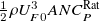 $\frac {1}{2}\rho U_{F0}^3 ANC_{P}^{\textrm {Rat}}$
, which is
$\frac {1}{2}\rho U_{F0}^3 ANC_{P}^{\textrm {Rat}}$
, which is
 $N$
times the rated turbine power (15 MW in this case) when
$N$
times the rated turbine power (15 MW in this case) when
 $U_{F0}$
is at the rated wind speed. This means that, if
$U_{F0}$
is at the rated wind speed. This means that, if
 $U_{F0}$
is always at the rated wind speed, this green line represents the scenario where the capacity factor (CF) is fixed at 100
$U_{F0}$
is always at the rated wind speed, this green line represents the scenario where the capacity factor (CF) is fixed at 100
 $\%$
. Hence, these theoretical results in Figure 8 illustrate how quickly the CF may decrease as we increase the number of turbines, especially in a small wind farm with a low ABL height (e.g. if
$\%$
. Hence, these theoretical results in Figure 8 illustrate how quickly the CF may decrease as we increase the number of turbines, especially in a small wind farm with a low ABL height (e.g. if
 $h_0=0.4$
km and
$h_0=0.4$
km and
 $U_{F0}$
is always at the rated wind speed, the maximum CF of this offshore wind farm with
$U_{F0}$
is always at the rated wind speed, the maximum CF of this offshore wind farm with
 $L=10$
km and
$L=10$
km and
 $N=200$
would be only approximately
$N=200$
would be only approximately
 $34\,\%$
, as can be seen in Figure 8a). In reality, both
$34\,\%$
, as can be seen in Figure 8a). In reality, both
 $U_{F0}$
and
$U_{F0}$
and
 $h_0$
would change with time and thus the CF would depend on their probability distributions, but the trend of the impact of
$h_0$
would change with time and thus the CF would depend on their probability distributions, but the trend of the impact of
 $L$
and
$L$
and
 $N$
on the CF would remain the same. Although not shown here for brevity, these power curves can also be predicted very quickly for different rotor design scenarios, opening the possibility of optimising rotor design and farm design in a coupled manner.
$N$
on the CF would remain the same. Although not shown here for brevity, these power curves can also be predicted very quickly for different rotor design scenarios, opening the possibility of optimising rotor design and farm design in a coupled manner.
Dependence of the non-dimensional maximum farm power
 $NC_{PG(\textrm {max})}$
on the number of turbines (IEA 15 MW,
$NC_{PG(\textrm {max})}$
on the number of turbines (IEA 15 MW,
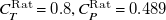 $C_T^{\rm {Rat}}=0.8, C_P^{\rm {Rat}}=0.489$
) for an offshore wind farm (
$C_T^{\rm {Rat}}=0.8, C_P^{\rm {Rat}}=0.489$
) for an offshore wind farm (
 $C_{f0}=0.002$
,
$C_{f0}=0.002$
,
 $C_\chi =0.14$
) with three different farm sizes: (a)
$C_\chi =0.14$
) with three different farm sizes: (a)
 $L=10$
km; (b)
$L=10$
km; (b)
 $L=20$
km; and (c)
$L=20$
km; and (c)
 $L=30$
km (where
$L=30$
km (where
 $S_F/A=L^2/0.04$
is assumed). Solid lines,
$S_F/A=L^2/0.04$
is assumed). Solid lines,
 $h_0=0.8$
km. Dashed lines,
$h_0=0.8$
km. Dashed lines,
 $h_0=0.6$
km. Dash-dotted lines,
$h_0=0.6$
km. Dash-dotted lines,
 $h_0=0.4$
km.
$h_0=0.4$
km.

5. Conclusions
In this study, we have extended the two-scale momentum theory for wind farm aerodynamics (Nishino & Dunstan Reference Nishino and Dunstan2020; Kirby et al. Reference Kirby, Dunstan and Nishino2023) to account for power losses due to non-ideal rotor design and turbine layout effects. Most importantly, we have introduced the turbine layout factors
 $\chi$
,
$\chi$
,
 $\chi _T$
and
$\chi _T$
and
 $\chi _P$
in (3.5), allowing us to properly differentiate the ‘internal’ power loss (due to direct turbine–wake interference, reducing the inflow speed for individual turbines relative to the farm-average wind speed) from the ‘external’ power loss (due to farm–atmosphere interaction, reducing the farm-average wind speed). We then proposed simple analytical sub-models for the rotor efficiency and the layout factors to provide a holistic view of the power performance of realistic wind farms. We also presented an iterative method based on the extended theory to quickly calculate the optimal farm induction factor that maximises the farm power for a given set of conditions, including the ABL height. Finally, we used the theory to demonstrate how the maximum power of a realistic offshore wind farm would change with the farm size and the number of turbines at different ABL heights.
$\chi _P$
in (3.5), allowing us to properly differentiate the ‘internal’ power loss (due to direct turbine–wake interference, reducing the inflow speed for individual turbines relative to the farm-average wind speed) from the ‘external’ power loss (due to farm–atmosphere interaction, reducing the farm-average wind speed). We then proposed simple analytical sub-models for the rotor efficiency and the layout factors to provide a holistic view of the power performance of realistic wind farms. We also presented an iterative method based on the extended theory to quickly calculate the optimal farm induction factor that maximises the farm power for a given set of conditions, including the ABL height. Finally, we used the theory to demonstrate how the maximum power of a realistic offshore wind farm would change with the farm size and the number of turbines at different ABL heights.
The farm power characteristics defined and predicted by the two-scale momentum theory, such as the relationship between the farm power and the farm induction factor, are as fundamentally important for wind power generation as the turbine power characteristics defined and predicted by the classical BEM theory. Just like the BEM theory forms the basis for modern wind turbine design, the two-scale momentum theory has the potential to form the basis for future wind farm design. To further validate the two-scale theory not only for idealised wind farms (as was done by Kirby et al. Reference Kirby, Nishino, Lanzilao, Dunstan and Meyers2025), but also for realistic wind farms, we would need LES of large wind farms with realistic turbine models (actuator-line models, for example) in future studies. It would also be important to further improve the accuracy and applicability of the analytical sub-models in the theory, especially those for the momentum availability factor
 $M$
, and the turbine layout factors
$M$
, and the turbine layout factors
 $\chi _T$
and
$\chi _T$
and
 $\chi _P$
. For example, an extension of the analytical
$\chi _P$
. For example, an extension of the analytical
 $M$
model has been proposed very recently by Baungaard et al. (Reference Baungaard, Nishino and Kirby2026), replacing the ABL height
$M$
model has been proposed very recently by Baungaard et al. (Reference Baungaard, Nishino and Kirby2026), replacing the ABL height
 $h_0$
in (2.10) with a ‘corrected’ ABL height to include the dependency on the ABL Rossby number.
$h_0$
in (2.10) with a ‘corrected’ ABL height to include the dependency on the ABL Rossby number.
As noted earlier in § 3.2, the turbine layout factors can also be predicted numerically, instead of analytically, using an existing engineering wake model (in a similar manner to Legris et al. (Reference Legris, Pahus, Nishino and Perez-Campos2023) and Pahus et al. (Reference Pahus, Nishino, Kirby and Vogel2024), although these earlier studies did not define the layout factors explicitly as in the present study). To better predict the layout factors numerically, however, existing wake models will need to be improved to account for, e.g. local acceleration of the flow bypassing each turbine. Such an extended wake model is currently being developed, but further studies are needed in this area. The proposed simple analytical layout factor model implicitly accounts for the effect of local flow acceleration by obtaining its empirical parameter
 $C_\chi$
from LES data for a typical range of regular turbine layouts (i.e. turbine spacing
$C_\chi$
from LES data for a typical range of regular turbine layouts (i.e. turbine spacing
 $s_x$
,
$s_x$
,
 $s_y$
and wind direction
$s_y$
and wind direction
 $\theta$
) but, due to the scarcity of available LES data for finite-size farms with different wind directions, we used LES data for infinitely large wind farms in this study. Although the layout factors and the parameter
$\theta$
) but, due to the scarcity of available LES data for finite-size farms with different wind directions, we used LES data for infinitely large wind farms in this study. Although the layout factors and the parameter
 $C_\chi$
are expected to be insensitive to the wind farm size, it would be better to use finite-size wind farm LES data (when available) to fully confirm this in future studies.
$C_\chi$
are expected to be insensitive to the wind farm size, it would be better to use finite-size wind farm LES data (when available) to fully confirm this in future studies.
Acknowledgements
The authors thank Dr Andrew Kirby for providing his LES data from Kirby et al. (Reference Kirby, Nishino and Dunstan2022), which were used by T.N. to create Figure 2. The authors also thank Dr Mads Baungaard for proofreading the original manuscript.
Data availability statement
A set of Matlab codes for the iterative method described in § 4.2 is available at https://github.com/asm-smyth/windFarmModelling-twoScaleMomentum-1. The data required to create Figure 2 are available at https://github.com/AndrewKirby2/wind-farm-modelling.
Author contributions
T.N. proposed the power loss mechanisms in § 3.1 and the rotor efficiency model in § 3.3. T.N. and A.S.M.S. jointly developed the layout factor model in § 3.2. A.S.M.S. derived the iterative method in § 4.2.
Funding statement
This research has been partially supported by the UK Met Office (WCSSP programme, SA24-2.4) and the UK Natural Environment Research Council (NERC ECOFlow programme, NE/Z504099/1).
Competing interests
The authors declare no conflict of interest.
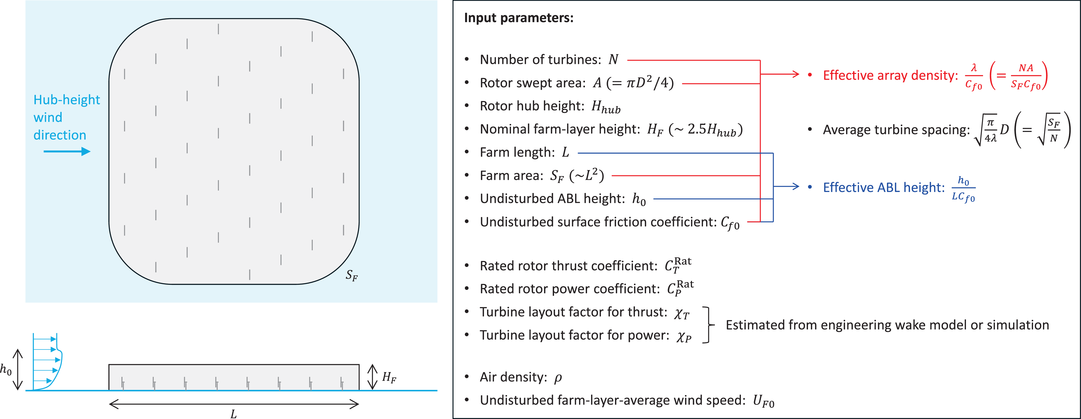


 Open access