Introduction

Ice divides are places on ice sheets where the ice-velocity and heat-flow patterns are distinctive and unique because of the non-linear nature of the constitutive relation for ice. The low deviatoric-stress state at an ice divide causes deep ice to be stiff to deformation directly beneath the divide (Reference RaymondRaymond, 1983). In addition, special accumulation patterns at ice divides such as wind scouring (Reference Fisher, Koerner, Paterson, Dansgaard, Gundestrup and ReehFisher and others, 1983) can alter the flow field. Altered ice flow also affects the temperature field. These patterns in ice and heat flow cause isochrones and isotherms to be arched in a zone a few ice thicknesses wide beneath a steady ice divide. The shapes of isochrones and isotherms are also sensitive to the history of the divide position. Under steady flow conditions with no motion of the divide, the predicted arch size for isochrones and isotherms is large. With relatively slow movement of the divide, the arch is more subdued, while with rapid divide motion the arch can be undetectable. The present shape of isochrones and isotherms at a divide may record past positions of the divide and provide clues to past geometry of the ice sheet. The memory time depends on the dynamic and thermal characteristics of the ice sheet and is not necessarily the same for isochrones and isotherms.

Arched isochrones have been observed with ice-penetrating radar beneath several ice divides in West Antarctica. Their shapes have been used to infer past motion of the divide, relative changes at the boundaries of the ice sheet, spatial accumulation variability, recent ice-sheet thinning rates, and timing of ice-sheet formation (Reference Nereson, Raymond, Waddington and JacobelNereson and others, 1998; Reference Conway, Hall, Denton, Gades and WaddingtonConway and others, 1999; Reference Vaughan, Corr, Doake and WaddingtonVaughan and others, 1999; Reference Nereson and RaymondNereson and Raymond, 2001). While each of these interpretations is relevant to a specific site, we present here the generic patterns of isotherms and isochrones associated with moving ice divides. We develop a generic kinematic flow model by abstracting only the features necessary to deform isochrones and isotherms. We calculate characteristic time and length scales governing the memory time and resolution of past changes in divide position that can be inferred from isochrones and isotherms.

Our aim is to provide the theoretical framework in which field measurements of isochrones and isotherms are used to infer the divide-position history for an ice sheet. In theory, isochrones are identified by contouring the age field, and isotherms are identified by contouring the temperature field. In practice, isochrone shapes are typically identified directly using radar measurements without knowledge of the age field, while isotherms are typically identified by temperature measurements at various locations in a borehole or set of boreholes. To be consistent with typical field measurements, we describe the shape of a given isochrone in terms of a height (not age) difference Δz(x, z), relative to the far-field layer height z; and we describe the shape of a given isotherm in terms of a temperature difference ΔT(x, z) relative to the far-field ice-sheet temperature at a given depth.

Ice-Flow Model

To calculate isochrone shapes in a migrating flow field, we track ice particles in a continuous two-dimensional kinematic flow field in which the velocities at the ice surface are determined by mass continuity (vertical velocity = accumulation rate at the surface), and velocities at depth follow prescribed shape functions which can vary with position. Tildes indicate dimensional quantities. We consider two mechanisms for the formation of a divide arch in the isochrones: (1) a non-linear constitutive relation (strain-rate-dependent viscosity) and (2) local accumulation scouring (associated with the topography of a divide). For the first case, the depth variation of the horizontal and vertical velocity field varies with position and is described by a partitioning between shape functions typical of flow remote from the divide (flank) and shape functions typical of flow at the divide for ice deforming according to Glen’s flow law where the strain rate is proportional to the third power (n = 3) of the shear stress. For the second case, the velocities are scaled to the accumulation rate at the ice surface, and the shape of the depth variation of flow does not vary with . Our formulation is similar to that of Reference ReehReeh (1988) and Reference Nereson, Raymond, Waddington and JacobelNereson and others (1998). We choose to use a kinematic flow model over other methods such as a stress-balance model (e.g. Reference RaymondRaymond, 1983; Reference HvidbergHvidberg, 1996) because this allows us to capture the essential causes and effects of layer shape changes and to easily prescribe and control the rate of divide motion, while keeping the problem as simple as possible. Our kinematic model accurately reproduces isochrone shapes predicted from a full stress-balance model for a steady-state ice divide. Divide motion is simulated by moving the flow field laterally at a constant rate as the ice particles are tracked. Isochrone shapes are calculated by joining particle tracks at constant ages.

Shape-function description of ice velocities

Consider a steady-state ice sheet deforming in plane strain with no divide motion. Let denote distance along flow from the divide and denote distance upward from the bed. We assume flat bedrock and uniform ice thickness independent of . This assumption is justified for a kinematic model because ice-thickness variations are small near an ice divide and because flow in our model can be determined by continuity, rather than by stress balance. Distance coordinates are scaled to the ice thickness , so that the non-dimensional position is , and . Horizontal and vertical velocities and the accumulation pattern are scaled to a reference accumulation rate so that , , and .

For a given accumulation pattern b(x), the horizontal velocity averaged over depth (as indicated by an overbar) is determined by continuity:

(1)

The depth variation of horizontal velocity at a given scaled distance x from the divide is represented by a shape function ϕ(x, z) that varies with x and z so that

(2)

The shape function must satisfy ϕ(x, 0) = 0 (frozen bed) and so that where u _s is the non-dimensional horizontal velocity at the ice surface.

The vertical velocity field w(x, z) is determined from incompressibility ∂ _xu = −∂ _zw. Differentiation of u(x, z) with respect to x and integration with respect to z yields the vertical velocity field:

(3)

When z = 1, w(x, 1) = b(x). To simulate a moving divide, we move the velocity field at a rate and make calculations in a reference frame (indicated by “*”) that moves with the divide. The horizontal velocity in the moving-divide reference frame is

(4)

and the vertical velocity in the moving reference frame is unchanged so that w*(x*, z*) = w(x*, z*). With this construction, x = 0 is always the divide position. We drop the asterisks from now on and assume that we are always in the moving-divide reference frame.

Divide flow from non-linear constitutive law

Assuming that the arched internal layers beneath the divide are caused solely by non-linearity of the stress–strain-rate relation for ice, and the accumulation rate b(x) = 1 is uniform, we prescribe the horizontal velocity shape function ϕ(x, z) in Equation (2) as a linear combination of a shape function ϕ _d(z) for pure divide flow with a non-linear flow law, and a shape function ϕ _f(z) for pure flank flow,

(5)

The function α(x) describes the partitioning between flank-like and divide-like flow regimes. The partitioning function α(x) should decrease monotonically from unity at the divide to zero far from the divide. Substitution of Equation (5) into the vertical velocity Equation (3) yields

(6)

The integrals and are shape functions for the divide and flank vertical velocities. The vertical velocity at position x is partitioned between ϕ _d and ϕ _f according to the function

(7)

and the total velocity field can be written as:

(8)

The horizontal and vertical velocities have different partitioning functions which are related via continuity requirements according to Equation (7). Once we choose shape functions ϕ _d(z) and ϕ _f(z) (or ψ _d(z) and ψ _f(z)) and a partitioning function α(x) (or β(x)) for either horizontal or vertical velocity, the other velocity equation directly follows. Reference Nereson, Raymond, Waddington and JacobelNereson and others (1998) took a slightly different approach and used only one partitioning function for u(x, z). Vertical velocity w was then determined directly from continuity. Our present approach results in simpler and more intuitive expressions for the velocity field.

We use a Dansgaard–Johnsen formulation for the velocity shape functions (Reference Dansgaard and JohnsenDansgaard and Johnsen, 1969). This allows a wide variety of velocity shapes to be represented while maintaining analytical simplicity. The flank horizontal velocity shape function ϕ _f is given by:

(9)

and ϕ _d(z) is defined by a similar equation with an associated h _d value such that 0 < h _f < h _d < 1. The corresponding vertical velocity shape function is:

(10)

and an associated equation for ϕ _d(z) given h _d.

Our choice for h _d and h _f determines the difference between flank and divide velocities (and hence arch amplitude), which depends on degree of non-linearity n in the ice-flow law . When n = 1, h _d = h _f, and an arch does not form. When n = ∞ (perfectly plastic ice), ice beneath the divide is infinitely stiff to deformation (w (0, z) = 0) and the amplitude of the arch is equal to the ice thickness. 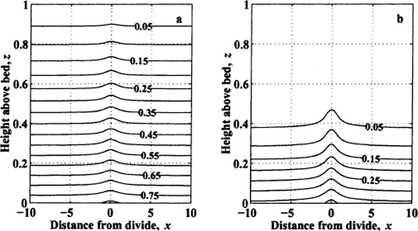The parameters h _f = 0.2 and h _d = 0.6 are chosen so that the velocity profiles and associated age-depth relationships both at the divide and remote from the divide match (within 5%) those predicted by a full stress-balance calculation of ice flow where the degree of non-linearity is given by n = 3 (Reference RaymondRaymond, 1983; Reference Nereson, Waddington, Raymond and JacobsonNereson and others, 1996). Figure 1 shows the vertical velocity profiles for pure flank (α = β = 0; solid line) and pure divide (α = β = 1; dash-dotted line) conditions.

Fig. 1.

Depth profiles of vertical velocity w for pure flank (β = 0, solid curve) and pure divide (β = 1) flow conditions. The divide-flow regime is caused by either a non-linear flow law (dot-dashed line) or local accumulation scouring that moves with the divide (dashed curve).

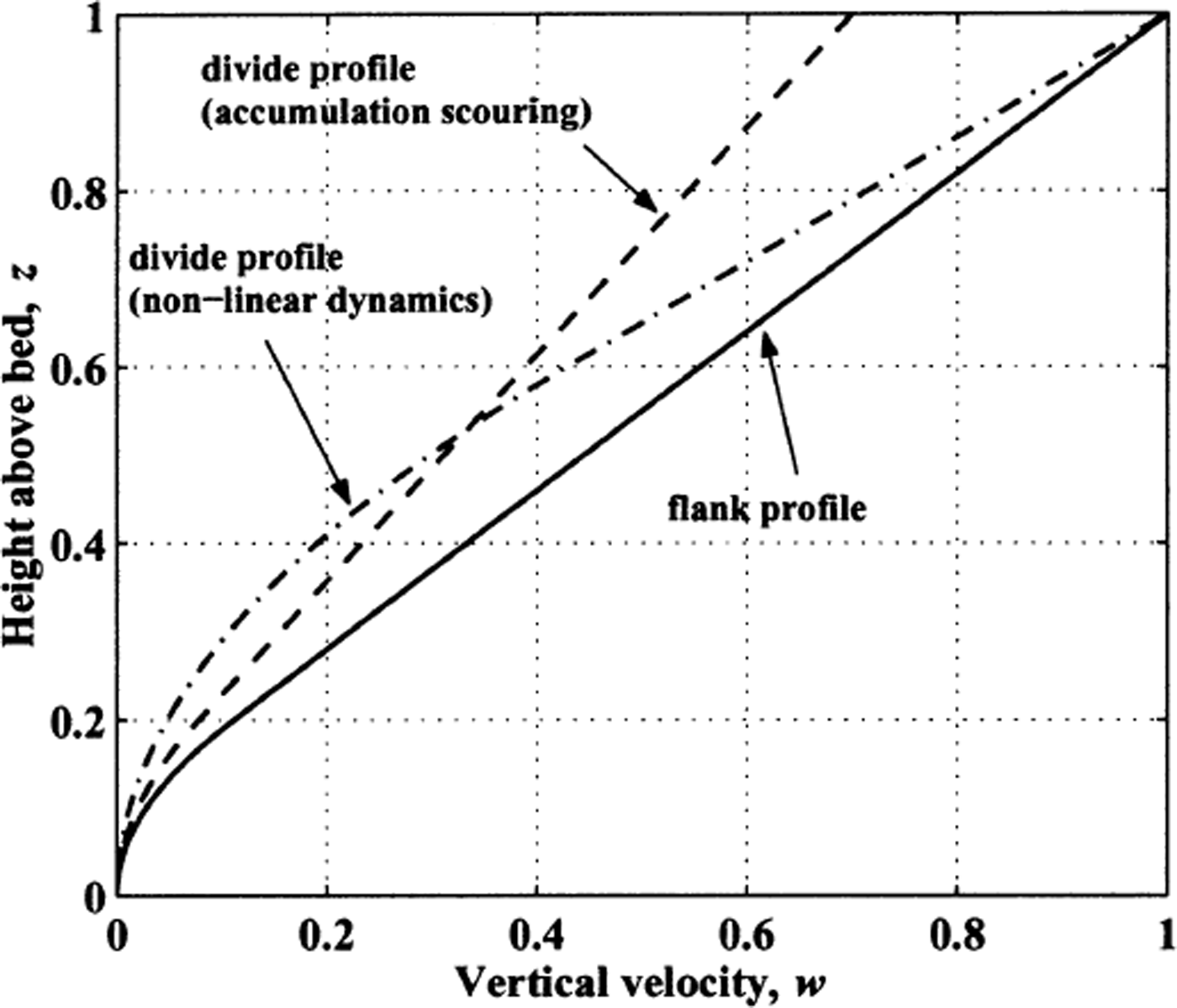
Figure 2 shows the partitioning function pair α(x) (solid dots) and β(x) (open circles) from a stress-balance model of ice flow where the degree of non-linearity is given by n = 3 (Reference RaymondRaymond, 1983; Nereseon and others, 1996). The divide influence on horizontal velocity extends several ice thicknesses out from the divide. For vertical ice motion, however, the divide influence is confined to within about 1 ice thickness of the divide. This difference between horizontal and vertical partitioning of flank and divide flow is evident in the stress-balance models by Reference RaymondRaymond (1983) and Reference HvidbergHvidberg (1996).

Fig. 2.

Partitioning functions α(x) (Equation (12), solid curve) and β(x) (Equation (11), dashed curve) for σ = 0.5. Solid dots and open circles correspond to partitioning between flank and divide flow from analysis of horizontal (solid) and vertical (open) velocity profiles from a finite-element stress-balance calculation.

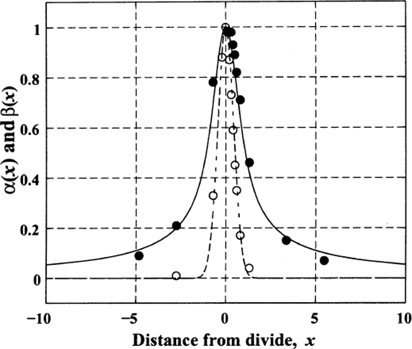
For modeling purposes, we define analytical, continuously differentiable partitioning function pairs that match the stress-balance model (within 5%), have a value of 1 at the limit as x → 0, monotonically approach 0 far away from the divide, and obey Equation (7). We choose β(x) to be a Gaussian function where the divide zone is defined by the characteristic width σ:

(11)

The positions x = ±σ mark the inflection points of the function β, and σ is roughly equivalent to the half-width of β(x) at half its maximum value. Equation (7) requires

(12)

The value σ ≈ 0.5 gives the best match in a least-squares sense to the stress-balance model velocities in Figure 2. The resultant total width of the divide zone of about 1 ice thickness is consistent with an estimate based on the transition from pure shear to simple shear-type deformation in Reference RaymondRaymond (1983).

We use velocity Equations (8) and (4), together with the partitioning functions (11) and (12) and prescribed values for h _d and h _f to track ice particles in a migrating flow field. We assume uniform accumulation, so that b(x) = 1.

Divide signature from local accumulation minimum

The traditional non-linear theory for ice deformation may break down at some ice divides because of the low-stress regime there (Reference Waddington, Raymond, Morse and HarrisonWaddington and others, 1996). If ice behaves predominantly as a linear fluid in the divide zone, then an arch would not be expected to form in the internal layers. However, a local low in the accumulation pattern over an ice divide caused by wind scouring (Reference Fisher, Koerner, Paterson, Dansgaard, Gundestrup and ReehFisher and others, 1983) could also leave an arched internal layer pattern.

To simulate this condition, we remove the influence of a non-linear flow law by specifying velocity shape functions ϕ and ψ that do not vary with position x so that ϕ(x, z) = ϕ _f(z) and ψ(x, z) = ψ _f(z). However, we prescribe an accumulation pattern b(x) that includes a local minimum over the divide. We represent the accumulation low as one cycle of a cosine bell curve where W defines the width of the divide zone (in units of ) and Δb defines the scouring rate (in units of the far-field accumulation rate ):

(13)

We expect that W ≈ 1 since our accumulation minimum is associated with local scouring at the divide and the topography of ice divides becomes rounded about 1 ice thickness from the divide (Reference Scambos, Nereson and FahnestockScambos and others, 1998). We take W = 1 for the remaining analysis in this paper. Since the velocity shape function does not vary in x, the velocity equations reduce to the familiar Dansgaard–Johnsen formulation (Reference Dansgaard and JohnsenDansgaard and Johnsen, 1969):

(14)

and

(15)

Figure 1 shows the depth variation of vertical velocity for pure flank (solid curve) and pure divide flow (dashed curve).

Given accumulation scouring parameters W and Δb (Equation (13)), we simulate divide motion according to Equation (4) by moving the flow field defined by Equations (14) and (15) at a constant rate m. For these calculations we set W = 1, Δb = 0.3 and h _f = 0.2.

Model Results: Isochrones

In reality, most ice divides probably have signatures from both non-linear rheological properties and a local accumulation minimum. Both processes may need to be considered when interpreting internal layering beneath specific ice divides (Reference Nereson, Raymond, Waddington and JacobelNereson and others, 1998). However, here we consider only the two end-members.

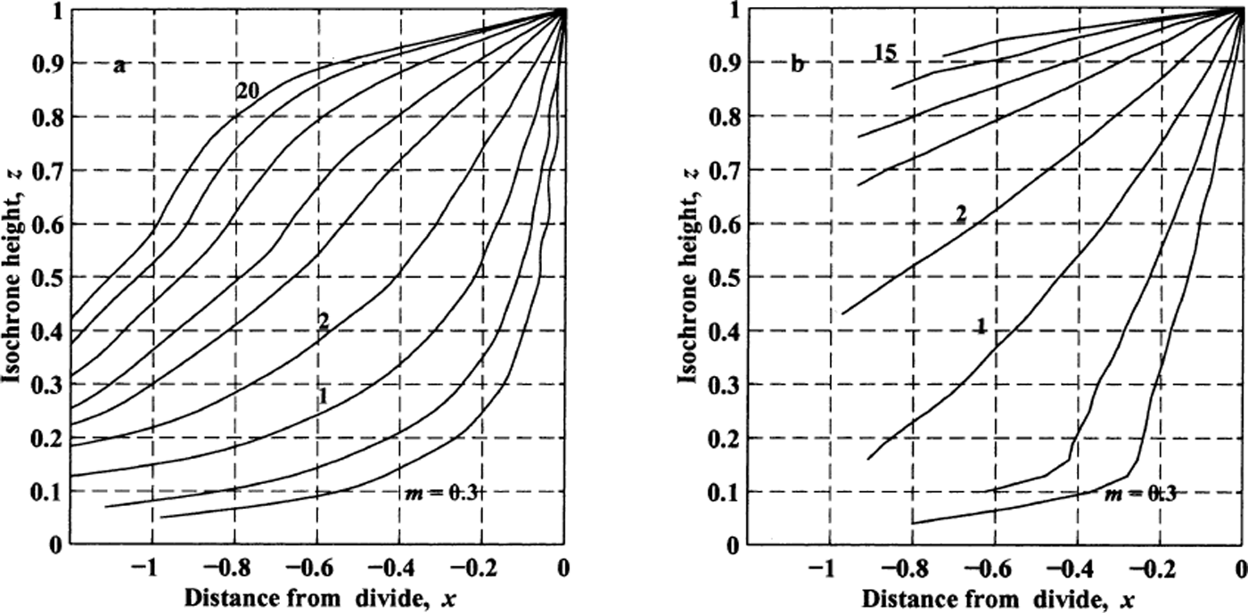
Figure 3 shows the predicted isochrone shapes for various rates of divide migration, m, for each mechanism of layer arch formation. Qualitatively, the arch shape is similar in both cases. We define the amplitude of the arch Δz as the difference between the maximum height of a given isochrone (near the divide) and its far-field height remote from the divide. With no divide motion, the divide arch is pronounced and symmetric, and reaches a maximum amplitude that depends either on the non-linearity of the ice constitutive relation (e.g., when n = 3, maximum Δz ≈ 0.10) or on the degree of accumulation scouring (e.g., when Δb = 0.3, maximum Δz ≈ 0.12). With increasing divide-motion rates, the amplitude of the divide arch is more subdued and the shape is more asymmetric.

Fig. 3.

Isochrone pattern caused by (a–d) non-linear flow law (n = 3) and by (e–h) local accumulation minimum (30%) over divide (W = 1, Δb = 0.3) for various divide-migration rates m. The divide is at x = 0 and moving to the right.

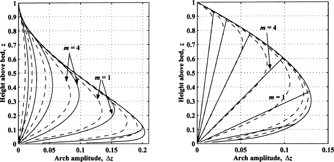
Figure 4 shows how the amplitude Δz of the arch varies with the far-field layer height z for increasing migration rate m and for each mechanism of divide flow. Since the layers must conform to the surface and the bed, the largest arch occurs at a depth some distance above the bed. The amplitude of the arch is large when m ≤ 1, is reduced to half of its original amplitude when m = 2, and is nearly gone when m > 10.

Fig. 4.

Divide arch amplitude vs height above the bed on flanks for (a) non-linear constitutive relation (n = 3) and (b) local accumulation minimum (Δb = 0.3) at various migration rates: m = [0, 0.3, 0.5, 1, 2, 4, 6, 10, 15, 20]. In both cases, when m = 2, the maximum arch amplitude is approximately half of the value at m = 0 (no divide migration).

The depth profile of the arch amplitude is different for each of the two divide-flow mechanisms. The maximum arch amplitude occurs at shallower depths in the accumulation scouring case. Further experiments (not shown) indicate that this is true regardless of choice of scouring parameters Δb and W. At high migration rates, the maximum arch amplitude is found very near the surface. Also, the amplitude of the arch caused by the accumulation low has a linear variation with depth near the ice surface, while the arch caused by a non-linear constitutive relation has a quadratic variation with depth. This difference is related to the depth variation of vertical velocity w(z) for each mechanism. With a non-linear flow law, the difference between the vertical velocity profiles for divide and flank flow is most pronounced at depth, while for accumulation scouring it is most pronounced at the surface (Fig. 1).Reference Vaughan, Corr, Doake and WaddingtonVaughan and others (1999) used this near-surface difference to determine which process caused internal layer arching at several sites on Fletcher Promontory, West Antarctica.

The location of the shallowest point on each isochrone (which we will call the apex) is related to the divide-motion rate. Without divide motion, the apex of each layer is directly under the divide. With increasing divide motion, the apex is increasingly offset from the modern divide location, and the magnitude of the offset increases with depth. For isochrones detected with radio-echo sounding techniques at ice divides, this simple measure can be used as a quick estimate of direction and relative rate of divide motion (Reference Nereson, Raymond, Waddington and JacobelNereson and others, 1998). Figure 5 shows how the position of the apex varies with depth and with migration rate for each divide-flow mechanism. For m < 4, the apex-position curve has a positive curvature and a slope greater than unity near the divide, while for m > 4, the trend has a negative curvature and a slope less than 1 near the divide. In general, the arch offset at depth for a given migration rate is less for a non-linear flow law than for accumulation scouring.

Fig. 5.

Position of arch apex vs height above the bed for various migration rates: m = [0, 0.3, 0.5, 1, 2, 4, 6, 10, 15, 20]. (a) Non-linear ice-flow law, n = 3. (b) Local accumulation minimum, W = 1, Δb = 0.3.

An Analytical Approach: Isochrones

A simple analytical description of the problem would show which features of the numerical solution are fundamental and robust. In addition, analytical tools would allow simple interpretation of isochrone arch amplitude and position in terms of migration rate, without numerical models. We propose that only a few free parameters are necessary to capture the essential features of isochrone shape, and that this shape can be described analytically. These fundamental parameters are ice thickness , accumulation rate , divide-motion rate , and scalars defining the velocity field (e.g. h _f and h _d).

Layer shapes

The asymmetry of the layer shapes in Figure 3 can be explained by a simple conceptual model of divide migration. Consider an Eulerian view where we are interested in the ice-deformation process at a particular position (x, z) in the ice column. We imagine a migrating divide zone as a “boxcar” function that passes by our position on the ice sheet. Divide flow is “on” during the time the divide zone passes our position and “off” otherwise. We assume that ice moves only downward, and we ignore complications such as smooth partitioning (Equation (5)) between flank-and divide-flow regimes, and the extending component of flow away from the divide.

We define a characteristic time associated with the time a given column of ice spends in the divide zone as the divide passes by at a rate :

(16)

where is the characteristic time for vertical ice flow and is the non-dimensional migration rate. Since we take W = 1 for accumulation scouring, is the same for both divide-flow mechanisms. When m = 1, the characteristic time for horizontal divide motion is the same as the characteristic time for vertical ice flow . For m ≪ 1, vertical ice flow dominates the development of isochrone shapes, and horizontal divide motion has a minimal effect. The time a given column of ice spends in the divide zone is greater than the age of the ice in most of the ice column, and most layers in the column have enough time to develop a steady-state arch. Since divide flow is “on” uniformly inside the divide zone, each layer develops a “boxcar”-like arch.

For increasing m, horizontal divide motion inhibits the development of the isochrone arch. Most of the ice in the ice column passes through the divide zone before the layers can fully develop an arch. In addition, the arch becomes more asymmetric. Ice at the leading edge of the divide zone is just leaving the flank zone and encountering divide flow for the first time; it has had no time to develop an arch. Ice at the trailing edge of the divide zone may have experienced divide flow for most or all of its history, so layers there have a well-developed arch. Ice behind the moving divide has some memory of previously being in the divide zone, so the isochrones there are still somewhat elevated. Because information about the past divide position is lost after the migrating divide zone passes over a column of ice, is also a memory time, marking how long isochrones can maintain a record of divide position (given a migration rate m).

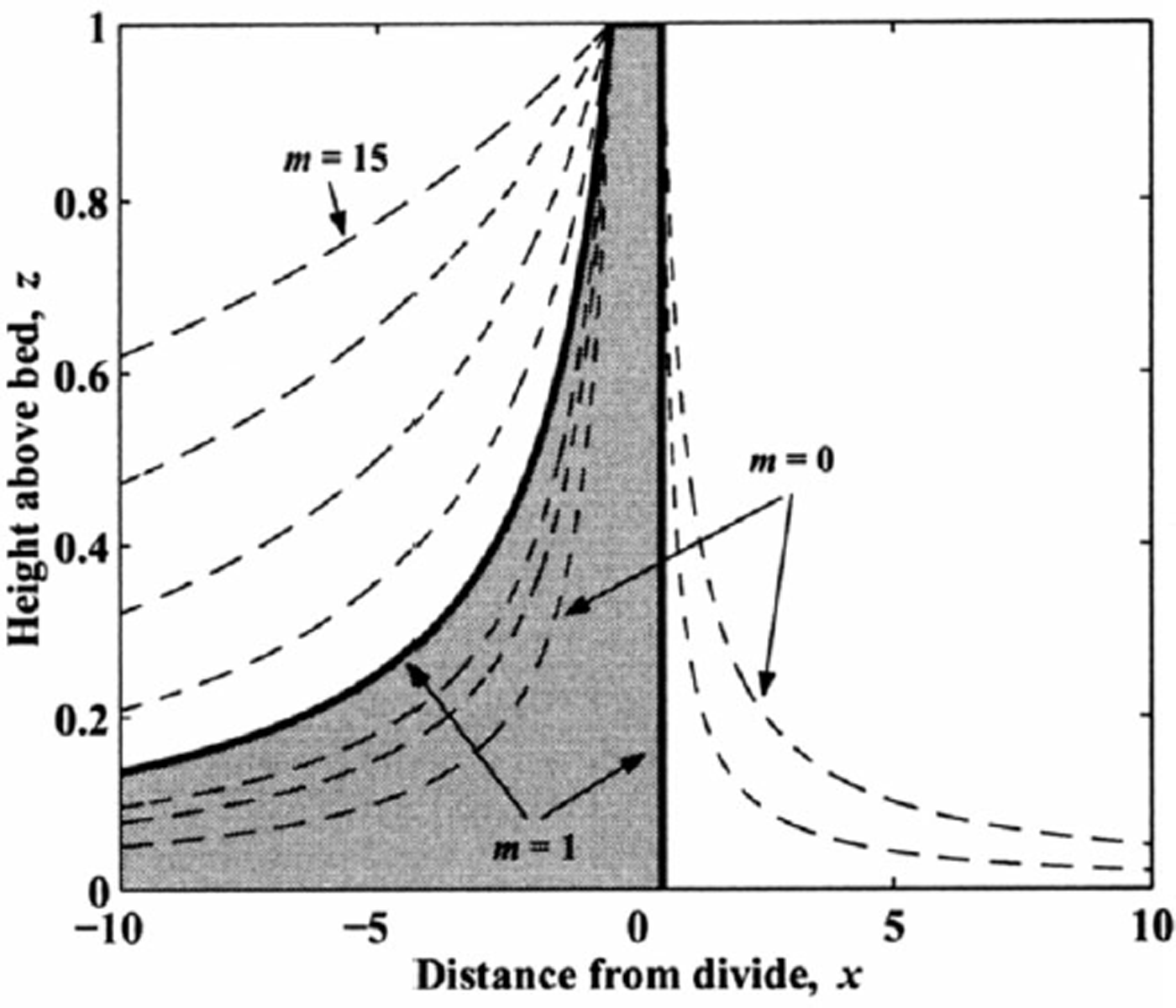
Although we neglect horizontal ice flow in our conceptual model, horizontal flow extends the influence of the divide by carrying arched layers out of the divide zone. With divide motion, this influence is asymmetric. In our analytical model where the divide zone has a distinct edge, flowlines originating at the edges (x ≈ ± 0.5) mark the boundary between ice that has experienced divide flow and ice that has not. Using a simple flank-flow vertical velocity (h _f = 0), and now incorporating the extending horizontal flow (previously neglected), the flowlines originating at the edges of the divide zone are

(17)

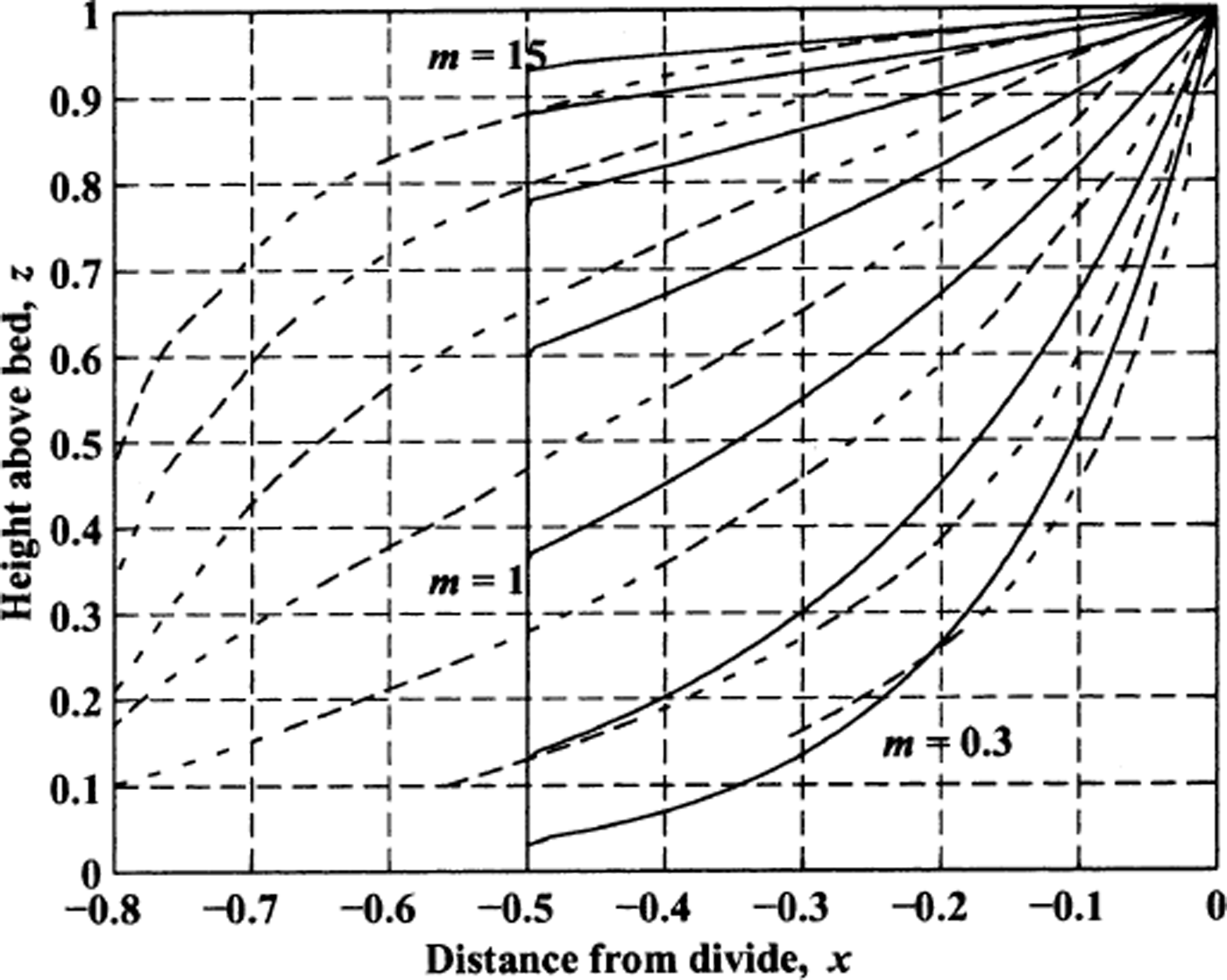
for positive and negative values of x, respectively. The region of divide influence, defined by Equation (17), is shown in Figure 6 for various values of m. When m > 0.5, the scaled half-width of the divide zone, a vertical boundary develops ahead of the moving divide front so that no ice ahead of the divide has experienced divide flow. In the lee of the moving divide, its influence is felt at large distances away from the divide when m > 1. More generally, for h _f > 0, Equation (17) determines the divide influence boundary in the upper part of the ice sheet (z > h _f) where the vertical strain rate is constant. This asymmetric influence pattern also contributes to the asymmetric layer shapes in Figure 3. When the velocity in the divide zone is controlled by continuous partitioning functions (Fig. 2), the divide-zone edge is less distinct, but Equation (17) still approximates the zone of divide influence.

Fig. 6.

Boundaries of divide-flow influence for various migration rates (m = [0, 0.3, 0.5, 1, 2, 4, 8, 15]). The gray shaded region shows the area of divide influence for m = 1. Below the boundary, ice has experienced some divide flow and isochrones are arched. Above the boundary, ice has experienced pure flank flow. For m ≥ 0.5, the upstream influence of the divide zone is restricted to x ≤ 0.5 because no ice escapes the front of the moving divide zone.

Arch amplitude

For a steady-state divide, the arch amplitude Δz _steady is simply the difference between heights (z _f and z _d) for a given layer of age a when comparing flank and divide depth–age relationships. This can be found by integrating the vertical velocity profiles w _f(z) and W _d(z). For a new divide, where divide flow is imposed at time t = 0 on a set of initially flat flank layers, the total evolution time for arch growth at a given depth is equal to the age of ice at that depth. The layer that was at the surface at the moment of divide onset separates layers below, which experienced the prior flow pattern, from those above, which have no memory of the prior flow pattern. When this layer reaches any depth, the arch at that depth has evolved to its final steady-state value. Conversely, the time for total decay of the arch (Δz = 0) at a given depth after the divide moves away is also equal to the age of the flank ice at that depth. The transitional layer is the ice deposited at the surface at the moment that the divide left. When this layer reaches any depth, then the arch is entirely gone at that depth.

This analysis can be applied to the case where the migrating divide zone is simplified as a moving “boxcar” function of width W = 1 that passes over each column of ice at rate . Let t = 0 denote the time when the moving divide zone encounters a particular ice column. The time that this column of ice spends in the divide zone is . In scaled units, . During this time (t ≤ τ _m), a divide arch can grow in the ice column. At shallow depths, where scaled age of the flank ice is less than τ _m, ice in the column has experienced only divide flow since its deposition, and the arch is fully developed. At greater depths, where the age of the ice is greater than τ _m, ice in the column has experienced a combination of first flank then divide flow, and arch growth terminates prematurely at t = τ _m before reaching full steady-state amplitude. At times t > τ _m, after the divide has passed by our ice column, the divide arch decays from either its steady-state value or its truncated value.

To arrive at expressions for the development of the divide arch amplitude, Δz, for a given migration rate m, we apply these concepts to a series of adjacent ice columns for the specific cases where divide flow is due to a non-linear flow law or to a local minimum in the accumulation pattern.

Non-linear flow law

A simple way to represent a non-linear constitutive relation is to use the end-member velocities where h _f = 0 (“Nye flow” (Reference NyeNye, 1963)) and h _d = 1 (“Raymond flow” (Reference RaymondRaymond, 1983)). Then for flank flow and for divide flow. These arches are larger than those found with a more realistic vertical velocity pattern, but have the advantage of being analytical. The steady-state arch amplitude Δz _steady (a) for a layer with age a is then the difference in layer height between the divide and flank:

(18)

The variation of arch amplitude Δz(z) with height above the bed is found by substituting the age–depth relation for flank ice, z _f(a) = exp (−a). This fully developed arch is found at shallow depths where time t since divide arrival is greater than the age a of the layer.

Straightforward analysis (unpublished) shows that the divide arch growth at a given depth z in time t since divide onset for a set of initially flat layers is

(19)

and the decay of a steady-state arch in time t after the divide moves elsewhere is

(20)

For a divide moving at rate m (and associated total time τ _m = 1/m that a given column of ice is in the divide zone), the arch amplitude for a layer at height z on the flank that has experienced divide flow since its deposition (z > exp(−1/m)) is found by substituting the age of the flank ice a = ln(1/z) for t in Equation (19). For older, deeper ice at z ≤ exp(−1/m) that experienced flank flow prior to t = 0, the arch amplitude is found by substituting t = τ _m = 1/m in Equation (19) so that

(21)

Figure 7a shows Δz(z) profiles from Equation (21) for various values of m. Also shown for comparison are the arch amplitudes calculated from the numerical model with h _f = 0 and h _d = 1. Our analytical expression predicts all the qualitative features of the full numerical result, and, given the additional assumptions, predicts the magnitude acceptably well. Our slight over-prediction arises because we neglect extending ice flow and we apply the divide vertical velocity over the full width of the divide zone.

Fig. 7.

Analytical estimate of the arch amplitude (solid lines) for m = [0.3,0.5, 1, 2, 4, 8, 15]. Results from the corresponding numerical model shown as dashed lines, (a) Non-linear constitutive law (Equation (21)) with h _d = 1 and h _f = 0. (b) Local accumulation minimum, Δ _b = 0.3 (Equation (25)).

Local accumulation minimum

Again assuming the Nye end-member velocity field where h _f = 0, we can obtain a comparable expression for the arch amplitude Δz(z), given a migration rate m for divide flow caused by a local accumulation minimum. Vertical velocities are W _f = −z and W _d = − z(1 − Δb). As before, the steady-state arch amplitude is the difference in heights at a given age a:

(22)

A series expansion of the exponentials in Equation (22) shows that the steady-state arch amplitude is proportional to Δb for small Δb.

For divide onset at t = 0 in initially flat layers, it is straightforward to show that the arch amplitude in the layer at depth z on the flank at time t grows according to

(23)

Similarly, the decay of a steady-state arch after the divide moves away (when t ≥ τ _m) can be shown (unpublished analysis) to follow

(24)

In the Eulerian view of the “boxcar” divide zone passing over a column of ice at a rate m, the divide arch at height z grows according to Equation (22) until the ice that was at the surface at divide onset (t = 0) reaches z. If the divide zone passes by before this ice reaches z, then the arch growth (Equation (23)) terminates at t = τ _m = 1/m. The arch amplitude in a layer at flank depth z is

(25)

Figure 7b shows the amplitude Δz(z) of the arch for various values of m (and associated τ _m) according to Equation (22) and the prediction from the full numerical model for Δb = 0.3. Our analytical approximation, which is based only on the differing vertical velocities between divide and flank flow, is similar to the full numerical calculation for a wide range of m values, demonstrating that we have captured the essential processes.

Apex position

Another useful quantity that characterizes the shape of isochrones under a migrating divide is the position of the arch apex (Fig. 5). To locate the apex, it is necessary to describe how isochrone shape varies with position x. If the divide is not moving, all ice in the divide zone experiences divide flow and a “boxcar” layer shape develops in our analytical model. The amplitude of this “boxcar” is given by the steady-state amplitude at each depth (Equation (21) or (25)). The “apex” of the layer in this case is the center of the “boxcar”. If the divide is moving, the isochrone shapes can be obtained from the equations for arch growth and decay using the transformation to the Lagrangian reference frame:

(26)

where 1/2 is the scaled half-width of the divide zone. Divide motion to the right implies time progression (since divide onset) to the left along the negative x axis. In the Eulerian reference frame, Equation (26) places the first contact with the divide zone at x = 1/2 when t = 0. Using the transformation (26), Δz(t, z) becomes Δz(x, z) in Equations (19), (20), (23) and (24), which then describe the shape of the layers, rather than their evolution at a fixed point.

When the divide is moving, not all ice in the divide zone has experienced divide-flow conditions for a sufficient amount of time to develop a steady-state arch. Ice deposited at the surface at the leading edge of the divide zone (x = 0.5 or W/2) travels downward according to the appropriate age–depth relationship for flow in the divide zone as the divide moves by at speed m. Using Equation (26), the path of this ice particle in a Lagrangian reference frame moving with the divide is

(27)

For any position x in the divide zone, Equation (27) marks a transition between (a) shallower ice that has experienced divide-flow conditions since its surface deposition so that layers have a steady-state arch, and (b) deeper ice that has experienced first flank then divide flow so that layers have not developed a steady-state arch. The path leaves the divide zone at x = −1/2 where z _trans = m/(m+ 1) (non-linear flow) or z _trans = exp[−(1−Δb)/m] (accumulation low). Since z _trans rises for increasing migration rates, the amount of ice in the divide zone above the transition path (where a steady-state arch exists) becomes smaller.

For ice in the divide zone above the transition height z _trans, the arch for a given layer has a flat section at the steady-state arch amplitude (Equation (21) or (25)).We take the apex of the layer to be the midpoint of that flat section. This position is halfway between the transition path (Equation (27)) and the trailing edge of the divide zone:

(28)

Solid curves in Figure 8 show the position of the apex for various migration rates m for non-linear ice flow in the divide zone. Dashed curves show results from the corresponding numerical model with h _f = 0 and h _d = 1. The agreement, with concave upward curvature for low m values, suggests that both approaches capture the essential controls on layer shape.

Fig. 8.

Solid curves show analytical estimate of position of arch apex for non-linear flow law (Equation (28), solid lines) for m = [0.3, 0.5, 1, 2, 4, 8, 15]. All analytical curves descend to bed at trailing edge of divide zone. Corresponding numerical model results shown by dashed lines.

For steady migration rates, the apex must occur in the divide zone. For a given layer, the portion that has experienced the most divide flow (and is therefore the apex of the divide arch) is either in the divide zone or at the trailing edge of the divide zone. Portions of the same layer behind the divide zone have experienced flank flow subsequent to divide flow, and thus are deeper than portions still in the divide zone. The apex position for the numerical model (dashed lines in Fig. 8) can exist farther from the divide because the divide zone for a non-linear flow law is defined by β(x) (Fig. 2) which has smooth tails that extend the influence of divide flow to more than 1 ice thickness from the divide.

Heat-Flow Model

Ice temperature tends to be warmer at a given depth in the divide zone compared to the flanks because of the decreased downward advection of cold ice at the divide. Therefore, isotherms, horizons of constant temperature, are also arched up ward in this zone (Reference Paterson and WaddingtonPaterson and Waddington, 1986; Reference HvidbergHvidberg, 1996). This “hot spot” beneath the divide can also influence the temperature distribution in the rock below (Reference WaddingtonWaddington, 1987). Different divide-motion rates create different isotherm shapes. Isotherms therefore contain an additional record of divide-motion history.

Just as for isochrones, the isotherm pattern under a migrating divide can be found by solving a steady-state problem because (a) we assume the divide is migrating at constant rate m, and (b) we make calculations in a reference frame that moves with the divide so that x = 0 is always the divide position. To predict the shape of these isotherms in the ice and bed when the divide is migrating, we solve the steady-state two-dimensional heat-flow equation for a ridge of uniform ice thickness, underlain by flat conductive bedrock:

(29)

where is temperature, and the two-dimensional ice-velocity field is specified. We neglect strain heating. Values for thermal conductivity k, specific heat c, density ρ and thermal diffusivity κ = k/(ρc) for rock and ice are specified in Table 1.

Table 1.

Property values used for ice and rock in the heat-flow model

Using characteristic values for velocity, time, temperature, density, heat capacity and conductivity (Table 2), Equation (29) can be written in non-dimensional form as

(30)

where K, T, R and C are non-dimensional values for conductivity, temperature, density and specific heat. In the ice, R = C = K = 1. The non-dimensional ice velocity field u is given by Equations (4) and (8). The Péclet number Pe, defined by the characteristic thermal and geometric values of the problem, can be written as the ratio of a thermal-diffusion time constant and the advective time constant :

(31)

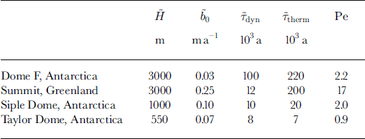
This ratio defines the trade-off between the advective and diffusive processes in the ice sheet. Temperature distributions in ice sheets with high Péclet numbers (thick, high accumulation rate, fast dynamic response times) are dominated by advection, while ice sheets with low Péclet numbers are dominated by conduction. Péclet numbers and characteristic times for several ice sheets are shown in Table 3.

Table 2.

Characteristic values used to non-dimensionalize Equation (29)

Table 3.

Characteristic values for specific ice sheets

Equation (29) or (30) is solved by the method of control volumes described by Reference PatankarPatankar (1980). A spatially uniform temperature is prescribed at the ice surface. A temperature gradient , determined by the geothermal heat flux q and the rock conductivity k _r, is uniformly prescribed 8 ice thicknesses below the bedrock/ice interface as recommended by Reference RitzRitz (1987). The horizontal temperature gradient is set to zero at the lateral boundaries of the domain.

Model Results: Isotherms

Figure 9 shows steady-state isotherms with no divide motion for ice sheets with different Péclet numbers when we use a non-linear ice-flow law (n = 3) to define the divide-zone flow. With divide migration, the isotherm shapes in the ice look qualitatively similar to the isochrone shapes shown in Figure 3, with steep slopes on the leading sides and shallow slopes on the trailing sides of isotherms. Figure 10 shows the depth distribution of the divide/flank temperature difference ΔT(z ) in the ice. The maximum temperature differences tend to occur near depths where the isochrone arches are also large. However, the temperature arch amplitudes are also controlled by the Péclet number, and are insensitive to the particular description of divide flow. Ice sheets with moderate Péclet numbers (Fig. 9a) are dominated by conduction, and the warming at the divide is apparent throughout the ice column. For advection-dominated ice sheets (high Péclet numbers), the temperature hot spot is concentrated at depth because fast downward advection of cold ice inhibits the upward diffusion of heat and tends to make the upper part of the ice sheet isothermal.

Fig. 9.

Isotherms (with non-linear ice dynamics) in units of Θ for an ice sheet with (a) low (Pe = 2) and (b) high (Pe = 20) Péclet numbers. Isotherms for divide flow from a local accumulation minimum are qualitatively similar.

Fig. 10.

Depth distribution of the divide temperature difference relative to flank ice for m = [0, 0.5, 1, 2, 4, 6, 10, 15]. (a) Pe = 2 and non-linear divide flow; (b) Pe = 20 and non-linear divide flow; (c) Pe = 2 and accumulation-low divide flow; and (d) Pe = 20 and accumulation-low divide flow.

There is a significant temperature signal at the ice/rock interface. Unlike isochrones, isotherms need not conform to the bed geometry. For a given set of parameters that govern ice flow ( , , h _f, h _d or , , Δb and W), the size of the temperature signal at the bed depends on the characteristic temperature (the temperature difference between the surface and bed in the absence of flow) and the Péclet number. As for isochrones, increasing divide motion progressively reduces the amplitude of the temperature signal ΔT because ice spends less time in the presence of divide flow for faster divide-motion rates.

The influence of diffusion in the bedrock is evident in the depth distribution of temperature amplitudes ΔT(x, z) for high migration rates. Figure 11 shows the temperature field for m = 0 and m = 6. With increasing migration rates, the region of warmest ice is spread horizontally behind the moving divide. Diffusion of heat through the ice and bedrock causes the divide temperature signature to vary slowly with depth across the ice/rock interface. This effect is clearly seen in ΔT amplitudes in Figure 10. At high migration rates, ΔT has little variation with depth in the deepest ice.

Fig. 11.

Distribution of the temperature hot spot ΔT (x, z) with non-linear divide flow and Pe = 20 for (a) m = 0, (b) m = 6. z = 0 is the ice/rock interface. Ten contour intervals in each panel show the shape of the temperature field. Contours do not correspond to the same temperatures in each panel. The heavy contour shows ΔT = 0.06 and ΔT = 0.01 for (a) and (b), respectively.

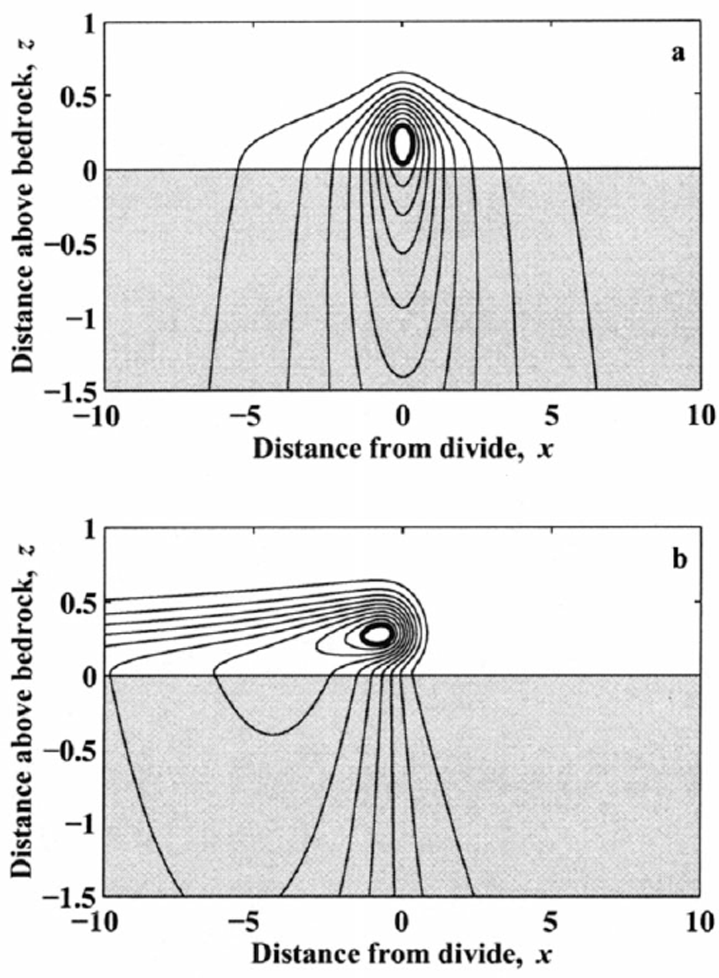
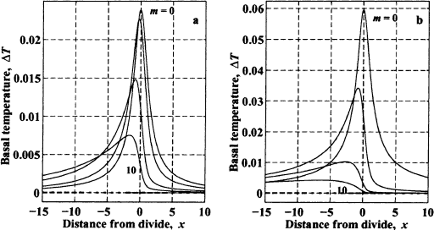
Figure 12 shows basal temperature variations (in units of the characteristic temperature Θ) for various migration rates for ice sheets with high and low Péclet numbers where the divide flow is caused by non-linear ice dynamics. As discussed in the next section, ice sheets with moderately high Péclet numbers (5–15) have the largest basal temperature signal. However, since ice sheets with high Pe values are dominated by advection, the temperature signal in the ice is carried away by ice flow faster than it is in ice sheets with low Péclet numbers. Warmest basal temperatures are offset a few ice thicknesses from the modern divide position.

Fig. 12.

Basal temperature pattern ΔT relative to flank in units of Θ for various divide-motion rates to the right (m = 0, 1, 4 and 10). (a) Low Péclet number (Pe = 2). (b) High Péclet number (Pe = 20). Dashed line denotes basal temperature in absence of divide effect. Divide flow results from ice nonlinearity with h_f = 0.2 and h_d = 0.6.

An Analytical Approach: Isotherms

The fundamental features of the heat-flow numerical model can be revealed with an analytical approach. We propose that a few dynamic ( and ) and thermal (Pe and Θ) parameters define the fundamental characteristics of isotherm shapes under a migrating divide.

Consider the one-dimensional heat-flow equation:

(32)

Assume the temperature field in the ice is initially at steady state consistent with flank-flow conditions. At , we impose a vertical velocity profile typical of divide flow so that , where is the flank-flow profile and . The associated temperature field is where is steady-state, consistent with flank flow, and is the perturbation due to divide flow. We assume and are small compared to the characteristic temperature Θ and velocity . Substituting these expressions in the one-dimensional heat equation and keeping only first-order terms yields

(33)

The last term in Equation (33) determines the magnitude of the temperature perturbation, but is not part of the transient solution. We use a scale analysis to estimate the characteristic time-scale of the transient perturbation in the ice. Substituting scale values (inverse length scale), and (average vertical velocity in the ice column) for ∂_z and , and solving for a characteristic time yields:

(34)

where Pe is the Péclet number. This characteristic time roughly represents the time it takes for the ice temperature to respond to a perturbation of the vertical velocity profile. Ice sheets that are advection-dominated (high Pe) have a faster thermal response time. However, this time-scale does not account for the associated temperature perturbation in the bedrock below the ice. When the temperature perturbation reaches the bed, warming the basal ice in the divide zone, the bedrock adjusts with a time-scale , where is the approximate width of the basal temperature perturbation (Reference WaddingtonWaddington, 1987). The transient temperature perturbation at the ice/rock interface is a combination of ice and rock response time-scales. Since for most ice sheets, thermal inertia of the bedrock tends to lengthen the total response time for basal temperatures.

Although this problem has more than one time constant, we can get an approximate analytical solution by assuming that the growth of the basal temperature signal associated with divide flow is exponential with a characteristic timescale given by a linear combination of and :

(35)

where f is the fractional contribution to the response time from and ΔT* is the steady-state flank–divide temperature difference at the bed with no divide migration.

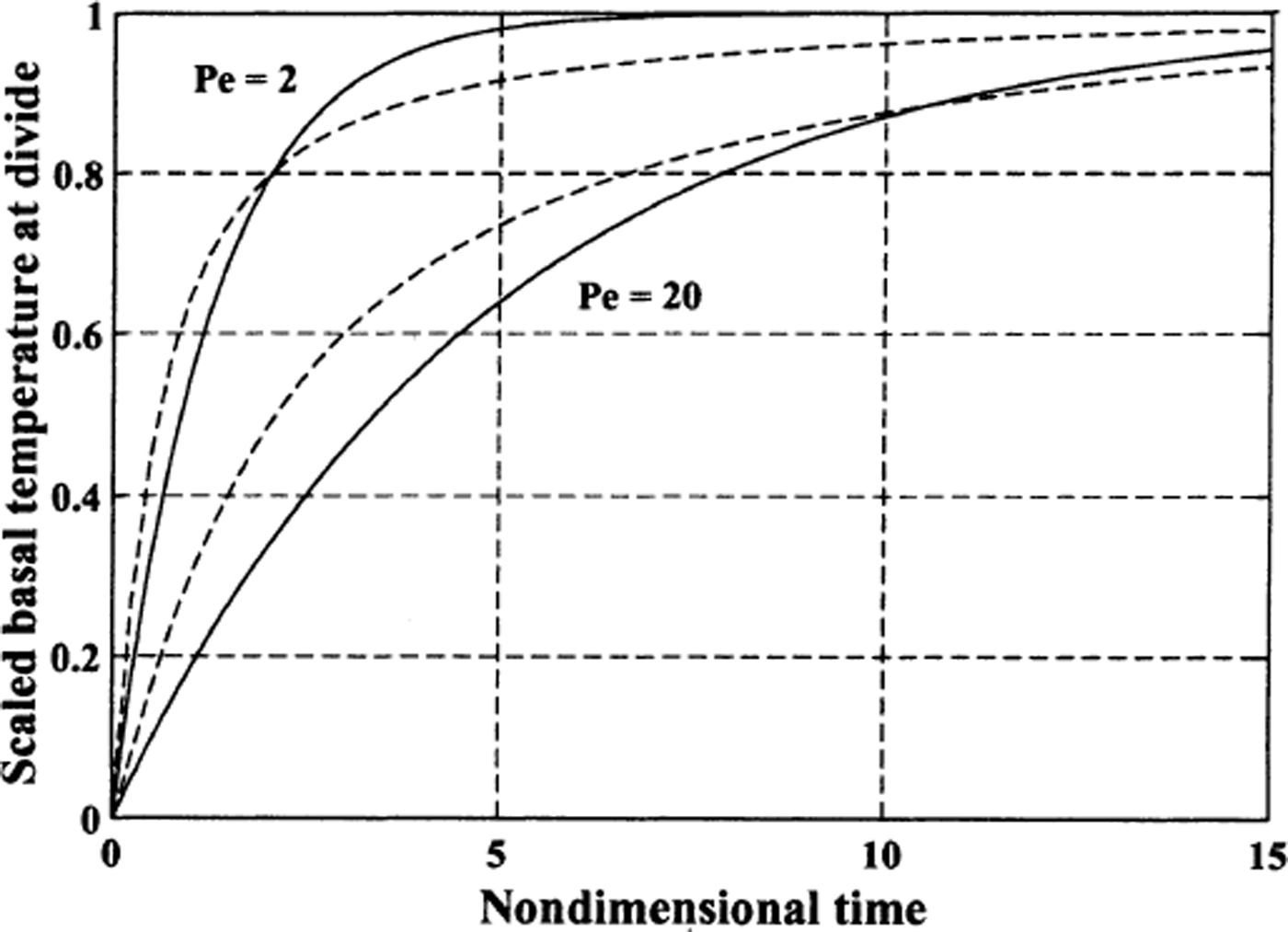
To estimate f, we use a time-dependent control-volume model to calculate the evolution of the basal temperature in an ice sheet initially at steady state with flank-flow conditions. Figure 13 shows how the basal temperature beneath the divide increases with time after a divide-flow regime is then imposed. Dashed lines show the evolution from the time-dependent, two-dimensional, control-volume model, and the solid lines show Equation (35) where f = 0.95 for both high and low Pe values. This combination of and gives a reasonable analytical approximation to the evolution time-scale. The time is typically much larger than , so its contribution to the evolution of basal temperature over the long-term temperature is significant, even though in Equation (35) its weight is only (1−f) =0.05.

Fig. 13.

Evolution of basal temperature at divide in units of the maximum temperature change ΔT* when divide flow is imposed on a steady-state temperature field consistent with flank flow everywhere. Dashed lines show results from the two-dimensional numerical model of heat flow for high and low Pe values. Solid lines show Equation (35) where ΔT* is taken from the numerical model and f = 0.95.

ΔT^* can be estimated from a steady one-dimensional temperature model for “Raymond” divide (h _d = 1) and “Nye” flank (h _f = 0) velocity regimes (Reference Firestone, Waddington and CunninghamFirestone and others, 1990; Reference PatersonPaterson, 1994, p. 218).

(36)

For accumulation scouring, ΔT^* can be estimated with a one-dimensional temperature model using “Nye” velocity regimes where the accumulation rate b = 1 for the flank site and b =(1 − Δb) for the divide site:

(37)

Figure 14 shows the basal temperature difference (relative to flank ice) given by Equations (36) and (37) for a range of Pe values. At the limit as Pe → 0 (no advection), the temperature difference approaches zero because there is no ice flow to differentiate the divide zone from the flank zone. With increasing Pe, the increased downward advection of cold ice on the flanks (compared to the divide zone) keeps the base relatively cold on the flanks. The maximum basal temperature difference occurs when Pe = 5–15. At larger Pe values, the increasingly strong downward advection of uniformly cold ice from the surface tends to make the ice sheet isothermal and inhibits the development of a divide temperature signal; as Pe → ∞, the temperature difference approaches zero everywhere.

Fig. 14.

Analytical estimate of basal temperature differences for various Pe values. Heavy line corresponds to “non-linear” divide zone with “Raymond” divide and “Nye” flank flow (Equation (36)). Light line corresponds to “accumulation minimum” divide zone with “Nye” divide (b = (1 −Δb)) and flank (b = 1) flow (Equation (37)) where Δb = 0.5.

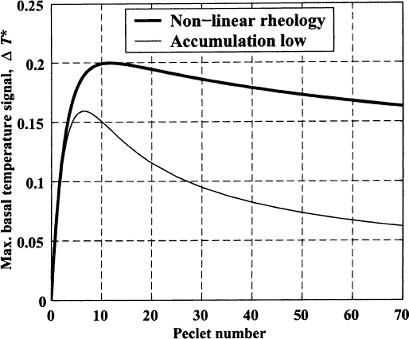
The magnitude of the temperature difference at the bed from Equation (36) (0.11 and 0.19 in units of Θ for Pe = 2 and 20) is about a factor of 2 higher than the difference predicted by the numerical model with the same divide and flank velocities (ΔT* = 0.05 and 0.11, respectively). This over-prediction results from the absence of horizontal diffusion in the one-dimensional temperature model. Since the width of the temperature hot spot is comparable to the ice thickness, the scale magnitudes of the horizontal and vertical diffusion terms are similar. This accounts for about a factor of 2 over-prediction of the temperature difference from Equations (36) and (37) (Reference Paterson and WaddingtonPaterson and Waddington, 1986).

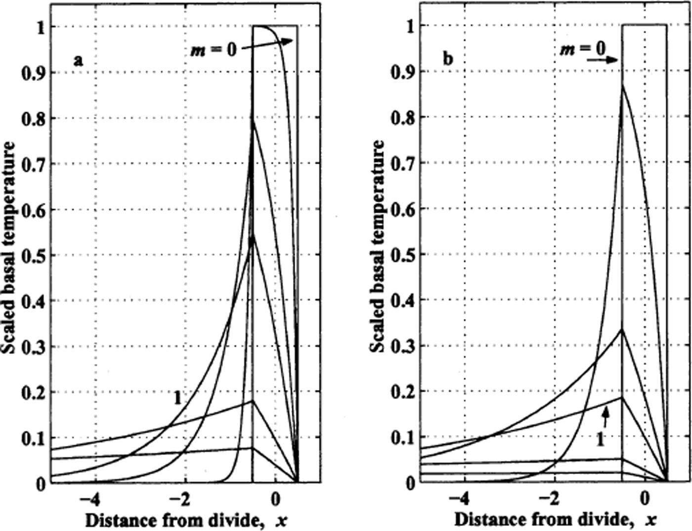
Just as for isochrones, we can imagine the divide zone as a moving “boxcar” in which the divide flow pattern is “on” and in which the divide thermal signal is allowed to grow according to Equation (35) while the divide zone is passing by ; after the divide zone passes by, the temperature decays with the same time constant as in Equation (35). Converting to the Lagrangian reference frame with the transformation (26) allows us to estimate the basal temperature difference (relative to flank ice) for two ice sheets with different Pe numbers and for various rates of divide migration (Fig. 15). The basal temperature is scaled to its maximum steady-state value to show how the shape of the basal temperature varies with m. These patterns show the same qualitative features seen in Figure 12. However, unlike the results shown in Figure 12, the magnitude of the divide temperature hot spot is dramatically reduced at even small migration rates. One possible explanation is that the actual width of the thermal divide zone is greater than because advection and diffusion processes spread the thermal effects of the dynamic divide zone. A wider thermal divide zone would allow more time for a basal temperature signal to develop as the divide passes by.

Fig. 15.

Analytical estimate of basal temperatures for (a) low Péclet number (Pe = 2) and (b) high Péclet number (Pe = 20) ice sheets for m = [0, 0.1, 0.5, 1, 4, 10].

Discussion

In order to characterize how isochrones or isotherms respond to divide motion, we have abstracted only those features of ice and heat flow that are essential to creating the arches, and not those features that might be unique to individual ice divides. By satisfying conservation laws and following widely recognized modeling approaches, our numerical models are quantitatively realistic approximations to this ideal, and we expect them to provide quantitatively realistic estimates of arch behaviors. Our analytical models, which are based on even simpler abstractions, cannot be expected to produce quantitatively reliable predictions of arch evolution throughout space and time. However, the fact that the analytical models show similar qualitative and quantitative behaviors to the numerical models gives strong confidence that the results of the numerical models should be broadly applicable to ice divides.

In our kinematic model, we assume that the velocity pattern is symmetric about the instantaneous flow divide, and the ice thickness does not change, despite the horizontal movement of the divide. In reality, flow divides occur at topographic crests, where slopes in opposite directions drive flow away from the divide. For a surface crest and its flow divide to migrate at rate while preserving its shape, there must be an asymmetric imbalance between the accumulation rate and the downward velocity pattern that thickens the ice sheet in the forward direction, and thins it behind. This asymmetric velocity imbalance must equal at the ice-sheet surface. For an ice sheet with thickness and span , near the divide is generally significantly smaller than . On typical ice sheets, is approximately 10⁻²−10⁻³, and we introduce an error significantly less than 1% into our downward velocity field when m is O(1). When m is larger, the instantaneous error in velocity can also be larger, but the ice spends less time in the divide zone, and the error in our calculated layer positions remains small. Continuity requires a small asymmetry in the corresponding horizontal velocity fields; however, since the isochrones and isotherms are sub-horizontal, this has negligible effect on their shapes. Therefore, this neglected but small asymmetric flow component that makes a divide migrate does not affect our conclusions.

Our analysis focuses on one type of divide motion: migration in one direction at a constant velocity. Other types of divide motion include acceleration, changes in direction, or random motion of the divide position. Reference HindmarshHindmarsh (1996) shows how random stochastic motion of the ice divide can eliminate the perceptible signature of divide flow in the internal layer shapes. Reference Nereson and RaymondNereson and Raymond (2001) invoke fast motion of the ice divide to explain the absence of divide signatures at ridge BC, West Antarctica. They also invoke small-amplitude oscillations in divide position to explain the wide divide arches at ridge DE. The analysis that we report here can be viewed as the basic building-blocks for these more complex behaviors.

For isochrones, the divide arch amplitude Δz(z) depends on n with a non-linear constitutive law, or on Δb for accumulation scouring. The size of the thermal signal ΔT(z) depends on Pe; the largest ΔT values are associated with Pe ≈ 5–15. With divide motion, the size of the signal is reduced. At low migration rates, m < 1, the time that a given column of ice spends in the divide zone is greater than the time for vertical motion. Most ice in the divide zone resides there for a time comparable to its age. Therefore, slow divide motion has little effect on the isochrone and isotherm arch amplitudes for ice sheets with low Péclet numbers. When m > 1, ice spends less time than in the divide zone; this inhibits the development of an isochrone arch. Ice sheets with high Péclet numbers are a special case. They have a slow thermal response time compared to . Even with very slow divide motion m ≪ 1, the ice column does not have enough time to develop a thermal hot spot to near its steady-state value (see Fig. 10).

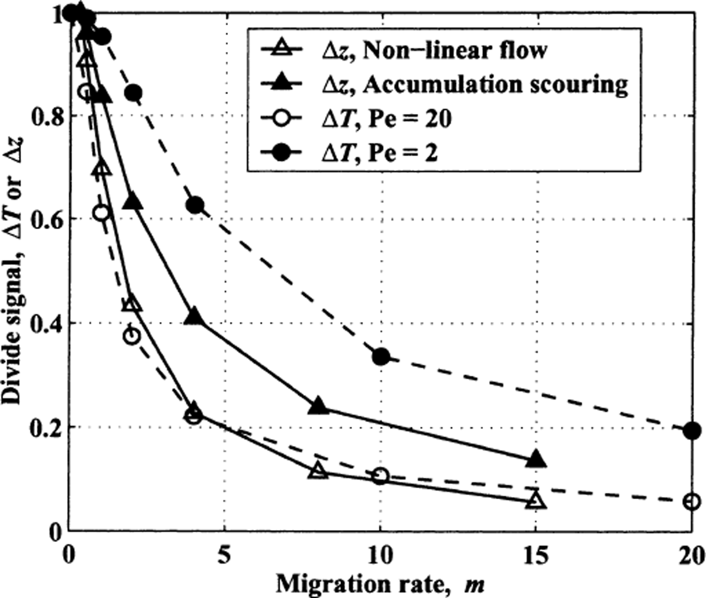
Figure 16 shows how the divide signal, either isochrone arch amplitude (max[Δz(z)]) or basal temperature difference (max[ΔT(z)]), varies with migration rate. The divide signal decreases with increasing migration rates, with an e-folding m value of about 3–5. The e-folding migration rate for basal temperature anomalies is higher for ice sheets with low Péclet numbers. These ice sheets have a relatively fast thermal response time so that basal ice temperatures beneath the divide can approach steady-state values even when the divide is moving relatively fast. However, ice sheets with low Péclet numbers tend to be thinner and have smaller temperature anomalies than ice sheets with high Péclet numbers. Therefore, even though ice sheets with low Péclet numbers retain the temperature signal for faster migration rates, the absolute value of the signal may be more difficult to detect.

Fig. 16.

Scaled amplitude of thermal signal (ΔT: dashed lines) or isochrone arch (Δz: solid lines) vs divide-migration rate. ΔT is shown for high (Pe = 20 (●)) and low (Pe = 2(○)) Péclet numbers assuming flow conditions as in Figure 10a and b. Scaled Δz values are shown for non-linear flow (Δ) and accumulation scouring (▲) vs migration rate. Flow conditions as in Figure 4.

Since different characteristic times govern the development of isochrone and isotherm arches, it may be possible to use measurements of isotherms and isochrones together to extend the measurable record of divide migration. If the response time is fast, then the isochrones or isotherms can record a divide signal even if the divide is moving rapidly. If the response time is slow, then the isochrones or isotherms may not have enough time in the divide zone to develop a detectable arch before the divide passes by. The important time-scales are the age of the ice for isochrones and (Equation (34)) for isotherms. At a height z where age , the ratio /age is greater than unity when Pe > 2.

For high Péclet numbers, the thermal response time is slower (larger ) than the isochrone arch-growth response time, and the isochrone shapes record a longer history of divide position than the temperature signal. In this case, it may be possible to determine the long-term average divide-motion rate from isochrone shapes, and the more recent divide-motion rate from basal temperatures. A comparison would allow detection of changes in the divide-migration rate over time.

For very low Péclet numbers, the situation is reversed so that the temperature signal has a faster response time than the isochrone arch. In this case, the temperatures record a longer history of divide position, and measurements of temperatures may extend the record of divide-motion history as inferred from isochrone shapes. Measuring ice temperatures at enough points and depths to be useful is currently beyond our ability to achieve at a reasonable cost. However, when the capability to drill low-cost access holes is developed, this would be a promising application at divides with low Pe values.

Conclusions

Simple numerical and analytical models reveal the general characteristics of arched isochrones and isotherms beneath moving ice divides. The isochrones and isotherms are asymmetric, with steep slopes on their leading edges and shallow slopes on their trailing sides. This asymmetry is due to (1) total time the ice is exposed to divide flow, (2) the relaxation of the divide signal since divide passage, and (3) the horizontal strain that moves and stretches the arches. The magnitude of the signal depends on n or Δb for isochrones and also on Θ and Pe for isotherms.

For isochrones, the arch amplitude given a steady divide-migration rate m can be estimated from Equation (21) or (25) for non-linear or accumulation-low divide flow, respectively. The position of the arch can be estimated from Equation (28). Basal temperatures under steady divide motion can be roughly estimated from Equation (35), but neglect of horizontal heat flow leads to an over-prediction by about a factor of 2.

The amplitude of the arch is similar to its steady-state value for m < 1, when deformation from vertical ice flow dominates and effects for horizontal motion of the divide are small. At higher m values, the amplitude of the isochrone arch or temperature signal decreases with an e-folding value of m ∼ 3–5. Temperatures may record a longer history of divide position than isochrone shapes for ice sheets where Pe ∼ 2 or less. Otherwise, isochrone shapes record a longer history of divide motion. Of course, to apply these concepts at specific sites will require detailed numerical models with specific geometric, dynamic and thermal parameters.