


1. Introduction
Climate change poses growing challenges to agricultural production (Luchtenbelt et al., Reference Luchtenbelt, Doelman, Bos, Daioglou, Jägermeyr, Müller, Stehfest and van Vuuren2024). Droughts, floods, storms, and other weather-related hazards can directly disrupt crop growth and reduce yields, while increasing climatic variability further amplifies production uncertainty. For staple crops such as maize, wheat, and rice, yields are expected to fluctuate more substantially under changing climatic conditions (Rezaei et al., Reference Rezaei, Webber, Asseng, Boote, Durand, Ewert, Martre and MacCarthy2023), and extreme events may even result in complete crop failure. These developments have made climate risk management increasingly important for safeguarding agricultural production and supporting policy responses at broader regional scales. This need is particularly evident in agricultural systems characterized by strong spatial aggregation. Crop production is unevenly distributed across counties, and output in major producing counties contributes disproportionately to overall state-level production. Consequently, state-level climate risk management cannot rely solely on aggregate information, nor can county-level decisions be made in isolation. Effective allocation of disaster-prevention resources and climate adaptation measures, therefore, requires forecasts that are not only accurate at the county level but also coherent with state-level production outcomes. This naturally calls for hierarchical forecasting approaches that ensure cross-level consistency. Existing studies have mainly examined the effects of weather conditions on crop yields within individual regions and have shown that wheat is particularly sensitive to weather conditions at different stages of the growing cycle (Tan et al., Reference Tan, Wu and Zhao2017; Zhao et al., Reference Zhao, Liu, Piao, Wang, Lobell, Huang, Huang, Yao, Bassu, Ciais, Durand, Elliott, Ewert, Janssens, Li, Lin, Liu, Martre, Müller and Asseng2017; Sun et al., Reference Sun, Yang, Zhang, Zhao and Liu2021; Meng et al., Reference Meng, Wang, Yao, Qian, Chen, Luo and Ju2022). Some studies have developed yield forecasting models using a limited number of key weather variables, such as temperature and precipitation during the growing season (Liu et al., Reference Liu, He, Wang and Huang2019; He et al., Reference He, Luo, Qiao, Tian and Zhou2021; Bangelesa et al., Reference Bangelesa, Pollinger, Sponholz, Mapatano, Hatloy and Paeth2023; Zhang et al., Reference Zhang, Gong, He and Huo2023), while others have focused on variable selection methods (Bai & Ng, Reference Bai and Ng2002; Li et al., Reference Li, Porth, Tan and Zhu2021). Despite these efforts, it remains difficult to forecast current-year crop yields accurately under changing climatic conditions, quantify yield risk, and manage weather-related risk when climatic disasters occur.
Quantitative measurement of crop yield risk presents unique challenges. First, the limited availability of yield data constrains empirical modeling and robust statistical inference of yield distributions, as yield and loss observations are typically recorded only once per year and may occasionally suffer from missing values (Ramsey, Reference Ramsey2020). Second, the presence of spatial and temporal correlations in the data-generating process complicates crop yield forecasting. Failure to account for these dependencies may lead to biased or misleading estimates of yield risk (Ramsey, Reference Ramsey2020; Liu & Ker, Reference Liu and Ker2021). Meanwhile, weather-related risk plays a critical role in both crop yield forecasting and risk management. Research has shown that incorporating weather covariates, rather than relying solely on historical yield data, can substantially improve the accuracy and reliability of crop yield models (Lobell et al., Reference Lobell, Schlenker and Roberts2011; Kleiber et al., Reference Kleiber, Raftery and Gneiting2011). However, integrating weather variables into crop-yield forecasting and risk assessment models presents several significant challenges. On the one hand, weather data are rich and high-dimensional, which makes dimensionality reduction challenging, particularly given the typically short time series of available yield data (Li et al., Reference Li, Porth, Tan and Zhu2021). On the other hand, systemic weather risks, which exhibit spatial correlations across large geographic regions, often result in highly variable year-to-year losses, thereby complicating the accurate quantification of crop yield risk (Zhu et al., Reference Zhu, Tan, Porth and Wang2018). Moreover, coherence in yield statistics matters not only for official reporting but also for insurance design and risk management. The U.S. National Agricultural Statistics Service (NASS) places considerable weight on consistency in reported yields across counties, states, and the nation. Through benchmarking procedures and hierarchical aggregation constraints, published estimates are made internally consistent across reporting levels and comparable across commodities under common definitions (Summary and Disclosure Methodology Branch, 2023). Coherence is also important at the contract level. Area-based crop insurance programs such as the Group Risk Plan (GRP) base indemnities on a county yield index rather than on an individual producer’s realized yield.Footnote 1 As a result, contract outcomes depend on an external and publicly reported measure that cannot be manipulated by individual policyholders. For insurers, premium rating and risk management, therefore, require yield data that are consistent across levels of aggregation so that county-level pricing remains aligned with portfolio accounting at the state and national levels (Ker et al., Reference Ker, Tolhurst and Liu2016). In this setting, coherence is not only a statistical property of yield data. It is also essential to use area yield indices in pricing, reserving, and reinsurance. Only when yield measures are coherent within the hierarchy can insurers connect county-level pricing decisions to portfolio loss distributions, economic capital assessment, and reinsurance pricing in a unified framework (Meyers, Reference Meyers2001; Meyers et al., Reference Meyers, Klinker and Lalonde2003; Chong et al., Reference Chong, Feng and Jin2023; Guan et al., Reference Guan, Tsanakas and Wang2023).
In hierarchical yield forecasting, it is necessary to construct separate models for each level of the hierarchy. However, discrepancies among these models may lead to inconsistencies across forecast values across hierarchical levels, thereby violating the principle of hierarchical coherence. Forecast reconciliation is a statistical technique for adjusting hierarchical time-series forecasts to ensure consistency with the underlying hierarchical structure (Wickramasuriya et al., Reference Wickramasuriya, Athanasopoulos and Hyndman2019). When addressing the forecasting problem of hierarchical time series, it remains standard practice to model and predict the output at each level independently. Although there is a theoretical aggregation relationship among forecasts at different levels, using distinct optimal models across levels often yields incoherent results that fail to preserve this structure. Forecast reconciliation methods offer a systematic solution to this issue by aligning forecasts across levels in a statistically optimal manner. One of the earliest reconciliation approaches introduced in the literature is the Bottom-Up (BU) method, which aggregates forecasts from the most disaggregated (bottom) level to obtain higher-level forecasts (Orcutt et al., Reference Orcutt, Watts and Edwards1968; Dunn et al., Reference Dunn, Williams and DeChaine1976). Building upon the Generalized Least Squares (GLS) reconciliation framework proposed by Hyndman et al. (Reference Hyndman, Ahmed, Athanasopoulos and Shang2011), Wickramasuriya et al. (Reference Wickramasuriya, Athanasopoulos and Hyndman2019) introduced the Minimum Trace (MinT) reconciliation method, which improves the estimation of the inverse covariance matrix to achieve more accurate forecast reconciliation. The MinT approach obtains coherent forecasts for hierarchical time series by minimizing the total variance of forecast errors after reconciliation. To date, this method has been successfully applied in various domains, including electricity demand forecasting (Taieb et al., Reference Taieb, Taylor and Hyndman2021) and population mortality projections (Li et al., Reference Li, Li, Lu and Panagiotelis2019). However, it has yet to be explored in the context of agricultural production forecasting.
However, a key limitation of point forecasts is their inability to convey uncertainty about future outcomes. As a result, they provide no insight into the potential variability or risk associated with forecast errors, thereby limiting their usefulness in decision-making. To address this issue, probabilistic forecasts, which represent future quantities of interest as full probability distributions rather than single-point estimates, have been increasingly adopted across a wide range of fields. A widely used framework for generating density forecasts independently across hierarchical time series has been introduced in previous work (Hyndman et al., Reference Hyndman, Ahmed, Athanasopoulos and Shang2011). This approach enables large-scale probabilistic forecasting and ensures that the forecast distribution of any aggregated series equals the convolution of the distributions of its components, thus preserving hierarchical coherence. Moreover, point forecasts are inherently limited to providing a single estimate for each time step. In contrast, when the incoherent base forecast distributions are assumed to be jointly Gaussian, it is possible to fully leverage the relationship between point forecasts and forecast errors to construct prediction intervals and evaluate forecast performance using proper scoring rules or loss functions. This highlights the added value of probabilistic forecasts in capturing forecast uncertainty and enhancing decision support. Applications include meteorology (Leutbecher, Reference Leutbecher2019), energy (Taieb et al., Reference Taieb, Huser, Hyndman and Genton2016), and retail forecasting (Berry et al., Reference Berry, Helman and West2020).
The objective of this study is to develop an integrated measurement framework to improve crop yield forecasting and risk assessment, thereby supporting more effective agricultural risk management and facilitating multi-regional risk zoning. To achieve this, we propose integrating high-dimensional weather variables, after applying dimensionality reduction techniques, into a probabilistic forecasting framework. This approach aims to improve both the accuracy and hierarchical coherence of hierarchical crop yield predictions. Specifically, this paper has the following marginal contributions. First, this study develops an ensemble yield forecasting model that identifies key weather-related risk factors and evaluates forecasting accuracy at multiple levels. The findings provide empirical support and methodological guidance for the design of crop insurance products and the formulation of data-informed weather risk management strategies in agriculture. Second, the proposed risk measurement framework contributes a generalizable approach to crop yield risk management. Utilizing the median of probabilistic forecasts offers an effective means of capturing and optimizing tail risks, thereby enhancing the robustness of agricultural risk assessment across different crop types. Moreover, when weather data are scarce or unavailable, forecast reconciliation techniques can partially compensate for the resulting loss in accuracy, thereby enabling reliable yield predictions while reducing data acquisition costs. Finally, the framework was applied to real crop yield insurance ratemaking by conducting a retain–cede rating game between a private insurer and the government (Ker & McGowan, Reference Ker and McGowan2000; Harri et al., Reference Harri, Coble, Ker and Goodwin2011; Zhang, Reference Zhang2017; Ramsey, Reference Ramsey2020; Liu & Ker, Reference Liu and Ker2021; Zhu, Reference Zhu2024).
The remainder of this paper is organized as follows. Section 2 describes the wheat and weather data used in this paper and constructs a hierarchical time series of two types of wheat in Montana. Section 3 starts from the point forecast and probability forecast models and introduces in detail the forecasting framework. In Section 4, an empirical study of two types of wheat in Montana is conducted based on the forecast models above. In Section 5, the proposed forecasting framework is applied to a crop insurance rating game. Section 6 concludes the article.
2. Data
Our empirical analysis is based on county-level wheat yield data and county-level monthly climate data for Montana, United States. These two datasets differ substantially in both temporal frequency and spatial structure. Wheat yield is measured annually, consistent with the harvest cycle, whereas climate variables are observed monthly. At the same time, the yield data exhibit a hierarchical structure that can be aggregated from the county level to crop-specific and state-level series, while the climate data are defined at the county administrative level. The key data-construction challenge is therefore to transform high-frequency county-level climate observations into county-year measures that align with annual wheat yield outcomes while preserving spatial consistency. In addition, because the resulting climate covariates are high-dimensional, we further apply principal component analysis (PCA) in the subsequent modeling stage to reduce dimensionality.
Hierarchical structure of crop yield.

2.1 U.S. wheat data
Wheat yield data used in this study were obtained from the Quick Stats database maintained by the National Agricultural Statistics Service of the United States Department of Agriculture (USDA NASS).Footnote
2
The empirical dataset covers 51 Montana counties, and both spring wheat and winter wheat are cultivated across the state. Accordingly, the yield data have a natural hierarchical structure with three levels: state, wheat category (spring versus winter), and county. Figure 1 illustrates this hierarchy, from total state yield to disaggregated county-level series. In the empirical analysis, annual spring wheat yield is denoted by $\boldsymbol{y}_s$
, annual winter wheat yield by
$\boldsymbol{y}_s$
, annual winter wheat yield by $\boldsymbol{y}_w$
, and aggregate annual wheat yield by
$\boldsymbol{y}_w$
, and aggregate annual wheat yield by $\boldsymbol{y}_T$
. This structure allows us to analyze wheat dynamics at both disaggregated and aggregated levels.Footnote
3
Because the original yield dataset contains missing observations, we use interpolation methods to impute the missing values.
$\boldsymbol{y}_T$
. This structure allows us to analyze wheat dynamics at both disaggregated and aggregated levels.Footnote
3
Because the original yield dataset contains missing observations, we use interpolation methods to impute the missing values.
2.2 U.S. weather data
The county-level monthly climate data for Montana are drawn from NASA’s Prediction of Worldwide Energy Resources (POWER) project.Footnote
4
The dataset provides a distinct monthly climate time series for each county over 1982–2022. Climate variables are therefore defined at the county administrative level, and their realized values are county-specific, ensuring spatial alignment with county-level yield observations. These monthly climate observations are aggregated into county-year, crop-specific growing-season measures before being matched to annual yield data by county and year. Because spring wheat and winter wheat differ in their biological growing cycles, climate variables are constructed separately for each crop using crop-specific growth windows. For winter wheat, the relevant growth period spans October of year $t-1$
through June of year
$t-1$
through June of year $t$
(9 months), whereas for spring wheat it spans March through August of year
$t$
(9 months), whereas for spring wheat it spans March through August of year $t$
(6 months). Table 1 lists all climate variables included in the analysis. Accordingly, we construct 174 climate variables for spring wheat and 290 for winter wheat, each based on monthly observations within the corresponding growth period.
$t$
(6 months). Table 1 lists all climate variables included in the analysis. Accordingly, we construct 174 climate variables for spring wheat and 290 for winter wheat, each based on monthly observations within the corresponding growth period.
Climate-related variables

3. Model and methodology
This section outlines the overall framework for forecasting agricultural yield and quantifying yield risk under climate change. Section 3.1 reviews common modeling approaches that leverage mixed-frequency data for yield prediction. Section 3.2 discusses methods for achieving coherence in forecasts across spatial hierarchies. Section 3.3 introduces key concepts used to generate probabilistic forecast samples for quantifying yield risk under climate change. Section 3.4 describes the modeling pipeline and implementation steps.
The classical literature primarily employs yield decomposition models to empirically assess agricultural productivity. These models separate historical yields into two components: weather-driven yields and trend yields. Building on this foundation, we reconstruct the analytical framework (Coulombe et al., Reference Coulombe, Marcellino and Stevanović2021) as follows:
 \begin{align*} \min _{g \in \mathcal{G}}\left \{\sum _{t=1}^{T}\left (y_{t}-\hat {y}_{t}\right )^2\right \}=\min _{g \in \mathcal{G}}\left \{\sum _{t=1}^{T}\left (y_{t}-T(y_{t})-g\left (\boldsymbol{X}_{t}\right )\right )^2\right \}, \end{align*}
where $y_{t}$
denotes the observed historical yield, and
$y_{t}$
denotes the observed historical yield, and $\hat {y}_{t}$
represents the fitted yields. The yield is decomposed into two components, the trend yield
$\hat {y}_{t}$
represents the fitted yields. The yield is decomposed into two components, the trend yield $T(y_{t})$
, and the weather-induced yield
$T(y_{t})$
, and the weather-induced yield $g(\boldsymbol{X}_{t})$
, where the function
$g(\boldsymbol{X}_{t})$
, where the function $g$
, selected from a functional space
$g$
, selected from a functional space $\mathcal{G}$
, maps the transformed climate covariates
$\mathcal{G}$
, maps the transformed climate covariates $\boldsymbol{X}_{t}$
to yield outcomes. Based on this framework, we present three modeling approaches that differ in the degree of decomposition applied to yield dynamics.
$\boldsymbol{X}_{t}$
to yield outcomes. Based on this framework, we present three modeling approaches that differ in the degree of decomposition applied to yield dynamics.
3.1 Base forecasting methods
3.1.1 ARIMA
External weather conditions are critical determinants of wheat production. Incorporating weather variables into the ARIMA framework yields a dynamic regression model (ARIMAX), which improves forecasting accuracy by leveraging exogenous climatic information.
Assuming there are $u$
weather factors, represented by
$u$
weather factors, represented by $y_t$
as the wheat yield at time point
$y_t$
as the wheat yield at time point $t$
,
$t$
, $\phi _i$
as the coefficient of the auto-regressive term,
$\phi _i$
as the coefficient of the auto-regressive term, $B$
as the regression operator,
$B$
as the regression operator, $\theta _j$
as the coefficient of the moving average term,
$\theta _j$
as the coefficient of the moving average term, $\mathbf{X}_{k,t}$
as the
$\mathbf{X}_{k,t}$
as the $k$
-th weather factors at time point
$k$
-th weather factors at time point $t$
, and
$t$
, and $\beta _k$
as the regression coefficient corresponding to the weather factors
$\beta _k$
as the regression coefficient corresponding to the weather factors $\mathbf{X}_{k,t}$
, the ARIMAX model of crop yield with weather factors is represented as follows:
$\mathbf{X}_{k,t}$
, the ARIMAX model of crop yield with weather factors is represented as follows:
 \begin{align*} y_{t}=\frac {(1+\sum _{j=1}^{q}\theta _jB^{\,j})\varepsilon _t+\sum _{k=1}^{u}\beta _kX_{k,t}}{(1-\sum _{i=1}^{p}\phi _iB^i)(1-B)^d}, \end{align*}
where $p$
and
$p$
and $q$
are the order of the model,
$q$
are the order of the model, $d$
is the differential order,
$d$
is the differential order, $u$
is the number of weather variables, and
$u$
is the number of weather variables, and $\varepsilon _t$
is the error term.
$\varepsilon _t$
is the error term.
3.1.2 Mixed frequency data sampling (MIDAS) regression
Mixed frequency data sampling (MIDAS) regression is designed to accommodate time series data observed at different temporal resolutions. Unlike traditional models that require data aggregation or latent factor extraction, MIDAS allows high-frequency covariates to directly inform the prediction of a low-frequency target variable. In this study, we employ a fixed single-equation MIDAS regression with an autoregressive component, where the dependent variable is measured annually, and the explanatory variables are sampled five times per year. The model is specified as follows:
 \begin{align*} y_{t}=\alpha +\sum _{i=1}^{p}\beta _iL^iy_t+\gamma \sum _{k=1}^{q}\Phi \left (k;\,\theta \right )L_{HF}^qX_{ct-k}+\varepsilon _t, \\[-30pt] \end{align*}
where $L_{HF}$
denotes the high-frequency lag operator,
$L_{HF}$
denotes the high-frequency lag operator, $q$
is the high-frequency alignment indicator, and
$q$
is the high-frequency alignment indicator, and $\Phi (k;\,\theta )$
is the weighting operator applied to the mixed-frequency weather factors
$\Phi (k;\,\theta )$
is the weighting operator applied to the mixed-frequency weather factors $X_{ct-k}$
. The subscript
$X_{ct-k}$
. The subscript $c$
in
$c$
in $ct-k$
denotes the high-frequency position relative to the low-frequency period
$ct-k$
denotes the high-frequency position relative to the low-frequency period $t$
. Moreover,
$t$
. Moreover, $\alpha$
denotes the intercept term of the model, while
$\alpha$
denotes the intercept term of the model, while $\gamma$
represents the overall coefficient (or scaling parameter) associated with the weighted high-frequency explanatory component. Accordingly, the model employed in this article is a MIDAS-AR model.
$\gamma$
represents the overall coefficient (or scaling parameter) associated with the weighted high-frequency explanatory component. Accordingly, the model employed in this article is a MIDAS-AR model.
3.1.3 Neural network models
Extensive research has been conducted on a wide range of machine learning algorithms, which offer flexible modeling tools aimed at minimizing expected prediction loss. Among these, feed-forward neural networks (FFNN) are particularly effective in capturing complex nonlinear relationships between climate variables and agricultural yields, without requiring a priori specification of functional forms. Compared to traditional linear models and tree-based approaches, FFNN offer greater flexibility in learning intricate patterns from high-dimensional data. This advantage becomes especially critical when dealing with heterogeneous and uncertain climate conditions. Given that the dataset used in this study incorporates exogenous weather variables, we adopt the FFNN framework to examine the potential of machine learning in enhancing the accuracy of real-time crop yield forecasting.
Neural networks, based on the structural principles of the human brain, are computational frameworks that reproduce the architecture of biological neural systems. Among them, the FFNN is one of the most commonly used types of artificial neural networks. Figure 2 provides an example of FFNN. A defining characteristic of FFNN is their acyclic structure, meaning connections between nodes do not form feedback loops. The network processes crop yield historical observations through successive hidden layers, where each neuron applies a weighted transformation followed by a nonlinear activation function. In addition to yield history, the model incorporates exogenous weather factors as supplementary inputs. These weather factors (xreg1-xregK) serve as forecasts that capture the influence of climatic conditions on crop yield. The outputs from the hidden layers are combined to generate the final forecasts of crop yield in the output layer.
Feed-forward neural networks for forecasting crop yield.

Figure 2 Long description
A diagram of a feed-forward neural network for forecasting crop yield. The diagram shows input nodes labeled xreg1, xreg2, ..., xregK, and y_t...y_{t-T}, which are connected to hidden layer nodes labeled H1, H2, ..., H(p-1), and Hp. These hidden layer nodes are then connected to an output node labeled y_{t+1}. The arrows indicate the direction of data flow from the input nodes through the hidden layers to the output node.
3.2 Hierarchical forecast reconciliation
Accurate forecasting of wheat yields in a hierarchical system requires forecasts that are not only individually reasonable at each level but also mutually consistent with the underlying aggregation structure. Forecast reconciliation provides a statistical framework for adjusting a set of base forecasts so that coherence is achieved across spatial or categorical hierarchies (Zellner & Tobias, Reference Zellner and Tobias2000). In this paper, a hierarchical time series is defined as an $n$
-dimensional multivariate time series subject to known linear aggregation constraints, where lower-level county series aggregate to higher-level series such as crop-specific totals and overall yield.
$n$
-dimensional multivariate time series subject to known linear aggregation constraints, where lower-level county series aggregate to higher-level series such as crop-specific totals and overall yield.
Let $\boldsymbol{y}_t\in \mathbb{R}^{\textit {m}}$
be a vector comprising observations from all time series in the hierarchy at time t, and
$\boldsymbol{y}_t\in \mathbb{R}^{\textit {m}}$
be a vector comprising observations from all time series in the hierarchy at time t, and $\boldsymbol{b}_t\in \mathbb{R}^{n}$
be a vector comprising observations of only the most disaggregated (bottom-level) series. The full hierarchy can be written as
$\boldsymbol{b}_t\in \mathbb{R}^{n}$
be a vector comprising observations of only the most disaggregated (bottom-level) series. The full hierarchy can be written as
 \begin{align*} \boldsymbol{y}_t = \boldsymbol{S}\boldsymbol{b}_t. \end{align*}
When the summing matrix $\boldsymbol{S}\in \mathbb{R}^{m \times n}$
linearly aggregates base-level observations to higher hierarchy levels. Define
$\boldsymbol{S}\in \mathbb{R}^{m \times n}$
linearly aggregates base-level observations to higher hierarchy levels. Define $\boldsymbol{A}\in \mathbb{R}^{(m-n) \times n}$
as an
$\boldsymbol{A}\in \mathbb{R}^{(m-n) \times n}$
as an $(m-n) \times n$
aggregation matrix with
$(m-n) \times n$
aggregation matrix with $n = n_a +n_b$
, and
$n = n_a +n_b$
, and $I_{n}$
is an
$I_{n}$
is an $n$
-dimensional identity matrix, then
$n$
-dimensional identity matrix, then
 \begin{align*} \boldsymbol{S}= \begin{bmatrix} \boldsymbol{A} \\ {\boldsymbol{I}_{\boldsymbol{n}}} \end{bmatrix}_{m \times n}. \end{align*}
For example, according to the hierarchical structure of wheat in Montana, $n_a=n_b=51, n=102, m=105$
,
$n_a=n_b=51, n=102, m=105$
, $\boldsymbol{y}_t=[\boldsymbol{y}_T,\boldsymbol{y}_S,\boldsymbol{y}_W,\boldsymbol{y}_s^1,\ldots ,\boldsymbol{y}_s^{51},\boldsymbol{y}_w^1,\ldots ,\boldsymbol{y}_w^{51}]^{'}$
is a series matrix of wheat yields at all levels,
$\boldsymbol{y}_t=[\boldsymbol{y}_T,\boldsymbol{y}_S,\boldsymbol{y}_W,\boldsymbol{y}_s^1,\ldots ,\boldsymbol{y}_s^{51},\boldsymbol{y}_w^1,\ldots ,\boldsymbol{y}_w^{51}]^{'}$
is a series matrix of wheat yields at all levels, $\boldsymbol{b}_t=[\boldsymbol{y}_s^1,\ldots ,\boldsymbol{y}_s^{51},\boldsymbol{y}_w^1,\ldots ,\boldsymbol{y}_w^{51}]^{'}$
is a series matrix of two wheat yield observations in 51 counties. The aggregation matrix
$\boldsymbol{b}_t=[\boldsymbol{y}_s^1,\ldots ,\boldsymbol{y}_s^{51},\boldsymbol{y}_w^1,\ldots ,\boldsymbol{y}_w^{51}]^{'}$
is a series matrix of two wheat yield observations in 51 counties. The aggregation matrix $A$
can be written as
$A$
can be written as
 \begin{align*} \boldsymbol{A}= \begin{bmatrix} \overbrace {1 \ \cdots \ 1 \ 1 \ \cdots \ 1}^{n=102} \\ \overbrace {1 \ \cdots \ 1 }^{n_a=51} \overbrace {\ 0 \ \cdots \ 0}^{n_b=51} \\ \underbrace {0 \ \cdots \ 0}_{n_a=51} \underbrace {\ 1 \ \cdots \ 1}_{n_b=51} \\ \end{bmatrix}_{3 \times 102}. \end{align*}
The $h$
-step-ahead base forecasts are generated independently across the hierarchical structure, thus necessitating a reconciliation process to adjust them through cross-level information integration, which enhances alignment with observed values while maintaining aggregation coherence.
$h$
-step-ahead base forecasts are generated independently across the hierarchical structure, thus necessitating a reconciliation process to adjust them through cross-level information integration, which enhances alignment with observed values while maintaining aggregation coherence.
Let $\widehat {\boldsymbol{y}}_{t+h|t}$
represent the
$\widehat {\boldsymbol{y}}_{t+h|t}$
represent the $h$
-step-ahead base forecasts for each series in the structure, and
$h$
-step-ahead base forecasts for each series in the structure, and $\widetilde {\boldsymbol{y}}_{t+h|t}$
represent the
$\widetilde {\boldsymbol{y}}_{t+h|t}$
represent the $h$
-step-ahead forecast of each time series after reconciliation. All linear reconciliation methods can be expressed as
$h$
-step-ahead forecast of each time series after reconciliation. All linear reconciliation methods can be expressed as
 \begin{equation} {\widetilde {\boldsymbol{y}}}_{t+h|t}=\boldsymbol{S}\boldsymbol{G}\,{\widehat {\boldsymbol{y}}}_{t+h|t} , \end{equation}
where $\boldsymbol{S}$
is the summing matrix and
$\boldsymbol{S}$
is the summing matrix and $\boldsymbol{G}$
is the weight matrix,
$\boldsymbol{G}$
is the weight matrix, $\boldsymbol{SG}$
can be treated as the projection matrix. The transformation, in the most general case, is a mapping
$\boldsymbol{SG}$
can be treated as the projection matrix. The transformation, in the most general case, is a mapping $\psi$
:
$\psi$
: $\mathbb{R}^{n}\rightarrow \mathfrak{s}$
, as
$\mathbb{R}^{n}\rightarrow \mathfrak{s}$
, as $\widetilde {\boldsymbol{y}}_{t+h}$
=
$\widetilde {\boldsymbol{y}}_{t+h}$
= $\psi \left (\widehat {\boldsymbol{y}}_{t+h}\right )$
. The mapping
$\psi \left (\widehat {\boldsymbol{y}}_{t+h}\right )$
. The mapping $\psi$
can also be represented as a combination of transformations
$\psi$
can also be represented as a combination of transformations $s\circ g$
. The
$s\circ g$
. The $s\circ g$
in this combination corresponds to the multiplied projection matrix
$s\circ g$
in this combination corresponds to the multiplied projection matrix $\boldsymbol{SG}$
by the left in equation (1). There are several common reconciliation methods currently available, which are summarized in Table 2.
$\boldsymbol{SG}$
by the left in equation (1). There are several common reconciliation methods currently available, which are summarized in Table 2.
Summary of reconciliation choices for $G$
$G$

Note: $\boldsymbol{\Sigma }_{\mathrm{Sam}}$
and
$\boldsymbol{\Sigma }_{\mathrm{Sam}}$
and $\boldsymbol{\Sigma }_{\mathrm{Shr}}$
are the sample and shrinkage (Wickramasuriya et al., Reference Wickramasuriya, Athanasopoulos and Hyndman2019) covariance matrix, respectively, of one-step-ahead in-sample base forecast errors.
$\boldsymbol{\Sigma }_{\mathrm{Shr}}$
are the sample and shrinkage (Wickramasuriya et al., Reference Wickramasuriya, Athanasopoulos and Hyndman2019) covariance matrix, respectively, of one-step-ahead in-sample base forecast errors.
3.3 Probabilistic forecasts
3.3.1 Forecasting process
Crop yields exhibit both spatial and temporal dependencies, largely driven by the evolving nature of systemic weather risk (Liu & Ker, Reference Liu and Ker2021). Adjacent counties often display similar yield patterns due to shared climatic and geographic characteristics (Annan et al., Reference Annan, Tack, Harri and Coble2014; Du et al., Reference Du, Hennessy, Feng and Arora2018). To accurately quantify yield risk, it is essential to account for both the time-series and cross-sectional dependencies embedded within the hierarchical structure of yield data. Probabilistic forecasting is particularly valuable in this condition, as it explicitly characterizes uncertainty, improves the estimation of risk metrics, and supports more robust risk management decisions by evaluating a range of possible outcomes rather than relying on point forecasting (Petropoulos et al., Reference Petropoulos, Apiletti, Assimakopoulos, Babai, Barrow, Taieb, Bergmeir, Bessa, Bijak and Boylan2022). Accordingly, we aim to generate coherent probabilistic forecast samples of wheat yields at the county, variety, and state levels, ensuring consistency across aggregation layers.
To illustrate the construction of probabilistic forecast samples, we follow Panagiotelis et al. (Reference Panagiotelis, Gamakumara, Athanasopoulos and Hyndman2023) to define the following terms:
-
• Define the h-step-ahead forecasting vector ${{\hat {\boldsymbol{y}}}_{\boldsymbol{T}+\boldsymbol{h}|\boldsymbol{T}}}=(\hat {y}_{T+h|T}^{1}, \ldots ,\hat {y}_{T+h|T}^{N} )$
and assume
${{\hat {\boldsymbol{y}}}_{\boldsymbol{T}+\boldsymbol{h}|\boldsymbol{T}}}\sim \mathcal{N}\big(\widehat {\boldsymbol{y}}_{T+h \mid T}, \boldsymbol{W}_{h}\big )$
, where
$\boldsymbol{W}_{h} = \mathrm{E}\big [\boldsymbol{y}_{T+h} - \widehat {\boldsymbol{y}}_{T+h \mid T}\big] \big [\boldsymbol{y}_{T+h} - \widehat {\boldsymbol{y}}_{T+h \mid T}\big ]^{\top }$
;
${{\hat {\boldsymbol{y}}}_{\boldsymbol{T}+\boldsymbol{h}|\boldsymbol{T}}}=(\hat {y}_{T+h|T}^{1}, \ldots ,\hat {y}_{T+h|T}^{N} )$
and assume
${{\hat {\boldsymbol{y}}}_{\boldsymbol{T}+\boldsymbol{h}|\boldsymbol{T}}}\sim \mathcal{N}\big(\widehat {\boldsymbol{y}}_{T+h \mid T}, \boldsymbol{W}_{h}\big )$
, where
$\boldsymbol{W}_{h} = \mathrm{E}\big [\boldsymbol{y}_{T+h} - \widehat {\boldsymbol{y}}_{T+h \mid T}\big] \big [\boldsymbol{y}_{T+h} - \widehat {\boldsymbol{y}}_{T+h \mid T}\big ]^{\top }$
; -
• Let
$ \hat {y}_{T+h|T}^{n|m}$
denote the
$ m$
th sample point of
$ n$
th series of unreconciled forecasts generated from the predictive probabilistic distribution
$\mathcal{N}\big (\widehat {\boldsymbol{y}}_{T+h \mid T}, \boldsymbol{W}_{h}\big )$
; -
• A sample of size
$ M$
generated from
$\mathcal{N}\big (\widehat {\boldsymbol{y}}_{T+h \mid T}, \boldsymbol{W}_{h}\big)$
is denoted by
$\hat {Y}_{T+h}$
, where
$\hat {Y}_{T+h} = (\hat {y}_{T+h}^{|1}, \hat {y}_{T+h}^{|2}, \ldots , \hat {y}_{T+h}^{|M})$
.


When forecasting wheat yield, we restrict our attention to the case of $h = 1$
, although we can generalize to larger
$h = 1$
, although we can generalize to larger $h$
using the recursive method (Hyndman & Athanasopoulos, Reference Hyndman and Athanasopoulos2021). In order to forecast and quantify wheat yield risks under weather changes accurately, we calculate and generate
$h$
using the recursive method (Hyndman & Athanasopoulos, Reference Hyndman and Athanasopoulos2021). In order to forecast and quantify wheat yield risks under weather changes accurately, we calculate and generate $R$
-step-ahead forecasts (base forecast) for simulated samples based on the following algorithm.
$R$
-step-ahead forecasts (base forecast) for simulated samples based on the following algorithm.
This algorithm can make full use of information within the weather data to ensure that the $R$
-step-ahead forecasts are the most accurate under the same model framework. We use this algorithm after obtaining the optimal forecasting model for crop yield.
$R$
-step-ahead forecasts are the most accurate under the same model framework. We use this algorithm after obtaining the optimal forecasting model for crop yield.
Generating R–step–ahead forecasts ${\hat {\boldsymbol{y}}}_{T+h|T}$
by one–step–ahead forecasts
${\hat {\boldsymbol{y}}}_{T+h|T}$
by one–step–ahead forecasts

3.3.2 Evaluation of probabilistic forecast accuracy
This section introduces energy score (ES) and variogram score (VS) as scoring rules to evaluate the accuracy of probabilistic forecasts. In addition, we examine how the inclusion of weather information influences the performance of probabilistic reconciliation forecasts.
Energy score (ES). The ES, a proper scoring rule for evaluating multivariate probabilistic forecasts, extends the Continuous Ranked Probability Score (CRPS) to the multivariate setting and is defined as follows:
 \begin{align*} \operatorname {ES}(P, \boldsymbol{z})=\mathrm{E}_{P}\ ||\boldsymbol{X}-\boldsymbol{z}\ ||_{2}-\frac {1}{2} \mathrm{E}_{P}\ ||\boldsymbol{X}-\boldsymbol{X}^{*}\ ||_{2}, \end{align*}
where $\boldsymbol{z}\in \mathbb{R}^{m \times 1}$
is the observation vector,
$\boldsymbol{z}\in \mathbb{R}^{m \times 1}$
is the observation vector, $\boldsymbol{X},\boldsymbol{X}^{*}$
are independent copies drawn from the distribution
$\boldsymbol{X},\boldsymbol{X}^{*}$
are independent copies drawn from the distribution $P$
, and
$P$
, and $\mathrm{E}\ ||\boldsymbol{X}\ ||_{2}$
is finite. Monte Carlo methods can be used when the analytical expressions for these expectations are not readily available:
$\mathrm{E}\ ||\boldsymbol{X}\ ||_{2}$
is finite. Monte Carlo methods can be used when the analytical expressions for these expectations are not readily available:
 \begin{align*} \operatorname {ES}(\hat {P}, z)=\frac {1}{N} \sum _{i=1}^{N}\ ||x_{i}-z\ ||_{2}-\frac {1}{2(N-1)} \sum _{i=1}^{N-1}\ ||x_{i}-x_{i+1}\ ||_{2}, \end{align*}
where $x_1,x_2\ldots ,x_N \in \mathbb{R}^{m \times 1}$
is a collection of
$x_1,x_2\ldots ,x_N \in \mathbb{R}^{m \times 1}$
is a collection of $N$
random draws taken from the predictive distribution
$N$
random draws taken from the predictive distribution $\hat {P}$
. This formulation is computationally more efficient than the multivariate extension of the empirical counterpart of the cumulative ranked probability score. However, it turns out that the discriminatory ability of the energy score to misspecified correlations could be limited.
$\hat {P}$
. This formulation is computationally more efficient than the multivariate extension of the empirical counterpart of the cumulative ranked probability score. However, it turns out that the discriminatory ability of the energy score to misspecified correlations could be limited.
Variogram score (VS). To mitigate some of the shortcomings of the ES, Scheuerer & Hamill (Reference Scheuerer and Hamill2015) introduced an alternative proper scoring rule that is based on pairwise differences between the components of an $m$
-dimensional vector. Under the assumption that the absolute moment of order
$m$
-dimensional vector. Under the assumption that the absolute moment of order $p$
is finite, the variogram score of order
$p$
is finite, the variogram score of order $p$
is defined as follows:
$p$
is defined as follows:
 \begin{align*} \operatorname {VS}\!(P, \boldsymbol{z})=\sum _{i=1}^{m} \sum _{j=1}^{m} w_{i j}\left (\left |z_{i}-z_{j}\right |^{p}-\mathrm{E}_{P}\left |X_{i}-X_{j}\right |^{p}\right )^{2}, \end{align*}
where $z_i$
denotes the
$z_i$
denotes the $i$
th component of
$i$
th component of $\boldsymbol{z}$
,
$\boldsymbol{z}$
, $x_i$
denotes the
$x_i$
denotes the $i$
th component of a random vector
$i$
th component of a random vector $x$
following distribution
$x$
following distribution $P$
, and
$P$
, and $w_{ij}$
is a non-negative weight assigned to the pair
$w_{ij}$
is a non-negative weight assigned to the pair $(i,j)$
. Based on the simulation findings reported in Scheuerer & Hamill (Reference Scheuerer and Hamill2015) and Wickramasuriya (Reference Wickramasuriya2024), the parameters are set to
$(i,j)$
. Based on the simulation findings reported in Scheuerer & Hamill (Reference Scheuerer and Hamill2015) and Wickramasuriya (Reference Wickramasuriya2024), the parameters are set to $p = 0.5$
and
$p = 0.5$
and $w_{ij} = 1$
for all
$w_{ij} = 1$
for all $i,j$
.
$i,j$
.
3.4 Modeling pipeline and implementation steps
This subsection summarizes how the base forecasting models, forecast reconciliation methods, and probabilistic forecasting procedure are integrated into a unified empirical framework. The overall analysis combines county-level yield forecasting, hierarchical reconciliation, and probabilistic evaluation under two information settings, namely with weather information and without weather information.
The dataset combines monthly weather observations with annual wheat yield records. Owing to crop-specific differences in growing-season length, the weather feature set is high-dimensional, containing 290 weather variables for winter wheat and 174 for spring wheat, each aligned with the corresponding phenological cycle. To reduce dimensionality and alleviate multicollinearity in the high-dimensional weather predictors, PCA is applied to the original weather variables, and the first five principal components, which cumulatively explain 90% of the total variance, are retained as the weather inputs for forecasting.
The forecasting process is organized hierarchically, with county-level spring and winter wheat yields at the bottom level, state-level spring and winter wheat yields at the intermediate level, and total wheat yield at the top level. This structure implies aggregation constraints across series. Accordingly, our forecasting framework proceeds in three main stages.
Step 1. We implement rolling-window forecasts with a fixed one-year forecasting horizon under two information settings: with weather information and without weather information. For example, the forecast for 2018 is generated using observations from 1982 to 2017. At each iteration, forecast accuracy is evaluated by comparing the root mean squared error (RMSE) across the three candidate base forecasting models, and the best-performing model is selected accordingly. Since these base forecasts are estimated separately for each series, they are not required to satisfy the aggregation constraints of the hierarchy at this stage.
Step 2. Under both information settings, we construct point forecasts for all series in the hierarchy based on the selected base forecasting model and then apply alternative forecast reconciliation methods to enforce aggregation coherence across different levels. The accuracy of the reconciled point forecasts is evaluated using RMSE. This step allows us to compare the point-forecast performance of different reconciliation methods under each information setting.
Step 3. Under both information settings, we generate probabilistic forecast samples using the proposed algorithm based on the selected base forecasting model. For each reconciliation method considered in Step 2, the corresponding probabilistic forecasts are reconciled within the hierarchy to obtain coherent predictive distributions. The accuracy of these reconciled probabilistic forecasts is evaluated using the ES and the VS. Finally, we jointly compare the alternative reconciliation methods under both information settings by combining the evidence from point forecast accuracy and probabilistic forecast accuracy. Specifically, RMSE is used to assess the quality of reconciled point forecasts, while ES and VS are used to assess the quality of reconciled probabilistic forecasts. This comprehensive evaluation helps identify the reconciliation method that provides the most satisfactory overall forecasting performance under each information setting, while also revealing whether the inclusion of weather information improves coherent point and probabilistic forecasts. In this sense, hierarchical coherence is enforced ex post through the reconciliation step rather than during the estimation of the base forecasting models, as illustrated in Figure 3.
4. Empirical study
4.1 Base forecast
In this subsection, we apply the ARIMA, FFNN, and MIDAS models to generate $R$
-step-ahead base forecasts of wheat yields at hierarchical levels. The optimal base forecasting model is selected by incorporating the top five principal components of the weather variables, which together explain about 90% of their total variance. For comparison, we also report forecasts generated without weather information. Since the MIDAS model relies on external regressors (xreg), it cannot be employed in the absence of weather data. Here, ARIMA_w, FFNN_w, and MIDAS_w indicate the performance of the ARIMA, FFNN, and MIDAS models, respectively, with the inclusion of weather data.
$R$
-step-ahead base forecasts of wheat yields at hierarchical levels. The optimal base forecasting model is selected by incorporating the top five principal components of the weather variables, which together explain about 90% of their total variance. For comparison, we also report forecasts generated without weather information. Since the MIDAS model relies on external regressors (xreg), it cannot be employed in the absence of weather data. Here, ARIMA_w, FFNN_w, and MIDAS_w indicate the performance of the ARIMA, FFNN, and MIDAS models, respectively, with the inclusion of weather data.
As shown in Table 3, ARIMA emerges as the optimal model for 56 county-level series, while FFNN performs best for 46. At the category level, one series favors ARIMA and another FFNN, whereas at the state level, ARIMA again provides the most accurate forecasts. Overall, ARIMA appears to be the most effective base model in the absence of weather information.
The number of regions with the best basic prediction accuracy of the three methods

Analysis flowchart.

The last three columns of Table 3 present model selection results when weather information is incorporated. Model performance exhibits notable heterogeneity across counties, where ARIMA emerges as the best-performing model in 48 county-level series, followed by FFNN with 37 and MIDAS with 17. At the category level, ARIMA and FFNN each achieve optimal performance in one series. At the state level, ARIMA remains the sole model selected as optimal. Overall, based on the count of series where each model yields the lowest prediction error, ARIMA remains the most effective base forecasting model even when weather information is included.
The results indicate that ARIMA consistently outperforms the other two models of varying complexity in both scenarios with and without weather variables, and its superiority becomes particularly evident when weather information is incorporated.
The methodology first generates base forecasts of wheat yields at the state, category, and county levels using the ARIMA model. These forecasts are subsequently reconciled to ensure hierarchical consistency, yielding coherent hierarchical forecasts through the constrained optimization of the independently produced base forecasts.
4.2 Probabilistic forecast
In this section, the optimal base forecasting model is employed to generate reconciled wheat yield forecasts at the county, category, and state levels under a Gaussian framework. Base forecasts, with and without weather data, serve as benchmarks to quantify the percentage change in forecast accuracy for each reconciliation method. In a subsequent analysis, forecasts without weather data serve as the benchmark to evaluate relative performance. The results are further assessed using established scoring rules.
Table 4 reports the percentage changes in RMSE of each reconciliation method relative to its corresponding base forecasts. The left panel presents results without weather information, whereas the right panel reports results when weather variables are included in the base models. Under this definition, negative values indicate reductions in RMSE and therefore improvements in forecast accuracy, whereas positive values indicate increases in RMSE and therefore deteriorations relative to the base forecasts. For example, at the county level without weather information, MinT(Sam) records a value of 0.05%, which implies a very slight increase in RMSE rather than an improvement. By contrast, the BU method reproduces the bottom-level base forecasts by construction and therefore shows essentially no change at the county level. Across the higher hierarchical levels, however, MinT(Sam) generally performs better than the alternative reconciliation methods, suggesting that, in the absence of weather information, reconciliation can still improve coherence and predictive accuracy by exploiting cross-series dependence within the hierarchical structure.
Percentage improvements in RMSE for each method relative to the base forecast (with/without weather)

Note: RMSE improvements relative to base forecasts: left side without weather, right side with weather; Base row shows average RMSE, and entries below report percentage decreases (negative) or increases (positive) for reconciliation methods.
Percentage improvements in base forecast RMSE with weather relative to no weather conditions

Note: RMSE improvements over the base model without weather: Base row shows average RMSE; entries below indicate percentage decreases (negative) or increases (positive) for reconciliation methods.
Table 5 addresses a different question. Instead of comparing reconciled forecasts with their corresponding base forecasts, it reports the percentage change in RMSE when weather variables are included in the base models relative to the case without weather information. Therefore, this table isolates the incremental contribution of weather information to forecasting performance. The results show that the inclusion of weather variables substantially improves the underlying base forecasts, as evidenced by the reductions in forecast errors relative to the no-weather case. In this setting, the BU method achieves the strongest overall performance across several hierarchical levels. This pattern is intuitive because BU preserves the bottom-level base forecasts exactly, and once weather information has already improved those county-level forecasts, there is less room for additional gains from reconciliation adjustments. Excluding BU, the MinT methods still provide useful reconciliation benchmarks, but the contrast between MinT(Sam) and MinT(Shr) becomes more apparent after weather integration.
A concise explanation for the discrepancy between MinT(Sam) and MinT(Shr) is that the two methods rely on different estimators of the forecast error covariance matrix. MinT(Sam) uses the sample covariance matrix directly, whereas MinT(Shr) employs a shrinkage estimator that is typically more stable in finite samples. After weather variables are incorporated, part of the common variation across counties is already captured by the weather factors, so the residual dependence across series tends to weaken. At the same time, the base forecasts become more accurate, leaving less systematic structure for reconciliation to exploit. Under these conditions, the sample covariance matrix used by MinT(Sam) may become relatively noisy or ill-conditioned, which can reduce reconciliation efficiency. By contrast, MinT(Shr) regularizes covariance estimation and is therefore less sensitive to estimation noise, leading to more stable performance when weather information is included. This pattern is consistent with the insight of Wickramasuriya et al. (Reference Wickramasuriya, Athanasopoulos and Hyndman2019) that the effectiveness of MinT depends critically on the quality of the estimated forecast error covariance matrix. Taken together, Tables 4 and 5 play complementary roles: Table 4 evaluates the effectiveness of reconciliation relative to the base forecasts, whereas Table 5 evaluates the additional benefit of incorporating weather information into the forecasting framework.
These findings suggest that the effectiveness of reconciliation methods in achieving forecast coherence is inherently context-dependent, and no single approach uniformly dominates across all forecasting environments. In particular, under small-sample conditions, BU may outperform MinT because it preserves the accuracy of the base forecasts at the lower levels of the hierarchy.Footnote 5 Correspondingly, after weather variables are incorporated into the forecasting models, MinT tends to deliver smaller gains in forecast accuracy than the BU approach.Footnote 6
This interpretation helps explain the pattern reported in Table 5 in two respects. First, in the absence of weather variables, the county-level base forecasts are relatively weak. Since BU leaves the bottom-level forecasts unchanged by construction, its aggregate-level performance is correspondingly limited and is generally inferior to that of MinT. By contrast, MinT is able to improve forecast accuracy at higher levels of the hierarchy by effectively exploiting residual cross-correlations across series. Second, once weather variables are incorporated, the county-level base forecasts become substantially more accurate, which in turn leads to notable gains at the aggregate level under the BU approach. In this setting, the advantage of preserving the improved bottom-level forecasts becomes more pronounced. At the same time, the effectiveness of MinT reconciliation is reduced, because the weakened residual correlations constrain its ability to further improve forecast accuracy through covariance-based adjustments.
After analyzing the results of $R$
-step-ahead forecasts, we use the method in Section 3 to generate probabilistic forecasting samples, where we set the number of simulated samples for each series to 2000. After we have simulated the wheat yield samples for all series, we evaluate their accuracy by ES and VS scoring rules in Section 3.
$R$
-step-ahead forecasts, we use the method in Section 3 to generate probabilistic forecasting samples, where we set the number of simulated samples for each series to 2000. After we have simulated the wheat yield samples for all series, we evaluate their accuracy by ES and VS scoring rules in Section 3.
The results for the ES and VS are reported in Table 6. Consistent with the conclusions drawn from the $R$
-step-ahead forecast evaluations incorporating weather variables, it is observed that, with the exception of the ARIMA model, which attains the lowest VS under the MinT(Sam) reconciliation, all other models achieve their lowest scores under the same reconciliation method across the techniques considered. In addition, both ES and VS scores for MinT(Shr) and MinT(Sam) are consistently lower than those for OLS, corroborating the findings reported in Wickramasuriya (Reference Wickramasuriya2024). These results collectively indicate that the BU method approach exhibits superior performance under the Gaussian assumption. Moreover, the BU method demonstrates consistent improvements across multiple scoring metrics, underscoring its robustness and effectiveness in enhancing probabilistic forecast accuracy within hierarchical time series structures.
$R$
-step-ahead forecast evaluations incorporating weather variables, it is observed that, with the exception of the ARIMA model, which attains the lowest VS under the MinT(Sam) reconciliation, all other models achieve their lowest scores under the same reconciliation method across the techniques considered. In addition, both ES and VS scores for MinT(Shr) and MinT(Sam) are consistently lower than those for OLS, corroborating the findings reported in Wickramasuriya (Reference Wickramasuriya2024). These results collectively indicate that the BU method approach exhibits superior performance under the Gaussian assumption. Moreover, the BU method demonstrates consistent improvements across multiple scoring metrics, underscoring its robustness and effectiveness in enhancing probabilistic forecast accuracy within hierarchical time series structures.
Scoring results

Similarly, ES and VS are derived from probabilistic forecast reconciliation results incorporating weather variables. As shown in Table 6 above, the scores for most methods are generally lower after incorporating weather-related variables, indicating improved predictive performance compared to forecasts without weather inputs. Upon further examination, the BU method yields the lowest ES and VS, indicating the most substantial improvement in forecast accuracy for hierarchical time series among the reconciliation approaches considered. The performances of MinT and OLS are ranked second and third, respectively, with both methods yielding relatively higher scores. It is also important to emphasize that, regardless of the reconciliation method employed, all approaches consistently enhance the forecast accuracy of hierarchical time series forecasts when compared to the unreconciled probabilistic forecasts.
In summary, whether for point forecast reconciliation or probabilistic reconciliation under the Gaussian assumption, the optimal reconciliation technique should be selected based on the specific context. If the objective is solely to forecast crop yields, BU is recommended when weather information is available. While climate change simulations become more realistic, the associated climate data are costly, technically demanding, and difficult to obtain. Consequently, MinT is preferable in the absence of weather data, as acquiring such data entails high costs, substantial technical requirements, and considerable implementation challenges. Similarly, if the goal is to assess the extent to which the hierarchical series conforms to the Gaussian assumption, BU remains the appropriate choice.
4.3 Quantification of yield risks under climate variations
This subsection develops a parsimonious scenario-based sensitivity analysis framework to assess how weather fluctuations affect county-level wheat yield risk and to support cross-county risk ranking. Because weather variables are numerous and highly correlated, we first reduce the weather vector to a small set of orthogonal factors using PCA. To ensure both interpretability and computational tractability, we implement two complementary perturbation schemes (Campolongo et al., Reference Campolongo, Cariboni and Saltelli2007; Borgonovo & Plischke, Reference Borgonovo and Plischke2016).
-
(i) Principal-component-level perturbations (factor-space stress testing): PC1 and PC2 are perturbed separately using multiplicative stress factors. The factors
$0.8$
and
$1.2$
,
$0.5$
and
$1.5$
, and
$0.2$
and
$1.8$
correspond to shocks of
$\pm 20\%$
,
$\pm 50\%$
, and
$\pm 80\%$
, respectively. This produces internally coherent weather regimes in the reduced factor space. With two principal components and six stress settings for each, the design yields 12 principal-component-level perturbation scenarios (2 components
$\times$
6 settings). -
(ii) Variable-level perturbations based on the ten highest-loading variables (targeted screening in the original variable space): For each county-year observation, we identify the ten original weather variables with the largest absolute loadings on PC1 and PC2. Each of these variables is then perturbed in turn, holding all other inputs fixed, and the perturbed observations are projected back into the principal-component space. This yields a structured one-at-a-time screening design that focuses on the most influential weather variables. Applying this procedure to ten variables for each of the two principal components under six stress settings produces 120 variable-level perturbation scenarios (2 components
$\times$
10 variables
$\times$
6 settings).


For each perturbation scenario, we re-estimate the probabilistic yield forecast using the procedure in Subsection 4.2. We then compute a county-year risk measure, denoted by $r$
, from the predictive distribution under stressed weather conditions. Specifically, wheat yield risk is defined as the average relative weather-related yield reduction rate:
$r$
, from the predictive distribution under stressed weather conditions. Specifically, wheat yield risk is defined as the average relative weather-related yield reduction rate:
 \begin{align*} r=\frac {\sum ^{T}_{t}\min \left (y_{t,\text{new climate}}^{\text{Recon}}-y_{t,\text{climate}}^{\text{Recon}},\,0\right )}{\sum ^{T}_{t}y_{t,\text{climate}}^{\text{Recon}}}, \end{align*}
where $y_{t,\text{climate}}^{\text{Recon}}$
denotes the median probabilistic reconciled forecast in year
$y_{t,\text{climate}}^{\text{Recon}}$
denotes the median probabilistic reconciled forecast in year $t$
under baseline climate conditions, and
$t$
under baseline climate conditions, and $y_{t,\text{new climate}}^{\text{Recon}}$
denotes the corresponding forecast under perturbed climate conditions. A smaller value of this metric indicates higher yield risk. In the Montana wheat-yield hierarchy, the BU method is optimal. Since BU preserves the original county-level forecasts, county-level yields remain unchanged before and after reconciliation for both wheat types; nevertheless, this metric is retained to evaluate yield risk under simulated climate perturbations.
$y_{t,\text{new climate}}^{\text{Recon}}$
denotes the corresponding forecast under perturbed climate conditions. A smaller value of this metric indicates higher yield risk. In the Montana wheat-yield hierarchy, the BU method is optimal. Since BU preserves the original county-level forecasts, county-level yields remain unchanged before and after reconciliation for both wheat types; nevertheless, this metric is retained to evaluate yield risk under simulated climate perturbations.
Figure 4 shows the county-level spatial distribution of wheat-yield downside risk in Montana under four representative scenarios in which PC1 and PC2 are scaled to 0.5 and 1.5. Gray areas denote counties excluded from the empirical analysis. The maps reveal marked spatial heterogeneity across counties and wheat types. Spring-wheat risk is highly concentrated in a west-central to southwestern cluster, whereas winter-wheat risk is more spatially dispersed, although its highest-risk counties are still concentrated mainly in western and west-central Montana.
The effects of climate perturbations differ across PCs and wheat varieties. For spring wheat, the main hotspot remains broadly stable across scenarios, but the intensity varies with the perturbed component: the strongest hotspot appears under the $0.5\times$
PC1 scenario, while under PC2, the risk becomes more pronounced in the
$0.5\times$
PC1 scenario, while under PC2, the risk becomes more pronounced in the $1.5\times$
PC2 scenario. For winter wheat, the pattern remains more diffuse, with repeated concentrations of higher risk in western Montana and scattered pockets in interior counties. The
$1.5\times$
PC2 scenario. For winter wheat, the pattern remains more diffuse, with repeated concentrations of higher risk in western Montana and scattered pockets in interior counties. The $1.5\times$
PC1 scenario produces the clearest localized winter-wheat hotspot, whereas PC2-driven scenarios generate milder but more widespread risk. Overall, spring-wheat vulnerability is more localized, whereas winter-wheat risk is broader but less sharply clustered.
$1.5\times$
PC1 scenario produces the clearest localized winter-wheat hotspot, whereas PC2-driven scenarios generate milder but more widespread risk. Overall, spring-wheat vulnerability is more localized, whereas winter-wheat risk is broader but less sharply clustered.
Additional results from the principal-component-level perturbation analysis are reported in Appendix B (in the Supplementary Materials). Across the six perturbation scenarios, three patterns emerge. First, the spatial ordering of vulnerable counties is fairly stable. Second, the response to climate perturbations is asymmetric: negative shocks mainly reinforce the existing pattern, whereas positive shocks, especially to PC1, tend to intensify and broaden the spatial reach of risk. Third, shocks to PC1 generally induce greater and more systematic changes than shocks to PC2, suggesting that PC1 captures the dominant weather-related source of yield vulnerability in Montana.
Results from the variable-level perturbation analysis are reported in Appendix C (in the Supplementary Materials). For spring wheat, the highest-risk counties remain concentrated in a relatively stable west-central to southwestern core across most scenarios, with differences mainly reflected in the extent of spatial spillovers under stronger shocks or particular variables. For winter wheat, the maps show a more spatially dispersed and often multi-center pattern, with recurrent hotspots in western or northwestern Montana and isolated pockets in interior or eastern counties. Perturbations related to PC1 tend to produce sharper localized spikes, whereas those related to PC2 generate a broader but milder spread.
Montana county spring/winter wheat risk maps( $\pm 50\%$
).
$\pm 50\%$
).
Note: The darker colors represent greater risk, and the gray areas were not included in the empirical analysis.

Taken together, the principal-component-level and variable-level perturbation analyses provide a consistent picture of wheat-yield risk in Montana. Both reveal pronounced spatial heterogeneity: spring-wheat risk is localized in a persistent inland hotspot, whereas winter-wheat risk is more spatially diffuse. The PC-level analysis indicates that PC1 plays a stronger role than PC2 in shaping county-level downside exposure, while the variable-level analysis highlights substantial heterogeneity in local intensity and spillover patterns across individual climate variables.
Tables 7 and 8 show that county-level wheat-yield risk rankings remain broadly stable across the two perturbation frameworks. Missoula ranks first in total wheat-yield risk under both approaches, and seven of the ten highest-risk counties are common to both tables, indicating a robust spatial concentration of wheat-yield risk.
Risk ranking of counties in spring wheat yield, winter wheat yield, and total wheat yield in overall PC shocks (the higher ranking represents greater risk)

Table 7. Long description
The table presents the risk rankings of counties in spring wheat yield, winter wheat yield, and total wheat yield under overall PC shocks. The higher the ranking, the greater the risk. The table is divided into two sections, each listing counties along with their respective spring, winter, and total ranks. The first section includes counties such as Beaverhead, Big Horn, Blaine, Broadwater, Carbon, Carter, Cascade, Chouteau, Custer, Daniels, Dawson, Fallon, Fergus, Flathead, Gallatin, Garfield, Glacier, Golden Valley, Hill, Jefferson, Judith Basin, Lake, Lewis and Clark, Liberty, Madison, and Mccone. The second section includes counties such as Meagher, Missoula, Musselshell, Park, Petroleum, Phillips, Pondera, Powder River, Prairie, Ravalli, Richland, Roosevelt, Rosebud, Sanders, Sheridan, Stillwater, Sweet Grass, Teton, Toole, Treasure, Valley, Wheatland, Wibaux, and Yellowstone. Each county is listed with its corresponding spring rank, winter rank, and total rank. Notable trends include Missoula ranking first in total wheat-yield risk and seven of the ten highest-risk counties being common across both tables.
At the same time, meaningful county-level differences remain. Relative to the principal-component-level ranking, the variable-level analysis places Dawson, Ravalli, and Sheridan higher in the total-risk distribution, while Carbon, Glacier, and Powell move downward; treasure shows one of the largest rank shifts. The results also suggest that in counties such as Missoula and Sanders, severe winter-wheat risk contributes substantially to total wheat-yield risk. Overall, the two approaches indicate a stable aggregate pattern of spatial vulnerability while revealing local reallocations of risk across counties, highlighting the importance of mitigation strategies that address both aggregate climate-factor movements and local weather-related factors.
Risk ranking of counties in spring wheat yield, winter wheat yield, and total wheat yield in Top-10 loading shocks (the higher ranking represents greater risk)

5. Application to crop insurance rating games
In this section, we apply the proposed forecasting framework to crop insurance ratemaking. Our objective is to examine whether the proposed framework exhibits greater efficiency than the RMA ratemaking approach described in Section 5.1. To this end, we employ a simple game-theoretic model, which has been widely adopted in the literature, to compare the accuracy of the two methods (Ker & McGowan, Reference Ker and McGowan2000; Harri et al., Reference Harri, Coble, Ker and Goodwin2011; Zhang, Reference Zhang2017; Ramsey, Reference Ramsey2020; Liu & Ker, Reference Liu and Ker2021; Zhu, Reference Zhu2024).
Typically, the determination of insurance premium rates is a two-stage process (Zhu et al., Reference Zhu, Goodwin and Ghosh2011). First, the historical trend of crop yield data is estimated, whether the data exhibit a deterministic or stochastic trend (Skees & Reed, Reference Skees and Reed1986; Kaylen & Koroma, Reference Kaylen and Koroma1991; Goodwin & Hungerford, Reference Goodwin and Hungerford2015), and the residuals from the trend estimation are adjusted for heteroskedasticity (Harri et al., Reference Harri, Coble, Ker and Goodwin2011). Second, the adjusted yield data are used to estimate the yield distribution, which then serves as the basis for premium rate calculation. Among these steps, trend fitting and residual adjustment are the key procedures for achieving accurate pricing.
5.1 RMA methodology
The United States Department of Agriculture’s Risk Management Agency (RMA) manages the expenditures of crop insurance in the U.S. Currently, RMA estimates the county-level historical yield data with a two-knot linear spline (Liu & Ker, Reference Liu and Ker2021):
 \begin{align*} y_t = \theta _1 + \theta _2 t + \delta _1 d_1(t - k_1) + \delta _2 d_2(t - k_2) + \varepsilon _t, \end{align*}
where $ d_1$
and
$ d_1$
and $ d_2$
denote indicator functions that capture these structural breaks, defined such that
$ d_2$
denote indicator functions that capture these structural breaks, defined such that $ d_1 = 1$
when
$ d_1 = 1$
when $ t \ge k_1$
and
$ t \ge k_1$
and $ d_2 = 1$
when
$ d_2 = 1$
when $ t \ge k_2$
, and both are zero otherwise. The parameters
$ t \ge k_2$
, and both are zero otherwise. The parameters $ k_1$
and
$ k_1$
and $ k_2$
represent the locations of the two structural break points (or knots), which are selected within the range
$ k_2$
represent the locations of the two structural break points (or knots), which are selected within the range $ (1 + \bar {k}, \ldots , T - \bar {k})$
. After the trend estimation, we denote the residuals as
$ (1 + \bar {k}, \ldots , T - \bar {k})$
. After the trend estimation, we denote the residuals as $\hat {\varepsilon }_{t}$
, and the fitted values as
$\hat {\varepsilon }_{t}$
, and the fitted values as $\hat {y}_{t}$
. The degree of heteroscedasticity is estimated via Harri et al. (Reference Harri, Coble, Ker and Goodwin2011):
$\hat {y}_{t}$
. The degree of heteroscedasticity is estimated via Harri et al. (Reference Harri, Coble, Ker and Goodwin2011):
 \begin{align*} \ln \left (\hat {\varepsilon }_{t}^{2}\right )=\alpha +\gamma \ln \left (\hat {y}_{t}\right )+v_{t}, \end{align*}
where $v_t$
is an i.i.d. error term with
$v_t$
is an i.i.d. error term with $E(v_t)=0 \text{ and } \mathrm{Var}(v_t)=\sigma _v^2$
. After that, yields are adjusted based on a one-step-ahead forecast (
$E(v_t)=0 \text{ and } \mathrm{Var}(v_t)=\sigma _v^2$
. After that, yields are adjusted based on a one-step-ahead forecast ( $\hat {y}_{T+1}$
) and the estimated heteroscedasticity coefficient (
$\hat {y}_{T+1}$
) and the estimated heteroscedasticity coefficient ( $\hat {\gamma }$
):
$\hat {\gamma }$
):
 \begin{align*} \hat {y}_{t}^{*}=\hat {y}_{T+1}+\hat {\varepsilon }_{t}\left (\frac {\hat {y}_{T+1}}{\hat {y}_{t}}\right )^{\frac {\hat {\gamma }}{2}}. \end{align*}
The adjusted yields can then be used to estimate conditional yield distributions or generate empirical premium rates:
 \begin{align*} R_{T+1,i}^{RMA}=\frac {1}{T} \sum _{t=1}^{T} \max \left \{0,\frac { \lambda {y^{*}_{T+1,i}}-\hat {y}_{t,i}^{*}}{\lambda {y^{*}_{T+1,i}}}\right \}, \end{align*}
where $\lambda$
is the coverage ratio such that
$\lambda$
is the coverage ratio such that $\lambda {y^{*}_{T+1,i}}$
is the yield guarantee of insurance.
$\lambda {y^{*}_{T+1,i}}$
is the yield guarantee of insurance.
5.2 Crop insurance rating games
In this section, we consider a crop insurance rating game to better determine the insurance premium rates for state-level wheat data in Montana. First, we introduce the formula for determining the insurance premium rate. The premium rate is calculated as the ratio between the expected indemnity ( $I$
) and the insurance liability (
$I$
) and the insurance liability ( $L$
). In other words, under a given coverage level, the premium rate can be interpreted as the expected loss per unit of insurance liability. Let
$L$
). In other words, under a given coverage level, the premium rate can be interpreted as the expected loss per unit of insurance liability. Let $\lambda \in (0,1)$
be the coverage ratio and
$\lambda \in (0,1)$
be the coverage ratio and $i$
be the county index, then the liability can be computed as
$i$
be the county index, then the liability can be computed as $L=\lambda E(y_i)$
. If the realized yield falls short of
$L=\lambda E(y_i)$
. If the realized yield falls short of $L$
, then the insurance contract is triggered and the indemnity is calculated as the shortfall in yield; that means
$L$
, then the insurance contract is triggered and the indemnity is calculated as the shortfall in yield; that means $I=\max\!(0,L-y_i)$
. Thus, the premium rate
$I=\max\!(0,L-y_i)$
. Thus, the premium rate $R_i$
can be written as follows:
$R_i$
can be written as follows:
 \begin{align*} R_i=\frac {E(I)}{L}=\frac {E(\!\max\!(0,\lambda E(y_i)-y_i))}{\lambda E(y_i)}. \end{align*}
In our forecasting framework, the premium rate $R_i$
is calculated to reflect its dynamic adjustment to weather variations as:
$R_i$
is calculated to reflect its dynamic adjustment to weather variations as:
 \begin{align*} {R_i=\frac {E(\!\max\!(0,\lambda (1+E(r))\widetilde {\boldsymbol{y}}^{\,0.5}_{i}-\widetilde {\boldsymbol{y}}_i))}{\lambda (1+E(r)) \widetilde {\boldsymbol{y}}^{\,0.5}_{i}}}, \end{align*} $\widetilde {\boldsymbol{y}}_i$
represents the probabilistic reconciliation forecast result for the county, and
$\widetilde {\boldsymbol{y}}_i$
represents the probabilistic reconciliation forecast result for the county, and $\widetilde {\boldsymbol{y}}^{\,0.5}_{i}$
denotes the median of the probabilistic reconciliation forecast. The coverage ratio
$\widetilde {\boldsymbol{y}}^{\,0.5}_{i}$
denotes the median of the probabilistic reconciliation forecast. The coverage ratio $\lambda$
, treated as an adjustable model parameter, is incorporated together with the expected value of
$\lambda$
, treated as an adjustable model parameter, is incorporated together with the expected value of $r$
under varying weather conditions, denoted as
$r$
under varying weather conditions, denoted as $E(r)$
. Accordingly,
$E(r)$
. Accordingly, $\lambda (1+E(r))\widetilde {\boldsymbol{y}}^{\,0.5}_{i}$
represents the yield guarantee after yield risk-based adjustments. This term represents a risk-adjusted yield threshold that incorporates the expected climate risk
$\lambda (1+E(r))\widetilde {\boldsymbol{y}}^{\,0.5}_{i}$
represents the yield guarantee after yield risk-based adjustments. This term represents a risk-adjusted yield threshold that incorporates the expected climate risk $E(r)$
and the adjustment coefficient
$E(r)$
and the adjustment coefficient $\lambda$
. In this study,
$\lambda$
. In this study, $\lambda$
is set to be
$\lambda$
is set to be $90\%$
, reflecting a conservative risk protection level. When the yield
$90\%$
, reflecting a conservative risk protection level. When the yield $\widetilde {\boldsymbol{y}}_i$
falls below this yield guarantee, it indicates that a climate-induced yield loss has occurred. In other words, the guarantee value defines the minimum yield level that can be ensured under climate uncertainty, or the yield level that can be achieved with high confidence after risk adjustment. It is analogous to a “minimum guaranteed return” in finance or insurance, representing a climate risk–adjusted guaranteed yield in the agricultural context.
$\widetilde {\boldsymbol{y}}_i$
falls below this yield guarantee, it indicates that a climate-induced yield loss has occurred. In other words, the guarantee value defines the minimum yield level that can be ensured under climate uncertainty, or the yield level that can be achieved with high confidence after risk adjustment. It is analogous to a “minimum guaranteed return” in finance or insurance, representing a climate risk–adjusted guaranteed yield in the agricultural context.
In this insurance pricing game, there are two types of participants: the U.S. Department of Agriculture (USDA), which adopts the RMA method, and private insurers, which employ our proposed forecasting framework. During the game, the private insurer transfers a portion of its policy portfolio to the USDA. Specifically, when the insurer’s premium rate is lower than the RMA rate ( $R_i\lt R^{RMA}_i$
), the insurer retains the policy; conversely, when the insurer’s premium rate is higher than the RMA rate (
$R_i\lt R^{RMA}_i$
), the insurer retains the policy; conversely, when the insurer’s premium rate is higher than the RMA rate ( $R_i\gt R^{RMA}_i$
), the insurer cedes the policy to the government. Therefore, the private insurer strategically updates its risk rating system to engage in adverse selection against the USDA.
$R_i\gt R^{RMA}_i$
), the insurer cedes the policy to the government. Therefore, the private insurer strategically updates its risk rating system to engage in adverse selection against the USDA.
In the preceding part, the proposed game-theoretic pricing mechanism was introduced. Its effectiveness relative to the RMA method is evaluated by the accuracy of the resulting pricing, quantified using loss ratios. In the end, loss ratios are calculated for both the insurer’s portfolio and the government’s portfolio. If the insurer’s internal pricing system based on the proposed forecasting framework is more accurate than the RMA method, the insurer’s loss ratio should be lower. The loss ratio (LR) for a set of policies, denoted by $\Omega$
, is defined as follows (Ker et al., Reference Ker, Tolhurst and Liu2016):
$\Omega$
, is defined as follows (Ker et al., Reference Ker, Tolhurst and Liu2016):
 \begin{align*} \text{ LR }_{\Omega }=\frac {\sum _{i \in \Omega } \max \left (0, \hat {y}^G_{i}-y_{i}\right )}{\sum _{i \in \Omega } R^{RMA}_i}, \end{align*}
where $R^{RMA}_i$
is the RMA estimated premium rate,
$R^{RMA}_i$
is the RMA estimated premium rate, $\hat {y}^G_{i}$
is the yield guarantee for policies (
$\hat {y}^G_{i}$
is the yield guarantee for policies ( $\hat {y}^G_{i}=\lambda {y^{*}_{T+1,i}}$
for RMA, and
$\hat {y}^G_{i}=\lambda {y^{*}_{T+1,i}}$
for RMA, and $\hat {y}^G_{i}=\lambda (1+E(r)) \widetilde {\boldsymbol{y}}_{i|0.5}$
for our model), and
$\hat {y}^G_{i}=\lambda (1+E(r)) \widetilde {\boldsymbol{y}}_{i|0.5}$
for our model), and $y_{i}$
is the actual yield.
$y_{i}$
is the actual yield.
We calculate premium rates for spring wheat and winter wheat across 51 counties using one-step-ahead rolling forecasts. Tables 9 and 10 report the rating-game results under two weather-adjustment schemes, namely the overall PC specification and the top-10 loading specification. The results show that the two adjustment schemes perform very similarly: for both spring wheat and winter wheat, they generate comparable retention rates and nearly identical mean loss ratios for the private insurer. On average, retention remains economically meaningful, at around 35%–38% across crop types, and the private insurer’s mean loss ratios are also very close under the two schemes. More importantly, both adjusted pricing schemes generally improve upon the RMA benchmark. Although in a few individual years the private insurer’s loss ratio may exceed that of the government program, the average private loss ratio is lower than the corresponding RMA loss ratio for both spring wheat and winter wheat, while still preserving a nontrivial share of retained counties. Hence, the evidence suggests that both the overall-PC and top-10-loading adjustments provide robust and practically similar improvements over the RMA-based pricing approach.
6. Conclusion
This study proposes a unified forecasting framework for crop yield prediction and climate risk stratification. A hierarchical time series structure, encompassing county, category, and state levels, is constructed to capture the spatial and structural complexity of agricultural production. Forecast reconciliation is employed to ensure hierarchical coherence and improve forecast accuracy across all levels. Moreover, probabilistic forecasting under Gaussian assumptions facilitates simulation-based assessment of climate yield loss rates and the ranking of regional yield risks. This forecasting approach not only enables the evaluation of the overall accuracy of hierarchical time series forecasts but also enhances the credibility of the risk assessment derived from these forecasts. This allows for the identification of high-risk areas under different climate variation scenarios and provides a foundation for evidence-based climate risk management.
Crop insurance rating game (overall PC)

Crop insurance rating game (Top-10 loading)

Empirical analysis using county-level spring and winter wheat data from Montana, the U.S., demonstrates the effectiveness of the proposed framework. The results indicate that incorporating hierarchical reconciliation and weather-adjusted forecasts significantly improves the accuracy of the base forecast. Moreover, the yield risk assessment framework effectively distinguishes regional patterns of yield vulnerability, showing that spring wheat risk is more spatially concentrated, whereas winter wheat risk is more dispersed across counties. When applied to the crop insurance rating game, the proposed forecasting framework, relative to the RMA method, enables insurers to effectively diversify part of their risk in the premium determination for each type of wheat, while simultaneously providing valuable guidance for policymakers. These findings carry significant implications for policymakers, insurers, and reinsurers. More accurate crop yield forecasts and climate risk classifications can support the design of more precise insurance schemes, optimize subsidy allocation, and facilitate the implementation of adaptive strategies to mitigate agricultural risks under changing climatic conditions.
Supplementary material
The supplementary material for this article can be found at https://doi.org/10.1017/S1748499526100372.
Data availability statement
Replication materials are available on request from the authors. The data and code that support the findings of this study are available from the corresponding author, Daning Bi, upon reasonable request.
Funding statement
This work was partially supported by the National Natural Science Foundation of China (NSFC) under Grant No. 72201093. The funder had no role in study design, data collection and analysis, decision to publish, or preparation of the manuscript.
Competing interests
The authors declare none.

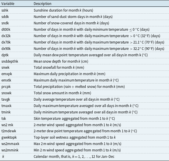

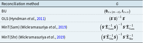
 G
G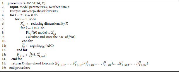
 y^T+h|T
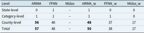

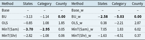
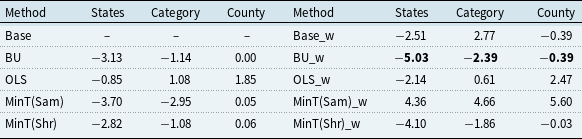
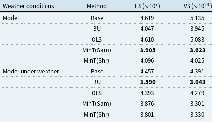

 ±50%
±50%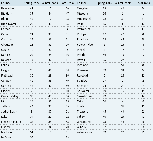
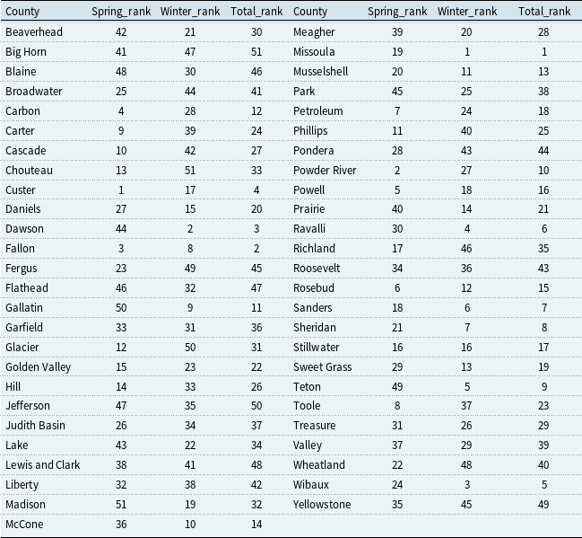
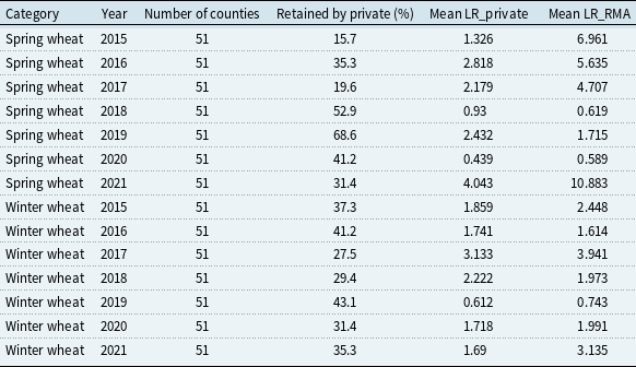
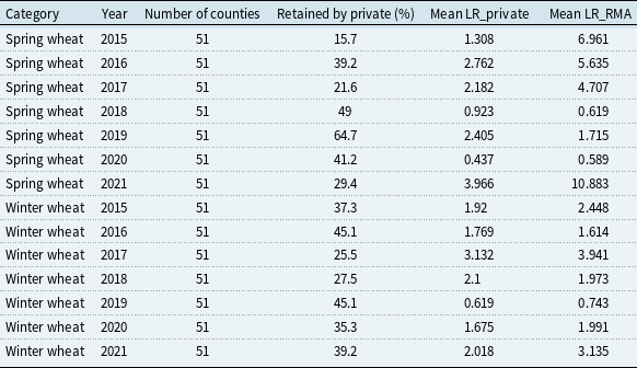


 Open access