2. Gradual onset of the awareness of continental mobility

The idea that continents have not always been fixed in their present positions and might have ‘drifted’ had been put forward three centuries before Alfred Wegener presented his theory of continental drift. The Flemish cartographer and geographer Abraham Ortelius (1527–1598) discussed Plato's Atlantis legend in the third edition of his Thesaurus Geographicus. Ortelius (Reference Ortelius1596) suggested that Plato had described an ancient separation of the continents, and used this interpretation to account for the matching coastlines of the Old and New Worlds (Romm, Reference Romm1994). He suggested that the Americas were ‘torn away from Europe and Africa . . . by earthquakes and floods’ and that ‘the vestiges of the rupture reveal themselves, if someone brings forward a map of the world and considers carefully the coasts of the three [continents]’ (Ortelius, Reference Ortelius1596). He noticed that the east coast of South America and the west coast of Africa could fit together perfectly, like a jigsaw if they were just closer, or if the Atlantic Ocean was closed. He also recognized that the continents were moving as can be seen by his statement ‘torn away from Europe and Africa . . . by earthquakes and floods’. Ortelius used for his idea a world map, which he published in 1570 in his atlas Theatrum Orbis Terrarum (Ortelius, Reference Ortelius1570). Unfortunately, Ortelius was living a few centuries too early and his innovative idea was not further explored till the 19th century.

Commonly, the credit is given to Francis Bacon (1561–1626), an English philosopher, scientist, statesman and jurist, for being the first to have observed the jigsaw fit of the opposite coasts of Africa and South America. In his book Novum Organum, published in 1620, Bacon wrote about the Old and New Worlds as examples of ‘conformable instances’ (Carozzi, Reference Carozzi1970; Romm, Reference Romm1994). This assumption, however, is evidently false, as pointed out by Davies (Reference Davies1965) and Carozzi (Reference Carozzi1970). The shape of the two continents is mentioned, but only briefly in Aphorism XXVII of Novum Organum, Lib. II. Bacon says that the Old and New Worlds both taper southwards, and that Africa and South America display a further general similarity in their outlines. It seems he did not compare the opposite coasts of the two continents, but rather noted how their west coasts were similar in outline (Davies, Reference Davies1965; Carozzi, Reference Carozzi1970). Bacon offers no discussion of the subject, but it appears that he was merely suggesting that a feature such as the ‘horn’ of East Africa may be likened to the ‘shoulder’ of Brazil, or the Gulf of Guinea to the Peru–Chile bight (Davies, Reference Davies1965).

There has been a continuing flow of ideas regarding the former geographic connection between the Old and New Worlds. In 1650, the German geographer Bernhardus Varenius (1622–1650/51?) remarked in his book Geographia Generalis that formerly America and Europe had been a single continent. He wrote that America was later torn from Europe and that the American Indians were therefore also children of Adam (Varenius, Reference Varenius1650, p. 333). The impression that Varenius (Reference Varenius1650) was probably aware of the work by Ortelius (Reference Ortelius1596) is given, but this is speculation by the authors.

Others have noted that the shapes of the continents on opposite sides of the Atlantic Ocean, most notably Africa and South America, seem to fit together. Theodor Christoph Lilienthal (1717–1781), a Königsberg Lutheran theologian, is thought to have discovered in the Bible the supposed confirmation of a break-up of the continents following Noah's flood through which the Atlantic Ocean formed. He founded his idea, among others, on the Bible verse 25 in Chapter 10 of Genesis ‘two sons were born, one was called Peleg, because in his time the earth was divided’. The most intriguing part is following: ‘Pliny testifies that formerly many countries have been separated by the sea from each other. This is also probable by the fact that the opposite coasts, though separated by the sea from each other, have a corresponding outline, so that they would almost fit together, as if they were next to each other, for example, the southern part of America and Africa’ (Lilienthal, Reference Lilienthal1756, p. 247).

Alexander von Humboldt (1769–1859), the celebrated Prussian geographer (considered one of the two founders of the modern science of geography, the other being his friend Carl Ritter), naturalist and explorer, and certainly one of the most famous scientists of this time, summarized his vast range of knowledge in the several volumes of the Kosmos: Entwurf einer physischen Weltbeschreibung (translated into English as Kosmos: A general survey of the physical phenomena of the universe). In Volume 1, he wrote ‘Our Atlantic Ocean bears every feature of a great valley. It is as if floods had directed their shocks successively to the north-east, then to the north-west, and then to the north-east again. The parallelism of the opposite coasts northward from 10° of S. latitude, their advancing and retreating angles, the convexity of the shores of Brazil opposite those of the Gulf of Guinea, the convexity of Africa under the same parallels of latitude as the deep indentation formed by the Gulf of Mexico, all vouch for this apparently bold view. In this Atlantic valley, as almost everywhere else in the configuration of great masses of land, indented and isle-studded shore stand opposite to unindented coasts. It is long since I directed attention to the circumstance how remarkable in a geological point of view was the comparison of the west coasts of Africa and South America within the tropics’ (von Humboldt, Reference von Humboldt1845a, p. 314; for the corresponding German version see von Humboldt, Reference von Humboldt1845b, p. 309; von Humboldt had first published his ideas on the comparable opposing coasts of the Atlantic in von Humboldt, Reference von Humboldt1804, pp. 404–405). Earlier, he also noted to his astonishment that orientations in the rocks of old mountain ranges in Italy, France, Switzerland, Germany and Poland are similar to those observed in the mountains in northern South America (von Humboldt, Reference von Humboldt1801, p. 333) but, as we know today, it seems he compared rocks and mountain ranges of different ages.

In 1857 Richard Owen (1810–1890), professor of chemistry and geology in Nashville, Tennessee, USA, published the idea that the entire American continent had once formed an upper layer on top of the western part of the Old World and had slid off it to open the Atlantic Ocean. He wrote ‘. . . in order to bring the hypogene rocks of America and those of northern Europe to form a regular curve . . . we must not only bring the two continents in actual contact, but we must slide a portion of North America into western Europe, the northern mass of South America on to the great Sandy Desert of Sahara, when sunk . . . beneath the waters of the ocean . . .’ (Owen, Reference Owen1857, p. 75). Owen also noted ‘The earth's crust, thus expanded and disrupted, separated, sometimes vertically, entirely through all its deposited layers, sometimes . . . by horizontal removal of an upper layer, leaving a lower layer, or vice versa: this may explain . . . various geographical peculiarities. When we restore the parts supposed disrupted . . . then we find geological formations, as well as geographical mountain-chains, etc., fitting into their original positions’ (Owen, Reference Owen1857, p. 225). Overall, Owen's observations and descriptions may be regarded as the first promising steps towards palaeogeographic reconstructions as he considered geological evidence, among other things.

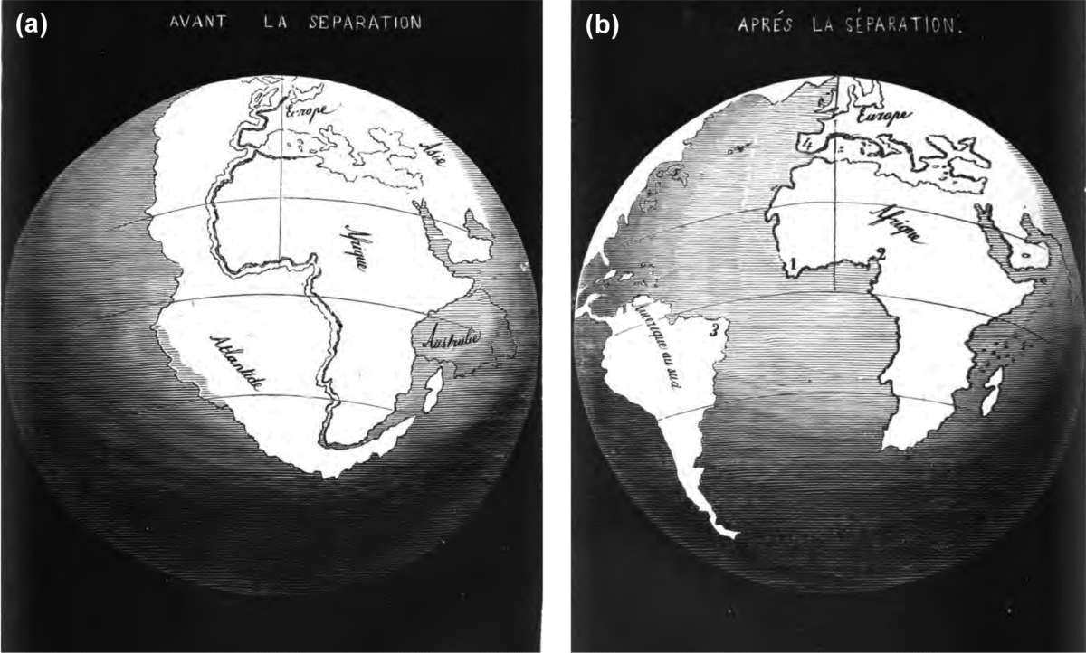
Antonio Snider-Pellegrini (1802–1885), known as Antonio Snider, a French geographer and scientist, proposed in his La création et ses mystères dévoilés (translated into English as The creation and its mysteries unveiled) that all of the continents were once connected together during late Carboniferous time (Fig. 2) and that the Atlantic had been rifted open during the Biblical Flood (Snider, Reference Snider1859, pp. 307‒315). None of the above-mentioned theories found an audience among the Earth sciences community, however.

Figure 2.

Snider (Reference Snider1859) compiled these two maps (several decades before Alfred Wegener's theory of continental drift), depicting his version of how the African and American continents may once have fit together before subsequently becoming separated: (a) assumed configuration of continents in late Carboniferous time and (b) present configuration. These maps were made famous by the publications of Carozzi (Reference Carozzi1969, Reference Carozzi1970), who reintroduced them to the geological readership in the 1970s as an early theory of continental drift.

Austrian geologist Eduard Suess (1831–1914), was, among others, an expert on the Alps. He gradually developed views on the connection between Africa and Europe and came to the conclusion that the Alps to the north were once at the bottom of an ocean, of which the Mediterranean was a remnant. He is credited with discovering the Tethys (often referred to as the Tethys Ocean), which he named in 1893 after the Titan Tethys, the daughter of Uranus and Gaia and the sister and consort of Oceanus, the ancient Greek god of the ocean (Suess, Reference Suess1893). His other major discovery was that the Glossopteris flora ‒ an extinct group of seed ferns that arose during Permian time but became extinct by the end of the Triassic Period ‒ were found in South America, Africa, India and Australia. His explanation was that the three lands were once connected into a supercontinent, which he named originally Gondwana-Land (proposed in 1885) (from the Sanskrit gondavana meaning ‘forested (land) of the Gonds’), a historic region in central India. Note that the name Gondwana had already been introduced into geological vocabulary in 1872 by the Irish geologist Henry Benedict Medlicott (1829‒1905) who served as Director of Geological Survey of India from 1876 to 1887 (see Leviton & Aldrich, Reference Leviton and Aldrich2012). The name was used for the stratigraphic Gondwana system of India (Medlicott & Blandford, Reference Medlicott and Blandford1879). Eduard Suess believed that the oceans flooded the spaces currently between those lands when the pieces in between sank. He published a comprehensive synthesis of his ideas in three volumes in five parts (Suess, Reference Suess1883, Reference Suess1885, Reference Suess1888, Reference Suess1901, Reference Suess1909) entitled Das Antlitz der Erde (translated into English as The Face of the Earth), one of the most fundamental texts of modern geology. Suess also coined the terms Laurentia, Caledonian Mountains, Variscan Mountains, Panthalassa, biosphere, lithosphere, hydrosphere, eustasy, foreland, hinterland, listric fault, horst and graben, today part of the established Earth sciences vocabulary and closely connected with plate tectonics and palaeogeography (see Şengör, Reference Şengör2014a, Reference Şengör2015).

3. The rise of the theory of continental drift

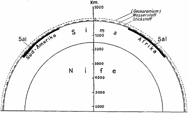
It was not until 1912 that the idea of lateral mobility of continents was seriously considered – at least by a few masterminds – as a scientific theory called ‘Kontinentalverschiebung’ (as written in the original version), translated into English as ‘continental drift’. The German meteorologist Alfred Wegener (1880–1930) presented his theory to the public for the first time in a lecture entitled Die Heraushebung der Großformen der Erdrinde (Kontinente und Ozeane) auf geophysikalischer Grundlage (translated into English as The uprising of large features of earth's crust (Continents and Oceans) on geophysical basis) at the annual general meeting of the Geologische Vereinigung on 6 January 1912 in Frankfurt am Main (Wegener, Reference Wegener1912a, Reference Wegenerb) in the Senckenberg Museum lecture hall (where a plaque to that effect now hangs). Wegener suggested that continents were joined together at one time. Thereafter, they moved through the Earth's simatic crust like ice-breakers ploughing through sea ice, finally reaching their present position. His theory centred around the hypothesis that the continents consist of a lighter assemblage of elements called Sal – an acronym of silicon and aluminium, introduced by Eduard Suess in the last volume of Das Antlitz der Erde – which isostatically float on a heavier assemblage of elements of the Earth's outer mantle called Sima – an acronym of silicon and magnesium (Fig. 3); today, Sal is called sial.

Figure 3.

Schematic view of a section of the Earth's surface to its core indicating that the continents (Sal) float on the outer viscous crust (Sima), according to Alfred Wegener's model of continental drift (Wegener, Reference Wegener1912a, p. 279).

Frankly speaking, much of what he proposed was not completely new because he based his idea on earlier observations and suggestions. It was however topped by a broad array of newly collected evidence, and his theory initiated a lively discussion among scientists. For example, he wrote ‘The first concept of continental drift first came to me as far back as 1910, when considering the map of the world, under the direct impression produced by the congruence of the coastlines on either side of the Atlantic. At first I did not pay attention to the idea because I regarded it as improbable. In the fall of 1911, I came quite accidentally upon a synoptic report in which I learned for the first time of palaeontological evidence for a former land bridge between Brazil and Africa. As a result, I undertook a cursory examination of relevant research in the fields of geology and palaeontology, and this provided immediately such weighty corroboration that a conviction of fundamental soundness of the idea took root in my mind’ (Wegener, Reference Wegener1929, p. 1; for the English translation see Wegener, Reference Wegener1966, p. 1). He published the core idea of ‘continental drift’ first in two papers (Wegener, Reference Wegener1912a, Reference Wegenerb) and then in the first edition of his book Die Entstehung der Kontinente und Ozeane (translated into English as The Origin of Continents and Oceans) (Wegener, Reference Wegener1915), followed by three revised editions (Wegener, Reference Wegener1920, Reference Wegener1922 and Reference Wegener1929) which each contained new data.

One of the basic concepts that helped Wegener document the continental drift was the idea of a large united landmass consisting of most of the Earth's continental regions. In his theory, Wegener introduced the supercontinent of Pangaea (derived from πᾶν-γαῖα, Greek for ‘all earth’) to explain the ancient climate similarities, fossil evidence and similarity of rock structures between Africa and South America, as well as the outlines of the continents, especially the continental shelves, which seem to fit together (Fig. 4). Wegener used the following geological evidence, among others, to support his theory. (1) Similar rock types were found in mountain ranges on either side of the Atlantic Ocean, for example the Appalachian Mountains of northeastern North Americas linked to the Scottish Highlands and those south of New York to the Hercynides of France and Spain. (2) Similar (or closely related) fossils were found on either side of the Atlantic Ocean, implying that the continents were once joined together. (3) Fossil tropical land plants were found in rocks which are now in the polar regions; in 1912, Glossopteris was found in Antarctica (e.g. Osborne, Royer & Beerling, Reference Osborne, Royer and Beerling2004) during the famous and ill-fated Terra Nova Expedition (British Antarctic Expedition between 1910 and 1913) with the British Royal Navy officer and explorer Captain Robert Falcon Scott (1868‒1912) as its leader.

Figure 4.

Alfred Wegener's palaeogeographic reconstructions of the world for three periods (late Carboniferous, Eocene and older Quaternary) according to the theory of continental drift (from Wegener, Reference Wegener1929, fig. 4). The upper map shows the supercontinent of Pangaea. Shaded, ocean; dotted, shallow sea; latitude and longitude arbitrary.

Wegener's theory of continental drift was either ignored or downright ridiculed by the scientific community (e.g. Soergel, Reference Soergel1916; Andrée, Reference Andrée1917; Kossmat, Reference Kossmat1921; Penck, Reference Penck1921; Schweydar, Reference Schweydar1921; Jaworski, Reference Jaworski1922; Nölke, Reference Nölke1922). The Americans were particularly adamant; Bailey Willis (Reference Willis1944) called Wegener's theory ‘ein Märchen’ (a fairy tale) and Oreskes (Reference Oreskes1999) provided several reasons for the American rejection. First, Wegener was not a geologist by profession, which of course was most welcome by his opponents. Secondly, most influential geoscientists at that time were based in the Northern Hemisphere, whereas most of the conclusive data came from the Southern Hemisphere. Thirdly, Wegener thought that Pangaea did not break up until Cainozoic time, and palaeontologists found it hard to believe that so much continental drift could have occurred in so short a time. Last but not least, the greatest problem remained the lack of direct evidence for the movements of continents and the needed explanation for the mechanism. Wegener thought the force of Earth's spin was sufficient to cause continents to move, but geophysicists knew that rocks are too strong for this to be true. Wegener also thought that the continents were moving through the Earth's simatic crust, like ice-breakers ploughing through sea ice (Fig. 3). Geologists noted that ploughing through oceanic crust would distort continents beyond recognition, and geophysicists could not think of a force strong enough to make continents able to plough through oceanic crust. Consequently, Wegener's theory of continental drift is in many aspects erroneous because it is not the individual continents which move, but the entire plates of the lithosphere, and the driving forces of slab pull and ridge push (Forsyth & Uyeda, Reference Forsyth and Uyeda1975) come from within the Earth. The movement of plates is not driven by the rotation of the Earth. Wegener's theory was heavily attacked by most of the Earth scientists of this time. Wegener was unable to obtain a regular professorship at any of the universities or technical high schools in Germany because he was ‘interested also, and perhaps to a greater degree, in matters that lay outside its terms of reference’ (Horvitz, Reference Horvitz2002, p. 162). The University of Graz in Austria was more tolerant of controversy and, in 1924, appointed him professor of meteorology and geophysics. Regardless of the controversies mentioned above, perhaps Wegener's most important legacy is to have introduced the idea of lateral mobility of continents, that is, offering a paradigm change from fixism to mobilism to the scientific community and the public. Overwhelmingly however, most of the established geologists were convinced that the Earth's continents were immobile and neglected Wegener's foresighted approach.

One of Wegener's staunchest supporters was the South African geologist Alexander Logie du Toit (1878–1948); Reginald Aldworth Daly considered him the greatest field geologist of the 20th century. In 1923, du Toit was awarded a Carnegie Institute grant to travel to South America to test his thesis that rock formations in South Africa have their counterparts in Brazil. They indeed do, convincing him that African and South American continents had once been joined and have drifted apart (Fig. 5). He published his observations in the Publication of the Carnegie Institution of Washington entitled A Geological Comparison of South America with South Africa (du Toit, Reference du Toit1927; a slightly expanded version in Portuguese was published posthumously in 1952 in Brazil, du Toit, Reference du Toit1952), and later he developed his ideas in Our Wandering Continents: An Hypothesis of Continental Drifting (du Toit, Reference du Toit1937). du Toit (Reference du Toit1937) proposed that Wegener's Pangaea first broke into two large continental landmasses: Laurasia in the Northern Hemisphere and Gondwana-Land (which du Toit inappropriately shortened to Gondwana) in the Southern Hemisphere. Laurasia and Gondwana-Land then continued to break apart into the various smaller continents that exist today.

Figure 5.

Reconstruction of Gondwana for the Palaeozoic Era according to du Toit (Reference du Toit1937, fig. 7). The space between the various portions was then mostly land. Short lines indicate the pre-Cambrian or early Cambrian grain. Stippling marks out regions of late Cretaceous and Tertiary compression. Later, Smith & Hallam (Reference Smith and Hallam1970) presented a computer fit of the contour of the southern continents forming Gondwana-Land.

Another strong supporter of Wegener's theory of continental drift was Boris Choubert (1906–1983), a French geologist of Russian origin. He was the first scientist to present a very accurate geometrical fit of the circum-Atlantic continents using continental edges instead of coastlines (Choubert, Reference Choubert1935) (Fig. 6a); this was remarkably like the oft-cited ‘Bullard fit’ reconstructed 30 years later (Fig. 6b), further demonstrating that the continents were closely jointed together at one time. Choubert interpreted the Precambrian and the Palaeozoic (‘Caledonian’ and ‘Hercynian’) belts as the result of horizontal movements of the Precambrian blocks. This pioneer was however overlooked for many years, as pointed out by van Houten (Reference van Houten1975). Kornprobst (Reference Kornprobst2017) analysed the lack of recognition of Choubert's work and came to the conclusion that it was related to a great evolution in the geological concepts between 1935 and 1965, and the poor choice of Choubert regarding the title of his 1935 publication. Some scientists have been aware of this unfairness in the recognition of Choubert's work. At a scientific meeting at the beginning of the 1970s, the French geophysicist Xavier Le Pichon, one of the pioneers of plate tectonics, proposed that the circum-Atlantic continents fit should be called the ‘Bullard–Choubert fit’ (Kornprobst, Reference Kornprobst2017, p. 48). Although this proposal was not further considered by the scientific community, it should be on the agenda of forthcoming international scientific meetings as the great work of Boris Choubert should be honoured in some way. Choubert's geological and palaeogeographical work was also analysed by Şengör (Reference Şengör2014b) and Letsch (Reference Letsch2017), and highlights once more Choubert's masterpieces of Earth sciences research before the emergence of the theory of plate tectonics.

Figure 6.

Pre-Permian (‘Hercynian’) palaeogeographic reconstructions for the assemblage of the circum-Atlantic continents. (a) Reconstruction based on a composite bathymetric map of the Atlantic Ocean, choosing the continental edge instead of the coastline as the relevant continental boundaries (Choubert, Reference Choubert1935, fig. 2). Choubert (Reference Choubert1981) provides some information on how he worked out his 1935 reconstruction. (b) Reconstruction achieved by fitting of the continental margins at the 500 fathom line (approximately 900 m) as a proxy for the edge of the continental shelf (Bullard et al. Reference Bullard, Everett and Smith1965, fig. 8). Red, overlaps; blue, gaps. The so-called ‘Bullard fit’ described the first use of numerical methods to generate a computerized fit of the continents. Reprinted from Bullard, E., Everett, J. E. & Smith A. G. 1965, The fit of the continents around the Atlantic, Philosophical Transactions of the Royal Society of London, Series A, Mathematical and Physical Sciences 258, 41−51, by permission of the Royal Society.

Reginald Aldworth Daly (1871–1957), a Canadian igneous petrologist and a highly regarded geology professor at Harvard University, was also a proponent of Wegener's theory. Daly expressed his support by putting E pur si muove! (translated into English as And yet, it moves!) on the title page of his book Our Mobile Earth (Daly, Reference Daly1926).

4. Transition from continental drift to plate tectonics

Wegener's theory of continental drift (Wegener, Reference Wegener1912a, Reference Wegenerb, Reference Wegener1915) became the spark that ignited a new way of viewing the Earth that led some scientists to start searching for an explanation of how continents could move. Robert Schwinner (1878–1953), an Austrian geologist and geophysicist, had revived an old idea of von Humboldt's that convective magma flows might exist in the mantle and that the continents are riding on the back of those slow convective current streams (Schwinner, Reference Schwinner1920, Reference Schwinner1941). The Austrian geologist Otto Ampferer (1875–1947) had a similar idea, and probably presented the first model of convection currents being responsible for continental drift (Ampferer, Reference Ampferer1925) (Fig. 7). As early as in 1916 and later in 1928 the Dutch geologist Gustaaf Adolf Frederik Molengraaf (1860–1942) identified the mid-Atlantic ridge as a volcanic structure, and argued that a locus of ocean-floor spreading was separating the continents on both sides of the Atlantic (see Molengraaf, Reference Molengraaf1916, Reference Molengraaf, van Waterschoot van der Gracht, Willis, Chamberlin, Joly, Molengraaff, Gregory, Wegener, Schuchert, Longwell, Taylor, Bowie, White, Singewald and Berry1928). Ampferer followed his lead in a remarkable paper in 1941 entitled Gedanken über das Bewegungsbild des atlantischen Raumes (Ampferer, Reference Ampferer1941; see also Thenius, Reference Thenius1988). Likewise, Arthur Holmes (1890–1965), a British geologist who early on realized the great potential of Lord Rutherford's discovery in 1911 that radioactivity provided a means to measure the ages of minerals (Holmes, Reference Holmes1913, Reference Holmes1946), came up with an explanation for why continents could move, but it was more advanced than the theories of Schwinner and Ampferer. Holmes suggested that heat trapped in the Earth's mantle caused vast, slow-moving convection currents and that this was the power source that Wegener needed to make the continents drift (e.g. Holmes, Reference Holmes1928, Reference Holmes1931, Reference Holmes1944). In the famous first edition of his book Principles of Physical Geology, he shows a drawing of mantle convection and wrote ‘Currents flowing horizontally beneath the crust would inevitably carry the continents along with them’ (Holmes, Reference Holmes1944, p. 506). He also suggested ‘. . . the currents . . . drag the two halves of the original continent apart, with consequent mountain building in front where the currents are descending, and ocean floor development on the site of the gap, where the currents are ascending’ (Holmes, Reference Holmes1944, p. 506). The last statement refers to mid-ocean ridges; their discovery was another milestone in Earth sciences that contributed towards the theory of plate tectonics, which steadily replaced the theory of continental drift. But when, how and by whom was the discovery of mid-ocean ridges made?

Figure 7.

Schematic model showing convection currents being responsible for continental drift (Ampferer, Reference Ampferer1925, his fig. 6). Translation of the German words: Kontinentalscholle, continent; aufsteigende Strömung, ascending current; absteigende Strömung, descending current; Antrieb von innen, drive from the inside.

In 1850 Matthew Fontaine Maury (1806–1873), a US Navy lieutenant and an expert of the sea (thus nicknamed ‘Pathfinder of the sea’), inferred a ridge in the middle of the Atlantic Ocean while evaluating acoustic soundings acquired with the research vessel Dolphin. He presented his findings in The Physical Geography of the Sea (Maury, Reference Maury1855). A few decades later, the British vessel HMS Challenger (1872–1876) set off to explore the Atlantic Ocean. The first bathymetric chart of the entire Atlantic Ocean by Murray & Renard (Reference Murray and Renard1891), synthesized from bathymetric data acquired during the HMS Challenger expedition, reveals a structure in the middle of the ocean which can be interpreted as a ridge. The sparse acoustic soundings only permitted generalized contours, however; a more detailed outline of the ridge and the ocean floor was still to be made. For that, we shall now move to Germany.

The German chemist Fritz Haber (1868–1934), who was awarded the Nobel Prize in Chemistry in 1918 (received in 1919), suggested that Germany could ease its war debts after World War I by extracting gold from seawater (Mero, Reference Mero1965, p. 41). This suggestion was based on the assumption that gold was in seawater in concentrations of 5‒10 mg of gold per ton of seawater (Haber, Reference Haber1927, p. 303). Haber was therefore secretly assigned to extract gold from the sea, ‘a dream of generations of scientists’ (Broad, Reference Broad1997, p. 252). In 1925, the legendary German research vessel Meteor set out in great secrecy to systematically explore the Atlantic Ocean from the Antarctic region to the tropics of the North Atlantic. Huge volumes of seawater were examined for information on water chemistry and temperature, and some 67000 acoustic soundings were conducted. After two years of study, they returned with the data. Haber found that the sample from the Meteor's cruise had a mean gold content of 0.008 mg of gold per ton of seawater (Haber, Reference Haber1927, p. 310); he therefore failed as there is much less gold in seawater than earlier assumed. However, the expedition identified in great detail a long ridge running along the middle of the Atlantic Ocean as illustrated on the first detailed bathymetric chart of the South Atlantic (Maurer & Stocks, Reference Maurer and Stocks1933), which was incorporated into the Atlantic bathymetric map of the time by Stocks & Wüst (Reference Stocks and Wüst1935). The identified ridge later became known as the Mid-Atlantic Ridge (Heezen, Tharp & Ewing, Reference Heezen, Tharp and Ewing1959). It is a mid-ocean ridge, that is, a mountain range on the floor of the Earth's oceans, an important key to the theory of plate tectonics.

Much was speculated about the origin of the mid-ocean ridges until the American geologist Harry Hess (1906–1969), who conducted extensive sea-floor mapping during World War II, published a ground-breaking paper entitled History of Ocean Basins (Hess, Reference Hess, Engel, James and Leonard1962) in which he developed his idea of sea-floor spreading, a forerunner of plate tectonics. He reinvented Molengraaf's idea that the sea floor forms at the mid-ocean ridge and moves horizontally from the ridge crest towards an oceanic trench, where it is subducted into the mantle. Convection in the mantle is the driving force for this process. One year earlier, Dietz (Reference Dietz1961) had proposed a concept referred to ‘spreading sea-floor theory’; his argumentation was not necessarily independent however (as Hess’ manuscript had been circulating in scientific circles since 1959), and was not as detailed as that by Hess (Reference Hess, Engel, James and Leonard1962). From the 1950s onwards the world's oceans were extensively investigated with magnetometers, among others. Magnetic anomalies arranged in linear patterns on the seafloor subparallel with respect to the ocean-spreading ridges were identified, first on the sea floor off California (Mason, Reference Mason1958; Mason & Raff, Reference Mason and Raff1961) and later in other ocean basins. Lawrence Morley (his paper was rejected by Nature) and Vine & Matthews (Reference Vine and Matthews1963) were the first to recognize their importance and present an explanation for these linear pattern, which developed due to numerous reversals in the Earth's magnetic field. Each magnetic stripe was magnetized when that piece of ocean floor was formed in the central valley on the mid-ocean ridge axis.

In the light of these new discoveries, a better understanding of how the Earth seems to work was on its way. Some scientists were however sceptical with the convection current hypothesis as the main driver of sea-floor spreading, and instead favoured a general expansion of the Earth (e.g. Heezen & Tharp, Reference Heezen and Tharp1965; Oppenheim, Reference Oppenheim1967). Nevertheless, a re-evaluation of Wegener's theory of continental drift, the movements of the continents and their arrangements through geological time became once more a topic of interest among the scientific community (e.g. Carey Reference Carey1955, Reference Carey and Carey1958).

The first computational approach in palaeogeography was presented by Sir Edward Bullard (1907–1980), Jim E. Everett and Alan G. Smith (1937–2017) in their famous paper ‘The fit of the continents around the Atlantic’ (Bullard, Everett & Smith, Reference Bullard, Everett and Smith1965), which shows a very accurate geometrical fit of the circum-Atlantic continents using the early Cambridge University EDSAC 2 computer. They used the real ‘edge of the continent’, that is, the continental margin instead of the coastlines (Fig. 6b). This fit became known as the ‘Bullard fit’ (Bullard, Reference Bullard1969), although much of the work was done by the co-authors (Bullard, Reference Bullard1975, p. 21). Although they were concerned only with the kinematic approach and were not discussing the mechanism by which continents split and oceans formed, the paper by Bullard, Everett & Smith (Reference Bullard, Everett and Smith1965) can be seen as a linking transition between the theories of continental drift and plate tectonics (Dewey, Reference Dewey2015). With the immense knowledge gained in the 1950s and early 1960s, including Wilson's ‘hot spots’ hypothesis (Wilson, Reference Wilson1963), all foundation stones for the forthcoming plate tectonics theory had been laid out.

5. Flourishing of the plate tectonics paradigm

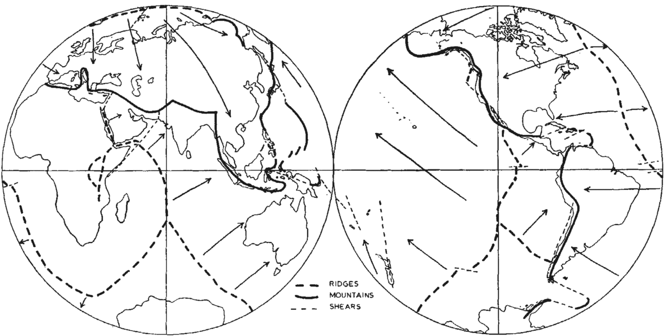
The plate tectonics theory celebrated its semi-centennial in 2015. It was introduced by the Canadian geophysicist and geologist John Tuzo Wilson (1908–1993) in a ground-breaking paper in Nature in 1965, in which he defined the nature of the plates and plate boundaries and discussed the continuous motion of rigid plates with respect to one another (Wilson, Reference Wilson1965) (Fig. 8). Unknowingly following Argand (Reference Argand1924), Wilson (Reference Wilson1966) suggested the existence of a proto-Atlantic Ocean prior to the late Palaeozoic assembly of the Pangaea, and that the ocean must have closed before Carboniferous time and later re-opened to form the present-day Atlantic Ocean (such repeated opening and closing of an ocean basin came to be known as the ‘Wilson Cycle’, a term coined by Kevin Burke in Burke & Dewey, Reference Burke and Dewey1973). The papers of McKenzie & Parker (Reference McKenzie and Parker1967), Sykes (Reference Sykes1967), Morgan (Reference Morgan1968), Le Pichon (Reference Le Pichon1968) and Isacks, Oliver & Sykes (Reference Isacks, Oliver and Sykes1968) were seminal in providing diverse tests of the theory and their successful tests helped to establish it as the unifying theory of tectonics. The motions of the rigid plates were described as rotations across Earth's spherical surface by defining poles, known as Euler poles. Publications on plate tectonics flourished in the following years (e.g. Dewey, Reference Dewey1969a, Reference Deweyb; Hamilton, Reference Hamilton1969, Reference Hamilton1970; Laubscher, Reference Laubscher1969; Mitchell & Reading, Reference Mitchell and Reading1969; Bird & Dewey, Reference Bird and Dewey1970; Dewey & Bird, Reference Dewey and Bird1970a, Reference Dewey and Birdb, Reference Dewey and Bird1971; Dickinson, Reference Dickinson1971a, Reference Dickinsonb; Wilson, Reference Wilson1972; Marvin, Reference Marvin1973; Tarling & Runcorn, Reference Tarling and Runcorn1973; Dewey, Reference Dewey1975; Cox & Hart, Reference Cox and Hart1986; Davies, Reference Davies1992). By the early 1970s, the term ‘plate tectonics’ was well established in the Earth sciences vocabulary. Today, the Earth's lithosphere is divided into seven large and a few smaller plates. The plates move slowly at a rate of a few centimetres per year and change size. Plates may be entirely made up of continental rocks, both continental and oceanic rocks, or entirely of oceanic rocks. Continental plates on Earth appear to have a tendency to episodically assemble, disperse and re-assemble in various supercontinental configurations (e.g. Dewey, Reference Dewey, Aufley-Charles and Hallam1988; Nance, Murphy & Santosh, Reference Nance, Murphy and Santosh2014), although these peculiarities are still under debate (e.g. Bradley, Reference Bradley2011).

Figure 8.

John Tuzo Wilson's sketch maps illustrating the present network of mobile belts, comprising the active primary mountains and island arcs in compression (solid lines), active transform faults in horizontal shear (light dashed lines) and active mid-ocean ridges in tension (bold dashed lines) (Wilson, Reference Wilson1965, fig. 1). Reprinted by permission from Macmillan Publishers Ltd: Nature. Wilson J. T., A new class of faults and their bearing on continental drift. Nature 207, 343–347 (1965), copyright 1965.

Following Hutton's ‘Principle of Uniformity’, plate tectonics must be ongoing for at least three billion years, if not more. However, the onset of plate tectonics is still a hot topic of scientific discussion and a few comprehensive reviews have already been written (e.g. Condie & Pease, Reference Condie and Pease2008). Some believe that the onset of modern-style plate tectonics on Earth began in the Neoproterozoic Period, documented by the first appearance of high-pressure, low-temperature rocks such as oceanic blueschists and low-temperature eclogites, and ultrahigh-pressure intracontinental complexes and kimberlite diatremes (Stern, Reference Stern2005; Stern, Leybourne & Tsujimori, Reference Stern, Leybourne and Tsujimori2016). There is, however, a growing consensus that plate tectonics in general started much earlier (see de Wit & Ashwal, Reference De Wit and Ashwal1997; Harrison et al. Reference Harrison, Blıchert-Toft, Müller, Albarede, Holden and Mojzsis2005; Cawood, Kröner & Pisarevsky Reference Cawood, Kröner and Pisarevsky2006; Polat, Kerrich & Windley, Reference Polat, Kerrich, Windley, Cawood and Kröner2009; Korenaga, Reference Korenaga2013). During 3–2 Ga the Earth record shows some fundamental geological and geochemical changes, which may be an expression of the cooling of the Earth's mantle and corresponding changes in convective style and the strength of the lithosphere, and they may record the gradual onset and propagation of plate tectonics (Condie, Reference Condie2016). Based on hafnium isotopes (Harrison et al. Reference Harrison, Blıchert-Toft, Müller, Albarede, Holden and Mojzsis2005) and data from experimental petrology (Hastie et al. Reference Hastie, Fitton, Bromiley, Butler and Odling2016), it is suggested that the first continents had formed at c. 4 Ga and that subduction processes were also active. Primitive plate tectonics (‘permobile regime’: Burke, Dewey & Kidd Reference Burke, Dewey, Kidd and Windley1976) may have started in the Hadean Period soon after the magma ocean solidified (Ernst, Sleep & Tsujimori Reference Ernst, Sleep and Tsujimori2016; Ernst, Reference Ernst2017), but that is under debate (e.g. Stern, Leybourne & Tsujimori, Reference Stern, Leybourne and Tsujimori2017). Regardless of these controversies, plate tectonics has been ongoing for a long period of time, changing the face of the Earth and thus providing the working base for studying Earth's palaeogeography.

6. Palaeogeographic studies before plate tectonics

Most of the palaeogeographic work before the rise of plate tectonics was centred on the description of the rock record, including its fossil content, and was confined to showing the distribution of lands and seas on modern base maps. In the early days, the presentation of palaeogeography simply meant illustrating palaeofacies changes through time. To the authors’ knowledge, the earliest scientific palaeogeographic map is by the French naturalist Jean Honoré Robert de Paul de Lamanon, known as Robert de Lamanon (1752–1787). De Lamanon (Reference de Lamanon and de1782) studied some vertebrate fossils from the gypsum quarries of Montmartre in Paris, and decided that the gypsum was deposited in lakes and not in the sea on the basis of the fossils he considered. He then established the horizontal limits of the gypsum, which he assumed had been those of the former lake. Figure 9 shows his palaeogeographical map of Montmartre at the time of the existence of the lake. De Lamanon had no means of dating his lake. He only knew that some of the animals that lived in it no longer existed, and thus the lake must have existed before the present fauna was established.

Figure 9.

Robert de Lamanon's map of Montmartre (central part of the Paris Basin) at the time of the existence of the lake (de Lamanon, Reference de Lamanon and de1782). To the authors’ knowledge, this is the earliest palaeogeographical map.

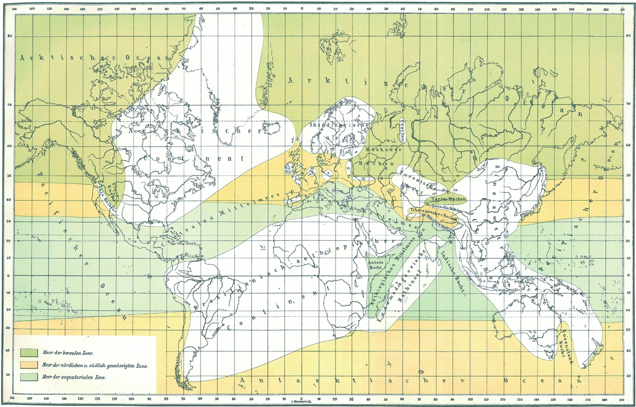
In the middle of the 19th century, palaeogeographical studies advanced as shown by the publications of de Beaumont (Reference de Beaumont1833), Lyell (Reference Lyell1835), Beudant (Reference Beudant, Beudant, Milne-Edwards and de Jussieu1841), Marcou (1857–Reference Marcou1860) and Dana (Reference Dana1863). The famous map of Neumayr (Reference Neumayr1885) showing the geography of the Jurassic Period (Fig. 10) is the most detailed palaeogeographic map of the entire Earth published during the 19th century. In that map, we see not only the distribution of land and sea during the Jurassic Period but also the extent of what Melchior Neumayr (1845–1890), a German palaeontologist from Munich who spent much of his professional life in Vienna working closely with his father-in-law Eduard Suess, called the ‘sea of the boreal zone’, the ‘sea of the temperate zone’ and the ‘sea of the equatorial zone’, indicating the Jurassic climatic zones by the distribution of climate-sensitive rock assemblages and fossils.

Figure 10.

Melchior Neumayr's famous map showing the geography of the Jurassic Period (Neumayr, Reference Neumayr1885, plate I) is the most detailed palaeogeographic map of the entire Earth published during the 19th century. Translation of the legend: Meer der borealen Zone, sea of the boreal zone; Meer der nördlichen u. südlich gemässigten Zone, sea of the northern and the southern temperate zone; Meer der aequatorialen Zone, sea of the equatorial zone. White indicates land areas and the coloured regions are the seas.

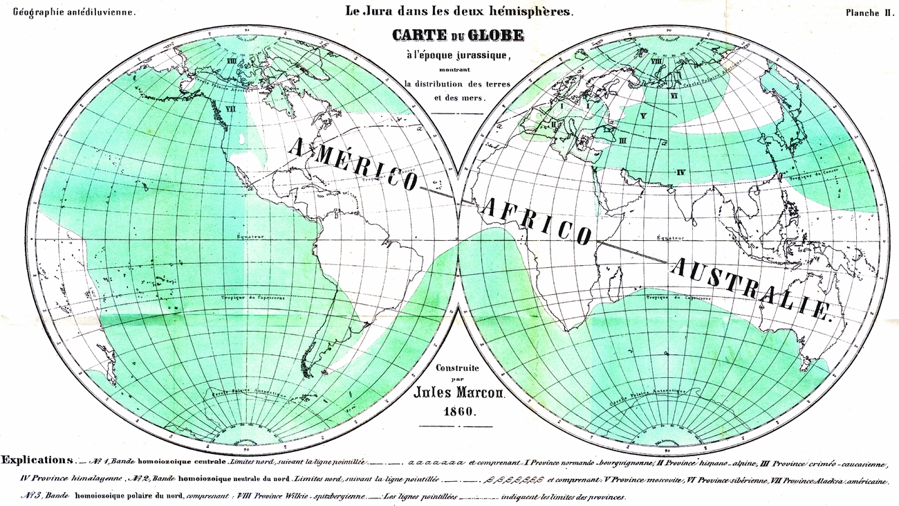
The first global palaeogeographical map was not however by Neumayr, but by the French geologist Jules Marcou (1824–1898); Marcou also published a map of the Jurassic Period of the entire world in 1860 (Fig. 11). It was much more primitive than Neumayr's, but it was a pioneer attempt. The classical work of Suess (Reference Suess1883, Reference Suess1885, Reference Suess1888, Reference Suess1901, Reference Suess1909) is well known, but Suess produced no palaeogeographic map, confining his descriptions to texts. Other publications worth mentioning are comprehensive works by Koken (Reference Koken1893), Canu (Reference Canu1895) and de Lapparent (Reference de Lapparent1900), just to name a few.

Figure 11.

Jules Marcou's reconstruction of the palaeogeography of the Jurassic Period showing the distribution of oceans and continents and biogeographic provinces (Marcou, 1857‒Reference Marcou1860, foldout plate II). Blue shows the seas and white the lands. The explanations hardly need a translation except for pointillie (dotted) and suivant (following).

The greatest development of palaeogeographic maps took place during the 20th century, with the previously unimaginable development in the precision of dating rocks and improvement in our knowledge of regional geology including the bottoms of the oceans. Palaeogeography became in vogue among Earth scientists during the first quarter of the 20th century, as shown by the increased number of publications at this time. Willis (Reference Willis1910, p. 241) appropriately noted that palaeogeography ‘is a young science that has all its future before it’. Most of the published maps focused on a specific area and certain time slice and, of course, were still following the ‘fixist’ view (e.g. Matthew, Reference Matthew1906). Theodor Arldt (1878–1960), a German natural scientist, historian and secondary school teacher, presented a collection of palaeogeographic maps from the Cambrian to the Recent periods in his book entitled Die Entwicklung der Kontinente und ihrer Lebewelt (translated into English as The Evolution of Continents and Their Living World) (Arldt, Reference Arldt1907; second edition 1938, of which only the first volume was published (Arldt, Reference Arldt1938) because the manuscript of the second volume was destroyed during World War II) (Fig. 12). Toula (Reference Toula1908) presented a thorough discussion about this new approach in palaeogeography. A few years later, Arldt discussed the changing size of continents and oceans and the depths of the ocean basins through time, as well as mountain belts and their relation to the continental margins (Arldt, Reference Arldt1912). In 1914, Arldt provided a first review of palaeogeographical reconstructions (Arldt, Reference Arldt1914). He summarized his vast range of knowledge in two volumes of the Handbuch der Palaeogeographie (Arldt, 1917–Reference Arldt1922) to which we refer, as it contains many references and provides a comprehensive overview of the knowledge from this time. Edgar Dacqué (1878–1945), a German geologist and palaeontologist, also spent much time with palaeogeographic research and summarized his ideas in a number of publications (e.g. Dacqué, Reference Dacqué1913) and comprehensive text books such as Grundlagen und Methoden der Paläogeographie (translated into English as Basics and Methods of Palaeogeography) (Dacqué, Reference Dacqué1915) and Geographie der Vorwelt (Paläogeographie) (translated into English as Geography of the Past (Palaeogeography)) (Dacqué, Reference Dacqué1919). In the Encylopaedia of Geography published by Deuticke in Vienna, Dacqué and Wegener published a volume together under the title Paleogeographie, each writing a section (Dacqué, Reference Dacqué1926).

Figure 12.

Palaeogeographic map for the Cretaceous Period reproduced from Arldt (Reference Arldt1907).

The Austrian–German geologist Franz Kossmat (1871–1938) was the first to publish a popular book for the general public simply entitled Paläogeographie (Kossmat, Reference Kossmat1908) which went through three editions, the last being in 1924. In his book, he gives an outline of Earth history from the Cambrian Period to the ‘Diluvium’, supplemented by palaeogeographic maps showing the distribution of lands and seas during the Silurian (Fig. 13), Devonian, Carboniferous, Triassic, Cretaceous and Old-Tertiary periods. Note that the term ‘Diluvium’ was introduced into literature in 1823 by the English theologian William Buckland (1784–1856) in his classic book Reliquiae Diluvianae (Buckland, Reference Buckland1823) for the youngest deposits on Earth, considered a product of the Biblical Flood (the ‘Diluvial Theory’). Forbes (Reference Forbes1846) proposed equating the term ‘Pleistocene’ – introduced by Lyell (Reference Lyell1839, p. 616–621) and commonly referred to as the ‘Glacial Epoch’ – with the Diluvium. Worth mentioning is also another book by Kossmat related to palaeogeography, entitled Paläogeographie und Tektonik (Kossmat, Reference Kossmat1936), in which a comprehensive overview of the relation between palaeogeography and the tectonic structure of the Earth's surface is provided. Different regions of the globe are discussed from the Archean to the Quaternary eras, supplemented by palaeogeographic maps showing the distribution of land and seas in the Cambrian, Devonian, early Carboniferous (Viséan), late Carboniferous, Triassic, Late Cretaceous and middle Eocene periods.

Figure 13.

Palaeogeographic map for the Silurian Period reproduced from Kossmat (Reference Kossmat1908).

Grabau (Reference Grabau1909) presented palaeogeographic maps for North America for the Ordovician, Silurian and Early Devonian periods, and some trans-Atlantic palaeogeographic maps for the early Palaeozoic, which he communicated to the public during the 11th International Geological Congress in Stockholm in 1910 (Grabau, Reference Grabau1912). Willis (Reference Willis1909) also presented palaeogeographic maps for North America (12 time slices). They are too schematic however (Fig. 14), as ‘they embrace too much time, and hence do not bring out the oscillatory nature of the continental seas’ (Schuchert, Reference Schuchert1910, p. 435). Schuchert (Reference Schuchert1910), an accomplished American palaeontologist and stratigrapher of German descent (he was born in Ohio to German immigrant parents and his mother tongue was German, which enabled him to read with facility the classic geological publications in German), published the first comprehensive review of the palaeogeography of North America, presenting palaeogeographic maps for 50 time slices showing the distribution of continental and marine facies (Fig. 15); a compendium of revised maps was present later (Schuchert, Reference Schuchert1955). Discussing the use of fossils for palaeogeographic and palaeoenvironmental reconstructions such as palaeobathymetry was common practice in the early days of palaeogeographic research (e.g. Schuchert, Reference Schuchert1911).

Figure 14.

Palaeogeographic map of North America for the Silurian reproduced from Willis (Reference Willis1909).

Figure 15.

Palaeogeographic map of North America for the Middle Silurian reproduced from Schuchert (Reference Schuchert1910). The legend to the left explains the facies presented on the map.

With the introduction of Wegener's theory of continental drift, drawing palaeogeographic maps became much more difficult than before because the present-day locations of rock packages with respect to one another, and with respect to the equator, could no longer be taken for granted. In 1922, Wegener published a series of global palaeogeographic maps in the third edition of his book Die Entstehung der Kontinente und Ozeane (Wegener, Reference Wegener1922), which was translated into English and French among some other languages and had the most impact on the geological community. His followers still formed a tiny minority, however. Wishing to be more convincing, Wegener and his father-in-law, the famous climatologist and meteorologist Wladimir Köppen (1846–1940), decided to test Wegenger's reconstructions by using climatologically sensitive rock and plant types in their book entitled Die Klimate der geologischen Vorzeit (Köppen & Wegener, Reference Köppen and Wegener1924; see also Köppen, Reference Köppen1940; for a reproduction of the original 1924 German edition and complete English translation see Köppen & Wegener, Reference Köppen and Wegener2015). Figure 16a shows the Wegener reconstruction of the continents during the Carboniferous Period, with the climatologically sensitive rock types indicating geographical environments. Figure 16b shows the distribution of floras during the Carboniferous and Permian periods.

Figure 16.

Alfred Wegener's reconstructions of the former supercontinent of Pangaea. (a) Palaeogeographic map of the Carboniferous, with the climatologically sensitive rock types indicating geographical environments (Köppen & Wegener, Reference Köppen and Wegener1924, fig. 3). E, traces of ancient glaciers/ice; K, coal; S, salt; G, gypsum; W, desert sandstone; dotted fields highlight arid areas. (b) Palaeogeographic map showing the distribution of flora during the Carboniferous and the Permian (Köppen & Wegener, Reference Köppen and Wegener1924, fig. 8). The diverse geological and climatological data from different continents fit like a jigsaw puzzle on this reconstruction. Panthalassa from the Greek πᾶν (pan) meaning ‘all’ and θάλασσα (thálassa) meaning ‘sea’ was the giant ocean that surrounded Pangaea.

Probably the first palaeogeographic reconstructions for the Palaeozoic Era, seriously considering continental drift, are those of Choubert (Reference Choubert1935) (Figs 17, 18). With time, more text books about palaeogeography and palaeogeographic atlases were published; worth mentioning are those by Kerner-Marilaun (Reference Kerner-Marilaun1934), Joleaud (Reference Joleaud1939), Scupin (Reference Scupin1940), Wills (Reference Wills1951) and Termier & Termier (Reference Termier and Termier1960), to name a few. The majority of geologists followed the ‘fixist’ view until the early 1970s, however, when plate tectonics finally became accepted by the vast majority of Earth scientists.

Figure 17.

Boris Choubert's palaeogeographic fit of the circum-Atlantic continents at the end of the ‘Hercynian epoch’, with the superimposed geology of the Precambrian and Palaeozoic orogens (‘terrains plissés’) and non-folded areas (‘terrains non plissés’) (reproduced from Choubert, Reference Choubert1935, plate A).

Figure 18.

Boris Choubert's palaeogeographic reconstructions for the Palaeozoic Era are probably the first which seriously considered continental drift (reproduced from Choubert, Reference Choubert1935, fig. 3). Geological times have been added according to Choubert's descriptions, but using modern stratigraphic terminology. Precambrian continental masses (cratons) are shown in dotted pattern. Active mountain belts are shown in black. Choubert's original descriptions are as follows. Pre-Hercynian orogenies: (I) late Cambrian and Early Ordovician; (II) Late Ordovician, Continent Laurentia (Taconic mountain belt). Middle and Late Ordovician, Continent Baltica: (III) late Gothlandian (Caledonian mountain belt). Post-Downton, Continent Laurentia. Before and Post-Downton, Continent Baltica: (IV) Late Devonian (Acadian mountain belt). Hercynian orogeny: (V) late Dinantian (Sudetic phase); (VI) late Westphalian (main Hercynian phase); (VII) Stephanian‒Permian (Appalachian phase); (VIII) sketch referring to the main maps. Dotted pattern, outline of the Precambrian continental masses (position at the beginning). Regular bold lines, outline of the Precambrian continental masses (new position, at the end of each advance). Regular fine lines, outline of the Precambrian continental masses impossible to specify at present. Hatching, geoanticline formation, or rise of sialic Precambrian. Black, geoanticlines already formed. Light grey, previously formed chains (IV‒VII). Dark grey, Precambrian continental masses. Fine dots, outline of geography (VIII).

7. Palaeogeographic studies after plate tectonics

Before the introduction of plate tectonics, palaeomagnetic research had made it possible to orientate a piece of rock with respect to the Earth's magnetic pole and to locate it at the latitude on which it had formed (with an error margin of some 500–1000 km). This enabled geologists to know which orientation a continent had and where it roughly was with respect to the equator at a given time in the past. In the 1950s and 1960s, it became more widely accepted than before that Wegener's theory of continental drift was in part correct (for a history of that recognition, see Creer & Irving, Reference Creer and Irving2012).

After the rise of plate tectonics in the mid-1960s, palaeomagneticians began showing how the various continents or continental pieces had to be placed on the Earth's surface at a given time (e.g. van der Voo & French, Reference van der Voo and French1974; Irving, Reference Irving1977, Reference Irving1988; van der Voo, Reference van der Voo1993). Magnetic reversals and the record they leave in the oceanic crust in the form of negatively and positively magnetized stripes paralleling the oceanic spreading centres (e.g. Vine & Matthews, Reference Vine and Matthews1963; Pitman & Heirtzler, Reference Pitman and Heirtzler1966; Cox, Reference Cox1973), among other data, enable us to track the motion path of continents back to 150 Ma with great precision, and back to 230 Ma with some precision (e.g. Müller et al. Reference Müller, Seton, Zahirovic, Williams, Matthews, Wright, Shephard, Maloney, Barnett-Moore, Hosseinpour, Bower and Cannon2016).

These developments have gone hand-in-hand in improvements in geologists’ understanding of past geographical environments on the basis of the rock and fossil record both on land and at the bottom of the oceans, thanks to a number of international deep-sea drilling programmes. Isotopic dating of rock packages brought a previously unimaginable precision to dating of rocks, making correlations more reliable and more precise. All of these had a momentous impact on drawing palaeogeographic maps.

With time, more papers, text books and conference volumes about plate tectonics and palaeogeography were published, for example, Dewey & Bird (Reference Dewey and Bird1970a, Reference Dewey and Birdb), McKenzie & Sclater (Reference McKenzie and Sclater1971), Tarling & Runcorn (Reference Tarling and Runcorn1973), Hallam (Reference Hallam1973a, Reference Hallamb), Hughes (Reference Hughes1973), Le Pichon, Francheteau & Bonnin (Reference Le Pichon, Francheteau and Bonnin1973), Marvin (Reference Marvin1973), McElhinny (Reference McElhinny1973), Thenius (Reference Thenius1977) and Pomerol (Reference Pomerol1980), to name a few. We now have not only detailed geographical maps of the entire Earth in the past, down to epoch level (e.g. McKerrow & Ziegler, Reference McKerrow and Ziegler1972; Smith, Briden & Drewry Reference Smith, Briden, Drewry and Hughes1973; Scotese, Reference Scotese1976, Reference Scotese2001, Reference Scotese2004, Reference Scotese2016; Ziegler et al. Reference Ziegler, Scotese, McKerrow, Johnson and Bambach1979; Smith, Hurley & Briden Reference Smith, Hurley and Briden1981; Wang, Reference Wang1985; Ronov, Khain & Balukhovsky, Reference Ronov, Khain and Balukhovsky1989; McKerrow & Scotese, Reference McKerrow and Scotese1990; Golonka, Reference Golonka2000; Stampfli & Borel, Reference Stampfli and Borel2002; Blakey, Reference Blakey, Fielding, Frank and Isbell2008; Torsvik et al. Reference Torsvik, Steinberger, Gurnis and Gaina2010; Stampfli et al. Reference Stampfli, Hochard, Vérard, Wilhem and von Raumer2013; Matthews et al. Reference Matthews, Maloney, Zahirovic, Williams, Seton and Müller2016; Scotese & Schettino, Reference Scotese, Schettino, Soto, Flinch and Tari2017; Torsvik & Cocks, Reference Torsvik and Cocks2017), but also regional palaeogeographical maps (e.g. Ziegler, Reference Ziegler1982, Reference Ziegler1988; Cope, Ingham & Rawson Reference Cope, Ingham and Rawson1992; Şengör et al. Reference Şengör, Altıner, Cin, Ustaömer, Hsü, Aufley-Charles and Hallam1988; Şengör & Natal'in, Reference Şengör, Natal'in, Yin and Harrison1996a; Dercourt et al. Reference Dercourt, Gaetani, Vrielynck, Barrier, Biju-Duval, Brunet, Cadet, Crasquin and Sandulescu2000; Feng, Reference Feng2016), some of which show relatively small geographical areas characterized by individual rock types produced by local geological processes (e.g. de Vita & Martin, Reference de Vita and Martin2017). The large amount of knowledge gained in the last decades ‒ especially from the mid-1970s onwards when the geoscientific community generally accepted the plate tectonic theory ‒ is expressed by the increased number of publications related to palaeogeographic research (Fig. 1).

As already said, the results of palaeogeographic analysis are presented in palaeogeographic maps. These maps may however need correction to reverse the deformations that may have affected their area subsequent to the time they are intended to illustrate. This reversal operation is called palinspastic restoration. The term ‘palinspastic’ comes from the ancient Greek πάλιν (palin) meaning ‘back again’ and σπαστικός (spastikos) meaning ‘drawing, pulling’. Palinspastic restoration is particularly crucial in drawing the palaeogeographic maps of areas subsequently subjected to mountain building, during which an area may be shortened by hundreds or even a few thousand kilometres, for example, in the western Himalayan region by c. 1050 km since c. 50 Ma (e.g. van Hinsbergen et al. Reference van Hinsbergen, Kapp, Dupont-Nivet, Lippert, DeCelles and Torsvik2011). Similarly, areas that are substantially stretched, such as the Basin and Range region in the western United States where ENE-orientated extension may have exceeded 235 km (McQuarrie & Wernicke, Reference McQuarrie and Wernicke2005, p. 167), or areas affected by strike-slip faulting such as the Irtysh and Gornostaev strike-slip systems that moved the Russian craton and the Kazakhstan–Tien Shan domain of the Altaid collage some 2000 km westwards with respect to the Angaran craton during the late Palaeozoic Era (Şengör & Natal'in, Reference Şengör and Natal'in1996b, p. 299), need to be palinspastically restored to obtain pre-deformation geographies.

In general, palaeogeographic research has taken enormous steps forward in the past decades. New software tools such as BugPlates (Torsvik, Reference Torsvik2009) and GPlates (Williams et al. Reference Williams, Müller, Landgrebe and Whittaker2012) allow the development of palaeogeographic animations through geological time (Fig. 19a) and even absolute plate velocities to be considered (Fig. 19b). Reconstructions can easily be corrected if new data are available. Reconstructions of the palaeogeography of an area are usually limited to only two dimensions, however. A promising step forwards is the attempt to incorporate palaeoelevation models representing the palaeotopography and drainage systems (Fig. 19c) and palaeobathymetry (Fig. 19d) of the Earth's surface (i.e. adding a third dimension). This provides the boundary conditions for coupled atmosphere–ocean experiments, for example, and hence for testing palaeoclimate models among others (e.g. Markwick & Valdes, Reference Markwick and Valdes2004; Vérard et al. Reference Vérard, Hochard, Baumgartner and Stampfli2015; Baatsen et al. Reference Baatsen, van Hinsbergen, von der Heydt, Dijkstra, Sluijs, Abels and Bijl2016). Seismic tomographic studies are now enabling us to see the tectonic evolution well into the mantle, testing the surface models (e.g. Shephard et al. Reference Shephard, Matthews, Hosseini and Domeier2017). Further research in this direction will certainly make an important contribution to an improved understanding of Earth's history.

Figure 19.

Selection of palaeogeographic reconstructions highlighting some major milestones from recent years. (a) Age–area distribution of ocean crust at the time of formation (based on the EARTHBYTE mantle frame; Müller et al. Reference Müller, Seton, Zahirovic, Williams, Matthews, Wright, Shephard, Maloney, Barnett-Moore, Hosseinpour, Bower and Cannon2016) illustrated for the Middle Triassic at 230 Ma (after Torsvik & Cocks Reference Torsvik and Cocks2017, fig. 11.1a, reprinted with permission from Cambridge University Press). CC, Cache Creek Oceanic Plate; FAR, Farallon Plate; IZA, Izanagi Plate; MO, Mongol–Okhotsk Ocean; PHX, Phoenix Plate. (b) Reconstruction for the early Eocene at 50 Ma showing absolute speed of plate motion (after Matthews et al. Reference Matthews, Maloney, Zahirovic, Williams, Seton and Müller2016, fig. 10, reprinted with permission from Elsevier). Colours and vector lengths indicate plate speed, and vector azimuths indicate absolute plate motion directions. Present-day coastlines (black) are also reconstructed. (c) Reconstruction for the Maastrichtian at c. 70 Ma with specifying palaeodrainage systems (after Markwick & Valdes, Reference Markwick and Valdes2004, fig. 10, reprinted with permission from Elsevier). (d) Smoothed global topography and bathymetry reconstruction for the middle–late Eocene at c. 38 Ma (after Baatsen et al. Reference Baatsen, van Hinsbergen, von der Heydt, Dijkstra, Sluijs, Abels and Bijl2016, fig. 6, reprinted under a Creative Commons Attribution 3.0 Unported License).

As we work on new palaeogeographic maps, we should be reminded of something that was said over a century ago: ‘When the science of Stratigraphy has developed so that its basis is no longer purely or chiefly palæontological, and when the sciences of Lithogenesis [Petrology], of Orogenesis [Tectonics] and of Glyptogenesis [Geomorphology], as well as of Biogenesis [Evolution], are given their due share in the comprehensive investigation of the history of our earth, then we may hope that Palæogeography, the youthful daughter science of Stratigraphy, will have attained unto that stature which will make it the crowning attraction to the student of earth history’ (Grabau, Reference Grabau1913, p. 1147).

8. Summary

Palaeogeography maps Earth's ancient environments from the deepest sea to the highest mountains. It is a well-established discipline of the Earth sciences and arose step-by-step, building upon biostratigraphy and lithology, and finally acquired its present modern form by means of the theory of continental drift which was later replaced by plate tectonics. Palaeogeography remains a powerful tool in understanding not only the history of the Earth, but also the processes that have shaped it and continue to shape it. It must be pointed out, however, that there is a give-and-take between the empirical foundations of palaeogeographical research and the theoretical foundations of our understanding of geological processes. Like every geological map, every palaeogeographical map is a hypothesis which represents the geologist's interpretation of the data at hand. Not only are these data hypothesis-laden, but also their interpretation in terms of past geographies is governed by hypotheses linking rock packages to the processes that formed them. As more data accumulate their hypothetical components shrink, and the more we know about the processes the more confidently we can tie rocks to past geographical environments, making our palaeogeographical maps better. Better palaeogeographical maps in turn allow us to test more rigorously our hypotheses about geological processes, both now and in the past.