Introduction

In contrast to a near-balance status in the 1990s (Reference ZwallyZwally and others, 2005), the Greenland ice sheet (GIS) has experienced a marked mass loss (171 Gta^-1) since the early 2000s (Reference ZwallyZwally and others, 2011). Substantial losses occurred at low elevations due to extensive surface melt and dynamic thinning at the margins (Reference ZwallyZwally and others, 2011), particularly in the outlet glaciers as a result of accelerated flow (Reference Howat, Joughin and ScambosHowat and others, 2007; Reference Pritchard, Arthern, Vaughan and EdwardsPritchard and others, 2009) and surface melting (Reference Mernild, Liston, Hiemstra and SteffenMernild and others, 2009). Although the inland portion of the GIS continued to grow from the 1990s due to the increased accumulation rate, the mass gain above 2000m elevation has decreased since the 2000s (Table 1 of Reference ZwallyZwally and others, 2011). After correction for enhanced firn compaction due to surface warming (which lowers the surface elevation) and bedrock motion, the approximate change in thickness of the ice column (dl/dt) was nearly unchanged during 2003-07 compared with the 1990s. However, an increase in surface elevation (dH^a _CA/dt) at higher elevations due to the increase in accumulation was approximately balanced by an increase in dynamic thinning (dH _bd/dt) that also extended to higher elevations (fig. 10 in Reference ZwallyZwally and others, 2011). Those results suggest that increased melting and strong dynamic thinning initiated at the margins propagates rapidly into the high elevations of the ice-sheet interior in some drainage systems (Fig. 1a).

Fig. 1.

Greenland ice sheet thickness changes. (a) Dynamic thickness changes from ICESat observation (fig. 7b in Reference ZwallyZwally and others, 2011), dH_bd/dt, include both ablation and dynamic terms below the equilibrium line and only dynamic terms above the equilibrium line. The stronger propagation regions where the dynamic thinning extends inland in drainage systems 3 and 7 are indicated. (b) Model perturbation input: the difference in dynamic thickness changes (<2000 m elevation) between ICESat (2003-07) and ERS (1992-2002) observations. (c) Modeled results after 10 year perturbation, showing agreement with the observations in (a) that enhanced inland thinning occurs mainly in the western, eastern and southeastern regions of the ice sheet. Results for four locations along the flowline (dashed line) marked a, b, c and d are presented in Figure 3. The 2000 m contour is shown as a dotted line in (a) and a thin solid line in (b) and (c). The equilibrium line is shown as a dashed line in (a) and a thick solid line in (b) and (c).

Previous modeling studies have found that the thinning and acceleration initiated by the change in boundary conditions at the ice terminus propagate inland (Reference Parizek and AlleyParizek and Alley, 2004; Reference Payne, Vieli, Shepherd, Wingham and RignotPayne and others, 2004; Reference Price, Conway, Waddington and BindschadlerPrice and others, 2008a,Reference Price, Payne, Catania and Neumannb, Reference Price, Payne, Howat and Smith2011; Reference Nick, Vieli, Howat and JoughinNick and others, 2009;Reference Joughin, Smith and HollandJoughin and others, 2010). Most studies focused on the locally fast flow region or the dynamic changes in a short time period.

In this paper, we examine the time response of the GIS to elevation perturbations at the margins using a three-dimensional (3-D) ice-flow model that incorporates anisotropic ice flow. The perturbation experiment is conducted using rates of thinning at lower elevations derived from the European Remote-sensing Satellite (ERS) and Ice, Cloud and land Elevation Satellite (ICESat) as the perturbation input to investigate the impacts of the recent strong mass losses at the margins on the interior of the ice sheet.

Numerical model

A 3-D time-dependent Anisotropic Ice-Flow model (AIF model) incorporating anisotropic ice flow was developed, which fully couples dynamics and thermodynamics. This is a higher-order model with longitudinal and vertical shear stresses. The model calculates ice-sheet thickness, distributions of stress, velocity, temperature and flow properties throughout. In Cartesian coordinates (x, y, z), i denotes x and y, and j denotes z. The ice thickness is calculated based on the continuity equation:

(1)

where is the change in ice thickness H with time t. B is the net surface mass balance taken as the present-day constant (updated from Reference Zwally and GiovinettoZwally and Giovinetto, 2000). M is the basal melting rate. is the depth-averaged horizontal velocity, V_i:

(2)

is the shear strain rate. The basal sliding velocity V _b and basal melting rate M are calculated based on the basal shear stress, τ_b = —ρgHα, as

(3)

(4)

where A_s is a constant (Reference Wang, Zwally, Abdalati and LuoWang and others, 2002a), Z* is the height above buoyancy, L _f is the latent heat of fusion of ice (Reference Price, Conway, Waddington and BindschadlerPrice and others, 2008b), p is the density of ice, g is the acceleration due to gravity and a is the surface slope. The parameters are presented in Table 1. V _b and M occur when the basal temperature reaches the pressure-melting point (Eqns (9) and (10)).

Table 1.

Physical parameters used in the model

A successful ice-sheet model relies on an accurate specification of the flow law that governs the flow behavior of ice. Most ice-sheet models use a form of Glen's flow law (Reference GlenGlen, 1958), which is not appropriate when anisotropy of the ice crystal fabric develops in the deeper parts of the ice sheet. Using the flow law for isotropic ice (Glen's law) leads to a flow velocity three to eight times less than observed values. Most ice-sheet models simply use a constant enhancement factor of 3 or 5 (e.g. Reference Huybrechts, Letréguilly and ReehHuybrechts and others, 1991; Reference Hvidberg, Dahl-Jensen and WaddingtonHvidberg and others, 1997) to account for this discrepancy. Some attempts have been made to describe the anisotropic ice flow by incorporating the effects of anisotropy into the constitutive relation (e.g. Reference Azuma and Goto-AzumaAzuma and Goto-Azuma, 1996; Reference Greve, Placidi, Seddik and HondohGreve and others, 2009). Alternatively, Glen's flow law can be modified to include anisotropic effects by introducing an enhancement factor defined as the ratio of the strain rate for anisotropic ice to the strain rate for isotropic ice, where an increase in the enhancement factor is associated with a strengthening of a near-vertical single-maximum fabric (e.g. Reference Dahl-JensenDahl-Jensen, 1985; Reference Wang and WarnerWang and Warner, 1999).

To provide reliable estimates of evolving ice-sheet geometry, the treatment of the flow of ice needs to be based on a proper understanding of ice rheology. In this model, we use the flow law from a previous study (Reference Wang and WarnerWang and Warner, 1999):

(5)

Enhancement factor E(λ_c), derived from laboratory measurements of ice rheology (Reference Li, Jacka and BuddLi and others, 1996), accounts for the effect of anisotropy for ice:

(6)

Where

(7)

is a function of stress configurations. E_s = 10 and E_c = 3 are respective enhancement factors for shear or comression alone. As λ_c varies with ice-sheet depth from 1 to 0 as the stress situation varies from vertical compression (or longitudinal extension, i.e. τ_ij = 0) to simple shear (i.e.τ_ij = 0), the enhancement factor increases from 3 to 10, corresponding to ice fabric changes from a small-circle girdle pattern to a single-maximum pattern. Previous applications of this enhancement factor have successfully described the flow behavior of ice (e.g. Reference Wang and WarnerWang and Warner, 1999; Reference Wang, Zwally, Abdalati and LuoWang and others, 2002a; Reference Breuer, Lange and BlindowBreuer and others, 2006;Reference Price, Conway and WaddingtonPrice and others, 2007).

The temperature parameter A(T) is taken as the Arrhenius relation (Reference PatersonPaterson, 1994):

(8)

where A_o is a constant, R is the universal gas constant and Q is the activation energy for ice creep (Table 1). By assuming that the temperature gradients in horizontal directions are very small compared with the vertical gradient, the temperature T is calculated from the equation for heat transfer:

(9)

where c is specific heat of ice and k is the thermal conductivity of ice (Table 1). 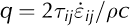is the internal heating due to the deformation. The vertical velocity w can be obtained from the horizontal velocities (Eqn (2)) based on the assumption that ice is incompressible.

Two boundary conditions are required to solve Eqn (9). At the surface, the temperature is taken from the model input. At the base, the temperature is determined as

(10)

T_pmpis the pressure-melting point. G is the basal geothermal heat flux (Table 1).

The shear stress τ_ij is calculated in terms of ice density ρ, the acceleration due to gravity g, the depth h and the surface slope α_i:

(11)

In Eqn (5) the longitudinal strain rate is involved in the shear strain rate to take account of the variations of flow properties and stresses along ice flow. The longitudinal strain rate is the gradient of the horizontal velocity

(12)

It can be expressed as

(13)

which indicates that the flow law (Eqn (5)) also includes the effect of the shear stress and the longitudinal stress gradients which are considered to play an important role at some places in the ice sheet, such as the areas of rough bedrock, fast ice flow or ice divides (Reference BuddBudd, 1971;Reference PattynPattyn and others, 2008). If is not included in Eqn (5) the flow law simplifies to a shallow-ice approximation form (Reference HutterHutter, 1983):

(14)

In this study we used the anisotropic ice flow law (Eqn (5)) and Eqns (1-12) to solve the ice thickness, shear and longitudinal strain rates, enhancement factors, temperatures, velocities, shear and longitudinal stresses.

Perturbation Experiment

The perturbations are taken from the difference of the ice- thickness changes (dH_bd/dt) below 2000 m elevation between ICESat (2003-07) and ERS (1992-2002), which represent the thickness change since 2003 (Reference ZwallyZwally and others, 2011). dH_bd/dt includes the combined dynamic and ablation terms (dH_bd/dt ≡ dH_d/dt + dH_b/dt). In the ablation zone, dH_bd/dt includes contributions from both ice dynamics (dH_d/dt) and melt (dH_b/dt). In the accumulation zone, dHbd/dt contains only the dynamic term (Reference Li and ZwallyLi and Zwally, 2011). The decrease of dH_bd/dt above 2000 m is considered to be a result of the inland propagation from the mass loss at lower elevations of the ice sheet. At some locations (mainly in the north) the perturbations are small and positive, which would cause dynamic thickening. To emphasize the stronger dominant impacts of the mass losses, we only use the gridpoints with negative perturbations. All positive perturbations are set to zero (Fig. 1b).

The experiment is intended to answer two questions: (1) How far and how rapidly will the strong mass loss from the coastal regions propagate inland? (2) How many years will the impact remain?

We set up the modeling runs in three steps. The first step is to establish a steady-state ice sheet which corresponds to present-day conditions (Fig. 2), using the present-day basaltopography (Reference Bamber, Layberry and GogineniBamber and others, 2001), surface mass balance (updated from Reference Zwally and GiovinettoZwally and Giovinetto, 2000), surface temperature and balance velocity. Derived balance velocity is based on the ICESat observed thickness (http://nsidc.org/data/nsidc-0304.html) and present-day surface mass balance using the scheme from Reference Budd and WarnerBudd and Warner (1996). To establish the present-day steady-state ice sheet (Fig. 2b and d), the model iterates on the governing equations (Reference Wang and WarnerWang and Warner, 1999), with the balance velocity (Fig. 2c) as a target. To compensate for any overestimated velocity without tuning any parameter in the flow law, we adopted the scheme from Reference Wang and WarnerWang and Warner (1999) by discounting integration of shear strain rate near the base of the ice sheet to match the balance velocity (Fig. 2c). This treatment produces strain-rate profiles with a band of high shear above the bedrock which can be compared with observations (e.g. Reference Wang and WarnerWang and Warner, 1999, Fig. 3; Reference Wang, Zwally, Abdalati and LuoWang and others, 2002b, fig. 4).

Fig. 2.

Initial state of the Greenland ice sheet for perturbation experiment. (a) Thickness derived from ICESat observation (http://nsidc.org/data/nsidc-0304.html). (b) Modeled thickness. (c) Derived balance velocity based on the ICESat observed thickness and present-day surface mass balance. (d) Modeled depth-averaged horizontal velocity. The 2000 m contour and equilibrium line are shown as a dotted line and dashed line, respectively.

Fig. 3.

(a) The rate of ice-thickness change averaged in 400 m elevation bands over the ice sheet versus elevations from the observations and the modeled results after 10year perturbation (Fig. 1c) over the whole ice sheet (GIS, black solid line) and drainage system 3 (DS3, red dashed line) which shows the stronger propagation. (b) Corresponding depth-averaged horizontal velocities. The ranges of perturbation (<2000 m elevation) and propagation (>2000 m elevation) are shown by the arrows.

Fig. 4.

Modeled ice-thickness changes with time (log scale) at four selected locations along the flowline in West Greenland (see Fig. 1c): (a) at the perturbation region; (b-d) at ~100km (b), ~200km (c) and ~400km (d) upstream from the perturbation region. The insets in (c) and (d) plot the time using a linear scale to show the time when the maximum thinning rates are reached.

In the second step, we put in the perturbations (Fig. 1b) and run the model for 10 years. The modeled results are compared with the observations (dH_bd/dt). The third step is set up to answer the question of how many years the impact is sustained after the perturbations are switched off by running the model forward 100 ka. The surface mass balance and temperature remain unchanged, which allows us to examine the impact from an isolated 10 year perturbation of the thickness. The model does not include an ice-front calving process. dH_bd/dt is small and the total thinning for a 10year perturbation at any perturbation gridpoint is a small portion of the thickness. Therefore, we treat the marginal ice edge as steady-state during the experimental period.

The model has a horizontal resolution of 50 km, compatible with the resolution of the observations, and 31 evenly spaced vertical layers. The time-steps are 1 year. The physical parameters used in the model are listed in Table 1. A finite-difference technique is used to solve the equations.

Results and Discussion

The modeled results after 10 years of perturbation input show that the observed strong mass loss at low elevations certainly causes interior ice-sheet thinning (Figs 1c and 3a). The dynamic propagation penetrates deep into the ice sheet, to almost the highest elevations. The modeled thinning pattern (Fig. 1c) over the ice sheet is in agreement with the observations (Fig. 1a), showing that enhanced thinning mainly occurs in the west and east, as well as in the southeast. In contrast, the thinning is least in the north and southwest. This implies that satellite-observed thinning (or reduced thickening) in the higher elevations of the ice sheet is likely induced by the extensive mass loss at the margins during the past decade or so.

The stronger propagation (Fig. 3a) corresponding to the higher horizontal velocities (Fig. 3b) in drainage system 3 indicates that faster ice flow enhances the propagation. The lack of resolution of basal troughs at 50 km grid spacing may result in reducing the speed of the propagation, as the deep troughs lead to higher driving stresses and warmer ice and therefore faster ice flow and stronger propagation. Improvement of the modeling spatial and temporal resolutions may enhance the propagation and reduce the discrepancies in the thinning rates between the modeled results and the observations (Fig. 3a).

After the perturbations are switched off, the ice sheet in the perturbation region starts to grow at a very high rate and then slowly returns to the previous steady state (Fig. 4a), while the ice sheet in the propagation region keeps thinning before recovering (Fig. 4 b-d). The maximum thinning rates occur after 1, 55 and 350 years (i.e. years 11, 65 and 360 in Fig. 4 b-d) at 100, 200 and 400 km upstream, respectively, showing a propagation wave: the farther from the perturbation region, the later the response occurs. The thickening rates during the recovery period are low compared with the ice loss rates during the period of thinning, so the ice sheet takes longer to return to its pre-perturbation state than it did to reach the thinnest state.

The changes in ice-sheet mass through time (Fig. 5) show the impact of the 10year perturbations. In the first 10years, the interior of the ice sheet (propagation region shown as red line) starts thinning slowly through the dynamic propagation along with a rapid mass loss over the whole ice sheet (black line) mainly due to the applied perturbations. While the whole ice sheet starts to grow back from the 11th year, when the perturbations are switched off at a total mass loss of 1300Gt, the interior ice sheet keeps thinning until ~300 years due to dynamic propagation. After reaching the maximum mass loss of 200Gt, the interior ice sheet also starts thickening. Both the interior and low-elevation regions reach the steady state again at ~10ka. Figure 5 illustrates that the strongest impact of the 10 year perturbations on the interior ice sheet occurs at ~300years and the impact is sustained for 10ka until full ice-sheet dynamic recovery. This result indicates that even if the large mass losses at the margins of the GIS ended today, the interior ice sheet would keep thinning for another 300years and the ice sheet would take thousands of years to recover fully.

Fig. 5.

Modeled ice-sheet mass change over the whole ice sheet (black line) and the ice sheet above 2000 m elevation (red line) as a function of time (a) in log scale for 10 ka and (b) in linear scale for the first 400 years, showing the times when the maximum mass losses are reached. The left-hand labels indicate the mass change relative to the maximum mass loss. The right-hand labels indicate the total mass loss (Gt) from the steady state for the whole ice sheet (black numbers) and for the ice sheet above 2000 m elevation (red numbers).

Conclusions

We used observed thinning rates below 2000 m elevation as the input to perturb the model to assess the inland propagation of the dynamic changes in the GIS. The model runs started from an initial present-day steady-state ice sheet with the perturbation applied for 10 years and then continued to 100 ka after the perturbations were switched off. The results show that the dynamic propagation penetrates deep into the interior ice sheet and that thinning is obvious within 10 years of the perturbation. The modeled thinning pattern over the ice sheet is in agreement with the observations: enhanced inland thinning mainly occurs in the western and eastern and, to some extent, the southeastern regions of the ice sheet. This implies that the strong mass loss since the early 2000s at the margins has had a dynamic impact on the entire GIS. The strongest impact for an isolated 10 year perturbation occurs at 300 years and it takes 10 ka for complete dynamic recovery. We conclude that the interior ice response to the changes at the ice-sheet margins is more rapid than generally expected and the dynamic impact will be sustained for a long period.