


1 Introduction
We investigate a mathematical model of interactions between colloid particles immersed in a nematic liquid crystal. Nematic liquid crystals are characterized by their orientational order: one can think of elongated molecules which tend to align along a common direction. Each immersed particle distorts this alignment at long range, inducing interactions with the other particles. When the sizes of the particles are much smaller than the distances between them, the physics literature develops an electrostatic analogy to describe their interactions, see [Reference Brochard and de Gennes5, Reference Ramaswamy, Nityananda, Raghunathan and Prost13, Reference Lubensky, Pettey, Currier and Stark10] and the survey [Reference Muševič12, § 2]. That analogy relies on linearizing, away from the particles, the equations which describe nematic alignment at equilibrium. Our main result gives an estimate of the error introduced by this linearization, under precise modeling assumptions which we describe next. From a purely mathematical viewpoint, this physical model corresponds to $\mathbb S^2$
-valued harmonic maps and our study explores a new perspective on those classical geometric objects, namely the dependence of their energy on the shape of the domain.
$\mathbb S^2$
-valued harmonic maps and our study explores a new perspective on those classical geometric objects, namely the dependence of their energy on the shape of the domain.
We use the simplest order parameter to describe the nematic phase: a unit vector $n\in \mathbb S^2$
indicating the direction of alignment. A liquid crystal filling a domain
$n\in \mathbb S^2$
indicating the direction of alignment. A liquid crystal filling a domain $\Omega \subset {\mathbb R}^3$
is described by a map
$\Omega \subset {\mathbb R}^3$
is described by a map $ n\colon \Omega \to \mathbb S^2$
, and we assume that its energy is given by
$ n\colon \Omega \to \mathbb S^2$
, and we assume that its energy is given by
 $$ \begin{align*} E(n)=\int_{\Omega}|\nabla n|^2\, dx +F(n_{\lfloor \partial\Omega})\,, \end{align*} $$
for some $F\colon H^{1/2}(\partial \Omega ;\mathbb S^2)\to [0,+\infty ]$
which accounts for the anchoring of liquid crystal molecules at the domain boundary. Note that minimizing configurations satisfy the harmonic map equation
$F\colon H^{1/2}(\partial \Omega ;\mathbb S^2)\to [0,+\infty ]$
which accounts for the anchoring of liquid crystal molecules at the domain boundary. Note that minimizing configurations satisfy the harmonic map equation $-\Delta n=|\nabla n|^2n$
in
$-\Delta n=|\nabla n|^2n$
in $\Omega $
.
$\Omega $
.
Here we consider domains $\Omega $
and anchoring energies F of a specific form, to model a system with N foreign particles, all of the same small size
$\Omega $
and anchoring energies F of a specific form, to model a system with N foreign particles, all of the same small size $\rho>0$
, but not necessarily the same shape, see Figure 1. To be precise, the liquid crystal occupies the exterior domain
$\rho>0$
, but not necessarily the same shape, see Figure 1. To be precise, the liquid crystal occupies the exterior domain
 $$ \begin{align*} \Omega_\rho ={\mathbb R}^3\setminus \bigcup_{j=1}^N \omega_{j,\rho}, \qquad \omega_{j,\rho} =x_j +\rho\,\hat \omega_j\,, \end{align*} $$
for fixed particle centers $x_1,\ldots ,x_N\in {\mathbb R}^3$
and smooth open sets
$x_1,\ldots ,x_N\in {\mathbb R}^3$
and smooth open sets
 $$ \begin{align*} \hat \omega_j\subset B_1 \subset{\mathbb R}^3\,, \qquad \text{for } j=1,\ldots,N\,. \end{align*} $$
These open sets represent the particles after zooming in at scale $\rho $
.
$\rho $
.
General setup for Theorem 1.1.

Rescaling by half the fixed minimal distance between these centers, we assume without loss of generality that they satisfy
 $$ \begin{align*} |x_i-x_j|\geq 2\qquad\forall i\neq j \in\lbrace 1,\ldots,N\rbrace\,. \end{align*} $$
We endow each rescaled particle $\hat \omega _j$
with an anchoring energy
$\hat \omega _j$
with an anchoring energy
 $$ \begin{align*} & \widehat F_j\colon H^{1/2}(\partial\hat\omega_j;\mathbb S^2)\to [0,\infty], \quad\text{ weakly lower semicontinuous}, \end{align*} $$
with nonempty domain $\lbrace \widehat F_j<\infty \rbrace \subset H^{1/2}(\partial \hat \omega _j;\mathbb S^2)$
, and assume that anchoring at the boundary of each small particle
$\lbrace \widehat F_j<\infty \rbrace \subset H^{1/2}(\partial \hat \omega _j;\mathbb S^2)$
, and assume that anchoring at the boundary of each small particle $\omega _{j,\rho }$
is described by the rescaled energy
$\omega _{j,\rho }$
is described by the rescaled energy
 $$ \begin{align*} F_{j,\rho}(n_{\lfloor\partial\omega_{j,\rho}})=\widehat F_j(\hat n^\rho_{j\lfloor\partial\hat\omega_j}),\qquad \hat n_j^\rho(\hat x) =n(x_j +\rho \, \hat x) \,. \end{align*} $$
Examples of admissible anchoring energies $\widehat F_j$
are given in [Reference Alama, Bronsard, Lamy and Venkatraman2, § 1.2]. They include familiar examples of strong anchoring (Dirichlet conditions) and weak anchoring (enforced by a surface energy). With these notations, the energy of a map
$\widehat F_j$
are given in [Reference Alama, Bronsard, Lamy and Venkatraman2, § 1.2]. They include familiar examples of strong anchoring (Dirichlet conditions) and weak anchoring (enforced by a surface energy). With these notations, the energy of a map $n\colon \Omega _\rho \to \mathbb S^2$
is given by
$n\colon \Omega _\rho \to \mathbb S^2$
is given by
 $$ \begin{align} E_\rho(n)=\frac{1}{\rho}\int_{\Omega_\rho}|\nabla n|^2\, dx +\sum_{j=1}^N F_{j,\rho}(n_{\lfloor\partial\omega_{j,\rho}})\,. \end{align} $$
We impose far-field alignment along a fixed orientation $n_\infty \in \mathbb S^2$
via the condition
$n_\infty \in \mathbb S^2$
via the condition
 $$ \begin{align} \int_{\Omega_\rho}\frac{|n(x)-n_\infty|^2}{1+|x|^2}\, dx <\infty\,. \end{align} $$
Existence of a minimizer of $E_\rho $
under this far-field alignment constraint can be proved exactly as in [Reference Alama, Bronsard, Lamy and Venkatraman2, § 1.2] for a single particle. Our main result is an asymptotic expansion, as
$E_\rho $
under this far-field alignment constraint can be proved exactly as in [Reference Alama, Bronsard, Lamy and Venkatraman2, § 1.2] for a single particle. Our main result is an asymptotic expansion, as $\rho \to 0$
, of the minimal energy
$\rho \to 0$
, of the minimal energy $E_\rho $
. That expansion depends on minimizers of the single-particle problems
$E_\rho $
. That expansion depends on minimizers of the single-particle problems
 $$ \begin{align} & \mu_j = \min \bigg\lbrace \widehat E_j(n) \colon \int_{{\mathbb R}^3\setminus\hat\omega_j} \!\! \frac{|n-n_\infty|^2}{1+|x|^2}\, dx <\infty \bigg\rbrace\,, \\ &\text{where } \widehat E_j(n) = \int_{{\mathbb R}^3\setminus \hat\omega_j}|\nabla n|^2\, dx +\widehat F_j(n_{\lfloor\partial\hat\omega_j}) \,. \nonumber \end{align} $$
It is shown in [Reference Alama, Bronsard, Lamy and Venkatraman2] that any minimizer $\hat m_j$
of (1.3) has a far-field expansion
$\hat m_j$
of (1.3) has a far-field expansion
 $$ \begin{align} \hat m_j(x) =n_\infty +\frac{v_j}{|x|} +\mathcal O\Big(\frac{1}{|x|^2}\Big)\qquad \text{as }|x|\to +\infty\,, \end{align} $$
for some $v_j\in {\mathbb R}^3$
orthogonal to
$v_j\in {\mathbb R}^3$
orthogonal to $n_\infty $
. The vector
$n_\infty $
. The vector $v_j$
can be interpreted as a torque applied by the particle
$v_j$
can be interpreted as a torque applied by the particle $\hat \omega _j$
on the nematic background [Reference Brochard and de Gennes5], see also [Reference Alama, Bronsard, Lamy and Venkatraman2, Theorem 2]. The effective interaction between two particles depends on these vectors
$\hat \omega _j$
on the nematic background [Reference Brochard and de Gennes5], see also [Reference Alama, Bronsard, Lamy and Venkatraman2, Theorem 2]. The effective interaction between two particles depends on these vectors $v_j$
.
$v_j$
.
Theorem 1.1. There exist minimizers $\hat m_j$
of the single-particle problems (1.3) such that the minimum of
$\hat m_j$
of the single-particle problems (1.3) such that the minimum of $E_\rho $
over maps
$E_\rho $
over maps $n\colon \Omega _\rho \to \mathbb {S}^{ 2}$
with far-field alignment (1.2) satisfies
$n\colon \Omega _\rho \to \mathbb {S}^{ 2}$
with far-field alignment (1.2) satisfies
 $$ \begin{align} \min E_\rho & =\sum_{j=1}^N \mu_j -4\pi\rho\sum_{i\neq j} \frac{\langle v_i,v_j\rangle}{|x_i-x_j|} + o(\rho)\qquad\text{as }\rho\to 0\,, \end{align} $$
where $\mu _j=\widehat E_j(\hat m_j)$
is the minimal single-particle energy (1.3), and
$\mu _j=\widehat E_j(\hat m_j)$
is the minimal single-particle energy (1.3), and $v_j\in n_\infty ^\perp $
is defined by the asymptotic expansion (1.4) of
$v_j\in n_\infty ^\perp $
is defined by the asymptotic expansion (1.4) of $\hat m_j$
.
$\hat m_j$
.
The interaction potential given by the term of order $\rho $
in the asymptotic expansion of Theorem 1.1 corresponds to solving the Poisson equation with singular source term
$\rho $
in the asymptotic expansion of Theorem 1.1 corresponds to solving the Poisson equation with singular source term
 $$ \begin{align} \Delta u_\rho = \sum_{j=1}^N 4\pi \rho v_j\delta_{x_j}\quad\text{ in }{\mathbb R}^3\,, \quad \text{that is,} \quad u_\rho(x) =\rho\sum_{j=1}^N \frac{v_j}{|x-x_j|}\,. \end{align} $$
The infinite energy of $u_\rho $
can indeed be renormalized to give
$u_\rho $
can indeed be renormalized to give
 $$ \begin{align*} \lim_{\sigma\to 0} \bigg( \frac{1}{\rho}\int_{{\mathbb R}^3\setminus \bigcup B_\sigma(x_j)}\!|\nabla u_\rho|^2\, dx -\frac{4\pi}{\sigma}\rho\sum_{j=1}^N |v_j|^2\bigg) =-4\pi\rho\sum_{i\neq j}\frac{\langle v_i,v_j\rangle}{|x_i-x_j|} \,. \end{align*} $$
This can be interpreted as follows:
-
• away from the particles, the harmonic map equation $-\Delta n=|\nabla n|^2 n$
is linearized around the uniform state
$n_\infty $
, which corresponds to writing
$n\approx n_\infty +u$
and
$-\Delta u\approx 0$
;
$-\Delta n=|\nabla n|^2 n$
is linearized around the uniform state
$n_\infty $
, which corresponds to writing
$n\approx n_\infty +u$
and
$-\Delta u\approx 0$
; -
• the effect of the particle
$\omega _{j,\rho }$
is replaced by a singular source term at
$x_j$
, and that source term is chosen to match the far-field expansion (1.4) generated by the single particle.


This linearized description is the electrostatic analogy introduced in [Reference Brochard and de Gennes5] and further developed in [Reference Ramaswamy, Nityananda, Raghunathan and Prost13, Reference Lubensky, Pettey, Currier and Stark10]. The difference in energy between the (renormalized) linearized description and the original nonlinear problem is what we estimate in Theorem 1.1. This gives the asymptotic expansion (1.5), where all the nonlinearity of the original problem is concentrated in the presence of $\mu _j$
and
$\mu _j$
and $v_j$
, determined by the single-particle problem (1.3).
$v_j$
, determined by the single-particle problem (1.3).
A few comments about the vectors $v_j$
are in order. There is no guarantee that the problem (1.3) should have a unique minimizer, nor that different minimizers should have the same asymptotic expansion (1.4), so
$v_j$
are in order. There is no guarantee that the problem (1.3) should have a unique minimizer, nor that different minimizers should have the same asymptotic expansion (1.4), so $v_j$
may in principle not be uniquely determined by
$v_j$
may in principle not be uniquely determined by $\hat \omega _j$
,
$\hat \omega _j$
, $\widehat F_j$
, and
$\widehat F_j$
, and $n_\infty $
. The family of vectors
$n_\infty $
. The family of vectors $v_j$
appearing in Theorem 1.1 corresponds to any choice that minimizes the expression in the right-hand side of (1.5), see §4. Note however that we are not aware of any example of nonuniqueness. Moreover, the interpretation of
$v_j$
appearing in Theorem 1.1 corresponds to any choice that minimizes the expression in the right-hand side of (1.5), see §4. Note however that we are not aware of any example of nonuniqueness. Moreover, the interpretation of $v_j$
as a torque ensures its generic uniqueness, in the sense that, for fixed
$v_j$
as a torque ensures its generic uniqueness, in the sense that, for fixed $\hat \omega _j$
and
$\hat \omega _j$
and $\widehat F_j$
, almost every choice of
$\widehat F_j$
, almost every choice of $n_\infty \in \mathbb S^2$
determines a unique
$n_\infty \in \mathbb S^2$
determines a unique $v_j$
, see [Reference Alama, Bronsard, Lamy and Venkatraman2, Theorem 1.4]. In general we are not able to obtain an explicit expression of the vector
$v_j$
, see [Reference Alama, Bronsard, Lamy and Venkatraman2, Theorem 1.4]. In general we are not able to obtain an explicit expression of the vector $v_j$
, except in some simple cases where it is zero. One such case is when the boundary conditions are free; namely, if
$v_j$
, except in some simple cases where it is zero. One such case is when the boundary conditions are free; namely, if $\widehat F_j=0$
then any minimizer of (1.3) is constant equal to
$\widehat F_j=0$
then any minimizer of (1.3) is constant equal to $n_\infty $
and
$n_\infty $
and $v_j=0$
. A less trivial case is that of spherical particles: if both
$v_j=0$
. A less trivial case is that of spherical particles: if both $\hat \omega _j$
and
$\hat \omega _j$
and $\widehat F_j$
are invariant under all rotations, then
$\widehat F_j$
are invariant under all rotations, then $v_j=0$
, see [Reference Alama, Bronsard, Lamy and Venkatraman2, Corollary 1.8].
$v_j=0$
, see [Reference Alama, Bronsard, Lamy and Venkatraman2, Corollary 1.8].
Ideas of proof
The proof of Theorem 1.1 consists of two parts: an upper bound, which we prove by constructing a competitor, and a lower bound which we obtain via a precise description of minimizers $n_\rho $
.
$n_\rho $
.
The competitor we choose for the upper bound is equal to the single-particle minimizer $\hat m_j$
, suitably rescaled, in small regions
$\hat m_j$
, suitably rescaled, in small regions $B_\sigma (x_j)$
. Outside these balls, we take its
$B_\sigma (x_j)$
. Outside these balls, we take its ${\mathbb R}^3$
-valued harmonic extension (tending to
${\mathbb R}^3$
-valued harmonic extension (tending to $n_\infty $
at far field) and project it back onto
$n_\infty $
at far field) and project it back onto $\mathbb S^2$
. For a well-chosen
$\mathbb S^2$
. For a well-chosen $\sigma $
satisfying
$\sigma $
satisfying $\rho \ll \sigma \ll 1$
, the energy of the competitor is controlled by the right-hand side of our expansion (1.5).
$\rho \ll \sigma \ll 1$
, the energy of the competitor is controlled by the right-hand side of our expansion (1.5).
The lower bound is more challenging. Thanks to classical compactness properties of energy-minimizing maps, the blow-up at scale $\rho $
of a minimizer
$\rho $
of a minimizer $n_\rho $
around each particle, given by
$n_\rho $
around each particle, given by $\hat n_j^\rho (\hat x)=n_\rho (x_j +\rho \,\hat x)$
, converges in
$\hat n_j^\rho (\hat x)=n_\rho (x_j +\rho \,\hat x)$
, converges in $H^1_{\mathrm {loc}}$
to a single-particle minimizer
$H^1_{\mathrm {loc}}$
to a single-particle minimizer $\hat m_j(\hat x)$
. This provides the first term in the asymptotic expansion (1.5) and suggests a natural route to obtain the next term: show that
$\hat m_j(\hat x)$
. This provides the first term in the asymptotic expansion (1.5) and suggests a natural route to obtain the next term: show that $\hat n_j^\rho - \hat m_j$
is small enough in
$\hat n_j^\rho - \hat m_j$
is small enough in $B_{\sigma /\rho }$
to produce a negligible energy error, for an adequate scale
$B_{\sigma /\rho }$
to produce a negligible energy error, for an adequate scale $\sigma $
. If this were true, the conclusion would follow by using the energy of the harmonic extension of
$\sigma $
. If this were true, the conclusion would follow by using the energy of the harmonic extension of $n_\rho $
as a lower bound outside the regions
$n_\rho $
as a lower bound outside the regions $B_\sigma (x_j)$
. In other words, that natural route would require a quantitative rate for the convergence
$B_\sigma (x_j)$
. In other words, that natural route would require a quantitative rate for the convergence $\hat n_j^\rho \to \hat m_j$
. However, this convergence was obtained by weak compactness arguments, and quantifying it seems out of reach. Instead, we modify our approach in order to conclude without quantitative rates. This relies on the following two ingredients.
$\hat n_j^\rho \to \hat m_j$
. However, this convergence was obtained by weak compactness arguments, and quantifying it seems out of reach. Instead, we modify our approach in order to conclude without quantitative rates. This relies on the following two ingredients.
-
• The first is a compensation effect between the inner and outer regions: if
$\hat n_j^\rho $
is too different from
$\hat m_j$
near
$\partial B_{\sigma /\rho }$
, the energy of the harmonic extension of
$ n_\rho $
outside the regions
$B_\sigma (x_j)$
is increased by an amount which partly compensates the energy error inside
$B_\sigma (x_j)$
. This implies an improved lower bound for the full energy. As a result, showing that the error is negligible boils down to the estimate
$|\hat n_\rho ^j(\hat x)-\hat m_j(\hat x)| \ll 1/|\hat x|$
in the annulus
$B_{2\sigma /\rho }\setminus B_{\sigma /\rho }$
, for a choice of scale
$\sigma \ll 1$
in an adequate range. In terms of scaling, such estimate is consistent with the nonquantitative
$L^2$
convergence
$\nabla \hat n_j^\rho \to \nabla \hat m_j$
. In comparison, separate lower bounds in the inner and outer regions, without taking advantage of this compensation effect, would have required
$|\hat n_\rho ^j(x)-\hat m_j(x)| \ll \sqrt \rho /|\hat x|$
to make the error negligible. -
• The second ingredient is a far-field expansion for
$\hat n_j^\rho $
in large annuli, similar to the expansion (1.4) of
$\hat m_j$
. That far-field expansion eventually implies the estimate
$|\hat n_\rho ^j(x)-\hat m_j(x)| \ll 1/|\hat x|$
, hence the conclusion thanks to the first ingredient. The proof of the expansion (1.4) in [Reference Alama, Bronsard, Lamy and Venkatraman2] uses the fact that a classical harmonic function with finite energy in the exterior domain
${\mathbb R}^3\setminus B_\lambda $
only has radially decaying modes. Here, in order to adapt it to
$\hat n_j^\rho $
, the main difference is that we must take into account radially increasing modes which can occur in an annulus, and estimate them appropriately.


Related works
Estimating the minimal energy of harmonic maps in exterior domains, and interpreting it as an interaction energy, is a very natural mathematical problem. To the best of our knowledge, the perspective from which it has been addressed so far is different from the present one. We wish to recall here the seminal works [Reference Brezis, Coron and Lieb4] by Brezis, Coron, and Lieb in three dimensions, and [Reference Bethuel, Brezis and Hélein3, Chapter I] by Bethuel, Brezis, and Hélein in two dimensions. There, the objects of study are smooth $\mathbb S^2$
or
$\mathbb S^2$
or $\mathbb S^1$
-valued maps outside holes, and the authors investigate the minimal energy within a fixed homotopy class. At first sight, their holes play a role very similar to our particles. But here, on the contrary, our maps are not assumed to be smooth: near the particles they may have several singularities, about which our analysis says nothing quantitative. As a consequence, minimizing over a homotopy class would not even make sense in our setting, and instead, admissible competitors are constrained by the anchoring conditions. Finally, the results and methods in [Reference Brezis, Coron and Lieb4] and [Reference Bethuel, Brezis and Hélein3] are very different from each other but remain fundamentally nonlinear, while a linearization procedure is at the heart of the present work.
$\mathbb S^1$
-valued maps outside holes, and the authors investigate the minimal energy within a fixed homotopy class. At first sight, their holes play a role very similar to our particles. But here, on the contrary, our maps are not assumed to be smooth: near the particles they may have several singularities, about which our analysis says nothing quantitative. As a consequence, minimizing over a homotopy class would not even make sense in our setting, and instead, admissible competitors are constrained by the anchoring conditions. Finally, the results and methods in [Reference Brezis, Coron and Lieb4] and [Reference Bethuel, Brezis and Hélein3] are very different from each other but remain fundamentally nonlinear, while a linearization procedure is at the heart of the present work.
Note that in [Reference Bethuel, Brezis and Hélein3], the interaction energy is also obtained as the second term in an asymptotic expansion and is also of Coulomb type, but this comes from the fact that $\mathbb S^1$
-valued harmonic maps can be “lifted” to
$\mathbb S^1$
-valued harmonic maps can be “lifted” to ${\mathbb R}$
-valued harmonic maps, rather than a linearization around a uniform state as in the present work. The analysis in [Reference Bethuel, Brezis and Hélein3] has initiated a rich line of research, including generalizations to maps with values into general manifolds and maps defined on higher-dimensional domains or manifolds, and we do not attempt here to give a list of these generalizations.
${\mathbb R}$
-valued harmonic maps, rather than a linearization around a uniform state as in the present work. The analysis in [Reference Bethuel, Brezis and Hélein3] has initiated a rich line of research, including generalizations to maps with values into general manifolds and maps defined on higher-dimensional domains or manifolds, and we do not attempt here to give a list of these generalizations.
Finally, we mention the more recent papers [Reference Chandler and Spagnolie6, Reference Golovaty, Taylor, Venkatraman and Zarnescu8]. The paper [Reference Chandler and Spagnolie6] uses methods from complex analysis and analogies with potential flows in fluid dynamics to study a version of our problem in the plane. The paper [Reference Golovaty, Taylor, Venkatraman and Zarnescu8] considers interaction energies between particles in the so-called “paranematic” regime, in which nematic order is only felt at the boundaries of the particles. Consequently, the interaction energy is much more localized to essentially overlapping boundary layers, and the analysis is largely linear.
Further directions
The physics of nematic suspensions raises many mathematical questions, and we mention here a few that are directly linked with the present work.
We considered here the simplest model for the nematic phase. Replacing the isotropic Dirichlet energy by a general anisotropic energy with three elastic constants [Reference De Gennes and Prost7, § 3.1.2] would likely be achievable at the cost of a few technical adjustments. Adapting the present analysis to a Q-tensor model (necessary to describe more symmetric single-particle minimizers, see, e.g., [Reference Alama, Bronsard and Lamy1]), would require new ingredients to deal with the extra length scale of phase transitions which is present in that model.
Recall that the vectors $v_j$
in (1.5) can be interpreted as torques. As detailed in [Reference Alama, Bronsard, Lamy and Venkatraman2], it follows from that interpretation that, if the particles
$v_j$
in (1.5) can be interpreted as torques. As detailed in [Reference Alama, Bronsard, Lamy and Venkatraman2], it follows from that interpretation that, if the particles $\hat \omega _j$
are spherical, or if they are in an equilibrium orientation with respect to
$\hat \omega _j$
are spherical, or if they are in an equilibrium orientation with respect to $n_\infty $
, then all the vectors
$n_\infty $
, then all the vectors $v_j$
are zero. In that case, our asymptotic expansion (1.5) does not capture any interaction term. These would be described by a next-order expansion, as predicted by the electrostatic analogy [Reference Lubensky, Pettey, Currier and Stark10]. An estimate of the error in that next order expansion would be very interesting.
$v_j$
are zero. In that case, our asymptotic expansion (1.5) does not capture any interaction term. These would be described by a next-order expansion, as predicted by the electrostatic analogy [Reference Lubensky, Pettey, Currier and Stark10]. An estimate of the error in that next order expansion would be very interesting.
From the physical point of view, it is also highly relevant to consider systems which are not at elastic equilibrium: either because of other physical effects (as already present in the original work of Brochard and de Gennes [Reference Brochard and de Gennes5] where the particles are magnetic), or simply to describe time evolution. The present work can serve as a first step towards these more complex models.
Finally, the limit $N\to \infty $
is of course very natural to study. In that perspective, one goal could be to estimate the error in the continuum approximation proposed in [Reference Brochard and de Gennes5, § II.3]. Another goal could be to establish a link between nematic suspensions and infinite point systems of Coulomb gas type, as has been done for Ginzburg-Landau vortices, see the survey [Reference Serfaty15] and references therein.
$N\to \infty $
is of course very natural to study. In that perspective, one goal could be to estimate the error in the continuum approximation proposed in [Reference Brochard and de Gennes5, § II.3]. Another goal could be to establish a link between nematic suspensions and infinite point systems of Coulomb gas type, as has been done for Ginzburg-Landau vortices, see the survey [Reference Serfaty15] and references therein.
Plan of the article
In § 2 we establish preliminary estimates on the energy of harmonic functions in exterior domains. In § 3 we present the upper bound construction. In § 4 we establish the lower bound, thus proving Theorem 1.1. In the Appendices A and B we present for completeness some results about existence of decaying solutions to Poisson’s equation, and estimates on the decay of harmonic functions in annuli.
Notations
We write $A\lesssim B$
to denote
$A\lesssim B$
to denote $A\leq C B$
for a generic constant
$A\leq C B$
for a generic constant $C>0$
, independent of
$C>0$
, independent of $\rho $
, but which can depend on the fixed parameters of our problem: N,
$\rho $
, but which can depend on the fixed parameters of our problem: N, $\hat \omega _j$
,
$\hat \omega _j$
, $\widehat F_j$
,
$\widehat F_j$
, $n_\infty $
. We write
$n_\infty $
. We write $E_\rho (n;U)$
and
$E_\rho (n;U)$
and $\widehat E_j(m;V)$
to denote restrictions of the integrals defining these energies to subsets U included in the interior of
$\widehat E_j(m;V)$
to denote restrictions of the integrals defining these energies to subsets U included in the interior of $\Omega _\rho $
or V included in the interior of
$\Omega _\rho $
or V included in the interior of ${\mathbb R}^3\setminus \hat \omega _j$
. We will also use the notation
${\mathbb R}^3\setminus \hat \omega _j$
. We will also use the notation $E_\rho (n;U)$
for subsets
$E_\rho (n;U)$
for subsets $U\subset \Omega _\rho $
which contain
$U\subset \Omega _\rho $
which contain $\partial \omega _{j,\rho }$
for some
$\partial \omega _{j,\rho }$
for some $j\in \lbrace 1,\ldots , N\rbrace $
, and in that case it is meant to incorporate the corresponding anchoring terms
$j\in \lbrace 1,\ldots , N\rbrace $
, and in that case it is meant to incorporate the corresponding anchoring terms $F_{j,\rho }(n_{|\partial \omega _{j,\rho }})$
. Similarly, for subsets
$F_{j,\rho }(n_{|\partial \omega _{j,\rho }})$
. Similarly, for subsets $V\subset {\mathbb R}^3\setminus \hat \omega _j$
which contain
$V\subset {\mathbb R}^3\setminus \hat \omega _j$
which contain $\partial \hat \omega _j$
, the notation
$\partial \hat \omega _j$
, the notation $\widehat E_j(m;V)$
is meant to incorporate the anchoring term
$\widehat E_j(m;V)$
is meant to incorporate the anchoring term $\widehat F_j(m_{|\partial \hat \omega _j})$
. We will often use the spherical variable
$\widehat F_j(m_{|\partial \hat \omega _j})$
. We will often use the spherical variable $\omega \in \mathbb S^2$
, not to be confused with the subsets
$\omega \in \mathbb S^2$
, not to be confused with the subsets $\omega _{j,\rho },\hat \omega _j\subset {\mathbb R}^3$
(which always come with a subscript, while
$\omega _{j,\rho },\hat \omega _j\subset {\mathbb R}^3$
(which always come with a subscript, while $\omega \in \mathbb S^2$
never does).
$\omega \in \mathbb S^2$
never does).
2 Prelude: harmonic extensions outside a union of small spheres
In this section we establish an estimate for the energy of harmonic functions u in the exterior domain
 $$ \begin{align*} U_\sigma={\mathbb R}^3\setminus \bigcup_{j=1}^N B_\sigma(x_j),\qquad\text{for some }\sigma\in (\rho,1/2)\,, \end{align*} $$
in terms of their boundary values on $\partial B_\sigma (x_j)$
that will be useful at several points in the proof of Theorem 1.1.
$\partial B_\sigma (x_j)$
that will be useful at several points in the proof of Theorem 1.1.
We first introduce some notations. We fix $\lbrace \Phi _k\rbrace _{k \in \mathbb {N}_0}$
an orthonormal Hilbert basis of
$\lbrace \Phi _k\rbrace _{k \in \mathbb {N}_0}$
an orthonormal Hilbert basis of $L^2(\mathbb S^2)$
which diagonalizes the Laplace-Beltrami operator,
$L^2(\mathbb S^2)$
which diagonalizes the Laplace-Beltrami operator,
 $$ \begin{align*} -\Delta_{\mathbb S^2}\Phi_k =\lambda_k \Phi_k,\qquad 0= \lambda_0 < \lambda_1\leq \lambda_2\leq \cdots \,. \end{align*} $$
The set $\lbrace \lambda _k\rbrace _{k\in \mathbb N_0}$
coincides with
$\lbrace \lambda _k\rbrace _{k\in \mathbb N_0}$
coincides with $\lbrace \ell ^2 + \ell \rbrace _{\ell \in \mathbb N_0}$
, and the eigenfunctions corresponding to
$\lbrace \ell ^2 + \ell \rbrace _{\ell \in \mathbb N_0}$
, and the eigenfunctions corresponding to $\ell ^2 + \ell $
span the homogeneous harmonic polynomials of degree
$\ell ^2 + \ell $
span the homogeneous harmonic polynomials of degree $\ell $
(which have dimension
$\ell $
(which have dimension $2\ell +1$
). The function
$2\ell +1$
). The function $\Phi _0$
is constant, equal to
$\Phi _0$
is constant, equal to $1/(2\sqrt \pi )$
. Solutions
$1/(2\sqrt \pi )$
. Solutions $f(r)$
of
$f(r)$
of $\Delta (f(r)\Phi _k(\omega ))=0$
in
$\Delta (f(r)\Phi _k(\omega ))=0$
in ${\mathbb R}^3\setminus \lbrace 0\rbrace $
are spanned by
${\mathbb R}^3\setminus \lbrace 0\rbrace $
are spanned by $f_\pm (r)=r^{\pm \gamma _k^\pm }$
, with
$f_\pm (r)=r^{\pm \gamma _k^\pm }$
, with
 $$ \begin{align*} \gamma_k^+ &= \sqrt{\frac 14 +\lambda_k} - \frac{1}{2} = \ell \quad \text{for }\lambda_k =\ell^2+\ell,\\ \gamma_k^- &= \sqrt{\frac 14 +\lambda_k} + \frac{1}{2} = \ell +1 \quad \text{for }\lambda_k =\ell^2+\ell. \end{align*} $$
These eigenfunctions satisfy the pointwise bound
 $$ \begin{align} |\nabla^\alpha\Phi_k| { \leq c_\alpha} \lambda_k^{\frac{1+\alpha}{2}} \qquad\forall \alpha\geq 0\,,\: \: k\geq 1\,, \end{align} $$
for some $c_\alpha>0$
. Indeed, for
$c_\alpha>0$
. Indeed, for $k\geq 1$
and any
$k\geq 1$
and any $\omega _0\in \mathbb S^2$
, in local coordinates around
$\omega _0\in \mathbb S^2$
, in local coordinates around $\omega _0$
we can consider the rescaled function
$\omega _0$
we can consider the rescaled function $\varphi (z) =\Phi _k(\omega _0 +z/\sqrt {\lambda _k})$
which satisfies
$\varphi (z) =\Phi _k(\omega _0 +z/\sqrt {\lambda _k})$
which satisfies $L \varphi =\varphi $
in a fixed ball
$L \varphi =\varphi $
in a fixed ball $B_1$
for some elliptic operator L (with smooth coefficients depending on the local coordinates). Elliptic estimates imply
$B_1$
for some elliptic operator L (with smooth coefficients depending on the local coordinates). Elliptic estimates imply $|\varphi (0)|^2\lesssim \int _{B_1}|\varphi |^2\, dz \lesssim \lambda _k\int _{\mathbb S^2}|\Phi _k|^2$
, hence
$|\varphi (0)|^2\lesssim \int _{B_1}|\varphi |^2\, dz \lesssim \lambda _k\int _{\mathbb S^2}|\Phi _k|^2$
, hence $|\Phi _k|\lesssim \lambda _k^{1/2}$
. This shows (2.1) for
$|\Phi _k|\lesssim \lambda _k^{1/2}$
. This shows (2.1) for $\alpha =0$
. The case of higher derivatives
$\alpha =0$
. The case of higher derivatives $\alpha \geq 1$
follows from elliptic estimates on
$\alpha \geq 1$
follows from elliptic estimates on $\mathbb S^2$
and the fact that
$\mathbb S^2$
and the fact that $(-\Delta _{\mathbb S^2})^{\beta }\Phi _k=\lambda _k^{\beta }\Phi _k$
for any integer
$(-\Delta _{\mathbb S^2})^{\beta }\Phi _k=\lambda _k^{\beta }\Phi _k$
for any integer $\beta \geq 1$
. (For instance, iterating the estimate
$\beta \geq 1$
. (For instance, iterating the estimate $\|\nabla ^2\varphi \|_{L^2}\leq c \|(-\Delta )\varphi \|_{L^2}$
implies
$\|\nabla ^2\varphi \|_{L^2}\leq c \|(-\Delta )\varphi \|_{L^2}$
implies $\|\nabla ^{2\beta }\varphi \|_{L^2}\leq c^\beta \|(-\Delta )^\beta \varphi \|_{L^2}$
for any smooth
$\|\nabla ^{2\beta }\varphi \|_{L^2}\leq c^\beta \|(-\Delta )^\beta \varphi \|_{L^2}$
for any smooth $\varphi $
on
$\varphi $
on $\mathbb S^2$
, hence
$\mathbb S^2$
, hence $\|\nabla ^{2\beta }\Phi _k\|_{L^2}\leq c^\beta \lambda _k^\beta $
. Then one may combine this with the Sobolev embedding
$\|\nabla ^{2\beta }\Phi _k\|_{L^2}\leq c^\beta \lambda _k^\beta $
. Then one may combine this with the Sobolev embedding $W^{4\alpha ,2}(\mathbb S^2)\subset W^{\alpha ,\infty }(\mathbb S^2)$
which provides the interpolation inequality
$W^{4\alpha ,2}(\mathbb S^2)\subset W^{\alpha ,\infty }(\mathbb S^2)$
which provides the interpolation inequality $\|\nabla ^\alpha \varphi \|_{L^\infty }\leq c_\alpha \|\varphi \|^{1-\theta }_{L^2} \|\nabla ^{4\alpha }\varphi \|^\theta _{L^2}$
for
$\|\nabla ^\alpha \varphi \|_{L^\infty }\leq c_\alpha \|\varphi \|^{1-\theta }_{L^2} \|\nabla ^{4\alpha }\varphi \|^\theta _{L^2}$
for $\theta =(1+\alpha )/4\alpha $
.)
$\theta =(1+\alpha )/4\alpha $
.)
Proposition 2.1. If $\Delta u=0$
in
$\Delta u=0$
in $U_\sigma ={\mathbb R}^3\setminus \bigcup _{j=1}^N B_\sigma (x_j)$
,
$U_\sigma ={\mathbb R}^3\setminus \bigcup _{j=1}^N B_\sigma (x_j)$
, $\int _{U_\sigma } |\nabla u|^2\, dx <\infty $
with
$\int _{U_\sigma } |\nabla u|^2\, dx <\infty $
with $|u|\to 0$
as
$|u|\to 0$
as $|x|\to \infty $
and
$|x|\to \infty $
and $u=g_j$
on
$u=g_j$
on $\partial B_\sigma (x_j)$
for
$\partial B_\sigma (x_j)$
for $j=1,\ldots ,N$
, with
$j=1,\ldots ,N$
, with
 $$ \begin{align*} g_j(x_j +\sigma\omega)=\sum_{k\geq 0}a_k^j \Phi_k(\omega), \end{align*} $$
then
 $$ \begin{align} \int_{U_\sigma}|\nabla u|^2\, dx & = \sigma\sum_j \sum_{k\geq 0} \gamma_k^-|a_k^j|^2 -\sigma^2\sum_j\sum_{i\neq j}\frac{ \langle a_0^i,a_0^j\rangle}{|x_i-x_j|} \nonumber \\ &\qquad +\mathcal O(\sigma^3) \|a\|^2_{\ell^2} \, , \end{align} $$
where $\|a\|^2_{\ell ^2} =\sum _{j} \|a^j\|^2_{\ell ^2} =\sum _j\sum _{k\geq 0} |a_k^j|^2$
is the squared
$\|a\|^2_{\ell ^2} =\sum _{j} \|a^j\|^2_{\ell ^2} =\sum _j\sum _{k\geq 0} |a_k^j|^2$
is the squared $\ell ^2$
norm of the (double index) sequence
$\ell ^2$
norm of the (double index) sequence $(a^j_k)_{j,k}$
.
$(a^j_k)_{j,k}$
.
Remark 2.2. One can also express all terms in the right-hand side of (2.2) directly in terms of the functions $g_j$
, since the spherical harmonic coefficients are equal to
$g_j$
, since the spherical harmonic coefficients are equal to
 $$ \begin{align*} a_k^j=\int_{\mathbb S^2} g_j(x_j +\sigma\omega)\,\Phi_k(\omega) \, d\mathcal H^2(\omega)\,, \end{align*} $$
and the squared $\ell ^2$
norm of
$\ell ^2$
norm of $(a^j_k)$
corresponds in particular to
$(a^j_k)$
corresponds in particular to
 $$ \begin{align*} \|a\|_{\ell^2}^2 =\frac{1}{\sigma^2}\sum_j \int_{\partial B_\sigma(x_j)} |g_j|^2\,d\mathcal H^2\,. \end{align*} $$
Proof of Proposition 2.1.
All objects considered in the proof depend on $\sigma $
but we do not make this dependence explicit in the notations for better readability – although we do keep careful track of it in the estimates. Consider
$\sigma $
but we do not make this dependence explicit in the notations for better readability – although we do keep careful track of it in the estimates. Consider $u_j$
the harmonic extension of
$u_j$
the harmonic extension of $g_j(x_j +\cdot )$
in
$g_j(x_j +\cdot )$
in ${\mathbb R}^3\setminus B_\sigma $
, given by
${\mathbb R}^3\setminus B_\sigma $
, given by
 $$ \begin{align} u_j(r\omega) =\sum_{k\geq 0} a_k^j \left(\frac\sigma r\right)^{\gamma_k^-}\Phi_k(\omega), \end{align} $$
and the function
 $$ \begin{align*} \tilde u(x)=\sum_{j=1}^N u_j(x-x_j)\,, \end{align*} $$
which is harmonic in $U_\sigma $
. The function
$U_\sigma $
. The function $\tilde u - u$
is harmonic in
$\tilde u - u$
is harmonic in $U_\sigma $
, and on
$U_\sigma $
, and on $\partial B_\sigma (x_j)$
it is equal to the restriction of a function
$\partial B_\sigma (x_j)$
it is equal to the restriction of a function $h_j$
smooth in
$h_j$
smooth in $B_1(x_j)$
and given by
$B_1(x_j)$
and given by
 $$ \begin{align} h_j(x_j+r\omega) & =\sum_{i\neq j} u_i(x_j-x_i +r \omega)\,, \end{align} $$
for all $r\in (0,1)$
. Since
$r\in (0,1)$
. Since $u_i$
is decaying, this boundary error is small for small
$u_i$
is decaying, this boundary error is small for small $\sigma $
, and therefore, its harmonic extension
$\sigma $
, and therefore, its harmonic extension $u-\tilde u$
is also small. Hence we expect that the energy of u should coincide, at leading order, with the energy of
$u-\tilde u$
is also small. Hence we expect that the energy of u should coincide, at leading order, with the energy of $\tilde u$
. We will see that this heuristic is correct, but we will also need to include next-order contributions to capture the second term in the right-hand side of (2.2). We start from the identity
$\tilde u$
. We will see that this heuristic is correct, but we will also need to include next-order contributions to capture the second term in the right-hand side of (2.2). We start from the identity
 $$ \begin{align} \int_{U_\sigma}|\nabla u|^2\, dx & = \int_{U_\sigma}|\nabla\tilde u|^2\, dx +\int_{U_\sigma} |\nabla\tilde u-\nabla u|^2\, dx \nonumber \\ &\quad +2\int_{U_\sigma} \langle \nabla u -\nabla\tilde u,\nabla \tilde u\rangle \, dx\,. \end{align} $$
The rest of the proof is structured as follows. In Step 0 we gather some estimates on the boundary error $h_j$
. In Step 1 we estimate the last integral in (2.5). The integral of
$h_j$
. In Step 1 we estimate the last integral in (2.5). The integral of $|\nabla \tilde u-\nabla u|^2$
is estimated in Step 2. In Step 3 we compute
$|\nabla \tilde u-\nabla u|^2$
is estimated in Step 2. In Step 3 we compute $\int |\nabla \tilde u|^2$
and finally conclude in Step 4.
$\int |\nabla \tilde u|^2$
and finally conclude in Step 4.
Step 0. Estimates of the boundary error.
Let $i\neq j$
, and
$i\neq j$
, and $\alpha \geq 0$
. Using that
$\alpha \geq 0$
. Using that $|x_i-x_j|\geq 2$
,
$|x_i-x_j|\geq 2$
, $|\nabla _\omega ^\alpha \Phi _k | {\leq c_\alpha } \lambda _k^{(1+\alpha )/2}$
and
$|\nabla _\omega ^\alpha \Phi _k | {\leq c_\alpha } \lambda _k^{(1+\alpha )/2}$
and $\gamma _k^-\lesssim 1+\sqrt {\lambda _k}$
we obtain, for all
$\gamma _k^-\lesssim 1+\sqrt {\lambda _k}$
we obtain, for all $x\in B_\sigma (x_j)$
,
$x\in B_\sigma (x_j)$
,
 $$ \begin{align*} |\nabla^\alpha u_i(x - x_i)| & \leq C_\alpha \sum_{k\geq 0}|a_k^i| \big(1+\lambda_k^{\frac{1+\alpha}{2}}\big) \sigma^{\gamma_k^-} \\ & \leq C_\alpha \sigma \|a^i\|_{\ell^2} \bigg(\sum_{k\geq 0} \big(1+\lambda_k^{1+\alpha}\big) \sigma^{2\gamma_k^--2}\bigg)^{1/2}\\ & \leq C_\alpha \sigma \|a^i\|_{\ell^2}\,. \end{align*} $$
The last inequality is valid because $\sigma \leq 1/2$
and
$\sigma \leq 1/2$
and $\gamma _k^-\geq 1$
. In particular we have
$\gamma _k^-\geq 1$
. In particular we have
 $$ \begin{align} \max_{0\leq\alpha\leq 4} \sup_{B_\sigma(x_j)} |\nabla^{\alpha} u_i(\cdot -x_i)| \lesssim \sigma \|a^j\|_{\ell^2}\,. \end{align} $$
Combining this bound with the definition (2.4) of the boundary error $h_j$
, we infer
$h_j$
, we infer
 $$ \begin{align} |h_j(x_j+\sigma\omega)-h_j(x_j)| & \lesssim \sigma \sum_{i\neq j} \sup_{B_\sigma(x_j)}|\nabla u_i(\cdot - x_i)| \lesssim \sigma^2 \|a\|_{\ell^2}\,, \end{align} $$
and
 $$ \begin{align} |\Delta_\omega^2 \left[h_j(x_j+\sigma\omega)-h_j(x_j)\right]| & \lesssim \sigma^4 \sum_{i\neq j} \max_{0\leq\alpha\leq 4} \sup_{B_\sigma(x_j)}|\nabla^4 u_i(\cdot - x_i)| \nonumber \\ & \lesssim \sigma^5 \|a\|_{\ell^2} \,. \end{align} $$
Step 1. Estimating $\int \langle \nabla u-\nabla \tilde u,\nabla \tilde u\rangle $
.
$\int \langle \nabla u-\nabla \tilde u,\nabla \tilde u\rangle $
.
Since $\tilde u$
is harmonic in
$\tilde u$
is harmonic in $U_\sigma $
and
$U_\sigma $
and $\tilde u -u=h_j$
on
$\tilde u -u=h_j$
on $\partial B_\sigma (x_j)$
, we have
$\partial B_\sigma (x_j)$
, we have
 $$ \begin{align*} & \int_{U_\sigma} \langle \nabla u -\nabla\tilde u,\nabla \tilde u\rangle \, dx =\int_{\partial U_\sigma} \langle u-\tilde u,\partial_\nu \tilde u\rangle \, d\mathcal H^2 \\ & =\sigma^2\sum_j\int_{\mathbb S^2}\langle h_j(x_j +\sigma\omega),(\omega\cdot\!\nabla) \tilde u(x_j+\sigma\omega)\rangle\, d\mathcal H^2(\omega) \\ & =\sigma^2\sum_j \int_{\mathbb S^2}\langle h_j(x_j +\sigma\omega),\partial_r u_j(\sigma\omega)\rangle\, d\mathcal H^2(\omega) \\ & \quad +\sigma^2\sum_j\sum_{\ell\neq j} \int_{\mathbb S^2} \langle h_j(x_j +\sigma\omega),(\omega\cdot\!\nabla) u_\ell(x_j-x_\ell+\sigma\omega)\rangle\, d\mathcal H^2(\omega). \end{align*} $$
To control the last integral we note that the estimate (2.6) from Step 0 implies
 $$ \begin{align*} & |h_j(x_j+\sigma\omega)| \lesssim \sigma N \|a\|_{\ell^2} \quad \text{and} \quad |\nabla u_\ell(x_j-x_\ell +\sigma\omega)| \lesssim \sigma \|a\|_{\ell^2}\,, \end{align*} $$
for all $j\neq \ell $
and
$j\neq \ell $
and $\omega \in \mathbb S^2$
. We deduce
$\omega \in \mathbb S^2$
. We deduce
 $$ \begin{align} & \int_{U_\sigma} \langle \nabla u -\nabla\tilde u,\nabla \tilde u\rangle \, dx \nonumber \\ & =\sigma^2\sum_j \int_{\mathbb S^2}\langle h_j(x_j+\sigma\omega),\partial_r u_j(\sigma\omega)\rangle\, d\mathcal H^2(\omega) +\mathcal O(\sigma^4) \|a\|^2_{\ell^2} \,. \end{align} $$
For all $j\in \lbrace 1,\ldots ,N\rbrace $
, using the explicit expression (2.3) of
$j\in \lbrace 1,\ldots ,N\rbrace $
, using the explicit expression (2.3) of $u_j(r\omega )$
we have
$u_j(r\omega )$
we have
 $$ \begin{align} & \int_{\mathbb S^2} \langle h_j(x_j+\sigma\omega),\partial_r u_j(\sigma\omega)\rangle\, d\mathcal H^2(\omega) \nonumber \\ & = -\frac{1}{\sigma}\sum_{k\geq 0} \gamma_k^- \int_{\mathbb S^2} \langle h_j(x_j+\sigma\omega),a_k^j \rangle \, \Phi_k(\omega)\, d\mathcal H^2(\omega) \nonumber \\ & = -\frac{1}{2\sqrt\pi\sigma} \int_{\mathbb S^2} \langle h_j(x_j),a_0^j \rangle \, d\mathcal H^2 \nonumber \\ & \quad -\frac{1}{\sigma}\sum_{k\geq 0} \gamma_k^- \big\langle a_k^j, \int_{\mathbb S^2} \big( h_j(x_j+\sigma\omega)-h_j(x_j)\big) \, \Phi_k(\omega)\, d\mathcal H^2(\omega) \big\rangle\,. \end{align} $$
For the last equality we used the fact that the spherical harmonics $\Phi _k$
of order
$\Phi _k$
of order $k\geq 1$
have zero average, while
$k\geq 1$
have zero average, while $\Phi _0$
is constant equal to
$\Phi _0$
is constant equal to $1/(2\sqrt \pi )$
. To control the last sum, we note that by the estimate (2.7) from Step 0 we have
$1/(2\sqrt \pi )$
. To control the last sum, we note that by the estimate (2.7) from Step 0 we have
 $$ \begin{align*} \Big| \int_{\mathbb S^2} \big( h_j(x_j+\sigma\omega)-h_j(x_j) \big) \, \Phi_0(\omega)\, d\mathcal H^2(\omega) \Big| & \lesssim \sigma^2 \|a\|_{\ell^2}\,, \end{align*} $$
and, for $k\geq 1$
, thanks to the fact that
$k\geq 1$
, thanks to the fact that $\Phi _k=\lambda _k^{-2}\Delta _\omega ^2\Phi _k$
and the estimate (2.8) from Step 0,
$\Phi _k=\lambda _k^{-2}\Delta _\omega ^2\Phi _k$
and the estimate (2.8) from Step 0,
 $$ \begin{align*} & \Big| \int_{\mathbb S^2} \big( h_j(x_j+\sigma\omega)-h_j(x_j) \big) \, \Phi_k(\omega)\, d\mathcal H^2(\omega) \Big| \\ & =\frac{1}{\lambda_k^2} \Big| \int_{\mathbb S^2} \big( h_j(x_j+\sigma\omega)-h_j(x_j)\big) \, \Delta^2_\omega\Phi_k(\omega)\, d\mathcal H^2(\omega) \Big| \\ & =\frac{1}{\lambda_k^2} \Big| \int_{\mathbb S^2} \Delta_\omega^2\big( h_j(x_j+\sigma\omega)-h_j(x_j)\big) \, \Phi_k(\omega)\, d\mathcal H^2(\omega) \Big| \lesssim \frac{\sigma^5 }{\lambda_k^2} \|a\|_{\ell^2}\,. \end{align*} $$
From this and the previous inequality for $k=0$
we infer
$k=0$
we infer
 $$ \begin{align*} & \bigg| \sum_{k\geq 0} \gamma_k^- \big\langle a_k^j, \int_{\mathbb S^2} \big( h_j(x_j+\sigma\omega)-h_j(x_j)\big) \, \Phi_k(\omega)\, d\mathcal H^2(\omega) \big\rangle \bigg| \\ &\qquad\qquad\qquad\lesssim \sigma^2 \|a\|_{\ell^2} |a_0^j| + \sigma^5 \|a\|_{\ell^2} \sum_{k\geq 1} \frac{\gamma_k^-}{\lambda_k^2}|a_k^j| \lesssim \sigma^2\|a\|_{\ell^2}^2\,. \end{align*} $$
The last inequality follows from the fact that $(\gamma _k^-/\lambda _k^2)^2\lesssim 1/\lambda _k^{3}$
is summable. Using this to estimate the last line of (2.10) we deduce
$(\gamma _k^-/\lambda _k^2)^2\lesssim 1/\lambda _k^{3}$
is summable. Using this to estimate the last line of (2.10) we deduce
 $$ \begin{align*} \int_{\mathbb S^2}\langle h_j(x_j+\sigma\omega),&\partial_r u_j(\sigma\omega)\rangle\, d\mathcal H^2(\omega) \\ & = -\frac{1}{2\sqrt\pi\sigma} \int_{\mathbb S^2} \langle h_j(x_j),a_0^j \rangle \, \, d\mathcal H^2(\omega) +\mathcal O(\sigma) \|a\|^2_{\ell^2} \\ & = -\frac{ 2\sqrt\pi}{\sigma} \sum_{i\neq j} u_i(x_j-x_i) +\mathcal O(\sigma) \|a\|^2_{\ell^2}\,. \end{align*} $$
The last equality follows from the expression (2.4) of $h_j$
and the fact that
$h_j$
and the fact that $|\mathbb S^2|=4\pi $
. Plugging this back into (2.9) gives
$|\mathbb S^2|=4\pi $
. Plugging this back into (2.9) gives
 $$ \begin{align} \int_{U_\sigma} \langle \nabla u -\nabla\tilde u,\nabla \tilde u\rangle \, dx & = -\sigma^2\sum_j \sum_{i\neq j} \frac {2\sqrt\pi}\sigma \langle u_i(x_j-x_i),a_0^j\rangle \nonumber \\ &\quad +\mathcal O(\sigma^3) \|a\|^2_{\ell^2} \,. \end{align} $$
Step 2. Estimating $\int |\nabla \tilde u - \nabla u|^2$
.
$\int |\nabla \tilde u - \nabla u|^2$
.
To bound the term $\int |\nabla \tilde u - \nabla u|^2$
, we recall that
$\int |\nabla \tilde u - \nabla u|^2$
, we recall that $\tilde u-u$
is harmonic, apply Lemma 2.3 below and use (2.6) to obtain
$\tilde u-u$
is harmonic, apply Lemma 2.3 below and use (2.6) to obtain
 $$ \begin{align} \int_{U_\sigma}|\nabla\tilde u -\nabla u|^2\, dx & \lesssim \sigma \sum_j \|h_j\|^2_{C^1(\partial B_\sigma(x_j))} \lesssim \sigma^3 \|a\|_{\ell^2}^2 \,. \end{align} $$
Step 3. Computing $\int |\nabla \tilde u|^2$
.
$\int |\nabla \tilde u|^2$
.
Since $\tilde u$
is harmonic, we have
$\tilde u$
is harmonic, we have
 $$ \begin{align*} \int_{U_\sigma}|\nabla\tilde u|^2\, dx & =\int_{\partial U_\sigma} \langle \tilde u,\partial_\nu \tilde u\rangle \,d\mathcal H^2 = \sigma^2\sum_{j,\ell,\ell'} I_j[u_\ell,u_{\ell'}], \end{align*} $$
where, for $ j,\ell ,\ell '\in \lbrace 1,\ldots ,N\rbrace $
,
$ j,\ell ,\ell '\in \lbrace 1,\ldots ,N\rbrace $
,
 $$ \begin{align*} I_j[u_\ell,u_{\ell'}] &= \frac{1}{\sigma^2} \int_{\partial B_\sigma(x_j)} \langle u_\ell(\cdot -x_\ell),\partial_\nu [u_{\ell'}(\cdot -x_{\ell'})]\rangle \,d\mathcal H^2 \nonumber \\ & =- \int_{\mathbb S^2} \big\langle u_\ell(x_j-x_\ell +\sigma\omega), (\omega\cdot\!\nabla)u_{\ell'}(x_j-x_\ell' +\sigma\omega) \big\rangle \, d\mathcal H^2(\omega). \end{align*} $$
Since $u_\ell $
is small near
$u_\ell $
is small near $x_j-x_\ell $
for
$x_j-x_\ell $
for $j\neq \ell $
, the magnitude of this integral depends a lot on whether
$j\neq \ell $
, the magnitude of this integral depends a lot on whether $\ell ,\ell '$
are equal to j. The main order terms will correspond to
$\ell ,\ell '$
are equal to j. The main order terms will correspond to $\ell =\ell '=j$
, the next-order to
$\ell =\ell '=j$
, the next-order to $\ell \neq \ell '=j$
, and all other terms will be negligible for our purposes. We present next the estimates of each type of term.
$\ell \neq \ell '=j$
, and all other terms will be negligible for our purposes. We present next the estimates of each type of term.
For $\ell =\ell '=j$
, using the explicit expression (2.3) of
$\ell =\ell '=j$
, using the explicit expression (2.3) of $u_j(r\omega )$
we have
$u_j(r\omega )$
we have
 $$ \begin{align*} I_j[u_j,u_j] &= - \int_{\mathbb S^2}\langle u_j(\sigma\omega),\partial_r u_j(\sigma\omega)\rangle\, d\mathcal H^2(\omega) = \frac 1\sigma\sum_{k\geq 0}\gamma_k^- |a_k^j|^2 \,. \end{align*} $$
For $\ell \neq j$
and
$\ell \neq j$
and $\ell '=j$
, using again the explicit expression (2.3) of
$\ell '=j$
, using again the explicit expression (2.3) of $u_j(r\omega )$
, and the fact that
$u_j(r\omega )$
, and the fact that $\Phi _0=1/(2\sqrt \pi )$
while
$\Phi _0=1/(2\sqrt \pi )$
while $\Phi _k$
has zero average for
$\Phi _k$
has zero average for $k\geq 1$
, we find
$k\geq 1$
, we find
 $$ \begin{align*} &I_j[u_\ell,u_j] = -\int_{\mathbb S^2} \big\langle u_\ell(x_j-x_\ell +\sigma\omega),\partial_r u_j(\sigma\omega)\rangle\, d\mathcal H^2(\omega) \\ & =\frac 1\sigma \sum_{k\geq 0} \gamma_k^- \int_{\mathbb S^2} \big\langle u_\ell(x_j-x_\ell +\sigma\omega), a_k^j\rangle \, \Phi_k(\omega) \, d\mathcal H^2(\omega) \\ & =\frac{2\sqrt\pi}{\sigma}\langle u_\ell(x_j-x_\ell),a_0^j\rangle \\ & \quad +\frac 1\sigma \sum_{k\geq 1} \gamma_k^- \int_{\mathbb S^2} \big\langle u_\ell(x_j-x_\ell +\sigma\omega)-u_\ell(x_j-x_\ell), a_k^j\rangle \, \Phi_k(\omega) \, d\mathcal H^2(\omega)\,. \end{align*} $$
The last line can be estimated as in Step 1 for the last sum in (2.10), and we deduce
 $$ \begin{align*} I_j[u_\ell,u_j] & =\frac{2\sqrt\pi}{\sigma}\langle u_\ell(x_j-x_\ell),a_0^j\rangle +\mathcal O(\sigma)\|a\|^2_{\ell^2} \qquad\text{ for }\ell\neq j\,. \end{align*} $$
For $\ell =j$
and
$\ell =j$
and $\ell '\neq j$
we find, using the explicit expression (2.3) of
$\ell '\neq j$
we find, using the explicit expression (2.3) of $u_j(r\omega )$
, and the estimate (2.6) from Step 0,
$u_j(r\omega )$
, and the estimate (2.6) from Step 0,
 $$ \begin{align*} I_j[u_j,u_{\ell'}] & = \int_{\mathbb S^2} \big\langle u_j(\sigma\omega),(\omega\cdot\!\nabla) u_{\ell'}(x_j-x_{\ell'}+\sigma\omega)\big\rangle \, d\mathcal H^2(\omega) \\ & =\sum_{k\geq 0} \int_{\mathbb S^2} \big\langle a_k^j,(\omega\cdot\!\nabla) u_{\ell'}(x_j-x_{\ell'}+\sigma\omega)\big\rangle\,\Phi_k(\omega) \, d\mathcal H^2(\omega) \\ & =\mathcal O(\sigma)\|a\|^2_{\ell^2}\,. \end{align*} $$
Finally, for $\ell ,\ell '\neq j$
, we can directly use (2.6) to deduce
$\ell ,\ell '\neq j$
, we can directly use (2.6) to deduce
 $$ \begin{align*} I_j[u_\ell,u_\ell'] =\mathcal O(\sigma^2)\|a\|_{\ell^2}^2\,. \end{align*} $$
Gathering all these estimates on the integrals $I_j[u_\ell ,u_{\ell '}]$
, we obtain
$I_j[u_\ell ,u_{\ell '}]$
, we obtain
 $$ \begin{align} \int_{U_\sigma}|\nabla \tilde u|^2\, dx & =\sigma^2\sum_{j,\ell,\ell'}I_j[u_\ell,u_{\ell'}] \nonumber \\ & = \sigma\sum_j \sum_{k\geq 0}\gamma_k^- |a_k^j|^2 + \sigma^2 \sum_j \sum_{\ell\neq j}\frac{2\sqrt\pi}{\sigma} \langle u_\ell(x_j-x_\ell),a_0^j\rangle \nonumber \\ & \quad + \mathcal O(\sigma^3) \|a\|_{\ell^2}^2\,. \end{align} $$
Step 4. Conclusion.
Inserting Equations (2.11),(2.12) and (2.13) of Steps 1-3 into (2.5), we end up with
 $$ \begin{align*} \int_{U_\sigma}|\nabla\tilde u|^2\, dx & = \sigma\sum_j \sum_{k\geq 0} \gamma_k^-|a_k^j|^2 -\sigma^2\sum_j\sum_{\ell\neq j}\frac {2\sqrt\pi}\sigma \langle u_\ell(x_j-x_\ell),a_0^j\rangle \\ &\quad +\mathcal O(\sigma^3) \|a\|^2_{\ell^2} \,. \end{align*} $$
Finally, note that from (2.3) we find
 $$ \begin{align*} \frac{2\sqrt\pi}{\sigma}u_\ell(x_j-x_\ell)=\frac{a_0^\ell}{|x_j-x_\ell|} +\mathcal O(\sigma)\|a\|_{\ell^2}, \end{align*} $$
which allows us to conclude.
In Step 2 of Proposition 2.1’s proof we used the following lemma to control the energy of a harmonic function with small boundary conditions.
Lemma 2.3. If $\Delta v=0$
in
$\Delta v=0$
in $U_\sigma $
,
$U_\sigma $
, $\int _{U_\sigma } |\nabla v|^2\, dx <\infty $
with
$\int _{U_\sigma } |\nabla v|^2\, dx <\infty $
with $|u|\to 0$
as
$|u|\to 0$
as $|x|\to \infty $
and
$|x|\to \infty $
and $v=h_j$
on
$v=h_j$
on $\partial B_\sigma (x_j)$
for
$\partial B_\sigma (x_j)$
for $j=1,\ldots ,N$
, with
$j=1,\ldots ,N$
, with
 $$ \begin{align*} h_j(x_j +\sigma\omega)=\sum_{k\geq 0}b_k^j \Phi_k(\omega), \end{align*} $$
then, using the notation $\|b^j\|^2_{h^{1/2}} =\sum _{k\geq 0}(1+\sqrt {\lambda _k})|b_k^j|^2$
, we have
$\|b^j\|^2_{h^{1/2}} =\sum _{k\geq 0}(1+\sqrt {\lambda _k})|b_k^j|^2$
, we have
 $$ \begin{align*} \int_{U_\sigma}|\nabla v|^2\, dx\lesssim \sigma \sum_{j=1}^N \|b^j\|^2_{h^{1/2}} \,. \end{align*} $$
Moreover, if $h_j\in C^1(\partial B_\sigma (x_j))$
then we have
$h_j\in C^1(\partial B_\sigma (x_j))$
then we have $\|b^j\|_{h^{1/2}}\lesssim \|h_j\|_{L^\infty } +\sqrt \sigma \|h_j\|_{C^1}$
.
$\|b^j\|_{h^{1/2}}\lesssim \|h_j\|_{L^\infty } +\sqrt \sigma \|h_j\|_{C^1}$
.
Proof. Denote by $v_j\colon {\mathbb R}^3\setminus B_\sigma $
the harmonic extension of
$v_j\colon {\mathbb R}^3\setminus B_\sigma $
the harmonic extension of $h_j(x_j +\cdot )$
, that is,
$h_j(x_j +\cdot )$
, that is,
 $$ \begin{align*} v_j(r\omega) =\sum_{k\geq 0} b_k^j \left(\frac\sigma r\right)^{\gamma_k^-}\Phi_k(\omega), \end{align*} $$
so that, using the orthogonality of $\lbrace \Phi _k\rbrace $
and
$\lbrace \Phi _k\rbrace $
and $\lbrace \nabla _\omega \Phi _k\rbrace $
in
$\lbrace \nabla _\omega \Phi _k\rbrace $
in $L^2(\mathbb S^2)$
, we have
$L^2(\mathbb S^2)$
, we have
 $$ \begin{align*} \int_{{\mathbb R}^3\setminus B_\sigma}|\nabla v_j|^2\, dx & = \sum_{k\geq 0}((\gamma_k^-)^2+\lambda_k)|b_k^j|^2 \int_\sigma^\infty \left(\frac r{\sigma}\right)^{-2\gamma_k^-}\, dr \\ & = \sigma \sum_{k\geq 0}\frac{(\gamma_k^-)^2+\lambda_k}{2\gamma_k^- -1}|b_k^j|^2 \lesssim \sigma \|b^j\|^2_{h^{1/2}}, \end{align*} $$
and
 $$ \begin{align*} \int_{B_2\setminus B_1}|v_j|^2\, dx & =\sum_{k\geq 0}\sigma^{2\gamma_k^-}|b_k^j|^2\int_{1}^2 r^{2-2\gamma_k^-}\, dr \lesssim \sigma^2 \|b^j\|_{\ell^2}. \end{align*} $$
Next we fix a smooth cut-off function $\eta (r)$
such that
$\eta (r)$
such that $\mathbf 1_{r\leq 1}\leq \eta (r)\leq \mathbf 1_{r<2}$
and
$\mathbf 1_{r\leq 1}\leq \eta (r)\leq \mathbf 1_{r<2}$
and $|\eta '|\leq 2$
and set
$|\eta '|\leq 2$
and set
 $$ \begin{align*} \tilde v(x)=\sum_{j=1}^N \eta(|x-x_j|)v_j(x-x_j), \end{align*} $$
so that $v=\tilde {v}$
on
$v=\tilde {v}$
on $\partial U_\sigma $
and by minimality of v we have
$\partial U_\sigma $
and by minimality of v we have
 $$ \begin{align*} \int_{U_\sigma}|\nabla v|^2\, dx & \leq \int_{U_\sigma}|\nabla \tilde v|^2\, dx \leq N \sum_{j=1}^N \int_{B_2\setminus B_\sigma}|\nabla(\eta(r)v_j)|^2 \, dx \\ & \leq 2N \sum_{j=1}^N \left(4\int_{B_2\setminus B_1}|v_j|^2\, dx + \int_{B_2\setminus B_\sigma}|\nabla v_j|^2 \right) \, dx\,. \end{align*} $$
Combining this with the bounds on $v_j$
gives the estimate of
$v_j$
gives the estimate of $\int |\nabla v|^2\, dx $
in terms of
$\int |\nabla v|^2\, dx $
in terms of $\|b_j\|_{h^{1/2}}$
.
$\|b_j\|_{h^{1/2}}$
.
Assume moreover that $h_j\in C^1(\partial B_\sigma (x_j))$
. For any
$h_j\in C^1(\partial B_\sigma (x_j))$
. For any $\alpha>0$
we estimate
$\alpha>0$
we estimate
 $$ \begin{align*} 2\sum_{k\geq 0}\sqrt{\lambda_k}|b_k^j|^2 \ &\leq \ \alpha \sum_{k\geq 0} |b_k^j|^2 +\frac 1\alpha \sum_{k\geq 0} \lambda_k |b_k^j|^2 \\ \ &\lesssim \ \frac{\alpha}{\sigma^2}\int_{\partial B_\sigma(x_j)} |h_j|^2 d\mathcal H^2 + \frac1\alpha \int_{\partial B_\sigma(x_j)} |\nabla_\omega h_j|^2\, d\mathcal H^2 \\ \ &\lesssim \ \alpha \|h_j\|^2_{L^\infty(\partial B_\sigma(x_j))} +\frac{\sigma^2}{ \alpha}\|\nabla_\omega h_j\|^2_{L^\infty(\partial B_\sigma(x_j))}. \end{align*} $$
We note that the claim of the lemma is trivial for constant $h_j$
, so without loss of generality, we can assume that
$h_j$
, so without loss of generality, we can assume that $\nabla _\omega h_j\not \equiv 0$
, in particular
$\nabla _\omega h_j\not \equiv 0$
, in particular $h_j\not \equiv 0$
. This allows us to choose
$h_j\not \equiv 0$
. This allows us to choose $\alpha =\sigma \|\nabla _\omega h_j\|_{L^\infty }/\|h_j\|_{L^\infty }$
and gives
$\alpha =\sigma \|\nabla _\omega h_j\|_{L^\infty }/\|h_j\|_{L^\infty }$
and gives
 $$ \begin{align*} \sum_{k\geq 0}\sqrt{\lambda_k}|b_k^j|^2 & \lesssim \sigma \|h_j\|_{L^\infty(\partial B_\sigma(x_j))} \|\nabla_\omega h_j\|_{L^\infty(\partial B_\sigma(x_j))} \\ & \lesssim \sigma \|h_j\|^2_{C^1(\partial B_\sigma(x_j))}. \end{align*} $$
With $\|b^j\|_{\ell ^2}\lesssim \|h_j\|_{L^\infty }$
, this implies
$\|b^j\|_{\ell ^2}\lesssim \|h_j\|_{L^\infty }$
, this implies $\|b^j\|_{h^{1/2}}\lesssim \|h_j\|_{L^\infty } +\sqrt \sigma \|h_j\|_{C^1}$
.
$\|b^j\|_{h^{1/2}}\lesssim \|h_j\|_{L^\infty } +\sqrt \sigma \|h_j\|_{C^1}$
.
3 Upper bound
In this section we perform the upper bound construction.
Proposition 3.1. The minimum of $E_\rho $
over all
$E_\rho $
over all $n\colon \Omega \to \mathbb S^2$
with far-field alignment (1.2) is bounded above by
$n\colon \Omega \to \mathbb S^2$
with far-field alignment (1.2) is bounded above by
 $$ \begin{align} \min E_\rho \leq \sum_j \mu_j -\rho\sum_j\sum_{i\neq j} \frac{4\pi\langle v_i,v_j\rangle}{|x_i-x_j|} +\mathcal O\left(\rho^{4/3}\right), \end{align} $$
for any minimizers $\hat m_j$
of the single-particle problem (1.3), where
$\hat m_j$
of the single-particle problem (1.3), where $\mu _j=\widehat E_j(\hat m_j)$
and
$\mu _j=\widehat E_j(\hat m_j)$
and $v_j$
is defined by the asymptotic expansion (1.4).
$v_j$
is defined by the asymptotic expansion (1.4).
The upper bound is obtained by constructing a competitor and estimating its energy. In a ball $B_\sigma (x_j)$
around each particle
$B_\sigma (x_j)$
around each particle $\omega _{j,\rho }=x_j +\rho \widehat \omega _j$
we choose the competitor n to be equal to a single-particle minimizer
$\omega _{j,\rho }=x_j +\rho \widehat \omega _j$
we choose the competitor n to be equal to a single-particle minimizer $\hat m_j$
, rescaled at scale
$\hat m_j$
, rescaled at scale $\rho $
. In the exterior
$\rho $
. In the exterior $U_\sigma $
of these balls, we take n to be the
$U_\sigma $
of these balls, we take n to be the ${\mathbb R}^3$
-valued harmonic extension, projected onto
${\mathbb R}^3$
-valued harmonic extension, projected onto $\mathbb S^2$
. The boundary values of this extension are determined by the maps
$\mathbb S^2$
. The boundary values of this extension are determined by the maps $\hat m_j$
, for which we have precise asymptotic estimates. If
$\hat m_j$
, for which we have precise asymptotic estimates. If $\sigma $
is large enough, the energy contribution inside each ball
$\sigma $
is large enough, the energy contribution inside each ball $B_\sigma (x_j)$
is close to
$B_\sigma (x_j)$
is close to $\mu _j=\widehat E_j(\hat m_j)$
. If
$\mu _j=\widehat E_j(\hat m_j)$
. If $\sigma $
is not too large, the energy contribution outside the balls
$\sigma $
is not too large, the energy contribution outside the balls $B_\sigma (x_j)$
can be accurately estimated using Proposition 2.1. Choosing
$B_\sigma (x_j)$
can be accurately estimated using Proposition 2.1. Choosing $\sigma $
to balance error terms, we arrive at (3.1).
$\sigma $
to balance error terms, we arrive at (3.1).
Proof of Proposition 3.1.
We start by recalling from [Reference Alama, Bronsard, Lamy and Venkatraman2] that for each $j=1,\ldots ,N$
, there exists a minimizer
$j=1,\ldots ,N$
, there exists a minimizer $ \hat m_j\colon {\mathbb R}^3\setminus \hat \omega _j\to \mathbb S^2$
of
$ \hat m_j\colon {\mathbb R}^3\setminus \hat \omega _j\to \mathbb S^2$
of $\widehat E_j$
under the far-field alignment constraint
$\widehat E_j$
under the far-field alignment constraint
 $$ \begin{align*} \int_{{\mathbb R}^3\setminus\hat \omega_j}\frac{|\hat m_j-n_\infty|^2}{1+|x|^2}\, dx <\infty\,. \end{align*} $$
Furthermore, there exist $\lambda _0>0$
and
$\lambda _0>0$
and $v_j\in n_\infty ^\perp $
such that
$v_j\in n_\infty ^\perp $
such that
 $$ \begin{align} & \hat m_j(x)= n_\infty +\frac{v_j}{r} +\hat w_j(x), \\ & |\hat w_j| +r|\nabla \hat w_j| +r^2 |\nabla^2 \hat w_j| \lesssim \frac{1}{r^2}\qquad\text{for }r=|x|>\lambda_0 \nonumber \,. \end{align} $$
It can be checked from the proof of (3.2) in [Reference Alama, Bronsard, Lamy and Venkatraman2, Theorem 1] that $\lambda _0$
and the generic constant in the estimate of
$\lambda _0$
and the generic constant in the estimate of $\hat w_j$
can be taken independent from the minimizer
$\hat w_j$
can be taken independent from the minimizer $\hat m_j$
. Let
$\hat m_j$
. Let $\sigma \in (\rho ,1/2)$
, to be fixed later on. As explained above, we define our competitor to be equal to
$\sigma \in (\rho ,1/2)$
, to be fixed later on. As explained above, we define our competitor to be equal to $\hat m_j((\cdot -x_j)/\rho )$
in each ball
$\hat m_j((\cdot -x_j)/\rho )$
in each ball $B_\sigma (x_j)$
. At each boundary
$B_\sigma (x_j)$
. At each boundary $\partial B_\sigma (x_j)$
, it is therefore equal to
$\partial B_\sigma (x_j)$
, it is therefore equal to $n_\infty + g_j$
, where
$n_\infty + g_j$
, where $g_j$
is given by
$g_j$
is given by
 $$ \begin{align} g_j(x_j +\sigma \omega) = \hat m_j(\sigma \omega/\rho) -n_\infty = \frac{\rho}{\sigma} v_j +\hat w_j(\sigma\omega/\rho) \,. \end{align} $$
We denote by u the harmonic extension to $U_\sigma ={\mathbb R}^3\setminus \bigcup _j B_\sigma (x_j)$
satisfying
$U_\sigma ={\mathbb R}^3\setminus \bigcup _j B_\sigma (x_j)$
satisfying $u=g_j$
on
$u=g_j$
on $\partial B_\sigma (x_j)$
, as in Proposition 2.1. With these notations, we define our competitor
$\partial B_\sigma (x_j)$
, as in Proposition 2.1. With these notations, we define our competitor $n\colon \Omega _\rho \to \mathbb S^2$
by setting
$n\colon \Omega _\rho \to \mathbb S^2$
by setting
 $$ \begin{align*} n(x)= \begin{cases} \hat m_j\left(\frac{x-x_j}{\rho}\right) & \quad\text{if }|x-x_j|<\sigma, \\ \frac{n_\infty +u}{|n_\infty +u|} &\quad \text{if }x\in U_\sigma. \end{cases} \end{align*} $$
Structure of the competitor n constructed in Proposition 3.1.

We use the same notations as in Proposition 2.1 and consider the spherical harmonic coefficients
 $$ \begin{align*} a_k^j =\int_{\mathbb S^2} g_j(x_j +\sigma\omega)\Phi_k(\omega)\,d\mathcal H^2(\omega)\,. \end{align*} $$
Taking into account the decay properties (3.2) of $\hat w_j$
, we see that these coefficients
$\hat w_j$
, we see that these coefficients $a_k^j$
satisfy
$a_k^j$
satisfy
 $$ \begin{align*} \Big|a_0^j -\frac{2\sqrt{\pi}\rho}{\sigma}v_j \Big|^2 \ &= \ \Big| \frac {1}{2\sqrt\pi} \int_{\mathbb{S}^2} \Big(g_j(x_j+\sigma\omega) - \frac{\rho}{\sigma}v_j\Big)\,d\mathcal H^2(\omega) \Big|^2 \\ \ &= \ \Big| \frac{1}{ 2\sqrt{\pi} } \int_{\mathbb S^2} \hat w_j(\sigma\omega/\rho)\,d\mathcal H^2(\omega) \Big|^2 \lesssim \frac{\rho^4}{\sigma^4}, \\ \sum_{k\geq 1} \lambda_k |a_k^j|^2 \ &= \int_{\mathbb S^2} |\nabla_\omega [g_j(\sigma\omega)]|^2\, d\mathcal H^2(\omega) \\ & = \int_{\mathbb S^2} |\nabla_\omega [\hat w_j(\sigma\omega/\rho)]|^2\, d\mathcal H^2(\omega) \\ & \leq \ \frac{\sigma^2}{\rho^2}\int_{\mathbb S^2}|\nabla \hat w_j|^2(\sigma\omega/\rho)\,d\mathcal H^2(\omega) \ \lesssim \ \frac{\rho^4}{\sigma^4} \,. \end{align*} $$
We deduce that for each $j = 1,\ldots , N,$
 $$ \begin{align*} a_j^0 & =2\sqrt\pi\frac\rho\sigma v_j +\mathcal O(\rho^2/\sigma^2)\,, \\ |a_j^0|^2 & = 4\pi \frac{\rho^2}{\sigma^2}|v_j|^2 +\mathcal O(\rho^3/\sigma^3)\,, \\ \langle a_i^0,a_j^0\rangle & =4\pi\frac{\rho^2}{\sigma^2}\langle v_i,v_j\rangle +\mathcal O(\rho^3/\sigma^3)\,, \\ \sum_{k\geq 1}\gamma_k^- |a^j_k|^2 & \leq \sum_{k\geq 1}\lambda_k |a^j_k|^2 =\mathcal O(\rho^4/\sigma^4) \,, \\ \|a_j\|_{\ell^2}^2 & =|a_j^0|^2 +\sum_{k\geq 1}|a_j^k|^2 \leq |a_j^0|^2 +\sum_{k\geq 1}\lambda_k|a_j^k|^2 =\mathcal O(\rho^2/\sigma^2)\,. \end{align*} $$
This enables us to estimate each term appearing in the asymptotic expansion (2.2) for the energy of u provided by Proposition 2.1, namely
 $$ \begin{align*} \sigma\sum_j \sum_{k\geq 0} \gamma_k^-|a_k^j|^2 & = \frac{\rho^2}{\sigma}\sum_j 4\pi|v_j|^2 + \mathcal O(\rho^3/\sigma^2) \\ \sigma^2\sum_j\sum_{i\neq j}\frac{ \langle a_0^i,a_0^j\rangle}{|x_i-x_j|} & = \rho^2\sum_j \sum_{i\neq j} 4\pi \frac{\langle v_i,v_j\rangle}{|x_i-x_j|} +\mathcal O(\rho^3/\sigma) \\ \mathcal O(\sigma^3) \|a\|^2_{\ell^2} & =\mathcal O(\sigma\rho^2)\,. \end{align*} $$
Dividing by $\rho $
and applying Proposition 2.1, we infer
$\rho $
and applying Proposition 2.1, we infer
 $$ \begin{align} \frac 1\rho \int_{U_\sigma}|\nabla u|^2\, dx & = \frac{\rho}{\sigma}\sum_j 4\pi|v_j|^2 - \rho\sum_j 4\pi \frac{\langle v_i,v_j\rangle}{|x_i-x_j|} \nonumber \\ &\quad + \mathcal O(\rho^2/\sigma^2) +\mathcal O(\sigma\rho) \,. \end{align} $$
Next we need to take into account the error introduced in that energy estimate by projecting $n_\infty +u$
onto
$n_\infty +u$
onto $\mathbb S^2$
. To that end, note that the decay properties (3.2) of
$\mathbb S^2$
. To that end, note that the decay properties (3.2) of $\hat w_j$
and the fact that
$\hat w_j$
and the fact that $\langle n_\infty ,v_j\rangle =0$
imply that the boundary condition
$\langle n_\infty ,v_j\rangle =0$
imply that the boundary condition $g_j(x_j+\sigma \omega )=(\rho /\sigma )v_j +\hat w_j(\sigma \omega /\rho )$
of u at
$g_j(x_j+\sigma \omega )=(\rho /\sigma )v_j +\hat w_j(\sigma \omega /\rho )$
of u at $\partial B_\sigma (x_j)$
, defined in (3.3), satisfies
$\partial B_\sigma (x_j)$
, defined in (3.3), satisfies $ \langle n_\infty ,g_j\rangle = \mathcal O(\rho ^2/\sigma ^2) $
. So by the maximum principle and since
$ \langle n_\infty ,g_j\rangle = \mathcal O(\rho ^2/\sigma ^2) $
. So by the maximum principle and since $u\to 0$
at
$u\to 0$
at $\infty $
, we have
$\infty $
, we have $\langle n_\infty ,u\rangle =\mathcal O(\rho ^2/\sigma ^2)$
, and therefore
$\langle n_\infty ,u\rangle =\mathcal O(\rho ^2/\sigma ^2)$
, and therefore
 $$ \begin{align*} |n_\infty +u|^2 & \geq 1 +2\langle n_\infty,u\rangle \geq 1-C\frac{\rho^2}{\sigma^2} \qquad\text{in }U_\sigma\,. \end{align*} $$
Note also that for any smooth map v with values in ${\mathbb R}^N\setminus \lbrace 0\rbrace $
, the following inequality holds
${\mathbb R}^N\setminus \lbrace 0\rbrace $
, the following inequality holds
 $$ \begin{align} \Big|\partial_\alpha \Big[\frac{v}{|v|}\Big]\Big|^2 & =\frac{1}{|v|^2}\Big|\partial_\alpha v -\big\langle \partial_\alpha v,\frac{v}{|v|}\rangle \frac{v}{|v|}\Big|^2 =\frac{1}{|v|^2} \Big( |\partial_\alpha v|^2 - \big\langle \partial_\alpha v,\frac{v}{|v|}\big\rangle^2 \Big) \nonumber \\ & \leq \frac{|\partial_\alpha v|^2}{|v|^2}\,. \end{align} $$
Applying this to $v=n_\infty +u$
, we deduce
$v=n_\infty +u$
, we deduce
 $$ \begin{align*} \frac 1\rho \int_{U_\sigma}|\nabla n|^2\, dx &\leq \frac{1}{\rho}\int_{U_\sigma} \frac{|\nabla u|^2}{|n_\infty +u|^2}\, dx \\ &\leq \frac{1}{\rho}\Big(1+C\frac{\rho^2}{\sigma^2}\Big)\int_{U_\sigma} |\nabla u|^2\, dx \\ &\leq \frac\rho\sigma \sum_j 4\pi|v_j|^2 -\rho\sum_j\sum_{i\neq j} \frac{4\pi\langle v_i,v_j\rangle}{|x_i-x_j|} +\mathcal O\left(\sigma\rho + \frac{\rho^2}{\sigma^2}\right) \,. \end{align*} $$
The last inequality comes from the estimate of $\int |\nabla u|^2$
in (3.4). In the whole domain, the energy of n is therefore bounded by
$\int |\nabla u|^2$
in (3.4). In the whole domain, the energy of n is therefore bounded by
 $$ \begin{align*} E_\rho(n) & \leq \sum_j \widehat E_j(\hat m_j; B_{\sigma/\rho}\setminus\hat \omega_j) + \frac\rho\sigma \sum_j 4\pi|v_j|^2 \\ & \quad -\rho\sum_j\sum_{i\neq j} \frac{4\pi\langle v_i,v_j\rangle}{|x_i-x_j|} +\mathcal O\left(\sigma\rho + \frac{\rho^2}{\sigma^2}\right) \,. \end{align*} $$
Noting that the expansion (3.2) of $\hat m_j$
implies, for
$\hat m_j$
implies, for $\sigma \geq \lambda _0\rho $
,
$\sigma \geq \lambda _0\rho $
,
 $$ \begin{align} \widehat E_j(\hat m_j;{\mathbb R}^3\setminus B_{\sigma/\rho}) & =\int_{|\hat x|\geq \frac\sigma\rho} |\nabla \hat m_j|^2\, d\hat x =4\pi\frac\rho\sigma |v_j|^2+ \mathcal O\left(\frac{\rho^2}{\sigma^2}\right), \end{align} $$
and recalling the definition $\mu _j = \widehat E_j(\hat m_j;{\mathbb R}^3\setminus \hat \omega _j)$
, we deduce
$\mu _j = \widehat E_j(\hat m_j;{\mathbb R}^3\setminus \hat \omega _j)$
, we deduce
 $$ \begin{align*} \mu_j = \widehat E_j(\hat m_j;B_{\sigma/\rho}\setminus \hat\omega_j) + 4\pi\frac\rho\sigma |v_j|^2+ \mathcal O\left(\frac{\rho^2}{\sigma^2}\right) \,. \end{align*} $$
Altogether, we obtain the upper bound
 $$ \begin{align} E_\rho(n) & \leq \sum_j \mu_j -\rho\sum_j\sum_{i\neq j} \frac{4\pi\langle v_i,v_j\rangle}{|x_i-x_j|} +\mathcal O\left(\sigma\rho + \frac{\rho^2}{\sigma^2}\right) \,. \end{align} $$
Choosing $\sigma =\sigma _\rho =\rho ^{1/3}$
provides a remainder of order
$\sigma =\sigma _\rho =\rho ^{1/3}$
provides a remainder of order $\rho ^{4/3}$
.
$\rho ^{4/3}$
.
4 A matching lower bound
In this section we give the proof of a lower bound which matches the upper bound of Proposition 3.1 at order $o(\rho )$
in the following sense:
$o(\rho )$
in the following sense:
Proposition 4.1. For any sequence $\rho \to 0$
, there exist minimizers
$\rho \to 0$
, there exist minimizers $\hat m_j$
of the single-particle problem (1.3) and a subsequence still denoted
$\hat m_j$
of the single-particle problem (1.3) and a subsequence still denoted $\rho \to 0$
such that
$\rho \to 0$
such that
 $$ \begin{align} \min_{(1.2)} E_\rho \geq \sum_j \mu_j -\rho\sum_j\sum_{i\neq j} \frac{4\pi\langle v_i,v_j\rangle}{|x_i-x_j|} +o\left(\rho\right), \end{align} $$
where $\mu _j=\widehat E_j(\hat m_j)$
is the minimal value of the single particle problem (1.3) and
$\mu _j=\widehat E_j(\hat m_j)$
is the minimal value of the single particle problem (1.3) and $v_j$
is defined by the asymptotic expansion (1.4).
$v_j$
is defined by the asymptotic expansion (1.4).
This proposition then allows us to prove Theorem 1.1.
Proof of Theorem 1.1.
Combining the upper bound of Proposition 3.1 with the lower bound of Proposition 4.1, we obtain the energy asymptotics
 $$ \begin{align*} & \min E_\rho =\sum_j \mu_j -4\pi \rho \, G +o(\rho), \quad \text{where } G =\sup \bigg\lbrace \sum_{i\neq j} \frac{\langle v_i,v_j\rangle}{|x_i-x_j|} \bigg\rbrace\,, \end{align*} $$
and the supremum is over all collections of admissible vectors $v_j$
,
$v_j$
, $j=1,\ldots ,N$
, which satisfy (1.4) for some minimizer
$j=1,\ldots ,N$
, which satisfy (1.4) for some minimizer $\hat m_j$
. For generic
$\hat m_j$
. For generic $n_\infty $
, there is a unique admissible
$n_\infty $
, there is a unique admissible $v_j$
for each j, see [Reference Alama, Bronsard, Lamy and Venkatraman2], so the supremum is not needed and this proves Theorem 1.1. If some
$v_j$
for each j, see [Reference Alama, Bronsard, Lamy and Venkatraman2], so the supremum is not needed and this proves Theorem 1.1. If some $v_j$
’s are not unique, we need to check that the supremum in G is attained to conclude the proof of Theorem 1.1. To that end, it suffices to show that, for each particle
$v_j$
’s are not unique, we need to check that the supremum in G is attained to conclude the proof of Theorem 1.1. To that end, it suffices to show that, for each particle $\hat \omega _j$
, the set of admissible vectors
$\hat \omega _j$
, the set of admissible vectors $v_j$
’s is compact. This follows from two basic facts. First, the set of minimizers
$v_j$
’s is compact. This follows from two basic facts. First, the set of minimizers $\hat m_j$
of the single-particle problem (1.3) is compact in
$\hat m_j$
of the single-particle problem (1.3) is compact in $H^1_{\mathrm {loc}}$
[Reference Hardt, Kinderlehrer and Lin9, Reference Luckhaus11]. Second, the vector
$H^1_{\mathrm {loc}}$
[Reference Hardt, Kinderlehrer and Lin9, Reference Luckhaus11]. Second, the vector $v_j$
defined by (1.4) depends continuously on the minimizer
$v_j$
defined by (1.4) depends continuously on the minimizer $\hat m_j$
in that topology. Assume indeed that
$\hat m_j$
in that topology. Assume indeed that $\hat m_j$
and
$\hat m_j$
and $\tilde m_j$
are two minimizers with corresponding
$\tilde m_j$
are two minimizers with corresponding $v_j$
and
$v_j$
and $\tilde v_j$
. Then, using the asymptotic expansion (3.2) for both minimizers we infer
$\tilde v_j$
. Then, using the asymptotic expansion (3.2) for both minimizers we infer
 $$ \begin{align*} |v_j-\tilde v_j|^2=R\int_{B_{2R}\setminus B_R} |\nabla \hat m_j-\nabla \tilde m_j|^2\, dx +\mathcal O\Big(\frac{1}{R}\Big)\quad\text{as }R\to\infty. \end{align*} $$
(It can be checked from the proof [Reference Alama, Bronsard, Lamy and Venkatraman2, Theorem 1] of the expansion (3.2) that the constant in the estimate of the remainder can be taken independent from the minimizer, as noted already in the proof of Proposition 3.1.) For any $\varepsilon>0$
we may choose R large enough that the last term is smaller than
$\varepsilon>0$
we may choose R large enough that the last term is smaller than $\varepsilon /2$
, and we deduce that
$\varepsilon /2$
, and we deduce that $|v_j-\tilde v_j|^2\leq \varepsilon $
provided
$|v_j-\tilde v_j|^2\leq \varepsilon $
provided $\hat m_j-\tilde m_j$
is small enough in
$\hat m_j-\tilde m_j$
is small enough in $H^1(B_{2R}\setminus B_R)$
, for this fixed radius R.
$H^1(B_{2R}\setminus B_R)$
, for this fixed radius R.
In this whole section, we consider $n_\rho \colon \Omega _\rho \to \mathbb S^2$
a minimizer of
$n_\rho \colon \Omega _\rho \to \mathbb S^2$
a minimizer of $E_\rho $
. We extend
$E_\rho $
. We extend $n_\rho $
to
$n_\rho $
to $\mathbb R^3$
by filling the holes
$\mathbb R^3$
by filling the holes $\omega _{j,\rho }=x_j+\rho \hat \omega _j$
with
$\omega _{j,\rho }=x_j+\rho \hat \omega _j$
with $\mathbb S^2$
-valued maps minimizing the Dirichlet energy, and define the rescaled map
$\mathbb S^2$
-valued maps minimizing the Dirichlet energy, and define the rescaled map
 $$ \begin{align} \hat n_j^\rho(\hat x)=n_\rho(x_j+\rho\hat x)\,, \end{align} $$
around each particle $j\in \lbrace 1,\ldots ,N\rbrace $
. We will freely extract subsequences and never make this explicit in the notations.
$j\in \lbrace 1,\ldots ,N\rbrace $
. We will freely extract subsequences and never make this explicit in the notations.
We divide the proof of Proposition 4.1 into four subsections. In the first two we apply classical properties of energy-minimizing maps: small energy estimates and local $H^1$
compactness. These provide, in § 4.1, pointwise bounds that will be used throughout the following sections; and in § 4.2, strong
$H^1$
compactness. These provide, in § 4.1, pointwise bounds that will be used throughout the following sections; and in § 4.2, strong $H^1_{\mathrm {loc}}$
convergence of
$H^1_{\mathrm {loc}}$
convergence of $\hat n_j^\rho $
to a minimizer
$\hat n_j^\rho $
to a minimizer $\hat m_j$
of the single-particle problem (1.3). Then, in § 4.3 we take advantage of a compensation effect to obtain, for any
$\hat m_j$
of the single-particle problem (1.3). Then, in § 4.3 we take advantage of a compensation effect to obtain, for any $1\ll \lambda \ll 1/\rho $
, a lower bound which depends on the smallness of
$1\ll \lambda \ll 1/\rho $
, a lower bound which depends on the smallness of $|\hat n_j^\rho -\hat m_j|$
on the annulus
$|\hat n_j^\rho -\hat m_j|$
on the annulus $B_{2\lambda }\setminus B_\lambda $
. Finally, in § 4.4 we establish a far-field expansion for
$B_{2\lambda }\setminus B_\lambda $
. Finally, in § 4.4 we establish a far-field expansion for $\hat n_j^\rho $
which we then combine with the far-field expansion (1.4) of
$\hat n_j^\rho $
which we then combine with the far-field expansion (1.4) of $\hat m_j$
and the lower bound from the previous step in order to conclude the proof of Proposition 4.1.
$\hat m_j$
and the lower bound from the previous step in order to conclude the proof of Proposition 4.1.
4.1 Pointwise estimates
In this section we gather pointwise estimates on $|\nabla \hat n_j^\rho |^2$
and
$|\nabla \hat n_j^\rho |^2$
and $|\hat n_j^\rho -n_\infty |^2$
that follow from classical small energy estimates [Reference Schoen and Uhlenbeck14] for the harmonic map
$|\hat n_j^\rho -n_\infty |^2$
that follow from classical small energy estimates [Reference Schoen and Uhlenbeck14] for the harmonic map $\hat n_j^\rho $
in the exterior of a large enough ball.
$\hat n_j^\rho $
in the exterior of a large enough ball.
Lemma 4.2. There exists $\lambda _0>2$
such that, for all
$\lambda _0>2$
such that, for all $\rho \in (0, 1/(2\lambda _0))$
and
$\rho \in (0, 1/(2\lambda _0))$
and $\lambda \in [\lambda _0,1/(2\rho )]$
, we have
$\lambda \in [\lambda _0,1/(2\rho )]$
, we have


Proof of Lemma 4.2.
Let $\eta>0$
be such that the small energy estimate
$\eta>0$
be such that the small energy estimate
 $$ \begin{align} & \int_{B_1}|u-u_*|^2\, dx + \int_{B_1}|\nabla u|^2 dx \leq \eta \nonumber \\ & \Rightarrow \quad \sup_{B_{1/2}}|\nabla u|^2 \lesssim \int_{B_1}|u-u_*|^2 dx\,, \end{align} $$
is valid for any map $u\colon B_1\to \mathbb S^2$
minimizing the Dirichlet energy with respect to its own boundary conditions, and any
$u\colon B_1\to \mathbb S^2$
minimizing the Dirichlet energy with respect to its own boundary conditions, and any $u_*\in {\mathbb R}^3$
(this is proved in [Reference Schoen and Uhlenbeck14], see [Reference Simon16, § 2.3] for this precise statement). Choosing
$u_*\in {\mathbb R}^3$
(this is proved in [Reference Schoen and Uhlenbeck14], see [Reference Simon16, § 2.3] for this precise statement). Choosing $u_*$
in (4.6) to be the average of u on
$u_*$
in (4.6) to be the average of u on $B_1$
, applying Poincaré’s inequality, and decreasing
$B_1$
, applying Poincaré’s inequality, and decreasing $\eta $
if necessary, we also have the implication
$\eta $
if necessary, we also have the implication

for any map $u\colon B_1\to \mathbb S^2$
minimizing the Dirichlet energy.
$u\colon B_1\to \mathbb S^2$
minimizing the Dirichlet energy.
We introduce the notation $A_{\theta ,\lambda }$
for the annulus of width
$A_{\theta ,\lambda }$
for the annulus of width $2\theta \lambda $
around the sphere
$2\theta \lambda $
around the sphere $\partial B_\lambda $
, that is,
$\partial B_\lambda $
, that is,
 $$ \begin{align*} A_{\theta,\lambda}=B_{(1+\theta)\lambda}\setminus B_{(1-\theta)\lambda},\qquad\text{ for }0<\theta<1\,. \end{align*} $$
Let $\lambda _0>16$
, to be chosen large enough later on. We fix
$\lambda _0>16$
, to be chosen large enough later on. We fix $\lambda \in [ \lambda _0, 1/(2\rho )]$
and
$\lambda \in [ \lambda _0, 1/(2\rho )]$
and $\theta \in [\lambda ^{-1/4},1/2]$
. For any
$\theta \in [\lambda ^{-1/4},1/2]$
. For any $x_0\in \partial B_\lambda $
, we consider the harmonic map
$x_0\in \partial B_\lambda $
, we consider the harmonic map
 $$ \begin{align*} u(y)=\hat n_j^\rho(x_0+\theta\lambda y)\,, \end{align*} $$
and check that it satisfies the smallness assumptions in (4.6)-(4.7). We have
 $$ \begin{align*} \int_{B_1}|\nabla u|^2\, dy & =\frac {1}{\theta\lambda} \int_{B_{\theta\lambda}(x_0)}|\nabla \hat n_j^\rho|^2\, dx \leq \frac{1}{\theta\lambda} \int_{A_{\theta,\lambda}}|\nabla \hat n_j^{\rho}|^2\, dx \\ & \leq \frac{1}{\theta\lambda}E_\rho(n_\rho) \lesssim \frac{1}{\lambda^{3/4}}\,, \end{align*} $$
since $\lambda ^{1/4}\theta \geq 1$
and
$\lambda ^{1/4}\theta \geq 1$
and $E_\rho (n_\rho )\lesssim 1$
, so u satisfies the smallness assumption in (4.7) provided
$E_\rho (n_\rho )\lesssim 1$
, so u satisfies the smallness assumption in (4.7) provided $\lambda _0$
is large enough. In addition, we have
$\lambda _0$
is large enough. In addition, we have
 $$ \begin{align*} \int_{B_1}|u-n_\infty|^2\, dy & =\frac{1}{(\theta\lambda)^3}\int_{B_{\theta\lambda}(x_0)}|\hat n_j^\rho-n_\infty|^2\, dx \\ & \leq \frac{1}{\theta^3\lambda^3 }\int_{A_{\theta,\lambda}} |\hat n_j^\rho -n_\infty|^2\, dx \\ & \leq \frac{1}{\theta^3 \lambda} \int_{{\mathbb R}^3\setminus B_1} \frac{|\hat n_j^\rho -n_\infty|^2}{|x|^2}\, dx \lesssim \frac{1}{\lambda^{1/4}}, \end{align*} $$
since $\lambda ^{3/4}\theta ^3\geq 1$
and by Hardy’s inequality combined with the bound
$\lambda ^{3/4}\theta ^3\geq 1$
and by Hardy’s inequality combined with the bound $E_\rho (n_\rho )\lesssim 1$
we have
$E_\rho (n_\rho )\lesssim 1$
we have $\int |\hat n_j^\rho -n_\infty |^2/(1+|x|^2)\, dx\lesssim 1$
, see also (4.10) later. So u satisfies the smallness assumption in (4.6) with
$\int |\hat n_j^\rho -n_\infty |^2/(1+|x|^2)\, dx\lesssim 1$
, see also (4.10) later. So u satisfies the smallness assumption in (4.6) with $u_*=n_\infty $
, provided
$u_*=n_\infty $
, provided $\lambda _0$
is large enough.
$\lambda _0$
is large enough.
The estimate (4.7) thus gives
 $$ \begin{align*} (\theta\lambda)^2 |\nabla \hat n_j^\rho(x_0)|^2 = |\nabla u(0)|^2\lesssim \frac{1}{\theta\lambda} \int_{A_{\theta,\lambda}}|\nabla \hat n_j^{\rho}|^2\, dx\,, \end{align*} $$
for any $x_0\in \partial B_\lambda $
. For
$x_0\in \partial B_\lambda $
. For $\theta =1/4$
, this proves (4.3). The estimate (4.6) with
$\theta =1/4$
, this proves (4.3). The estimate (4.6) with $u_*=n_\infty $
gives
$u_*=n_\infty $
gives
 $$ \begin{align*} (\theta\lambda)^2 |\nabla \hat n_j^\rho(x_0)|^2 = |\nabla u(0)|^2\lesssim \frac{1}{\theta^3\lambda^3 }\int_{A_{\theta,\lambda}} |\hat n_j^\rho -n_\infty|^2\, dx\,, \end{align*} $$
which, for $\theta =1/4$
, proves (4.4).
$\theta =1/4$
, proves (4.4).
It remains to prove the pointwise estimate (4.5) on $|\hat n_\rho ^j-n_\infty |$
. To that end we use the pointwise estimate (4.4) and the fundamental theorem of calculus to bound the oscillation of
$|\hat n_\rho ^j-n_\infty |$
. To that end we use the pointwise estimate (4.4) and the fundamental theorem of calculus to bound the oscillation of $\hat n_j^\rho $
on the annulus
$\hat n_j^\rho $
on the annulus $A_{\theta /2,\lambda }$
, whose diameter is
$A_{\theta /2,\lambda }$
, whose diameter is $\leq 4\lambda $
. Namely, for any
$\leq 4\lambda $
. Namely, for any $x,y\in A_{\theta /2,\lambda }$
we have
$x,y\in A_{\theta /2,\lambda }$
we have
 $$ \begin{align*} |\hat n_j^\rho(x)-\hat n_j^\rho(y)|^2 & \lesssim \lambda^2 \sup_{A_{\theta/2,\lambda}}|\nabla \hat n_j^\rho|^2 \lesssim \frac{1}{\theta^5\lambda^3 } \int_{A_{\theta,\lambda}} | \hat n_j^\rho - n_\infty|^2 \, dz\,. \end{align*} $$
Taking $x\in \partial B_\lambda $
and integrating with respect to y, this implies
$x\in \partial B_\lambda $
and integrating with respect to y, this implies

Inserting $n_\infty $
gives
$n_\infty $
gives

which, for $\theta =1/4$
, implies (4.5).
$\theta =1/4$
, implies (4.5).
4.2 Compactness of rescaled minimizers
In this section we exploit another classical property: minimizing harmonic maps are compact in $H^1_{\mathrm {loc}}$
[Reference Hardt, Kinderlehrer and Lin9, Reference Luckhaus11]. Inspired by the proof of this property, we obtain that the limit of
$H^1_{\mathrm {loc}}$
[Reference Hardt, Kinderlehrer and Lin9, Reference Luckhaus11]. Inspired by the proof of this property, we obtain that the limit of $\hat n_j^\rho $
along a subsequence
$\hat n_j^\rho $
along a subsequence $\rho \to 0$
is a global minimizer of
$\rho \to 0$
is a global minimizer of $\widehat E_j$
. From there, little extra effort is required to deduce the strong
$\widehat E_j$
. From there, little extra effort is required to deduce the strong $L^2$
convergence of
$L^2$
convergence of $\nabla n_j^\rho $
in
$\nabla n_j^\rho $
in $B_{1/\rho }\setminus \hat \omega _j$
, see (4.8), so we include a proof of that fact, even though Proposition 4.1 is only going to require the
$B_{1/\rho }\setminus \hat \omega _j$
, see (4.8), so we include a proof of that fact, even though Proposition 4.1 is only going to require the $H^1_{\mathrm {loc}}$
compactness.
$H^1_{\mathrm {loc}}$
compactness.
Lemma 4.3. For any sequence $\rho \to 0$
and
$\rho \to 0$
and $j\in \{1,\ldots ,N\}$
, there exists a minimizer
$j\in \{1,\ldots ,N\}$
, there exists a minimizer $\hat m_j$
of
$\hat m_j$
of $\widehat E_j$
and a subsequence, still denoted
$\widehat E_j$
and a subsequence, still denoted $\rho \to 0$
, such that
$\rho \to 0$
, such that
 $$ \begin{align} \int_{B_{1/\rho}\setminus\hat \omega_j} |\nabla \hat n_j^\rho -\nabla\hat m_j|^2 \, dx \longrightarrow 0, \end{align} $$
as $\rho \to 0$
.
$\rho \to 0$
.
Proof of Lemma 4.3.
Since $|x_i-x_j|\geq 2$
for
$|x_i-x_j|\geq 2$
for $i\neq j$
we have
$i\neq j$
we have
 $$ \begin{align*} E_\rho(n_\rho) \ \geq \ \sum_{j=1}^N E_\rho(n_\rho;B_{1}\setminus \omega_{j,\rho}) \ = \ \sum_{j=1}^N \hat E_j(\hat n_j^\rho;B_{1/\rho}\setminus \hat\omega_j) \,. \end{align*} $$
Combining this with the upper bound of Proposition 3.1 we deduce
 $$ \begin{align} \sum_{j=1}^N \hat E_j(\hat n_j^\rho;B_{1/\rho}\setminus \hat\omega_j) \leq \sum_{j=1}^N \mu_j +\mathcal O(\rho). \end{align} $$
We use this bound in order to extract more information on the convergence of $\hat n_j^\rho $
.
$\hat n_j^\rho $
.
First recall that $n_\rho $
has been extended to
$n_\rho $
has been extended to ${\mathbb R}^3$
so as to minimize the Dirichlet energy inside each hole
${\mathbb R}^3$
so as to minimize the Dirichlet energy inside each hole $\omega _{\ell ,\rho }$
, and so the rescaled map
$\omega _{\ell ,\rho }$
, and so the rescaled map $\hat n_\ell ^\rho $
minimizes the Dirichlet energy inside
$\hat n_\ell ^\rho $
minimizes the Dirichlet energy inside $\hat \omega _\ell $
. Moreover, we can construct an energy competitor
$\hat \omega _\ell $
. Moreover, we can construct an energy competitor $w\in H^1(\hat \omega _\ell ;\mathbb S^2)$
such that
$w\in H^1(\hat \omega _\ell ;\mathbb S^2)$
such that $w=\hat n_\ell ^\rho $
on
$w=\hat n_\ell ^\rho $
on $\partial \hat \omega _\ell $
and
$\partial \hat \omega _\ell $
and
 $$ \begin{align*} \int_{\hat\omega_\ell}|\nabla w|^2\, dx \lesssim \int_{B_2\setminus\hat \omega_\ell}|\nabla\hat n_\ell^\rho|^2\, dx\,. \end{align*} $$
This follows by applying [Reference Hardt, Kinderlehrer and Lin9, Lemma A.1] (the proof of which is valid in any domain) to an ${\mathbb R}^3$
-valued extension with the same estimate. The existence of this
${\mathbb R}^3$
-valued extension with the same estimate. The existence of this ${\mathbb R}^3$
-valued extension follows, for example, from composing a bounded extension operator
${\mathbb R}^3$
-valued extension follows, for example, from composing a bounded extension operator $H^{1/2}(\partial \hat \omega _\ell )\to H^1(\hat \omega _\ell )$
with the trace operator
$H^{1/2}(\partial \hat \omega _\ell )\to H^1(\hat \omega _\ell )$
with the trace operator $H^1(B_2\setminus \hat \omega _\ell )\to H^{1/2}(\partial \hat \omega _\ell )$
. Thanks to that energy competitor w, the minimality of
$H^1(B_2\setminus \hat \omega _\ell )\to H^{1/2}(\partial \hat \omega _\ell )$
. Thanks to that energy competitor w, the minimality of $\hat n_\ell ^\rho $
in
$\hat n_\ell ^\rho $
in $\hat \omega _\ell $
implies
$\hat \omega _\ell $
implies
 $$ \begin{align*} \int_{\hat\omega_\ell}|\nabla \hat n_\ell^\rho|^2\, dx \lesssim \int_{B_2\setminus\hat \omega_\ell}|\nabla\hat n_\ell^\rho|^2\, dx\,,\qquad\text{for }\ell=1\,\ldots,N\,. \end{align*} $$
As a result, the Dirichlet energy of $\hat n_j^\rho $
in the whole space
$\hat n_j^\rho $
in the whole space ${\mathbb R}^3$
is controlled by
${\mathbb R}^3$
is controlled by
 $$ \begin{align*} \int_{{\mathbb R}^3}|\nabla\hat n_j^\rho|^2\, dx \leq E_\rho(n_\rho) + \sum_{\ell=1}^N \int_{\hat \omega_\ell}|\nabla\hat n_\ell^\rho|^2 dx \lesssim E_\rho(n_\rho)\,. \end{align*} $$
Using also Hardy’s inequality, we deduce
 $$ \begin{align} \int_{{\mathbb R}^3}\frac{|\hat n_j^\rho-n_\infty|^2}{1+|x|^2}\, dx & \lesssim \int_{{\mathbb R}^3}|\nabla\hat n_j^\rho|^2\, dx \lesssim E_\rho(n_\rho)\,. \end{align} $$
Thanks to this bound, for every $j \in \{1,\ldots ,N\}$
, there exists a map
$j \in \{1,\ldots ,N\}$
, there exists a map $\hat m_j\in H^1_{\mathrm {loc}}({\mathbb R}^3;\mathbb S^2)$
and a subsequence
$\hat m_j\in H^1_{\mathrm {loc}}({\mathbb R}^3;\mathbb S^2)$
and a subsequence $\rho \to 0$
such that
$\rho \to 0$
such that
 $$ \begin{align*} & \nabla\hat n_j^{\rho}\rightharpoonup \nabla\hat m_j \text{ weakly in }L^2({\mathbb R}^3), \\ & \hat n_j^{\rho}\rightharpoonup \hat m_j \text{ weakly in }L^2\left({\mathbb R}^3;\frac{dx}{1+|x|^2}\right), \\ \text{ and } &\int_{{\mathbb R}^3} \frac{|\hat m_j-n_\infty|^2}{1+|x|^2}\, dx \lesssim \int_{{\mathbb R}^3}|\nabla\hat m_j|^2\, dx <\infty. \end{align*} $$
Since $\hat n_j^\rho $
minimizes the Dirichlet energy locally in
$\hat n_j^\rho $
minimizes the Dirichlet energy locally in $B_{1/\rho }\setminus \overline {\hat \omega _j}$
, the compactness results of [Reference Hardt, Kinderlehrer and Lin9, Reference Luckhaus11] imply that
$B_{1/\rho }\setminus \overline {\hat \omega _j}$
, the compactness results of [Reference Hardt, Kinderlehrer and Lin9, Reference Luckhaus11] imply that $\hat n_j^\rho \to \hat m_j$
strongly in
$\hat n_j^\rho \to \hat m_j$
strongly in $H^1_{\mathrm {loc}}(B_R\setminus \overline {\hat \omega _j})$
for any
$H^1_{\mathrm {loc}}(B_R\setminus \overline {\hat \omega _j})$
for any $R>0$
, and
$R>0$
, and $\hat m_j$
is a minimizer of the Dirichlet energy with respect to its own boundary conditions in any compact subset of
$\hat m_j$
is a minimizer of the Dirichlet energy with respect to its own boundary conditions in any compact subset of ${\mathbb R}^3\setminus \overline {\hat \omega _j}$
. Next we adapt these arguments to show that
${\mathbb R}^3\setminus \overline {\hat \omega _j}$
. Next we adapt these arguments to show that $\hat m_j$
is a global minimizer of the energy
$\hat m_j$
is a global minimizer of the energy $\widehat E_j$
.
$\widehat E_j$
.
To that end, we fix a competitor $m\in H^1_{\mathrm {loc}}({\mathbb R}^3\setminus \hat \omega _j;\mathbb S^2)$
such that
$m\in H^1_{\mathrm {loc}}({\mathbb R}^3\setminus \hat \omega _j;\mathbb S^2)$
such that
 $$ \begin{align*} \int_{{\mathbb R}^3\setminus \hat \omega_j}\frac{ |m-n_\infty|^2}{1+|x|^2}\, dx <\infty\,, \end{align*} $$
and a radius $R>0$
. The argument in [Reference Hardt, Kinderlehrer and Lin9, Proposition 5.1] provides a sequence
$R>0$
. The argument in [Reference Hardt, Kinderlehrer and Lin9, Proposition 5.1] provides a sequence $\delta _\rho \searrow 0$
and a map
$\delta _\rho \searrow 0$
and a map $u_\rho \in H^1_{\mathrm {loc}}( {\mathbb R}^3\setminus \hat \omega _j; S^2)$
such that
$u_\rho \in H^1_{\mathrm {loc}}( {\mathbb R}^3\setminus \hat \omega _j; S^2)$
such that
 $$ \begin{align} & u_\rho= \begin{cases} m & \text{ in }B_R, \\ \hat n_j^\rho & \text{ in }{\mathbb R}^3\setminus B_{R+\delta_\rho}, \end{cases} \qquad\text{and} \quad \int_{B_{R+\delta_\rho}\setminus B_R}|\nabla u_\rho|^2\, dx \to 0\,. \end{align} $$
The minimality of $n_\rho $
for
$n_\rho $
for $E_\rho $
implies
$E_\rho $
implies $E_\rho (n_\rho )\leq E_\rho (u_\rho ((\cdot -x_j)/\rho ))$
. Denoting by
$E_\rho (n_\rho )\leq E_\rho (u_\rho ((\cdot -x_j)/\rho ))$
. Denoting by $\Omega _j^\rho $
the rescaled domain
$\Omega _j^\rho $
the rescaled domain
 $$ \begin{align*} \Omega_j^\rho =\frac 1\rho (\Omega_\rho-x_j)\,, \end{align*} $$
and taking into account the properties (4.11) of $u_\rho $
, this turns into
$u_\rho $
, this turns into
 $$ \begin{align*} E_\rho(n_\rho) & =\int_{\Omega_j^\rho}|\nabla \hat n_j^\rho|^2\, dx +F_j(\hat n_j^\rho\lfloor\partial\hat\omega_j) +\sum_{i\neq j} F_i(\hat n_j^\rho \lfloor\partial\hat\omega_i) \\ & \leq \int_{\Omega_j^\rho} |\nabla u_\rho|^2\, dx + F_j(u_\rho\lfloor \partial\hat\omega_j) +\sum_{i\neq j} F_i ( u_\rho((x_i-x_j)/\rho +\,\cdot\,)\lfloor\partial\hat\omega_i) \\ & =\int_{B_R\setminus \hat\omega_j}|\nabla m|^2\, dx +F_j(m\lfloor\partial\hat\omega_j) + \int_{\Omega_j^\rho\setminus B_{R+\delta_\rho}}|\nabla \hat n_j^\rho|^2\, dx \\ &\quad +\sum_{i\neq j} F_i(\hat n_i^\rho \lfloor\partial\hat\omega_i)+o(1)\,, \end{align*} $$
and therefore
 $$ \begin{align} & \int_{B_R\setminus \hat\omega_j}|\nabla \hat n_j^\rho|^2\, dx + F_j(\hat n_j^\rho\lfloor\partial\hat\omega_j) \nonumber \\ & \leq \int_{B_{R+\delta_\rho}\setminus \hat\omega_j}|\nabla \hat n_j^\rho|^2\, dx + F_j(\hat n_j^\rho\lfloor\partial\hat\omega_j) \nonumber \\ & = E_\rho(n_\rho) - \int_{\Omega_j^\rho\setminus B_{R+\delta_\rho}}|\nabla \hat n_j^\rho|^2\, dx - \sum_{i\neq j} F_i(\hat n_i^\rho \lfloor\partial\hat\omega_i) \nonumber \\ & \leq \int_{B_R\setminus \hat\omega_j}|\nabla m|^2\, dx +F_j(m\lfloor\partial\hat\omega_j) +o(1). \end{align} $$
Both terms in the first line of (4.12) are lower semicontinuous with respect to the weak convergence $\hat n_j^\rho \rightharpoonup \hat m_j$
in
$\hat n_j^\rho \rightharpoonup \hat m_j$
in $H^1(B_R)$
and weak convergence of the traces in
$H^1(B_R)$
and weak convergence of the traces in $H^{1/2}(\partial \hat \omega _j)$
. So we deduce
$H^{1/2}(\partial \hat \omega _j)$
. So we deduce
 $$ \begin{align*} \int_{B_R\setminus\hat\omega_j}|\nabla \hat m_j|^2\, dx +F_j(\hat m_j\lfloor \partial\hat\omega_j) \leq \int_{B_R\setminus \hat\omega_j}|\nabla m|^2\, dx +F_j(m\lfloor\partial\hat\omega_j)\,, \end{align*} $$
and sending $R\to +\infty $
we conclude that
$R\to +\infty $
we conclude that $\hat m_j$
is a minimizer of
$\hat m_j$
is a minimizer of $\widehat E_j$
.
$\widehat E_j$
.
Moreover, applying the inequality (4.12) to $m=\hat m_j$
, and using again the lower semicontinuity of both terms in its left-hand side, we deduce the chain of inequalities
$m=\hat m_j$
, and using again the lower semicontinuity of both terms in its left-hand side, we deduce the chain of inequalities
 $$ \begin{align*} & \int_{B_R\setminus \hat\omega_j}|\nabla \hat m_j|^2\, dx +F_j(\hat m_j\lfloor\partial\hat\omega_j) \\ & \leq \liminf_{\rho\to 0} \int_{B_R\setminus \hat\omega_j}|\nabla \hat n_j^\rho|^2\, dx +\liminf_{\rho\to 0} F_j(\hat n_j^\rho \lfloor\partial\hat\omega_j) \\ & \leq \liminf_{\rho\to 0} \Big( \int_{B_R\setminus \hat\omega_j}|\nabla \hat n_j^\rho|^2\, dx +F_j(\hat n_j^\rho \lfloor\partial\hat\omega_j) \Big) \\ & \leq \limsup_{\rho\to 0} \Big( \int_{B_R\setminus \hat\omega_j}|\nabla \hat n_j^\rho|^2\, dx +F_j(\hat n_j^\rho \lfloor\partial\hat\omega_j) \Big) \\ & \leq \int_{B_R\setminus \hat\omega_j}|\nabla \hat m_j|^2\, dx +F_j(\hat m_j\lfloor\partial\hat\omega_j)\,. \end{align*} $$
All these inequalities must therefore be equalities, which implies
 $$ \begin{align} \int_{B_R\setminus \hat\omega_j}|\nabla \hat m_j|^2\, dx & = \lim_{\rho\to 0} \int_{B_R\setminus \hat\omega_j}|\nabla \hat n_j^\rho|^2\, dx \,, \nonumber \\ F_j(\hat m_j\lfloor\partial\hat\omega_j) & = \lim_{\rho\to 0} F_j(\hat n_j^\rho \lfloor\partial\hat\omega_j)\,. \end{align} $$
By definition of $\mu _j=\widehat E_j(\hat m_j)$
, for any
$\mu _j=\widehat E_j(\hat m_j)$
, for any $\varepsilon>0$
we can choose
$\varepsilon>0$
we can choose $R>1$
such that
$R>1$
such that
 $$ \begin{align*} \mu_j-\varepsilon & \leq \widehat E_j(\hat m_j;B_R\setminus\hat\omega_j) = \lim_{\rho\to 0} \widehat E_j(\hat n_j^\rho; B_R\setminus \hat \omega_j)\,. \end{align*} $$
The last equality follows from (4.13). Since this is valid for any $\varepsilon>0$
, we infer
$\varepsilon>0$
, we infer
 $$ \begin{align*} \liminf_{\rho\to 0} \hat E_j(\hat n_j^{\rho};B_{1/\rho}\setminus\hat\omega_j) \geq \mu_j, \end{align*} $$
for all $j\in \lbrace 1,\ldots ,N\rbrace $
. Combining this with (4.9) implies
$j\in \lbrace 1,\ldots ,N\rbrace $
. Combining this with (4.9) implies
 $$ \begin{align*} \hat E_j(\hat n_j^{\rho};B_{1/\rho}\setminus\hat\omega_j) \to \mu_j,\quad\text{as }\rho\to 0 \, , \end{align*} $$
and, since by (4.13) we also have $F_j(\hat n_j^\rho \lfloor \partial \hat \omega _j) \to F_j(\hat m_j\lfloor \partial \hat \omega _j) $
,
$F_j(\hat n_j^\rho \lfloor \partial \hat \omega _j) \to F_j(\hat m_j\lfloor \partial \hat \omega _j) $
,
 $$ \begin{align*} \int_{B_{1/\rho}\setminus\hat\omega_j}|\nabla \hat n_j^{\rho}|^2\, dx - \int_{B_{1/\rho}\setminus\hat\omega_j}|\nabla \hat m_j|^2\, dx \to 0. \end{align*} $$
We deduce
 $$ \begin{align*} \int_{B_{1/\rho}\!\setminus\hat\omega_j}|\nabla\hat n_j^{\rho}-\nabla\hat m_j|^2\, dx & =\int_{B_{1/\rho}\!\setminus\hat\omega_j}|\nabla \hat m_j|^2\, dx - \int_{B_{1/\rho}\!\setminus\hat\omega_j}|\nabla \hat n_j^{\rho}|^2\, dx \nonumber \\ & \quad + 2 \int_{{\mathbb R}^3\!\setminus\hat\omega_j}\langle \mathbf 1_{B_{1/\rho}} \nabla \hat m_j,\nabla \hat n_j^{\rho}-\nabla\hat m_j\rangle \, dx \nonumber \\ & \to 0, \end{align*} $$
thanks to the weak convergence $\nabla \hat n_j^{\rho }-\nabla \hat m_j \rightharpoonup 0$
and the strong convergence
$\nabla \hat n_j^{\rho }-\nabla \hat m_j \rightharpoonup 0$
and the strong convergence $\mathbf 1_{B_{1/\rho }}\nabla \hat m_j\to \nabla \hat m_j$
in
$\mathbf 1_{B_{1/\rho }}\nabla \hat m_j\to \nabla \hat m_j$
in $L^2({\mathbb R}^3\setminus \hat \omega _j)$
.
$L^2({\mathbb R}^3\setminus \hat \omega _j)$
.
4.3 Lower bound in terms of
$\hat n_\rho ^j-\hat m_j$

Recall that our goal is to obtain the asymptotic expansion
 $$ \begin{align*} E_\rho(n_\rho) & =\sum_j \mu_i -4\pi\rho\sum_{i\neq j} \frac{\langle v_i,v_j\rangle}{|x_i-x_j|} +o(\rho) \qquad \text{ as }\rho\to 0. \end{align*} $$
The upper bound was obtained in Proposition 3.1 via a competitor equal to the rescaled single-particle minimizers $\hat m_j$
inside small balls
$\hat m_j$
inside small balls $B_\sigma (x_j)$
, harmonically extended (and projected onto
$B_\sigma (x_j)$
, harmonically extended (and projected onto $\mathbb S^2$
) outside these balls. In particular, at the gluing scale
$\mathbb S^2$
) outside these balls. In particular, at the gluing scale $\sigma $
around each
$\sigma $
around each $x_j$
, that competitor was equal to the rescaled
$x_j$
, that competitor was equal to the rescaled $\hat m_j$
. In this section we establish a converse estimate: if there is a scale
$\hat m_j$
. In this section we establish a converse estimate: if there is a scale $\sigma =\lambda \rho $
such that
$\sigma =\lambda \rho $
such that $n_\rho $
is close enough to the rescaled
$n_\rho $
is close enough to the rescaled $\hat m_j$
near
$\hat m_j$
near $\partial B_\sigma (x_j)$
, then the lower bound is satisfied with a small error. Such an estimate is natural: here the important point is that we manage to obtain one that is sharp enough to conclude using only the convergence (4.8).
$\partial B_\sigma (x_j)$
, then the lower bound is satisfied with a small error. Such an estimate is natural: here the important point is that we manage to obtain one that is sharp enough to conclude using only the convergence (4.8).
Proposition 4.4. There exist $C>0$
and
$C>0$
and $\lambda _0\geq 2$
such that
$\lambda _0\geq 2$
such that

for all $\rho \in (0,1/(2\lambda _0))$
and
$\rho \in (0,1/(2\lambda _0))$
and $\lambda \in [\lambda _0,1/(2\rho )]$
.
$\lambda \in [\lambda _0,1/(2\rho )]$
.
Remark 4.5. Recall that $|\hat m_j-n_\infty |^2\lesssim 1/|x|^2$
for
$|\hat m_j-n_\infty |^2\lesssim 1/|x|^2$
for $|x|\gg 1$
, due to the asymptotic expansion (1.4). It seems reasonable to hope that
$|x|\gg 1$
, due to the asymptotic expansion (1.4). It seems reasonable to hope that $|\hat n_j^\rho -n_\infty |^2$
could satisfy the same bound, which would imply
$|\hat n_j^\rho -n_\infty |^2$
could satisfy the same bound, which would imply $\Theta _\lambda (\rho )\lesssim 1$
. If we manage to take this to the next order and find a scale
$\Theta _\lambda (\rho )\lesssim 1$
. If we manage to take this to the next order and find a scale $\lambda =\lambda _\rho $
such that
$\lambda =\lambda _\rho $
such that
 $$ \begin{align*} \Theta_{\lambda_\rho}(\rho)\ll 1\,, \quad \lambda_\rho \ll \frac 1\rho\,, \quad \text{and } \lambda_\rho \gg \frac{1}{\rho^{1/3}}\,, \end{align*} $$
then we deduce that the error in (4.14) satisfies $\Xi _{\lambda _\rho }(\rho )\ll 1$
. This is precisely how, in the next section, we are going to prove the lower bound of Proposition 4.1.
$\Xi _{\lambda _\rho }(\rho )\ll 1$
. This is precisely how, in the next section, we are going to prove the lower bound of Proposition 4.1.
The proof of Proposition 4.4 relies on two separate lower bounds: in the domain $U_{\lambda \rho }$
outside the balls
$U_{\lambda \rho }$
outside the balls $B_{\lambda \rho }(x_j)$
, and in each ball
$B_{\lambda \rho }(x_j)$
, and in each ball $B_{\lambda \rho }(x_j)$
. Specifically, we establish:
$B_{\lambda \rho }(x_j)$
. Specifically, we establish:
-
• In Lemma 4.7, a lower bound for
$E_\rho (n_\rho ;U_{\lambda \rho })$
in terms of the boundary values of
$\hat n_j^\rho $
at
$\partial B_\lambda $
– in other words, the boundary values of
$n_\rho $
at
$\partial B_{\lambda \rho }(x_j)$
. It is simply obtained as the energy of the harmonic extension of
$n_\rho $
from
$\partial U_{\lambda \rho }$
, for which Proposition 2.1 provides a precise expression in terms of the boundary values. -
• In Lemma 4.8, a lower bound for
$\widehat E_j(\hat n_j^\rho ;B_\lambda \setminus \hat \omega _j)$
in terms of
$\mu _j=\widehat E_j(\hat m_j)$
and the boundary values of
$\hat n_j^\rho $
at
$\partial B_\lambda $
– again, in other words, the boundary values of
$n_\rho $
at
$\partial B_{\lambda \rho }(x_j)$
. It follows from an upper bound on
$\mu _j$
obtained by constructing a competitor equal to
$\hat n_j^\rho $
inside
$B_\lambda $
, and equal to its
$\mathbb S^2$
-projected harmonic extension outside
$B_\lambda $
.


When summing these two lower bounds, it turns out that the main contributions from the boundary values of $\hat n_j^\rho $
at
$\hat n_j^\rho $
at $\partial B_\lambda $
cancel each other, leaving us with the rather precise lower bound of Proposition 4.4.
$\partial B_\lambda $
cancel each other, leaving us with the rather precise lower bound of Proposition 4.4.
Remark 4.6. It is interesting to compare Proposition 4.4 with the upper bound construction in §3. Both are obtained by separating regions $B_{r}(x_j)$
and their complement (with
$B_{r}(x_j)$
and their complement (with $r=\lambda \rho $
in the proof of Proposition 4.4 and
$r=\lambda \rho $
in the proof of Proposition 4.4 and $r=\sigma $
in the upper bound) and controlling deviations from
$r=\sigma $
in the upper bound) and controlling deviations from $\hat m_j(\cdot /\rho )$
in
$\hat m_j(\cdot /\rho )$
in $B_r(x_j)$
and from harmonic extensions outside. To compare the scaling behaviour of the error terms in both arguments, let
$B_r(x_j)$
and from harmonic extensions outside. To compare the scaling behaviour of the error terms in both arguments, let $\lambda _{\mathrm {up}}=\sigma /\rho $
. We found in (3.7) that
$\lambda _{\mathrm {up}}=\sigma /\rho $
. We found in (3.7) that
 $$ \begin{align*} E_\rho(n_\rho)\leq \sum_j \mu_i -4\pi\rho\sum_{i\neq j} \frac{\langle v_i,v_j\rangle}{|x_i-x_j|} + C\rho\, \Big(\rho\lambda_{\mathrm{up}} + \frac{1}{\rho\lambda_{\mathrm{up}}^2}\Big)\,. \end{align*} $$
To make the error negligible hence required $1/\rho ^{1/2}\ll \lambda _{\mathrm {up}}\ll 1/\rho $
. In contrast, our lower bound requires the less restrictive range
$1/\rho ^{1/2}\ll \lambda _{\mathrm {up}}\ll 1/\rho $
. In contrast, our lower bound requires the less restrictive range $1/\rho ^{1/3}\ll \lambda \ll 1/\rho $
, see Remark 4.5. This “better” range is made possible by the aforementioned cancellation effect, and plays a crucial role in our proof of Proposition 4.1: in order to ensure
$1/\rho ^{1/3}\ll \lambda \ll 1/\rho $
, see Remark 4.5. This “better” range is made possible by the aforementioned cancellation effect, and plays a crucial role in our proof of Proposition 4.1: in order to ensure $\Theta _\lambda (\rho )\ll 1$
, in §4.4 we will end up imposing
$\Theta _\lambda (\rho )\ll 1$
, in §4.4 we will end up imposing $1/\rho ^{1/3}\ll \lambda \ll 1/(\rho ^{1/2}|\ln \rho |)$
, which is disjoint from our admissible range for
$1/\rho ^{1/3}\ll \lambda \ll 1/(\rho ^{1/2}|\ln \rho |)$
, which is disjoint from our admissible range for $\lambda _{\mathrm {up}}$
.
$\lambda _{\mathrm {up}}$
.
Both lower bounds are expressed in terms of the spherical harmonic coefficients
 $$ \begin{align} \hat a_k^j(\lambda,\rho) & =\int_{\mathbb S^2}(\hat n_j^\rho(\lambda \omega)-n_\infty) \Phi_k(\omega)\, d\mathcal H^2(\omega) \,. \end{align} $$
We start with the lower bound in the exterior domain $U_{\lambda \rho }$
.
$U_{\lambda \rho }$
.
Lemma 4.7. There exist $C>0$
and
$C>0$
and $\lambda _0\geq 2$
such that
$\lambda _0\geq 2$
such that
 $$ \begin{align} E_\rho(n_\rho; U_{\lambda\rho}) & \geq \lambda\sum_j \sum_{k\geq 0}\gamma_k^- |\hat a_k^j(\lambda,\rho)|^2 - 4\pi\rho\sum_{i\neq j}\frac{\langle v_j,v_j\rangle}{|x_i-x_j|} \nonumber \\ & \quad -C\,\rho\, \Big( \theta_\lambda(\rho) + \theta_\lambda(\rho)^{1/2} + \frac 1\lambda +\lambda\rho \Big)\,, \end{align} $$
where

for all $\rho \in (0,1/\lambda _0)$
and
$\rho \in (0,1/\lambda _0)$
and $\lambda \in [\lambda _0,1/\rho ]$
.
$\lambda \in [\lambda _0,1/\rho ]$
.
Then, complementary to the exterior lower bound of Lemma 4.7, we have the following interior lower bound for each ball $B_{\lambda \rho }(x_j)$
.
$B_{\lambda \rho }(x_j)$
.
Lemma 4.8. There exist $C>0$
and
$C>0$
and $\lambda _0\geq 2$
such that
$\lambda _0\geq 2$
such that

for all $\rho \in (0,1/(2\lambda _0))$
and
$\rho \in (0,1/(2\lambda _0))$
and $\lambda \in [\lambda _0,1/(2\rho )]$
.
$\lambda \in [\lambda _0,1/(2\rho )]$
.
Before proving the lower bounds of Lemma 4.7 and Lemma 4.8, we give the quick proof of how they imply Proposition 4.4.
Proof of Proposition 4.4.
For any $\rho \in (0,1/(2\lambda _0))$
and
$\rho \in (0,1/(2\lambda _0))$
and $\lambda \in [\lambda _0,1/(2\rho )]$
, we can find
$\lambda \in [\lambda _0,1/(2\rho )]$
, we can find $\lambda '\in [3\lambda /4,5\lambda /4]$
such that
$\lambda '\in [3\lambda /4,5\lambda /4]$
such that $\theta _{\lambda '}(\rho )$
is less than its average over that interval, and then we have
$\theta _{\lambda '}(\rho )$
is less than its average over that interval, and then we have
 $$ \begin{align*} \theta_{\lambda'}(\rho)\lesssim \Theta_{\lambda}(\rho), \qquad \widetilde \Theta_{\lambda'}(\rho)\lesssim \Theta_\lambda(\rho)\,. \end{align*} $$
Summing the lower bounds (4.16) and (4.18) taken at $\lambda =\lambda '$
, we deduce the lower bound of Proposition 4.4.
$\lambda =\lambda '$
, we deduce the lower bound of Proposition 4.4.
Now we prove the lower bound (4.16) in the exterior domain $U_{\lambda \rho }$
.
$U_{\lambda \rho }$
.
Proof of Lemma 4.7.
The map $n_\rho -n_\infty $
has higher Dirichlet energy in the domain
$n_\rho -n_\infty $
has higher Dirichlet energy in the domain $U_{\lambda \rho }$
than the harmonic extension of its boundary values. The harmonic extension is given by
$U_{\lambda \rho }$
than the harmonic extension of its boundary values. The harmonic extension is given by
 $$ \begin{align*} n_\rho(x_j +\lambda\rho\omega)-n_\infty= \hat n_j^\rho(\lambda \omega)-n_\infty = \sum_{k\geq 0} \hat a_k^j(\lambda,\rho) \Phi_k(\omega) \,, \end{align*} $$
Proposition 2.1 provides the lower bound
 $$ \begin{align*} E_\rho(n_\rho;U_{\lambda\rho}) & =\frac 1\rho \int_{U_{\lambda\rho}}|\nabla n_\rho|^2\, dx \\ & \geq \lambda\sum_j \sum_{k\geq 0} \gamma_k^-|\hat a_k^j(\lambda,\rho)|^2\\ &\quad -\lambda^2\rho\sum_j\sum_{i\neq j}\frac{ \langle \hat a_0^i(\lambda,\rho), \hat a_0^j(\lambda,\rho)\rangle}{|x_i-x_j|} \\ & \quad + \mathcal O\left(\lambda^3\rho^2\right)\|\hat a(\lambda,\rho)\|^2_{\ell^2}\,. \end{align*} $$
We define
 $$ \begin{align} \hat b_0^j(\lambda,\rho) & =\hat a_0^j(\lambda,\rho)-\frac {2\sqrt\pi}{\lambda} v_j\,. \end{align} $$
With this notation, we can rewrite the scalar product $\langle \hat a_0^i(\lambda ,\rho ), \hat a_0^j(\lambda ,\rho )\rangle $
as
$\langle \hat a_0^i(\lambda ,\rho ), \hat a_0^j(\lambda ,\rho )\rangle $
as
 $$ \begin{align*} \langle \hat a_0^i(\lambda,\rho), \hat a_0^j(\lambda,\rho)\rangle & = \Big\langle \frac {2\sqrt\pi}{\lambda} v_i + \hat b_0^i(\lambda,\rho), \frac {2\sqrt\pi}{\lambda} v_j + \hat b_0^j(\lambda,\rho) \Big\rangle \\ & = \frac{4\pi}{\lambda^2}\langle v_i,v_j\rangle +\mathcal O\Big( |\hat b_0(\lambda,\rho)|^2 + \frac{|\hat b_0(\lambda,\rho)|}{\lambda}\Big)\,. \end{align*} $$
Hence the above lower bound becomes
 $$ \begin{align} E_\rho(n_\rho;U_{\lambda\rho}) & \geq \lambda\sum_j \sum_{k\geq 0}\gamma_k^- |\hat a_k^j(\lambda,\rho)|^2 - 4\pi\rho\sum_{i\neq j}\frac{\langle v_j,v_j\rangle}{|x_i-x_j|} \nonumber \\ &\quad - C \,\rho\, \Big( \lambda^2|\hat b_0(\lambda,\rho)|^2 + \lambda | \hat b_0(\lambda,\rho)| +\lambda^3\rho \|\hat a(\lambda,\rho)\|_{\ell^2}^2 \Big)\,. \end{align} $$
Next we estimate the error terms in the last line. Recalling the definitions (4.19) of $\hat b_0^j$
and (4.15) of
$\hat b_0^j$
and (4.15) of $\hat a_0^j$
, and the fact that
$\hat a_0^j$
, and the fact that $\Phi _0=1/(2\sqrt {\pi })$
, we have
$\Phi _0=1/(2\sqrt {\pi })$
, we have
 $$ \begin{align*} \hat b_0^j(\lambda,\rho) & =\frac{1}{2\sqrt\pi}\int_{\mathbb S^2}\Big(\hat n_\rho^j(\lambda\omega)-n_\infty-\frac 1\lambda v_j\Big) \, d\mathcal H^2(\omega)\,. \end{align*} $$
Recalling also the asymptotic expansion (3.2) of $\hat m_j$
, we can further rewrite this as
$\hat m_j$
, we can further rewrite this as
 $$ \begin{align*} \hat b_0^j(\lambda,\rho) & =\frac{1}{2\sqrt\pi}\int_{\mathbb S^2}\Big( \hat n_\rho^j(\lambda\omega)-\hat m_j(\lambda\omega) \Big)\,d\mathcal H^2(\omega) +\mathcal O\Big(\frac 1{\lambda^2}\Big)\,. \end{align*} $$
This implies

Hence, recalling the definition (4.17) of $\theta _\lambda $
,
$\theta _\lambda $
,
 $$ \begin{align} \lambda^2|\hat b_0(\lambda,\rho)|^2 \lesssim\theta_\lambda(\rho) +\frac{1}{\lambda^2}\,. \end{align} $$
Moreover, by definition (4.15) of the coefficients $\hat a_k^j$
and by orthonormality of
$\hat a_k^j$
and by orthonormality of $(\Phi _k)$
in
$(\Phi _k)$
in $L^2(\mathbb S^2)$
we have
$L^2(\mathbb S^2)$
we have

Recalling the asymptotic expansion (3.2) of $\hat m_j$
, we are left with
$\hat m_j$
, we are left with
where the last inequality follows from the definition (4.17) of $\theta _\lambda $
. Combining this with the bound (4.21) on
$\theta _\lambda $
. Combining this with the bound (4.21) on $\hat b_0$
we deduce
$\hat b_0$
we deduce
 $$ \begin{align*} \lambda^2|\hat b_0(\lambda,\rho)|^2 + \lambda |\hat b_0(\lambda,\rho)| +\lambda^3\rho \|\hat a(\lambda,\rho)\|_{\ell^2}^2 \lesssim \theta_\lambda(\rho) + \theta_\lambda(\rho)^{1/2} + \frac 1\lambda +\lambda\rho\,. \end{align*} $$
Finally we prove the lower bound (4.18) in each ball $B_{\lambda \rho }(x_j)$
.
$B_{\lambda \rho }(x_j)$
.
Proof of Lemma 4.8.
First note that, if $\lambda _0$
is large enough, then thanks to the pointwise estimate (4.5) and Hardy’s inequality (4.10), we have
$\lambda _0$
is large enough, then thanks to the pointwise estimate (4.5) and Hardy’s inequality (4.10), we have
 $$ \begin{align*} \sup_{\partial B_\lambda} |\hat n_j^\rho -n_\infty|^2 \leq \frac 12\,, \qquad\forall \lambda\in [\lambda_0,1/\rho]\,. \end{align*} $$
Now, in order to bound the minimal energy $\mu _j=\widehat E_j(\hat m_j)$
from above, we consider a competitor
$\mu _j=\widehat E_j(\hat m_j)$
from above, we consider a competitor $\tilde n_\rho ^j\colon {\mathbb R}^3\to \mathbb S^2$
defined by
$\tilde n_\rho ^j\colon {\mathbb R}^3\to \mathbb S^2$
defined by
 $$ \begin{align*} \tilde n_\rho^j = \begin{cases} \hat n_j^\rho &\quad\text{in }B_\lambda, \\ \frac{n_\infty +\tilde u}{|n_\infty +\tilde u|} &\quad\text{outside }B_\lambda, \end{cases} \end{align*} $$
where $\tilde u\colon {\mathbb R}^3\setminus B_\lambda \to {\mathbb R}^3$
is the harmonic extension agreeing with
$\tilde u\colon {\mathbb R}^3\setminus B_\lambda \to {\mathbb R}^3$
is the harmonic extension agreeing with $\hat n_\rho ^j - n_\infty $
on
$\hat n_\rho ^j - n_\infty $
on $\partial B_\lambda $
. By definition (4.15) of the coefficients
$\partial B_\lambda $
. By definition (4.15) of the coefficients $\hat a_k^j$
, the extension
$\hat a_k^j$
, the extension $\tilde u$
is given by
$\tilde u$
is given by
 $$ \begin{align*} \tilde u(r\omega) =\sum_{k\geq 0} a_k^j(\lambda,\rho) \Big(\frac r\lambda\Big)^{\gamma_k^-}\Phi_k(\omega)\,, \end{align*} $$
and its energy by
 $$ \begin{align} \int_{{\mathbb R}^3\setminus B_\lambda}|\nabla\tilde u|^2\, dx =-\int_{\partial B_\lambda} \langle\tilde u ,\partial_r\tilde u\rangle\, d\mathcal H^2 =\lambda\sum_{k\geq 0}\gamma_k^- |a_k^j(\lambda,\rho)|^2\,. \end{align} $$
By minimality of $\hat m_j$
we have
$\hat m_j$
we have
 $$ \begin{align} \widehat E_j(\hat m_j;{\mathbb R}^3\setminus \hat\omega_j) & \leq \widehat E_j(\tilde n_\rho^j;{\mathbb R}^3\setminus\hat \omega_j) \nonumber \\ & = \widehat E_j(\hat n_j^\rho;B_\lambda\setminus \hat\omega_j) +\int_{{\mathbb R}^3\setminus B_\lambda} |\nabla \tilde n_\rho^j|^2\, dx \nonumber \\ & \leq \widehat E_j(\hat n_j^\rho;B_\lambda\setminus \hat\omega_j) +\int_{{\mathbb R}^3\setminus B_\lambda} \frac{|\nabla\tilde u|^2}{|n_\infty +\tilde u|^2}\, dx\,. \end{align} $$
The last inequality follows from the inequality $|\nabla (v/|v|)|^2\leq |\nabla v|^2/|v|^2$
applied to
$|\nabla (v/|v|)|^2\leq |\nabla v|^2/|v|^2$
applied to $v=n_\infty +\tilde u$
, see (3.5). Since the harmonic function
$v=n_\infty +\tilde u$
, see (3.5). Since the harmonic function $\langle n_\infty ,\tilde u\rangle $
is either positive or attains its minimum at the boundary
$\langle n_\infty ,\tilde u\rangle $
is either positive or attains its minimum at the boundary $\partial B_\lambda $
, we have
$\partial B_\lambda $
, we have
 $$ \begin{align*} |n_\infty +\tilde u|^2 & = 1 +2 \langle n_\infty,\tilde u\rangle +|\tilde u|^2 \geq 1 - 2 \sup_{\partial B_\lambda} |\langle n_\infty, \hat n_j^\rho-n_\infty\rangle |. \end{align*} $$
Using also that
 $$ \begin{align*} |\langle n_\infty, \hat n_j^\rho - n_\infty\rangle| =1-\langle n_\infty, \hat n_j^\rho\rangle =\frac 12 |n_\infty- \hat n_j^\rho|^2, \end{align*} $$
we deduce
 $$ \begin{align*} |n_\infty +\tilde u|^2\geq 1- \sup_{\partial B_\lambda} |\hat n_j^\rho- n_\infty |^2 \qquad\text{in }{\mathbb R}^3\setminus B_\lambda\,. \end{align*} $$
Since we have $|\hat n_j^\rho -n_\infty |^2\leq 1/2$
on
$|\hat n_j^\rho -n_\infty |^2\leq 1/2$
on $\partial B_\lambda $
, this implies
$\partial B_\lambda $
, this implies
 $$ \begin{align*} \frac{1}{|n_\infty +\tilde u|^2} \leq 1 + 2 \sup_{\partial B_\lambda} | \hat n_j^\rho- n_\infty|^2 \qquad\text{in }{\mathbb R}^3\setminus B_\lambda\,. \end{align*} $$
Using this to bound the last term in the energy estimate (4.23) we obtain
 $$ \begin{align*} \mu_j &= \widehat E_j(\hat m_j;{\mathbb R}^3\setminus \hat\omega_j) \\ & \leq \widehat E_j(\hat n_j^\rho;B_\lambda\setminus \hat\omega_j) +\Big(1 +2\sup_{\partial B_\lambda}|\hat n_j^\rho-n_\infty|^2 \Big) \int_{{\mathbb R}^3\setminus B_\lambda} |\nabla \tilde u|^2\, dx. \\ & = \widehat E_j(\hat n_j^\rho;B_\lambda\setminus \hat\omega_j) +\Big(1 + 2\sup_{\partial B_\lambda} |\hat n_j^\rho-n_\infty|^2 \Big) \lambda\sum_{k\geq 0}\gamma_k^- |\hat a_k^j(\lambda,\rho)|^2\,. \end{align*} $$
The last equality follows from the explicit expression (4.22) of the energy of $\tilde u$
. Rearranging, we deduce
$\tilde u$
. Rearranging, we deduce
 $$ \begin{align} \widehat E_j(\hat n_j^\rho;B_\lambda\setminus \hat\omega_j) & \geq \mu_j -\lambda\sum_{k\geq 0}\gamma_k^- |\hat a_k^j(\lambda,\rho)|^2 \nonumber \\ & \quad - 2 \lambda \sup_{\partial B_\lambda} |\hat n_j^\rho-n_\infty|^2 \sum_{k\geq 0}\gamma_k^- |\hat a_k^j(\lambda,\rho)|^2\,. \end{align} $$
Using that $\gamma _k^-\leq 1+(\gamma _k^-)^2\lesssim 1+\lambda _k$
and the definition (4.15) of the coefficients
$\gamma _k^-\leq 1+(\gamma _k^-)^2\lesssim 1+\lambda _k$
and the definition (4.15) of the coefficients $\hat a_j^k$
we obtain
$\hat a_j^k$
we obtain

The last inequality follows from the pointwise estimates of Lemma 4.2, which also imply

Using the last two estimates to bound the last line in the lower bound (4.24), we deduce

To conclude we recall that the asymptotics (3.2) of $\hat m_j$
ensure
$\hat m_j$
ensure

with $\widetilde \Theta _\lambda $
as in (4.18).
$\widetilde \Theta _\lambda $
as in (4.18).
4.4 Far field asymptotics of
$\hat n_j^\rho $

As noted in Remark 4.5, the proof of the sharp lower bound of Proposition 4.1 relies on proving that $|\hat n_j^\rho -\hat m_j|$
on some large annulus
$|\hat n_j^\rho -\hat m_j|$
on some large annulus $B_{2\lambda }\setminus B_{\lambda /2}$
is much smaller than the leading asymptotics of
$B_{2\lambda }\setminus B_{\lambda /2}$
is much smaller than the leading asymptotics of $\hat m_j - n_\infty $
which is of order
$\hat m_j - n_\infty $
which is of order $1/\lambda $
. In this section we show that
$1/\lambda $
. In this section we show that $\hat n_j^\rho $
has an asymptotic expansion similar to that of
$\hat n_j^\rho $
has an asymptotic expansion similar to that of $\hat m_j$
in (3.2). This will allow us to control the error terms
$\hat m_j$
in (3.2). This will allow us to control the error terms $\Theta _\lambda (\rho )$
and
$\Theta _\lambda (\rho )$
and $\Xi (\rho )$
in (4.14), leading to the proof of Proposition 4.1.
$\Xi (\rho )$
in (4.14), leading to the proof of Proposition 4.1.
Proposition 4.9. There exist $\lambda _0>2$
,
$\lambda _0>2$
, $\rho _0\in (0,1)$
and, for every
$\rho _0\in (0,1)$
and, for every $\rho \in (0,\rho _0)$
, vectors
$\rho \in (0,\rho _0)$
, vectors $n_\infty ^\rho ,v_j^\rho \in {\mathbb R}^3$
such that
$n_\infty ^\rho ,v_j^\rho \in {\mathbb R}^3$
such that
 $$ \begin{align} & \hat n_j^\rho(x) = n_\infty^\rho + \frac{v_j^\rho}{| x|} + w_j^\rho( x)\,, \qquad |n_\infty^\rho - n_\infty|^2 \lesssim \rho\ln^2\!\rho\,, \\ & | w_j^\rho{(x)}|^2 \lesssim \rho +\frac{\ln^6\! |x|}{|x|^4}\qquad\text{for }\lambda_0\leq | x|\leq \frac{|\ln\rho|}{\sqrt\rho}\,, \nonumber \end{align} $$
and $v_j^\rho \to v_j$
along the sequence
$v_j^\rho \to v_j$
along the sequence $\rho \to 0$
provided by Lemma 4.3.
$\rho \to 0$
provided by Lemma 4.3.
Before proving Proposition 4.9 we give the short argument of how to combine it with Proposition 4.4 to deduce the sharp lower bound on $E_\rho (n_\rho )$
.
$E_\rho (n_\rho )$
.
Proof of Proposition 4.1.
Using the asymptotic expansions (4.25) of $\hat n_j^\rho $
and (3.2) of
$\hat n_j^\rho $
and (3.2) of $\hat m_j$
, we have, for
$\hat m_j$
, we have, for $\lambda _0\leq |x|\leq |\ln \rho |/\sqrt \rho $
,
$\lambda _0\leq |x|\leq |\ln \rho |/\sqrt \rho $
,
 $$ \begin{align*} |\hat n_j^\rho -\hat m_j|^2 \lesssim \rho\ln^2\!\rho +\frac{\ln^6\!\rho}{|x|^4} +\frac{|v_j-v_j^\rho|^2}{|x|^2}\,, \end{align*} $$
and recalling the definition of $\Theta _\lambda $
in (4.14) we infer
$\Theta _\lambda $
in (4.14) we infer
 $$ \begin{align*} \Theta_\lambda(\rho) \lesssim \lambda^2\rho\ln^2\!\rho +\frac{\ln^6\!\rho}{\lambda^2} +|v_j-v_j^\rho|^2 \,, \qquad \text{for } 2\lambda_0\leq\lambda\leq \frac{|\ln\rho|}{2\sqrt\rho} \,. \end{align*} $$
Choosing, for small $\rho $
, for instance the admissible value
$\rho $
, for instance the admissible value
 $$ \begin{align*} \lambda=\lambda_\rho =\frac{\ln^2\rho}{\rho^{1/3}}\,, \end{align*} $$
we deduce
 $$ \begin{align*} \Theta_{\lambda_\rho}(\rho)\lesssim \rho^{1/3} \ln^4\!\rho +|v_j^\rho -v_j|^2 \longrightarrow 0, \end{align*} $$
along the sequence $\rho \to 0$
provided by Lemma 4.3, since
$\rho \to 0$
provided by Lemma 4.3, since $v_j^\rho \to v_j$
by Proposition 4.9. Since we also have
$v_j^\rho \to v_j$
by Proposition 4.9. Since we also have $\rho ^{-1/3}\ll \lambda _\rho \ll \rho ^{-1}$
we conclude, see Remark 4.5, that the lower bound error
$\rho ^{-1/3}\ll \lambda _\rho \ll \rho ^{-1}$
we conclude, see Remark 4.5, that the lower bound error $\Xi _\lambda $
in (4.14) satisfies
$\Xi _\lambda $
in (4.14) satisfies $\Xi _{\lambda _\rho }(\rho )\to 0$
, thus proving Proposition 4.1.
$\Xi _{\lambda _\rho }(\rho )\to 0$
, thus proving Proposition 4.1.
Now we turn to the proof of Proposition 4.9. It is based on the strategy in [Reference Alama, Bronsard, Lamy and Venkatraman2] for the asymptotic expansion (1.4) of $\hat m_j$
. That strategy relies on repeated application of two basic principles:
$\hat m_j$
. That strategy relies on repeated application of two basic principles:
-
• if the Laplacian
$\Delta n$
is small in some region, then n is close to a classical harmonic function u, that is,
$\Delta u=0$
; -
• harmonic functions u in
${\mathbb R}^3\setminus B_\lambda $
have an asymptotic expansion determined by their spherical harmonics decomposition.


Here our main issue is the last point: we can only hope to control $\hat n_j^\rho $
in an annulus
$\hat n_j^\rho $
in an annulus $B_{1/\rho }\setminus B_\lambda $
, where the spherical harmonics decomposition can have radially increasing modes. We have to take into account additional error terms coming from these increasing modes, and this is reflected here in the fact that we are only able to control the error
$B_{1/\rho }\setminus B_\lambda $
, where the spherical harmonics decomposition can have radially increasing modes. We have to take into account additional error terms coming from these increasing modes, and this is reflected here in the fact that we are only able to control the error $\hat w_j$
in a smaller annulus, of amplitude slightly larger than
$\hat w_j$
in a smaller annulus, of amplitude slightly larger than $1/\sqrt \rho $
. As we will see, we also need to deal with borderline cases in our application of the first principle, that is, that a function with small Laplacian is close to a harmonic function.
$1/\sqrt \rho $
. As we will see, we also need to deal with borderline cases in our application of the first principle, that is, that a function with small Laplacian is close to a harmonic function.
Proof of Proposition 4.9.
We follow essentially the first two steps of [Reference Alama, Bronsard, Lamy and Venkatraman2, Theorem 1.1], with adaptations for estimates in an annulus $B_{1/\rho }\setminus B_\lambda $
instead of the whole exterior domain
$B_{1/\rho }\setminus B_\lambda $
instead of the whole exterior domain ${\mathbb R}^3\setminus B_\lambda $
.
${\mathbb R}^3\setminus B_\lambda $
.
The initial decay of $|\nabla \hat n_j^\rho |$
that we start with is provided by the small energy estimate (4.3) and the fact that the energy
$|\nabla \hat n_j^\rho |$
that we start with is provided by the small energy estimate (4.3) and the fact that the energy $\widehat E_j(\hat n_j^\rho )$
is bounded: we have
$\widehat E_j(\hat n_j^\rho )$
is bounded: we have
 $$ \begin{align*} |\nabla \hat n_j^\rho|^2\lesssim \frac{1}{|x|^3}\qquad\text{for }\lambda_0\leq |x| \leq \frac 1{2\rho}\,. \end{align*} $$
Together with the harmonic map equation
 $$ \begin{align*} -\Delta \hat n_j^\rho =|\nabla \hat n_j^\rho|^2\hat n_j^\rho\,, \end{align*} $$
this implies $|\Delta \hat n_j^\rho |\lesssim 1/|x|^3$
, which is not precise enough to capture the first decaying harmonic term of order
$|\Delta \hat n_j^\rho |\lesssim 1/|x|^3$
, which is not precise enough to capture the first decaying harmonic term of order $1/|x|$
in the expansion of
$1/|x|$
in the expansion of $\hat n_j^\rho $
.
$\hat n_j^\rho $
.
In order to obtain a stronger estimate on $|\nabla \hat n_j^\rho |$
, we proceed as in the alternative proof of Step 1 in [Reference Alama, Bronsard, Lamy and Venkatraman2, Theorem 1.1] and consider the map
$|\nabla \hat n_j^\rho |$
, we proceed as in the alternative proof of Step 1 in [Reference Alama, Bronsard, Lamy and Venkatraman2, Theorem 1.1] and consider the map $g=\partial _\alpha n_j^\rho $
, which is pointwise orthogonal to
$g=\partial _\alpha n_j^\rho $
, which is pointwise orthogonal to $\hat n_j^\rho $
and solves the linearized equation
$\hat n_j^\rho $
and solves the linearized equation
 $$ \begin{align} -\Delta g = 2\langle \nabla \hat n_j^\rho,\nabla g\rangle {\hat n_j^\rho } +|\nabla \hat n_j^\rho|^2 g. \end{align} $$
For $R\in [2\lambda _0, 1/(6\rho )]$
we multiply this with
$R\in [2\lambda _0, 1/(6\rho )]$
we multiply this with $\chi ^2 g$
for a cut off function
$\chi ^2 g$
for a cut off function $\chi $
satisfying
$\chi $
satisfying
 $$ \begin{align*} \mathbf 1_{R\leq |\hat x|\leq 2R}\leq \chi(\hat x)\leq \mathbf 1_{R/2\leq |\hat x| \leq 3R} \quad\text{and} \quad |\nabla \chi|\lesssim 1/R\,. \end{align*} $$
Since g is orthogonal to $\hat n_j^\rho $
, the first term in the right-hand side drops out and we are left with
$\hat n_j^\rho $
, the first term in the right-hand side drops out and we are left with
 $$ \begin{align*} -\chi^2 \langle g,\Delta g\rangle = \chi^2 |\nabla \hat n_j^\rho|^2 |g|^2\,. \end{align*} $$
Integrating by parts in the left-hand side, we deduce
 $$ \begin{align*} &\int_{B_{3R}\setminus B_{R/2}}\!\! |\nabla g|^2 \chi^2 \, dx \\ & = \int_{B_{3R}\setminus B_{R/2}}\!\! |\nabla \hat n_j^\rho|^2 |g|^2\chi^2\, dx -2 \int_{B_{3R}\setminus B_{R/2}}\!\! \langle g, (\nabla\chi\cdot\nabla)g \rangle \chi\, dx \\ & \leq \int_{B_{3R}\setminus B_{R/2}}\!\! |\nabla \hat n_j^\rho|^2 {|g|^2}\chi^2\, dx + 2\int_{B_{3R}\setminus B_{R/2}}\!\! |g|^2 |\nabla\chi|^2\, dx \\ & \quad +\frac 12 \int_{B_{3R}\setminus B_{R/2}}\!\! |\nabla g|^2 \chi^2 \, dx\,. \end{align*} $$
Absorbing the last term into the left-hand side and using that $|\nabla \chi |\lesssim 1/R$
and
$|\nabla \chi |\lesssim 1/R$
and $|g|^2\leq |\nabla \hat n_j^\rho |^2\lesssim 1/ R^3$
, we infer
$|g|^2\leq |\nabla \hat n_j^\rho |^2\lesssim 1/ R^3$
, we infer
 $$ \begin{align*} \int_{B_{3R}\setminus B_{R/2}}\!\! |\nabla g|^2\chi^2\, dx \lesssim\frac 1{R^2}\,, \end{align*} $$
and therefore
Using this, and once more $|g|^2\leq |\nabla \hat n_j^\rho |^2\lesssim 1/ R^3$
, to estimate the right-hand side of (4.26), we find
$|g|^2\leq |\nabla \hat n_j^\rho |^2\lesssim 1/ R^3$
, to estimate the right-hand side of (4.26), we find

Applying Lemma A.1 with $d=3$
,
$d=3$
, $\gamma =2$
and
$\gamma =2$
and $f=\mathbf 1_{B_{1/(6\rho )}}\Delta g$
, we obtain the existence of a map
$f=\mathbf 1_{B_{1/(6\rho )}}\Delta g$
, we obtain the existence of a map $u\colon B_{1/(6\rho )}\setminus B_{\lambda _0}\to {\mathbb R}^3$
such that
$u\colon B_{1/(6\rho )}\setminus B_{\lambda _0}\to {\mathbb R}^3$
such that $\Delta (u-g)=0$
and
$\Delta (u-g)=0$
and

This implies in particular
 $$ \begin{align*} \int_{B_{1/(6\rho)}\setminus B_{\lambda_0}}|u|^2\, dx \lesssim 1\,. \end{align*} $$
This, together with the inequality $|g|^2\leq |\nabla \hat n_j^\rho |^2$
and the fact that
$|g|^2\leq |\nabla \hat n_j^\rho |^2$
and the fact that $\widehat E_j(\hat n_j^\rho )\lesssim 1$
, implies
$\widehat E_j(\hat n_j^\rho )\lesssim 1$
, implies
 $$ \begin{align*} \int_{B_{1/(6\rho)}\setminus B_{\lambda_0}}|u-g|^2\, dx \lesssim 1\,. \end{align*} $$
We may therefore apply Lemma B.1 to the harmonic function $u-g$
. This gives
$u-g$
. This gives
Combining this with the decay (4.27) of u and raising the value of $\lambda _0$
, we deduce
$\lambda _0$
, we deduce

Recalling the definition $g=\partial _\alpha \hat n_j^\rho $
, applying this for all
$g=\partial _\alpha \hat n_j^\rho $
, applying this for all $\alpha =1,2,3$
and using the small energy estimate (4.3), we obtain
$\alpha =1,2,3$
and using the small energy estimate (4.3), we obtain
 $$ \begin{align} |\nabla \hat n_j^\rho|^2 \lesssim \frac{\ln^2 |x|}{|x|^4} + \frac{\rho}{|x|^2} \qquad \text{for }\lambda_0\leq |x|\leq \frac{1}{24\rho}. \end{align} $$
Since $r\mapsto r^{-2}\ln ^2 r$
is decreasing for
$r\mapsto r^{-2}\ln ^2 r$
is decreasing for $r\geq e$
, we have
$r\geq e$
, we have $\rho \lesssim r^{-2} \ln ^2r$
for all
$\rho \lesssim r^{-2} \ln ^2r$
for all $r\in [e,8|\ln \rho |/\sqrt \rho ]$
, and we deduce
$r\in [e,8|\ln \rho |/\sqrt \rho ]$
, and we deduce
 $$ \begin{align*} |\Delta \hat n_j^\rho| = |\nabla \hat n_j^\rho|^2 \lesssim \frac{\ln^2 |x|}{|x|^4} \qquad\text{for }\lambda_0\leq |x|\leq R_\rho :=\frac{8|\ln\rho|}{\sqrt\rho}\,. \end{align*} $$
Applying Lemma A.1 with $\gamma =2=\theta $
(and elliptic estimates to turn its conclusion into a pointwise bound, see Remark A.2), we find
$\gamma =2=\theta $
(and elliptic estimates to turn its conclusion into a pointwise bound, see Remark A.2), we find $\tilde u\colon B_{R_\rho }\setminus B_{\lambda _0} \to {\mathbb R}^3$
such that
$\tilde u\colon B_{R_\rho }\setminus B_{\lambda _0} \to {\mathbb R}^3$
such that $\Delta (\hat n_\rho ^j-\tilde u)=0$
and
$\Delta (\hat n_\rho ^j-\tilde u)=0$
and
 $$ \begin{align*} \frac{|\tilde u|}{| x|} +|\nabla \tilde u| \lesssim \frac{\ln^3\! | x|}{|x|^3} \qquad \text{for }\lambda_0\leq | x| \leq R_{\rho}\,. \end{align*} $$
Since $\hat n_\rho ^j -\tilde u$
is a harmonic function which satisfies
$\hat n_\rho ^j -\tilde u$
is a harmonic function which satisfies
 $$ \begin{align*} |\nabla (\hat n_\rho^j-\tilde u)| \lesssim \frac{\ln |x|}{|x|^2} \qquad \text{for }\lambda_0\leq | x| \leq R_{\rho}\,, \end{align*} $$
Lemma B.2 allows us to decompose it as
 $$ \begin{align*} \hat n_\rho^j -\tilde u=n_\infty^\rho + \frac{v_j^\rho}{|x|} + v+\tilde w, \end{align*} $$
where $n_\infty ^\rho , v_j^\rho \in {\mathbb R}^3$
, v is harmonic in
$n_\infty ^\rho , v_j^\rho \in {\mathbb R}^3$
, v is harmonic in ${\mathbb R}^3\setminus B_{\lambda _0}$
, and (possibly raising the value of
${\mathbb R}^3\setminus B_{\lambda _0}$
, and (possibly raising the value of $\lambda _0$
),
$\lambda _0$
),
 $$ \begin{align*} &|v_j^\rho|\lesssim 1, \qquad |v|+|x|\,|\nabla v| \lesssim \frac{1}{|x|^2}\qquad\text{for }|x|\geq \lambda_0\,, \\ & |\tilde w| +|x|\, |\nabla\tilde w| \lesssim \frac{\ln R_\rho}{R_\rho} \lesssim \sqrt\rho \qquad \text{for }\lambda_0\leq |x|\leq \frac{R_\rho}{8} =\frac{|\ln\rho|}{\sqrt\rho}\,. \end{align*} $$
Setting $w_j^\rho = \tilde u +v + \tilde w$
, we obtain
$w_j^\rho = \tilde u +v + \tilde w$
, we obtain
 $$ \begin{align} & \hat n_j^\rho = n_\infty^\rho +\frac{v_j^\rho}{|x|} +w_j^\rho \,, \\ & |w_j^\rho| +|x|\, |\nabla w_j^\rho| \lesssim \frac{\ln^3\!|x|}{|x|^2} +\sqrt\rho \qquad \text{for }\lambda_0\leq |x|\leq \frac{|\ln\rho|}{\sqrt\rho} \,. \nonumber \end{align} $$
To complete the proof of Proposition 4.9, it remains to obtain the estimate (4.25) on $|n_\infty ^\rho -n_\infty |$
and that
$|n_\infty ^\rho -n_\infty |$
and that $|v_j^\rho - v_j|\to 0$
as
$|v_j^\rho - v_j|\to 0$
as $\rho \to 0$
.
$\rho \to 0$
.
From the expansion (4.29) and the fact that $|v_j^\rho |\lesssim |\ln \rho |$
, we infer
$|v_j^\rho |\lesssim |\ln \rho |$
, we infer
 $$ \begin{align} & |n_\infty^\rho - n_\infty|^2 =\Big| \hat n_j^\rho - n_\infty -\frac{v_j^\rho}{|x|}-w_j^\rho\Big|^2 \nonumber \\ & \lesssim |\hat n_j^\rho - n_\infty|^2 +\frac{\ln^2\!\rho}{|x|^2} + \frac{\ln^6\!\rho}{|x|^4} +\rho \qquad \text{for }\lambda_0\leq |x|\leq\frac{|\ln\rho|}{\sqrt\rho} \,. \end{align} $$
Moreover, the pointwise bound (4.28) on $|\nabla \hat n_j^\rho |$
and the fundamental theorem of calculus ensure, for
$|\nabla \hat n_j^\rho |$
and the fundamental theorem of calculus ensure, for $|\ln \rho |/\sqrt \rho \leq |x|\leq 1/(24\rho )$
,
$|\ln \rho |/\sqrt \rho \leq |x|\leq 1/(24\rho )$
,
 $$ \begin{align*} \sup_{\partial B_{|\ln\rho|/\sqrt\rho}} |n_j^\rho-n_\infty|^2 & \lesssim |\hat n_j^\rho -n_\infty|^2(x) +\Big(\int_{|\ln\rho|/\sqrt\rho}^{|x|} \frac{\ln r + \sqrt\rho\, r}{r^2} dr \Big)^2 \\ & \lesssim |\hat n_j^\rho -n_\infty|^2(x) +\rho \ln^2 |x|\,. \end{align*} $$
So the inequality (4.30) at $|x|=|\ln \rho |/\sqrt \rho $
implies
$|x|=|\ln \rho |/\sqrt \rho $
implies
 $$ \begin{align*} |n_\infty^\rho -n_\infty|^2 \lesssim |\hat n_j^\rho -n_\infty|^2 + \rho\ln^2 |x|\qquad\text{ for } \frac{|\ln\rho|}{\sqrt\rho}\leq |x|\leq \frac{1}{24\rho}\,. \end{align*} $$
Dividing by $|x|^2$
and integrating on the annulus
$|x|^2$
and integrating on the annulus $1/(48\rho )\leq |x|\leq 1/(24\rho )$
, we deduce
$1/(48\rho )\leq |x|\leq 1/(24\rho )$
, we deduce
 $$ \begin{align*} \frac{|n_\infty^\rho -n_\infty|^2}{\rho} & \lesssim \int_{B_{\frac{1}{48\rho}}\setminus B_{\frac{1}{24\rho}}}\!\! \frac{|n_\infty^\rho -n_\infty|^2}{|x|^2}\, dx \\ & \lesssim \int_{B_{1/\rho}\setminus B_1} \frac{|\hat n_j^\rho -n_\infty|^2}{|x|^2}\, dx +\ln^2\!\rho\,. \end{align*} $$
Recalling Hardy’s inequality (4.10), we obtain the claimed estimate
 $$ \begin{align*} |n_\infty^\rho -n_ \infty|^2\lesssim \rho\ln^2\!\rho\,. \end{align*} $$
Finally we turn to the estimate on $|v_j^\rho -v_j|$
. Using the expansions (4.29) and (3.2) of
$|v_j^\rho -v_j|$
. Using the expansions (4.29) and (3.2) of $\hat n_j^\rho $
and
$\hat n_j^\rho $
and $\hat m_j$
we express
$\hat m_j$
we express
 $$ \begin{align*} \frac{|v_j^\rho - v_j|^2}{|x|^4} & = \bigg|\nabla \Big( \frac{v_j^\rho}{|x|}-\frac{v_j}{|x|}\Big) \bigg|^2 = \big|\nabla (\hat n_j^\rho - \hat m_j +\hat w_j-w_j^\rho ) \big|^2 \\ & \lesssim |\nabla \hat n_j^\rho -\nabla \hat m_j|^2 + \frac{\ln^6\!|x|}{|x|^6}+ \frac{\rho}{|x|^2} \qquad\text{for }\lambda_0\leq |x|\leq\frac{|\ln\rho|}{\sqrt\rho}\,. \end{align*} $$
Integrating this inequality over an annulus $\lambda \leq |x|\leq 2\lambda $
for any
$\lambda \leq |x|\leq 2\lambda $
for any $\lambda \in [\lambda _0,1/\sqrt \rho ]$
, we find
$\lambda \in [\lambda _0,1/\sqrt \rho ]$
, we find
 $$ \begin{align*} \frac{|v_j^\rho-v_j|^2}{\lambda} \lesssim \int_{B_{2\lambda}\setminus B_{\lambda}} \!\! |\nabla \hat n_j^\rho -\nabla \hat m_j|^2 \, dx +\frac{\ln^6\!\lambda}{\lambda^3} + \lambda\,\rho \,. \end{align*} $$
Along the sequence $\rho \to 0$
provided by Lemma 4.3, the first integral in the right-hand side converges to zero. Hence we deduce, along that sequence,
$\rho \to 0$
provided by Lemma 4.3, the first integral in the right-hand side converges to zero. Hence we deduce, along that sequence,
 $$ \begin{align*} \limsup_{\rho\to 0} |v_j^\rho-v_j|^2 \lesssim \frac{\ln^6\!\lambda}{\lambda^2} \qquad\forall \lambda\geq \lambda_0. \end{align*} $$
Sending $\lambda \to \infty $
concludes the proof that
$\lambda \to \infty $
concludes the proof that $v_j^\rho \to v_j$
.
$v_j^\rho \to v_j$
.
Appendix A Decaying solutions of Poisson’s equation
We include here, for the readers’ convenience, a proof of a folklore result about existence of decaying solutions to Poisson’s equation. We follow and adapt the proof in [Reference Alama, Bronsard, Lamy and Venkatraman2, Lemma A.2] in the case $\theta =0$
and
$\theta =0$
and $\gamma $
noninteger.
$\gamma $
noninteger.
Lemma A.1. Let $d\geq 3$
,
$d\geq 3$
, $\gamma \geq d-2$
and
$\gamma \geq d-2$
and $\theta \geq 0$
,
$\theta \geq 0$
, $\lambda \geq 1$
and f a function in
$\lambda \geq 1$
and f a function in ${\mathbb R}^d\setminus B_\lambda $
satisfying
${\mathbb R}^d\setminus B_\lambda $
satisfying

Then there exists a function u such that $\Delta u =f$
in
$\Delta u =f$
in ${\mathbb R}^d\setminus B_\lambda $
and
${\mathbb R}^d\setminus B_\lambda $
and

where $C>0$
depends only on d,
$C>0$
depends only on d, $\gamma $
and
$\gamma $
and $\theta $
.
$\theta $
.
Remark A.2. Using rescaled elliptic estimates exactly as in [Reference Alama, Bronsard, Lamy and Venkatraman2, Lemma A.1], the decay estimate on u in Lemma A.1 can be strengthened into the pointwise bound $|u(x)|\lesssim |x|^{-\gamma }\ln ^{1+\theta } \!(2|x|/\lambda )$
for
$|u(x)|\lesssim |x|^{-\gamma }\ln ^{1+\theta } \!(2|x|/\lambda )$
for $|x|\geq \lambda $
if the assumption is also pointwise, that is, if
$|x|\geq \lambda $
if the assumption is also pointwise, that is, if $|f(x)|\leq |x|^{-(\gamma +2)} \ln ^\theta \! (2 |x|/\lambda )$
for
$|f(x)|\leq |x|^{-(\gamma +2)} \ln ^\theta \! (2 |x|/\lambda )$
for $|x|\geq \lambda $
.
$|x|\geq \lambda $
.
Proof of Lemma A.1.
By scaling, we assume without loss of generality that $\lambda =1$
. We fix, as in § 2, an orthonormal Hilbert basis
$\lambda =1$
. We fix, as in § 2, an orthonormal Hilbert basis $\lbrace \Phi _j\rbrace $
of
$\lbrace \Phi _j\rbrace $
of $L^2(\mathbb S^{d-1})$
which diagonalizes the Laplace-Beltrami operator,
$L^2(\mathbb S^{d-1})$
which diagonalizes the Laplace-Beltrami operator,
 $$ \begin{align*} -\Delta_{\mathbb S^{d-1}}\Phi_j =\lambda_j \Phi_j,\qquad 0= \lambda_0 \leq \lambda_1\leq\cdots \end{align*} $$
The set $\lbrace \lambda _j\rbrace _{j\in \mathbb N}$
coincides with
$\lbrace \lambda _j\rbrace _{j\in \mathbb N}$
coincides with $\lbrace k^2 + k(d-2)\rbrace _{k\in \mathbb N}$
. The eigenfunctions corresponding to
$\lbrace k^2 + k(d-2)\rbrace _{k\in \mathbb N}$
. The eigenfunctions corresponding to $k^2 + k(d-2)$
span the homogeneous harmonic polynomials of degree k. For a
$k^2 + k(d-2)$
span the homogeneous harmonic polynomials of degree k. For a $W^{2,2}_{loc}$
function
$W^{2,2}_{loc}$
function $w\colon (0,\infty ) \to {\mathbb R}$
we have
$w\colon (0,\infty ) \to {\mathbb R}$
we have
 $$ \begin{align} \Delta (w(r)\Phi_j(\omega)) =(\mathcal L_j w )(r) \Phi_j(\omega),\qquad\mathcal L_j =\partial_{rr} +\frac{d-1}{r}\partial_r -\frac{\lambda_j}{r^2}. \end{align} $$
The solutions of $\mathcal L_j w=0$
are linear combinations of
$\mathcal L_j w=0$
are linear combinations of $r^{\gamma _j^+}$
and
$r^{\gamma _j^+}$
and $r^{-\gamma _j^-}$
, where
$r^{-\gamma _j^-}$
, where $\gamma _j^\pm \geq 0$
are given by
$\gamma _j^\pm \geq 0$
are given by
 $$ \begin{align} \gamma_j^\pm &= \sqrt{\left(\frac{d-2}{2}\right)^2 +\lambda_j} \pm \frac{2-d}{2} \,, \end{align} $$
that is,
 $$ \begin{align*} \gamma_j^+ &= k \hspace{6em} \text{for }\lambda_j =k^2+k(d-2)\,,\\ \gamma_j^- & = k +d-2 \hspace{3em} \kern-0.5pt\text{for }\lambda_j =k^2+k(d-2)\,. \end{align*} $$
The decay rate $\gamma \geq d-2$
is fixed and we denote by
$\gamma \geq d-2$
is fixed and we denote by $j_0=j_0(\gamma )$
the integer
$j_0=j_0(\gamma )$
the integer $j_0\geq 0$
such that
$j_0\geq 0$
such that
 $$ \begin{align*} &\left\lbrace j\in \mathbb N \colon \gamma_j^- <\gamma\right\rbrace =\lbrace 0,\ldots, j_0\rbrace,\\ & \left\lbrace j\in \mathbb N \colon \gamma_j^- \geq \gamma\right\rbrace =\lbrace j_0 + 1, j_0 +2,\ldots \rbrace. \end{align*} $$
The function $f\in L^2({\mathbb R}^d\setminus B_1)$
admits a spherical harmonic expansion
$f\in L^2({\mathbb R}^d\setminus B_1)$
admits a spherical harmonic expansion
 $$ \begin{align*} f =\sum_{j\geq 0} f_j(r)\Phi_j(\omega), \end{align*} $$
and the decay assumption on f implies
 $$ \begin{align} \sum_{j\geq 0}\int_R^\infty f_j(r)^2r^{d+1}\, dr & \lesssim \sum_{k\geq 0} (2^{k}R)^2\int_{2^k R \leq |x|\leq 2^{k+1}R}f^2 \, dx \nonumber \\ & \lesssim \sum_{k\geq 0} (2^k R)^{d-2\gamma -2}\ln^{2\theta}(2^{k+1} R) \nonumber \\ & \lesssim R^{d-2\gamma-2} \ln^{2\theta}(2R)\,, \end{align} $$
for all $R\geq 1$
. We define u as
$R\geq 1$
. We define u as
 $$ \begin{align*} u:=\sum_{j\geq 0} u_j(r)\Phi_j(\omega), \end{align*} $$
where $u_j\in W^{2,2}_{loc}(0,\infty )$
satisfy
$u_j\in W^{2,2}_{loc}(0,\infty )$
satisfy
 $$ \begin{align*} \mathcal L_j u_j =f_j. \end{align*} $$
To write down an explicit formula for $u_j$
we rewrite
$u_j$
we rewrite $\mathcal L_j$
, defined in (A.1), as
$\mathcal L_j$
, defined in (A.1), as
 $$ \begin{align*} \mathcal L_j u =r^{-d+1+\gamma_j^-}\partial_r [ r^{d-1-2\gamma_j^-} \partial_r ( r^{\gamma_j^-}u) ], \end{align*} $$
and define
 $$ \begin{align} u_j(r)&= \left\lbrace \begin{aligned} r^{-\gamma_j^-}\int_r^\infty t^{2\gamma_j^-+1-d}\int_t^\infty s^{d-1-\gamma_j^-} f_j(s)\, ds\, dt &\qquad\text{if }j\in\lbrace 0,\ldots, j_0\rbrace,\\ r^{-\gamma_j^-}\int_1^r t^{2\gamma_j^-+1-d}\int_t^\infty s^{d-1-\gamma_j^-} f_j(s)\, ds \, dt &\qquad\text{if }j \geq j_0 +1. \end{aligned} \right. \end{align} $$
This is well defined because, for any $t \geq 1$
, using Cauchy-Schwarz, (A.3) with the choice
$t \geq 1$
, using Cauchy-Schwarz, (A.3) with the choice $R = t$
, and the fact that
$R = t$
, and the fact that $\gamma _j^-\geq d-2>0$
, we can estimate the inner integral by
$\gamma _j^-\geq d-2>0$
, we can estimate the inner integral by
 $$ \begin{align} \int_t^\infty s^{d-1-\gamma_j^-} {\left\vert f_j(s)\right\vert}\, ds &\leq \left(\int_t^\infty s^{-2-2\gamma_j^-}s^{d-1}ds\right)^{\frac 12} \left(\int_t^\infty s^2f_j(s)^2s^{d-1}ds\right)^{\frac 12} \nonumber \\ &\lesssim \frac{1}{\sqrt{2\gamma_j^- + 2-d}}t^{\tfrac{d}{2} - \gamma_j^- - 1} t^{\tfrac{d}{2} - \gamma - 1}\ln^\theta(2t) \nonumber \\ & = \frac{1}{\sqrt{ 2\gamma_j^- + 2-d}} t^{d - \gamma - \gamma_j^- -2}\ln^\theta(2t). \end{align} $$
Furthermore, as $t\mapsto t^{2\gamma _j^- + 1 - d }t^{d-2-\gamma - \gamma _j^-}\ln ^\theta t = t^{\gamma _j^--\gamma -1}\ln ^\theta t$
is integrable near
$t\mapsto t^{2\gamma _j^- + 1 - d }t^{d-2-\gamma - \gamma _j^-}\ln ^\theta t = t^{\gamma _j^--\gamma -1}\ln ^\theta t$
is integrable near $\infty $
if
$\infty $
if $\gamma _j^-<\gamma $
, that is, if
$\gamma _j^-<\gamma $
, that is, if $j\leq j_0$
, the functions
$j\leq j_0$
, the functions $u_j$
in (A.4) are well-defined.
$u_j$
in (A.4) are well-defined.
Let $j\leq j_0$
and set
$j\leq j_0$
and set
 $$ \begin{align*} \alpha:=\gamma +\gamma_{j_0}^- +1 -d, \end{align*} $$
so that $2\gamma +1 - d>\alpha > 2\gamma _j^-+1 - d$
. By (A.5) and Cauchy-Schwarz we have
$2\gamma +1 - d>\alpha > 2\gamma _j^-+1 - d$
. By (A.5) and Cauchy-Schwarz we have
 $$ \begin{align*} |u_j(r)|^2 & \leq \frac{r^{-2\gamma_j^-}}{2+2\gamma_j^--d}\left( \int_r^\infty t^{\gamma_j^--\frac{d}{2}} \left(\int_t^\infty s^2f_j(s)^2s^{d-1}ds\right)^{\frac 12}\, dt \right)^2 \\ & = \frac{r^{-2\gamma_j^-}}{2+2\gamma_j^--d}\left( \int_r^\infty t^{\gamma_j^--\frac{d}{2}-\frac{\alpha}{2}} t^{\frac{\alpha}{2}}\left(\int_t^\infty s^2f_j(s)^2s^{d-1}ds\right)^{\frac 12}\, dt \right)^2 \\ & \leq \frac{r^{-2\gamma_j^-}}{2+2\gamma_j^--d} \int_r^\infty t^{2\gamma_j^--d-\alpha}\, dt \int_r^{\infty}t^{\alpha} \left(\int_t^\infty s^2f_j(s)^2s^{d-1}ds\right)\, dt \\ & = \frac{r^{-d+1-\alpha}}{(2+2\gamma_j^--d)(\alpha-2\gamma_j^- +d - 1)} \int_r^{\infty}t^{\alpha} \left(\int_t^\infty s^2f_j(s)^2s^{d-1}ds\right)\, dt\\ &\leq \frac{r^{-d+1-\alpha}}{(d-2)(\gamma-\gamma_{j_0}^-)} \int_r^{\infty}t^{\alpha} \left(\int_t^\infty s^2f_j(s)^2s^{d-1}ds\right)\, dt, \end{align*} $$
where in the last line, we used that $\gamma _j^- \geqslant d-2$
so that
$\gamma _j^- \geqslant d-2$
so that $ 2 + 2\gamma _j^- - d \geqslant d-2,$
and that
$ 2 + 2\gamma _j^- - d \geqslant d-2,$
and that $\gamma + \gamma _{j_0}^- - 2\gamma _{j}^- \geqslant \gamma - \gamma _{j_0}^-,$
when
$\gamma + \gamma _{j_0}^- - 2\gamma _{j}^- \geqslant \gamma - \gamma _{j_0}^-,$
when $j \leqslant j_0.$
Summing and using (A.3), we deduce
$j \leqslant j_0.$
Summing and using (A.3), we deduce
 $$ \begin{align*} \sum_{j=0}^{j_0} \frac{|u_j(r)|^2}{r^2} & \leq \frac{r^{-d-1-\alpha}}{(d-2)(\gamma-\gamma_{j_0}^-)} \int_r^{\infty}t^{\alpha} \left(\sum_{j=0}^{j_0}\int_t^\infty s^2f_j(s)^2s^{d-1}ds\right)\, dt \\ & \le \frac{r^{-d-1-\alpha}}{(d-2)(\gamma-\gamma_{j_0}^-)} \int_r^{\infty}t^{\alpha +d-2\gamma -2}\ln^{2\theta}(2t)\, dt \\ & \lesssim \frac{r^{-2\gamma-2}\ln^{2\theta}(2r)}{(d-2)(\gamma-\gamma_{j_0}^-)(2\gamma +1 -d -\alpha)}\\ & \leq \frac{r^{-2\gamma-2}\ln^{2\theta}(2r)}{(d-2)(\gamma-\gamma_{j_0}^-)^2}. \end{align*} $$
For $j\geq j_0+1$
we need to distinguish cases if
$j\geq j_0+1$
we need to distinguish cases if $\gamma =\gamma _{j_0+1}^-$
. We introduce
$\gamma =\gamma _{j_0+1}^-$
. We introduce $j_1 \geq j_0$
such that
$j_1 \geq j_0$
such that
 $$ \begin{align*} \gamma & =\gamma_j^-\quad\text{for }j\in\lbrace j_0+1,\ldots,j_1\rbrace,\\ \gamma & < \gamma_j^- \quad\text{for }j\geq j_1+1. \end{align*} $$
For $j\geq j_1+1$
we set
$j\geq j_1+1$
we set
 $$ \begin{align*} \beta = \gamma +\gamma_{j_0+1}^- +1 -d, \end{align*} $$
which satisfies $ 2\gamma +1 - d < \beta < 2\gamma _j^-+1 - d$
. Using (A.5) and Cauchy-Schwarz we find
$ 2\gamma +1 - d < \beta < 2\gamma _j^-+1 - d$
. Using (A.5) and Cauchy-Schwarz we find
 $$ \begin{align*} |u_j(r)|^2 & \leq \frac{r^{-2\gamma_j^-}} {2+2\gamma_j^- -d} \int_1^r t^{2\gamma_j^- -d - \beta}\, dt \int_1^{r}t^{\beta} \left(\int_t^\infty s^2f_j(s)^2s^{d-1}ds\right)\, dt \\ & \lesssim \frac{ r^{-d +1 -\beta} } {(d-2)(\gamma-\gamma_{j_1+1}^-)} \int_1^{r}t^{\beta} \left(\int_t^\infty s^2f_j(s)^2s^{d-1}ds\right)\, dt \end{align*} $$
so that from (A.3) we obtain that
 $$ \begin{align*} \sum_{j=j_1+1}^{\infty} \frac{|u_j(r)|^2}{r^2} & \lesssim \frac{r^{-2\gamma-2}\ln^{2\theta}(2r)}{(d-2)(\gamma_{j_1+1}^- -\gamma)^2}. \end{align*} $$
It remains to treat $j_0+1\leq j\leq j_1$
, where
$j_0+1\leq j\leq j_1$
, where $\gamma =\gamma _j^-$
. In that case, the same manipulations, with
$\gamma =\gamma _j^-$
. In that case, the same manipulations, with $\beta =2\gamma +1-d$
, lead to
$\beta =2\gamma +1-d$
, lead to
 $$ \begin{align*} |u_j(r)|^2 & \leq \frac{r^{-2\gamma}} {d-2} \ln r \int_1^{r}t^{2\gamma +1 - d} \left(\int_t^\infty s^2f_j(s)^2s^{d-1}ds\right)\, dt \,, \end{align*} $$
and, using (A.3),
 $$ \begin{align*} \sum_{j=j_0+1}^{j_1} \frac{|u_j(r)|^2}{r^2} & \lesssim \frac{r^{-2\gamma-2}\ln^{2\theta+2}(2r)}{d-2}. \end{align*} $$
We conclude that
 $$ \begin{align*} \sum_{j=0}^\infty \frac{|u_j(r)|^2}{r^2} & \lesssim \frac{1}{d-2}\left(\frac{1}{(\gamma-\gamma_{j_0}^-)^2}+\frac{1}{(\gamma_{j_1+1}^- -\gamma)^2} +\ln^2(2 r) \right) r^{-2\gamma -2}\ln^{2\theta}(2r) \end{align*} $$
Therefore, since $\gamma \geq d-2$
,
$\gamma \geq d-2$
,
 $$ \begin{align*} & \frac{1}{R^d}\int_{|x|\geq R}\frac{|u|^2}{|x|^2}\, dx =\frac{1}{R^d}\int_R^\infty\left( \sum_{j=0}^\infty \frac{|u_j(r)|^2}{r^2}\right) \, r^{d-1}\, dr \\ & \lesssim \left(\frac{1}{(\gamma-\gamma_{j_0}^-)^2}+\frac{1}{(\gamma_{j_0+1}^- -\gamma)^2} +\ln^2(2R)\right) \frac{R^{-2\gamma-2}\ln^{2\theta}(2R)}{(d-2)^2} \,, \end{align*} $$
which implies the conclusion.
Appendix B Decay of harmonic functions in annuli
In this appendix we gather two results about pointwise control of harmonic functions in annuli. We use the same notations as in § 2 and § A, denoting by $\lbrace \Phi _j\rbrace $
an orthonormal system of eigenfunctions of the Laplacian on
$\lbrace \Phi _j\rbrace $
an orthonormal system of eigenfunctions of the Laplacian on $\mathbb S^{d-1}$
, with eigenvalues
$\mathbb S^{d-1}$
, with eigenvalues $\lambda _j$
and associated powers
$\lambda _j$
and associated powers $\gamma _j^\pm $
as in (A.2).
$\gamma _j^\pm $
as in (A.2).
The first result is an annulus version of the fact that if a harmonic function in ${\mathbb R}^3\setminus B_\lambda $
is square-integrable, then it decays like
${\mathbb R}^3\setminus B_\lambda $
is square-integrable, then it decays like $1/|x|^2$
.
$1/|x|^2$
.
Lemma B.1. Let $R_*/8> \lambda \geq 1$
. Assume
$R_*/8> \lambda \geq 1$
. Assume $\Delta u=0$
in
$\Delta u=0$
in $B_{R_*}\setminus B_\lambda \subset {\mathbb R}^3$
and
$B_{R_*}\setminus B_\lambda \subset {\mathbb R}^3$
and
 $$ \begin{align*} \int_{B_{R_*}\setminus B_\lambda} |u|^2\, dx \leq 1. \end{align*} $$
Then we have
 $$ \begin{align*} |u| +|x| |\nabla u| \lesssim \frac{\sqrt\lambda}{|x|^2} +\frac{R_*^{-1/2}}{|x|} , \qquad\text{for }2\lambda\leq |x|\leq \frac{R_*}{4}\,. \end{align*} $$
The second result is an annulus version of the fact that a harmonic function with finite energy in ${\mathbb R}^d\setminus B_\lambda $
only has decaying modes.
${\mathbb R}^d\setminus B_\lambda $
only has decaying modes.
Lemma B.2. Let $R_*/8> \lambda \geq 1$
and assume
$R_*/8> \lambda \geq 1$
and assume $\Delta u=0$
in
$\Delta u=0$
in $B_{R_*}\setminus B_\lambda \subset {\mathbb R}^d$
. Then we can decompose u as a sum of two harmonic functions
$B_{R_*}\setminus B_\lambda \subset {\mathbb R}^d$
. Then we can decompose u as a sum of two harmonic functions $u=v+w$
, with
$u=v+w$
, with
 $$ \begin{align*} & v(r\omega)=a_0\Phi_0 +\sum_{j\geq 0} b_j r^{-\gamma_j^-}\Phi_j(\omega)\,, \\ & \sum_{j\geq 0}\frac{|b_j|^2}{(4\lambda)^{2\gamma_j^-}} \lesssim \frac{1}{\lambda^{d-2}} \int_{B_{2\lambda}\setminus B_\lambda}|\nabla u|^2\, dx\,, \\ \text{and } & |w|^2+|x|^2|\nabla w|^2 \lesssim \frac{1}{R_*^{d-2}} \int_{B_{R_*}\setminus B_{R_*/2}} \!\! |\nabla u|^2\, dx \quad\text{for }2\lambda\leq |x|\leq \frac{R_*}{4}\,. \end{align*} $$
The multiplicative constants depend on d.
In the proofs of both lemmas, the main tool is an elementary estimate on the coefficients of a harmonic function generated by one single spherical harmonic, that is, $u(r\omega ) =\big ( ar^{\gamma _k^+} +b r^{-\gamma _k^-} \big )\Phi _k(\omega )$
, in terms of integrals of
$u(r\omega ) =\big ( ar^{\gamma _k^+} +b r^{-\gamma _k^-} \big )\Phi _k(\omega )$
, in terms of integrals of $|u|^2$
.
$|u|^2$
.
Lemma B.3. For any $d\geq 2$
, any
$d\geq 2$
, any $a,b\in {\mathbb R}$
and
$a,b\in {\mathbb R}$
and $\gamma ^\pm \geq 0$
, such that
$\gamma ^\pm \geq 0$
, such that $\gamma ^+ +\gamma ^-\geq 1$
and
$\gamma ^+ +\gamma ^-\geq 1$
and $\gamma ^--\gamma ^+ =d-2$
, the function
$\gamma ^--\gamma ^+ =d-2$
, the function
 $$ \begin{align*} u(r)=a \, r^{\gamma^+} +b r^{-\gamma^-}\qquad\text{for }r>0\,, \end{align*} $$
satisfies, for any $\mu>1$
, the estimates
$\mu>1$
, the estimates
 $$ \begin{align*} |a|^2R^{2\gamma^+} & \!\! \lesssim \frac{\mu^{-2\gamma^+}}{R^d} \int_{R}^{\mu^3 R} |u|^2\, r^{d-1}\, dr\,, \\ |b|^2 R^{-2\gamma^-} & \!\! \lesssim \frac{\mu^{4\gamma^-}}{R^d}\int_{R}^{\mu^3 R}|u|^2\, r^{d-1}\, dr \,,\qquad\forall R>0\,, \end{align*} $$
where the multiplicative constant depends on $\mu $
and d, but not on
$\mu $
and d, but not on $\gamma ^\pm $
.
$\gamma ^\pm $
.
Proof of Lemma B.3.
We denote by A the average of $|u|^2$
on
$|u|^2$
on $[R,\mu ^3 R]$
with respect to
$[R,\mu ^3 R]$
with respect to $r^{d-1}\, dr$
, that is,
$r^{d-1}\, dr$
, that is,
 $$ \begin{align*} A=\frac{d}{(\mu^{3d} -1) R^d}\int_{R}^{\lambda R}|u|^2\, r^{d-1}\, dr. \end{align*} $$
By the mean value theorem, we can find $R_1\in [R,\mu R]$
and
$R_1\in [R,\mu R]$
and $R_2\in [\mu ^2 R,\mu ^3 R]$
such that
$R_2\in [\mu ^2 R,\mu ^3 R]$
such that
 $$ \begin{align*} |u(R_1)|^2 & \leq \frac{d}{(\mu^d -1)R^d} \int_{R}^{\mu R}|u|^2\, r^{d-1}\, dr =\frac{\mu^{3d} -1}{\mu^d -1} A\,, \\ |u(R_2)|^2 & \leq \frac{d}{\mu^{2d}(\mu^d-1)R^d} \int_{\mu^2 R}^{\mu^3 R}|u|^2\, r^{d-1}\, dr =\frac{\mu^{3d} - 1}{\mu^{2d}(\mu^d-1)} A\,. \end{align*} $$
Inverting the system
 $$ \begin{align*} a\, R_1^{\gamma^+}\! +b \, R_1^{-\gamma^-} \! & =u(R_1)\,,\\ a\, R_2^{\gamma^+}\! +b \, R_2^{-\gamma^-} \! & =u(R_2)\,, \end{align*} $$
we obtain
 $$ \begin{align*} a & = \frac{ -R_2^{-\gamma^-} u(R_1) + R_1^{-\gamma^-}u(R_2) } {R_2^{\gamma^+} R_1^{-\gamma^-} - R_1^{\gamma^+}R_2^{-\gamma^-} } \, , \\ b & = \frac{R_2^{\gamma^+}u(R_1) - R_1^{\gamma^+} u(R_2) } {R_2^{\gamma^+} R_1^{-\gamma^-} - R_1^{\gamma^+}R_2^{-\gamma^-} } \,. \end{align*} $$
Using that $R_1\leq \mu R\leq \mu ^2 R\leq R_2$
we find
$R_1\leq \mu R\leq \mu ^2 R\leq R_2$
we find
 $$ \begin{align*} R_2^{\gamma^+} R_1^{-\gamma^-} - R_1^{\gamma^+}R_2^{-\gamma^-} \geq \frac{\mu^{\gamma^+}-\mu^{-\gamma^-}} {(\mu R)^{\gamma^--\gamma^+}}\,, \end{align*} $$
and, using also that $R_1\in [R,\mu R]$
,
$R_1\in [R,\mu R]$
, $R_2\in [\mu ^2 R,\mu ^3R]$
, we deduce
$R_2\in [\mu ^2 R,\mu ^3R]$
, we deduce
 $$ \begin{align*} |a| & \leq \frac{1+\mu^{-2\gamma^-}}{1-\mu^{-(\gamma^+ +\gamma^-)}} \mu^{\gamma^- -\gamma^+} \! (\mu R)^{-\gamma^+} \!\! \max\big(|u(R_1)|,|u(R_2)|\big) \\ |b| & \leq \frac{1+\mu^{-2\gamma^+}} {1-\mu^{-(\gamma^+ +\gamma^-)}} \mu^{\gamma^+ -\gamma^-} \! (\mu^2 R)^{\gamma^-} \!\! \max\big(|u(R_1)|,|u(R_2)|\big)\,. \end{align*} $$
Squaring these inequalities and using that $|u(R_j)|^2\lesssim A$
,
$|u(R_j)|^2\lesssim A$
, $\gamma ^++\gamma ^-\geq 1$
and
$\gamma ^++\gamma ^-\geq 1$
and $\gamma ^--\gamma ^+ =d-2$
, we conclude.
$\gamma ^--\gamma ^+ =d-2$
, we conclude.
With Lemma B.3 now proven, we establish the estimates of Lemma B.1 and Lemma B.2.
Proof of Lemma B.1.
We write the spherical harmonics decomposition
 $$ \begin{align*} u(r\omega) =\sum_{j\geq 0} u_j(r)\Phi_j(\omega), \qquad u_j(r)=a_j r^{\gamma_j^+} +b_j r^{-\gamma_j^-}\,, \end{align*} $$
and denote
 $$ \begin{align*} A_j(R)=\frac{1}{R^3}\int_{R}^{2R} |u_j|^2\, r^2\, dr\,, \qquad \tilde A_j(R)=R^3 A_j(R)\,, \end{align*} $$
so that
 $$ \begin{align} \sum_{j\geq 0} \tilde A_j(R) \lesssim \int_{B_{2R}\setminus B_R}|u|^2\, dx \lesssim 1\qquad\forall R\in [\lambda,R_*/2]\,. \end{align} $$
Applying Lemma B.3 to each $u_j$
with
$u_j$
with $\mu =2^{1/3}$
we have the inequalities
$\mu =2^{1/3}$
we have the inequalities
 $$ \begin{align*} |a_j|^2 & \lesssim (2^{1/3}R)^{-2\gamma_j^+-3} \tilde A_j(R)\,, \\ |b_j|^2 & \lesssim (2^{2/3}R)^{2\gamma_j^- - 3} \tilde A_j(R)\,,\qquad\forall R\in [\lambda,R_*/2]\,. \end{align*} $$
Recall $\gamma _0^-=1$
and
$\gamma _0^-=1$
and $\gamma _j^-\geq 2$
for
$\gamma _j^-\geq 2$
for $j\geq 1$
, so the sign of the exponent of R in the inequality for
$j\geq 1$
, so the sign of the exponent of R in the inequality for $b_j$
is different for
$b_j$
is different for $j=0$
and
$j=0$
and $j\geq 1$
. Choosing
$j\geq 1$
. Choosing $R=R_*/2$
in the estimate on
$R=R_*/2$
in the estimate on $a_j$
and
$a_j$
and $b_0$
, and
$b_0$
, and $R=\lambda $
in the estimate on
$R=\lambda $
in the estimate on $b_j$
for
$b_j$
for $j\geq 1$
, we obtain
$j\geq 1$
, we obtain
 $$ \begin{align*} |a_j|^2 & \lesssim \frac{2^{\frac 4 3 \gamma_j^+ }}{R_*^{2\gamma_j^+ +3} } \tilde A_j(R_*/2) \qquad\text{for }j\geq 0\,, \\ |b_0|^2 &\lesssim \frac{1}{R_*}\,, \qquad |b_j|^2 \lesssim 2^{\frac 43 \gamma_j^-}\lambda^{2\gamma_j^- -3} \tilde A_j(\lambda) \qquad\text{for }j\geq 1\,. \end{align*} $$
We use this to obtain

and therefore, using the summability property (B.1) of the $\tilde A_j$
’s,
$\tilde A_j$
’s,

Using elliptic estimates for the harmonic function u, this implies the conclusion of Lemma B.1.
Proof of Lemma B.2.
We write the spherical harmonics decomposition
 $$ \begin{align*} u(r\omega) =\sum_{j\geq 0} u_j(r)\Phi_j(\omega), \qquad u_j(r)=a_j r^{\gamma_j^+} +b_j r^{-\gamma_j^-}\,, \end{align*} $$
and denote
 $$ \begin{align*} A_j(R)= \frac{1}{R^{d}} \int_{R}^{2R} |u_j|^2\, r^{d-1}\, dr\,, \qquad \hat A_j(R)=R^{d-2} A_j(R)\,, \end{align*} $$
so that
 $$ \begin{align} \sum_{j\geq 1} \hat A_j(R) & \lesssim \int_{B_{2R}\setminus B_R}\frac{|\nabla_\omega u|^2}{|x|^2}\, dx \nonumber \\ & \lesssim \int_{B_{2R}\setminus B_R} |\nabla u|^2 \, dx \qquad\forall R\in [\lambda,R_*/2]\,. \end{align} $$
Applying Lemma B.3 to each $u_j$
with
$u_j$
with $\mu =2^{1/3}$
we have the inequalities
$\mu =2^{1/3}$
we have the inequalities
 $$ \begin{align*} |a_j|^2 & \lesssim (2^{1/3}R)^{-2\gamma_j^+-d+2} \hat A_j(R)\,, \\ |b_j|^2 & \lesssim (2^{2/3}R)^{2\gamma_j^- - d+2} \hat A_j(R)\,,\qquad\forall R\in [\lambda,R_*/2]\,. \end{align*} $$
Choosing $R=R_*/2$
in the estimate on
$R=R_*/2$
in the estimate on $a_j$
, and
$a_j$
, and $R=\lambda $
in the estimate on
$R=\lambda $
in the estimate on $b_j$
, we obtain, for all
$b_j$
, we obtain, for all $j\geq 1$
,
$j\geq 1$
,
 $$ \begin{align*} |a_j|^2 & \lesssim \Big(\frac{2^{\frac 23}}{R_*}\Big)^{2\gamma_j^+ +d -2} \hat A_j(R_*/2) \,, \\ |b_j|^2 & \lesssim \big(2^{\frac 23} \lambda\big)^{2\gamma_j^--d+2} \hat A_j(\lambda) \,. \end{align*} $$
Using (B.2) we deduce
 $$ \begin{align*} \sum_{j\geq 1}\frac{|b_j|^2}{(4\lambda)^{2\gamma_j^-}} \lesssim \frac{1}{\lambda^{d-2}}\sum_{j\geq 1}\hat A_j(\lambda) \lesssim \frac{1}{\lambda^{d-2}}\int_{B_{2\lambda}\setminus B_\lambda}|\nabla u|^2\, dx\,. \end{align*} $$
For $j=0$
we can use that
$j=0$
we can use that $\partial _r u_0 =-\gamma _0^- b_0 r^{-\gamma _0^- -1}$
, to obtain
$\partial _r u_0 =-\gamma _0^- b_0 r^{-\gamma _0^- -1}$
, to obtain
 $$ \begin{align*} \frac{|b_0|^2}{(4\lambda)^{2\gamma_0^-}} \lesssim \frac{1}{\lambda^{d-2}}\int_{B_{2\lambda}\setminus B_\lambda}|\partial_r u_0|^2\, dx \lesssim \frac{1}{\lambda^{d-2}}\int_{B_{2\lambda}\setminus B_\lambda}|\nabla u|^2\, dx\,. \end{align*} $$
This shows that the function v given by
 $$ \begin{align*} v(r\omega)& =a_0\Phi_0 + \sum_{j\geq 0} b_j r^{-\gamma_j^-}\Phi_j(\omega)\,, \end{align*} $$
does satisfy the claimed estimate. It remains to prove the estimate on the function $w=u-v$
given by
$w=u-v$
given by
 $$ \begin{align*} w(r\omega) & =\sum_{j\geq 1} a_j r^{\gamma_j^+}\Phi_j(\omega)\,. \end{align*} $$
For any $R\in [\lambda ,R_*/2^{2/3}]$
, we use the above estimate on
$R\in [\lambda ,R_*/2^{2/3}]$
, we use the above estimate on $a_j$
and the control (B.2) on the sum of the
$a_j$
and the control (B.2) on the sum of the $\hat A_j$
’s to calculate
$\hat A_j$
’s to calculate

The conclusion follows from elliptic estimates for the harmonic function w.
Competing interests
The authors have no competing interests to declare.
Financial support
LB is supported by an NSERC Discovery grant. XL is supported by the ANR project ANR-22-CE40-0006. A part of this work was carried out while DS was affiliated with McMaster University. RV is supported by the U.S. National Science Foundation under the award NSF-DMS 2407592. A part of this work was conducted during a workshop at the Mathematisches Forschungsinstitut Oberwolfach in 2024.
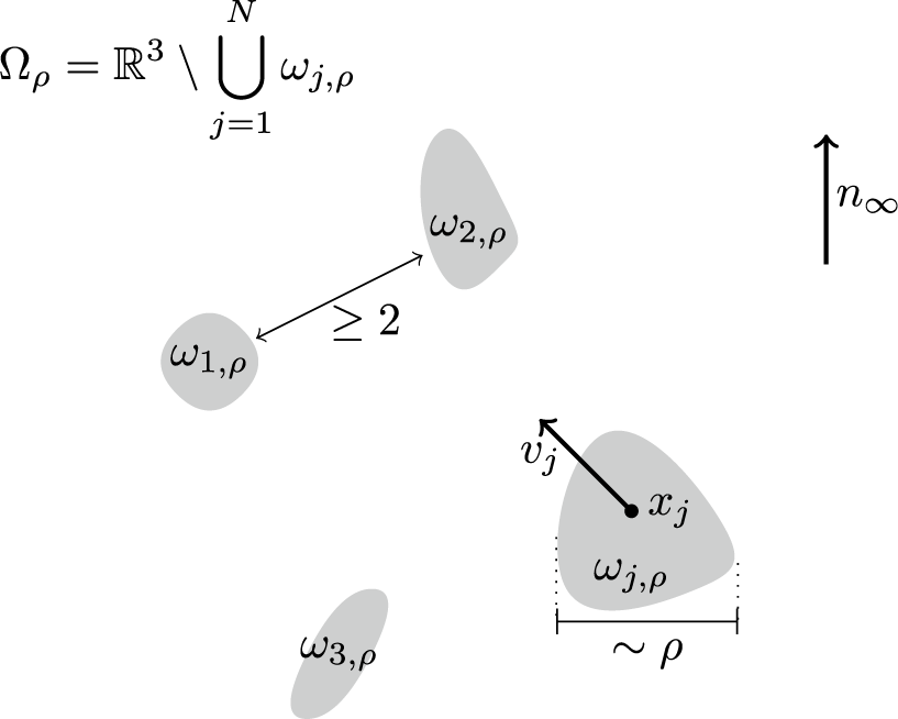
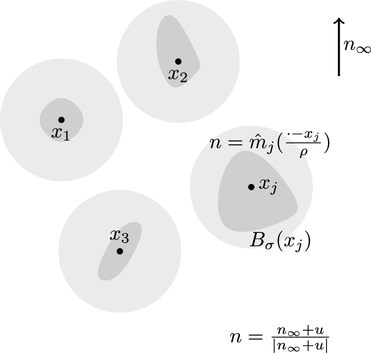

 Open access