


1. Introduction
Pulsars are highly magnetised, rotating, dense, and compact stars observed to have periodic radiation of pulses with the periodicity tied to their remarkably stable rotation. The slowdown in the rotation of a pulsar is influenced by two types of instabilities: glitches and timing noise (D’alessandro Reference D’alessandro1996; Haskell & Melatos Reference Haskell and Melatos2015; Zhou et al. 2022). Glitches are abrupt changes in the rotational frequency and spin-down rate of a pulsar, while timing noise is a stochastic wander in the spin parameters of pulsars. The occurrence of glitches, as well as their slow relaxations, which range from a few days to several years, reveals the presence of neutron superfluidity within the inner crust of the neutron star. One of the most widely accepted mechanisms for explaining glitches and their recoveries is the superfluid vortex pinning and creep model (Anderson & Itoh Reference Anderson and Itoh1975; Alpar et al. Reference Alpar, Pines, Anderson and Shaham1984b; Alpar, Langer, & Sauls Reference Alpar, Langer and Sauls1984a). This model suggests that neutron superfluidity in the interior of the star leads to a differential rotation, storing a significant amount of angular momentum. When this angular momentum is released, the crust spins up, resulting in a glitch. Pulsar glitches thus provide valuable insights into the superfluid dynamics within the star (Zhou et al. Reference Zhou2022; Liu et al. Reference Liu2024).
The post-glitch recovery is the process in which the pulsar gradually relaxes back towards its original pre-glitch rotational state. According to the vortex creep model, this process is driven by the repinning of superfluid vortices to the crustal nuclei and the re-establishment of the equilibrium lag between the rotational rates of the superfluid interior and the crust. The specific timescale and form of the relaxation, whether exponential or linear, are determined by the distinct vortex dynamics at play. While the standard recovery reflects the transfer of angular momentum from the interior to the surface, deviations from this norm can indicate complex interactions, such as crustal events or non-linear creep regimes (Akbal et al. Reference Akbal, Gügercinoğlu, Sasmaz Mus and Alpar2015; Gügercinoğlu, Köksal, & Güver 2023). Ultimately, the post-glitch recovery serves as a probe for the internal dynamics and structure of neutron stars (Gügercinoğlu et al. 2022).
PSR J0835–4510, B0833–45, the Vela pulsar, has 26 reported glitch events, most of which are large glitches and detected after a regular, quasi-periodic inter-glitch timeFootnote
a
(Espinoza et al. Reference Espinoza, Lyne, Stappers and Kramer2011; Basu et al. Reference Basu2022). The Vela pulsar is one of the most studied glitching pulsars. The first-ever glitch was recorded in the Vela pulsar (Radhakrishnan & Manchester Reference Radhakrishnan and Manchester1969; Reichley & Downs Reference Reichley and Downs1969). Moreover, the first-ever glitch detected in real time was also observed in the Vela pulsar (Palfreyman et al. Reference Palfreyman, Dickey, Hotan, Ellingsen and van Straten2018). The Vela pulsar is considered one of the most popular glitching pulsars for several reasons: it is a bright, young source that displays glitches at regular intervals. The recoveries of glitches also demonstrate strikingly similar behaviour. A measure of a pulsar’s slowdown over time is described by the braking index (n). It is defined by a power-law relation between the pulsar’s spin-down rate $\dot{\Omega}$
and its rotational angular frequency (
$\dot{\Omega}$
and its rotational angular frequency ( $\Omega$
), given by
$\Omega$
), given by $\dot{\Omega} = k \Omega^n$
. The braking index provides insights into the pulsar’s rotational evolution, magnetic fields, and emission mechanisms.
$\dot{\Omega} = k \Omega^n$
. The braking index provides insights into the pulsar’s rotational evolution, magnetic fields, and emission mechanisms.
Here, we present the observational behaviour of the Vela pulsar from September 2016 to January 2025; during this period, four large glitches were observed in our monitoring campaign (Grover et al. Reference Grover2024b; Basu et al. Reference Basu2020). Theoretical inferences from the post-glitch recovery phase are also presented. We have used the recovery behaviour of four glitches in the Vela pulsar to estimate the following parameters: (a) the fractional moments of inertia (FMI) of various layers participating in a glitch, (b) the re-coupling timescale of the crustal superfluid, (c) theoretical prediction for the time to the next glitch, (d) braking index of the Vela pulsar. The paper’s outline is as follows: a brief description of the vortex creep and bending models is given in Section 2. We describe the pulsar observations, the data reduction, and the analysis processes in Section 3. In Section 4, we present the results. The conclusions and future scope are given in Section 5.
2. The vortex creep and bending models
The vortex creep model provides a microscopic framework for understanding the macroscopic behaviour of glitches and their subsequent recovery. In the neutron star crust, vortex lines coexist with and energetically pin to the crystal lattice. Crustal inhomogeneities such as dislocations, cracks, and impurities produced by quakes create a non-uniform vortex distribution known as vortex traps (Cheng et al. Reference Cheng, Alpar, Pines and Shaham1988). Glitches may arise due to collective vortex unpinning events induced in these vortex traps when the angular velocity lag between the superfluid and the crustal normal matter exceeds a threshold value (Anderson & Itoh Reference Anderson and Itoh1975; Alpar et al. Reference Alpar, Pines, Anderson and Shaham1984b). During the unpinning events, angular momentum is rapidly transferred from the superfluid to the crust. The superfluid regions involved in the unpinning decouple from the external braking torque, resulting in a step increase in the spin-down rate.
After a glitch, the steady-state lag decreases, temporarily suppressing creep in some superfluid regions. The recovery process involves restoring the creep until steady-state conditions are re-established by the external braking torque. Shortly after the glitch, excess angular momentum is transferred from the crustal superfluid to the normal matter in the crust, producing a transient peak in the crustal rotation rate. This perturbation is subsequently communicated to the core superfluid through electron scattering off magnetised vortex lines (Alpar et al. Reference Alpar, Langer and Sauls1984a), causing the initial peak to relax on the crust–core coupling timescale toward a new equilibrium state. A pronounced peak in the rotation rate of the normal component is expected when the coupling between the crustal superfluid and the normal matter is stronger than that with the core superfluid (Pizzochero, Montoli, & Antonelli Reference Pizzochero, Montoli and Antonelli2020). On longer timescales, the core superfluid recouples, leaving only the crustal superfluid effectively decoupled from the external braking torque.
In some glitches of the Crab pulsar, delayed spin-ups are observed (Wong, Backer, & Lyne Reference Wong, Backer and Lyne2001; Shaw et al. Reference Shaw2018; Basu et al. Reference Basu2020; Ge et al. Reference Ge2020). Within the vortex creep framework, these features are attributed to vortex unpinning accompanied by inward vortex motion driven by fractured crustal platelets (Akbal et al. Reference Akbal, Gügercinoğlu, Sasmaz Mus and Alpar2015; Gügercinoğlu & Alpar 2019). Additionally, damped, sinusoidal-like oscillations in the spin-down rate can arise from vortex-line bending in the non-linear creep relaxation regime, excited by the glitch and may also be influenced by preceding glitch events (Gügercinoğlu et al. 2023). It is important to note that the vortex creep model is not the unique explanation; several equally viable models successfully explain glitch-triggering mechanisms, delayed spin-ups, and post-glitch relaxation. For a comprehensive discussion, see Haskell & Melatos (Reference Haskell and Melatos2015), Antonopoulou, Haskell, & Espinoza (Reference Antonopoulou, Haskell and Espinoza2022), Antonelli, Montoli, & Pizzochero (Reference Antonelli, Montoli, Pizzochero and Vasconcellos2022), Zhou et al. (Reference Zhou2022).
The post-glitch spin-down rate behaviour mirrors the responses of the vortex creep regions in both linear and non-linear regimes to a glitch, with additional involvement of induced inward vortex motion in delayed spin-up events (Akbal et al. Reference Akbal, Gügercinoğlu, Sasmaz Mus and Alpar2015). In certain regions of the superfluid in the inner crust and the outer core, vortex creep exhibits a linear response to glitch-induced changes, leading to exponential relaxation (Alpar et al. Reference Alpar, Cheng and Pines1989; Flanagan Reference Flanagan1990; Gügercinoğlu 2017) as:
 \begin{equation} \Delta \dot{\nu}(t) = \sum_{i=1}^{3} - \frac{I_{\text{ei}}}{I_{{c}}} \frac{\Delta \nu}{\tau_{\text{ei}}} e^{-t / \tau_{\text{ei}}},\end{equation}
where $\Delta \nu = \nu - \nu_0$
,
$\Delta \nu = \nu - \nu_0$
, $\nu$
is the spin frequency,
$\nu$
is the spin frequency, $\nu_0$
is the spin frequency just before the glitch,
$\nu_0$
is the spin frequency just before the glitch, $I_{\text{ei}}/ I_{c}$
is the FMI of the of ith layer that participated in a glitch, and
$I_{\text{ei}}/ I_{c}$
is the FMI of the of ith layer that participated in a glitch, and $\tau_{\text{ei}}$
is the corresponding exponential recovery timescale.
$\tau_{\text{ei}}$
is the corresponding exponential recovery timescale.
The overall linear relaxation, obtained by integrating the contributions of several neighbouring single non-linear regime regions (Alpar et al. Reference Alpar, Pines, Anderson and Shaham1984b; Gügercinoğlu et al. 2022), with an assumption of linearly decreasing superfluid angular velocity during a glitch (Alpar et al. Reference Alpar, Chau, Cheng and Pines1996) and is given as:
 \begin{equation} \Delta \dot{\nu}(t) = \frac{I_{{a}}}{I_{{c}}} \dot{\nu}_0 \left[1 - \frac{1- (\tau_{\text{nl}} / t_0) \text{ln}[1+({e}^{t_0/ \tau_{\text{nl}}} - 1){e}^{-t/ \tau_{\text{nl}}}]}{1-{e}^{-t/ \tau_{\text{nl}}}} \right],\end{equation}
where $\dot{\nu}_0$
spin-down rate just before the glitch,
$\dot{\nu}_0$
spin-down rate just before the glitch, $I_{a}/ I_{c}$
is the FMI of the non-linear crustal superfluid region,
$I_{a}/ I_{c}$
is the FMI of the non-linear crustal superfluid region, $t_0$
is the offset time, and
$t_0$
is the offset time, and $\tau_{\text{nl}}$
is the non-linear creep relaxation time. The non-linear creep response gives an estimate for the time to the next glitch. The glitch-induced changes in the spin-down rate fully relax after a waiting time (Gügercinoğlu et al. 2022),
$\tau_{\text{nl}}$
is the non-linear creep relaxation time. The non-linear creep response gives an estimate for the time to the next glitch. The glitch-induced changes in the spin-down rate fully relax after a waiting time (Gügercinoğlu et al. 2022),
 \begin{equation} t_0 = \frac{\delta\nu_{s} + \Delta\nu_{c}}{|\dot{\nu}|} \cong \frac{\delta\nu_{s}}{|\dot{\nu}|}.\end{equation}
where $\Delta\nu_{c}$
is the observed glitch magnitude and
$\Delta\nu_{c}$
is the observed glitch magnitude and $\delta\nu_{s}$
represents the decrement in the superfluid rotational frequency. The post-glitch recovery completes once the relaxation of the non-linear creep regions is finished. This gives us a theoretical prediction for the time to the next glitch in terms of the vortex creep model, which lies between the range
$\delta\nu_{s}$
represents the decrement in the superfluid rotational frequency. The post-glitch recovery completes once the relaxation of the non-linear creep regions is finished. This gives us a theoretical prediction for the time to the next glitch in terms of the vortex creep model, which lies between the range $t_0-3\tau_{\mathrm{nl}}$
to
$t_0-3\tau_{\mathrm{nl}}$
to $t_0+3\tau_{\mathrm{nl}}$
.
$t_0+3\tau_{\mathrm{nl}}$
.
A typical post-glitch recovery involves an exponential and a linear relaxation described by equations (1) and (2), respectively. This is tested by using different alternative models as described below:
-
• Model 1: Only exponential recovery given by equation (1).
-
− Model 1a: Exponential recovery with only 1 exponential component.
-
− Model 1b: Exponential recovery with 2 exponential components.
-
− Model 1c: Exponential recovery with 3 exponential components.
-
-
• Model 2: Only linear relaxation described by equation (2).
-
• Model 3: Exponential and linear recoveries, the sum of equations (1) and (2).
-
− Model 3a: The sum of linear recovery and exponential recovery with only 1 exponential component.
-
− Model 3b: The sum of linear recovery and exponential recovery with 2 exponential components.
-
− Model 3c: The sum of linear recovery and exponential recovery with 3 exponential components.
-
The most preferred model and corresponding parameters among the various alternatives were evaluated using Bayesian analysis of our post-glitch recovery measurements of the Vela pulsar. Further details of this analysis are presented in the next section.
Apart from long-term post-glitch recovery, we see evidence for sinusoidal-like spin-down rate oscillations over and above the recovery predicted by the vortex creep model as described in Section 4. Such oscillations can be explained by vortex bending (Gügercinoğlu et al. 2023) and appear to be a common feature following glitches, as also observed from PSRs J1522–5735 (Zhou et al. Reference Zhou2024), J0742–2822 (Zubieta et al. Reference Zubieta2025a), J1509–5850, and J1718–3825 (Liu et al. Reference Liu2025). To understand this better, we used three alternative hypotheses as described below
-
• Hypothesis I – An undamped model consisting of only sinusoidal term, $A\sin (\omega t+\phi)$
.
$A\sin (\omega t+\phi)$
. -
• Hypothesis II – Damped model consisting of a sinusoidal term and a damping factor,
$A\sin (\omega t+\phi) \exp(\!-t/\tau)$
. -
• Hypothesis III – An oscillatory model as described in Gügercinoğlu et al. (2023) consisting of
$A\omega\cos(\omega t+\phi)\exp(\!-t/2\tau)-(A/2\tau) \sin(\omega t+\phi) \exp(\!-t/2\tau)$
,


where A is the amplitude, $\omega$
is the angular frequency,
$\omega$
is the angular frequency, $\phi$
is the phase, and
$\phi$
is the phase, and $\tau$
is the decay time for the oscillation. The next section outlines the observations, data reduction, and timing analysis used to derive the spin frequency and spin-down rate. It also describes the Bayesian analysis used to calculate the evidence for the competing hypotheses, thereby identifying the most plausible model and estimating its corresponding parameters.
$\tau$
is the decay time for the oscillation. The next section outlines the observations, data reduction, and timing analysis used to derive the spin frequency and spin-down rate. It also describes the Bayesian analysis used to calculate the evidence for the competing hypotheses, thereby identifying the most plausible model and estimating its corresponding parameters.
3. Observations and analysis
3.1. Sample and observational facilities
We use two large radio telescopes to monitor pulsars: the upgraded Giant Metrewave Radio Telescope (uGMRT)(Gupta et al. Reference Gupta2017) and the Ooty Radio Telescope (ORT) (Swarup et al. Reference Swarup1971). Observations of PSR B0833 $-$
45 were part of a regular glitch monitoring program, where we regularly monitor 24 pulsars (i) to detect glitches, (ii) model timing noise, and (iii) model post-glitch recovery. This work presents a comprehensive analysis of the Vela pulsar’s rotational evolution, spanning from September 2016 to January 2025, as part of our ongoing monitoring campaign (Grover et al. Reference Grover2024b; Basu et al. Reference Basu2020). Our study primarily uses observations from the ORT, supplemented by uGMRT and archival ATNF data to fill temporal gaps and facilitate specialised investigations.
$-$
45 were part of a regular glitch monitoring program, where we regularly monitor 24 pulsars (i) to detect glitches, (ii) model timing noise, and (iii) model post-glitch recovery. This work presents a comprehensive analysis of the Vela pulsar’s rotational evolution, spanning from September 2016 to January 2025, as part of our ongoing monitoring campaign (Grover et al. Reference Grover2024b; Basu et al. Reference Basu2020). Our study primarily uses observations from the ORT, supplemented by uGMRT and archival ATNF data to fill temporal gaps and facilitate specialised investigations.
The ORT (Swarup et al. Reference Swarup1971) is a 530 m $\times$
30 m parabolic cylindrical reflector. It is located on a hill with the same slope as the geographic latitude (11
$\times$
30 m parabolic cylindrical reflector. It is located on a hill with the same slope as the geographic latitude (11 $^{\circ}$
), allowing it to track sources for about 8 h and covers a declination range of
$^{\circ}$
), allowing it to track sources for about 8 h and covers a declination range of $-60$
$-60$ $^{\circ}$
to
$^{\circ}$
to $+60$
$+60$ $^{\circ}$
. Pulsar observations at the ORT are carried out at the central observation frequency of 326.5 MHz using the Pulsar Ooty Radio Telescope’s New Digital Efficient Receiver, PONDER (Naidu et al. Reference Naidu, Joshi, Manoharan and Krishnakumar2015), which produces real-time coherent dedispersed time series data. The typical cadence of the observations at the ORT is 1–14 d.
$^{\circ}$
. Pulsar observations at the ORT are carried out at the central observation frequency of 326.5 MHz using the Pulsar Ooty Radio Telescope’s New Digital Efficient Receiver, PONDER (Naidu et al. Reference Naidu, Joshi, Manoharan and Krishnakumar2015), which produces real-time coherent dedispersed time series data. The typical cadence of the observations at the ORT is 1–14 d.
The GMRT is an interferometer with 30 parabolic antennas, with a diameter of 45 m each (Swarup et al. Reference Swarup1991; Ananthakrishnan Reference Ananthakrishnan1995). The uGMRT (Gupta et al. Reference Gupta2017) covers a declination range of $-53^{\circ}$
to
$-53^{\circ}$
to $+90^{\circ}$
and supports observations from 150 to 1 460 MHz in four bands. The Vela pulsar is observed in uGMRT Band 3 (250–500 MHz) and Band 4 (550–950 MHz). The central square antennas, together with a subset of the nearest arm antennas, were used in a phased array to synthesise a large single dish for observations. The outer arm antennas were not included in the phased array due to significant drift in the phase of the voltage outputs, caused by ionospheric variations, in these antennas. A digital filterbank, implemented in the GMRT correlator, was used to record either 1 024 or 2 048 channels across the bandpass to obtain frequency-resolved data with a typical sampling time of 655
$+90^{\circ}$
and supports observations from 150 to 1 460 MHz in four bands. The Vela pulsar is observed in uGMRT Band 3 (250–500 MHz) and Band 4 (550–950 MHz). The central square antennas, together with a subset of the nearest arm antennas, were used in a phased array to synthesise a large single dish for observations. The outer arm antennas were not included in the phased array due to significant drift in the phase of the voltage outputs, caused by ionospheric variations, in these antennas. A digital filterbank, implemented in the GMRT correlator, was used to record either 1 024 or 2 048 channels across the bandpass to obtain frequency-resolved data with a typical sampling time of 655 $\mu$
s. The cadence of the observations is 15–30 d. We primarily use frequency-resolved uGMRT data to examine the impact of dispersion measure (DM) offsets on the spin-down rate. Additionally, the uGMRT data filled a temporal gap around epoch 60 300, providing crucial estimates not covered by ORT due to maintenance downtime.
$\mu$
s. The cadence of the observations is 15–30 d. We primarily use frequency-resolved uGMRT data to examine the impact of dispersion measure (DM) offsets on the spin-down rate. Additionally, the uGMRT data filled a temporal gap around epoch 60 300, providing crucial estimates not covered by ORT due to maintenance downtime.
The Commonwealth Scientific and Industrial Research Organisation (CSIRO) Data Access Portal is used to access the Parkes pulsar archival observationsFootnote b (Hobbs et al. Reference Hobbs2011) of the Vela pulsar. These data were mainly used to fill temporal gaps in glitch number 2 (MJD 58515), that were not covered by observations with the ORT and uGMRT. We directly downloaded and used the reduced files (or PSRFITS: Hotan, van Straten, & Manchester Reference Hotan, van Straten and Manchester2004) and performed subsequent analysis, as described in the next subsection.
The rotational evolution of the Vela pulsar from September 2016 to January 2025.

3.2. Data reduction and timing analysis
We used the DSPSR software (van Straten & Bailes Reference van Straten and Bailes2011) and the PINTA pipeline (Susobhanan et al. Reference Susobhanan2021) to reduce the raw data from the Vela pulsar observed at the ORT and the uGMRT, respectively, into PSRFITS files, using the ephemeris created in our initial observations. The initial analysis, including the generation of a noise-free template and Time of Arrivals (ToAs), was performed using PSRCHIVE (Hotan et al. Reference Hotan, van Straten and Manchester2004; van Straten, Demorest, & Oslowski Reference van Straten, Demorest and Oslowski2012). The ToAs were obtained through the cross-correlation of the template profile with all other observed profiles using the ‘pat’ command, using the Fourier Phase Gradient (PGS) method (Taylor Reference Taylor1992). The precision timing analysis of the pulsar was done with the help of the pulsar timing software TEMPO2 (Hobbs, Edwards, & Manchester Reference Hobbs, Edwards and Manchester2006; Edwards, Hobbs, & Manchester Reference Edwards, Hobbs and Manchester2006). The DM offsets were estimated using the DMcalc (Krishnakumar et al. Reference Krishnakumar2021) script from the frequency-resolved data from uGMRT. The rotational evolution of a pulsar including a glitch can be expressed as a Taylor series expansion (Gügercinoğlu et al. 2022),
 \begin{align} \nu(t) = & \nu_0 + \dot{\nu}_0(t-t_0) + \frac{1}{2} \ddot{\nu}_0(t-t_0)^2 + \Delta \nu_g \nonumber\\[3pt] & + \Delta \dot{\nu}_g(t-t_g) + \Delta \nu_d \exp(\!-(t-t_g)/\tau_d) \ , \\[-10pt] \nonumber \end{align}
where $\nu_0$
is the spin frequency, and
$\nu_0$
is the spin frequency, and $\dot{\nu}_0$
and
$\dot{\nu}_0$
and $\ddot{\nu}_0$
are the first and second derivatives of the frequency, respectively, at reference epoch
$\ddot{\nu}_0$
are the first and second derivatives of the frequency, respectively, at reference epoch $t_0$
.
$t_0$
. $\Delta \nu_g$
and
$\Delta \nu_g$
and $\Delta \dot{\nu}_g(t-t_g)$
denote the changes in spin frequency and its first derivative at the glitch epoch
$\Delta \dot{\nu}_g(t-t_g)$
denote the changes in spin frequency and its first derivative at the glitch epoch $t_g$
, respectively. The parameters
$t_g$
, respectively. The parameters $\Delta \nu_d$
and
$\Delta \nu_d$
and $\tau_d$
correspond to the amplitude and characteristic decay timescale of the exponential relaxation component following the glitch.
$\tau_d$
correspond to the amplitude and characteristic decay timescale of the exponential relaxation component following the glitch.
The spin evolution of the Vela pulsar from September 2016 to January 2025, obtained after precision timing, is given in Figure 1. Each measurement is made with the local timing of several epochs, typically within a 50–200 d data window, contingent on data availability. Exceptions include the first and last few points adjacent to glitches. The resulting measurements are reflected in the precision of error bars, which are smaller than the symbol used in the figure. By choosing multi-epoch windows, we achieve reliable rotational estimates with minimised error bars, providing a robust foundation for studying vortex residuals. This approach effectively averages out temporal effects caused by physical processes, such as ionised interstellar medium scattering-induced broadening, thereby validating the accuracy of measurements aligned with the star’s rotation and internal dynamics. These recovery measurements are investigated within the framework of the vortex creep and bending models as described in Section 2 and the results are discussed in Section 4.
3.3. Bayesian analysis
For each recovery, we used Bayesian statistics for model comparison and parameter estimation. Bayesian statistics use Bayes’ theorem to enhance the probability of a hypothesis based on new evidence or data. We used DYNESTY (a dynamic nested sampling package for estimating Bayesian posteriors and evidences; Speagle Reference Speagle2020) to compute the Bayesian evidence and perform model selection, and EMCEE (Foreman-Mackey et al. Reference Foreman-Mackey, Hogg, Lang and Goodman2013) to obtain posterior samples for parameter estimation of the preferred model. For model comparison, the standard Jeffreys scale is used, which suggests the preferred model based on the strength of evidence (Trotta Reference Trotta2008). Bayesian inference is also used to predict the epoch of the next glitch using data from previous glitches.
The priors are selected based on the initial knowledge of each parameter, as informed by the literature (Gügercinoğlu et al. 2022; Flanagan Reference Flanagan1990; Alpar et al. Reference Alpar, Cheng and Pines1989). This knowledge provides reasonable initial ranges that were further refined or broadened based on the results. For instance, parameters such as the fractional moment of inertia ( $I_{e}/I$
or
$I_{e}/I$
or $I_{a}/I$
) is generally positive and below unity. The recoupling timescale in exponential regions (
$I_{a}/I$
) is generally positive and below unity. The recoupling timescale in exponential regions ( $\tau_{e}$
) depends on the number of exponential components (three-, two-, or one-component models). Typically, for the Vela pulsar, it has been observed that the first component lies within 0.1–10 d, with the second and third components approximately 10 and 100 times longer, respectively.
$\tau_{e}$
) depends on the number of exponential components (three-, two-, or one-component models). Typically, for the Vela pulsar, it has been observed that the first component lies within 0.1–10 d, with the second and third components approximately 10 and 100 times longer, respectively.
For the linear relaxation region, the prior for recoupling timescale ( $\tau_{\mathrm{nl}}$
) is around 10–300 d, and the offset time (
$\tau_{\mathrm{nl}}$
) is around 10–300 d, and the offset time ( $t_0$
) is 300–1 200, with the initial guess often chosen close to the observed time to the next glitch. For the Vortex bending studies, the prior on amplitude, phase, and decay constant were set as 0–1, 0–2
$t_0$
) is 300–1 200, with the initial guess often chosen close to the observed time to the next glitch. For the Vortex bending studies, the prior on amplitude, phase, and decay constant were set as 0–1, 0–2 $\pi$
, and 0–2 000 d, respectively. All the priors were considered as uniform priors and listed in Table 1. While these priors adequately describe many recoveries, particularly those observed in the Vela pulsar, their applicability may vary depending on the nature of the recovery. As each recovery exhibits unique characteristics, a flexible and adaptive approach to defining priors is essential. We model the data assuming independent Gaussian measurement uncertainties. The corresponding log-likelihood function is given by
$\pi$
, and 0–2 000 d, respectively. All the priors were considered as uniform priors and listed in Table 1. While these priors adequately describe many recoveries, particularly those observed in the Vela pulsar, their applicability may vary depending on the nature of the recovery. As each recovery exhibits unique characteristics, a flexible and adaptive approach to defining priors is essential. We model the data assuming independent Gaussian measurement uncertainties. The corresponding log-likelihood function is given by
 \begin{equation}\ln \mathcal{L}(\boldsymbol{\theta}) = -\frac{1}{2}\sum_{i}\left[\frac{\left(d_i - m_i(\boldsymbol{\theta})\right)^2}{\unicode{x03C3}_i^2}+ \ln\left(2\pi \unicode{x03C3}_i^2\right)\right],\end{equation}
where $d_i$
denotes the observed data,
$d_i$
denotes the observed data, $m_i(\boldsymbol{\theta})$
is the model prediction for parameters
$m_i(\boldsymbol{\theta})$
is the model prediction for parameters $\boldsymbol{\theta}$
, and
$\boldsymbol{\theta}$
, and $\unicode{x03C3}_i$
represents the corresponding measurement uncertainty.
$\unicode{x03C3}_i$
represents the corresponding measurement uncertainty.
Prior ranges used for the parameter estimation of each recovery. The left column represents the parameter, and the right column displays the values with their corresponding units. The symbols $I_{e1}/I$
,
$I_{e1}/I$
, $\tau_{e1}$
,
$\tau_{e1}$
, $I_{e2}/I$
,
$I_{e2}/I$
, $\tau_{e2}$
,
$\tau_{e2}$
, $I_{e3}/I$
,
$I_{e3}/I$
, $\tau_{e3}$
represent the fractional moment of inertia and the decay timescales for the first, second and third components of exponential recovery, respectively.
$\tau_{e3}$
represent the fractional moment of inertia and the decay timescales for the first, second and third components of exponential recovery, respectively. $I_{a}/I$
,
$I_{a}/I$
, $\tau_{\mathrm{nl}}$
,
$\tau_{\mathrm{nl}}$
, $t_0$
denote the fractional moment of inertia, the decay timescales, and offset time associated with the linear relaxation, respectively. And A is the amplitude,
$t_0$
denote the fractional moment of inertia, the decay timescales, and offset time associated with the linear relaxation, respectively. And A is the amplitude, $\phi$
is the phase, and
$\phi$
is the phase, and $\tau$
is the exponential decay constant for oscillations.
$\tau$
is the exponential decay constant for oscillations.

The post-glitch recoveries are studied within the framework of the vortex creep model and the vortex bending model (Gügercinoğlu et al. 2023), discussed in the previous section. A quick picture of the analysis process is as follows: we first model the frequency derivative measurements from the data using the vortex creep model. Then, we estimate the vortex residuals obtained by subtracting the vortex creep model's predictions from the observational data. These vortex residuals were investigated within the framework of the vortex bending model. The generalised Lomb-Scargle periodogram technique (Lomb Reference Lomb1976; Scargle Reference Scargle1982; VanderPlas 2018) was employed to detect periodicities in the vortex residuals. We used the Astropy (Astropy Collaboration et al. 2013) implementation of the generalised Lomb-Scargle periodogram. The Peaks with false alarm probabilities (FAP) below 0.1% or Z-score above 3 $\unicode{x03C3}$
were considered significant for vortex bending studies. FAP estimation was performed using the Baluev (Reference Baluev2008) method. Alternative methods, including approximations based on effective independent frequencies and bootstrap resampling, yielded similar results. The significance of each detected peak is quantified using the Lomb–Scargle false-alarm probability (FAP). For interpretive purposes, we also report the equivalent Z-score values (Cowan et al. Reference Cowan, Cranmer, Gross and Vitells2011; Ganguly & Desai Reference Ganguly and Desai2017). The results of our analysis are presented in the next section.
$\unicode{x03C3}$
were considered significant for vortex bending studies. FAP estimation was performed using the Baluev (Reference Baluev2008) method. Alternative methods, including approximations based on effective independent frequencies and bootstrap resampling, yielded similar results. The significance of each detected peak is quantified using the Lomb–Scargle false-alarm probability (FAP). For interpretive purposes, we also report the equivalent Z-score values (Cowan et al. Reference Cowan, Cranmer, Gross and Vitells2011; Ganguly & Desai Reference Ganguly and Desai2017). The results of our analysis are presented in the next section.
4. Results and discussions
Our pulsar monitoring program with the ORT and the uGMRT started in 2015. The previous results were reported in Basu et al. (Reference Basu2020) and Grover et al. (Reference Grover2024b). In this work, we present an analysis of a new Vela glitch at MJD 60429.9. Further, we demonstrate the spin-down rate evolution for the Vela pulsar since the beginning of the monitoring program. Our primary focus is to provide the theoretical interpretation of glitches using the post-glitch recovery phase and to obtain measurements for the re-coupling timescales and fractional moment of inertia for various layers that participate in a glitch. We have estimated the theoretical time to the next glitch through the vortex creep model and used Bayesian inference to predict the time for the next glitch. All the predictions match well with the observed inter-glitch times.
4.1. Glitches
Here, we summarise the last three glitches in the Vela pulsar: MJD 57734.4, 58517, and 59417.6, detected in our monitoring program (Grover et al. Reference Grover2024b; Basu et al. Reference Basu2020). The recoveries for each of these glitches are studied within the framework of the vortex creep model to investigate the structure of the Vela pulsar. Furthermore, we report the detection and analysis of the recent large glitch in the Vela pulsar in 2024. The characteristics and parameters of glitches are listed in Table 2.
Glitches in the Vela pulsar detected in our monitoring program. The columns from left to right represent the glitch number, glitch epoch, pre-glitch spin frequency, pre-glitch spin-down rate, fractional change in spin frequency (glitch magnitude), and fractional change in the spin-down rate and the reference.

The parameters estimated by fitting the vortex creep model to the observed post-glitch recovery data for the last four glitches in the Vela pulsar. The first column represents the glitch epoch. Columns 2–7 represent the fractional moment of inertia, and corresponding decay timescales with 95% credible intervals for the first, second, and third exponential recovery components (equation 1), respectively. Columns 8 and 9 provide the fractional moment of inertia for linear recovery and the recoupling timescale with 95% credible intervals, respectively. The offset time with a 95% credible interval is given in column 10 (equation 2). The observed inter-glitch interval is given in column 11, and column 12 contains the predicted inter-glitch time using MCMC sampling with a 68% credible interval.

We present the parameters of the Vela 2024 glitch, which occurred around MJD 60429.9. This glitch has been reported by several groups (Zubieta et al. Reference Zubieta2024; Campbell-Wilson, Flynn, &Bateman Reference Campbell-Wilson, Flynn and Bateman2024; Grover et al. Reference Grover, Krishnakumar, Joshi and Arumugam2024a; Palfreyman Reference Palfreyman2024;Wang et al. Reference Wang2024; Zubieta et al. Reference Zubieta2025b). Here, we present updates in our preliminary results reported in Grover et al. (Reference Grover, Krishnakumar, Joshi and Arumugam2024a). The glitch is estimated to occur at MJD 60429.9(1), with the fractional increase in the spin frequency, and its time derivative is calculated as $2\,396(2)\times10^{-9}$
and
$2\,396(2)\times10^{-9}$
and $23(1)\times10^{-3}$
, respectively. The results of the glitch epoch and spin parameters agree with the reported estimates of other monitoring programs. A more precise measurement of glitch epoch as 60429.86962(4) is also presented in Palfreyman (Reference Palfreyman2024) with higher cadence observations. The timing residuals, the evolution of the spin frequency, and the spin-down rate are given in Figure 2. The post-glitch recovery for this glitch is also investigated within the framework of the vortex creep model in the next subsection.
$23(1)\times10^{-3}$
, respectively. The results of the glitch epoch and spin parameters agree with the reported estimates of other monitoring programs. A more precise measurement of glitch epoch as 60429.86962(4) is also presented in Palfreyman (Reference Palfreyman2024) with higher cadence observations. The timing residuals, the evolution of the spin frequency, and the spin-down rate are given in Figure 2. The post-glitch recovery for this glitch is also investigated within the framework of the vortex creep model in the next subsection.
Glitch observed in PSR J0835–4510 on MJD 60429.9. The top panel represents the timing residuals. The middle and bottom panels display the evolution of $\Delta \nu$
and
$\Delta \nu$
and $\Delta \dot\nu$
, respectively. The vertical dashed line indicates the glitch epoch.
$\Delta \dot\nu$
, respectively. The vertical dashed line indicates the glitch epoch.

4.2. Post-glitch recoveries
In this section, we present the post-glitch recovery behaviour of the Vela pulsar. The spin-down rate has been analysed from MJD 57651 to 60700. During this period, the Vela pulsar has displayed four glitches. The post-glitch recovery of the Vela pulsar is regular, i.e. it follows similar behaviour. The recovery for this pulsar usually consists of exponential and linear relaxations well described by Model 3 in Section 2. We have investigated all post-glitch recoveries for this pulsar within the framework of the vortex creep model for the glitches listed in Table 2, and the resulting fit parameters obtained using the vortex creep model are listed in Table 3. Now, we concisely describe the post-glitch relaxation(s) for individual cases.
The post-glitch recovery of the Vela glitch G1. The top panel shows the observed change in the spin-down rate relative to the pre-glitch spin-down rate (blue dots) and the best-fit vortex creep model predictions (red solid curve). The bottom panel displays the residuals obtained by subtracting the best-fit values from the measurements of the spin-down rate on the scale of $10^{-11}$
Hz s
$10^{-11}$
Hz s $^{-1}$
.
$^{-1}$
.

4.2.1. Glitch No. 1 – MJD 57734.4(2)
G1, or glitch at MJD 57734.4(2) (Sarkissian et al. Reference Sarkissian, Reynolds, Hobbs and Harvey-Smith2017; Palfreyman et al. Reference Palfreyman, Dickey, Hotan, Ellingsen and van Straten2018; Ashton et al. Reference Ashton, Lasky, Graber and Palfreyman2019; Basu et al. Reference Basu2020; Gügercinoğlu & Alpar 2020; Montoli et al. Reference Montoli, Antonelli, Magistrelli and Pizzochero2020; Dunn et al. Reference Dunn2025), was detected with a fractional change in the rotational frequency of 1 433(1) $\times 10^{-9}$
, and a fractional change in the spin-down rate as 5.59(1)
$\times 10^{-9}$
, and a fractional change in the spin-down rate as 5.59(1) $\times 10^{-3}$
. We present the post-glitch relaxation modelling for this glitch in Figure 3. For this recovery, the Bayesian model comparison prefers the presence of three-exponential + linear recovery (Model 3c) over all other models. The estimated median values for parameters are: the fractional moment of inertia for the first, second, and third exponential components are
$\times 10^{-3}$
. We present the post-glitch relaxation modelling for this glitch in Figure 3. For this recovery, the Bayesian model comparison prefers the presence of three-exponential + linear recovery (Model 3c) over all other models. The estimated median values for parameters are: the fractional moment of inertia for the first, second, and third exponential components are $4.5 \times 10^{-3}$
,
$4.5 \times 10^{-3}$
, $3.9 \times 10^{-3}$
and
$3.9 \times 10^{-3}$
and $58.4 \times 10^{-3}$
respectively, with the decay timescales of
$58.4 \times 10^{-3}$
respectively, with the decay timescales of $4.9$
,
$4.9$
, $29.3$
and
$29.3$
and $298.5$
d, respectively. The median fractional moment of inertia for the non-linear creep region is
$298.5$
d, respectively. The median fractional moment of inertia for the non-linear creep region is $4.4 \times 10^{-3}$
with a recoupling timescale of 62 d. The offset time is measured as
$4.4 \times 10^{-3}$
with a recoupling timescale of 62 d. The offset time is measured as $774.0$
d, close to the observed inter-glitch time of 783 d. The observed time is consistent with the vortex creep model’s predicted range and closely matches the Bayesian prediction, which estimates a 68% credible interval of 787–1 083 d. The fit parameters, along with their 95% credible intervals, are listed in Table 3.
$774.0$
d, close to the observed inter-glitch time of 783 d. The observed time is consistent with the vortex creep model’s predicted range and closely matches the Bayesian prediction, which estimates a 68% credible interval of 787–1 083 d. The fit parameters, along with their 95% credible intervals, are listed in Table 3.
The bottom part of Figure 3 shows the vortex residuals obtained after subtracting the vortex creep model predictions from the observed data and is in units of $10^{-11}$
Hz s
$10^{-11}$
Hz s $^{-1}$
. These vortex residuals, spanning from 200 d onward, were used for vortex bending studies, excluding the initial 200 d due to the significant impact of exponential recoveries. The generalised Lomb–Scargle periodogram (Figure 4) reveals a prominent peak corresponding to a period of 315(1) d using the least-squares interpretation of the periodogram (VanderPlas 2018). This signal exhibits strong significance, with a false alarm probability (FAP) of
$^{-1}$
. These vortex residuals, spanning from 200 d onward, were used for vortex bending studies, excluding the initial 200 d due to the significant impact of exponential recoveries. The generalised Lomb–Scargle periodogram (Figure 4) reveals a prominent peak corresponding to a period of 315(1) d using the least-squares interpretation of the periodogram (VanderPlas 2018). This signal exhibits strong significance, with a false alarm probability (FAP) of $2.3 \times 10^{-7}$
(Z-score: 5.0
$2.3 \times 10^{-7}$
(Z-score: 5.0 $\unicode{x03C3}$
). A secondary peak at approximately 165 d has a FAP of 0.14, while all remaining peaks yield FAP values of 1, indicating low significance.
$\unicode{x03C3}$
). A secondary peak at approximately 165 d has a FAP of 0.14, while all remaining peaks yield FAP values of 1, indicating low significance.
The Lomb-Scargle Periodogram for the vortex residuals of G1 in the Vela pulsar.

Fixing the period at 315(1) d, we investigated the vortex bending hypothesis and found that the damping model, comprising a sinusoidal term and a damping factor (Hypothesis II), was strongly favoured over Hypotheses I and III. Additionally, we examined whether the observed peak resulted from shocks caused by the current glitch or the previous one, concluding that the oscillations decisively originated from the current glitch. The comparison of vortex residuals and vortex bending model is shown in Figure 5 and the estimated parameters for the damped model (Hypothesis II) are: Amplitude = $3.2_{-0.2}^{+0.2} \times 10^{-5}$
, Phase =
$3.2_{-0.2}^{+0.2} \times 10^{-5}$
, Phase = $5.04_{-0.02}^{+0.02}$
, and
$5.04_{-0.02}^{+0.02}$
, and $\tau = 266_{-8}^{+8}$
d. Note that vortex residuals are in scale of
$\tau = 266_{-8}^{+8}$
d. Note that vortex residuals are in scale of $10^{-11}$
Hz s
$10^{-11}$
Hz s $^{-1}$
, so the effective amplitude is
$^{-1}$
, so the effective amplitude is $3.2_{-0.2}^{+0.2} \times 10^{-16}$
.
$3.2_{-0.2}^{+0.2} \times 10^{-16}$
.
The vortex residuals of G1 and the vortex bending model. The vortex residuals are in units of $10^{-11}$
Hz s
$10^{-11}$
Hz s $^{-1}$
.
$^{-1}$
.

The vortex residuals fit with the vortex bending model well for around 200–400 d post-glitch duration, but deviate thereafter. Including a second peak improves the fit, but the generalised Lomb-Scargle periodogram indicates a FAP of 14% for this peak using the Baluev method (with a minimum FAP of 5.3% obtained through approximations based on effective independent frequencies). Given that the FAP of the second peak is greater than 1%, we exclude the second peak from our analysis. The other peaks with a high FAP are likely to originate from preceding glitches, and their effect on the present glitch recovery is insignificant. The post-glitch recovery modeling for this pulsar is also presented by Gügercinoğlu et al. (2022) using the Fermi-LAT observations. However, they only detected one exponential component. We are reporting three exponential recoveries made possible by much higher cadence observations, which allow us to investigate the vortex residuals within the framework of the vortex bending model.
4.2.2. Glitch No. 2 – MJD 58517(7)
The glitch at MJD 58517(7), G2 in the Vela pulsar, (Sarkissian et al. Reference Sarkissian, Hobbs, Reynolds, Palfreyman and Olney2019; Kerr Reference Kerr2019; Lopez Armengol et al. Reference Lopez Armengol2019; Lower et al. Reference Lower2020; Gügercinoğlu et al. 2022; Grover et al. Reference Grover2024b; Dunn Reference Dunn2025), was observed with a fractional change in the rotational frequency of 2471(6) $\times 10^{-9}$
, and a fractional change in the spin-down rate as 6(2)
$\times 10^{-9}$
, and a fractional change in the spin-down rate as 6(2) $\times 10^{-3}$
. Our analysis focuses on modelling the post-glitch relaxation behaviour, given in Figure 6. Our ORT and uGMRT observations weren’t conducted during the initial exponential relaxation phase of this glitch, and we detected only non-linear creep recovery. To proceed with our post-glitch analysis, we supplemented our dataset with publicly available ATNF pulsar data to fill temporal gaps. Additionally, we used estimates derived from analysis using data closer to the glitch from Lower et al. (Reference Lower2020), specifically the glitch epoch (5 8515.6) and the fractional change in rotational frequency and its derivative (2 501 and 8.7, respectively), for our recovery studies.
$\times 10^{-3}$
. Our analysis focuses on modelling the post-glitch relaxation behaviour, given in Figure 6. Our ORT and uGMRT observations weren’t conducted during the initial exponential relaxation phase of this glitch, and we detected only non-linear creep recovery. To proceed with our post-glitch analysis, we supplemented our dataset with publicly available ATNF pulsar data to fill temporal gaps. Additionally, we used estimates derived from analysis using data closer to the glitch from Lower et al. (Reference Lower2020), specifically the glitch epoch (5 8515.6) and the fractional change in rotational frequency and its derivative (2 501 and 8.7, respectively), for our recovery studies.
The post-glitch recovery of the Vela glitch G2. The top panel shows the observed change in the spin-down rate relative to the pre-glitch spin-down rate (blue dots our data, orange dots the ATNF/Parkes public data) and the best-fit vortex creep model predictions(red solid curve). The bottom panel displays the residuals obtained by subtracting the best-fit values from the measurements of the spin-down rate on the scale of $10^{-11}$
Hz s
$10^{-11}$
Hz s $^{-1}$
.
$^{-1}$
.

The Bayesian model comparison reveals that the model with two exponential terms and a linear recovery term (Model 3b) provides the best description of this recovery. The measured median values for the recovery parameters are as follows: the fractional moment of inertia for the second and third exponential components are $9.8 \times 10^{-3}$
and
$9.8 \times 10^{-3}$
and $10.4\times 10^{-3}$
respectively, with the decay timescales of
$10.4\times 10^{-3}$
respectively, with the decay timescales of $7.4$
and
$7.4$
and $59.5$
d, respectively. The fractional moment of inertia for the non-linear creep region is
$59.5$
d, respectively. The fractional moment of inertia for the non-linear creep region is $4.2 \times 10^{-3}$
with a recoupling timescale of
$4.2 \times 10^{-3}$
with a recoupling timescale of $22.4$
d. The offset time is estimated as
$22.4$
d. The offset time is estimated as $921.6$
d. The observed inter-glitch time of 902 d is consistent with both the predicted range of the vortex creep model and Bayesian statistics. The median value predicted by Bayesian statistics is 893 d, very close to the observed time. These parameters are also summarised in Table 3. Unlike other glitches that were observed with very high cadence using the ORT, this glitch was not monitored with such precision, and therefore, the vortex-bending oscillations are not well observed and studied in this work. Our post-glitch recovery modelling results differ from those of Gügercinoğlu et al. (2022), who reported a single exponential component using Fermi-LAT observations. Our analysis benefits from a higher cadence and reveals two well-constrained, distinct exponential recoveries.
$921.6$
d. The observed inter-glitch time of 902 d is consistent with both the predicted range of the vortex creep model and Bayesian statistics. The median value predicted by Bayesian statistics is 893 d, very close to the observed time. These parameters are also summarised in Table 3. Unlike other glitches that were observed with very high cadence using the ORT, this glitch was not monitored with such precision, and therefore, the vortex-bending oscillations are not well observed and studied in this work. Our post-glitch recovery modelling results differ from those of Gügercinoğlu et al. (2022), who reported a single exponential component using Fermi-LAT observations. Our analysis benefits from a higher cadence and reveals two well-constrained, distinct exponential recoveries.
4.2.3. Glitch No. 3 – MJD 59417.6(1)
G3, or the glitch at MJD 59417.6(1) (Sosa-Fiscella et al. Reference Sosa-Fiscella2021; Dunn et al. Reference Dunn2021; Olney Reference Olney2021; Singha et al. Reference Singha, Joshi, Arumugam and Bandyopadhyay2021; Zubieta et al. Reference Zubieta2023; Grover et al. Reference Grover2024b; Dunn et al. Reference Dunn2025) was observed to have a fractional spin up in frequency $1\,235(5) \times 10^{-9}$
and a fractional spin up in frequency-time derivative
$1\,235(5) \times 10^{-9}$
and a fractional spin up in frequency-time derivative $8.0(7) \times 10^{-3}$
. We present the post-glitch relaxation behaviour for this glitch in Figure 7. In addition to the ORT, we leverage observed data from the uGMRT as well, with two motivations: (i) to confirm that the residuals stem from the neutron star’s interior, rather than the ionised interstellar medium by using DM offsets in the uGMRT analysis and (ii) to fill the temporal gap between 850 and 1 000 d subsequent to the glitch date.
$8.0(7) \times 10^{-3}$
. We present the post-glitch relaxation behaviour for this glitch in Figure 7. In addition to the ORT, we leverage observed data from the uGMRT as well, with two motivations: (i) to confirm that the residuals stem from the neutron star’s interior, rather than the ionised interstellar medium by using DM offsets in the uGMRT analysis and (ii) to fill the temporal gap between 850 and 1 000 d subsequent to the glitch date.
The post-glitch recovery of the Vela glitch G3. The two diagrams are similar to Figures 3 and 6.

High-cadence ORT observations of this glitch enable us to model three exponential components present in the recovery; Model 3c emerged as the top choice in Bayesian model comparisons, outperforming all other models. The calculated median values for the parameters are as follows: the fractional moment of inertia for the first, second and third exponential components are $9.4 \times 10^{-3}$
and
$9.4 \times 10^{-3}$
and $3.4 \times 10^{-3}$
and
$3.4 \times 10^{-3}$
and $19.7 \times 10^{-3,}$
, respectively, with the decay timescales of
$19.7 \times 10^{-3,}$
, respectively, with the decay timescales of $1.6$
,
$1.6$
, $13.8$
and
$13.8$
and $228.0$
d, respectively. The fractional moment of inertia for the non-linear creep region is
$228.0$
d, respectively. The fractional moment of inertia for the non-linear creep region is $9.1 \times 10^{-3}$
with a recoupling timescale of
$9.1 \times 10^{-3}$
with a recoupling timescale of $212.8$
d. The offset time
$212.8$
d. The offset time $t_0$
is estimated as
$t_0$
is estimated as $469.1$
d, which deviates significantly from the observed inter-glitch time primarily due to the large value of
$469.1$
d, which deviates significantly from the observed inter-glitch time primarily due to the large value of $\tau_{\mathrm{nl}}$
(equivalent to
$\tau_{\mathrm{nl}}$
(equivalent to $\tau_{e3}$
). However, the vortex creep model predicted time for the next glitch lies between
$\tau_{e3}$
). However, the vortex creep model predicted time for the next glitch lies between $t_0-3\tau_{\mathrm{nl}}$
to
$t_0-3\tau_{\mathrm{nl}}$
to $t_0+3\tau_{\mathrm{nl}}$
, which aligns well with the observed time. The median Bayesian prediction of 989 d is near the observed interval of 1 012 d, falling well within the 68% credible interval. These measured parameters are listed in Table 3.
$t_0+3\tau_{\mathrm{nl}}$
, which aligns well with the observed time. The median Bayesian prediction of 989 d is near the observed interval of 1 012 d, falling well within the 68% credible interval. These measured parameters are listed in Table 3.
The relaxation behaviour of this glitch has never been investigated before. The lower panel of Figure 7 shows the vortex residuals, obtained after subtracting the vortex creep model predictions from the observed data, in scale of $10^{-11}$
Hz s
$10^{-11}$
Hz s $^{-1}$
. We analysed residuals between 200 and 700 d for vortex bending studies, excluding the initial 200 d due to dominant exponential recovery effects, and data beyond 700 d requires further investigation in existing theory.
$^{-1}$
. We analysed residuals between 200 and 700 d for vortex bending studies, excluding the initial 200 d due to dominant exponential recovery effects, and data beyond 700 d requires further investigation in existing theory.
The Lomb–Scargle periodogram analysis of the vortex residuals (Figure 8) reveals several peaks, but only the first two are statistically significant. The strongest peak yields a FAP of 4.6 $\times$
10
$\times$
10 $^{-13}$
and a Z-score of 7.2
$^{-13}$
and a Z-score of 7.2 $\unicode{x03C3}$
, while the latter peak has a FAP of 2.46
$\unicode{x03C3}$
, while the latter peak has a FAP of 2.46 $\times$
10
$\times$
10 $^{-5}$
and a Z-score of 4.1
$^{-5}$
and a Z-score of 4.1 $\unicode{x03C3}$
. The third peak, with a period of around 81 d, has a FAP of 0.88 and is therefore not significant; all remaining peaks have FAP values consistent with unity. The corresponding periods of the two significant peaks are approximately 344.0(7) and 153.5(7) d, estimated using the least-squares interpretation of the periodogram (VanderPlas 2018).
$\unicode{x03C3}$
. The third peak, with a period of around 81 d, has a FAP of 0.88 and is therefore not significant; all remaining peaks have FAP values consistent with unity. The corresponding periods of the two significant peaks are approximately 344.0(7) and 153.5(7) d, estimated using the least-squares interpretation of the periodogram (VanderPlas 2018).
The Lomb-Scargle Periodogram for the vortex residuals of G3 in the Vela pulsar.

The vortex residuals of G3 and the vortex bending model. The vortex residuals are in units of $10^{-11}$
Hz s
$10^{-11}$
Hz s $^{-1}$
.
$^{-1}$
.

These two peaks are used to investigate the vortex residuals within the framework of the vortex bending hypothesis, presented in Figure 9. We observed that Hypothesis II was strongly favoured over Hypotheses I and III. Additionally, we examined whether the observed peak resulted from shocks caused by the current glitch or the previous one, concluding that the oscillations decisively originated from the current glitch. The estimated parameters for the damped model (Hypothesis II) are: (i) Amplitudes, A1 = $1.79_{-0.02}^{+0.02} \times 10^{-5}$
, and A2 =
$1.79_{-0.02}^{+0.02} \times 10^{-5}$
, and A2 = $3.39_{-0.79}^{+1.03} \times 10^{-2}$
, (ii) Phase,
$3.39_{-0.79}^{+1.03} \times 10^{-2}$
, (ii) Phase, $\phi_1 = 0.52_{-0.01}^{+0.01}$
and
$\phi_1 = 0.52_{-0.01}^{+0.01}$
and $\phi_1 = 4.72_{-0.03}^{+0.03}$
, (iii)
$\phi_1 = 4.72_{-0.03}^{+0.03}$
, (iii) $\tau_1 = 918.19_{-33.33}^{+34.32}$
and
$\tau_1 = 918.19_{-33.33}^{+34.32}$
and $\tau_2 = 29.77_{-0.99}^{+1.06}$
d. Note that vortex residuals are in scale of
$\tau_2 = 29.77_{-0.99}^{+1.06}$
d. Note that vortex residuals are in scale of $10^{-11}$
Hz s
$10^{-11}$
Hz s $^{-1}$
, so the effective amplitudes are
$^{-1}$
, so the effective amplitudes are $1.79_{-0.02}^{+0.02} \times 10^{-16}$
, and
$1.79_{-0.02}^{+0.02} \times 10^{-16}$
, and $3.39_{-0.79}^{+1.03} \times 10^{-13}$
, respectively.
$3.39_{-0.79}^{+1.03} \times 10^{-13}$
, respectively.
4.2.4. Glitch No. 4 – MJD 60429.9(1)
We present the post-glitch relaxation for the recent glitch at MJD 60429.9(1), G4 (Zubieta et al. Reference Zubieta2024; Campbell-Wilson et al. Reference Campbell-Wilson, Flynn and Bateman2024; Grover et al. Reference Grover, Krishnakumar, Joshi and Arumugam2024a; Palfreyman Reference Palfreyman2024; Wang et al. Reference Wang2024; Zubieta et al. Reference Zubieta2025b). The glitch is illustrated in Figure 2, and the comparison of the observed data with the vortex creep model fitting is presented in Figure 10.
The post-glitch recovery of the Vela glitch G4. The two diagrams are similar to Figure 3.

The Bayesian model comparisons selected Model 3c as the best model over all other models. The calculated median values for the parameters are as follows: the fractional moment of inertia for the first, second and third exponential components are $7.0 \times 10^{-3}$
and
$7.0 \times 10^{-3}$
and $5.3 \times 10^{-3}$
and
$5.3 \times 10^{-3}$
and $20.5 \times 10^{-3}$
, respectively, with the decay timescales of
$20.5 \times 10^{-3}$
, respectively, with the decay timescales of $2.4$
,
$2.4$
, $12.1$
and
$12.1$
and $135.1$
d, respectively. The median fractional moment of inertia for the non-linear creep region is
$135.1$
d, respectively. The median fractional moment of inertia for the non-linear creep region is $6.0 \times 10^{-3}$
with a recoupling timescale of
$6.0 \times 10^{-3}$
with a recoupling timescale of $282.0$
d. The median value for the offset time is
$282.0$
d. The median value for the offset time is $1182.8$
d. These parameters, along with their 95% credible intervals, are listed in Table 3. The parameters for the linear creep regions (or exponential recovery) are well-constrained. However, those dependent on the non-linear creep region will likely be refined in the future as more data becomes available. The Bayesian analysis forecasts a median time for the next glitch at MJD 61377.7, with a 68% credible interval spanning from MJD 61249 to 61506.
$1182.8$
d. These parameters, along with their 95% credible intervals, are listed in Table 3. The parameters for the linear creep regions (or exponential recovery) are well-constrained. However, those dependent on the non-linear creep region will likely be refined in the future as more data becomes available. The Bayesian analysis forecasts a median time for the next glitch at MJD 61377.7, with a 68% credible interval spanning from MJD 61249 to 61506.
4.3. Correlations and braking index
To date, 26 glitches have been reported in the Vela pulsarFootnote
c
(Espinoza et al. Reference Espinoza, Lyne, Stappers and Kramer2011; Basu et al. Reference Basu2022), with 21 of them having large magnitudes ( $\gt 10^{-7}$
). Figure 11 presents these 26 events. A pattern is observed among the large glitches, where their magnitudes exhibit an alternating trend: a glitch with a lower magnitude is typically followed by one with a higher magnitude, and vice versa. This alternating behaviour is particularly evident in the last 10 glitches (i.e. after MJD 50000), as highlighted by the red boundary in Figure 11.
$\gt 10^{-7}$
). Figure 11 presents these 26 events. A pattern is observed among the large glitches, where their magnitudes exhibit an alternating trend: a glitch with a lower magnitude is typically followed by one with a higher magnitude, and vice versa. This alternating behaviour is particularly evident in the last 10 glitches (i.e. after MJD 50000), as highlighted by the red boundary in Figure 11.
Glitch magnitude vs the detection epoch (in MJD). Large glitches are displayed in midnight blue, while small ones are shown in olive. The alternating pattern of increasing and decreasing magnitudes among the large glitches is highlighted with a red boundary. The last four glitches, marked with small white dots, represent the events studied in this work.

We used the reported data of 26 glitch events to investigate potential correlations between the glitch magnitude and the inter-glitch time. A significant correlation was observed between the glitch magnitude and subsequent inter-glitch time specifically for events with large magnitudes, shown in Figure 12. The correlation coefficients were: Pearson’s = 0.6470 (P-value = 0.0020), Spearman’s = 0.5852 (P-value = 0.0067), and Kendall’s = 0.4274 (P-value = 0.0086), indicating moderate to strong positive correlation. Such a correlation has only been found for PSR J0537–6910 (Ho et al. Reference Ho2020).
Glitch magnitude vs the subsequent interglitch time (in days), particularly for glitch events with large magnitudes ( $\gt 10^{-7}$
) in the Vela pulsar.
$\gt 10^{-7}$
) in the Vela pulsar.

This correlation between glitch magnitude and the subsequent interglitch time does not persist when small glitches are included, as illustrated in Figure 13. The reality of reported small glitch events remains uncertain; some may be consistent with timing noise (Espinoza et al. Reference Espinoza, Lyne, Stappers and Kramer2011; Grover et al. Reference Grover2024b), although it is unlikely that all small glitches are timing noise, especially those accompanied by exponential recoveries (Espinoza et al. Reference Espinoza, Antonopoulou, Dodson, Stepanova and Scherer2021). Therefore, the interpretation of this correlation should be approached with extreme caution. If the features and correlations shown in Figures 11 and 12 persist in including all real glitches; this would have significant implications for glitch forecasting models, such as those proposed by Antonelli et al. (Reference Antonelli, Montoli, Pizzochero and Vasconcellos2022).
Glitch magnitude vs the subsequent interglitch time (in days) for all reported glitch events in the Vela pulsar.

We measured the Vela pulsar’s braking index by estimating the frequency second derivative through linear fitting of frequency first derivative measurements just before glitch epochs, yielding a braking index value of 2.94 $\pm$
0.55. As a caution, it may be noted that our estimate assumes almost a full recovery with stable values of the first and second spin derivatives. This value is expected to become more constrained with future observations as this would increase glitch numbers or dataset coverage. It is close to the prediction of the model that invokes the magnetic dipole radiation in a plasma-filled magnetosphere (Espinoza et al. Reference Espinoza, Lyne, Stappers and Kramer2011; Grover et al. Reference Grover2024b). Previous attempts to estimate the braking index for the Vela pulsar by different studies yielded qualitatively different results: a value of 1.4
$\pm$
0.55. As a caution, it may be noted that our estimate assumes almost a full recovery with stable values of the first and second spin derivatives. This value is expected to become more constrained with future observations as this would increase glitch numbers or dataset coverage. It is close to the prediction of the model that invokes the magnetic dipole radiation in a plasma-filled magnetosphere (Espinoza et al. Reference Espinoza, Lyne, Stappers and Kramer2011; Grover et al. Reference Grover2024b). Previous attempts to estimate the braking index for the Vela pulsar by different studies yielded qualitatively different results: a value of 1.4 $\pm$
0.2 (Lyne et al. Reference Lyne, Pritchard, Graham-Smith and Camilo1996), 1.7
$\pm$
0.2 (Lyne et al. Reference Lyne, Pritchard, Graham-Smith and Camilo1996), 1.7 $\pm$
0.2 (Espinoza, Lyne, & Stappers Reference Espinoza, Lyne and Stappers2017) and 2.81
$\pm$
0.2 (Espinoza, Lyne, & Stappers Reference Espinoza, Lyne and Stappers2017) and 2.81 $\pm$
0.12 (Akbal et al. Reference Akbal, Alpar, Buchner and Pines2017), respectively. The values in each case were different, potentially attributed to differences in techniques used to estimate spin parameters and their derivatives and assumptions.
$\pm$
0.12 (Akbal et al. Reference Akbal, Alpar, Buchner and Pines2017), respectively. The values in each case were different, potentially attributed to differences in techniques used to estimate spin parameters and their derivatives and assumptions.
5. Conclusion and future prospects
Focusing on the Vela pulsar’s last four glitches, spanning from MJD 57651 to 60700 ( $\sim$
100 months of observations), we employed the vortex creep model to infer model parameters relevant to the post-glitch evolution. Bayesian analysis demonstrated that the recovery of the Vela glitches is well described by a hybrid model combining exponential and linear relaxations. Additionally, Bayesian inference closely predicted the observed time to the next glitch for all the glitches and suggested that the upcoming glitch is likely to occur around MJD 61377.7 (December 3, 2026), with a 68% credible interval spanning from MJD 61249 to 61506.
$\sim$
100 months of observations), we employed the vortex creep model to infer model parameters relevant to the post-glitch evolution. Bayesian analysis demonstrated that the recovery of the Vela glitches is well described by a hybrid model combining exponential and linear relaxations. Additionally, Bayesian inference closely predicted the observed time to the next glitch for all the glitches and suggested that the upcoming glitch is likely to occur around MJD 61377.7 (December 3, 2026), with a 68% credible interval spanning from MJD 61249 to 61506.
The vortex creep model provides a good description of the observed post-glitch recoveries. We further analysed the vortex residuals, defined as the difference between the model predictions and the measured spin-down rate, within the vortex bending framework. This analysis identifies damped quasi-periodic oscillations and allows estimation of the associated oscillatory parameters. We also observe an additional feature in the vortex residuals preceding the subsequent glitch, the origin of which remains unclear. These results motivate further theoretical and observational follow-up studies.
We explored several correlations and found a positive relationship between glitch magnitude and the subsequent inter-glitch interval, but only for large glitches. This suggests a possible connection between the magnitude of a glitch and the time until the next occurrence. However, this correlation does not hold when small glitches are taken into account. Consequently, a more comprehensive and robust study, with careful verification of small glitch events, is required. Furthermore, we estimated the pulsar’s braking index as 2.94 $\pm$
0.55.
$\pm$
0.55.
Future research includes investigating the post-glitch recovery and internal structure of other notable glitching pulsars, such as the Crab and PSR J1740–3015. To streamline the process, we are developing automated rotational parameter estimation scripts that perform the timing analysis quickly, enabling rapid model investigation and facilitating timely results.
Acknowledgements
We acknowledge the support of staff at the Radio Astronomy Centre, Ooty and the upgraded Giant Metrewave Radio Telescope during the observations. The ORT and the uGMRT are operated by the National Centre for Radio Astrophysics. This paper includes archived data obtained through the Parkes Pulsar Data archive on the CSIRO Data Access Portal (http://data.csiro.au). The Parkes radio telescope is part of the Australia Telescope, which is funded by the Commonwealth of Australia for operation as a National Facility managed by the Commonwealth Scientific and Industrial Research Organisation (CSIRO).
We acknowledge the National Supercomputing Mission (NSM) for providing computing resources of ‘PARAM Ganga’ at the Indian Institute of Technology Roorkee, which is implemented by C-DAC and supported by the Ministry of Electronics and Information Technology (MeitY) and Department of Science and Technology (DST), Government of India.
Funding statement
EG is supported by the Doctor Foundation of Qingdao Binhai University (No. BJZA2025025). BCJ and HG acknowledges the support from Raja Ramanna Chair fellowship of the Department of Atomic Energy, Government of India (RRC – Track I Grant 3/3401 Atomic Energy Research 00 004 Research and Development 27 02 31 1002//2/2023/RRC/R&D-II/13886). BCJ also acknowledges support from the Department of Atomic Energy Government of India, under project number 12-R&D-TFR-5.02-0700. PA acknowledges the support from SERB-DST, Govt. of India, via project code CRG/2022/009359.
Data and codes availability
Data and codes used for this research will be provided on reasonable request.
Appendix A. Results of Bayesian analysis
Here, we present the outcomes of the Bayesian model comparison and the posteriors for the parameters estimated for each post-glitch recovery using the most preferred model. The results of the Bayesian Model comparison are listed in Tables A1 and A2. The posterior distributions are plotted with 68% and 95% credible intervals for all the cases given in Figures A1–A6.
The values of $\ln(\text{BF})$
with respect to the model with the least number of free parameters for four glitches in the Vela pulsar for Models 1, 2, and 3 as described in Section 2. The bold values against a model indicate that it is the most preferred model. This preferred model has been selected based on the values of the BF.
$\ln(\text{BF})$
with respect to the model with the least number of free parameters for four glitches in the Vela pulsar for Models 1, 2, and 3 as described in Section 2. The bold values against a model indicate that it is the most preferred model. This preferred model has been selected based on the values of the BF.

The values of $\ln(\text{BF})$
with respect to the model with the least number of free parameters for the vortex residuals in the Vela pulsar corresponding to three hypotheses as described in Section 2. The bold values against a model indicate that it is the most preferred model, selected based on the values of the BF. Peak 1 or 2 ‘shifted’ refers to measurements where the corresponding peak is assumed to originate from the preceding glitch. The BF for all the hypotheses is computed relative to the simplest hypothesis, which has the fewest free parameters and does not include any peak shift.
$\ln(\text{BF})$
with respect to the model with the least number of free parameters for the vortex residuals in the Vela pulsar corresponding to three hypotheses as described in Section 2. The bold values against a model indicate that it is the most preferred model, selected based on the values of the BF. Peak 1 or 2 ‘shifted’ refers to measurements where the corresponding peak is assumed to originate from the preceding glitch. The BF for all the hypotheses is computed relative to the simplest hypothesis, which has the fewest free parameters and does not include any peak shift.

The post-glitch recovery posteriors for PSR J0835–4510 MJD 57734 glitch with 68 and 95% credible intervals. The symbols $I_{e1}/I$
,
$I_{e1}/I$
, $\tau_{e1}$
,
$\tau_{e1}$
, $I_{e2}/I$
,
$I_{e2}/I$
, $\tau_{e2}$
,
$\tau_{e2}$
, $I_{e3}/I$
,
$I_{e3}/I$
, $\tau_{e3}$
represent the fractional moment of inertia and the decay timescales for the first, second and third components of exponential recovery, respectively. And
$\tau_{e3}$
represent the fractional moment of inertia and the decay timescales for the first, second and third components of exponential recovery, respectively. And $I_{a}/I$
,
$I_{a}/I$
, $\tau_{\mathrm{nl}}$
,
$\tau_{\mathrm{nl}}$
, $t_0$
denote the fractional moment of inertia, the decay timescales, and offset time associated with the linear relaxation, respectively.
$t_0$
denote the fractional moment of inertia, the decay timescales, and offset time associated with the linear relaxation, respectively.

The post-glitch recovery posteriors for PSR J0835–4510 MJD 58515 glitch with 68 and 95% credible intervals. The symbols $I_{e2}/I$
,
$I_{e2}/I$
, $\tau_{e2}$
,
$\tau_{e2}$
, $I_{e3}/I$
,
$I_{e3}/I$
, $\tau_{e3}$
represent the fractional moment of inertia and the decay timescales for the second and third components of exponential recovery, respectively. And
$\tau_{e3}$
represent the fractional moment of inertia and the decay timescales for the second and third components of exponential recovery, respectively. And $I_{a}/I$
,
$I_{a}/I$
, $\tau_{\mathrm{nl}}$
,
$\tau_{\mathrm{nl}}$
, $t_0$
denote the fractional moment of inertia, the decay timescales, and offset time associated with the linear relaxation, respectively.
$t_0$
denote the fractional moment of inertia, the decay timescales, and offset time associated with the linear relaxation, respectively.

The post-glitch recovery posteriors for PSR J0835–4510 MJD 59417 glitch with 68 and 95% credible intervals. The symbols $I_{e1}/I$
,
$I_{e1}/I$
, $\tau_{e1}$
,
$\tau_{e1}$
, $I_{e2}/I$
,
$I_{e2}/I$
, $\tau_{e2}$
,
$\tau_{e2}$
, $I_{e3}/I$
,
$I_{e3}/I$
, $\tau_{e3}$
represent the fractional moment of inertia and the decay timescales for the first, second and third components of exponential recovery, respectively. And
$\tau_{e3}$
represent the fractional moment of inertia and the decay timescales for the first, second and third components of exponential recovery, respectively. And $I_{a}/I$
,
$I_{a}/I$
, $\tau_{\mathrm{nl}}$
,
$\tau_{\mathrm{nl}}$
, $t_0$
denote the fractional moment of inertia, the decay timescales, and offset time associated with the linear relaxation, respectively.
$t_0$
denote the fractional moment of inertia, the decay timescales, and offset time associated with the linear relaxation, respectively.

The post-glitch recovery posteriors for PSR J0835–4510 MJD 60429 glitch with 68 and 95% credible intervals. The symbols $I_{e1}/I$
,
$I_{e1}/I$
, $\tau_{e1}$
,
$\tau_{e1}$
, $I_{e2}/I$
,
$I_{e2}/I$
, $\tau_{e2}$
,
$\tau_{e2}$
, $I_{e3}/I$
,
$I_{e3}/I$
, $\tau_{e3}$
represent the fractional moment of inertia and the decay timescales for the first, second and third components of exponential recovery, respectively. And
$\tau_{e3}$
represent the fractional moment of inertia and the decay timescales for the first, second and third components of exponential recovery, respectively. And $I_{a}/I$
,
$I_{a}/I$
, $\tau_{\mathrm{nl}}$
,
$\tau_{\mathrm{nl}}$
, $t_0$
denote the fractional moment of inertia, the decay timescales, and offset time associated with the linear relaxation, respectively.
$t_0$
denote the fractional moment of inertia, the decay timescales, and offset time associated with the linear relaxation, respectively.

The posteriors for the vortex residuals for PSR J0835–4510 MJD 57734 glitch with 68 and 95% credible intervals. The symbols A, $\phi$
, and
$\phi$
, and $\tau$
represent the amplitude, phase, and decay time respectively.
$\tau$
represent the amplitude, phase, and decay time respectively.

The posteriors for the vortex residuals for PSR J0835–4510 MJD 59417 glitch with 68 and 95% credible intervals. The symbols $A_1$
,
$A_1$
, $\phi_1$
,
$\phi_1$
, $\tau_1$
and
$\tau_1$
and $A_2$
,
$A_2$
, $\phi_2$
,
$\phi_2$
, $\tau_2$
denotes the amplitude, phase, decay time associated with peak1 and peak2 respectively.
$\tau_2$
denotes the amplitude, phase, decay time associated with peak1 and peak2 respectively.

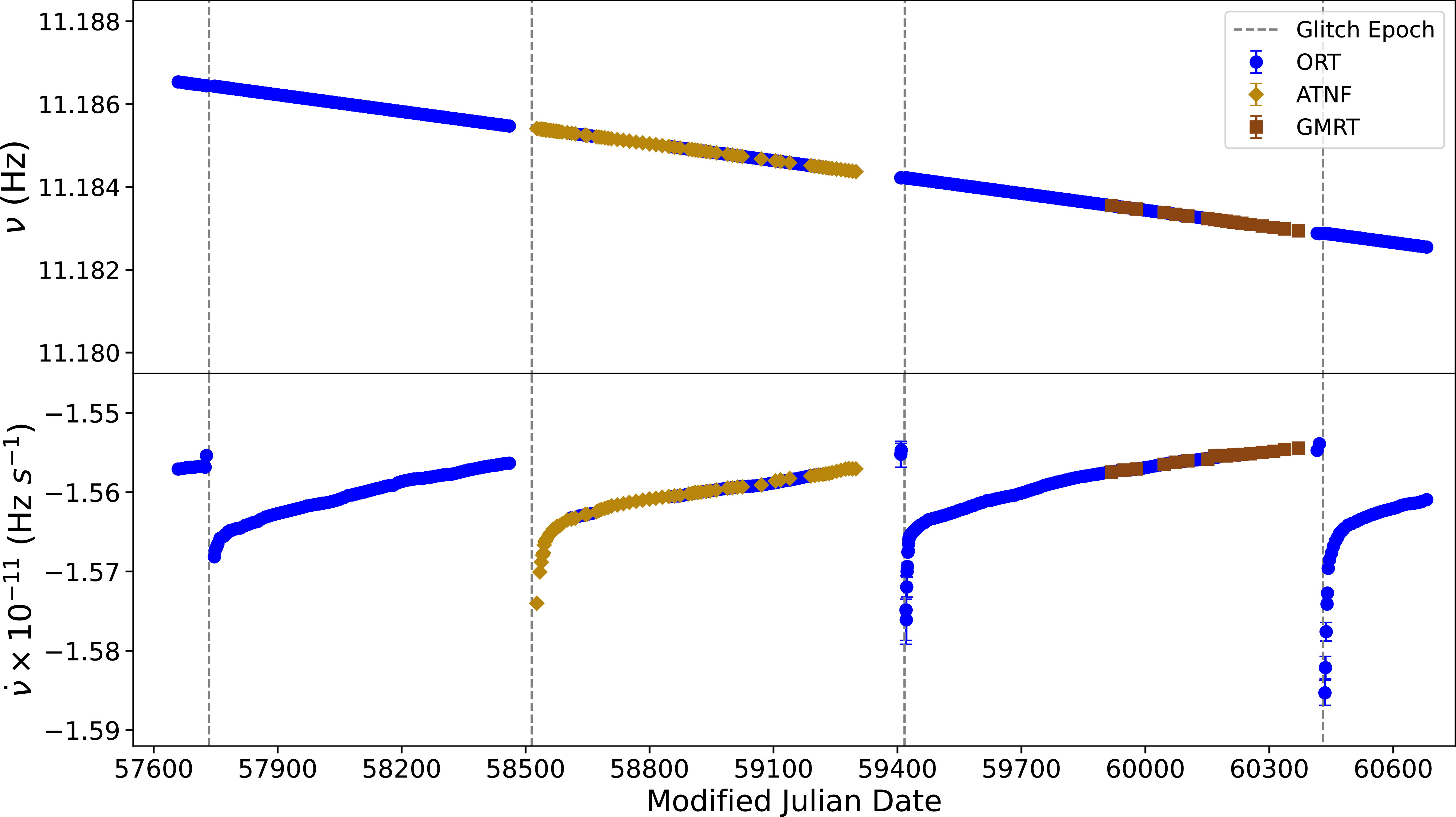
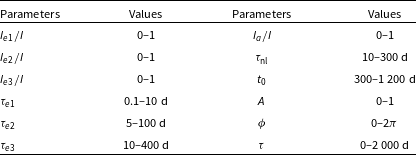


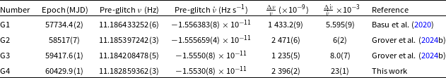
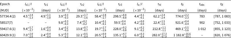
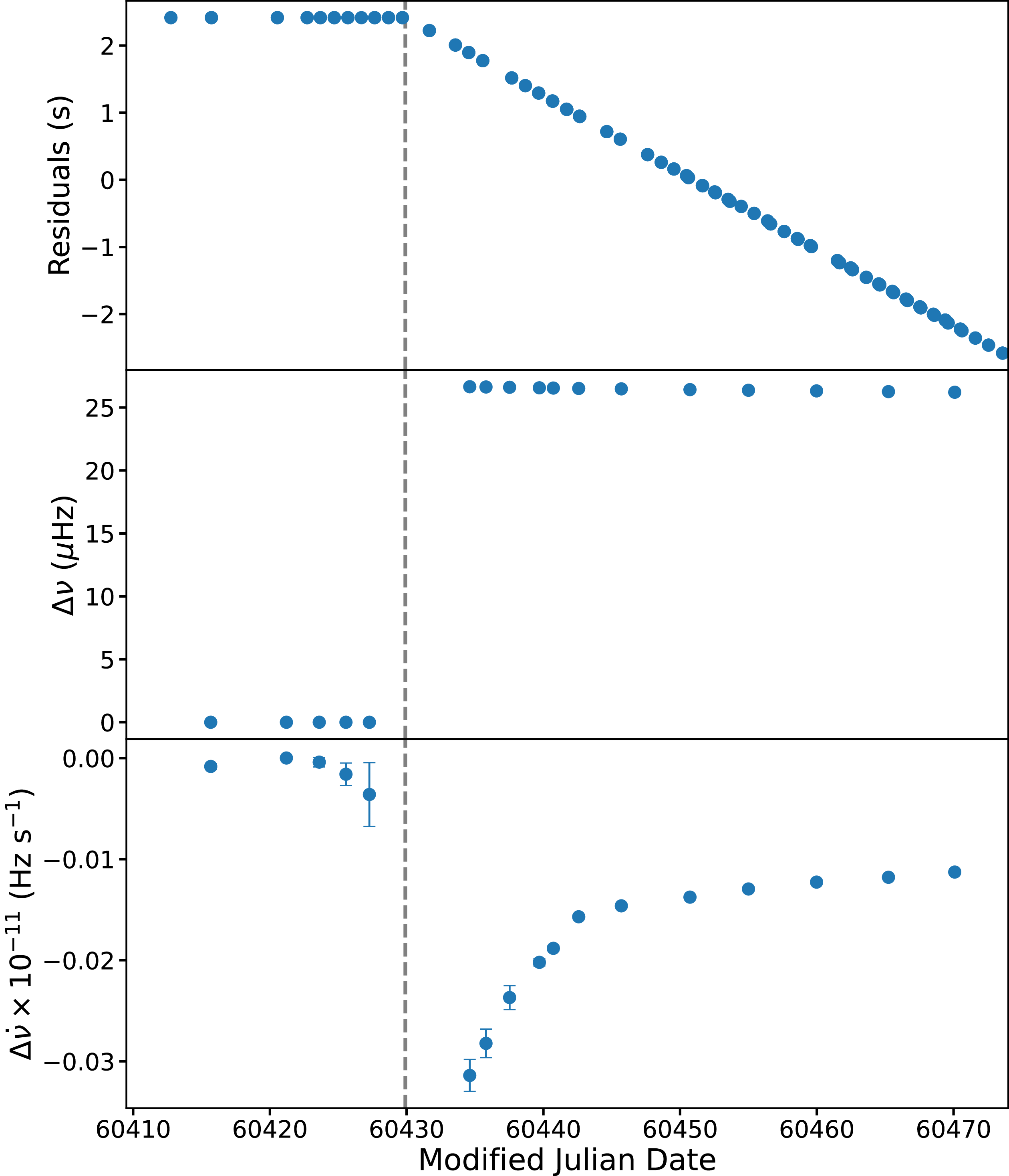


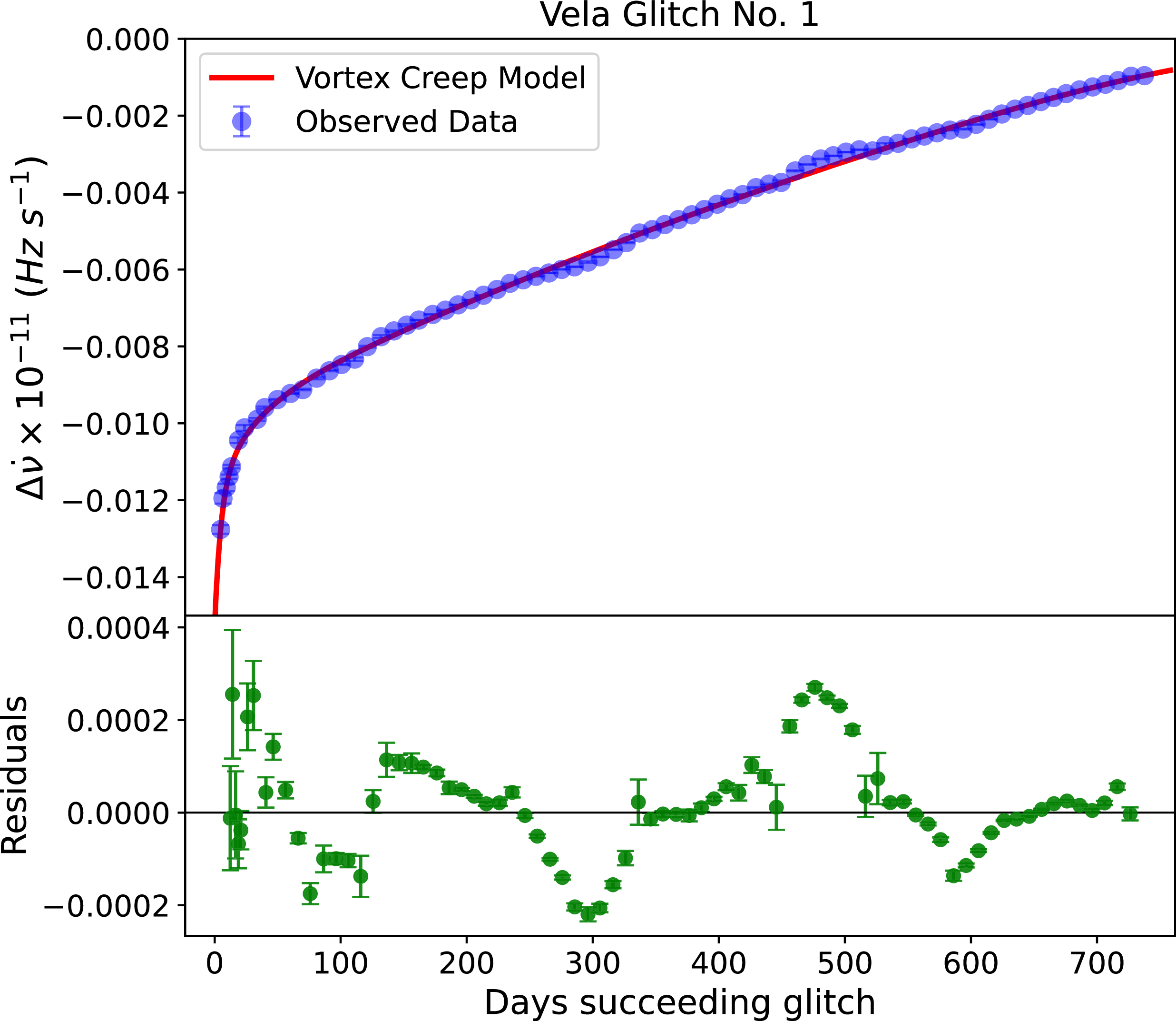


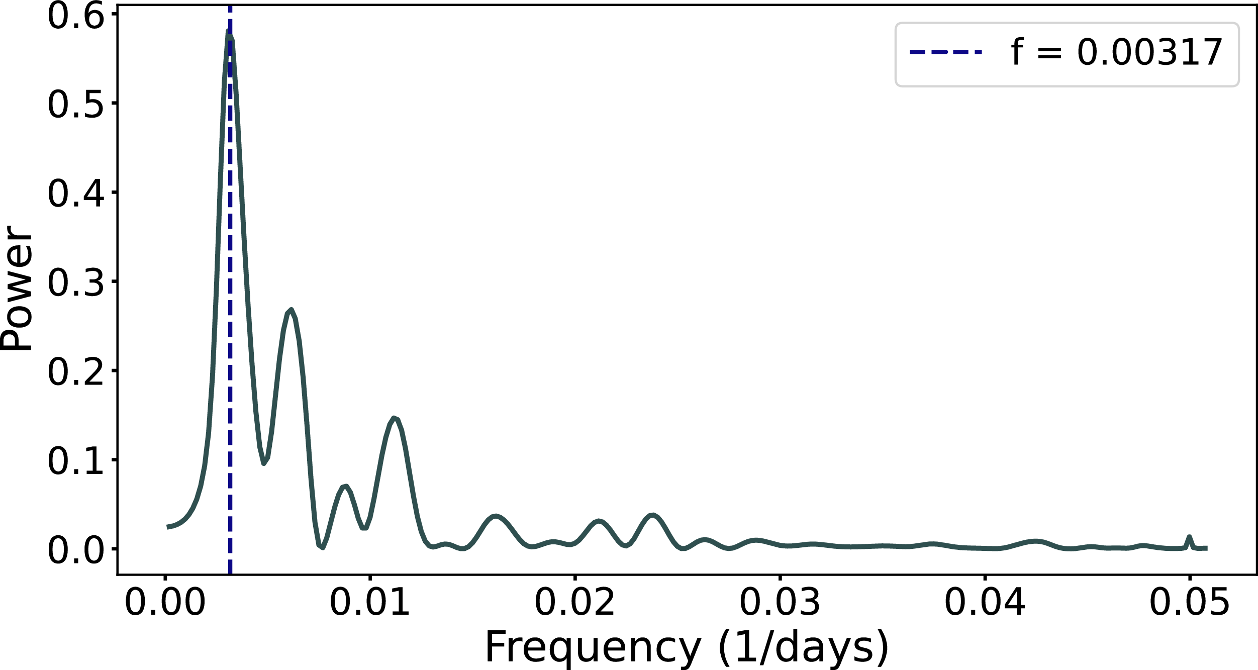
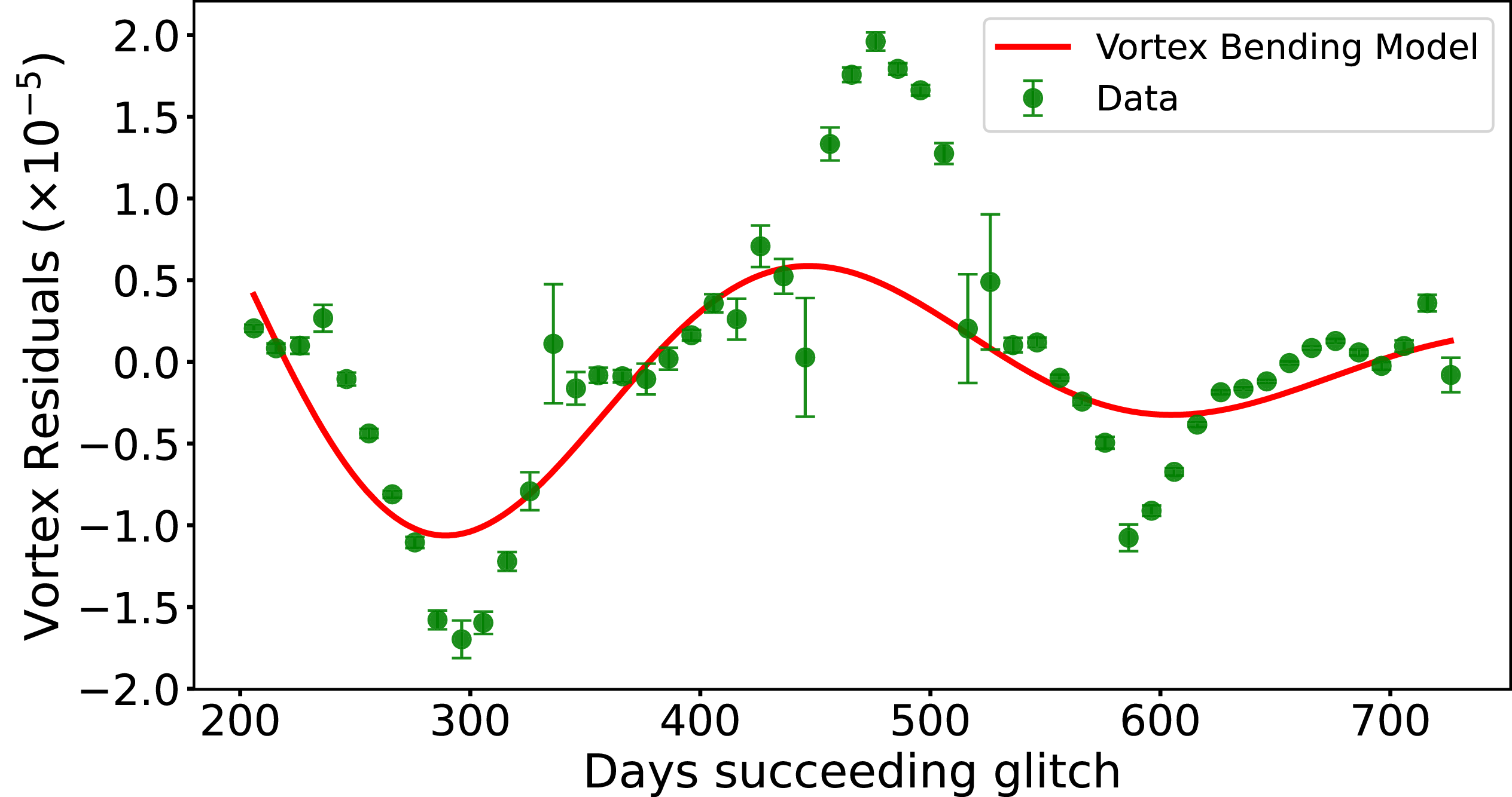


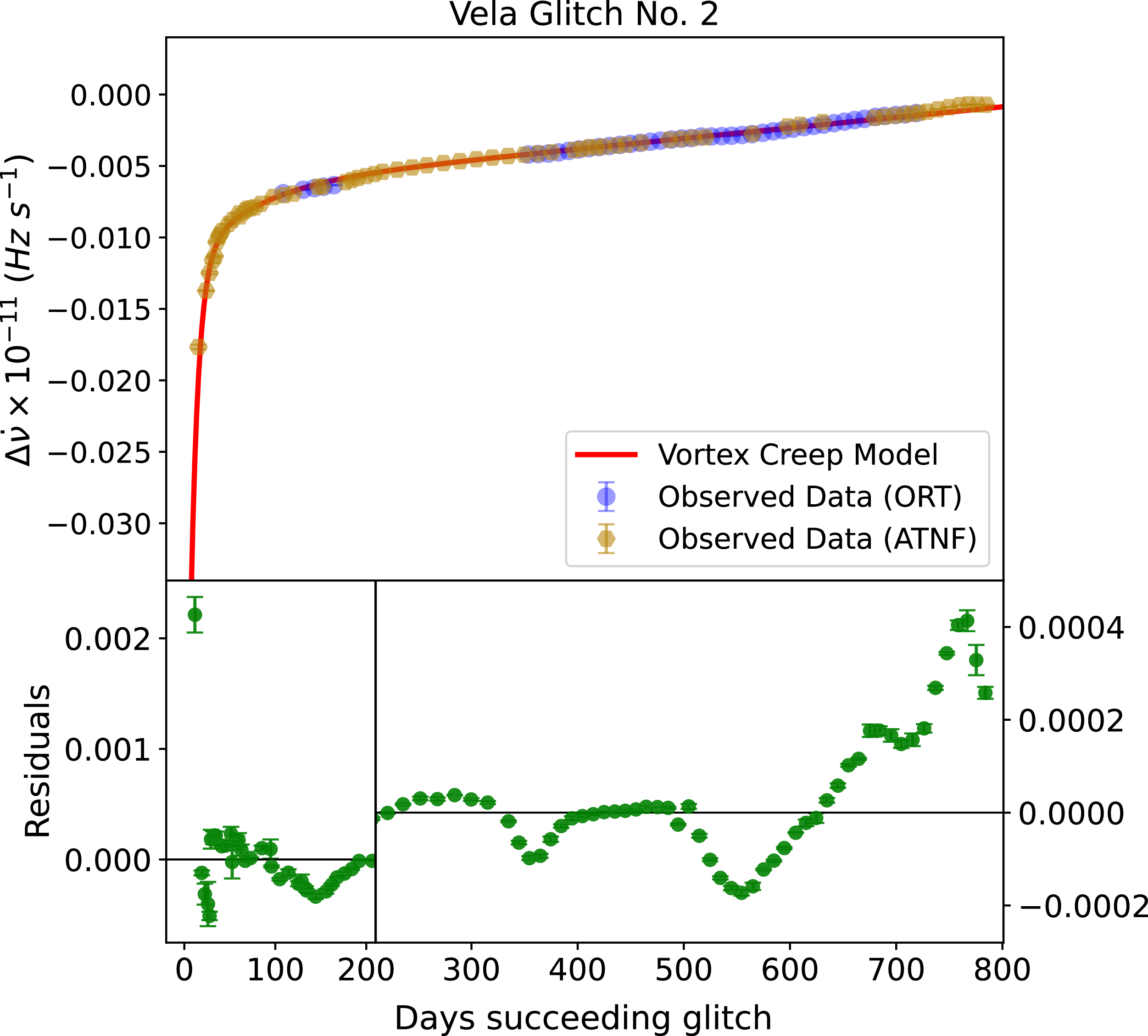


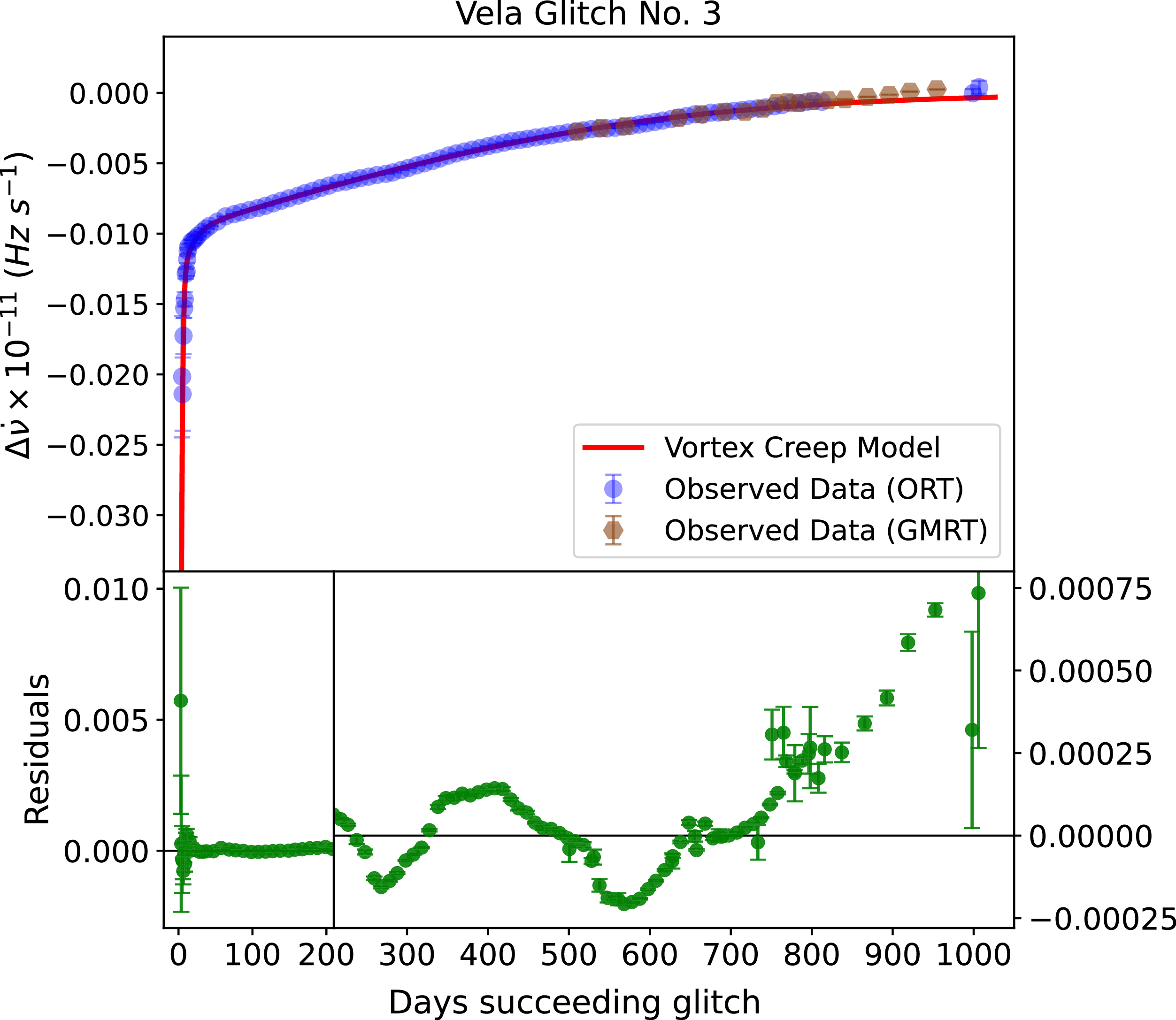
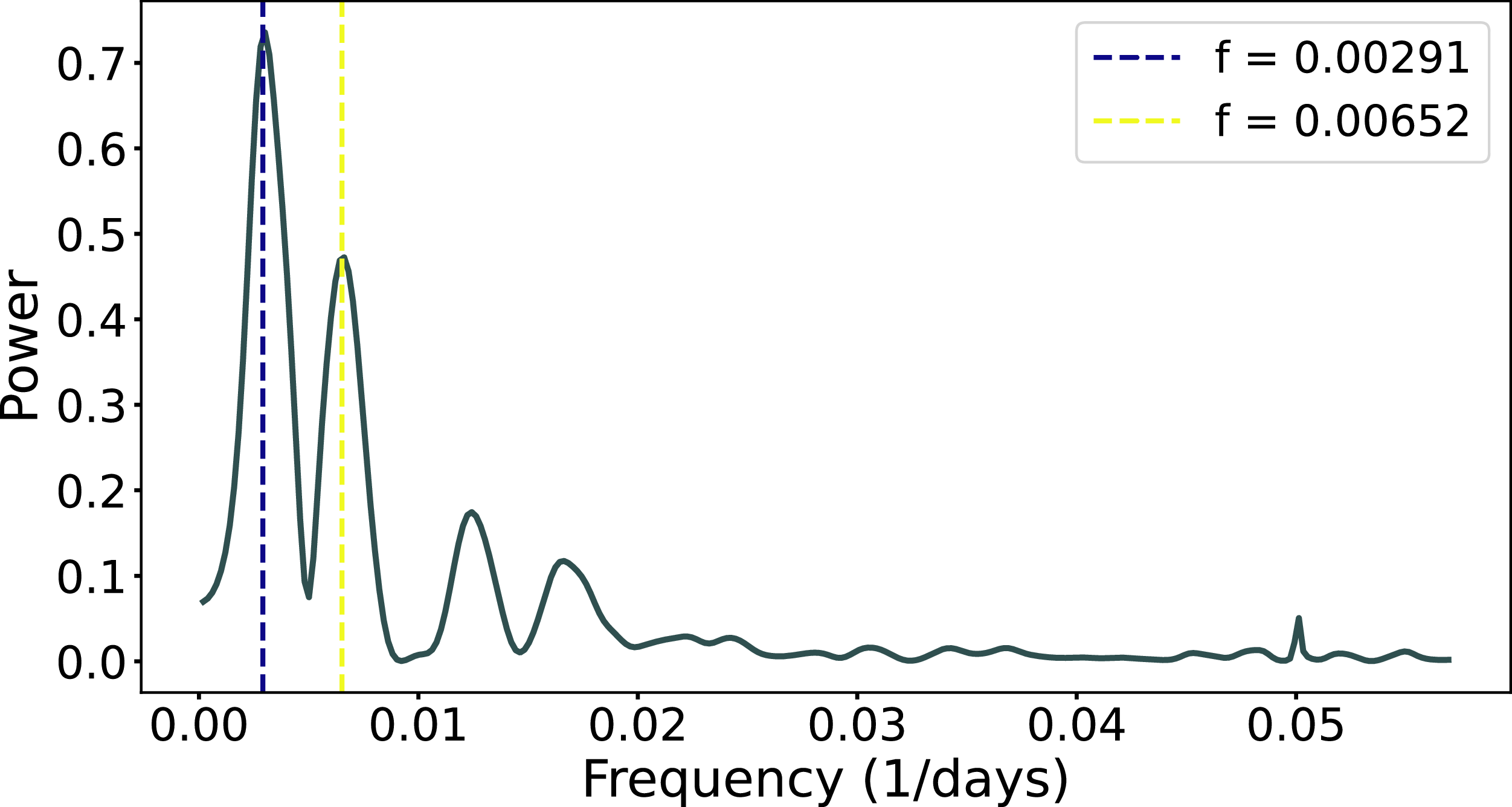
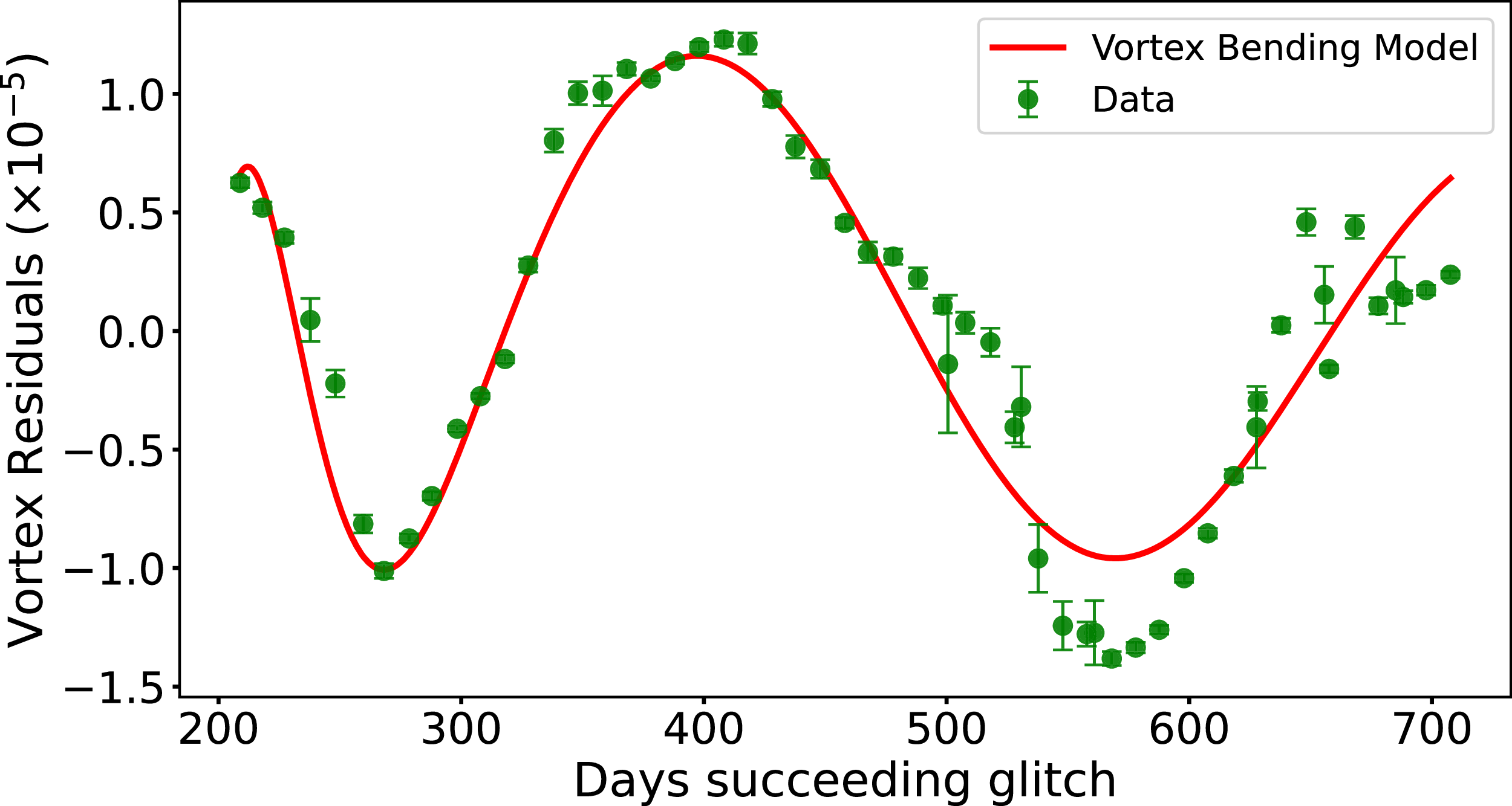


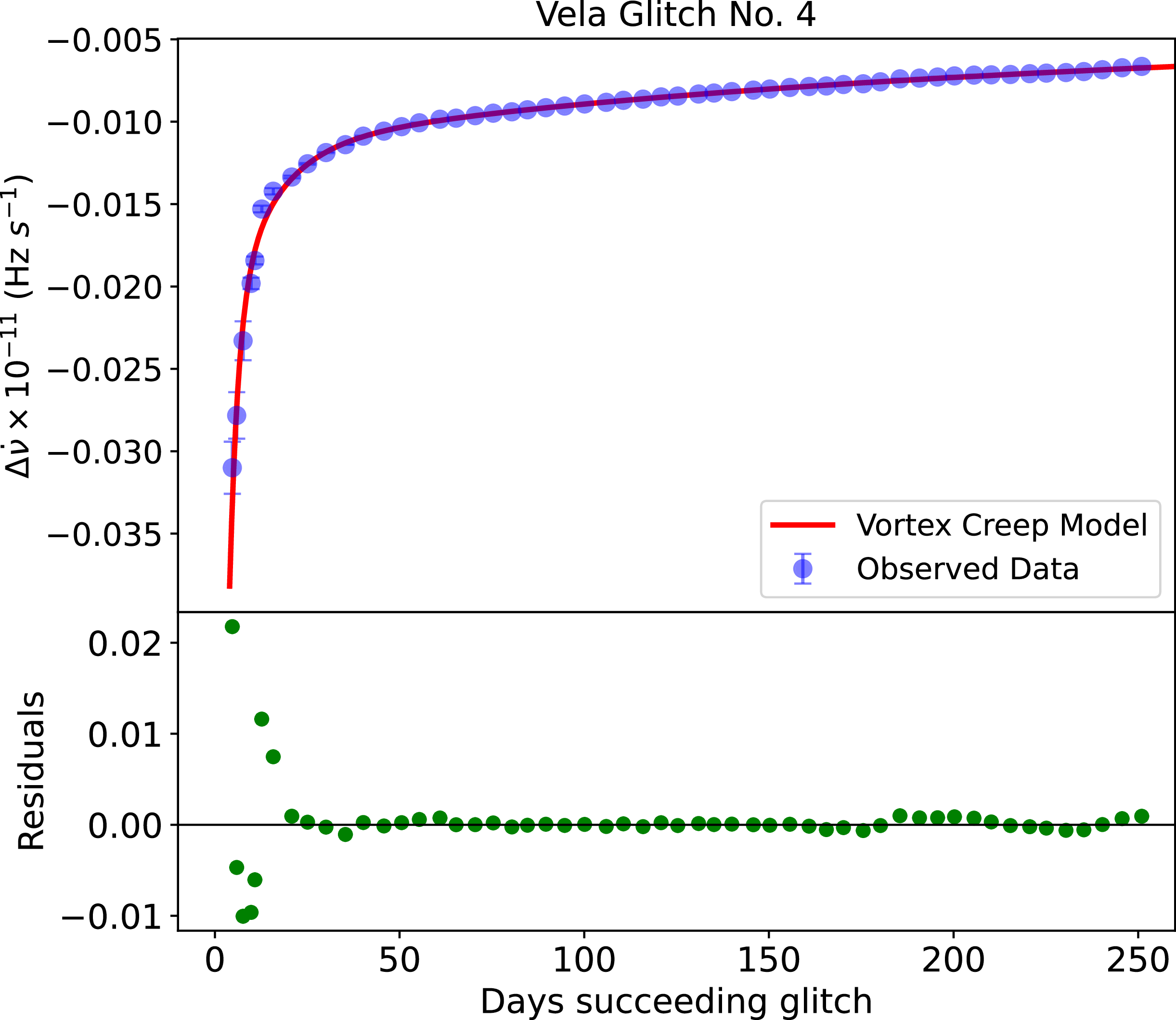
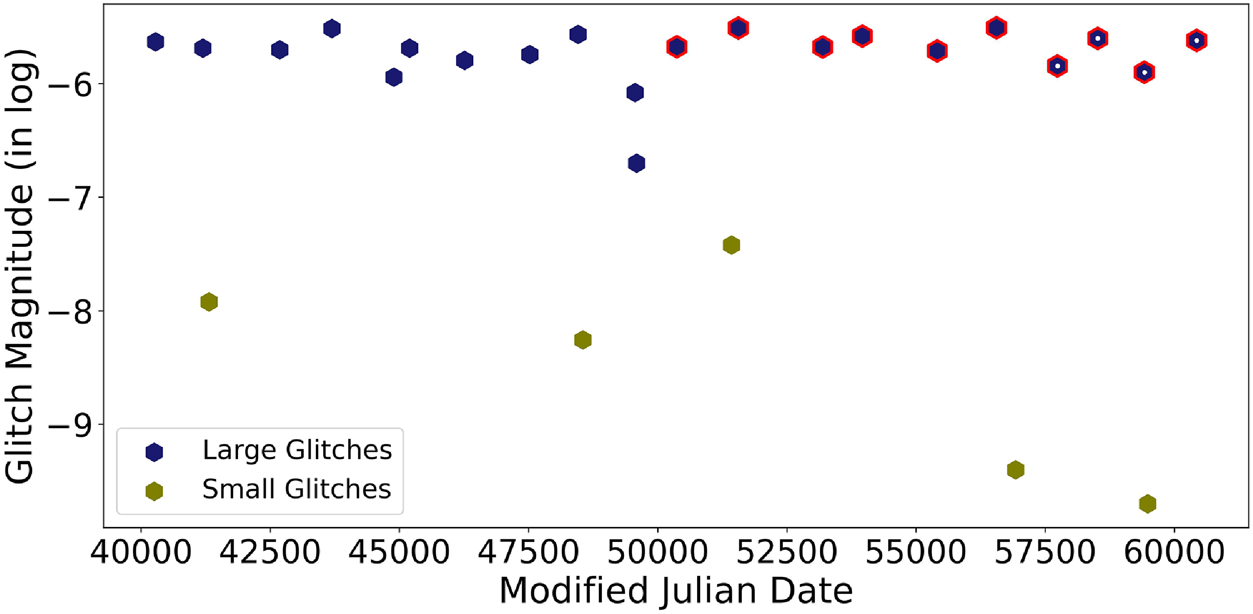
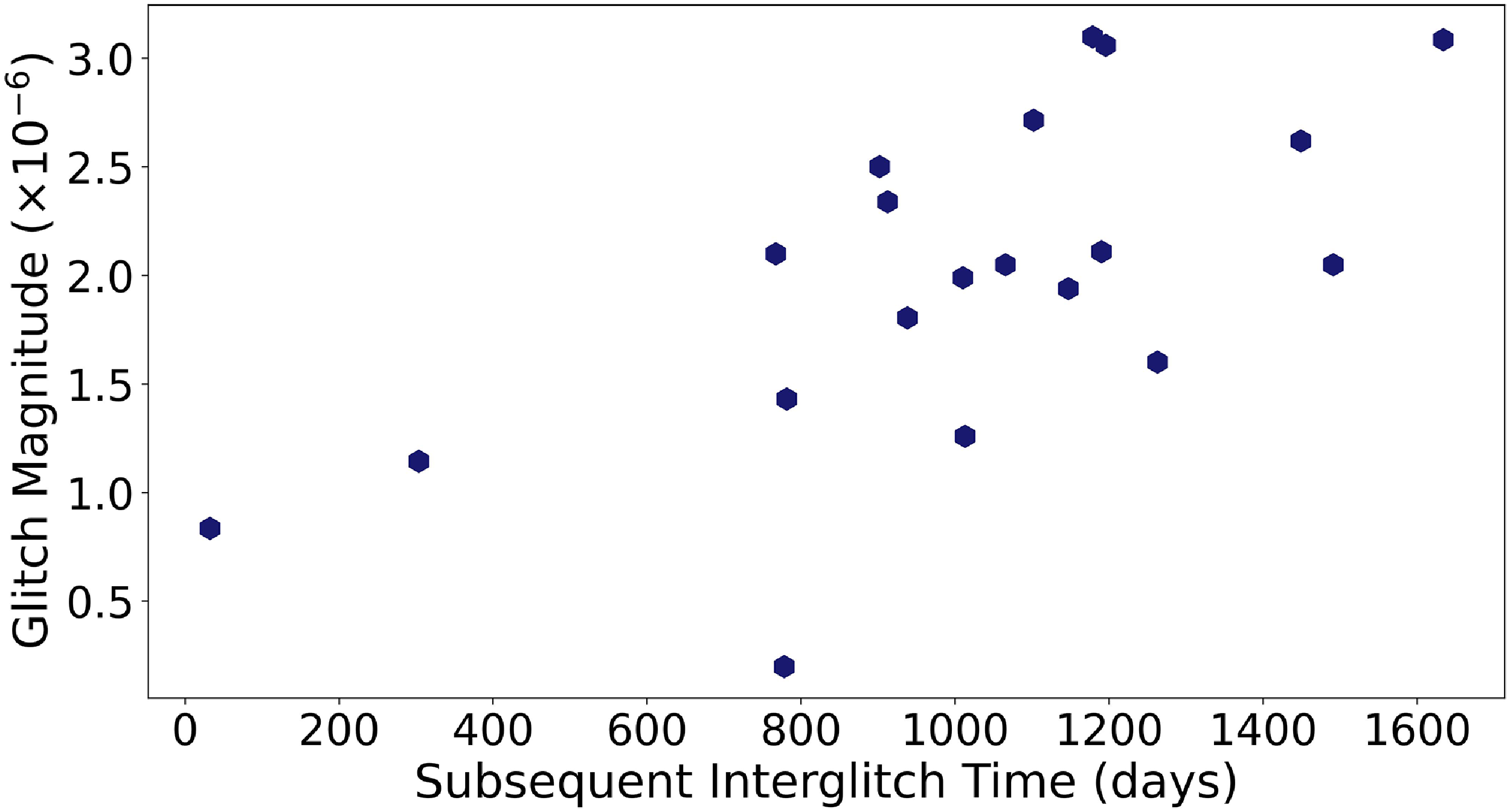

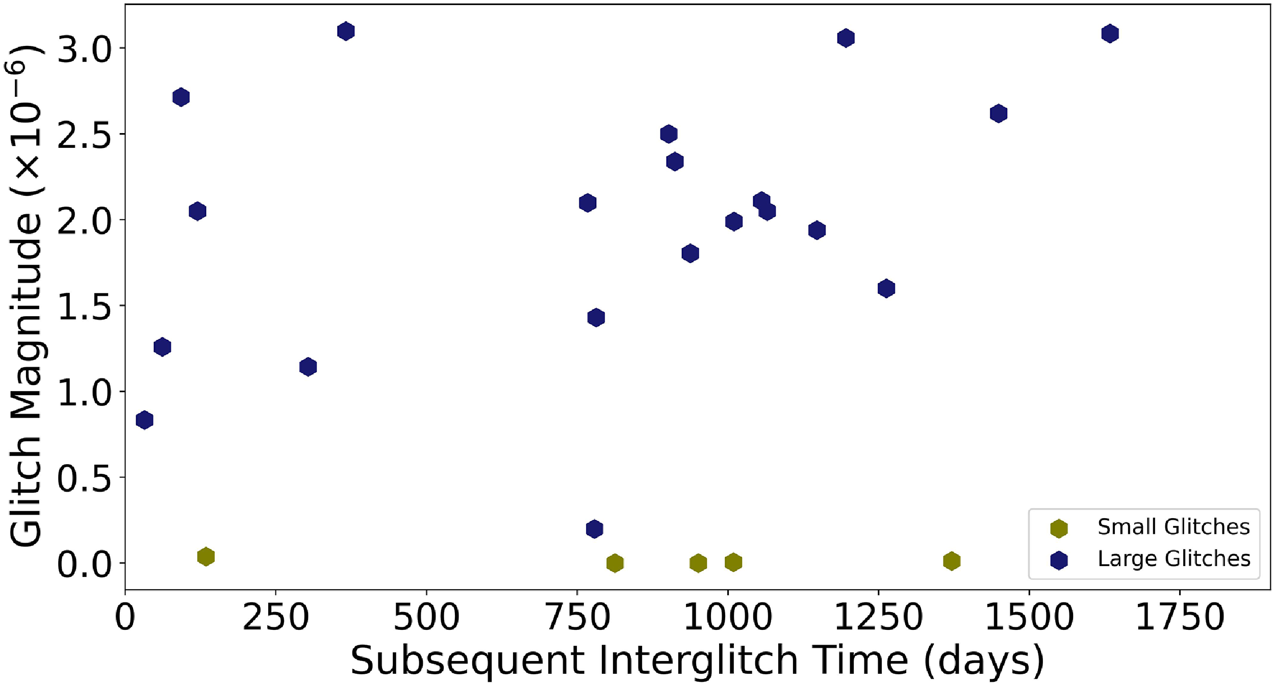
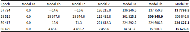

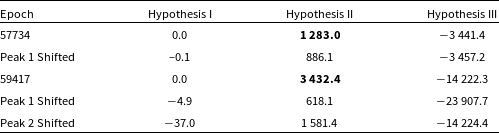

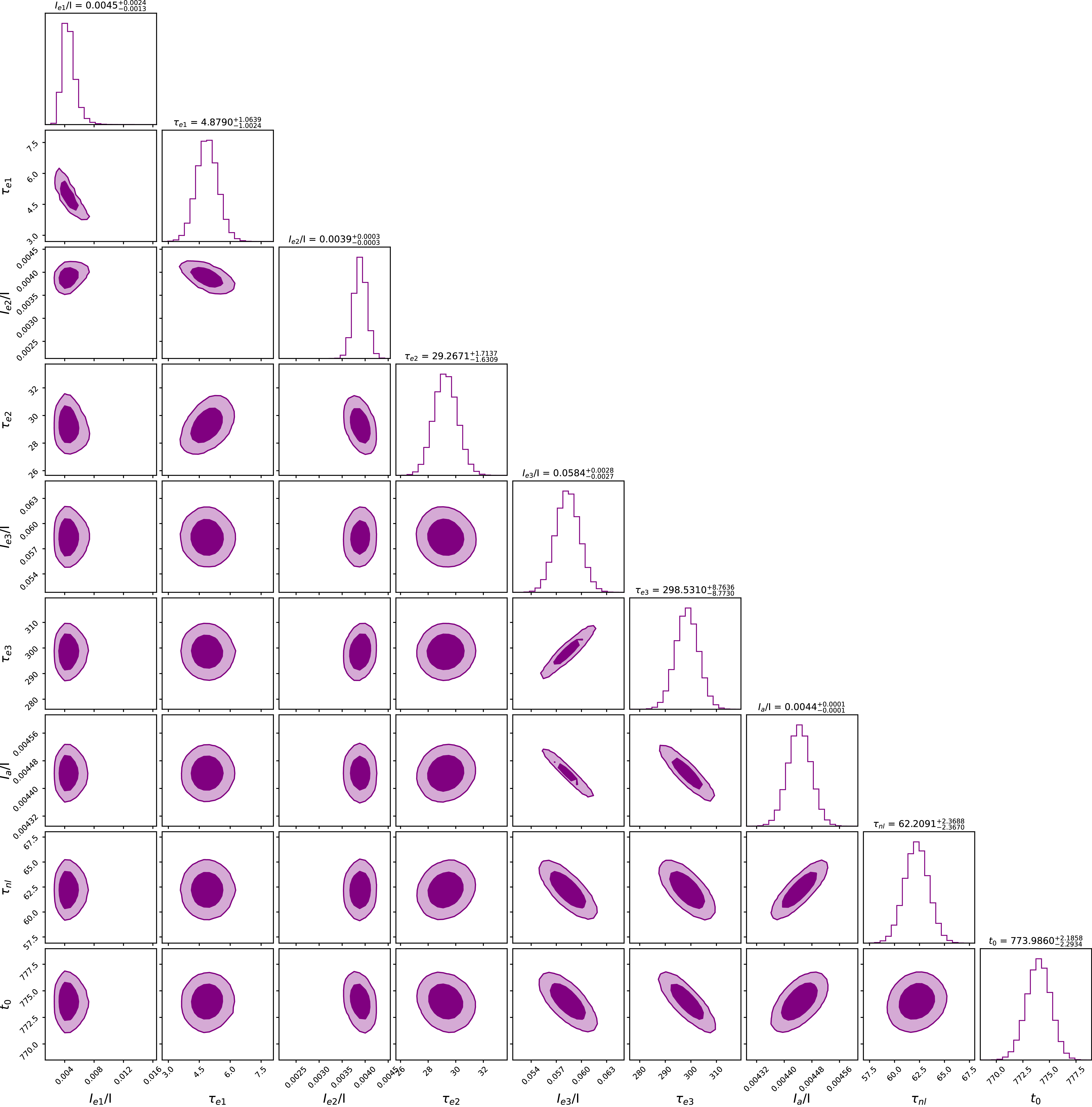


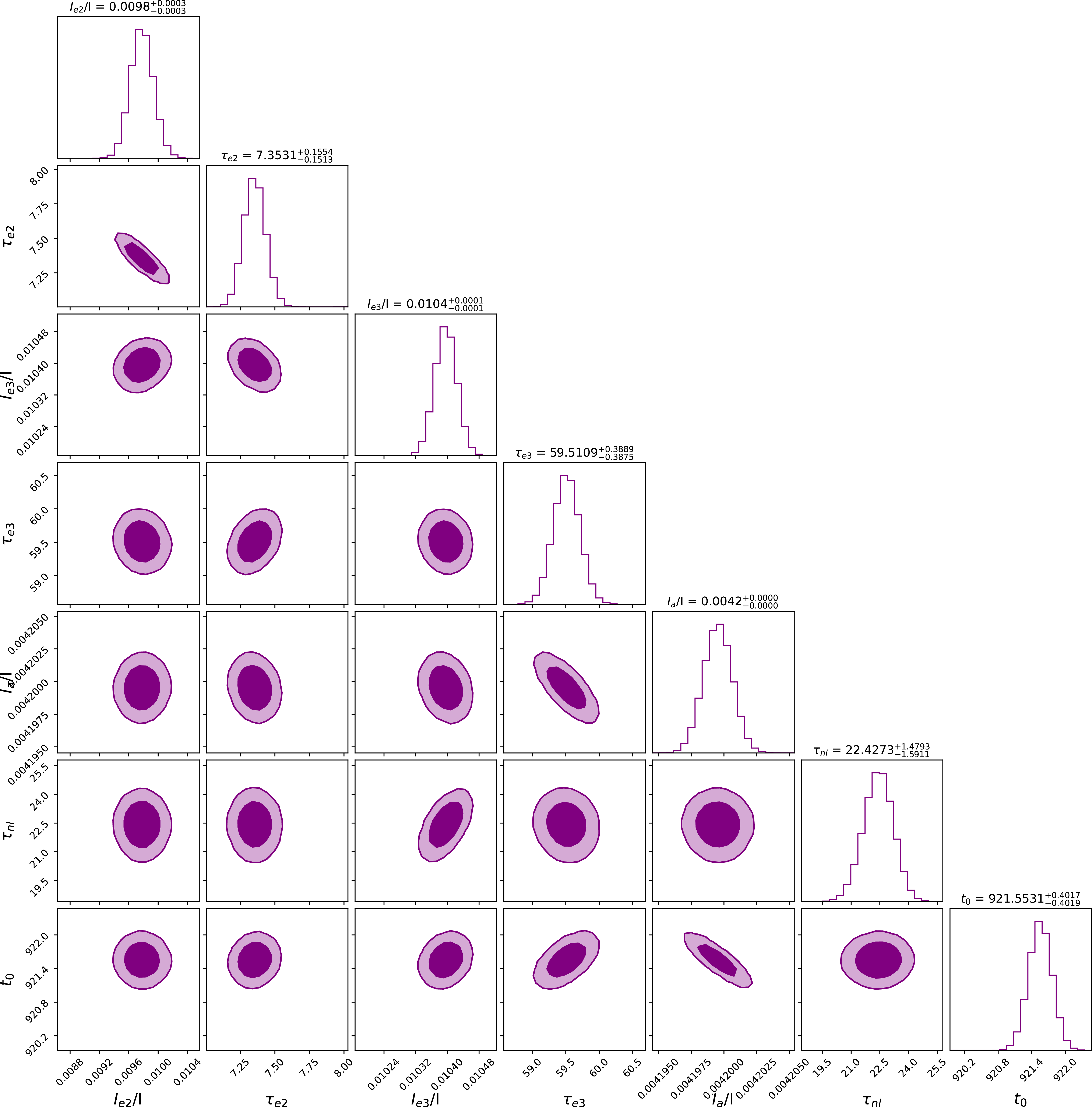


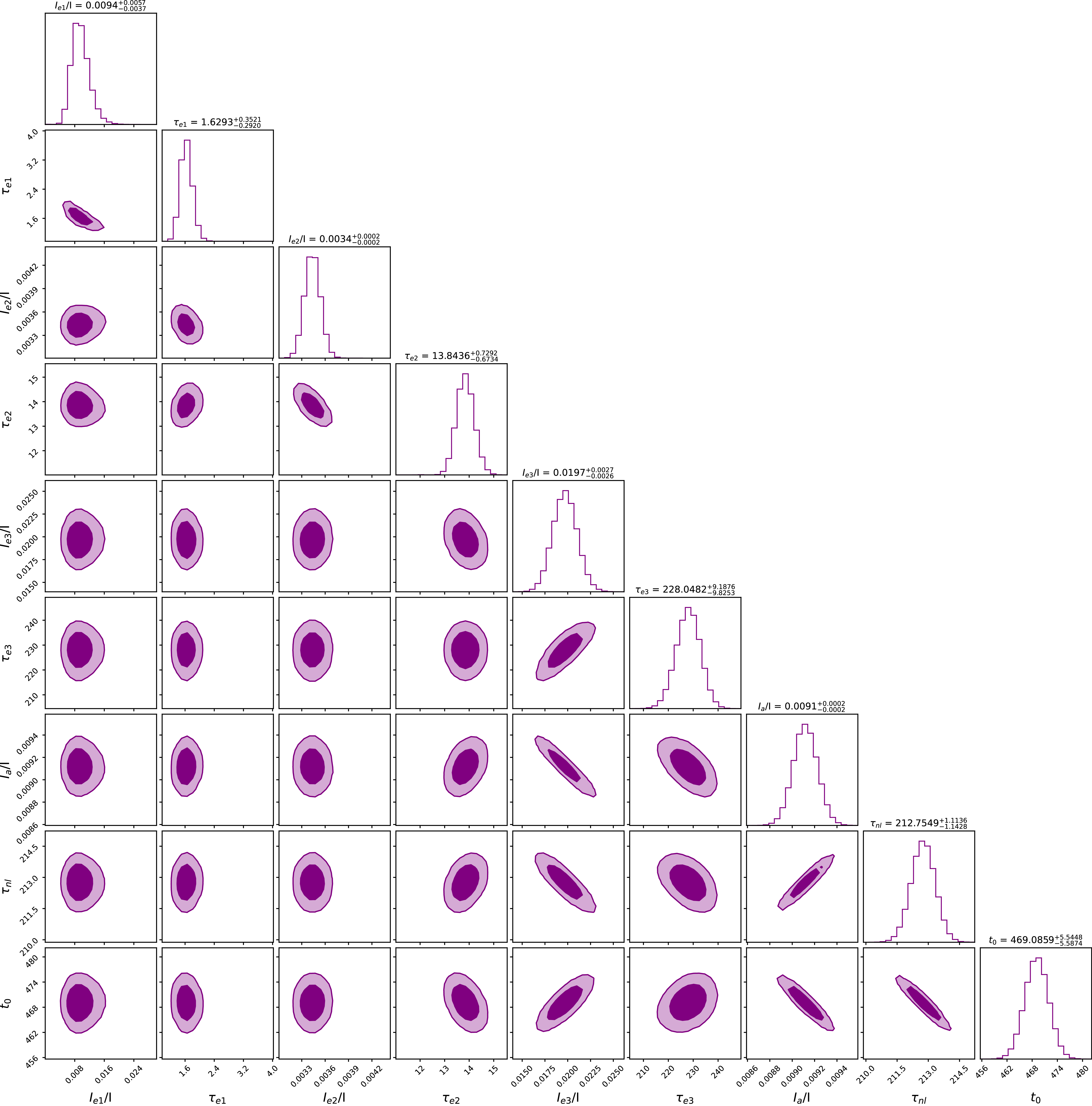


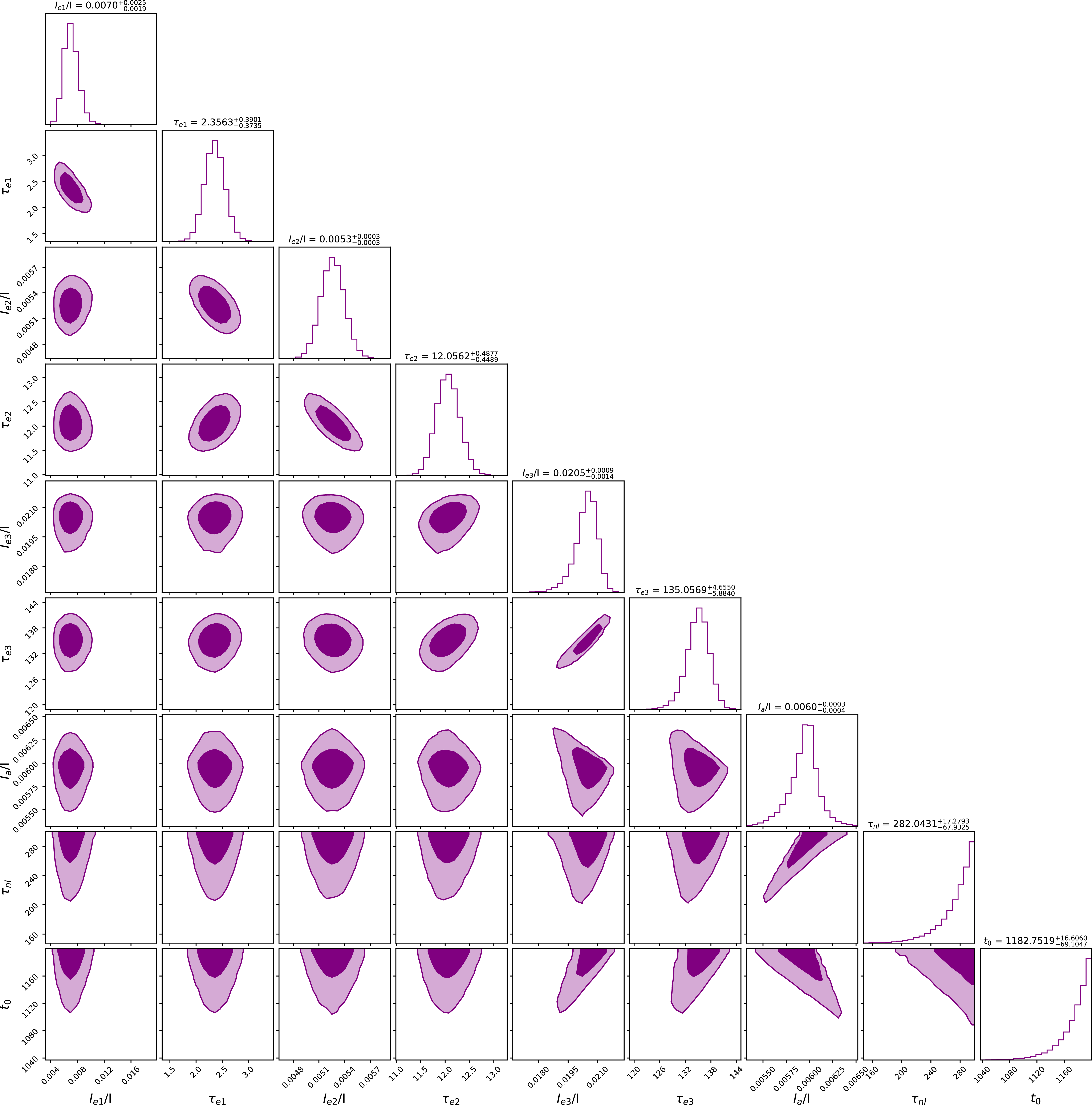


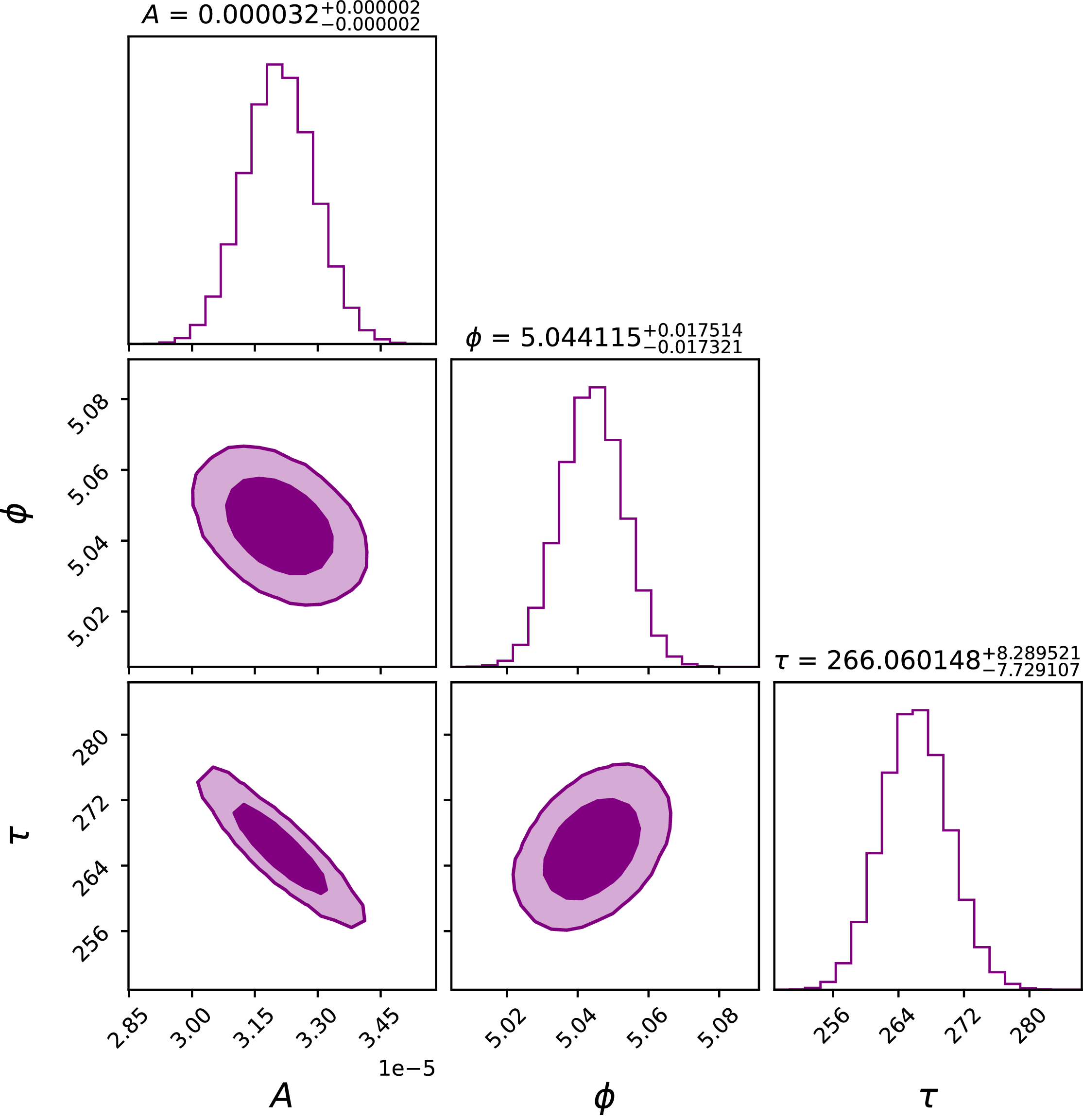


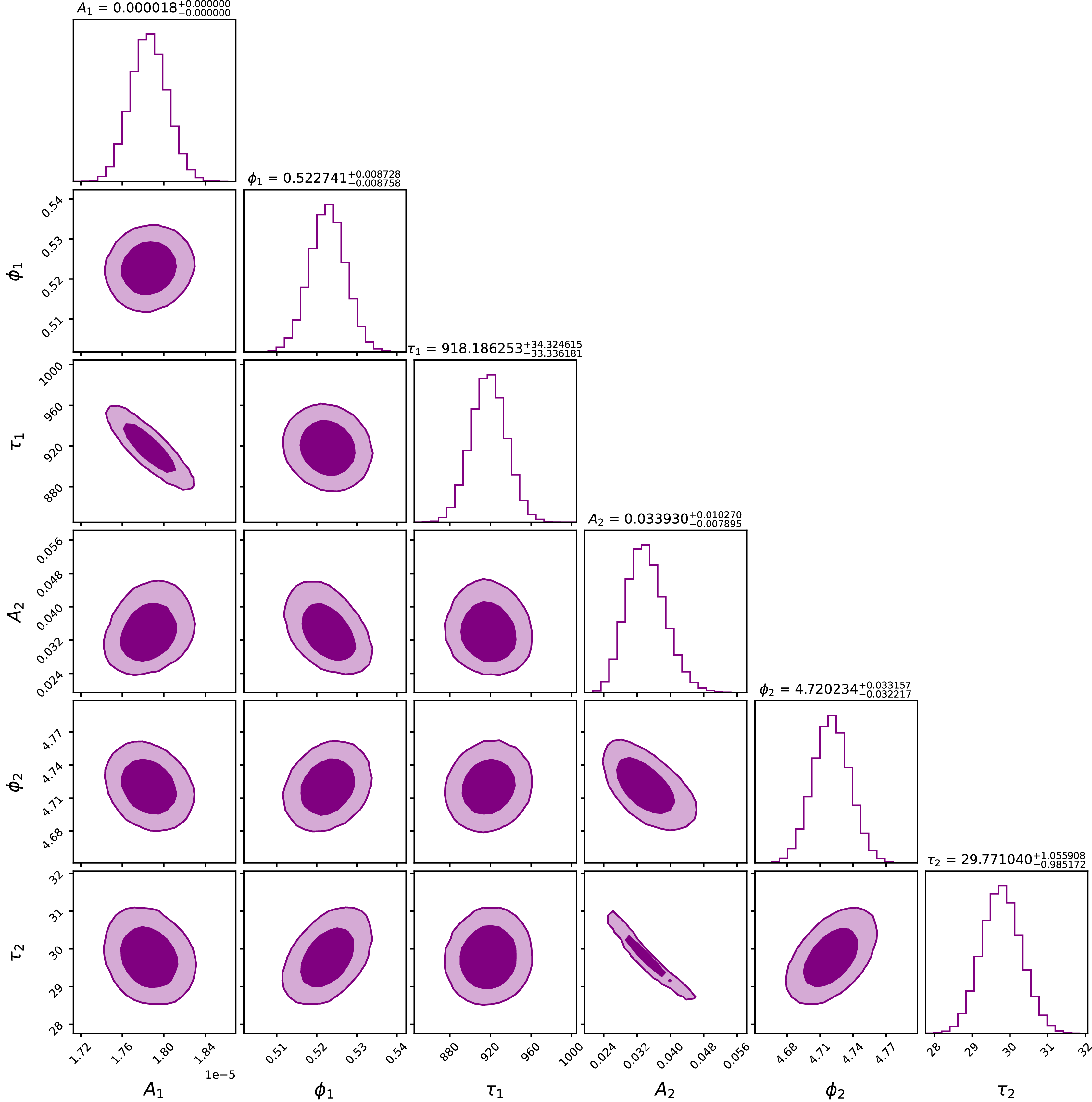


 Open access