





Impact Statement
Fan-array wind tunnels have the potential to produce arbitrary flow fields by simply adjusting the speeds of fans arranged in a grid. This potential is locked behind the complexity of the turbulent fluid dynamics. There does not exist a general process to find what combination of fan speeds best approximates a desired flow field in a fan array. In this work, we present a method to model the map from profiles of fixed fan speeds to profiles of time-averaged streamwise velocity. We also present a method for ‘inverse design’ that uses said model to estimate what profile of fan speeds will best produce a target velocity profile. We physically interpret our surrogate model, and experimentally validate both model predictions and inverse-design tracking. By resolving the case of static fan speeds to time-averaged streamwise velocities, this work serves as a foundational step towards fully resolved, generalised fan-array modelling and control.
1. Introduction
Fan-array wind tunnels (i.e. fan arrays, fan walls, multi-fan wind tunnels or real weather wind tunnels) provide an unprecedented ability to tailor fluid flows through the independent actuation of multiple fans. Compared with traditional wind tunnels with a single impeller, fan arrays have a smaller footprint for the same test-section size, have faster ramp times and produce slower, more turbulent flows (Dougherty, Reference Dougherty2022). The most salient feature of fan arrays is the independent actuation of each fan. Partitioning the flow source into independent units allows for spatial variation at the length scale of one fan diameter (Dougherty, Reference Dougherty2022), where the number of achievable flow profiles grows exponentially with the number of fans. Additionally, due to their small size and mass, each fan can change speed throughout an experiment, allowing for time-dependent flow variation.
The fan-array architecture has enabled novel wind-tunnel research across a wide range of applications. Veismann et al. (Reference Veismann, Dougherty, Rabinovitch, Quon and Gharib2021
a) used the space efficiency of fan arrays to conduct flight tests in a chamber replicating the Martian atmosphere for the Ingenuity Mars Helicopter. Dougherty (Reference Dougherty2022) used the independent actuation of 2,592 fans, arranged in a 3 $\times$
3 m grid, to produce compound shear layers and ‘checkerboard’ patterns in wind, then varied fan speeds sinusoidally to perturb shear-layer vortex-shedding frequencies, in an effort to replicate ‘flight-relevant environments’. O’Connell et al. (Reference O’Connell, Shi, Shi, Azizzadenesheli, Anandkumar, Yue and Chung2022) used the same fan array, modulated sinusoidally, to produce dynamic wind conditions to develop, train and test the deep-learning autonomous flight scheme Neural-Fly. More examples of research leveraging fan arrays range from studies on flies (Lopez, Reference Lopez2021) to atmospheric turbulence (Smith et al., Reference Smith, Masters, Liu and Reinhold2012; Ozono & Ikeda Reference Ozono and Ikeda2018; Cui et al., Reference Cui, Zhao, Cao and Ge2021; Veismann & Gharib, Reference Veismann and Gharib2019; Veismann & Gharib, Reference Veismann and Gharib2020; Yos et al., Reference Yos, Gharib and Veismann2019; Veismann et al., Reference Veismann, Wei, Conley, Young, Delaune, Burdick, Gharib and Izraelevitz2021
b; Dabiri et al., Reference Dabiri, Howland, Fu and Goldshmid2023; Mokhtar et al., Reference Mokhtar, Fernández-Cabán and Catarelli2023; Walpen et al., Reference Walpen, Catry and Noca2023; Wei & Dabiri, Reference Wei and Dabiri2022); to autonomous flight on Earth (Olejnik et al., Reference Olejnik, Wang, Dupeyroux, Stroobants, Karasek, De and de2022; Renn, Reference Renn2023; Wang et al., Reference Wang, Kjellberg, Catry, Bosson, Sanyal and Glauser2021); and on Mars (Veismann, Reference Veismann2022).
$\times$
3 m grid, to produce compound shear layers and ‘checkerboard’ patterns in wind, then varied fan speeds sinusoidally to perturb shear-layer vortex-shedding frequencies, in an effort to replicate ‘flight-relevant environments’. O’Connell et al. (Reference O’Connell, Shi, Shi, Azizzadenesheli, Anandkumar, Yue and Chung2022) used the same fan array, modulated sinusoidally, to produce dynamic wind conditions to develop, train and test the deep-learning autonomous flight scheme Neural-Fly. More examples of research leveraging fan arrays range from studies on flies (Lopez, Reference Lopez2021) to atmospheric turbulence (Smith et al., Reference Smith, Masters, Liu and Reinhold2012; Ozono & Ikeda Reference Ozono and Ikeda2018; Cui et al., Reference Cui, Zhao, Cao and Ge2021; Veismann & Gharib, Reference Veismann and Gharib2019; Veismann & Gharib, Reference Veismann and Gharib2020; Yos et al., Reference Yos, Gharib and Veismann2019; Veismann et al., Reference Veismann, Wei, Conley, Young, Delaune, Burdick, Gharib and Izraelevitz2021
b; Dabiri et al., Reference Dabiri, Howland, Fu and Goldshmid2023; Mokhtar et al., Reference Mokhtar, Fernández-Cabán and Catarelli2023; Walpen et al., Reference Walpen, Catry and Noca2023; Wei & Dabiri, Reference Wei and Dabiri2022); to autonomous flight on Earth (Olejnik et al., Reference Olejnik, Wang, Dupeyroux, Stroobants, Karasek, De and de2022; Renn, Reference Renn2023; Wang et al., Reference Wang, Kjellberg, Catry, Bosson, Sanyal and Glauser2021); and on Mars (Veismann, Reference Veismann2022).
The breadth of successful applications of fan arrays has motivated work on their flow characterisation, physics modelling and flow prescription in recent years. Veismann et al. (Reference Veismann, Dougherty, Rabinovitch, Quon and Gharib2021
a) determined a fan array’s functional test section (the sub-volume where boundary effects are minimal) when using a flush-mounted honeycomb for flow conditioning. Di Luca et al. (Reference Di, Matteo and Noca2024
a) designed multi-layered flow management devices to improve fan-array flow quality, reducing turbulence intensity to a level seen in traditional, single-impeller wind tunnels (from $7\,\%$
to
$7\,\%$
to $0.45\,\%$
) at the cost of reduced momentum output. Dougherty (Reference Dougherty2022) showed that dual- and triple-stream free shear layers generated by fan arrays follow the same self-similarity and scaling laws as traditional ‘splitter plate’ shear layers (Brown & Roshko, Reference Brown and Roshko1974). Dougherty (Reference Dougherty2022) also derived an analytical model for the free-stream velocity of an array with all fans set to the same time-varying speed. Di Luca et al. (Reference Di, Matteo and Noca2024
b) derived an analytical model for the streamwise velocity of multi-plane, compound shear flows with augmented flow conditioning. They found that this case is governed by the velocity ratio between adjacent fans, consistent with Dougherty (Reference Dougherty2022), and that their model generalises across downstream distances when normalised by fan width. Walpen et al. (Reference Walpen, Govoni, Stirnemann, Ionescu, Bosson, Catry and Noca2024) used a proportional control scheme to prescribe flow conditions enabled by feedback from a motion-tracked velocimetry system. This scheme was validated by tracking a uniform flow target of 8 m s−1 with mean absolute errors between 0.2 and 1 m s−1. Note how, across published works, fan width and total fan-array width appear as length scales of fan-array flows.
$0.45\,\%$
) at the cost of reduced momentum output. Dougherty (Reference Dougherty2022) showed that dual- and triple-stream free shear layers generated by fan arrays follow the same self-similarity and scaling laws as traditional ‘splitter plate’ shear layers (Brown & Roshko, Reference Brown and Roshko1974). Dougherty (Reference Dougherty2022) also derived an analytical model for the free-stream velocity of an array with all fans set to the same time-varying speed. Di Luca et al. (Reference Di, Matteo and Noca2024
b) derived an analytical model for the streamwise velocity of multi-plane, compound shear flows with augmented flow conditioning. They found that this case is governed by the velocity ratio between adjacent fans, consistent with Dougherty (Reference Dougherty2022), and that their model generalises across downstream distances when normalised by fan width. Walpen et al. (Reference Walpen, Govoni, Stirnemann, Ionescu, Bosson, Catry and Noca2024) used a proportional control scheme to prescribe flow conditions enabled by feedback from a motion-tracked velocimetry system. This scheme was validated by tracking a uniform flow target of 8 m s−1 with mean absolute errors between 0.2 and 1 m s−1. Note how, across published works, fan width and total fan-array width appear as length scales of fan-array flows.
The aforementioned studies are highlights of an actively growing body of work, each incrementally resolving fan-array physics and control. However, due to the large fan-array state space and the complexity of unsteady flow physics, designing arbitrary flows of the full available dimensionality remains an open challenge and, thus, the full capability of fan-array wind tunnels remains unavailable.
(a) Shows: (i) a fan-array wind tunnel (ii) is given static profiles of fan speeds that vary along one spanwise axis, $y$
. (iii) Mean profiles of streamwise velocity are measured by (iv) a sensor array along said axis,
$y$
. (iii) Mean profiles of streamwise velocity are measured by (iv) a sensor array along said axis, $y$
. (b) A vector of fan speeds
$y$
. (b) A vector of fan speeds $\boldsymbol{r}$
multiplied by a coefficient matrix
$\boldsymbol{r}$
multiplied by a coefficient matrix $\boldsymbol{A}$
plus a bias vector
$\boldsymbol{A}$
plus a bias vector $\boldsymbol{b}$
gives a predicted velocity profile
$\boldsymbol{b}$
gives a predicted velocity profile $\boldsymbol{v}_{\mathrm{pred}}$
.
$\boldsymbol{v}_{\mathrm{pred}}$
.

Prescribing flows in a fan array comes down to finding the right fan speeds, which can be done through inverse-design based on a surrogate model. A surrogate model predicts the behaviour of the fan array (given fan speeds, what flow is produced), and can be used to answer the inverse question: Given a target flow, what fan speeds produce it? This process is often referred to as ‘inverse design’, and has been applied successfully in systems with a complex fluid dynamics. For example, Du et al. (Reference Du, He and Martins2021), Sekar et al. (Reference Sekar, Zhang, Shu and Khoo2019) and Gardner & Selig (Reference Gardner and Selig2012) used data-driven modelling for inverse design of airfoil shapes. An inverse-design scheme, once validated, can be used entirely without sensor feedback, freeing the fan-array test section; or it can be used within a feedback loop to converge in less time with fewer sensors of lower resolution. A surrogate model that spans the full space of achievable temporally and spatially varying flows is infeasible to resolve in a single study, but it can be partitioned and systematically modelled in stages.
In this work, we focus on the case of time-averaged streamwise velocity profiles produced by steady fan speeds. We couple one axis of our fan array such that all rows of fans have the same speed and only one spanwise axis is non-homogenous (so our flow profiles are ‘one-dimensional’, as shown in figure 1 a). We produce, validate and interpret a surrogate model and an inverse-design scheme for this special case.
We find that a regularised linear map is an effective surrogate model for these ‘one-dimensional, static’ fan-array instances. Linear methods are often chosen in fields such as fluid dynamics for their simplicity and interpretability (Manohar et al. (Reference Manohar, Brunton, Kutz and Brunton2018), which is the case in this work. Our linear map, encoded as a coefficient matrix and a bias vector, shown in figure 1(b), is both parsimonious and interpretable. Our resulting model coefficients match intuition: each velocity reading is primarily affected by the fan row directly upstream of it, is secondarily affected by adjacent fan rows and is insensitive to distant fan rows. Fitting models on profiles measured further away from the source appears to capture the effect of turbulent mixing and entrainment, visible as a ‘smearing’ of model coefficients (shown in figure 4). The streamwise evolution of model coefficients is found to be self-similar under the canonical similarity transform of a time-averaged round jet, suggesting our surrogate model converged to a solution of superimposed round-jet profiles centred on each fan in the array (Section 3.1.1).
We apply this model for inverse design as the basis of a quadratic program to find the best fan speeds for desired velocity profiles, in a manner comparable to how linear models are used in model-predictive control (Muske & Rawlings, Reference Muske and Rawlings1993). Our quadratic program supports constraints on fan speeds, which are critical in practice, where noise restrictions, power limitations and fan-unit failure will impose requirements on fan-array control that cannot be accounted for at the time of model fitting. We experimentally validate both out-of-sample prediction and open-loop tracking performance using inputs and targets produced after fitting. This work presents, to our knowledge, the first data-driven surrogate model of fan-array wind-tunnel flow profiles, together with the first demonstration of model-based constrained optimal flow control on fan-array flow.
This paper is structured as follows: in Section 2 we describe our fan array (Section 2.1.1), sensors (Section 2.1.2), mathematics (Section 2.2) and dataset (Section 2.3); in Section 3 we present the resulting model coefficients (Section 3.1) and their physical interpretation (Section 3.1.1), as well as the prediction (Section 3.2) and tracking performance (Section 3.3) measured in validation experiments; Section 4 contains concluding remarks and considerations for future research towards fully resolved, generalised fan-array modelling and control.
2. Methods
2.1. Experimental design
2.1.1. Fan-array wind tunnel
The model and control method presented in this paper are built entirely on experimentally collected fan-array data. There are three signals in a fan-array flow experiment: (i) the control signal to each fan, (ii) the speed (rotational rate) of each fan and (iii) the flow measured at some downstream location. Fan control signals are encoded as pulse-width modulation duty cycle, which ranges from $0$
or
$0$
or $0\,\%$
(lowest fan speed, 1550 RPM) to
$0\,\%$
(lowest fan speed, 1550 RPM) to $1$
or
$1$
or $100\,\%$
(highest fan speed, 5500 RPM). Fan speed is measured in revolutions per minute (RPM). Average RPM versus duty cycle for all fans is shown in figure 2(c). Flow is measured in its streamwise component (
$100\,\%$
(highest fan speed, 5500 RPM). Fan speed is measured in revolutions per minute (RPM). Average RPM versus duty cycle for all fans is shown in figure 2(c). Flow is measured in its streamwise component ( $x$
) only, is averaged in time and is normalised by
$x$
) only, is averaged in time and is normalised by $V_{\mathrm{max}}=11\ \mathrm{m\,s}^{-1}$
, which is the maximum wind speed of this fan array. The minimum wind speed is
$V_{\mathrm{max}}=11\ \mathrm{m\,s}^{-1}$
, which is the maximum wind speed of this fan array. The minimum wind speed is $2\ \mathrm{m\,s}^{-1}$
. We use a
$2\ \mathrm{m\,s}^{-1}$
. We use a $10\times 10$
array of DELTA PFC1212DE-F00
$10\times 10$
array of DELTA PFC1212DE-F00 $120\times 120\,\mathrm{mm}$
fan units. This array spans a square
$120\times 120\,\mathrm{mm}$
fan units. This array spans a square $1.22\times 1.22\,\mathrm{m}$
(spanwise) enclosed open-loop test section that extends
$1.22\times 1.22\,\mathrm{m}$
(spanwise) enclosed open-loop test section that extends $1.93\,\mathrm{m}$
downstream; see figure 2(a, b).
$1.93\,\mathrm{m}$
downstream; see figure 2(a, b).
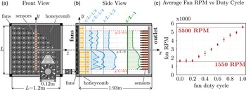
Experimental set-up. (a) Front view of $10\times 10$
fan array, showing the alignment of each sensor (orange circles) along the middle of the array. (b) Fan-array side view, with example velocity profiles at each of the four locations measured along the
$10\times 10$
fan array, showing the alignment of each sensor (orange circles) along the middle of the array. (b) Fan-array side view, with example velocity profiles at each of the four locations measured along the $x$
-axis. The red dashed lines delineate our measurement width. The profile highlighted in green is at our preferred downstream distance,
$x$
-axis. The red dashed lines delineate our measurement width. The profile highlighted in green is at our preferred downstream distance, $x/L=1$
. (c) Steady-state fan RPM as a function of duty cycle, averaged both in time and across all fans. Error bars show one standard deviation above and below. Standard deviations range from 90 RPM at 60 % duty cycle to 220 RPM at 40 % duty cycle, and are 143 RPM on average.
$x/L=1$
. (c) Steady-state fan RPM as a function of duty cycle, averaged both in time and across all fans. Error bars show one standard deviation above and below. Standard deviations range from 90 RPM at 60 % duty cycle to 220 RPM at 40 % duty cycle, and are 143 RPM on average.

For fan-array control, either RPM or duty cycle can be used as the control input. In this work, we choose duty cycle for several reasons. All fans have duty cycle as a control input, but not all have easily accessible RPM feedback. Duty cycle as a prescribed input is noiseless and consistent across all fans, while RPM fluctuates across fan units and is obtained from measurements subject to noise. Moreover, in steady state, the mapping between RPM and duty cycle is linear, as shown in figure 2(c), with the exception of saturation at duty cycles at or below 20 %. This linearity makes the distinction between the two inputs much less significant than when modelling time-varying fan speeds and flow features.
We use one flush-mounted $6.35\,\mathrm{mm}$
diameter,
$6.35\,\mathrm{mm}$
diameter, $38.1\,\mathrm{mm}$
thick ‘honeycomb’ for flow conditioning. We normalise coordinates in the test section by the width of the fan array,
$38.1\,\mathrm{mm}$
thick ‘honeycomb’ for flow conditioning. We normalise coordinates in the test section by the width of the fan array, $L=1.2\,\mathrm{m}$
. This is the same fan-array wind tunnel as used by Fan et al. (Reference Fan, Huertas-Cerdeira, Cossé, Sader and Gharib2019), Sader et al. (Reference Sader, Huertas-Cerdeira and Gharib2016) and Cossé et al. (Reference Cossé, Sader, Kim, Cerdeira and Gharib2014).
$L=1.2\,\mathrm{m}$
. This is the same fan-array wind tunnel as used by Fan et al. (Reference Fan, Huertas-Cerdeira, Cossé, Sader and Gharib2019), Sader et al. (Reference Sader, Huertas-Cerdeira and Gharib2016) and Cossé et al. (Reference Cossé, Sader, Kim, Cerdeira and Gharib2014).
To control our fan array, we partition it into five $2\times 10$
‘modules’, each spanning two rows of the full
$2\times 10$
‘modules’, each spanning two rows of the full $10\times 10$
grid. Each module has one NUCLEO F429ZI microcontroller, which sends the duty-cycle signals and receives the RPM signals of each of its 20 fans. All five microcontrollers are coordinated by a desktop computer over a local area network. Our fan-array control software is available open source (Stefan-Zavala, Reference Stefan-Zavala2023).
$10\times 10$
grid. Each module has one NUCLEO F429ZI microcontroller, which sends the duty-cycle signals and receives the RPM signals of each of its 20 fans. All five microcontrollers are coordinated by a desktop computer over a local area network. Our fan-array control software is available open source (Stefan-Zavala, Reference Stefan-Zavala2023).
2.1.2. Sensor array
We use an array of 17 Sensirion SDP31 digital differential pressure sensors arranged along the spanwise axis ( $y$
) and centred in the middle of our fan array. The 17 sensors are aligned with centres and edges of fans (figure 2
a, b). A detailed description of the sensor array geometry and sensor specifications, including raw time series, is included in the supplementary file. The sensor array is traversed along the streamwise axis (
$y$
) and centred in the middle of our fan array. The 17 sensors are aligned with centres and edges of fans (figure 2
a, b). A detailed description of the sensor array geometry and sensor specifications, including raw time series, is included in the supplementary file. The sensor array is traversed along the streamwise axis ( $x$
), such that profiles are measured at different downstream distances within the
$x$
), such that profiles are measured at different downstream distances within the $z=0$
plane. The pressure sensors are placed in a 3D-printed housing and used as Pitot-static tube anemometers to measure streamwise velocity. All sensors are queried serially using an Adafruit TCA9548A multiplexer. A Teensy 4.0 microcontroller queries the full sensor array at
$z=0$
plane. The pressure sensors are placed in a 3D-printed housing and used as Pitot-static tube anemometers to measure streamwise velocity. All sensors are queried serially using an Adafruit TCA9548A multiplexer. A Teensy 4.0 microcontroller queries the full sensor array at $9.2\ \mathrm{Hz}$
. For a given fan-speed profile, data are collected for 7 s, until statistical convergence, and averaged in time. Since only streamwise velocity is measured, turbulent kinetic energy in the spanwise directions, and thus turbulence intensity, is not available. Instead, we use standard deviation as our measure of error and fluctuation. At
$9.2\ \mathrm{Hz}$
. For a given fan-speed profile, data are collected for 7 s, until statistical convergence, and averaged in time. Since only streamwise velocity is measured, turbulent kinetic energy in the spanwise directions, and thus turbulence intensity, is not available. Instead, we use standard deviation as our measure of error and fluctuation. At $x/L=1$
, samples throughout our dataset have standard deviations ranging from 0.06 to 1.8
$x/L=1$
, samples throughout our dataset have standard deviations ranging from 0.06 to 1.8 $\mathrm{m\,s}^{-1}$
, with an average standard deviation of 0.31
$\mathrm{m\,s}^{-1}$
, with an average standard deviation of 0.31 $\mathrm{m\,s}^{-1}$
. All measured velocity profiles shown in this work, such as in figures 6 and 7 and in supplementary files, show error bars as shaded regions of one standard deviation above and below the mean. Our data collection and processing scripts are implemented using Jupyter Notebook 7.0 (Kluyver et al., Reference Kluyver, Ragan-Kelley, Pérez, Granger, Bussonnier, Frederic, Kelley, Hamrick, Grout, Corlay and Ivanov2016) and the Python 3.11.3 kernel, as well as NumPy version 1.26.4 (Harris et al., Reference Harris, Millman, Van Der Walt, Gommers, Virtanen, Cournapeau, Wieser, Taylor, Berg, Smith and Kern2020), pandas version 2.2.1 (McKinney, Reference McKinney2010) and Matplotlib version 3.8.4. (Hunter, Reference Hunter2007).
$\mathrm{m\,s}^{-1}$
. All measured velocity profiles shown in this work, such as in figures 6 and 7 and in supplementary files, show error bars as shaded regions of one standard deviation above and below the mean. Our data collection and processing scripts are implemented using Jupyter Notebook 7.0 (Kluyver et al., Reference Kluyver, Ragan-Kelley, Pérez, Granger, Bussonnier, Frederic, Kelley, Hamrick, Grout, Corlay and Ivanov2016) and the Python 3.11.3 kernel, as well as NumPy version 1.26.4 (Harris et al., Reference Harris, Millman, Van Der Walt, Gommers, Virtanen, Cournapeau, Wieser, Taylor, Berg, Smith and Kern2020), pandas version 2.2.1 (McKinney, Reference McKinney2010) and Matplotlib version 3.8.4. (Hunter, Reference Hunter2007).
2.1.3. Functional test section: fan-array boundary effects
There are three key boundary effects for the test section of a fan array: close to the array, far from the array and at the spanwise edges of the array. These effects are studied in detail by Veismann et al. (Reference Veismann, Dougherty, Rabinovitch, Quon and Gharib2021
a) and Dougherty (Reference Dougherty2022). When close to the fans (smaller $x/L$
), the effect of fan geometry (the shape of a fan’s hub and the boundary between each fan) is observable in flow profiles, such as in figure 2(b) at
$x/L$
), the effect of fan geometry (the shape of a fan’s hub and the boundary between each fan) is observable in flow profiles, such as in figure 2(b) at $x/L\lt 1$
. With increasing distance from the fans (increasing
$x/L\lt 1$
. With increasing distance from the fans (increasing $x/L$
), artefacts from fan geometry are smoothed by turbulent mixing. However, mixing also dampens the variation introduced by non-uniform fan speeds, which is an essential feature of fan arrays. Measuring too close to the fan array introduces artefacts, measuring too far negates individual fan control. For the fan array used in this paper, we found
$x/L$
), artefacts from fan geometry are smoothed by turbulent mixing. However, mixing also dampens the variation introduced by non-uniform fan speeds, which is an essential feature of fan arrays. Measuring too close to the fan array introduces artefacts, measuring too far negates individual fan control. For the fan array used in this paper, we found $x/L=1$
to be a good trade-off and designate it as our ‘preferred’ downstream distance. The significance of downstream distance, and of our choice of
$x/L=1$
to be a good trade-off and designate it as our ‘preferred’ downstream distance. The significance of downstream distance, and of our choice of $x/L=1$
, is observable in our results and discussed in Sections 3.1.1 and 3.2. For the boundary effects near the spanwise edges of the test section, Veismann et al. (Reference Veismann, Dougherty, Rabinovitch, Quon and Gharib2021
a) recommends, for a fan array with an open test section, testing within
$x/L=1$
, is observable in our results and discussed in Sections 3.1.1 and 3.2. For the boundary effects near the spanwise edges of the test section, Veismann et al. (Reference Veismann, Dougherty, Rabinovitch, Quon and Gharib2021
a) recommends, for a fan array with an open test section, testing within $y/L, z/L \in [-0.4, 0.4]$
to avoid most edge effects. The span of our sensor array, shown in figure 2(b), matches this recommendation. Since no significant increase in unsteadiness, prediction error or tracking error was observed at sensor locations closest to the boundary, we conclude that boundary effects in our enclosed test section are outside the span
$y/L, z/L \in [-0.4, 0.4]$
to avoid most edge effects. The span of our sensor array, shown in figure 2(b), matches this recommendation. Since no significant increase in unsteadiness, prediction error or tracking error was observed at sensor locations closest to the boundary, we conclude that boundary effects in our enclosed test section are outside the span $y/L \in [-0.4, 0.4]$
, and the recommendation of Veismann et al. (Reference Veismann, Dougherty, Rabinovitch, Quon and Gharib2021
a) applies. Note that the fan array used by Veismann et al. (Reference Veismann, Dougherty, Rabinovitch, Quon and Gharib2021
a) has an open test section, while the one used in this work is enclosed. Since boundary layers grow logarithmically with streamwise distance while shear layers grow linearly, we expect the presence of an enclosure to have resulted in a larger functional test section than if the test section were open. However, this hypothesis was not tested, as our measurements did not reach boundary effects. At
$y/L \in [-0.4, 0.4]$
, and the recommendation of Veismann et al. (Reference Veismann, Dougherty, Rabinovitch, Quon and Gharib2021
a) applies. Note that the fan array used by Veismann et al. (Reference Veismann, Dougherty, Rabinovitch, Quon and Gharib2021
a) has an open test section, while the one used in this work is enclosed. Since boundary layers grow logarithmically with streamwise distance while shear layers grow linearly, we expect the presence of an enclosure to have resulted in a larger functional test section than if the test section were open. However, this hypothesis was not tested, as our measurements did not reach boundary effects. At $11\ \mathrm{m\,s}^{-1}$
and
$11\ \mathrm{m\,s}^{-1}$
and $x/L=1$
we expect the boundary-layer thickness of our enclosure to be approximately
$x/L=1$
we expect the boundary-layer thickness of our enclosure to be approximately $3\ \mathrm{cm}$
or
$3\ \mathrm{cm}$
or $y/L\approx 0.0027$
, which is well within the current margin of
$y/L\approx 0.0027$
, which is well within the current margin of $y/L=0.1$
between the sensor array and the enclosure.
$y/L=0.1$
between the sensor array and the enclosure.
2.2. Mathematical methods
2.2.1. Surrogate model
Let ${\boldsymbol{r}}=[r_1,\ r_2,\ \ldots \ r_{N_{\mathrm{fans}}}]$
be a fan-speed profile. Component
${\boldsymbol{r}}=[r_1,\ r_2,\ \ldots \ r_{N_{\mathrm{fans}}}]$
be a fan-speed profile. Component $r_j$
is the duty cycle of the
$r_j$
is the duty cycle of the $j^{\mathrm{}}$
th actuator and is a real-valued scalar ranging from
$j^{\mathrm{}}$
th actuator and is a real-valued scalar ranging from $0$
(minimum fan speed) to
$0$
(minimum fan speed) to $1$
(maximum fan speed). Since we couple each row of fans in our
$1$
(maximum fan speed). Since we couple each row of fans in our $10\times 10$
array to the same duty cycle, we have
$10\times 10$
array to the same duty cycle, we have ${N_{\mathrm{fans}}}=10$
actuators and
${N_{\mathrm{fans}}}=10$
actuators and $r_j$
is the
$r_j$
is the $j^{\mathrm{}}$
th row of fans (figure 2
a). We say
$j^{\mathrm{}}$
th row of fans (figure 2
a). We say $\boldsymbol{r}$
is an input into the fan array.
$\boldsymbol{r}$
is an input into the fan array.
Let $\boldsymbol{v} = [v_1,\ v_2,\ \ldots \ v_{N_{\mathrm{sensors}}}]$
be a velocity profile at a fixed downstream distance. Component
$\boldsymbol{v} = [v_1,\ v_2,\ \ldots \ v_{N_{\mathrm{sensors}}}]$
be a velocity profile at a fixed downstream distance. Component $v_i$
is the non-dimensionalised, time-averaged, streamwise velocity reading of the
$v_i$
is the non-dimensionalised, time-averaged, streamwise velocity reading of the $i^{\mathrm{}}$
th sensor in an array of
$i^{\mathrm{}}$
th sensor in an array of $N_{\mathrm{sensors}}$
sensors, and is a real-valued positive scalar. In this paper, we have
$N_{\mathrm{sensors}}$
sensors, and is a real-valued positive scalar. In this paper, we have ${N_{\mathrm{sensors}}}=17$
sensors along the non-homogeneous spanwise axis
${N_{\mathrm{sensors}}}=17$
sensors along the non-homogeneous spanwise axis $y$
(figure 2
b). We say
$y$
(figure 2
b). We say $\boldsymbol{v}$
is an output of the fan array. A fan-array surrogate model predicts the output
$\boldsymbol{v}$
is an output of the fan array. A fan-array surrogate model predicts the output $\boldsymbol{v}$
produced by a given input
$\boldsymbol{v}$
produced by a given input $\boldsymbol{r}$
.
$\boldsymbol{r}$
.
Let $N_{\mathrm{data}}$
be the number of all experimentally collected profiles at a given downstream distance, each consisting of an input–output pair
$N_{\mathrm{data}}$
be the number of all experimentally collected profiles at a given downstream distance, each consisting of an input–output pair $({\boldsymbol{r}}, \boldsymbol{v})$
. Let
$({\boldsymbol{r}}, \boldsymbol{v})$
. Let ${\boldsymbol{R}}\in [0,1]^{{N_{\mathrm{fans}}}\times N_{\mathrm{data}}}$
be the matrix of
${\boldsymbol{R}}\in [0,1]^{{N_{\mathrm{fans}}}\times N_{\mathrm{data}}}$
be the matrix of $N_{\mathrm{data}}$
horizontally stacked input vectors and
$N_{\mathrm{data}}$
horizontally stacked input vectors and ${\boldsymbol{V}}\in [0,\infty )^{{N_{\mathrm{sensors}}}\times N_{\mathrm{data}}}$
be the matrix of
${\boldsymbol{V}}\in [0,\infty )^{{N_{\mathrm{sensors}}}\times N_{\mathrm{data}}}$
be the matrix of $N$
horizontally stacked output vectors
$N$
horizontally stacked output vectors
 \begin{equation*} \boldsymbol{R} = \begin{bmatrix} | & | & | & & | \\ {\boldsymbol{r}}_1 & {\boldsymbol{r}}_2 & {\boldsymbol{r}}_3 & \ldots & {\boldsymbol{r}}_{N_{\mathrm{data}}} \\ | & | & | & & | \\ \end{bmatrix} \quad \boldsymbol{V} = \begin{bmatrix} | & | & | & & | \\ \boldsymbol{v}_1 & \boldsymbol{v}_2 & \boldsymbol{v}_3 & \ldots & \boldsymbol{v}_{N_{\mathrm{data}}} \\ | & | & | & & | \\ \end{bmatrix}. \end{equation*}
Our surrogate model consists of an ${N_{\mathrm{sensors}}}\times {N_{\mathrm{fans}}}$
coefficient matrix
${N_{\mathrm{sensors}}}\times {N_{\mathrm{fans}}}$
coefficient matrix $\boldsymbol{A}$
and an
$\boldsymbol{A}$
and an $N_{\mathrm{sensors}}$
-dimensional bias vector
$N_{\mathrm{sensors}}$
-dimensional bias vector $\boldsymbol{b}$
. Given an input
$\boldsymbol{b}$
. Given an input $\boldsymbol{r}$
, a prediction
$\boldsymbol{r}$
, a prediction $\boldsymbol{v}_{\mathrm{pred}}$
of the true output
$\boldsymbol{v}_{\mathrm{pred}}$
of the true output $\boldsymbol{v}$
is given by
$\boldsymbol{v}$
is given by
 \begin{equation} \boldsymbol{v}_{\mathrm{pred}} = {\boldsymbol{A}}{\boldsymbol{r}} + {\boldsymbol{b}}. \end{equation}
We produce surrogate model $({\boldsymbol{A}}, {\boldsymbol{b}})$
from data matrices
$({\boldsymbol{A}}, {\boldsymbol{b}})$
from data matrices $\boldsymbol{R}$
and
$\boldsymbol{R}$
and $\boldsymbol{v}$
using regularised linear regression. This means we find the matrix
$\boldsymbol{v}$
using regularised linear regression. This means we find the matrix $\boldsymbol{A}$
and vector
$\boldsymbol{A}$
and vector $\boldsymbol{b}$
that best map
$\boldsymbol{b}$
that best map $\boldsymbol{R}$
to
$\boldsymbol{R}$
to $\boldsymbol{V}$
such that
$\boldsymbol{V}$
such that ${\boldsymbol{A}}{\boldsymbol{R}} + {\boldsymbol{b}} \approx {\boldsymbol{V}}$
. This can be achieved by minimising the
${\boldsymbol{A}}{\boldsymbol{R}} + {\boldsymbol{b}} \approx {\boldsymbol{V}}$
. This can be achieved by minimising the $l_2$
norm of the difference
$l_2$
norm of the difference $||{\boldsymbol{A}}{\boldsymbol{R}} + {\boldsymbol{b}} - {\boldsymbol{V}}||_2$
. To regularise (promote model simplicity), we penalise the
$||{\boldsymbol{A}}{\boldsymbol{R}} + {\boldsymbol{b}} - {\boldsymbol{V}}||_2$
. To regularise (promote model simplicity), we penalise the $\ell _1$
norm of
$\ell _1$
norm of $\boldsymbol{A}$
and
$\boldsymbol{A}$
and $\boldsymbol{b}$
. The explicit form of our regression is
$\boldsymbol{b}$
. The explicit form of our regression is
 \begin{equation} {\boldsymbol{A}},{\boldsymbol{b}} = \underset {{{\boldsymbol{A}},{\boldsymbol{b}}}}{\text{argmin}}\ \ \frac {1}{2N_{\mathrm{data}} }||{\boldsymbol{A}}{\boldsymbol{R}} + {\boldsymbol{b}} - {\boldsymbol{V}}||^2_2 + \alpha (||{\boldsymbol{A}}||_1 + ||{\boldsymbol{b}}||_1). \end{equation}
Penalising the $\ell _1$
-norm of coefficients maximises the number of coefficients set to zero, leading to sparser – and thus simpler – models. For the models presented in this work, we use a regularisation parameter of
$\ell _1$
-norm of coefficients maximises the number of coefficients set to zero, leading to sparser – and thus simpler – models. For the models presented in this work, we use a regularisation parameter of $\alpha =0.01$
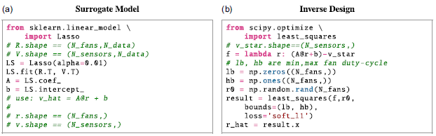
. This parameter was chosen to meet the qualitative sparsity criterion of localised influence near each fan, and resulted in a surrogate model that exceeded our expectations of performance and interpretability given its simplicity, discussed in Sections 3.1 and 3.1.1. Our execution in code is given in figure A1(a) in Appendix A, using Scikit-learn 1.5.1 (Pedregosa et al., Reference Pedregosa, Varoquaux, Gramfort, Michel, Thirion, Grisel, Blondel, Prettenhofer, Weiss, Dubourg and Vanderplas2011).
$\alpha =0.01$
. This parameter was chosen to meet the qualitative sparsity criterion of localised influence near each fan, and resulted in a surrogate model that exceeded our expectations of performance and interpretability given its simplicity, discussed in Sections 3.1 and 3.1.1. Our execution in code is given in figure A1(a) in Appendix A, using Scikit-learn 1.5.1 (Pedregosa et al., Reference Pedregosa, Varoquaux, Gramfort, Michel, Thirion, Grisel, Blondel, Prettenhofer, Weiss, Dubourg and Vanderplas2011).
2.2.2. Inverse design
Given a desired flow profile $\boldsymbol{v}_{\mathrm{target}}$
, we use our surrogate model
$\boldsymbol{v}_{\mathrm{target}}$
, we use our surrogate model $({\boldsymbol{A}},{\boldsymbol{b}})$
within the following quadratic program to find the input
$({\boldsymbol{A}},{\boldsymbol{b}})$
within the following quadratic program to find the input $\hat {\boldsymbol{r}}$
that produces the closest profile to
$\hat {\boldsymbol{r}}$
that produces the closest profile to $\boldsymbol{v}_{\mathrm{target}}$
:
$\boldsymbol{v}_{\mathrm{target}}$
:
 \begin{equation} \begin{aligned} \hat {\boldsymbol{r}}=\underset {{\boldsymbol{r}}}{\mathrm{argmin}} & \frac 12\sum _{i=1}^{N_{\mathrm{sensors}}} \rho \left ((\hat {v}_i({\boldsymbol{r}})-v^\star _i)^2\right )\\ \mathrm{subject\ to} & \\ & {l_k \leq r_k \leq h_k\ \ \forall k\in \{1,\ldots \ {N_{\mathrm{fans}}}\}}\\ \mathrm{where} & \\ & {0 \leq l_k \leq r_k \leq h_k \leq 1}\\ \end{aligned} \end{equation}
where $v_i^\star$
are components of
$v_i^\star$
are components of $\boldsymbol{v}_{\mathrm{target}}$
and
$\boldsymbol{v}_{\mathrm{target}}$
and $\hat {v}_i$
are components of
$\hat {v}_i$
are components of $\boldsymbol{v}_{\mathrm{pred}}={\boldsymbol{A}}{\boldsymbol{r}}+{\boldsymbol{b}}$
. The function
$\boldsymbol{v}_{\mathrm{pred}}={\boldsymbol{A}}{\boldsymbol{r}}+{\boldsymbol{b}}$
. The function $\rho (z)= 2\cdot (\sqrt {1+z} -1)$
is a smooth approximation of the
$\rho (z)= 2\cdot (\sqrt {1+z} -1)$
is a smooth approximation of the $l_1$
norm used in robust least-squares regression and
$l_1$
norm used in robust least-squares regression and $l_k$
and
$l_k$
and $h_k$
are lower and upper bounds on the duty cycle of each fan. The parameters
$h_k$
are lower and upper bounds on the duty cycle of each fan. The parameters $l_k$
and
$l_k$
and $h_k$
encode constraints on the duty cycle, and thus speed, of the
$h_k$
encode constraints on the duty cycle, and thus speed, of the $k^{\text{}}$
th fan in the array, such as saturation (
$k^{\text{}}$
th fan in the array, such as saturation ( $l_k=0, h_k=1$
by default), or ‘dead’ fans (
$l_k=0, h_k=1$
by default), or ‘dead’ fans ( $l_k=h_k=0$
). Here, a dead fan is one constrained to 0 duty cycle, which typically corresponds to 0 RPM, and is equivalent to a fan that has failed and no longer spins. Note this is not the case in our fan array, which has non-zero RPM at 0 duty cycle. Furthermore, in our configuration, where rows of fans are coupled, constraints apply to entire rows of fans, not individual fan units. Our execution in code is given in figure A1(b) in Appendix A, using SciPy 1.12.0 (Virtanen et al., Reference Virtanen, Gommers, Oliphant, Haberland, Reddy, Cournapeau, Burovski, Peterson, Weckesser, Bright and Van Der Walt2020).
$l_k=h_k=0$
). Here, a dead fan is one constrained to 0 duty cycle, which typically corresponds to 0 RPM, and is equivalent to a fan that has failed and no longer spins. Note this is not the case in our fan array, which has non-zero RPM at 0 duty cycle. Furthermore, in our configuration, where rows of fans are coupled, constraints apply to entire rows of fans, not individual fan units. Our execution in code is given in figure A1(b) in Appendix A, using SciPy 1.12.0 (Virtanen et al., Reference Virtanen, Gommers, Oliphant, Haberland, Reddy, Cournapeau, Burovski, Peterson, Weckesser, Bright and Van Der Walt2020).
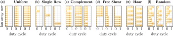
Types of inputs used in dataset. (a) Uniform: same duty cycle for all fans. (b) Single row: one fan row at non-zero duty cycle, all other fans at zero duty cycle. (c) Complement: one fan row at zero duty cycle, all others at non-zero duty cycle. (d) Free shear: top half and bottom half of the fan array at different duty cycles. (e) Haar: concatenated Haar wavelets at different resolutions and their mirror profiles. (f) Random: each fan row at a duty cycle sampled from the uniform distribution $\mathcal{U}[0, 1]$
.
$\mathcal{U}[0, 1]$
.

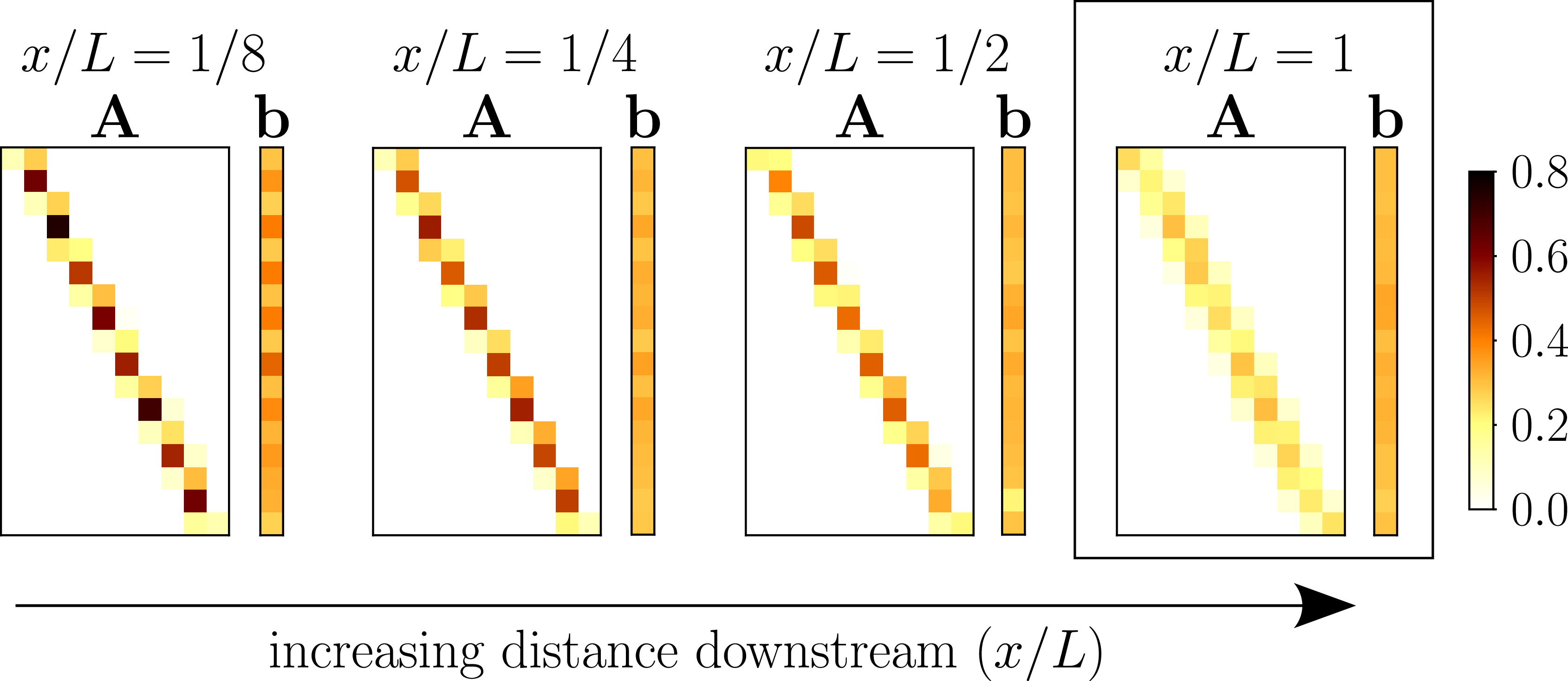
Resulting model matrices $\boldsymbol{A}$
and bias vectors
$\boldsymbol{A}$
and bias vectors $\boldsymbol{b}$
. As
$\boldsymbol{b}$
. As $x/L$
increases, model coefficients appear to ‘diffuse’, discussed in Section 3.1.1. Rightmost: preferred downstream distance
$x/L$
increases, model coefficients appear to ‘diffuse’, discussed in Section 3.1.1. Rightmost: preferred downstream distance $x/L=1$
.
$x/L=1$
.

2.3. Data description
The inputs used for model fitting fall within six types of profiles, described in figure 3. These types were chosen for their relevance in previous fan-array experiments (uniform and free shear), their viability as basis for the fan-array input space (single row and complement) and for broad coverage of the input space (Haar and random). The 169 profiles of the training set are distributed as follows: 11 uniform, 60 single row, 40 complement, 10 free shear, 8 Haar and 40 random. The full training set is visualised in the supplementary file. The resulting models are shown in figure 4 and described in Section 3.1.
To validate our model predictions, we use a set of 63 inputs, split into two parts. The first part of the test set consists of 29 profiles of, with one exception, the same types as those used in the training set. They are distributed as follows: 4 uniform, 6 single row, 4 free shear, 5 random and 10 sparse random. Sparse random profiles, which are not present in the training set, are given by $r_k=\mathrm{dc}\cdot \lfloor s\rfloor$
,
$r_k=\mathrm{dc}\cdot \lfloor s\rfloor$
, $k\in \{1,\ldots \ {N_{\mathrm{fans}}}\}$
with
$k\in \{1,\ldots \ {N_{\mathrm{fans}}}\}$
with $\mathrm{dc}\in \{0.5, 1\}$
and
$\mathrm{dc}\in \{0.5, 1\}$
and $s\sim \mathcal{U}[0,1]$
. The second part of the prediction test set consists of inputs produced by the inverse-design scheme. A set of target velocities was produced using the same process as our input datasets, but using vectors of size
$s\sim \mathcal{U}[0,1]$
. The second part of the prediction test set consists of inputs produced by the inverse-design scheme. A set of target velocities was produced using the same process as our input datasets, but using vectors of size $N_{\mathrm{sensors}}$
instead of
$N_{\mathrm{sensors}}$
instead of $N_{\mathrm{fans}}$
, and with a minimum value of
$N_{\mathrm{fans}}$
, and with a minimum value of $0.3\ V_{\text{max}}$
to account for the fan array’s minimum wind speed. This part is distributed as follows: 6 uniform, 4 free shear, 9 single row, 5 random and 10 sparse random. Fan row 4 was constrained to 0 duty cycle by setting
$0.3\ V_{\text{max}}$
to account for the fan array’s minimum wind speed. This part is distributed as follows: 6 uniform, 4 free shear, 9 single row, 5 random and 10 sparse random. Fan row 4 was constrained to 0 duty cycle by setting $h_4=0.01$
in equation (3). The fan-speed profiles produced by our inverse-design scheme to approximate the target velocity profiles in this set were then used as part of the prediction test set. Both the inverse-design fan speeds and the sparse random category were introduced to further gauge generalisation by testing on profiles generated from a substantially different process as those seen in training. The full prediction test set is visualised in the supplementary file. Prediction performance is described in Section 3.2.
$h_4=0.01$
in equation (3). The fan-speed profiles produced by our inverse-design scheme to approximate the target velocity profiles in this set were then used as part of the prediction test set. Both the inverse-design fan speeds and the sparse random category were introduced to further gauge generalisation by testing on profiles generated from a substantially different process as those seen in training. The full prediction test set is visualised in the supplementary file. Prediction performance is described in Section 3.2.
We validate the tracking performance of our inverse-design scheme using a set of 37 target velocity profiles, distributed as follows: 5 uniform, 6 free shear, 5 random, 3 sparse random, 2 parabolic and 17 profiles taken from slicing an arbitrary two-dimensional image. Parabolic profiles draw a parabola matching Poiseuille flow, as shown in figure 7(d). The full inverse-design test set is visualised in the supplementary file. Tracking performance is described in Section 3.3.
3. Results
3.1. Surrogate model
A surrogate model $({\boldsymbol{A}}, {\boldsymbol{b}})$
(Section 2.2.1) was fit on training datasets for each of the four measured locations
$({\boldsymbol{A}}, {\boldsymbol{b}})$
(Section 2.2.1) was fit on training datasets for each of the four measured locations $x/L\in \{1/8, 1/4,1/2,1\}$
(Section 2.3). The resulting model coefficients and biases are shown in figure 4. According to the model coefficients, each sensor reading (row of
$x/L\in \{1/8, 1/4,1/2,1\}$
(Section 2.3). The resulting model coefficients and biases are shown in figure 4. According to the model coefficients, each sensor reading (row of $\boldsymbol{A}$
) is primarily affected by the speed of fans (columns of
$\boldsymbol{A}$
) is primarily affected by the speed of fans (columns of $\boldsymbol{A}$
) directly upstream, is secondarily affected by adjacent fans and is insensitive to all other fans. This is encoded in the tri-diagonal-like structure of
$\boldsymbol{A}$
) directly upstream, is secondarily affected by adjacent fans and is insensitive to all other fans. This is encoded in the tri-diagonal-like structure of $\boldsymbol{A}$
. The average
$\boldsymbol{A}$
. The average $R^2$
value across all 17 output variables is lowest at
$R^2$
value across all 17 output variables is lowest at $x/L=1/8$
with
$x/L=1/8$
with $R^2=0.74$
, highest at
$R^2=0.74$
, highest at $x/L=1/2$
with
$x/L=1/2$
with $R^2=0.81$
and is
$R^2=0.81$
and is $R^2=0.79$
at
$R^2=0.79$
at $x/L=1$
. These
$x/L=1$
. These $R^2$
values suggest most of the variation in sensor readings is explained by a linear map, and increasingly so with
$R^2$
values suggest most of the variation in sensor readings is explained by a linear map, and increasingly so with $x/L$
.
$x/L$
.
3.1.1. Physical interpretation of model coefficients
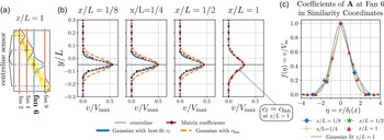
To interpret our model, we compare it with a superposition of time-averaged round jets centred on each fan. We find that the coefficients of each matrix column match the canonical profile of time-averaged streamwise velocity of a round jet. The centreline of each column’s ‘jet’ is aligned with the axis of the fan whose speed multiplies that column. We approximate this jet profile by fitting a Gaussian of the form
 \begin{equation} g(r)=V_m\exp \left (-\frac {r^2}{2c^2}\right ) \quad \text{where}\ r = \frac {y-y_m}{L} \end{equation}
on the coefficients of each matrix column. Here, $y_m$
is the spanwise coordinate of the jet centreline,
$y_m$
is the spanwise coordinate of the jet centreline, $c$
is a free parameter and
$c$
is a free parameter and $V_m$
is the centreline velocity, which is assigned the model coefficient aligned with the fan centre. We show Gaussian fits for several matrix columns at
$V_m$
is the centreline velocity, which is assigned the model coefficient aligned with the fan centre. We show Gaussian fits for several matrix columns at $x/L=1$
in figure 5(a). For this analysis, we will focus on one column, column 6, of the model matrix, which corresponds to the 6th row of fans in the array. As shown in figure 5(b), we fit two Gaussian profiles, one with
$x/L=1$
in figure 5(a). For this analysis, we will focus on one column, column 6, of the model matrix, which corresponds to the 6th row of fans in the array. As shown in figure 5(b), we fit two Gaussian profiles, one with $c=c_l$
optimised for best fit, and another with
$c=c_l$
optimised for best fit, and another with $c=c_{\mathrm{fan}}=d/L$
, where
$c=c_{\mathrm{fan}}=d/L$
, where $d$
is the fan diameter. The best-fit profile fits the matrix coefficients well for all
$d$
is the fan diameter. The best-fit profile fits the matrix coefficients well for all $x/L$
, but the fan-diameter profile matches the matrix coefficients only at
$x/L$
, but the fan-diameter profile matches the matrix coefficients only at $x/L=1$
. That is, the learned characteristic length scale of our model converges to fan diameter at our preferred downstream distance. Lastly, the matrix coefficients of column 6 for all
$x/L=1$
. That is, the learned characteristic length scale of our model converges to fan diameter at our preferred downstream distance. Lastly, the matrix coefficients of column 6 for all $x/L$
collapse together under the similarity transformation given by
$x/L$
collapse together under the similarity transformation given by $f(\eta )=v/V_m$
,
$f(\eta )=v/V_m$
, $\eta =r/\delta _l$
, where
$\eta =r/\delta _l$
, where $\delta _l$
is the distance from the centreline at which
$\delta _l$
is the distance from the centreline at which $g(\delta _l)=V_m/2$
(figure 5
c). This means the streamwise evolution of model coefficients is self-similar under the same transformation as a canonical round jet (Bailly & Comte-Bellot, Reference Bailly, Comte-Bellot, Bailly and Comte-Bellot2015).
$g(\delta _l)=V_m/2$
(figure 5
c). This means the streamwise evolution of model coefficients is self-similar under the same transformation as a canonical round jet (Bailly & Comte-Bellot, Reference Bailly, Comte-Bellot, Bailly and Comte-Bellot2015).
The bias vector, aside from modelling the non-zero velocity floor at minimum RPM, captured imperfections such as the effect of fan geometry – observable as the ‘periodic’ pattern in its coefficients at $x/L\lt 0.5$
in figure 4 – and the aggregate error in fan RPM and sensor reading that is not offset by our calibration process. The latter effect is evident when a column of coefficients of
$x/L\lt 0.5$
in figure 4 – and the aggregate error in fan RPM and sensor reading that is not offset by our calibration process. The latter effect is evident when a column of coefficients of $\boldsymbol{A}$
is plotted without adding
$\boldsymbol{A}$
is plotted without adding $\boldsymbol{b}$
, in this case the coefficients draw symmetric peaks with completely flat tails. This effect is shown in separate plots of model matrix column, bias vector and their sum in the supplementary file.
$\boldsymbol{b}$
, in this case the coefficients draw symmetric peaks with completely flat tails. This effect is shown in separate plots of model matrix column, bias vector and their sum in the supplementary file.
Our model is effectively superimposing round-jet profiles centred on each fan. (a) Gaussian profiles are fit to columns of the model matrix. Column 6 is used in the rest of this figure. (b) Coefficients of column 6 of $\boldsymbol{A}$
and Gaussian fits using best-fit (
$\boldsymbol{A}$
and Gaussian fits using best-fit ( $c_l$
, blue) and fan-diameter (
$c_l$
, blue) and fan-diameter ( $c_{\mathrm{fan}}$
, orange) length scales. Both Gaussian fits converge at
$c_{\mathrm{fan}}$
, orange) length scales. Both Gaussian fits converge at $x/L=1$
. (c) Column 6 of
$x/L=1$
. (c) Column 6 of $\boldsymbol{A}$
for all
$\boldsymbol{A}$
for all $x/L$
plotted in similarity coordinates.
$x/L$
plotted in similarity coordinates.

3.2. Output prediction
Out-of-sample (not seen in training) prediction performance was tested on $63$
fan-array inputs at each
$63$
fan-array inputs at each $x/L$
(Section 2.3). We quantify prediction error as mean absolute error (MAE) between measured and predicted profiles. For a single input
$x/L$
(Section 2.3). We quantify prediction error as mean absolute error (MAE) between measured and predicted profiles. For a single input $\boldsymbol{r}$
, prediction
$\boldsymbol{r}$
, prediction $\boldsymbol{v}_{\mathrm{pred}} = {\boldsymbol{A}}{\boldsymbol{r}} + {\boldsymbol{b}}$
and true measurement
$\boldsymbol{v}_{\mathrm{pred}} = {\boldsymbol{A}}{\boldsymbol{r}} + {\boldsymbol{b}}$
and true measurement $\boldsymbol{v}_{\mathrm{true}}$
, the prediction error of this one sample is the average absolute value of the component-wise difference between
$\boldsymbol{v}_{\mathrm{true}}$
, the prediction error of this one sample is the average absolute value of the component-wise difference between $\boldsymbol{v}_{\mathrm{true}} - \boldsymbol{v}_{\mathrm{pred}}$
 \begin{equation} \mathrm{MAE}(\boldsymbol{v}_{\mathrm{true}}, \boldsymbol{v}_{\mathrm{pred}}) = \frac {1}{N_{\mathrm{sensors}}}\sum _k^{N_{\mathrm{sensors}}} |v_k - \hat {v}_k| \quad \quad \begin{matrix} \boldsymbol{v}_{\mathrm{true}} = [v_1,v_2,\ldots v_k,\ldots v_{N_{\mathrm{sensors}}}]^{\mathrm{T}}, \\ \boldsymbol{v}_{\mathrm{pred}} = [\hat {v}_1,\hat {v}_2,\ldots \hat {v}_k, \ldots \hat {v}_{N_{\mathrm{sensors}}}]^{\mathrm{T}}.\end{matrix} \end{equation}
The prediction error for an entire dataset is the average of all sample-wise MAEs. Since our profiles are normalised by $V_{\mathrm{max}}=11\ \text{m s}^{-1}$
, this MAE is in non-dimensional velocity as a fraction of
$V_{\mathrm{max}}=11\ \text{m s}^{-1}$
, this MAE is in non-dimensional velocity as a fraction of $V_{\mathrm{max}}$
. Multiplying by
$V_{\mathrm{max}}$
. Multiplying by $V_{\mathrm{max}}$
gives the dimensional MAEs reported in this section.
$V_{\mathrm{max}}$
gives the dimensional MAEs reported in this section.
At the preferred downstream distance $x/L=1$
, testing MAE is 0.093
$x/L=1$
, testing MAE is 0.093 $v_{\mathrm{error}}/V_{\mathrm{max}}$
or
$v_{\mathrm{error}}/V_{\mathrm{max}}$
or $1.02\ \mathrm{m\,s}^{-1}$
and training MAE is 0.057
$1.02\ \mathrm{m\,s}^{-1}$
and training MAE is 0.057 $v_{\mathrm{error}}/V_{\mathrm{max}}$
or 0.63 m s−1. This performance is consistent across downstream distances: the additional distances
$v_{\mathrm{error}}/V_{\mathrm{max}}$
or 0.63 m s−1. This performance is consistent across downstream distances: the additional distances $x/L\in \{1/2,1/4,1/8\}$
have dimensional testing MAEs of 1.04, 1.06 and 1.16 m s−1, respectively, and dimensional training MAEs of 0.61, 0.72 and 0.86 m s−1, respectively. This gives an average out-of-sample (test-set) prediction error of 1.07 m s−1 across all measured
$x/L\in \{1/2,1/4,1/8\}$
have dimensional testing MAEs of 1.04, 1.06 and 1.16 m s−1, respectively, and dimensional training MAEs of 0.61, 0.72 and 0.86 m s−1, respectively. This gives an average out-of-sample (test-set) prediction error of 1.07 m s−1 across all measured $x/L$
.
$x/L$
.
Example profiles from flow prediction test set. Sample-wise mean absolute per cent error (MAPE) $E_P$
is shown above each sample. (a)–(d) Test-set profiles at
$E_P$
is shown above each sample. (a)–(d) Test-set profiles at $x/L=1$
, showing input profile, model prediction and true measurement. (e) Test-set profiles of the same input at all modelled downstream distances. (f) Kernel-density plots showing the distribution of component-wise (signed) prediction errors (
$x/L=1$
, showing input profile, model prediction and true measurement. (e) Test-set profiles of the same input at all modelled downstream distances. (f) Kernel-density plots showing the distribution of component-wise (signed) prediction errors ( $v-\hat {v}$
) for both train and test set.
$v-\hat {v}$
) for both train and test set.

We additionally compute mean absolute percentage error (MAPE), which normalises the component-wise error by the absolute value of the $\boldsymbol{v}_{\mathrm{true}}$
component
$\boldsymbol{v}_{\mathrm{true}}$
component
 \begin{equation} \mathrm{MAPE}(\boldsymbol{v}_{\mathrm{true}}, \boldsymbol{v}_{\mathrm{pred}}) = \frac {1}{N_{\mathrm{sensors}}}\sum _k^{N_{\mathrm{sensors}}} \frac {|v_k - \hat {v}_k|}{\max (|v_k|, \epsilon )} \quad \begin{matrix} \boldsymbol{v}_{\mathrm{true}} = [v_1,v_2,\ldots v_k,\ldots v_{N_{\mathrm{sensors}}}]^{\mathrm{T}}, \\ \boldsymbol{v}_{\mathrm{pred}} = [\hat {v}_1,\hat {v}_2,\ldots \hat {v}_k, \ldots \hat {v}_{N_{\mathrm{sensors}}}]^{\mathrm{T}}. \end{matrix} \end{equation}
Here, $\epsilon$
is an arbitrary, small constant used to prevent division by zero. At the preferred downstream distance
$\epsilon$
is an arbitrary, small constant used to prevent division by zero. At the preferred downstream distance $x/L=1$
, training and testing MAPEs are 0.132 (13 %) and 0.173 (17.3 %), respectively. The additional distances
$x/L=1$
, training and testing MAPEs are 0.132 (13 %) and 0.173 (17.3 %), respectively. The additional distances $x/L\in \{1/8, 1/4, 1/2\}$
have training MAPEs of 0.158, 0.146, 0.126, and testing MAPEs of 0.186, 0.176, 0.164, respectively. Highlighted samples from testing and their individual MAPEs are shown in figure 6.
$x/L\in \{1/8, 1/4, 1/2\}$
have training MAPEs of 0.158, 0.146, 0.126, and testing MAPEs of 0.186, 0.176, 0.164, respectively. Highlighted samples from testing and their individual MAPEs are shown in figure 6.
Kernel-density plots of signed, component-wise error distributions ( $v_{\mathrm{true}}-v_{\mathrm{pred}}$
) at
$v_{\mathrm{true}}-v_{\mathrm{pred}}$
) at $x/L=1$
, shown in figure 6(f), show a bias towards positive error or undershooting (
$x/L=1$
, shown in figure 6(f), show a bias towards positive error or undershooting ( $v_{\mathrm{pred}} \lt v_{\mathrm{true}}$
), stronger in testing than in training. This pattern is observable in all samples shown in figure 6(a–e), where most errors (red shade) consist of measured profiles (green crosses) being larger (to the right) than predicted profiles (blue diamonds). Sample-wise error for the full training and test sets is plotted in the supplementary file.
$v_{\mathrm{pred}} \lt v_{\mathrm{true}}$
), stronger in testing than in training. This pattern is observable in all samples shown in figure 6(a–e), where most errors (red shade) consist of measured profiles (green crosses) being larger (to the right) than predicted profiles (blue diamonds). Sample-wise error for the full training and test sets is plotted in the supplementary file.
We attribute error outside of standard deviation and sensor noise to nonlinear flow effects, such as entrainment and turbulent mixing, which are characteristic of turbulent flows with significant spatial velocity gradients. This pattern is visible in figure 6(a–e), where the largest discrepancies between model and measurement exist near are commensurate with larger changes in duty cycle and thus RPM and inlet-flow speed. The test cases for $x/L\lt 1$
shown in figure 6(e) further illustrate our choice of
$x/L\lt 1$
shown in figure 6(e) further illustrate our choice of $x/L=1$
as preferred downstream distance. While the only difference between models for different distances is how close to the array flow was measured, prediction performance noticeably worsens with decreasing
$x/L=1$
as preferred downstream distance. While the only difference between models for different distances is how close to the array flow was measured, prediction performance noticeably worsens with decreasing $x/L$
. At
$x/L$
. At $x/L=1$
, the predicted profile is almost entirely within error bounds of the measured profile. The MAPE (labelled
$x/L=1$
, the predicted profile is almost entirely within error bounds of the measured profile. The MAPE (labelled $E_P$
, shown above each profile) at
$E_P$
, shown above each profile) at $x/L=1/4$
and
$x/L=1/4$
and $x/L=1/8$
is almost twice that at
$x/L=1/8$
is almost twice that at $x/L=1$
. Most notably, the visible ‘peaks’ at
$x/L=1$
. Most notably, the visible ‘peaks’ at $x/L\lt 1$
match fan geometry. At all measured locations closer than our preferred distance, fan geometry introduces significant complexity to the flow that is an artefact of our facility, not an outcome of flow prescription.
$x/L\lt 1$
match fan geometry. At all measured locations closer than our preferred distance, fan geometry introduces significant complexity to the flow that is an artefact of our facility, not an outcome of flow prescription.
3.3. Inverse design
Tracking performance of the inverse-design open-loop control algorithm described in Section 2.2.2 was tested at the preferred downstream distance $x/L=1$
using a set of 37 target velocity profiles not present in the model testing or training datasets.
$x/L=1$
using a set of 37 target velocity profiles not present in the model testing or training datasets.
Example profiles from inverse-design validation at $x/L=1$
. (a)–(d) Resulting control input (yellow), target flow (green) and resulting measured profile (blue). Sample-wise MAPE
$x/L=1$
. (a)–(d) Resulting control input (yellow), target flow (green) and resulting measured profile (blue). Sample-wise MAPE $E_P$
is shown above each sample. (e) Kernel-density plot of the distribution of (signed) component-wise tracking error (
$E_P$
is shown above each sample. (e) Kernel-density plot of the distribution of (signed) component-wise tracking error ( $v_{\mathrm{target}} - v$
), along with prediction error for inverse-design inputs, and prediction test error from figure 6.
$v_{\mathrm{target}} - v$
), along with prediction error for inverse-design inputs, and prediction test error from figure 6.

We quantify tracking error the same way as prediction error in Section 3.2, as the MAE between a target velocity profile $\boldsymbol{v}_{\mathrm{target}}$
and the measured velocity profile
$\boldsymbol{v}_{\mathrm{target}}$
and the measured velocity profile $\boldsymbol{v}_{\mathrm{measured}}$
that results from executing the fan-array input
$\boldsymbol{v}_{\mathrm{measured}}$
that results from executing the fan-array input $\boldsymbol{\hat {r}}$
produced by the inverse-design algorithm to track
$\boldsymbol{\hat {r}}$
produced by the inverse-design algorithm to track $\boldsymbol{v}_{\mathrm{target}}$
, the tracking error of a single sample is given by
$\boldsymbol{v}_{\mathrm{target}}$
, the tracking error of a single sample is given by $\mathrm{MAE}(\boldsymbol{v}_{\mathrm{target}},\boldsymbol{v}_{\mathrm{measured}})$
in equation (5). The tracking error of the entire inverse-design test dataset is the average of all sample-wise tracking errors. The
$\mathrm{MAE}(\boldsymbol{v}_{\mathrm{target}},\boldsymbol{v}_{\mathrm{measured}})$
in equation (5). The tracking error of the entire inverse-design test dataset is the average of all sample-wise tracking errors. The $x/L=1$
inverse-design test set has a normalised MAE of 0.095
$x/L=1$
inverse-design test set has a normalised MAE of 0.095 $v_{\mathrm{error}}/V_{\mathrm{max}}$
and a MAPE of 0.215. This gives an average dimensional tracking error of 1.05 m s−1 for
$v_{\mathrm{error}}/V_{\mathrm{max}}$
and a MAPE of 0.215. This gives an average dimensional tracking error of 1.05 m s−1 for $x/L=1$
. Test-set prediction MAE for
$x/L=1$
. Test-set prediction MAE for $x/L=1$
is 1.02 m s−1 (Section 3.2). The MAE suggests the inverse-design open-loop control algorithm is as effective at tracking target profiles as the underlying linear model is at predicting profiles, if slightly worse at lower velocities, as suggested by higher MAPE. This consistency in performance between tracking and prediction is visible in figure 7(e).
$x/L=1$
is 1.02 m s−1 (Section 3.2). The MAE suggests the inverse-design open-loop control algorithm is as effective at tracking target profiles as the underlying linear model is at predicting profiles, if slightly worse at lower velocities, as suggested by higher MAPE. This consistency in performance between tracking and prediction is visible in figure 7(e).
Comparing the distribution of signed tracking errors in figure 7(e) shows complementary biases: prediction error is biased towards underestimating outputs and tracking error is, in turn, biased towards overshooting targets. The profiles in figure 7(a–d) show this overshoot, where measured profiles (blue diamonds) are most often of larger magnitude (to the right) of target profiles (green crosses). As with prediction error in Section 3.2, we attribute tracking error outside standard deviation to nonlinear fluid-dynamic effects that cannot be captured by a linear map, most evident in figure 7(c–d).
4. Discussion and conclusion
Several trends in our results support the choice of $x/L=1$
as preferred downstream location. Model fit quality measured as
$x/L=1$
as preferred downstream location. Model fit quality measured as $R^2$
-score grows from 0.74 at
$R^2$
-score grows from 0.74 at $x/L=1/8$
to 0.79 at
$x/L=1/8$
to 0.79 at $x/L=1$
. Prediction test error as MAPE shrinks from 18.6 % at
$x/L=1$
. Prediction test error as MAPE shrinks from 18.6 % at $x/L=1/8$
to 17.3 % at
$x/L=1/8$
to 17.3 % at $x/L=1$
. Most importantly, artefacts from fan geometry go from a dominant flow feature at
$x/L=1$
. Most importantly, artefacts from fan geometry go from a dominant flow feature at $x/L=1/8$
to negligible at
$x/L=1/8$
to negligible at $x/L=1$
. These results, however, do not set
$x/L=1$
. These results, however, do not set $x/L=1$
decisively as the best possible location for this fan array. The
$x/L=1$
decisively as the best possible location for this fan array. The $R^2$
score and prediction test error are marginally better at
$R^2$
score and prediction test error are marginally better at $x/L=1/2$
, at 0.81 and 16.4 % respectively. Though fan geometry is noticeable at
$x/L=1/2$
, at 0.81 and 16.4 % respectively. Though fan geometry is noticeable at $x/L=1/2$
, making
$x/L=1/2$
, making $x/L=1$
still preferable. It is possible that the optimal location for this fan array lies somewhere between
$x/L=1$
still preferable. It is possible that the optimal location for this fan array lies somewhere between $x/L=1/2$
and
$x/L=1/2$
and $x/L=1$
. Another result highlighting the
$x/L=1$
. Another result highlighting the $x/L=1$
location is the convergence of the learned jet-profile length scale to the width of our fans. Though we find this convergence to be a noteworthy result on its own, further investigation is needed to assign practical implications.
$x/L=1$
location is the convergence of the learned jet-profile length scale to the width of our fans. Though we find this convergence to be a noteworthy result on its own, further investigation is needed to assign practical implications.
A more immediate implication of our jet-superposition interpretation is that resolving the profiles of each individual fan is enough to linearly model the mean flow of the entire fan array. We briefly tested this hypothesis by fitting a model on subsets of the $x/L=1$
training set. Using only uniform and single-row profiles resulted in a test-set prediction MAPE of 21.4 %. Fitting on uniform, single-row and single-row complement profiles resulted in 18.3 % MAPE. Compare these errors with 17.3 % MAPE on the full dataset. All three models are visually indistinguishable. This result suggests that most linear model convergence is obtained from fitting on uniform and single-row profiles alone. Since one of the essential challenges of fan-array modelling is the intractable number of possible fan-speed combinations, finding a minimal set of profiles to produce a working model is a significant practical development. Moreover, by characterising the self-similar streamwise development of model coefficients, their values at streamwise locations between measurements can be interpolated, so a few measurement locations can be used to fill in the entire streamwise length. Finally, since our fan array is the same along both
$x/L=1$
training set. Using only uniform and single-row profiles resulted in a test-set prediction MAPE of 21.4 %. Fitting on uniform, single-row and single-row complement profiles resulted in 18.3 % MAPE. Compare these errors with 17.3 % MAPE on the full dataset. All three models are visually indistinguishable. This result suggests that most linear model convergence is obtained from fitting on uniform and single-row profiles alone. Since one of the essential challenges of fan-array modelling is the intractable number of possible fan-speed combinations, finding a minimal set of profiles to produce a working model is a significant practical development. Moreover, by characterising the self-similar streamwise development of model coefficients, their values at streamwise locations between measurements can be interpolated, so a few measurement locations can be used to fill in the entire streamwise length. Finally, since our fan array is the same along both $y$
and
$y$
and $z$
spanwise directions, we expect the methodology of this work to be as effective in a ‘two-dimensional’ fan array in which fan rows are decoupled as it is in our ‘one-dimensional’ case. If the relationship between the jet-profiles of fans at different spanwise locations is modelled, the profiles of all fans can be inferred from characterising a single one.
$z$
spanwise directions, we expect the methodology of this work to be as effective in a ‘two-dimensional’ fan array in which fan rows are decoupled as it is in our ‘one-dimensional’ case. If the relationship between the jet-profiles of fans at different spanwise locations is modelled, the profiles of all fans can be inferred from characterising a single one.
The hypotheses discussed so far suggest the following process: (i) a single fan’s jet profile is measured at a few streamwise locations, (ii) the self-similar jet-profiles for all streamwise locations are interpolated and (iii) the jet profiles of all fans (in both spanwise axes) are inferred from the one obtained through measurement and interpolation. This process would produce a surrogate model for the mean flow in the entire three-dimensional test section of a fan array given only the profile of a single fan at a few locations.
Our surrogate model’s out-of-sample MAPE of 17.3 % and $R^2$
value of 0.79 at
$R^2$
value of 0.79 at $x/L=1$
suggest the map from steady fan-array speeds to time-averaged streamwise velocities is dominantly linear. However, comparing the mean absolute prediction test error of 1.02 m s−1 with the standard deviation of the sensor readings, which is 0.31 m s−1 on average, suggests that a nonlinear extension of the surrogate model would further improve prediction and tracking. This extension can be implemented such that the resulting model is still easily interpretable, such as by introducing nonlinear functions of fan speeds as additional input features to a regularised linear map. In addition to a nonlinear extension, there are flow quantities of interest other than streamwise velocity, such as spanwise velocity components, turbulence intensity and frequency content. For each of these quantities we expect a regularised linear map to be, if not a sufficient model on its own, a useful, principled baseline.
$x/L=1$
suggest the map from steady fan-array speeds to time-averaged streamwise velocities is dominantly linear. However, comparing the mean absolute prediction test error of 1.02 m s−1 with the standard deviation of the sensor readings, which is 0.31 m s−1 on average, suggests that a nonlinear extension of the surrogate model would further improve prediction and tracking. This extension can be implemented such that the resulting model is still easily interpretable, such as by introducing nonlinear functions of fan speeds as additional input features to a regularised linear map. In addition to a nonlinear extension, there are flow quantities of interest other than streamwise velocity, such as spanwise velocity components, turbulence intensity and frequency content. For each of these quantities we expect a regularised linear map to be, if not a sufficient model on its own, a useful, principled baseline.
Supplementary material
The supplementary material for this article can be found at https://doi.org/10.1017/flo.2025.10034. Code supplement available at https://github.com/astefanz/fml-1.
Acknowledgements
A.S.Z. Acknowledges Amrita Mayavaram and Peter Renn for the development of the anemometers used in data collection; Maya Madere for the wiring and assembly of the initial sensor array; Noel Esparza-Duran for the reassembly and restoration of the first and second fan arrays used; Chris Dougherty, Marcel Veismann and David Kremers for their mentorship and initial conceptualisation of fan-array modelling and control; Peter Crocker and Steve Madere for discussions leading to instrumental insights; as well as family, friends and colleagues – especially Samm Crocker, Jack Caldwell, Julian Humml, Michael Ol and Ariane Mora – for their support. Acknowledgement hash: 27d64cb5a58c7f2057a0ebf1979a975ce99a042aaf182a7f52c24f63859048ca
Data availability statement
Raw data are available from the corresponding author A.S.Z., upon reasonable request.
Author contributions
Conceptualisation: A.S.Z., S.L.B., I.M.; data collection – proof-of-concept: A.S.Z., I.M.; data collection – for publication: A.S.Z., I.S.; formal analysis: A.S.Z., I.S., S.L.B.; visualisation: A.S.Z., I.S., S.L.B.; funding acquisition: M.G.; supervision: I.S., S.L.B., M.G.; writing – original draft: A.S.Z; writing – review and editing: A.S.Z., I.S., S.L.B., I.M.
Funding statement
S.L.B. acknowledges funding support from the Air Force Office of Scientific Research (FA9550-21-1-0178).
Declaration of interests
The authors declare no conflict of interest.
Ethical standards
The research meets all ethical guidelines, including adherence to the legal requirements of the study country.
Appendix A. Code snippets
Execution of mathematical methods in Python 3. (a) Regression of surrogate model given input dataset $\boldsymbol{R}$
and output dataset
$\boldsymbol{R}$
and output dataset $\boldsymbol{V}$
. (b) Inverse-design application of the surrogate model to estimate the best input
$\boldsymbol{V}$
. (b) Inverse-design application of the surrogate model to estimate the best input $\hat {\boldsymbol{r}}$
for a desired profile
$\hat {\boldsymbol{r}}$
for a desired profile $\boldsymbol{v}_{\mathrm{target}}$
.
$\boldsymbol{v}_{\mathrm{target}}$
.











 Open access

