2. How the pooled estimator weights experiments

Consider a case where it is appropriate to estimate the effect of treatment condition $x_{e,i,t}$ on outcome variable $y_{e,i,t}$ using linear regression, where $e$, $i$, and $t$ index the experiment, participant, and decision, respectively. That is, we wish to estimate the parameter $\beta_1$ in the following equation:

\begin{equation*} y_{e,i,t}=\beta_0+\beta_1x_{e,i,t}+\epsilon_{e,i,t} \end{equation*}

where $e$ indexes the experiment, $i$ the participant, and $t$ the decision.

Since in each experiment the treatment is assigned randomly, we have an unbiased estimator for the treatment effect $\beta_1$ for every experiment that has some variation in the treatment variable:

\begin{equation*} \hat\beta_{1}^e=\frac{\sum_{\forall i,t\in e}(y_{e,i,t}-\bar y_e)(x_{e,i,t}-\bar x_e)}{\sum_{\forall i,t\in e}(x_{e,i,t}-\bar x_e)^2} \end{equation*}

where $\bar y_e$ and $\bar x_e$ are the means within experiment $e$ of $y$ and $x$, respectively. $\hat\beta_1^e$ is the within-experiment estimator, because it identifies treatment effects due to variation in $x_{e,i,t}$ within an experiment only. Presumably, the realization of $\hat\beta^e_1$ is the estimate of the treatment effect that is reported in experiment $e$.

Now consider pooling all of the experiments in the meta-study, and again estimating $\beta_1$ using OLS. In this case, we can write this pooled estimator as (see Appendix A for a derivation):

(1)\begin{equation} \hat\beta_1^\text{pooled}=\sum_{\forall e}w_e\hat\beta_1^e+ \left(1-\sum_{\forall e}w_e\right)\tilde\beta_1 \end{equation}

(2)\begin{equation} \text{where: } w_e=\frac{\sum_{\forall i,t\in e}(x_{e,i,t}-\bar x_e)^2}{\sum_{\forall e}\sum_{\forall i,t\in e}(x_{e,i,t}-\bar x_e)^2+\sum_{\forall e}\sum_{\forall i,t\in e}(\bar x_{e}-\bar x)^2} \end{equation}

(3)\begin{equation} \tilde\beta_1=\frac{\sum_{\forall e}\sum_{\forall i,t\in e}(\bar y_e-\bar y)(\bar x_e-\bar x)}{\sum_{\forall e}\sum_{\forall i,t\in e}(\bar x_e-\bar x)^2} \end{equation}

where $\bar y$ and $\bar x$ are the sample means of $y_{e,i,t}$ and $x_{e,i,t}$ over the entire dataset.Footnote ² Note that $\hat\beta_1^\text{pooled}$ is a weighted sum of (i) the experiment-specific estimators $\hat\beta^e_1$, and (ii) $\tilde\beta_1$, the pooled OLS estimator replacing data with their within-experiment means. We can call $\tilde\beta_1$ the between-experiment estimator, because it identifies the effect of $x$ on $y$ from variation between experiments only. That is, it ignores any variation within an experiment. We can therefore interpret $\hat\beta_1^\text{pooled}$ as an aggregation of (i) what we learn from within-experiment variation in treatment, and (ii) what we learn from between-experiment variation.Footnote ³

It is reasonable to assume that $\mathrm{cov}(x_{e,i,t},\epsilon_{e,i,t}\mid e)=0$ within an experiment. This is because experiments randomly assign treatment variables, and it follows immediately that each $\hat\beta_1^e$ is an unbiased estimator of the treatment effect $\beta_1$. Since the weights add up to one, for $\hat\beta_1^\text{pooled}$ to also be unbiased, we also require that $\tilde\beta_1$ is unbiased. In Appendix C, I show that the bias of the between-experiments estimator is:

\begin{equation*} \begin{aligned} E\left(\tilde\beta_1-\beta_1\mid x\right)&=\frac{\sum_{\forall e}N_e\mathrm{cov}(\bar \epsilon_e,\bar x_e)}{\sum_{\forall e}N_e(\bar x_e-\bar x)^2} \end{aligned} \end{equation*}

where $N_e$ is the total number of observations in experiment $e$. Hence, the bias of the pooled estimator must be equal to the bias of the between-experiments estimator multiplied by the weight this estimator receives:

\begin{equation*} \begin{aligned} E\left(\hat\beta_1^\text{pooled}-\beta_1\mid x\right)&= \begin{cases} \frac{\sum_{\forall e}N_e\mathrm{cov}(\bar \epsilon_e,\bar x_e)}{\sum_{\forall e}\sum_{\forall i,t\in e}(x_{e,i,t}-\bar x_e)^2+\sum_{\forall e}\sum_{\forall i,t\in e}(\bar x_e-\bar x)^2} &\text{if }\sum_{\forall e}\sum_{i,t\in e}(\bar x_e-\bar x)^2 \gt 0\\ 0&\text{otherwise} \end{cases} \end{aligned} \end{equation*}

That is, for the pooled estimator to be unbiased, we need at least one of:

1. (1) The average treatment condition within an experiment, $\bar x_e$, is the same for all experiments. This is equivalent to the pooled estimator placing zero weight on the between-experiment estimator.

2. (2) $\mathrm{cov}(\bar\epsilon_e,\bar x_e)=0$. That is, there is zero covariance between average errors in an experiment and average treatment conditions.

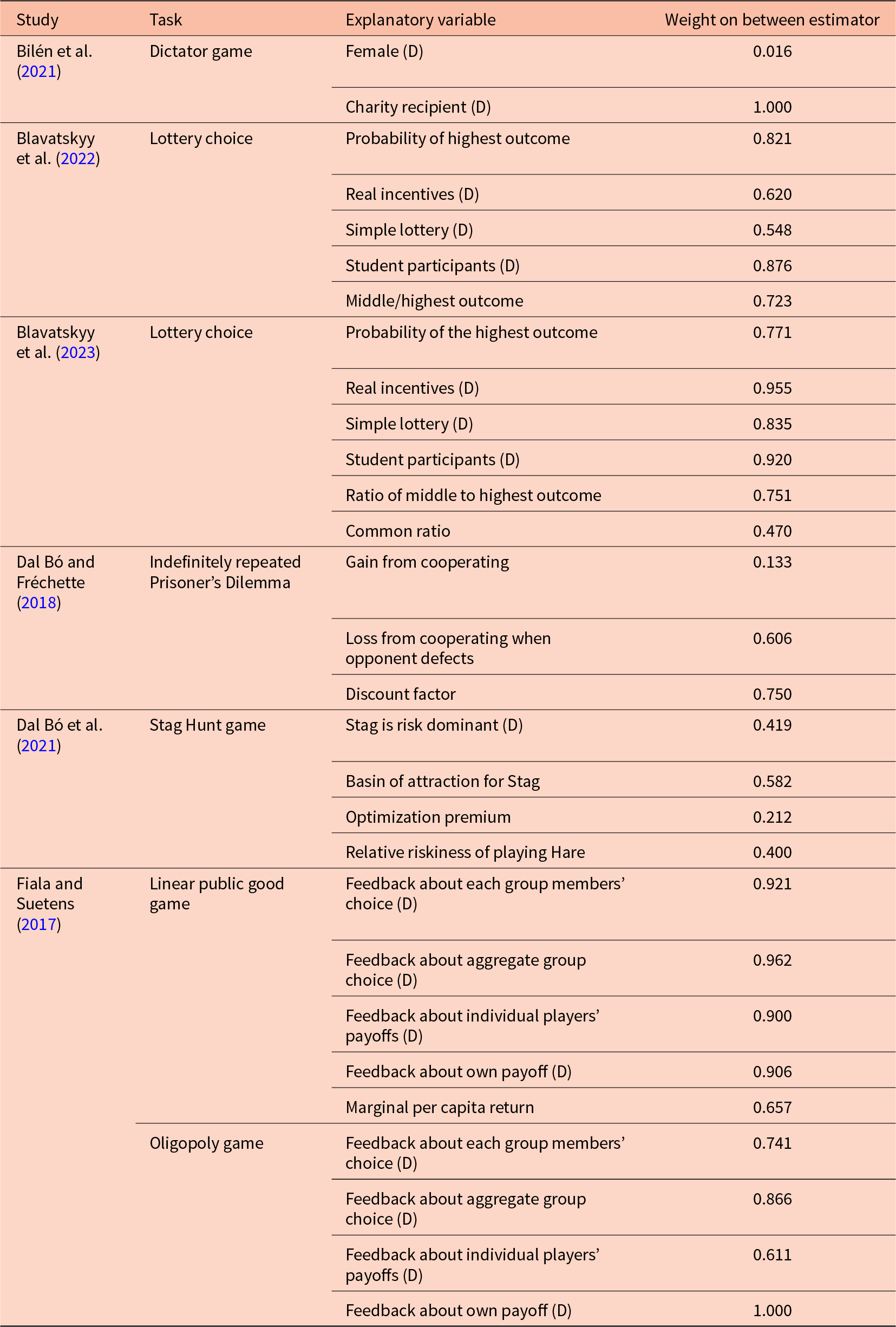
The first condition is something that we can check with our data. For example, Table 1 documents some studies that estimate pooled models from individual-level data.Footnote ⁴ The first column lists the study, the second column the topic of the study, the third column lists the explanatory variable (i.e.  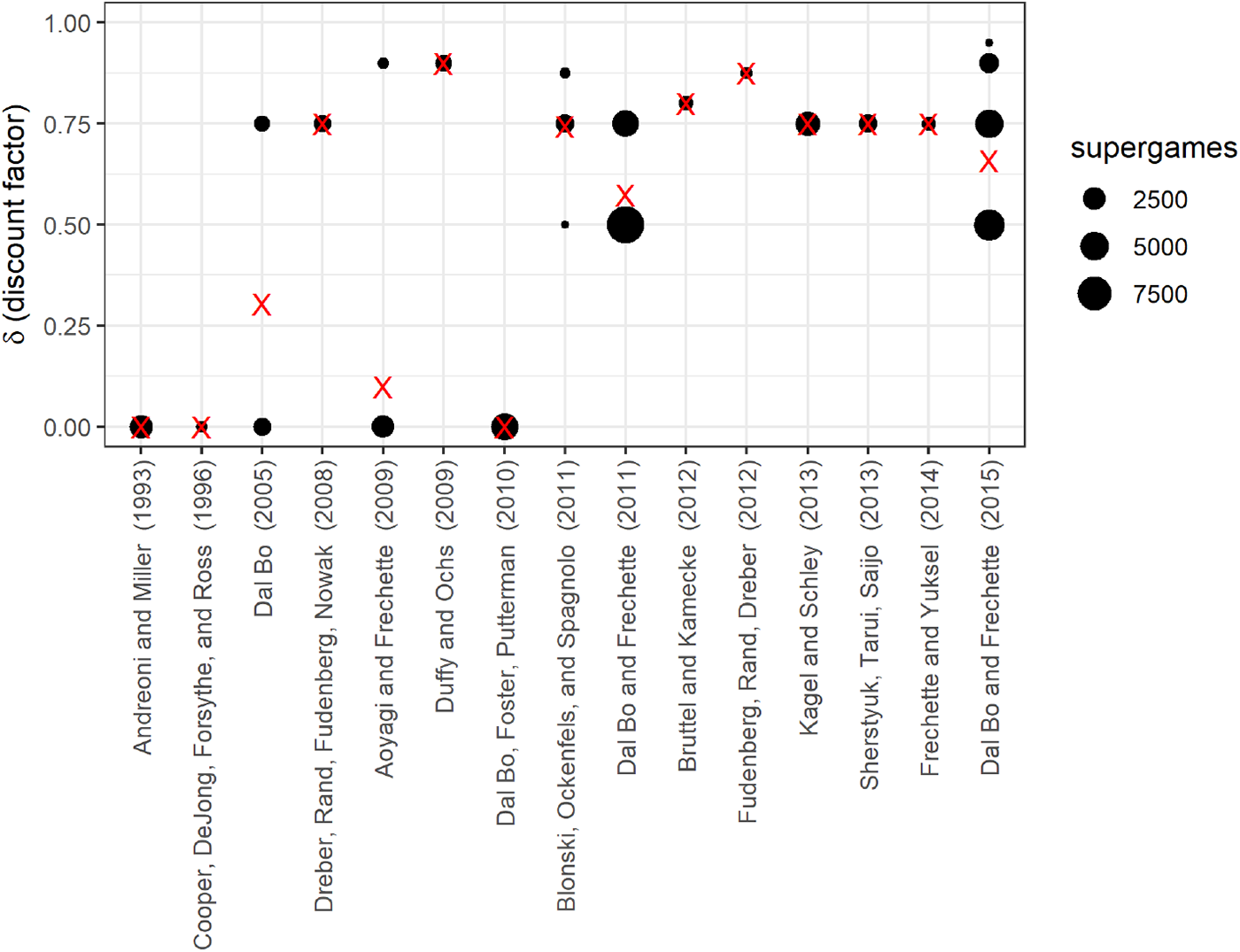$x_{e,i,t}$), and the rightmost column lists the weight placed on the between-experiments estimator $\tilde\beta_1$. If this weight is zero, then one does not need to worry about bias. However, none of these weights are zero, and furthermore most weights are closer to one than zero. Therefore, for typical uses of this technique, it is unlikely that we will be able to justify unbiasedness, or even just receiving a small weight, using this first condition. That the weight on the between-experiments estimator is substantial for most applications should in fact be unsurprising: it is uncommon for experiment conditions to be exactly replicated, and so average treatment conditions between experiments will likely be different. That is, when running a new experiment, an experimenter may replicate some or all of an existing study, but it is unlikely that they will only replicate an existing study. More likely, they will add extensions to the original design. Figure 1 takes a closer look at the data contributing to a 75% weight being placed on the between estimator for the effect of discount factor $\delta$ in the meta-study by Dal Bó and Fréchette (Reference Dal Bó and Fréchette2018). Each dot in this plot represents a unique discount factor studied in each experiment, and the red “X”s mark the within-experiment average treatment conditions (i.e.  $\bar x_e$). Clearly, average treatment conditions are not constant across experiments, as seen by the different heights of the red “X”s. Furthermore, this study includes some experiments with no variation in the discount factor. These experiments individually are unable to estimate the effect of discount factor on (say) cooperation, and so data from these experiments only inform the meta-study through the between-experiments estimator.

Table 1

Weight placed on the between estimator for various studies using pooled models. (D) indicates that the explanatory variable is a dummy variable. Weights are shown for the bivariate OLS estimator

Fig. 1

Discount factors used in the fifteen economic experiments on the indefinitely repeated Prisoner’s Dilemma examined in Dal Bó and Fréchette (Reference Dal Bó and Fréchette2018). Red “X”s mark the average treatment conditions

The second condition for unbiasedness, $\mathrm{cov}(\bar \epsilon_e,\bar x_e)=0$, requires that average errors in the experiment ( $\bar \epsilon_e$) are uncorrelated with average treatment conditions ( $\bar x_e$). This condition requires knowledge of the error terms in (2), and is therefore unverifiable. However, since experiments have different research questions for each new experiment, it is plausibly a problem. This exogeneity between experiments is also unlikely to hold in practice, as good experimenters will design their new experiments (i.e. choose their $x$s) based on their beliefs about how participants will respond to treatment conditions in their own laboratory. For example, suppose that we were designing a linear public goods game experiment, and we understood that participants in our subject pool were particularly uncooperative. We may choose to increase the marginal per-capita return above levels used in most past experiments if we need a good baseline level of cooperation. This would be choosing our $x$s in response to anticipated levels of $\epsilon$. Furthermore, good experimenters will use results of previous experiments, even if not from the same laboratory, in the design of new experiments. This, too, will induce correlation between average treatment conditions and the error term.Footnote ⁵

Correcting for this bias is possible using experiment-specific fixed effects. We would then place no weight on what can be learned from between-experiment treatment variation. Hence, if we believe that this kind of endogeneity is not present, we may not want to throw out this information.

Next, I use a Monte Carlo simulation to demonstrate the extent of the bias. Here, the true relationship between treatment variable $X$ and outcome variable $Y$ is:

\begin{equation*} Y_{e,i,t}=X_{e,i,t}+\eta_e+\epsilon_{e,i,t} \end{equation*}

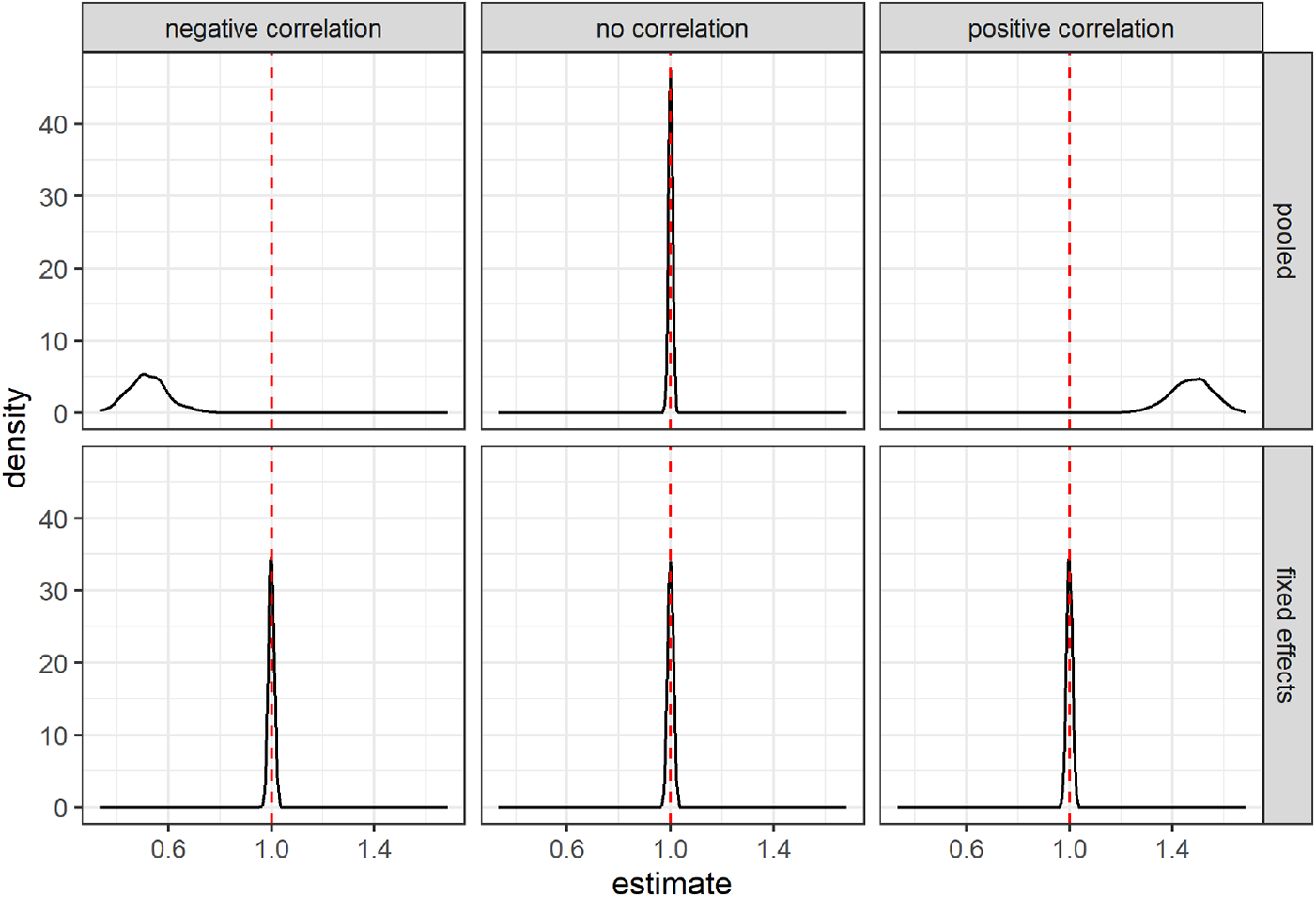
where $\eta_e$ is an experiment-specific effect, and $\epsilon_{e,i,t}$ is an idiosyncratic error term. I vary the way in which experimenters choose their treatment conditions in response to $\eta_e$. That is, $\eta_e$ is known to the experimenter but not the econometrician. I explore three different kinds of responses to this experiment-specific error term. Firstly, in the “no correlation” condition, experimenters do not take $\eta_e$ into account. Then, in the “negative correlation” condition, experimenters choose lower $X$ within their experiment as $\eta_e$ increases. Finally, in the “positive correlation” condition, experimenters choose larger $X$ within their experiment as $\eta_e$ increases. The simulation is set up so that approximately half the weight is placed on the between-experiments estimator for all conditions.Footnote ⁶ Figure 2 summarizes the results of the simulation by showing the kernel-smoothed density of the simulated slope estimates. The top panels present the results for the pooled estimator. Here we can see that when the experimenter does not choose $X$ in response to experiment-specific errors (middle panel), there is no problem with the pooled model. We can see that the distribution is centered on the true value of $\beta_1=1$. On the other hand, when there is a negative correlation between experiment-specific errors and $X$ (left panel), the pooled model is biased in the negative direction, and when there is a positive correlation between experiment-specific errors and $X$ (right panel), the pooled model over-estimates the treatment effect. The bottom panels show that including experiment fixed effects will eliminate this bias in both cases.

Fig. 2

Results of a simulation exploring various experimenter responses to experiment-specific error terms. The vertical red dashed line shows the true value of the estimand

Inspection of (2), the equation for $w_e$, shows that experiment-specific treatment effects receive a weight that is proportional to $\sum_{\forall i,t\in e}(x_{e,i,t}-\bar x_e)^2$. This is part, but not all, of the inverse variance for $\hat\beta_1^e$, assuming homoskedasticity within an experiment. Because of this, all else held equal, an experiment that (i) has more observations, and/or (ii) has more variation in the treatment variable will receive more weight. This is a desirable property of the weights, as experiments with these properties will, all else held equal, have more precise estimates of the treatment effect. On the other hand, absent from the weight is any estimate of the within-experiment variance of $\epsilon_{e,i,t}$. Hence, experiments with identical $x$s and the same number of decisions will receive identical weights, even if the treatment effect is estimated more precisely in one experiment compared to another. This means that $\hat\beta_1^\text{pooled}$ will be inefficient compared to more traditional methods of meta-analysis that take account of this precision. Furthermore, if it is appropriate to cluster standard errors when analyzing data within an experiment, this weighting will not take this into account. For example, suppose that for two experiments, it is appropriate to cluster standard errors at the participant level. Experiment $A$ has 10 participants making 100 decisions each, and experiment $B$ has 100 participants making 10 decisions each. $\hat\beta_1^\text{pooled}$ weights each of these experiments equally, even though experiment $B$ has more independent observations, and thus will most likely have a more precise estimate of the treatment effect.

3. Some remedies

The previous section shows that within-experiment randomization into treatments is not sufficient for the pooled OLS estimator $\hat\beta_1^\text{pooled}$ to be unbiased. The extent of this bias is a function of (i) the weight placed on the between-experiment estimator $\tilde\beta_1$, and (ii) the bias of $\tilde\beta_1$. While the weight on $\tilde\beta_1$ can be easily computed, its bias is a function of the experiment-average error terms $\{\bar \epsilon_e\}_{\forall e}$, and so one can only hypothesize about its bias. While drawing conclusions from $\hat\beta_1^\text{pooled}$ may be worthwhile if we can establish that this bias (through reasoning) and/or weight (through computation) is small for our particular application, there will be other applications in which we need to be wary. The remainder of this section first outlines how this bias term can be completely eliminated by ignoring all studies that do not have any variation in $x_{e,i,t}$, and then how the remaining within-experiment estimators can be combined more efficiently.

If we are unconvinced that the between-experiment estimator $\tilde\beta_1$ is unbiased, then constructing an estimator that places no weight on this component will solve the bias problem. Including experiment fixed effects in the regression will ensure that weight will only be placed on the unbiased within-experiment estimators $\hat\beta^e$. This is equivalent to simply dropping all of the experiments with no variation in $x_{e,i,t}$ from the analysis. Table 2 of Cooper and Dutcher (Reference Cooper and Dutcher2011) and Table 2 of Alm and Malézieux (Reference Alm and Malézieux2021) are examples of using fixed effects, and so the estimators used in these Tables do not suffer from this source of bias. Importantly, if present, the bias of $\tilde\beta_1$ is not remedied by experiment random effects, or other multi-level or hierarchical models. These models assume that the random effects are uncorrelated with $x_{e,i,t}$, which would not be true if $\tilde\beta_1$ is biased. That is, the random effects model assumes that the group-specific random effects are uncorrelated with the explanatory variable. When experimenters choose their treatment conditions in response to the error term, this condition is not satisfied, and the slope estimator is biased.

Table 2

Decomposition of the pooled estimator in Fiala and Suetens (Reference Fiala and Suetens2017), estimating the effect of having feedback about each group member’s contribution in a public goods game on average group contributions. Standard errors for weighted estimates are clustered at the experiment level. Standard errors for estimates within experiments are heteroskedasticity-robust

Suppose now that we are analyzing just experiments with some variation in the treatment variable, and so any weighting (that adds to one) of the remaining within-experiment estimators will be unbiased. The goal could therefore be to weight the estimators in a way that minimizes the variance:

\begin{equation*} V\left(\hat\beta_1\right)=\sum_{\forall e}w_e^2 V\left(\hat\beta_1^e\right) \end{equation*}

Choosing weights that are proportional to the inverse of the variance of the within-experiment estimator minimizes this variance. That is:

\begin{equation*} w_e= \frac{V\left(\hat\beta_1^e\right)^{-1}}{\sum_{\forall e}V\left(\hat\beta_1^e\right)^{-1}} \end{equation*}

In practice, we replace the unknown quantity $V\left(\hat\beta_1^e\right)$ with its estimate, which is the squared standard error of $\hat\beta_1^e$. Examples of this weighting estimator being used for economic experiments can be found in Ioannidis et al. (Reference Ioannidis, Offerman and Sloof2020) (see discussion around their Table 3) and De Quidt et al. (Reference De Quidt, Fallucchi, Kölle, Nosenzo and Quercia2017) (see their footnote 15). Note that while clustered standard errors at the experiment level may be appropriate to more accurately express the uncertainty we have in our pooled estimate, they will not affect the weighting, and so will have no bearing on the point estimate.

Table 3

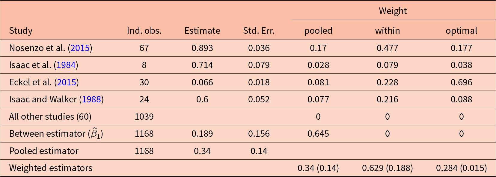
Decomposition of the pooled estimator in Fiala and Suetens (Reference Fiala and Suetens2017), estimating the effect of the marginal per capita return in a public goods game on average group contributions. Standard errors for weighted estimates are clustered at the experiment level. Standard errors for estimates within experiments are heteroskedasticity-robust

In summary, these results motivate the following advice for practitioners who are performing a meta-analysis with decision-level data:

1. (1) Be aware of how many experiments in your dataset can individually estimate the desired treatment effect. These are the experiments that vary the treatment variable.

2. (2) One can always calculate the weight placed on the between-experiments estimator (and the between-experiments estimate itself). If this weight is large, it is an indicator that the potentially biased between-experiment estimator is driving the results.

3. (3) Consider estimators that are robust to this source of bias. If you want to use OLS, at least include experiment fixed effects. Otherwise, consider aggregating experiment-specific estimates using either an inverse variance-weighted estimator or the Rubin (Reference Rubin1981) model.

4. (4) Understand why the experiments were designed the way they were. Be aware of situations where experimenters would want to adjust their treatment conditions in response to expectations about the error term.

5. (5) If you have a few experiments in the dataset, consider reporting the pooled estimates alongside the fixed effects estimates and discussing the limitations of drawing conclusions from the pooled estimates.

4. Examples

4.1. Fiala and Suetens (Reference Fiala and Suetens2017)

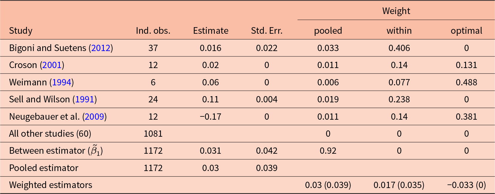
Fiala and Suetens (Reference Fiala and Suetens2017) uses data from linear public good and oligopoly game experiments to investigate the influence of different kinds of feedback on participants’ choices. In this example, I analyze their data on the public good games to answer two research questions. Firstly, I estimate the effect of having or not having feedback about each group member’s choice provided. As shown in Table 1, the pooled OLS estimator places about 92% of its weight on the between-experiments estimator here. Secondly, I investigate the effect of the marginal per capita return (MPCR) on participants’ choices. Here, Table 1 shows that the pooled OLS estimator places about 66% of its weight on the between-experiment estimator for this effect. In order to be comparable to the original analysis of Fiala and Suetens (Reference Fiala and Suetens2017), I treat groups of participants as the level of independent observation.

Table 2 decomposes the pooled estimator used in Table 4, column 1 of Fiala and Suetens (Reference Fiala and Suetens2017) to estimate the effect of feedback about individual group choices on average group contributions. While the dataset includes 65 studies in total, only five of these varied in this kind of feedback. That is, these experiments only contribute to the pooled estimator through the between-experiments estimator. As such, only 8% of the weight of the pooled estimator goes to the within-experiment estimates, which are itemized by study in the top panel of Table 2. Importantly here, the between-experiment estimate ( $\tilde\beta_1$) is larger than all of the within-experiment estimates. If what we learn about feedback from between-experiment variation is biased, the pooled estimator is placing a lot of weight on this estimator. This variation largely comes from the remaining 33 studies that never provide this feedback, and 27 that always provide this feedback.Footnote ⁷

Table 4

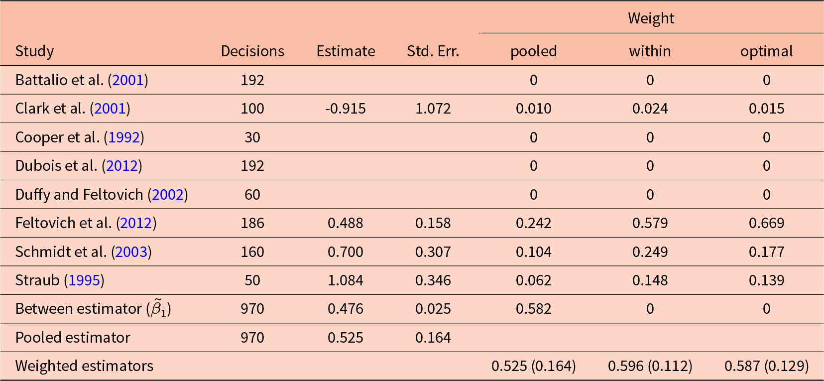
Decomposition of the pooled OLS estimator for Dal Bó et al. (Reference Dal Bó, Fréchette and Kim2021). Each estimate is for the effect of the basin of attraction of Stag on the probability of choosing Stag in a Stag Hunt game. Missing estimates indicate that the within-experiment estimator is undefined for these experiments. This is because there is no variation in the treatment variable within these experiments

Table 3 does a similar decomposition for the marginal per capita return.Footnote ⁸ For this explanatory variable, 65% of the weight is placed on the between estimator $\tilde\beta_1$. Perhaps most striking in this decomposition is that the within (fixed effects) estimate (0.629) is almost double that of the pooled estimate (0.340). This is because the between estimate is much smaller than most of the within-experiment estimates, and receives a substantial fraction of the weight. Furthermore, the optimally-weighted estimator (rightmost column) weights the within-experiment estimates very differently from the within estimator (second column from the right), with the latter placing almost half the weight on Nosenzo et al. (Reference Nosenzo, Quercia and Sefton2015), and the former placing almost 70% of the weight on Eckel et al. (Reference Eckel, Harwell and Castillo2015). This highlights the difference between the pooled and within weights, which do not fully take into account the precision of the within-experiment estimators, and the optimally-weighted estimator, which explicitly weights according to this precision.

In summary, for both of these outcome variables, the potentially biased between-experiments estimator receives the majority of the weight. This is because only a handful of studies actually vary the treatment variable of interest.

5. Conclusion

When combining decision-level data from more than one economic experiment, the pooled OLS estimator can be written as a weighted sum of the within-experiment estimators for the treatment effect and the between-experiment estimator for the treatment effect. An immediate consequence of this is that all of these estimators must be unbiased for the pooled estimator to be unbiased. Typical experimental designs will take care of this for the within-experiment estimators, however more care may be needed with the between-experiment estimator. For this to be unbiased, we need the average treatment variable for an experiment is uncorrelated with the average error term in an experiment. This condition may not hold if experimenters choose their average treatment variable in response to their beliefs about choices in the experiment. In the examples shown in the previous section, these between-experiment estimators received the majority of the weight.

Furthermore, conclusions drawn from the pooled estimator may be overstating what we have learned from the experiments included in the study. This is because some weight, and in practice a substantial weight, is placed on the between-experiment estimator. Ideally, we would like to learn about treatment effects through exogenous variation of the treatment variable. Many studies included in these pooled analyses do not have this variation for some explanatory variables. This calls for a more careful consideration of what studies are included, and not included, in a meta-analysis. In particular, if an experiment cannot individually provide an answer to the research question, then its contribution to the meta-study will be solely through between-experiment variation. This means that there may need to be more experiments run to estimate the same treatment effect before we can meaningfully combine them in a meta-analysis. On the other hand, Meager (Reference Meager2019) meaningfully aggregates the results of just seven experiments, so this number need not be too high.

It should be noted that whether we are using pooled OLS, instrumental variables, or an inverse variance-weighted estimator, all of these estimators are weighted averages of experiment-specific estimates (and in the case of pooled OLS, the biased between-experiments estimate as well). While the latter two are unbiasedly aggregating treatment effect estimates, they are not necessarily estimating an “average treatment effect”. An alternative estimator that aims to estimate this average treatment effect is the Rubin (Reference Rubin1981) model, which explicitly models between-experiment variation of treatment effects. See Meager (Reference Meager2019) and for an application of this technique to field experiments, Bland (Reference Bland2025) for an application related to laboratory experiments.

The result that a pooled estimator can be written as a weighted average of within estimators and a between estimator is not new. However, this paper contributes to the experimental economics literature by putting this result into the context of meta-analysis using decision-level data.

This paper also stresses the importance of understanding why there is between-experiment variation in average treatment conditions in a meta-study. If this variation is due to experimenters endogenously choosing their treatment conditions in response to expected behavior, then we should worry about the conclusions drawn from the pooled OLS model. In this case, other methods, such as using fixed effects, should be preferable. On the other hand, if we understand that differences across experiments are not due to experimenters choosing these things, then we need not worry about this bias.

While the remedies discussed here address the bias associated with experimenters choosing their own treatment conditions, they do not address other, perhaps more worrying, sources of bias potentially present in meta-analyses. For example, publication bias (e.g. Ioannidis et al. (Reference Ioannidis, Stanley and Doucouliagos2017)) is a form of selection bias. If this source of bias is also present, then dropping all studies that do not individually answer the research question of the meta-study will not fully eliminate bias in the aggregated treatment effect. As such, the fixed effects or optimal weighting approaches discussed here are not magic bullets and need to be applied with the understanding that publication bias may still be present.

In practice, adding an experiment to a meta-study that cannot individually estimate a treatment effect comes with a trade-off. On the one hand, if the experiment-average errors are correlated with average treatment variables, then we will introduce bias to our pooled estimator. On the other hand, there is objectively less information to learn from if we ignore such a study. Where there are few experiments available with variation in the explanatory variable of interest, reporting both the pooled OLS estimator and the weighted within-experiment estimator is perhaps advisable. In doing this, we report both a (potentially biased) “big picture” view of how the variables in our data are related, and then also focus in on what we can learn from the experiments that can individually answer our research question.