





1. Introduction
The predominantly ice-covered continent of Antarctica is the single largest component of the global cryosphere. One of the key parameters governing its radiative energy budget is surface albedo, defined as the fraction of incoming solar (shortwave) radiation reflected away from the surface. Scattering of solar radiation occurs when the refractive index of the medium changes. Thus, the broadband albedo of a snowpack is primarily determined by the number of ice–air interfaces in a unit volume of snow at the depths where solar radiation can penetrate, with near-surface layers contributing more to the overall reflection. Classically, snow grain size was used as the parameter to describe this dependence (Wiscombe and Warren, Reference Wiscombe and Warren1980), but difficulties in establishing universally applicable relationships between physical and optically equivalent grain sizes (and their distributions within the optically active snowpack) have led to parameters such as specific surface area (SSA) of snow becoming commonplace replacements (Gallet and others, Reference Gallet, Domine, Zender and Picard2009; Gardner and Sharp, Reference Gardner and Sharp2010).
Illumination geometry also affects snow albedo. This is intuitively clear, as radiation entering the snowpack from a shallow angle of incidence travels longer in the near-surface snow layers and thus has more chances of escaping the snowpack via scattering. To account for this effect, solar zenith angle (SZA) is typically incorporated in snow albedo modeling. While Antarctic snowpacks of the continent’s interior are typically cold and nonmelting, seasonal snowmelt does occur on the ice shelves and nearby coastal areas of the ice sheet (Mousavi and others, Reference Mousavi, Colliander, Miller and Kimball2022). Melting snow exhibits rapid diurnal changes in the optical properties, causing nonsymmetric variation in snow albedo relative to local noon (Wiscombe and Warren, Reference Wiscombe and Warren1980) that requires more complex treatments to model (Manninen and others, Reference Manninen, Jääskeläinen and Riihelä2020). The optical properties of the atmosphere, particularly through the presence and optical thickness of clouds, also play a key role in the determination of (blue-sky, i.e., under natural illumination) surface albedo of snow. Clouds alter the effective SZA of incident solar radiation and change its spectral composition, with the outcome typically being an increase in snow albedo under cloudy skies (Warren, Reference Warren1982; Gardner and Sharp, Reference Gardner and Sharp2010). Finally, impurities in the optically active snow layers absorb solar radiation and effectively lower the snow albedo (Warren and Wiscombe, Reference Warren and Wiscombe1980), with additional snowmelt implications which could be substantial if the impurity loading is sufficiently large (Dumont and others, Reference Dumont, Brun, Picard, Michou, Libois and Petit2014). However, Antarctic snow is generally pure (Grenfell and others, Reference Grenfell, Warren and Mullen1994) as the remoteness and lack of human habitation shield the snow cover from local or remotely transported impurities, except in the vicinities of research stations (Casey and others, Reference Casey, Kaspari, Skiles, Kreutz and Handley2017).
Apart from these factors, it has long been recognized that surface roughness (SR) also impacts both directional snow reflectances, with implications for remote-sensing instruments, and snow albedo (Warren, Reference Warren1982; Hudson and others, Reference Hudson, Warren, Brandt, Grenfell and Six2006). Both macroscopic surface features such as sastrugi and the millimeter-/centimeter-scale irregularities of the snow surface are relevant (e.g., Leroux and Fily, Reference Leroux and Fily1998; Warren and others, Reference Warren, Brandt and O’Rawe Hinton1998; Zhuravleva and Kokhanovsky, Reference Zhuravleva and Kokhanovsky2011; Manninen and others, Reference Manninen2021), meaning that SR effects manifest at multiple scales. Regardless of scale, SR alters the incidence angle distribution of incoming solar radiation and increases multiple scattering from facet-to-facet scattering events (Warren and others, Reference Warren, Brandt and O’Rawe Hinton1998). However, these effects on albedo also depend on wavelength. In the visible wavelengths, the absorption coefficient of ice is so low that photons have a high chance of surviving even multiple scattering events in the surface layer of a rough snowpack (Wiscombe and Warren, Reference Wiscombe and Warren1980). Conversely, at higher wavelengths where ice becomes more absorbing, photons trapped in surface cavities are quickly absorbed during scattering events, increasing the relative importance of SR effects in the near-infrared regime and beyond (e.g., Larue and others, Reference Larue2020). The size of the roughness features present also has an influence, which is connected to the illumination geometry; for example, the penitente features present in mountain glaciers may reach heights of more than a meter, causing substantial surface albedo changes even at high solar elevation (Lhermitte and others, Reference Lhermitte, Abermann and Kinnard2014).
Quantification of snow SR and its albedo impact has been challenging. Photography of graded plates inserted into the snowpack has been the earliest and most widely used method (e.g., Rott, Reference Rott1984; Williams and others, Reference D, G, E and V1988; Löwe and others, Reference Löwe, Egli, Bartlett, Guala and Manes2007; Manninen and others, Reference Manninen, Anttila, Karjalainen and Lahtinen2012; Anttila and others, Reference Anttila, Manninen, Karjalainen, Lahtinen, Riihelä and Siljamo2014), although limited in the spatial sampling scale and in only capturing roughness variability in one direction along the plate profile. With the advent of field-transportable laser scanners, terrestrial laser scanner observations of the snow surface have begun to supplement and even replace the older methods (Kukko and others, Reference Kukko, Anttila, Manninen, Kaartinen and Kaasalainen2013; Lacroix and others, Reference Lacroix2008), as they offer a combination of potentially large spatial coverage combined with the high-density sampling of laser point clouds.
The advances in observation capability have fueled new modeling efforts into the albedo effects of snow SR. Larue and others (Reference Larue2020) and Manninen and others (Reference Manninen2021) investigated the albedo effects on alpine and seasonal (boreal) snow, respectively, through a combination of in situ observations and modeling. Both studies found similar snow albedo decreases from SR (typically on the order of 0.01–0.05), which depend on the solar illumination geometry and on the overall reflectivity of the snowpack. Other efforts have focused on applying airborne observations of snow directional reflectance (Gatebe and King, Reference Gatebe and King2016) to produce a surface reflectance correction for macroscopic roughness features of Arctic snow (Lyapustin and others, Reference Lyapustin2010).
The SR feature distributions vary between the polar regions. Seasonal snowpacks, such as those studied by Larue and others (Reference Larue2020) and Manninen and others (Reference Manninen2021), are characterized more by small-scale roughness than macroscopic features, although, e.g., suncups occur during melt. Larger SR features over both polar regions form under wind-driven movement, and a thorough review of the features and their formation mechanisms is presented in Filhol and Sturm (Reference Filhol and Sturm2015). The study of Warren and others (Reference Warren, Brandt and O’Rawe Hinton1998) pioneered the quantification of sastrugi-scale effects on the Antarctic ice-sheet albedo, and SR of Arctic snow at small scales was measured by Lacroix and others (Reference Lacroix2008), but to our knowledge, a similar small-scale effect investigation has not been undertaken for Antarctic snow. Our aim is to address this gap.
Therefore, here we report on a field campaign in the region of Dronning Maud Land (Queen Maud Land) in Antarctica during the austral summer of 2022–23, designed to investigate the millimeter-to-centimeter SR of Antarctic snow and its relationship to the observable snow properties and snow albedo. The centerpiece of our research is the use of an unmanned aerial vehicle (UAV)-mounted laser scanner in combination with concurrent observations of snow broadband albedo and relevant physical and optical properties of the snowpack. This approach enables us to map SR over larger areas than with terrestrial sensors. Alongside the albedo investigation, the second goal of the field campaign was to ascertain and quantify the effects of SR on spaceborne altimeter observations over the field sites. However, this inquiry will not be reported here but in a separate future study.
The goals of this study are threefold: first, to report the observed spatiotemporal variability of both surface albedo and SR of the study area in western Queen Maud Land; second, to construct model-based surface albedo estimates for smooth snow surfaces based on our observed snow radiative properties; and third, to apply the SR model of Manninen and others (Reference Manninen2021) to these data to ascertain if it improves their agreement given the uncertainties of the measurements and analyses. While noting the importance of macroscale SR features and the wavelength dependency, our focus in this study is on the impact on broadband snow albedo at the millimeter-to-centimeter scales and in the resolution range of the laser scanner observations.
2. Methods and data
We begin with a brief overview of the LAS3R campaign at Aboa research station, noting that the full details are available in Leppänen and others (Reference Leppänen, Kukko, Rimali, Riihelä and Tisler2025). We then describe the relevant specific measurements and algorithms in detail in the following sections by measurement type. Finally, we describe the snow albedo parameterization and SR model used in this study.
2.1. Overview of LAS3R campaign at Aboa research station, Queen Maud Land, Antarctica
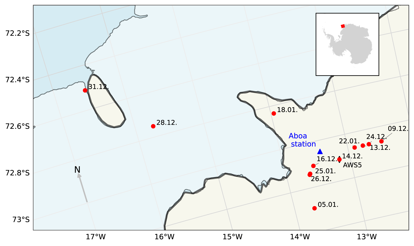
The LAS3R field campaign took place in the region surrounding the Finnish Antarctic research station Aboa during the austral summer of 2022–23 (Fig. 1). Applicable field observations were collected between 19 November 2022 and 25 January 2023. The field site locations and measurement timings were designed to collocate with overpasses of the ICESat-2 and CryoSat-2 satellites, as the study of SR effects on altimetry measurements was another major motivator for the LAS3R project and campaign.
Locations and dates of visit at LAS3R measurement sites in Queen Maud Land, Antarctica. Aboa station is marked with a blue triangle, and AWS5 site is marked with a black diamond. AWS5 was visited periodically (see Table 1 for the dates). Thick black line indicates the grounding line, and the thin gray line indicates ice-shelf edge, separating open ocean (blue) from the ice shelf (light blue). Grounding line and ice-shelf edge from the SCAR Antarctic Digital Database, 2024.

Figure 1 Long description
A map of Queen Maud Land, Antarctica, displays various locations and dates. Aboa station is marked with a blue triangle. The AWS5 site is indicated near several red dots, each labeled with dates: 09.12, 13.12, 14.12, 16.12, 22.01, 24.12, 25.01 and 26.12. Additional red dots with dates are scattered across the map: 31.12, 28.12, 18.01 and 05.01. The map includes latitude and longitude lines, with a small inset map showing the region's location in Antarctica. A north arrow is present for orientation.
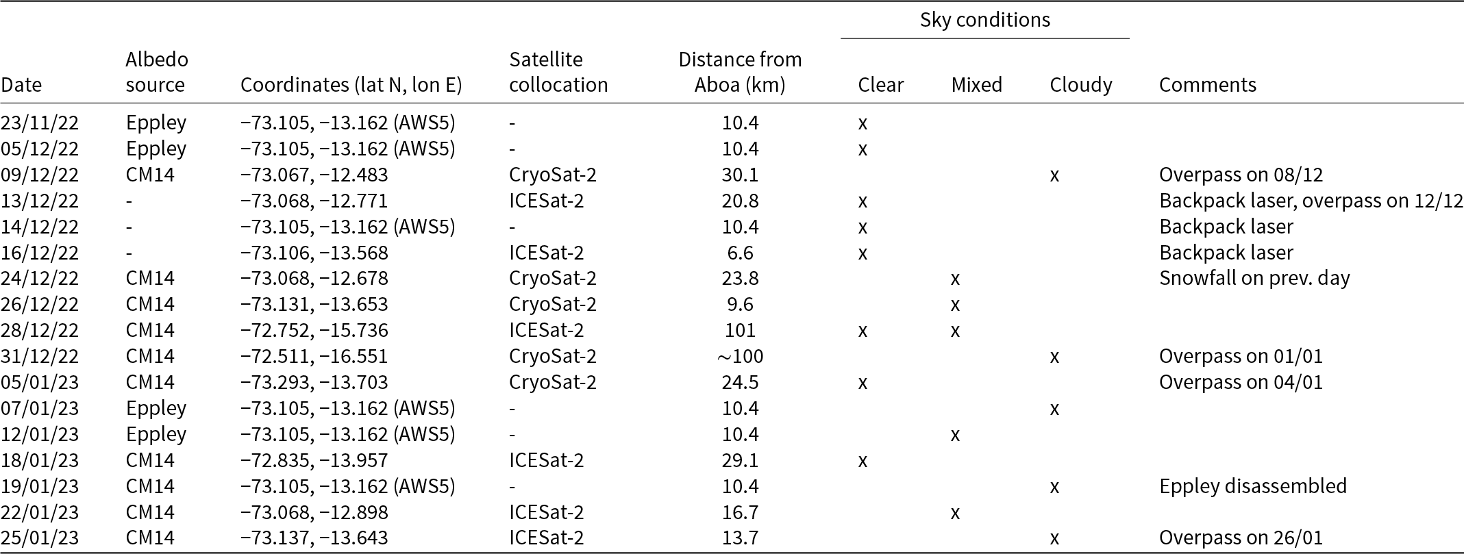
During the first half of the campaign, adverse weather and initial technical issues limited data availability. A storm interrupted all observations between 25 November and 3 December. Technical issues further prompted a switch to using the backpack-mounted laser scanner between 13 and 16 December. In total, 11 field sites were visited, along with recurring observations near the AWS5 automatic weather station during 4 days, to monitor temporal variability in albedo and SR at a fixed site (AWS5 visited on 6 days, but no UAV laser scanner data were available on 14 December and no albedo observations were available on 19 January). Observation days with a complete observation set are listed in Table 1, and they form the core dataset applied in this study; continuous albedo observations from the Eppley albedometer installed near AWS5 are additionally presented outside these dates for a more detailed view into the development of the optical properties and surface albedo during the full campaign period. Weather conditions during the latter half of the campaign were generally favorable. Snowfall at the field site was observed by the crew on 23–24 December.
Observation dates and parameters of data used in this study, a subset of all LAS3R measurements.

Table 1 Long description
This table presents data from LAS3R measurements, detailing observation dates, albedo sources, geographic coordinates, satellite collocations, distances from Aboa, sky conditions, and comments. Key data points include frequent use of CM14 and Eppley albedo sources, with coordinates mostly around AWS5. Satellite collocations with CryoSat-2 and ICESat-2 are noted, with distances from Aboa ranging from 6.6 km to approximately 100 km. Sky conditions vary, with clear, mixed, and cloudy conditions recorded. Notable events include satellite overpasses and weather occurrences like snowfall. The data suggests a focus on specific geographic locations and satellite interactions, with varying sky conditions potentially impacting measurements.
The measurements followed a similar protocol at each site. The laser scanner drone, Avartek Boxer, flew a grid pattern over the area covering the albedo measurement site and surroundings; daily coverage ranged ∼1 km2. At AWS, the grid was 500 m × 500 m. A set of snow pits (one to six per day) was sampled in the area for vertical profiles of snow temperature, density and specific surface area (SSA). The drone carrying the CM11 pyranometer flew over the area in a pattern roughly matching that of the laser scanner drone. Finally, a lightweight camera DJI Mavic 2 Pro drone captured red–green–blue (RGB) imagery of the area to construct a top view mosaic of the surface appearance. The mosaics were used to create area bounds for SR computation and to visually verify the resulting SR features against collocated features in the mosaics. We next describe these measurements and their data processing.
2.2. Albedo measurements
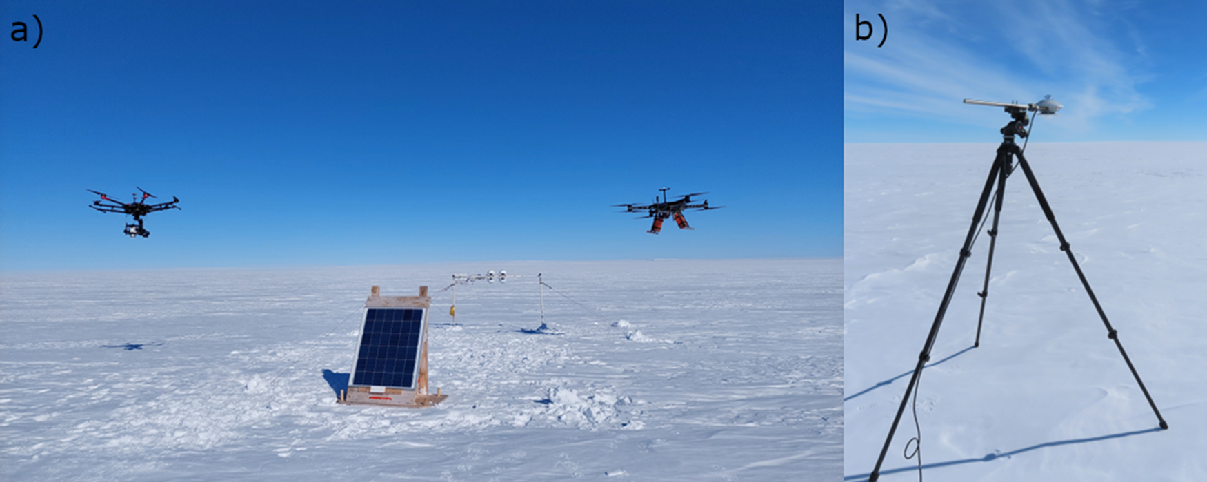
We measured surface albedo during the campaign with two approaches. On the ground, a fixed Eppley radiation station measured albedo continuously throughout the campaign in the vicinity of the AWS5 weather station. To amend the spatial coverage, we further used a lightweight, tripod-mounted CM14 albedometer at the various field sites (Table 1) during the drone and snow pit observations. In the air, a drone-mounted and gimbal-stabilized CM11 provided reflected shortwave flux measurements to be combined with the ground-measured irradiance for an albedo measurement with broader spatial coverage. Figure 2 shows the instruments in their operational configurations in the field. The details of the instruments are described in the following subsections.
In panel (a), on the left, the DJI drone carries the downward-pointing and gimbal-stabilized CM11 pyranometer. In the middle, the Eppley radiation station and its solar panel. On the right, the Avartek drone carries the Riegl VUX-120 laser scanner. In panel (b), the CM14 albedometer is mounted on a tripod in measurement configuration.

Figure 2 Long description
Panel a) displays a snowy landscape with two drones flying above. One drone is on the left and the other is on the right. In the center, there is a solar panel mounted on a wooden frame. The area is covered with snow and the sky is clear. Panel b) shows a tripod-mounted device on a snowy surface. The tripod is positioned centrally and the sky is visible in the background, indicating a clear day.
2.2.1. Eppley and CM14
The Eppley radiation station was installed at the AWS5 site. The radiation station has two broadband upward- and two downward-pointing sensors, one each for short- and longwave wavelengths. The instrument has two legs, and sensors are installed to a bar between them. Installation was made so that the shades were minimized at noon. The height of the sensors was ∼120–140 cm above the snow surface, depending on the transient presence of new snow and drifted snow below the instrument. The uncertainty analysis of the albedo measurements is described in Pirazzini and others (Reference Pirazzini, Vihma, Granskog and Cheng2006), as the same sensor and measurement setup is used here. Briefly, the albedo measurement uncertainty is estimated at 5% for clear-sky and 1–4% for cloudy sky situations (at coverage factor k = 1, i.e., 68% of observation errors fall in this range).
The Kipp & Zonen CM14 albedometer is a back-to-back configuration of two CM11 pyranometers, which measure the incident and reflected shortwave broadband (310–2500 nm) radiative fluxes. In our measurement configuration, the albedometer was installed on a short boom and mounted on a camera tripod. As the tripod legs block a fraction of the reflected flux, a correction is applied to that data as described in Manninen and others (Reference Manninen2021), amounting to a reflected flux increase of 7% after verification with the drone-mounted CM11 observations described in the next section. The albedometer was calibrated against a reference pyranometer at the Finnish Meteorological Institute prior to the campaign and monitored during operation periods to guard against riming of the pyranometer domes, as the instrument is not ventilated. The total measurement uncertainty of the albedometer is assessed to be 5% after the corrections (reported conservatively at k = 1, as, e.g., instrument leveling is variably imperfect in field conditions).
All albedo observation data from periods when SZA > 70° were discarded to avoid additional errors related to the imperfect cosine responses at low Sun elevation conditions (Michalsky and others, Reference Michalsky, Harrison and Berkheiser III1995). Also, all data with unphysical measured albedo (<0 or >1) were discarded.
The increase in snow albedo under cloudy skies is well known (Warren and Wiscombe, Reference Warren and Wiscombe1980), but neither Eppley nor CM14 features separate measurements of incoming direct and diffuse irradiance. To obtain a general classification of the data into clear and cloudy sky observations, we adopted a simple processing scheme where each irradiance measurement was compared to a simulated clear-sky irradiance from the pvlib library following Bird and Hulstrom (Reference E and Hulstrom1981). If the difference was less than 100 W m−2, the measurement was considered clear sky. For the clear-sky simulation, we applied climatologically appropriate (constant) aerosol optical depth of 0.03 at 380 and 500 nm, a precipitable water column of 0.07 cm, ozone column of 0.2 cm, an ambient pressure of 93 100 Pa and exoatmospheric irradiance of 1364 W m−2 with an asymmetry factor of 0.7. The air mass was based on the SZA of each measurement, and the surface albedo in the calculation was that of each ground-based measurement. The binary classification of clear/nonclear sky is then simply averaged over each measurement day to obtain daily clear-sky fractions corresponding to the periods of measurement for Eppley and CM14. We acknowledge that this classification is quite basic, but our testing (see Section 3) proved it capable of producing a delineation of cloudy and clear scenes, which conformed with observed albedo variations at the diurnal and daily mean levels.
2.2.2. Drone-mounted CM11 combined with ground-based irradiance
The Kipp & Zonen CM11 pyranometer was mounted alongside the Rikola hyperspectral camera on a custom three-dimensional (3-D)-printed frame. This downward-facing payload was stabilized using a Gremsy H16 gimbal, installed on a DJI Matrice 600 Pro drone to ensure steady measurements during flight. The pyranometer generates analog signals in microvolts based on the detected radiance. These signals are converted to digital format using an analog-to-digital module and processed with custom Python code running on a Raspberry Pi computer. Additionally, the code retrieves time and location data from a Global Navigation Satellite System (GNSS) receiver connected to the computer.
The reflected solar flux observations from the drone-mounted CM11 are combined with incoming solar flux data from either the Eppley or CM14 albedometer to form the airborne estimate of surface albedo over the measurement sites. We acknowledge that the combination is expected to produce realistic estimates only under completely clear or completely cloudy skies, when the incoming solar flux consists of either predominantly direct or diffuse irradiance and is thus sufficiently homogeneous across the drone’s flight path (Levy and others, Reference Levy, Burakowski and Richardson2018). Because of these limitations, we apply the UAV-derived albedo estimates only toward a similarity assessment with the ground-based measurements from both Eppley and CM14. The measurement uncertainty is not well-known but likely cannot exceed the ground-based measurements due to the residual in-flight instabilities even with gimbal stabilization, as well as the need to have fully equal irradiance fields over both the ground sensor and the drone. We thus consider a 5% measurement uncertainty as the best-case scenario for this setup, valid for low-wind, clear-sky situations.
2.3. Snow pit-derived snow optical parameters from IceCube
Vertical specific surface area (SSA) profiles were measured with an IceCube instrument (manufactured by A2 Photonic Sensors) from the snow pits excavated at each field site. SSA is a widely used parameter to express the optical properties of ice grains, and its estimation from spectroscopic measurements is less prone to operator subjectivity than the estimation of snow grain size distributions from, e.g., graded plate photography (Gallet and others, Reference Gallet, Domine, Zender and Picard2009). The IceCube SSA measurement is based on the reflectance of a 1310-nm infrared laser from a snow sample surface. The measurement principle and snow sampling process of the IceCube are described in more detail in Leppänen and others (Reference Leppänen, Kontu, Hannula, Sjöblom and Pulliainen2016), and the associated error analysis is presented in Leppänen (Reference Leppänen2024).
For each field site, one to six snow pits were sampled, including vertical profiles of snow temperature and density. The vertical profiles typically extended to depths of 25–30 cm, as the primary interest was in the snow properties of the optically active layers. Vertical sampling density varied by observed layering; typically, SSA was sampled at every 2 cm intervals, but for thick (>5 cm) layers, the sampling was done at every 5 cm intervals. The daily mean SSA of the topmost 6 cm of snow samples was considered to represent the snowpack SSA for albedo determination in this study.
2.4. Laser scanner observations of snow SR
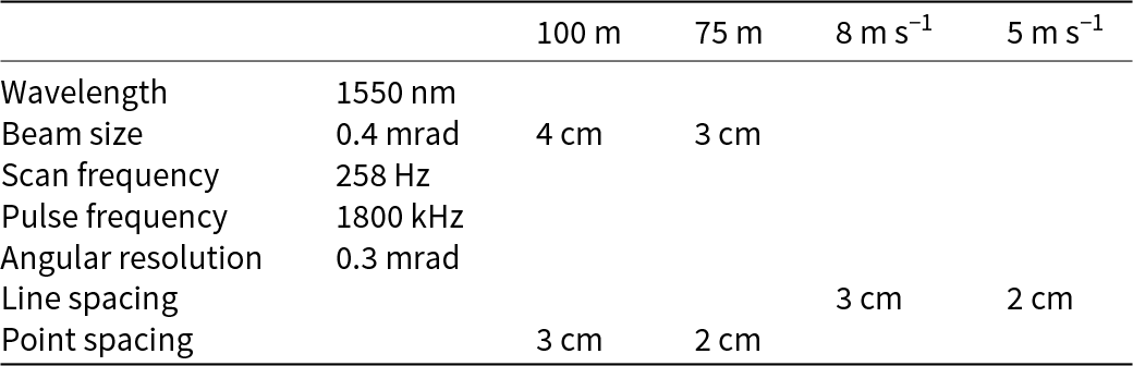
The snow SR was sampled by high-resolution UAV laser scanning, which provides microtopographic observations over large areas. In the study, we typically flew 600 m × 1600 m survey grids, with coincident flight altitude and flight line spacing (100 m/100 m and 75 m/75 m), implying 100% side overlap. The more specific scanning parameters are summarized in Table 2, showing that the resulting 3-D point clouds reconstructing the surface below have 2 and 3 cm sample spacing in both along- and cross-track directions with 75 and 100 m flight altitude, respectively. The Riegl VUX-120 laser scanner has a 100° cross-track field of view (FOV), and it samples the surfaces beneath with three consecutive scan lines, or planes, at −10°, 0° and +10°, which permits measurements even of rugged geometries, such as sastrugi, crevasses and ice blocks. Ranging accuracy is 10 mm with a precision of 5 mm, according to the manufacturer’s specifications.
Scanner and scanning parameters at altitudes and flight speeds applied in the study.

Table 2 Long description
The table outlines scanner parameters at different altitudes and flight speeds, focusing on wavelength, beam size, scan frequency, pulse frequency, angular resolution, line spacing, and point spacing. At 100 m altitude, the scanner operates with a 1550 nm wavelength, 0.4 mrad beam size, 258 Hz scan frequency, 1800 kHz pulse frequency, and 0.3 mrad angular resolution. Beam size varies with altitude, being 4 cm at 75 m and 3 cm at 8 m/s speed. Line spacing is 3 cm at 5 m/s and 2 cm at 8 m/s, while point spacing is 3 cm at 75 m and 2 cm at 8 m/s. The data highlights how scanning parameters adjust based on altitude and speed, indicating a need for careful calibration to maintain accuracy.
Accurate flight trajectories are needed for reconstructing point clouds from raw lidar/laser data. These were computed after each flight from GNSS-IMU (inertial measurement unit) data collected simultaneously with lidar/laser using NovAtel CPT7 integrated GNSS receiver-IMU. The system receiver records satellite range observations at 5 Hz and IMU platform axial accelerations and rotations at a frequency of 400 Hz. Computation is supplemented with a stationary base station (Trimble R10) data and corresponding precise ephemeris and clock data downloaded using Waypoint Inertial Explorer (8.90) software, with which the full trajectory processing was conducted, and finalized trajectories were exported to RIEGL Position and Orientation File format to use with the lidar/laser data. The point clouds were exported as LAZ 1.2 files with Riegl extra parameters for further analysis and SR computations. In this study, the data from the +10° plane were used to maximize the angle of incidence during measurements in flight (as the UAV is not fully horizontal in level flight).
We describe the SR of the snow surface with the parameter β, defined as
 \begin{equation}\beta = {\tan ^{ - 1}}\frac{{\Delta z}}{{\Delta xy}}.\end{equation}
To calculate β, the root-mean-square (RMS) heights (serving as Δz) were extracted from the laser point cloud elevation data with an 11-sample sliding window across each across-track profile in the data. Corresponding distances between laser pulses on the ground (Δxy) were taken from the (metric) x and y coordinates of the point cloud with a simple Pythagorean distance calculation, given the centimeter-scale resolution of the data.
We note that this retrieval method does not fully account for SR variation in the along-track direction of the drone’s flight path but was chosen for practical reasons. The wind buffeting of the drone invariably causes some random variation in retrieved elevations from across-track profile to profile; these were found to cause substantially large along-track noise patterns in the calculated β at the edges of each laser scanner ‘swath’. We made an effort to mitigate the noise following a combined wavelet–Fourier filter denoising approach described by Münch et al. (Reference Münch, Trtik, Marone and Stampanoni2009) but found in the end that the denoising, while effective, suppresses some of the SR variability compared to processing the data one across-track profile at a time.
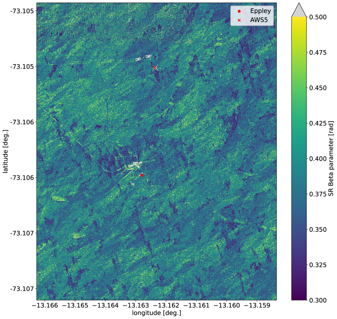
For analysis, the calculated across-track β values were then bucket-resampled on a latitude–longitude grid with a resolution of 0.2 m. The grid extent was drawn for each site from the extent of the drone-imaged and geolocated RGB mosaic of the area. Typical grid-resampled SR data covered areas of ∼1 km2 d–1 (with the drone), containing the albedo measurement site as well as all snow pit locations. Figure 3 illustrates these SR maps over one of our field sites.
Computed surface roughness (β, in radians) over the area surrounding the AWS5 weather station on 12 Jan 2023. The location of the Eppley albedometer is marked with a red circle. Near it, the large β features are the snowmobiles and equipment of the expedition. AWS5 is in the upper center part of the figure (red cross). Near it are two Arctic trucks of Aboa technical crew doing maintenance on the AWS during the day in question. Grid resolution is 0.2 m.

Figure 3 Long description
A map displays computed surface roughness around the AWS5 weather station and Eppley albedometer. The map uses a color scale on the right, labeled 'SR Beta parameter left bracket rad right bracket', ranging from 0.300 to 0.500. The latitude ranges from negative 73.107 to negative 73.105 degrees and the longitude ranges from negative 13.166 to negative 13.159 degrees. The Eppley location is marked with a red circle and AWS5 is marked with a red cross. The map shows varying surface roughness values across the area, with different colors representing different roughness levels.
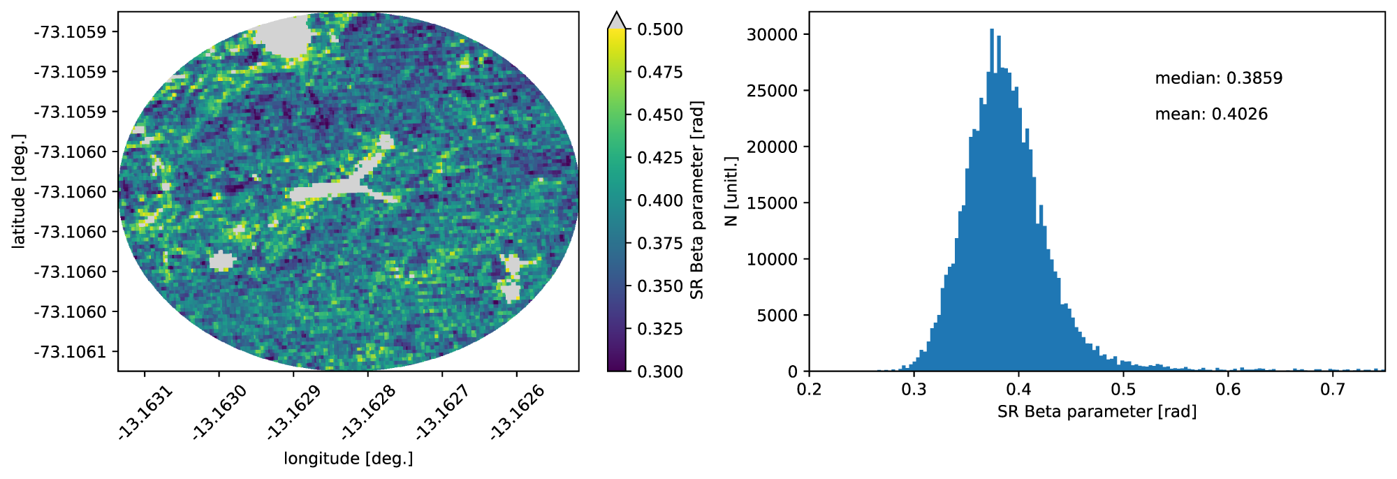
To collocate SR with the observable area of both albedometers, the albedometers were geolocated in each day’s β maps (as in Fig. 3), and the corresponding SR values in a 20 m circle centered on the albedometers (to match the albedometer FOV) were extracted for analysis. Figure 4 shows the output of this processing step for 12 January 2023. To exclude any effects of albedometer mounts, support lines and expedition equipment in the β features extracted over the albedometer FOV, we take the median β as the description of each field site’s and measurement day’s SR to be used in the albedo effect analysis below.
Left, computed β (radians) from a 10 m radius around the Eppley albedometer on 12 Jan 2023 at 0.2 m spatial resolution. Right, the corresponding histogram of β.

Figure 4 Long description
The left image shows a map with latitude and longitude coordinates, displaying a color-coded area with a scale from 0.300 to 0.500 SR Beta parameter in radians. The right image is a histogram of SR Beta parameter values in radians, with the x-axis labeled 'SR Beta parameter [rad]' and the y-axis labeled 'N [unit]'. The histogram shows a peak around 0.4, with a median of 0.3859 and a mean of 0.4026.
2.5. Applying the Gardner–Sharp parameterization for broadband albedo of smooth snow
To model the surface albedo of smooth Antarctic snow, we elected to use the parameterization proposed by Gardner and Sharp (Reference Gardner and Sharp2010), henceforth abbreviated as GS. The parameterization estimates broadband snow surface albedo ( ${\alpha _{{\text{GS}}}}$) as a superimposition of four components, accounting for the effects of snow grain size ( ${\alpha _{\hat S}}$, through SSA), light-absorbing carbon in the snowpack ( ${\text{d}}{\alpha _c}$), albedo changes due to changes in illumination conditions ( ${\text{d}}{\alpha _{u'}}$, SZA) and/or the spectral shift in irradiance under cloudy skies ( ${\text{d}}{\alpha _\tau }$):
 \begin{equation}{\alpha _{{\text{GS}}}} = {\alpha _{\hat S}} + {\text{d}}{\alpha _c} + {\text{d}}{\alpha _{u'}} + {\text{d}}{\alpha _\tau }.\end{equation}
Specifically,
 \begin{equation}{\alpha _{\hat S}} = 1.48 - {\hat S^{ - 0.07}},\end{equation}
where  $\hat S$ is the SSA of snow (cm2 g−1). We form our SSA input as the mean SSA of the top 6 cm of the snowpack(s) measured in the snow pits (Section 2.3) to account for impacts of vertical SSA variability on albedo (Zhou and others, Reference Zhou, Li and Stamnes2003) and acknowledging that the topmost layers are the most crucial when calculating the broadband albedo.
Following prior assessments, which report Antarctic snow to be essentially impurity-free once away from local emission sources such as research station power plants (Kang and others, Reference Kang, Zhang, Qian and Wang2020; Cordero and others, Reference Cordero2022), we treat the albedo effect of carbon as negligible in our data (dαc = 0).
The SZA and cloudiness effects on pure snow albedo are as follows:
 \begin{equation}{\text{d}}{\alpha _u} = 0.53{\alpha _{\hat S}}\left( {1 - {\alpha _{\hat S}}} \right){\left( {1 - u} \right)^{1.2}}\end{equation}
and
 \begin{equation}{\text{d}}{\alpha _\tau } = \frac{{0.1\tau {\alpha _{\hat S}}^{1.3}}}{{{{\left( {1 + 1.5\tau } \right)}^{{\alpha _{\hat S}}}}}},\end{equation}
where u is the cosine of SZA, and τ indicates the cloud optical thickness (COT) of cloud cover over the site. Lacking direct cloud observations, we classified the albedo measurement time series as either clear or cloudy sky (Section 2.2.1) and assigned a climatologically reasonable τ = 10 (Bromwich and others, Reference Bromwich2012) to all cloudy sky observations. Finally, the parameterization treats the effects of an increase in fraction of diffuse irradiance from both increasing SZA and COT as folllows:
 \begin{equation}u' = 0.64x + \left( {1 - x} \right)u,x = {\text{min}}\left[ {{{\left( {\frac{\tau }{{3u}}} \right)}^{0.5}},1} \right].\end{equation}
Thus, Eqn (6) is first applied to modify u in Eqn (4), before its application in Eqn (2). The parameterization is defined over a smooth snow surface without a term to account for SR impacts. We next describe how we attempt to estimate their magnitude in this study.
2.6. Applying the Manninen SR model for snow albedo correction
Manninen and others (Reference Manninen2021) proposed a model for the SR effect on snow albedo. The model constructs a correction term based on SR described through the β parameter, illumination geometry and directionality (SZA, direct/diffuse irradiance fractions), and the albedo of smooth snow. A marked advantage of this model is that the correction term can be added to any modeled smooth snow albedo estimate. Here, we model rough snow (blue-sky) albedo as a combination of the GS parameterization (Section 2.5,  ${\alpha _{{\text{GS}}}}$) and the SR correction ( $\Delta {\alpha _{{\text{SR}}}}$) as follows:
 \begin{equation}{\alpha _r} = {\alpha _{{\text{GS}}}} + \Delta {\alpha _{{\text{SR}}}},\end{equation}
where
 \begin{equation}\Delta {\alpha _{{\text{SR}}}} = f{\alpha _{\text{w}}} + \left( {1 - f} \right){\alpha _{\text{b}}},\end{equation}
i.e., the correction is the diffuse irradiance fraction (f) weighted combination of SR effects on white- ( ${\alpha _{\text{w}}}$) and black-sky ( ${\alpha _{\text{b}}}$) albedos. We use the derived clear-sky fraction (Section 2.2.1) as f. The terms white-sky and black-sky albedo refer to the albedo of the (snow) surface under purely diffuse and purely direct illumination, respectively (Schaepman-Strub and others, Reference Schaepman-Strub, Schaepman, Painter, Dangel and Martonchik2006).
The SR effects are
 \begin{equation}{\alpha _{\text{w}}} = \alpha _{{\text{w}}0}^{\langle n\rangle + 1}\end{equation}
 \begin{equation}{\alpha _{\text{b}}} = {\alpha _{{\text{b}}0}}\alpha _{{\text{w}}0}^{\langle n\rangle }\frac{{\left( {1 - \alpha _{{\text{w}}0}^{\langle m\rangle + 1}} \right)}}{{\left( {1 - \alpha _{{\text{w}}0}^{\langle n\rangle + 1}} \right)}},\end{equation}
where α w0 and α b0 refer to the white- and black-sky albedos of smooth snow (respectively), from Eqns (3–6) for the white-sky case and Eqns (3) and (4) for the black-sky case. These smooth snow albedos are modulated by exponents driven by the average number of facet-to-facet photon scattering events under diffuse (<n>) and direct (<m>) illumination conditions, estimated as described in Section 2.2.1. The model connects <n> and <m> to the measurable SR parameter β through an empirical relationship:
 \begin{align}{n_s}\left( {\beta ,{\text{ }}{\theta _s}} \right) &= 1 + 0.355332\cos \theta _s^4\beta \nonumber\\
&\quad - 1.08275\left( {1 - exp\left( {1.75\cos \theta _s^{1/4}{\beta ^4}} \right)} \right),\end{align}
\begin{align}{n_s}\left( {\beta ,{\text{ }}{\theta _s}} \right) &= 1 + 0.355332\cos \theta _s^4\beta \nonumber\\
&\quad - 1.08275\left( {1 - exp\left( {1.75\cos \theta _s^{1/4}{\beta ^4}} \right)} \right),\end{align}where θ s is the SZA, and
 \begin{equation}\langle m\rangle = {n_s} - 1\end{equation}
 \begin{equation}\langle n\rangle = \frac{{\mathop \sum_{{\theta _{s = 0}}}^{90}\cos {\theta _s}\sin {\theta _s}{n_s}\left( {\beta ,{\text{ }}{\theta _s}} \right) - 1}}{{\mathop \sum_{{\theta _{s = 0}}}^{90}\cos {\theta _s}\sin {\theta _s}}}\end{equation}
So that <n> is essentially the weighted mean of ns across the range of possible SZAs.
3. Results
3.1. Clear-/cloudy sky delineation from observed irradiances and a clear-sky model
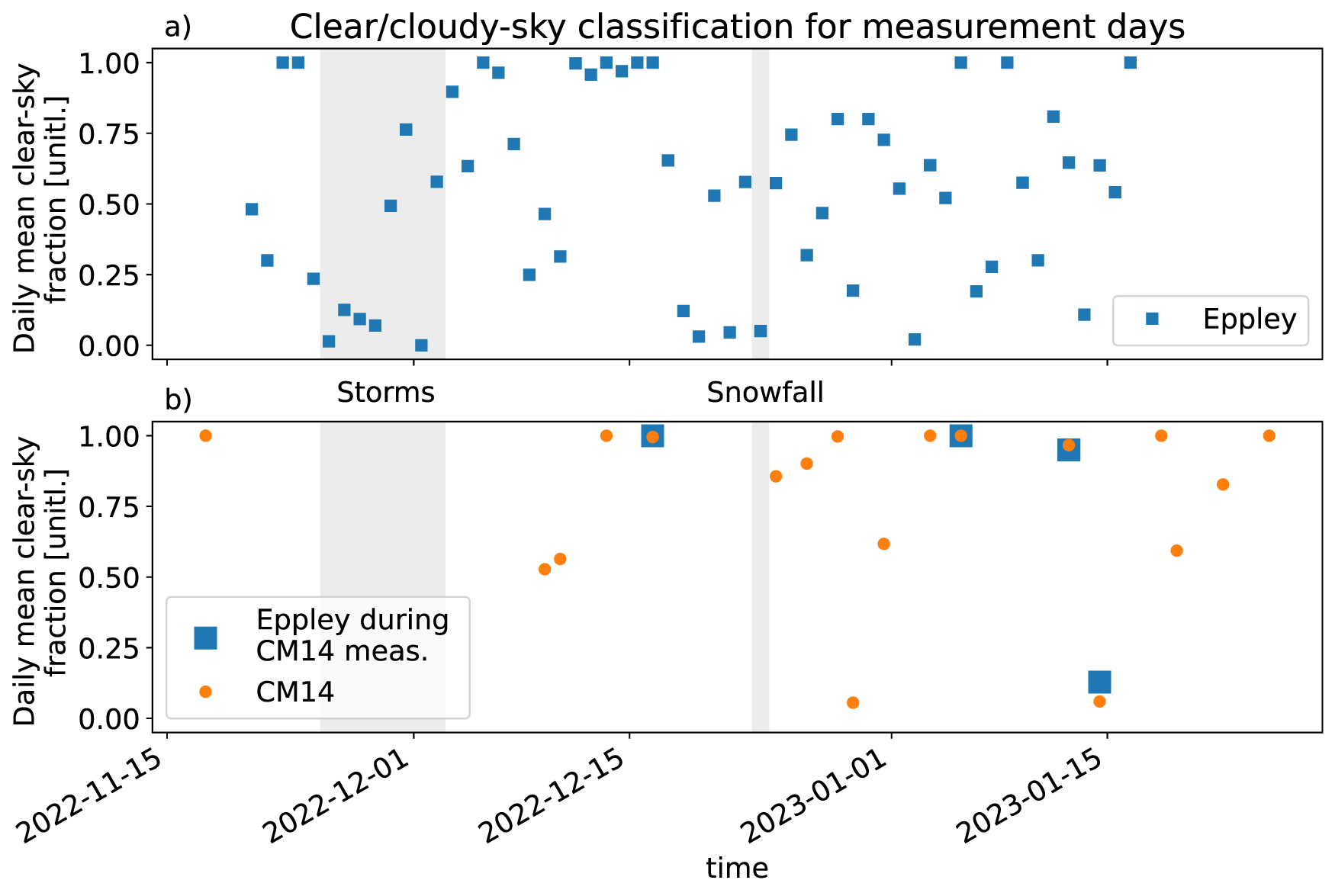
Figure 5 shows the derived daily clear-sky fractions throughout the campaign from the two pyranometers. The early-season storm period (24 November–3 December) manifests as cloudy skies in the Eppley measurements, as expected. The middle part of the campaign was characterized by mainly clear skies, with variable cloudiness during the final third. During days when the field crew visited the AWS5 site where the Eppley albedometer was placed, the coincidentally retrieved clear-sky fractions agreed well (square/circle markers in Fig. 5b). Note that the inclement early-season weather precluded most field operations; thus, the CM14 time series is sparse until mid-December.
Estimated daily clear-sky occurrence fractions from both Eppley (a) and CM14 (b) observations. Overlaid squares in (b) further indicate Eppley clear-sky occurrence during CM14 observation periods on days of collocated observations near AWS5. Early season storm period and mid-season heavy snowfall (observed at Aboa station) events are highlighted in gray.

Figure 5 Long description
The image contains two graphs labeled a and b, showing daily mean clear-sky fraction over time. The x-axis is labeled 'time' with dates from 2022-11-15 to 2023-01-15. The y-axis is labeled 'Daily mean clear-sky fraction [unitless]'. Graph a displays data points using squares representing Eppley measurements, with highlighted periods for storms and snowfall. Graph b shows circles for CM14 data and squares for Eppley during CM14 measurements, also highlighting storm and snowfall periods. Both graphs indicate variations in clear-sky fractions during these periods.
3.2. Parameterization of surface albedo from observed snow SSA and estimated cloudy/clear delineation
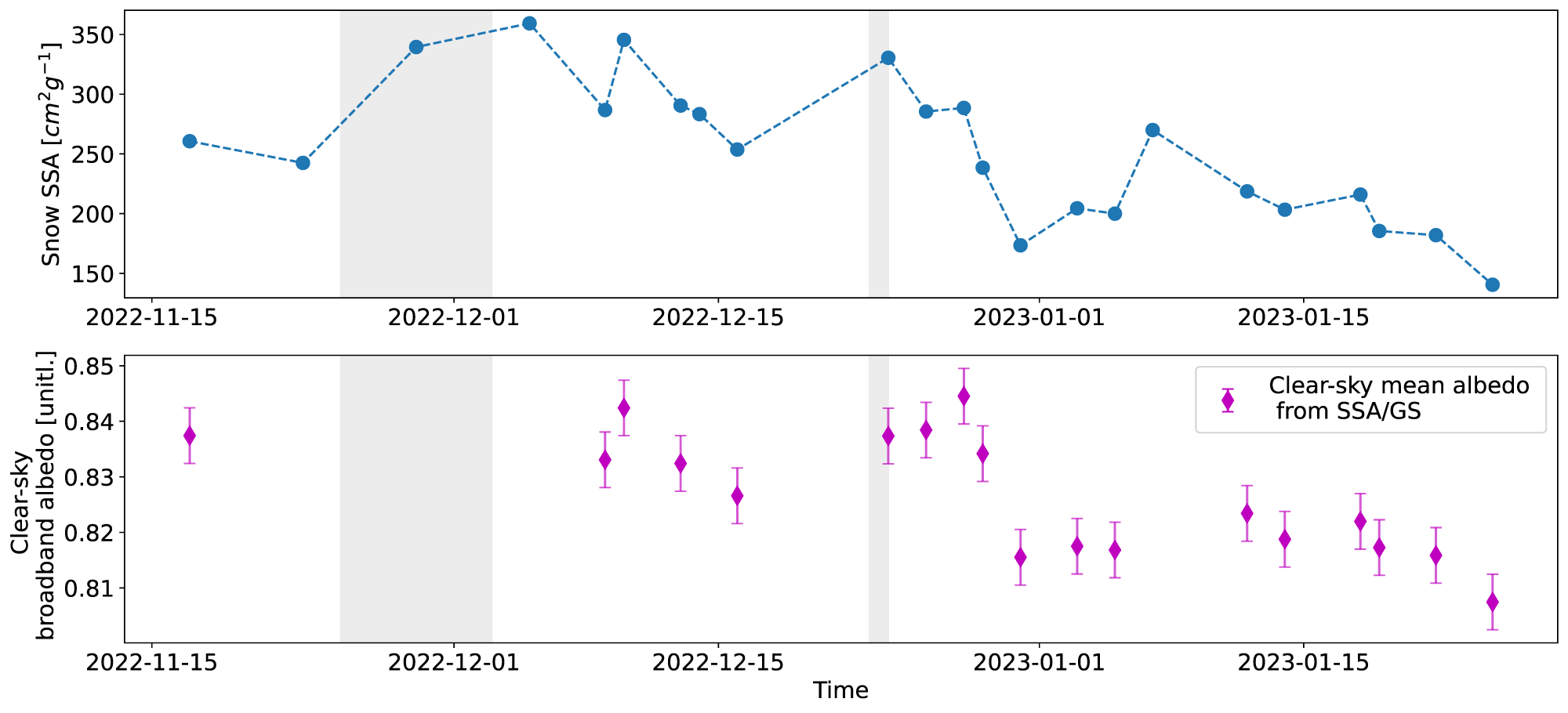
The snow SSA measurements from IceCube were processed as described in Section 2.3. Further, as noted in Section 2.5, the mean SSA of daily samples from the top 6 cm of the snowpack was chosen as the effective SSA to determine the corresponding snow albedo. The parameterized albedos for direct and diffuse illumination were calculated from the GS parameterization (Gardner and Sharp, Reference Gardner and Sharp2010) and combined according to the determined clear-/cloudy sky fractions to form the modeled blue-sky albedo for smooth ice-sheet snow. The obtained daily mean SSA time series is shown in Fig. 6a, with the corresponding modeled clear-sky pure snow albedo (i.e., result of Eqns (3) and (4) without diffuse radiation modification) in Fig. 6b.
(a) Time series of measured specific surface area (SSA) and (b) GS-parameterized (smooth) snow daily mean clear-sky broadband albedo based on SSA measurements and SZA from CM14 observations.

Figure 6 Long description
The first graph shows the specific surface area (SSA) measured in square centimeters per gram from November 15, 2022, to January 15, 2023. The x-axis is labeled 'Time' with dates and the y-axis is labeled 'Snow SSA (cm squared g superscript negative 1)'. The data points are connected by dashed lines, showing fluctuations in SSA values, peaking around early December and decreasing towards mid-January. The second graph displays the clear-sky broadband albedo in unitless measurements over the same time period. The x-axis is labeled 'Time' with dates and the y-axis is labeled 'Clear-sky broadband albedo (unitless)'. The graph includes error bars for each data point, indicating variability in measurements. The albedo values show a slight increase in early December, followed by a gradual decrease. Both graphs have shaded regions indicating specific time intervals.
As expected, both the early-season storms and the mid-season snowfall acted to ‘reset’ the snow surface to consist primarily of fine grains with SSA > 350 cm2 g−1. After precipitation and wind deposition, natural dry-snow metamorphism begins to decrease SSA as snow grains coarsen. The SSA magnitude and temporal evolution are very similar to those observed in the interior of East Antarctica with similar instruments and methods (Libois and others, Reference Libois, Picard, Arnaud, Dumont, Lafaysse, Morin and Lefebvre2015). These physical snow processes are reflected in the evolution of the modeled albedo, though also overlaid with the well-known tendency for snow albedo to increase under cloudy skies due to cloud absorption-driven spectral shift toward visible wavelengths and the change in effective illumination geometry in a diffuse irradiance field (Wiscombe and Warren, Reference Wiscombe and Warren1980).
3.3. Observed surface albedo and SR over Queen Maud Land
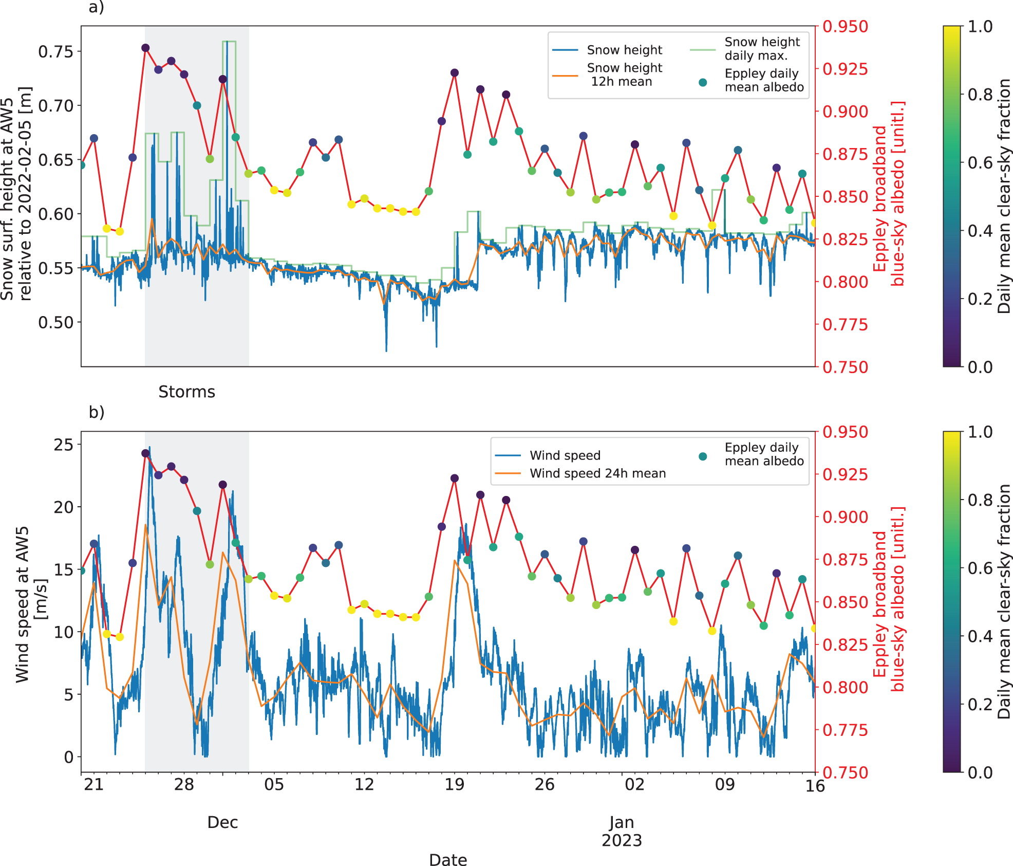
Figure 7 shows the observed time series of surface broadband blue-sky albedo from the Eppley albedometer alongside the snow depth and wind speed observations from the AWS5 weather station in the vicinity. The color of the circular daily mean albedo markers indicates the estimated clear-sky fraction of the day in question. As noted in Section 2.5, snow albedo is expected to increase under cloudy conditions due to spectral and angular modulation of the incoming irradiance, with several of the observed daily mean albedo changes between cloudy and clear-sky days being ∼0.04 to ∼0.06, in accordance with literature-based expectations (Warren, Reference Warren1982; Key and others, Reference R, Wang, C and Fowler2001).
The Eppley time series of daily mean snow albedo overlaid with concurrent AWS5 snow depth change observations (a) and AWS5 wind speed observations (b). Albedo marker color indicates clear-sky occurrence fraction.

Figure 7 Long description
The image contains two graphs labeled a) and b). Graph a) shows snow surface height at AWS5 relative to 2022-02-05 in meters on the left y-axis and Eppley broadband blue-sky albedo on the right y-axis. The x-axis represents dates from December 21 to January 16. The graph includes lines for snow height, snow height 12-hour mean and snow height daily maximum, with markers for Eppley daily mean albedo. The background highlights storm periods. Graph b) displays wind speed at AWS5 in meters per second on the left y-axis and Eppley broadband blue-sky albedo on the right y-axis. The x-axis also spans from December 21 to January 16. It includes lines for wind speed and wind speed 24-hour mean, with markers for Eppley daily mean albedo. Both graphs feature a color scale indicating daily mean clear-sky fraction from 0.0 to 1.0.
Notable albedo increases also occur in late November and ∼17 December, associated with concurrent increases in cloud cover and winds. Winds may significantly influence albedo by depositing small-grained fine snow into the albedometer FOV or by taking it away to expose coarser layers underneath. Daily mean wind speeds and albedo are significantly correlated (Pearson’s r = 0.628, p = 1.31 × 10⁻⁷), supporting the idea that cloudiness and wind-driven surface rearrangement act in concert to modulate albedo variations, overlaid on the slow aging of the surface snow, which gradually decreases albedo after disturbance events (Section 3.2).
Furthermore, the snow depth observations at AWS5 (Fig. 7a, relative to the last AWS5 sensor reset in February 2022) reveal a net change of only ∼2 cm during the campaign period, further supporting the argument that wind-blown snow was the major driver of surface snow change rather than fresh snow from precipitation (at AWS5). Indeed, sub-daily variations of up to 20 cm were observed by the snow depth sensor during the early season storms, though quickly dispersed and smoothed by the strong winds. Frezzotti and others (Reference Frezzotti2004) reported, based on prior works such as Kobayashi and Ishida (Reference Kobayashi and Ishida1979), that a wind speed threshold of 13–14 m s−1 defines the boundary between low-altitude drifting and high-altitude blowing snow, and that a threshold of 15 m s−1 typically separates the wind-driven surface feature production between depositional features such as waves or barchans and redistribution features such as sastrugi. Our data confirm that nearly all 10 min snow surface height variations larger than ±2 cm occur with wind speeds larger than 13 m s−1, consistent with prior studies.
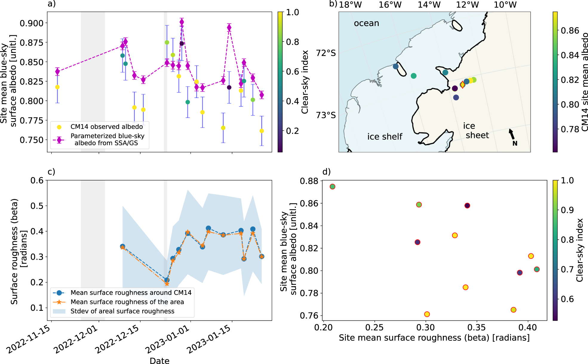
Turning to the observations from the roving CM14 albedometer, Fig. 8a shows the measured mean albedos from each field site, overlaid with corresponding parameterized blue-sky albedos from the GS parameterization. Contrasting with Fig. 6b, here the estimated clear-sky fraction from CM14 data (Section 2.2.1) is used to combine the parameterized black- and white-sky albedos to compare with the albedometer observations. The temporal variability in observed site-mean blue-sky albedos (ranging between 0.76 and 0.87) is similar to that seen with Eppley, though somewhat amplified as the field site changed daily. Here, the parameterized albedo shown is valid for a smooth snow surface.
Figure 8b shows the locations and measured mean blue-sky albedos of the principal field sites (with collocated laser scanner and CM14 data) in the region surrounding Aboa station. Two of these sites were on the Riiser-Larsen Ice Shelf (visited on 28 December and a site on its edge on 31 December). The locations were chosen to coincide with ICESat-2 and CryoSat-2 overpasses to verify their elevation estimates and to study the effects of SR on the satellite altimeter measurements (Leppänen and others, Reference Leppänen, Kukko, Rimali, Riihelä and Tisler2025).
The daily mean snow albedo time series from CM14 (circles) and the corresponding parameterized smooth snow albedos (diamonds) in (a), the spatial distribution and site mean albedos of principal CM14 sites, with the Eppley site marked with a diamond in (b), the retrieved mean surface roughness (β) in the approximate FOV of CM14 (blue circles), the area-mean β (orange stars) and the ±1 SD of the areal surface roughness (blue shaded area) in (c), and the correlation of surface roughness and the corresponding site-mean snow albedo from CM14 in (d). Albedo marker color in (a) and (d) indicates the mean clear-sky fraction during each day’s observation period. Ice-shelf edge from the SCAR Antarctic Digital Database, 2024.

Figure 8 Long description
The image consists of four panels. Panel a shows a line graph with the x-axis labeled 'Date' and the y-axis labeled 'Site mean blue-sky surface albedo [unitless]'. It displays CM14 observed albedo (yellow circles) and parameterized blue-sky albedo from SSA/GS (purple diamonds) over time from 2022-11-15 to 2023-01-15. Panel b is a map showing the spatial distribution of CM14 site mean albedo with locations marked on an ice sheet and ocean. Panel c presents a line graph with the x-axis labeled 'Date' and the y-axis labeled 'Surface roughness (beta) [radians]'. It shows mean surface roughness around CM14 (blue circles) and mean surface roughness of the area (orange stars) with a shaded area representing the standard deviation. Panel d is a scatter plot with the x-axis labeled 'Site mean surface roughness (beta) [radians]' and the y-axis labeled 'Site mean blue-sky surface albedo [unitless]'. It shows the correlation between site mean surface roughness and albedo, with color indicating the clear-sky index.
Following the steps outlined in Section 2.4, the SR of the snow was extracted from the laser scanner data over each site’s albedometer FOV. The resulting mean RMS slope (β) parameter at the 20 cm spatial scale is shown in Fig. 8c. The range in β (0.21–0.41 rad, i.e., 12–24°) indicates a rougher snow surface than has been observed for boreal seasonal snow (Manninen and others, Reference Manninen2021). The roughness values in the albedometer FOV closely resembled the overall mean SR of the drone-imaged areas around the measurement sites. It is important to recall that the SR description is scale-dependent; we will return to the topic in Section 4. Interestingly, the lowest measured SR values (both mean and SD) occurred immediately after a snowfall event (23 December) without heavy winds in the region (Fig. 5b). Thus, conditions were likely suitable for a smooth new surface snow layer to have been deposited just prior to the laser scanning on 24 December.
As a qualitative first test for the darkening effect of snow SR on the observable albedo, we plotted the CM14 blue-sky albedos against the laser scanner-based mean β of the instrument FOV. The results (Fig. 8d), though noisy in part due to the cloudiness-induced variation in albedo, which plays no role for SR retrieval, still indicate the presence of the expected negative correlation (r = −0.54, p = 0.08).
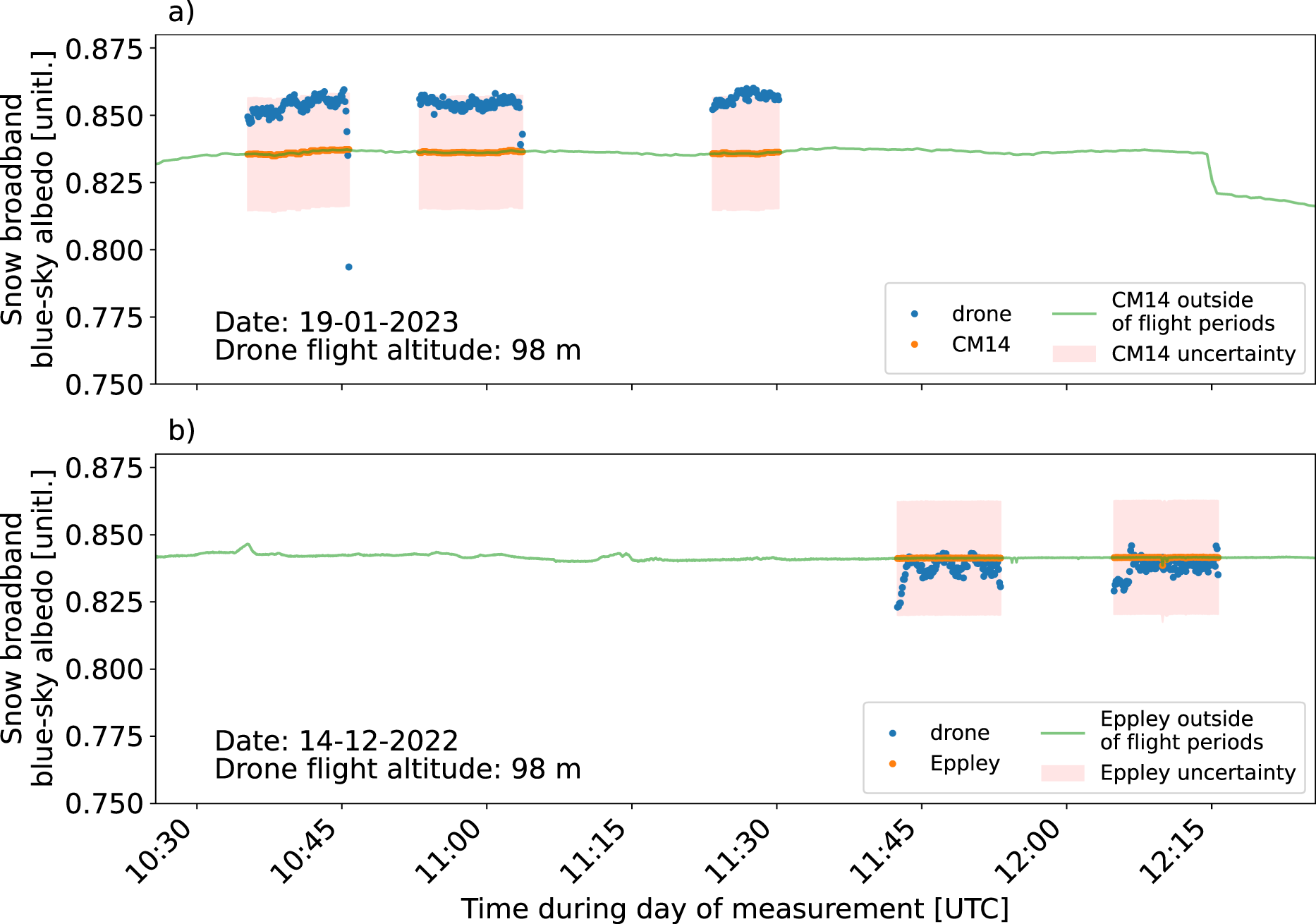
An additional verification of the ground-based albedo observations is available through a comparison with the airborne albedo measurements described in Section 2.2.2. Figure 9 illustrates a comparison between the UAV-based albedo estimate and the ground observations from both CM14 and Eppley. In this example, three flights took place in the area surrounding the CM14 measurement site on 19 January 2023 (Fig. 9a), and two flights observed the areal albedo of the Eppley site on 14 December 2022 (Fig. 9b). Each flight was limited to ∼15 min by the battery capacity of the UAV. As the irradiance data for the UAV-based estimate are drawn from the ground instruments, the observations cannot be considered fully independent. However, the reflected fluxes measured from the sky agree with their ground-based counterparts within the observational uncertainty of the overall albedo measurement. The somewhat larger variability in the UAV-based estimate is partly due to spatial variability in the snow albedo, as only a part of the flight path is collocated with the ground observation, and partly due to residual imperfections in the UAV’s downward-pointing pyranometer leveling despite the gimbal stabilization.
Examples of drone-based snow broadband albedo against ground-based albedo measurements from (a) CM14 on 19 Jan 2023 and (b) Eppley on 14 Dec 2022. Both days were verified by the field crew as fully clear-sky. The shaded area indicates the estimated 5% measurement uncertainty range of the ground-based albedometers.

Figure 9 Long description
The image contains two graphs comparing drone-based and ground-based snow broadband blue-sky albedo measurements. Graph a) shows data from 19-01-2023 with a drone flight altitude of 98 meters. The x-axis is labeled 'Time during day of measurement [UTC]' ranging from 10:30 to 12:15. The y-axis is labeled 'Snow broadband blue-sky albedo [unitless]' ranging from 0.750 to 0.875. Blue dots represent drone measurements, orange dots represent CM14 measurements and a green line indicates CM14 measurements outside flight periods. A shaded area shows CM14 uncertainty. Graph b) shows data from 14-12-2022 with the same drone flight altitude. The x-axis and y-axis labels are identical to graph a). Blue dots represent drone measurements, orange dots represent Eppley measurements and a green line indicates Eppley measurements outside flight periods. A shaded area shows Eppley uncertainty.
3.4. Applying the SR correction to parameterized smooth snow albedo
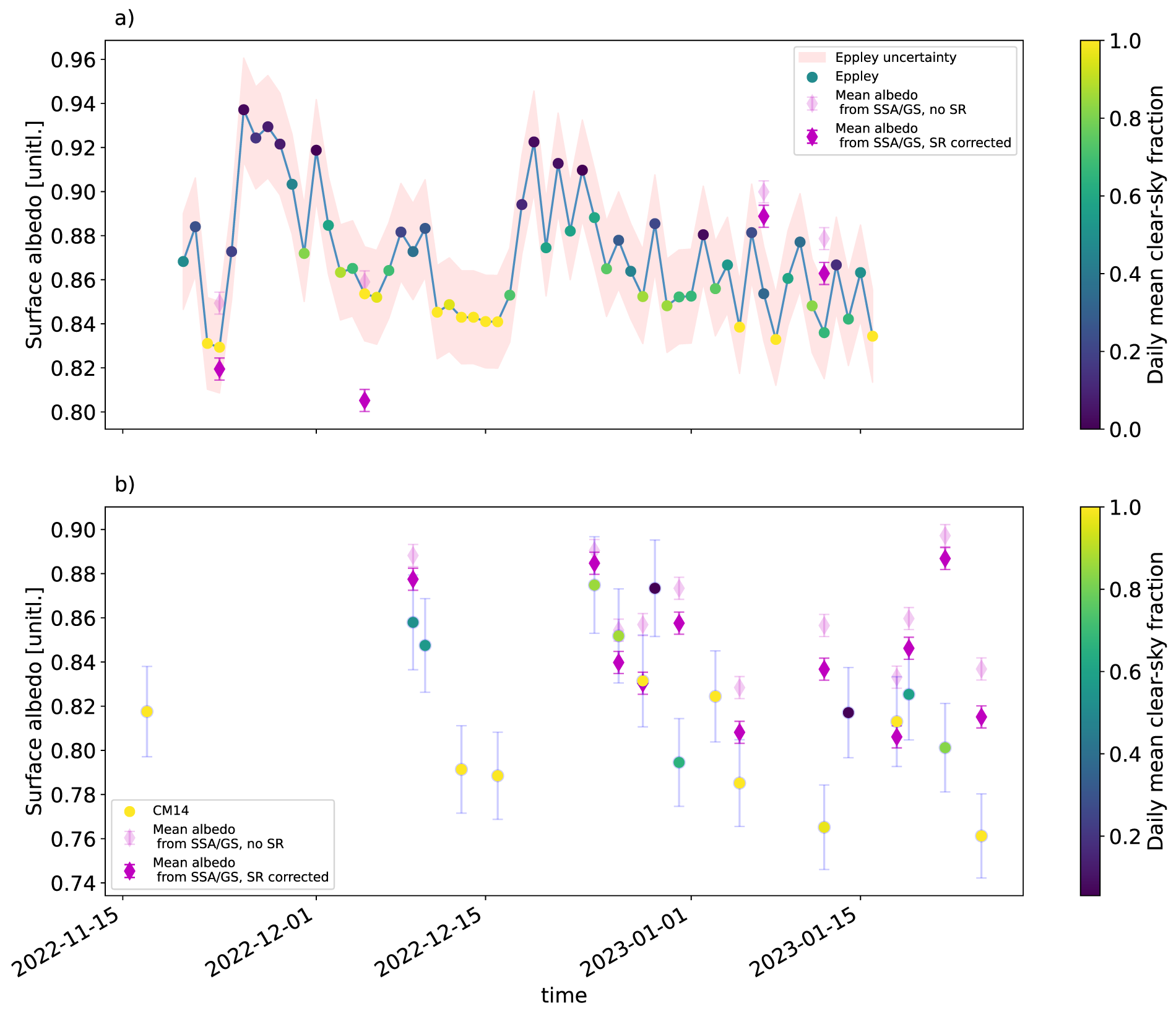
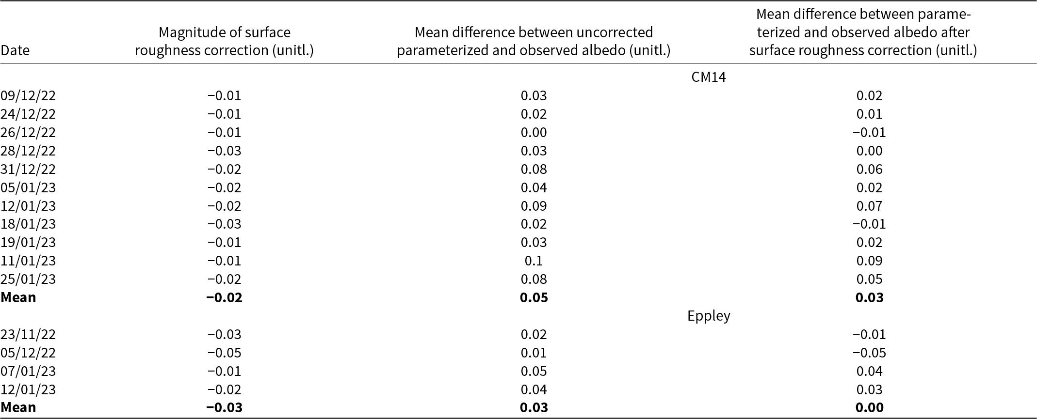
We used the Manninen model (Section 2.6) to estimate the change in blue-sky albedo associated with the observed roughness of the snow surface for the 11 CM14 field sites as well as 4 days when the laser scanner UAV flew over the Eppley measurement area near AWS5. We then applied the correction to the parameterized blue-sky albedos (Section 2.5) to see if the correction improved the agreement between measured and parameterized albedos. The results are shown in Fig. 10 and listed in Table 3.
The effect of applying the surface roughness (SR) correction to smooth snow albedo from GS parameterization is shown against observations from (a) Eppley and (b) CM14.

Figure 10 Long description
The image A shows a line graph with surface albedo on the y-axis (unitless) and time on the x-axis, ranging from November 15, 2022, to January 15, 2023. It includes data points for Eppley observations, mean albedo from SSA/GS without SR and mean albedo from SSA/GS with SR correction. Eppley uncertainty is shown with a shaded area. The daily mean clear-sky fraction is indicated by color. The image B shows a scatter plot with the same axes. It includes CM14 observations, mean albedo from SSA/GS without SR and mean albedo from SSA/GS with SR correction. Error bars are present for each data point and the daily mean clear-sky fraction is also indicated by color.
Impact of surface roughness correction on the difference between parameterized and measured albedo from the CM14 and Eppley observations.

Table 3 Long description
The table measures the impact of surface roughness correction on the difference between parameterized and observed albedo for CM14 and Eppley observations. For CM14, the correction consistently reduces the mean difference, with values ranging from 0.03 to 0.09 unitl. before correction and 0.00 to 0.09 unitl. after correction. The mean difference for CM14 decreases from 0.05 to 0.03 unitl. post-correction. For Eppley, the correction also reduces the mean difference, with values ranging from 0.01 to 0.05 unitl. before correction and -0.05 to 0.04 unitl. after correction. The mean difference for Eppley drops from 0.03 to 0.00 unitl. after correction. The data suggests that surface roughness correction generally improves the accuracy of parameterized albedo measurements.
The correction acts to always lower the parameterized albedo, as expected (Manninen and others, Reference Manninen2021), and appears to improve the match between parameterized and measured albedo for CM14, with the mean difference decreasing from +0.05 to +0.03. On 10 out of 11 field sites, the match is better after the derived SR correction. Three notable outlier days exist where the observation-parameterization bias is large both before and after the SR correction (31 December 2022, 12 January 2023 and 22 January 2023). Based on visual inspection of the irradiance measurements, we find that the likely cause is the use of a climatological COT estimate due to the lack of cloud property measurements. Using a static COT = 10 implies the assumption of an optically thick cloud cover, which, for cases with existing but thin cloud cover (as occurred on these days), will overestimate the cloudiness-induced increase in parameterized snow albedo.
For Eppley, the results are similar, although with 5 December as a particular outlier in terms of estimated SR impact. If that day were disregarded, the mean correction magnitude at the Eppley site would be −0.02, in line with the CM14 sites. We analyze possible causes for these deviations and provide an extended uncertainty analysis in the following discussion.
4. Discussion
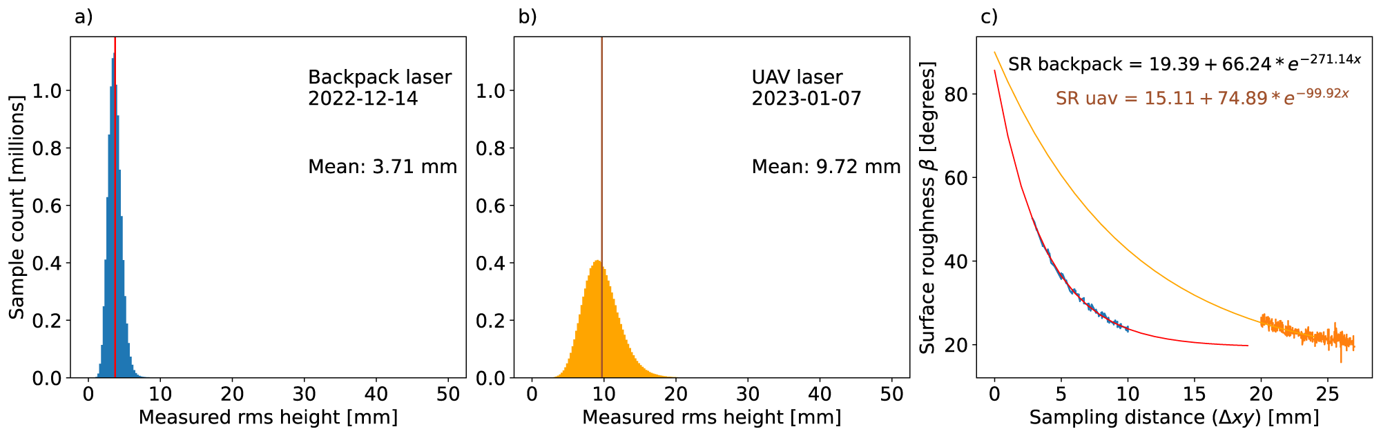
SR descriptions are typically scale-dependent (Fassnacht and others, Reference Fassnacht2023). The question therefore is, whether our results would change significantly if different choices were made regarding the spatial resolution used to determine β? To explore this issue, a set of supporting laser scanner observations was made during the campaign with a separate backpack-mounted laser scanner (Riegl VUX-1HA). As the scanner’s measurement height is ∼2 m, the setup allows for millimeter-scale ground sampling in the resulting laser point cloud. These, data, available from 3 days (13 December, 14 December, and 16 December 2022), were processed with the methods described in Section 2.4.
Figure 11a shows the distribution of measured RMS height variations with the backpack laser scanner on 13 December 2022 (a random sample of the day’s data, N = 10 × 106). The variation range (∼2–6 mm) is in good agreement with similar measurements on a glacier in Svalbard (Lacroix and others, Reference Lacroix2008). Corresponding distributions measured with the UAV-mounted laser scanner on 7 January 2023 (as an example) in Fig. 11b are clearly larger, with a mean of 9.72 mm and a variation range of ∼5–16 mm (2–98% of distribution).
(a) RMS heights measured with the backpack laser scanner (VUX-1HA) on 14 December 2022, (b) RMS heights measured with the UAV-mounted laser scanner (VUX-120) on 7 January 2023 and (c) surface roughness (SR) parameter β obtained from both laser scanner measurements as a function of sampling distance in the laser point cloud. Solid lines indicate physically constrained best-fit exponential functions following the formulation in Manninen and others (Reference Manninen2021).

Figure 11 Long description
The image consists of three graphs. Graph a shows the sample count in millions on the y-axis and measured RMS height in millimeters on the x-axis, using a backpack laser on 14 December 2022. The mean RMS height is 3.71 millimeters. Graph b displays similar data using a UAV laser on 7 January 2023, with a mean RMS height of 9.72 millimeters. Graph c illustrates surface roughness beta in degrees on the y-axis against sampling distance delta xy in millimeters on the x-axis. Two exponential functions are shown: SR backpack equals 19.39 plus 66.24 times e superscript negative 271.14x and SR UAV equals 15.11 plus 74.89 times e superscript negative 99.92x.
However, it should be kept in mind that the UAV sampling distances in the laser point cloud are also considerably larger. Figure 11c illustrates the derived mean β as a function of spatial distance and associated best-fit exponential functions from both sensors. The fitted functions as well as the cutoff limits for spatial distance have been chosen to correspond with those used in Manninen and others (Reference Manninen2021) to facilitate a comparison. For the UAV, the spatial distance range shown corresponds to the 20–80% variation range in the point-to-point distances in the laser point cloud.
The level where SR stabilizes with coarsening sampling distance (19°, i.e., 0.33 rad) in the backpack measurements is clearly similar to that observed from the UAV-mounted laser scanner (15°, i.e., 0.26 rad). However, the best-fit exponential curves are notably different. Here, the best-fit inversion was made with physical constraints, i.e., β cannot exceed 90°. Compared to boreal seasonal snow (Manninen and others, Reference Manninen2021), the Antarctic snow surface thus appears substantially coarser, which is expected. Whether or not the exponential fits are accurate in the 1–3 mm scale would require verification with independent observations. In the prior study of Manninen and others (Reference Manninen2021), high-precision graded plates were inserted into the snow and photographed to achieve submillimeter-scale SR estimation. However, the hard surfaces of Antarctic snow make graded plate insertions very difficult to achieve without destroying the surface itself, and they were, therefore, not attempted during our campaign. The question of quantifying submillimeter-scale SR thus falls out of scope for this study.
To assess whether or not the SR correction on parameterized blue-sky albedo statistically improves the agreement against the albedometers, we performed paired t tests separately against the CM14 and Eppley observations. Both corrected and uncorrected parameterized albedos showed statistically significant bias against CM14 observations (p < 0.01), with the t value showing a decrease after SR correction was implemented (101 vs 59). Furthermore, testing these biases against each other showed that they are significantly different (p < 0.01). The sample size of the CM14 dataset was N = 6566, suggesting that the test statistics are robust in terms of sufficient sampling size. For Eppley, the statistics also confirm the significance of the difference after the correction (p < 0.01), but the t values are notably different (134 vs −158). For the continuously operated Eppley radiation station, the sample size is much larger at N = 81 540 (30 s periods, SZA < 70°).
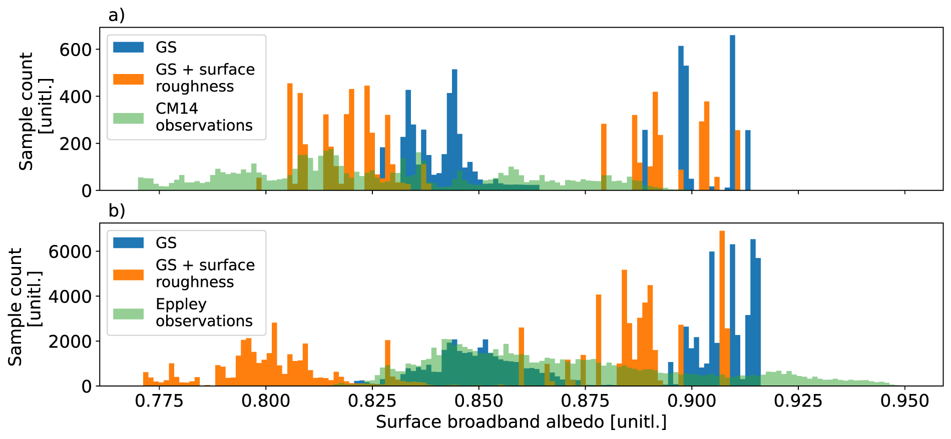
Figure 12 illustrates the distributions of observations arrayed against the parameterized albedos with and without the SR correction. The bimodal nature of the parameterized albedo results from the sharp change between periods identified as cloudy or clear-sky, given the climatological COT applied during the parameterization. It should further be kept in mind that the CM14 distribution is a composite over all different field sites, whereas the Eppley measurements reflect variability in time over a fixed location. As reflected in the t test statistics, it is apparent that for CM14, the inclusion of the correction improves both cloudy and clear-sky albedo matches to observations, whereas for Eppley, it can often lead to an underestimation.
Observed (light green) and GS-parameterized surface broadband snow albedos with surface roughness correction (orange) and without it (blue). Measured albedo source for top subplot: CM14, bottom: Eppley.

Figure 12 Long description
The image contains two bar graphs labeled a) and b). Graph a) shows sample counts of surface broadband albedo for GS, GS with surface roughness correction and CM14 observations. The x-axis is labeled 'Surface broadband albedo [unitless]' and ranges from 0.775 to 0.950. The y-axis is labeled 'Sample count [unitless]' and ranges from 0 to 600. Graph b) presents similar data for GS, GS with surface roughness correction and Eppley observations. The x-axis is the same as graph a), while the y-axis ranges from 0 to 6000. Both graphs illustrate the distribution of albedo values with distinct peaks and variations across the different datasets.
Overall, on a day-to-day basis, applying the SR correction in the parameterized smooth snow albedo improved the agreement with measured albedo in the majority of cases (13 out of 15 analyzed days of observations). Some notable data outliers and analysis assumptions deserve further examination.
First, the laser measurements on 05 December 2022 yielded an unusually large β (0.58 rad) over the Eppley FOV, leading to a markedly large albedo correction during a day when the parameterization for smooth snow albedo already yielded very good agreement with observations. Although consistent with the mean β over the whole laser-scanned area on that day (not shown), the usually coarse surface seems out of place in the context of the rest of the observed β time series. The field crew observed snow accumulation against the Eppley supports, which may alter the local effective geometry of the surface and lead to over- or underestimation of observed albedo relative to level horizontal snow, depending on the tilt and orientation of the accumulation surface. Unfortunately, the albedometer mounting interfered with the UAV laser scanning (Fig. 4a) to a degree that prevents us from quantifying the effect. In future efforts, scanning the albedometer FOV with, e.g., backpack-mounted laser scanners could yield better information about the effects of wind-blown snow on the observed albedo.
Second, as noted earlier, the assumption of optically thick clouds during periods of cloud cover is clearly detrimental in cases where actual conditions are those of thin or broken cloud cover. Studies such as Boers and others (Reference Boers, Van Lammeren and Feijt2000) have shown that accurate determination of cloud optical properties from ground observations requires observations of cloud fraction and the availability of cloud lidars and microwave radiometers to sample the total column liquid water and cloud vertical structure. Lacking these, we observed that our parameterized albedos were subject to considerable overestimation during days of thin or mixed clouds.
Our calculations of parameterized smooth snow albedos were made under the assumption that the snow is pure, i.e., impurity concentrations are negligible. While the gas-fired generator at Aboa station does produce impurity emissions, none of the field sites here were closer to the station than 6.6 km (Table 1). In the impurity measurements of Casey and others (Reference Casey, Kaspari, Skiles, Kreutz and Handley2017) around the South Pole station, black carbon loading decreased to very low amounts with (upwind) distances >1 km from emission sources. Given the much larger distances here, the assumption of snow purity seems warranted. We acknowledge that we did not carry out snow impurity measurements during the campaign; thus, this element remains an assumption in the analysis.
Our results focus on the albedo effects of millimeter-to-centimeter SR, and thus, one is tempted to ask if we are missing a substantial fraction of the total effect across scales by not explicitly considering, e.g., sastrugi effects? The expedition crew reported that there were few large-scale sastrugi present during the 2022–23 field season in the region of Aboa station (compared to, e.g., 2014, when one member of the field crew [Leppänen] was also present). We postulate that pre-field season snowfalls and wind redistribution acted to smooth out prominent sastrugi before our measurements. Also, due to the need to level the albedometers carefully, the field crew generally sought out as level snow as possible. Combined, these factors would have minimized sastrugi and other macroscopic snow roughness features in the albedometer FOV and thus diminished their impact on the analyzed data.
Verification of the ground-mounted albedo measurements with UAV-mounted downward-pointing pyranometer showed that both albedometers were consistent with airborne observations within the measurement uncertainty limits (Fig. 9), and, therefore, we cannot discard any of the observations as unrealistic. In general, verification of the small-scale SR effects on snow albedo is challenging, as the typical magnitudes of said effect are often smaller or equivalent to the measurement uncertainty itself. However, the SR and albedo we have measured and reported here in Queen Maud Land are consistent with prior theory and observations, and in the majority of the observed snow surfaces, the SR correction does improve the agreement between parameterized but observation-driven smooth snow albedo and reference snow albedo observations.
5. Conclusions
We present an analysis of the observed SR of Antarctic snow and its modeled impact on snow broadband albedo. We first report on a series of measurements of snow optical properties, surface albedo and SR, made across a variety of field sites in Queen Maud Land, Antarctica, during the austral summer of 2022–23. The collocated measurements were based on the combined use of UAV- and ground-mounted sensors to achieve both precision and areal coverage. While inclement weather limited operations during the early part of the field season, a total of 15 field sites were visited during the campaign. The locations were selected to coincide with CryoSat-2 and ICESat-2 overpasses to enable examinations of SR effects on altimeter observations (Leppänen and others, Reference Leppänen, Kukko, Rimali, Riihelä and Tisler2025).
The observed snow optical properties and albedo aligned well with prior measurements in the region and displayed consistency with the weather conditions observed by the field crew (snowfall, wind drift effects). To our knowledge, few prior measurements of snow SR at millimeter-to-centimeter scales exist on the Antarctic margins. Our observations displayed RMS heights consistent with similar measurements of Arctic glacier snow at ground level. The RMS heights obtained from the UAV-mounted laser scanner were larger, yet both data sources displayed convergence toward similar RMS slope angle (β) at our baseline spatial resolution scale of 20 cm. At that resolution, the RMS slope angle variation range at our field sites was between 0.183 and 0.559 rad (5–95% of all data, N = 3.5 billion, mean = 0.36 rad).
In the second part of our analysis, we derived parameterized smooth snow albedo based on measured snow-specific surface area and estimated direct/diffuse illumination proportions. We then corrected these parameterizations with the SR model of Manninen and others (Reference Manninen2021), using laser-scanned SR as input, to see if the correction improves or degrades the agreement between measured and parameterized snow albedo. We find that the agreement improves with the correction in the majority, though not all, of our observations. Further, the typical range of SR effect on snow albedo given our data (0.01–0.02) aligns well with expectations based on literature (Warren and others, Reference Warren, Brandt and O’Rawe Hinton1998; Larue and others, Reference Larue2020).
Despite the generally positive results, we acknowledge that the magnitude of the small-scale SR effect on broadband albedo is minor enough to often fall within the observational uncertainty bounds, thus making it difficult to assess whether our SR model or its numeric components are optimal for ice-sheet applications. Our study focused by design on the small-scale SR effects and did not consider measurements made at very low Sun elevations, where the impacts of both macroscopic and millimeter-scale SR features would be amplified. The results obtained were also likely affected by the annual variation of snow surface conditions over our study region; the field crew reported a general lack of sastrugi based on visual observation, which we postulate having resulted from substantial pre-campaign snowfalls and/or wind redistribution. This would have led to the small-scale SR effects being far more apparent than macroscopic ones in our data, regardless of analysis method.
In the future, efforts to achieve still greater radiometric precision in the albedo measurements would serve well to draw down the uncertainty envelopes in the analysis and address the limitation discussed above. A promising direction would be to use carefully calibrated, high-quality and gimbal-stabilized pyranometers on heavy-duty UAVs with sufficient carrying capacity and inertial mass to ensure stability of measurements in flight. In principle, hovering measurements from such platforms at altitudes of a few meters above the snow surface could replace ground-mounted albedometers and circumvent uncertainty sources such as mounting-support shading or snow-drift accumulation. We also note that the measurement design should also guard against inadvertent disturbance of the snow surface through propeller downwash. Also, multiscale analysis of data gathered over prominent sastrugi fields would serve to better delineate the relative magnitudes of macroscopic and millimeter-to-centimeter-scale SR effects on snow albedo.
Data availability statement
A curated selection of laser scanner data along with all measured snow albedos and optical properties are available at https://doi.org/10.57707/fmi-b2share.900cf0c74c1c45efb396b910a841bb3c. The associated principal analysis codes applied are also available upon request.
Acknowledgements
The work of all authors has been financially supported by the Research Council of Finland, decision #335986 (LAS3R). The authors would like to acknowledge the invaluable logistical and operational role of the Finnish Antarctic Research Program FINNARP in maintaining Aboa research station for scientific research. The authors would also like to thank Kari Mäenpää at the FMI-ARC research center for his valuable work in designing and building the UAV radiometric measurement systems.
Author Contributions
Riihelä conceived the study, carried out the principal analyses, and wrote the majority of the manuscript. Rimali performed the radiometric UAV measurements and contributed to the manuscript text. Kukko performed the laser scanner measurements, contributed to their (pre)processing, and to the manuscript text. Litkey and Lehtomäki carried out the processing of laser scanner data into point clouds and RMS heights and contributed to the manuscript text. Leppänen carried out the in situ albedo measurements, the snow SSA measurements, and contributed to the manuscript text.
Competing Interests
The authors declare that they have no conflict of interest.

 Open access

