


1. Introduction
There are 2 principles of decision making that are regarded by many, but not all, theoreticians as rational: dominance and transitivity. Dominance is the principle that if option A yields consequences that are at least as good and sometimes better than the corresponding consequences for option B for every state of the world, then one should prefer option A over B. Transitivity holds that if one prefers X to Y and Y to Z, then one should prefer X to Z.
Transitivity and dominance are not only widely regarded as rational, they are also implied by certain descriptive theories of decision making such as expected utility (EU) theory and cumulative prospect theory (Tversky and Kahneman, Reference Tversky and Kahneman1992). However, other descriptive theories of risky decision making satisfy transitivity but can violate dominance, such as the transfer of attention exchange (TAX) and rank-affected multiplicative weights models (Birnbaum, Reference Birnbaum2008). Another group of theories can violate transitivity and must satisfy dominance, such as the most probable winner (MPW) model (Blavatskyy, Reference Blavatskyy2006; Butler and Blavatskyy, Reference Butler and Blavatskyy2020; Butler and Pogrebna, Reference Butler and Pogrebna2018) and regret theory (Loomes and Sugden, Reference Loomes and Sugden1982). Therefore, testing dominance and transitivity empirically allow psychologists to learn which models can be ruled out or retained as possible descriptive theories of how people actually make decisions.
1.1. Background and purposes of the present study
Butler and Pogrebna (Reference Butler and Pogrebna2018) constructed a set of choice problems in which systematic violations of transitivity were observed. Their design used sets of 3 gambles (‘triples’) with 3 equally likely cash prizes. For example: X = (15, 15, 3), Y = (10, 10, 10), and Z = (27, 5, 5), where X = (15, 15, 3) represents a gamble with 2 equal chances to win 15 pounds and 1 equal chance out of 3 to win 3 pounds. The choice problems were designed such that every choice compared a ‘safer’ option (with lower range of outcomes) against a ‘riskier’ alternative (higher range) that had a higher expected value.
They were also devised such that X has better outcomes than Y for 2 of 3 branches, Y beats Z on 2 branches, and Z beats X on 2 branches. If people choose gambles that are most likely to give a better outcome, called the MPW strategy, they would choose X over Y, Y over Z, and Z over X, violating transitivity. Although their experiment was designed to investigate this MPW model, and some violations of this type were observed, Butler and Pogrebna (Reference Butler and Pogrebna2018) reported that their results showed more violations of the opposite type from those implied by MPW. Birnbaum (Reference Birnbaum2020) reanalyzed those data via the group true-and-error (TE) model and concluded that 4 of the 11 triples showed evidence of small but significant violations of transitivity (Butler, Reference Butler2020).
These 4 triples were later tested in a new study with 22 individuals who responded 60 times to each choice problem (Birnbaum, Reference Birnbaum2023a), which allowed analysis via the individual TE model. Birnbaum (Reference Birnbaum2023a) concluded that although most individuals satisfied transitivity, 1 person showed violations consistent with the MPW model, and 6 others showed evidence of intransitive behaviors in at least one of the triples at least part of the time.
Birnbaum (Reference Birnbaum2023a) also tested dominance using test trials interspersed among the transitivity trials and found surprisingly high rates of violation by some individuals. There were 5 participants who violated transparent dominance more than half the time, including 2 who violated dominance 60 times out of 60 tests despite being almost perfectly self-consistent and transitive in their responses on 720 other trials with non-dominated choices.
In Birnbaum’s (Reference Birnbaum2023a) dominance tests, a low-variance alternative was always dominated by a higher-variance alternative. All 5 of the participants who violated dominance systematically preferred ‘safe’ (low-variance) alternatives on other choice problems not involving dominance. It was conjectured that the experimental design testing transitivity may have induced a strategy in some individuals to look for the ‘safe’ alternative, which left them vulnerable to violating dominance in tests where the low-variance, ‘safe’ alternative was dominated. It was hypothesized that if choice problems were used in which the ‘safe’ alternative was dominant, these people would likely satisfy dominance (Birnbaum, Reference Birnbaum2023a).
This article builds on the designs of Butler and Pogrebna (Reference Butler and Pogrebna2018) and Birnbaum (Reference Birnbaum2023a) to test this new hypothesis about dominance violations and to reassess evidence of intransitive preferences, as measured by a more general TE model than has been employed in previous research on transitivity. The more general model allows 2 error rates per choice problem instead of 1. This study investigates (1) whether violations of transitivity observed by Butler and Pogrebna (Reference Butler and Pogrebna2018) and Birnbaum (Reference Birnbaum2023a) can be observed with a new, larger sample in order to check the estimated incidence with the more complex TE model; (2) whether the rate of violation of transparent dominance will be significant and higher among persons who most often prefer low-variance gambles (as previously reported); and (3) whether the rate of dominance violations would be lower in new tests of dominance in which the lower-variance alternative dominates the higher-variance alternative (compared against the case in which the dominant gamble has the higher variance).
1.2. Dominance violations
Research on dominance has discovered situations in which a majority of college undergraduates systematically violate first-order stochastic dominance (Birnbaum, Reference Birnbaum1999; Birnbaum and Navarrete, Reference Birnbaum and Navarrete1998). These violations were implied by configural weight models as fit to previous data (Birnbaum and Chavez, Reference Birnbaum and Chavez1997), and the predicted violations were published before research had been done on the problems (Birnbaum, Reference Birnbaum and Marley1997). For example, about 70% of college students choose G = ![]() over F =
over F = ![]() even though F dominates G by first-order stochastic dominance. When the gambles F and G are presented in canonical split form (in which the number of branches of the gambles are equal and the probabilities of corresponding, ranked branches are the same), it is found that the vast majority prefer the split form of the dominant gamble; for example, F
even though F dominates G by first-order stochastic dominance. When the gambles F and G are presented in canonical split form (in which the number of branches of the gambles are equal and the probabilities of corresponding, ranked branches are the same), it is found that the vast majority prefer the split form of the dominant gamble; for example, F $^\prime $
=
$^\prime $
= ![]() is preferred to G
is preferred to G $^\prime $
=
$^\prime $
= ![]() , satisfying dominance. Since F
, satisfying dominance. Since F $^\prime $
and G
$^\prime $
and G $^\prime $
are equivalent to F and G, respectively, except for splitting, this reversal of the majority preference is also a violation of coalescing (a ‘splitting effect’).
$^\prime $
are equivalent to F and G, respectively, except for splitting, this reversal of the majority preference is also a violation of coalescing (a ‘splitting effect’).
Another line of research has found systematic violations of monotonicity, finding that when the lowest consequence of a gamble is increased from 0 to a small positive amount, the judgment of value of a gamble can actually decrease. Such violations have been found in judgment- and choice-based certainty equivalents, but not in direct choice (Birnbaum, Reference Birnbaum1992, Reference Birnbaum and Marley1997; Birnbaum, Coffey, Mellers, and Weiss, Reference Birnbaum, Coffey, Mellers and Weiss1992; Birnbaum and Sutton, Reference Birnbaum and Sutton1992; Birnbaum and Thompson, Reference Birnbaum and Thompson1996; Mellers et al., Reference Mellers, Weiss and Birnbaum1992b). For example, people offer a higher price to buy (and demand a higher price to sell) M = ($96, 0.9; $0) than N = ($96, 0.9; $12), when these gambles are presented on separate trials intermixed among other gambles to evaluate. These violations have been theorized to result from lower configural weight applied to the outcome 0 than to small positive consequences (Birnbaum, Reference Birnbaum and Marley1997).
The theoretical explanations of these 2 cases described in this section (in terms of configural weighting), however, are not applicable to the violations of transparent dominance observed in Birnbaum (Reference Birnbaum2023a). Further, the magnitude of the effects reported by Birnbaum (Reference Birnbaum2023a), when assessed over all participants, is much smaller than the other examples of dominance violation cited above. Therefore, some additional statistical tools are required for their analysis.
1.3. The problem of response variability
When testing formal properties such as dominance or transitivity with fallible data, properties might appear to be violated by random errors in responding. When confronted with the same choice problem on different occasions, people often make different choice responses. How do we distinguish whether violations of a principle are due to systematic behavior or instead to random errors in responding?
A family of models known as ‘TE’ models have been developed in a series of papers to address the problem of distinguishing true violations from those that might be due to error (Birnbaum, Reference Birnbaum2004, Reference Birnbaum2008, Reference Birnbaum2010, Reference Birnbaum2013, Reference Birnbaum2023a, Reference Birnbaum2023b; Birnbaum et al., Reference Birnbaum, Navarro-Martinez, Ungemach, Stewart and Quispe-Torreblanca2016; Birnbaum and Bahra, Reference Birnbaum and Bahra2012a, Reference Birnbaum and Bahra2012b; Birnbaum and Gutierrez, Reference Birnbaum and Gutierrez2007; Birnbaum and Quispe-Torreblanca, Reference Birnbaum and Quispe-Torreblanca2018; Birnbaum and Schmidt, Reference Birnbaum and Schmidt2008; Birnbaum and Wan, Reference Birnbaum and Wan2020). Research using replicated designs analyzed by TE models concluded that most people satisfy transitivity of preference, but a minority of participants can be found who exhibit systematic deviations from transitivity in specially constructed designs (Birnbaum, Reference Birnbaum2023a; Birnbaum and Bahra, Reference Birnbaum and Bahra2012b; Birnbaum and Diecidue, Reference Birnbaum and Diecidue2015; Birnbaum and Gutierrez, Reference Birnbaum and Gutierrez2007).
The key idea in TE models is the use of replications to estimate error. When the same person is asked to respond to the same choice problem on 2 occasions in the same brief session, suitably separated by filler trials, it is assumed that true preferences remained the same and any differences in response are due to error. How these assumptions can be used to measure error in order to test dominance is described in the next section.
1.4. A test of dominance
Consider the choice problem displayed in Figure 1. There is an urn containing exactly 33 Red marbles, 33 White marbles, and 33 Blue marbles. A marble will be drawn blindly and randomly from the urn, and its color will determine the participant’s prize depending on which option the participant chose. For example, if the participant chose the First Gamble and a Red marble is drawn, the prize would be $10, but if the participant chose the Second Gamble, the prize for the Red marble would be only $8. First Gamble dominates the Second Gamble because for any color of marble drawn, the prize is at least as high and for 2 colors (Red or White), the prize is higher.
An example choice problem, illustrating a test of transparent dominance.

Suppose that this choice problem was presented among many other choice problems and it were found that 25% of the expressed preferences violated dominance. Are such results evidence of systematic bias or simply due to error? Of course, it is an intellectual ‘mistake’ or ‘error’ for a participant to choose the Second Gamble, but the question is whether or not the 25% violations are due to a flawed, but systematic decision rule as opposed to random errors, such as misreading the problem, forgetting the information or decision, or accidentally pushing the wrong button. If a person were to use a decision rule such as ‘choose a sure thing when one is available’: such a person might choose the Second Gamble systematically without contrasting consequences for each event against those of the First Gamble, which would violate dominance.
Figure 2 illustrates TE components in a choice problem. Suppose A and B represent 2 gambles in a choice problem (such as the First and Second in Figure 1), and let $\succ $
denote ‘truly chosen’, so that A
$\succ $
denote ‘truly chosen’, so that A $\succ $
B means A is systematically preferred to B. People who truly chose A
$\succ $
B means A is systematically preferred to B. People who truly chose A $\succ $
B might respond B by random error with probability e, and those who prefer B
$\succ $
B might respond B by random error with probability e, and those who prefer B $\succ $
A might respond A with probability f.Footnote
1
$\succ $
A might respond A with probability f.Footnote
1
True-and-error model of choice between A and B; $p_{A}$
is the probability to truly prefer A over B; e and f are the probabilities to erroneously respond ‘B’ when A is truly preferred and to respond ‘A’ when B is truly preferred, respectively.
$p_{A}$
is the probability to truly prefer A over B; e and f are the probabilities to erroneously respond ‘B’ when A is truly preferred and to respond ‘A’ when B is truly preferred, respectively.
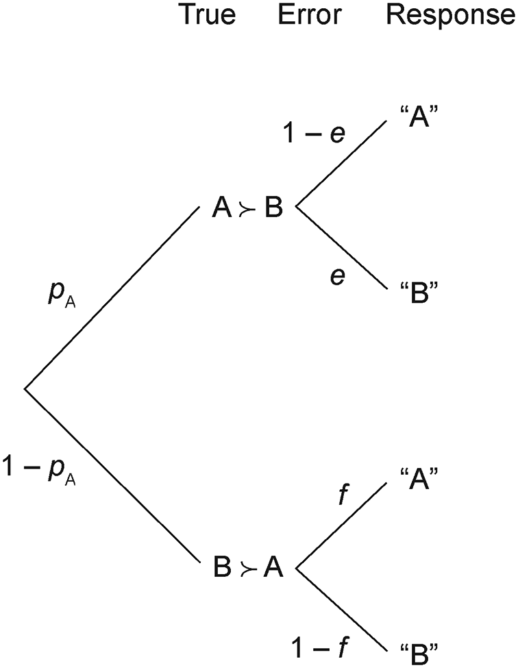
Let $p_{A}$
denote the probability that
$p_{A}$
denote the probability that $A \succ B$
in a certain population. The observed choice proportion,
$A \succ B$
in a certain population. The observed choice proportion, $P(A)$
, might be used to make inferences about a population choice probability,
$P(A)$
, might be used to make inferences about a population choice probability, $p(A)$
, but the question is, can we estimate the true preference probability,
$p(A)$
, but the question is, can we estimate the true preference probability, $p_{A}$
, from the observed choice proportion or inferred choice probability? No, because the choice probability is given as follows:
$p_{A}$
, from the observed choice proportion or inferred choice probability? No, because the choice probability is given as follows:
 $$ \begin{align} p(A) = p_{A}(1-e) + (1-p_{A)}f, \end{align} $$
so from $p(A)$
we cannot estimate
$p(A)$
we cannot estimate $p_{A}$
, unless we know or can estimate e and f.Footnote
2
$p_{A}$
, unless we know or can estimate e and f.Footnote
2
If someone were to assume that $p_{A}=1$
(e.g., that dominance is always satisfied), then the observation of 25% violations would indicate that
$p_{A}=1$
(e.g., that dominance is always satisfied), then the observation of 25% violations would indicate that $e=0.25$
; alternatively, another person who assumed that
$e=0.25$
; alternatively, another person who assumed that $e=f=0$
might conclude that there are 25% true violations. However, these arbitrary conclusions might be refuted by empirical evidence, if a better experiment (with replications) had been done.
$e=f=0$
might conclude that there are 25% true violations. However, these arbitrary conclusions might be refuted by empirical evidence, if a better experiment (with replications) had been done.
1.5. TE model with replications
Suppose that the same choice problem is presented twice to the same participants in the same brief session, with both presentations suitably separated and embedded among a number of other filler trials. There are 4 possible response patterns: a person might choose A both times (AA), B both times (BB), switch from A to B (AB), or switch from B to A (BA).
Table 1 contains hypothetical data for 100 participants who responded twice to the same choice problem. The marginals show that 75% chose A in either replicate, but 20% switched responses between replications. Since there are 100 participants, these values can be interpreted as percentages.
Hypothetical data for a replicated choice problem

Note: There are 75% responses for A in either replicate and 20% reversals between replicates.
Table 2 shows the theoretical probabilities of these 4 response patterns, $p(AA), p(AB), p(BA)$
, and
$p(AA), p(AB), p(BA)$
, and $p(BB)$
according to the TE model of Figure 2, assuming that true preferences are the same and errors on 2 replications have equal probability and are independent of each other. Table 2 shows that the probabilities of the 2 types of reversal are implied to be equal to each other,
$p(BB)$
according to the TE model of Figure 2, assuming that true preferences are the same and errors on 2 replications have equal probability and are independent of each other. Table 2 shows that the probabilities of the 2 types of reversal are implied to be equal to each other, $p(AB)=p(BA)$
, which can be used to test these assumptions.
$p(AB)=p(BA)$
, which can be used to test these assumptions.
TE4 analysis of replication of a single choice problem

Note: $p(A)=p_{A}(1-e) + (1-p_{A})(f)$
.
$p(A)=p_{A}(1-e) + (1-p_{A})(f)$
.
There are 3 parameters in the model, $p_A, e$
, and f, and there are 3 degrees of freedom in the data of Table 1. The data of this design constrain the parameters, but the constraints do not impose a unique solution. To illustrate these partial constraints, Figure 3 shows the fit of the TE model (Figure 2) to Table 1 for fixed values of p. For each value of p, error rates are selected to minimize G, which is defined as follows:
$p_A, e$
, and f, and there are 3 degrees of freedom in the data of Table 1. The data of this design constrain the parameters, but the constraints do not impose a unique solution. To illustrate these partial constraints, Figure 3 shows the fit of the TE model (Figure 2) to Table 1 for fixed values of p. For each value of p, error rates are selected to minimize G, which is defined as follows:
 $$ \begin{align} G=-2\sum O_iln(O_i/E_i), \end{align} $$
where $O_i$
and
$O_i$
and $E_i$
are the observed and ‘expected’ (fitted) frequencies of the 4 response patterns. In this case, the
$E_i$
are the observed and ‘expected’ (fitted) frequencies of the 4 response patterns. In this case, the $O_i$
are the entries of Table 1 and the
$O_i$
are the entries of Table 1 and the $E_i$
are the corresponding frequencies implied by Table 2; e.g., the ‘expected’ frequency of AA responses is
$E_i$
are the corresponding frequencies implied by Table 2; e.g., the ‘expected’ frequency of AA responses is $np(AA)$
from Table 2, where
$np(AA)$
from Table 2, where $n=100$
. Minimizing G (aka
$n=100$
. Minimizing G (aka $G^2$
) is equivalent to finding a maximum likelihood solution.
$G^2$
) is equivalent to finding a maximum likelihood solution.
Fit of true-and-error models as a function of the parameter, $p_A$
, the probability that
$p_A$
, the probability that $A \succ B$
. Solid line shows the fit of the 3-parameter model of Figure 2 (TE4), and the dashed line shows the fit of the 2-parameter model with
$A \succ B$
. Solid line shows the fit of the 3-parameter model of Figure 2 (TE4), and the dashed line shows the fit of the 2-parameter model with $e=f$
(TE2).
$e=f$
(TE2).

The solid curve in Figure 3 plots the best-fit value of G as a function of $p_A$
. The model fits Table 1 perfectly (
$p_A$
. The model fits Table 1 perfectly ( $G=0$
) for a range of values, about
$G=0$
) for a range of values, about $0.65<p_A<0.85$
, where e and f trade off from
$0.65<p_A<0.85$
, where e and f trade off from $e=0.03$
and
$e=0.03$
and $f=0.35$
at
$f=0.35$
at $p_A=0.65$
to
$p_A=0.65$
to $e=0.10$
and
$e=0.10$
and $f=0.16$
at
$f=0.16$
at $p_A=0.80$
to achieve the perfect fit.
$p_A=0.80$
to achieve the perfect fit.
Although we cannot identify a unique best-fitting $p_A, e$
, and
$p_A, e$
, and $f,$
we can reject the model if we assumed that
$f,$
we can reject the model if we assumed that $p_A =1$
, as shown by the large G value in Figure 3. (The critical values of
$p_A =1$
, as shown by the large G value in Figure 3. (The critical values of $\chi ^2(1)$
and
$\chi ^2(1)$
and $\chi ^2(2)$
are 6.34 and 9.21 with
$\chi ^2(2)$
are 6.34 and 9.21 with $\alpha = 0.01$
.) That is, even though the 3-parameter model exhausted the df in the data, it still imposes constraints that allow one to test specific hypotheses about certain specific values of
$\alpha = 0.01$
.) That is, even though the 3-parameter model exhausted the df in the data, it still imposes constraints that allow one to test specific hypotheses about certain specific values of $p_A$
.Footnote
3
The assumption that
$p_A$
.Footnote
3
The assumption that $p_A=1$
corresponds to the null hypothesis that dominance is always satisfied in a choice problem such as illustrated in Figure 1.
$p_A=1$
corresponds to the null hypothesis that dominance is always satisfied in a choice problem such as illustrated in Figure 1.
Furthermore, if we can assume that $e=f$
, then the model is fully identified and testable; that is, we can estimate both
$e=f$
, then the model is fully identified and testable; that is, we can estimate both $p_A$
and e from the data, and we can test the model without specifying
$p_A$
and e from the data, and we can test the model without specifying $p_A$
. This 2-parameter model, in which each choice problem is allowed to have a different true probability and a different error rate, is termed the TE2 model in Birnbaum and Quispe-Torreblanca (Reference Birnbaum and Quispe-Torreblanca2018), and the more complex model of Figure 2, with 2 error terms for each choice problem, is known as TE4.
$p_A$
. This 2-parameter model, in which each choice problem is allowed to have a different true probability and a different error rate, is termed the TE2 model in Birnbaum and Quispe-Torreblanca (Reference Birnbaum and Quispe-Torreblanca2018), and the more complex model of Figure 2, with 2 error terms for each choice problem, is known as TE4.
With $e=f$
, it follows from the equations (Table 2) that the sum of response reversals between replicates is a quadratic function of e, as follows:
$e=f$
, it follows from the equations (Table 2) that the sum of response reversals between replicates is a quadratic function of e, as follows:
 $$ \begin{align} p(AB)+p(BA)=2(1-e)e. \end{align} $$
Because there are 20% reversals between replications in Table 1, $e=0.113$
.Footnote
4
Once e is determined,
$e=0.113$
.Footnote
4
Once e is determined, $p_A$
can be computed from the estimated binary choice proportion, substituted for
$p_A$
can be computed from the estimated binary choice proportion, substituted for $p(A)$
in the expression,
$p(A)$
in the expression, $p(A) = p_A(1-e)+ (1-p_A)e$
. For Table 1,
$p(A) = p_A(1-e)+ (1-p_A)e$
. For Table 1, $0.75= p_A(1-0.113) + (1-p_A)(0.113)$
, which implies
$0.75= p_A(1-0.113) + (1-p_A)(0.113)$
, which implies $p_A=$
0.823. In practice, one solves for
$p_A=$
0.823. In practice, one solves for $p_A$
and e to fit all the data (e.g., all values in Table 1) minimizing G. Because this TE2 model uses only 2 parameters, there remains 1 df to test the model.
$p_A$
and e to fit all the data (e.g., all values in Table 1) minimizing G. Because this TE2 model uses only 2 parameters, there remains 1 df to test the model.
The dashed line in Figure 3 shows the index of fit of TE2 to Table 1 as a function of $p_A$
; unlike TE4 which has multiple solutions, TE2 has a unique minimum at
$p_A$
; unlike TE4 which has multiple solutions, TE2 has a unique minimum at $p_A=0.82$
. According to TE2, values of
$p_A=0.82$
. According to TE2, values of $p_A$
in the range from about 0.75 to 0.90 are considered statistically acceptable, but values outside that range are not, including
$p_A$
in the range from about 0.75 to 0.90 are considered statistically acceptable, but values outside that range are not, including $p_A=1$
.Footnote
5
Although both TE2 and TE4 achieve a perfect fit to this example, that need not be the case. Both TE2 and TE4 would be rejected (binomial
$p_A=1$
.Footnote
5
Although both TE2 and TE4 achieve a perfect fit to this example, that need not be the case. Both TE2 and TE4 would be rejected (binomial $p < 0.01$
) if the entries of Table 1 were instead 65, 5, 20, and 10, for example, because both models imply that
$p < 0.01$
) if the entries of Table 1 were instead 65, 5, 20, and 10, for example, because both models imply that $p_{AB}=p_{BA}$
.
$p_{AB}=p_{BA}$
.
In sum, if we replicate a single choice problem, we can use either TE4 or TE2 to test whether violations of a property like dominance are ‘real’ (systematic), or instead might be due to random error. Furthermore, if we can assume that $e=f$
, we can uniquely estimate the incidence of true violations.
$e=f$
, we can uniquely estimate the incidence of true violations.
1.6. True-and-error model of transitivity
The issue of transitivity is important because descriptive theories disagree about whether transitivity of preference can be systematically violated. Some important papers reviewing transitivity in terms of empirical results, theory, or error analysis include Bhatia and Loomes (Reference Bhatia and Loomes2017), Birnbaum (Reference Birnbaum2023a), Budescu and Weiss (Reference Budescu and Weiss1987), Cavagnaro and Davis-Stober (Reference Cavagnaro and Davis-Stober2014), Fishburn (Reference Fishburn1991), Gonzalez-Vallejo (Reference Gonzalez-Vallejo2002), Iverson and Falmagne (Reference Iverson and Falmagne1985), Leland (Reference Leland1998), Loomes and Sugden (Reference Loomes and Sugden1982), Luce (Reference Luce2000), Morrison (Reference Morrison1963), Müller-Trede et al. (Reference Müller-Trede, Sher and McKenzie2015), Ranyard et al. (Reference Ranyard, Montgomery, Konstantinidis and Taylor2020), Regenwetter et al. (Reference Regenwetter, Dana and Davis-Stober2011), Rieskamp et al. (Reference Rieskamp, Busemeyer and Mellers2006), Sopher and Gigliotti (Reference Sopher and Gigliotti1993), and Tversky (Reference Tversky1969).
Much of the empirical research on the descriptive accuracy of transitivity has been highly controversial because that research has not used appropriate experimental designs coupled with appropriate quantitative analyses that can actually diagnose whether transitivity violations are real or due to error (Birnbaum, Reference Birnbaum2023a; Birnbaum and Wan, Reference Birnbaum and Wan2020). Birnbaum (Reference Birnbaum2023a) and Birnbaum and Wan (Reference Birnbaum and Wan2020) noted that quantitative methods used in the past can easily conclude that data generated by an intransitive process are ‘transitive’ or vice versa. Fortunately, TE models can be applied to separate the issue of systematic violation of transitivity from that of error, but one needs to do a proper experiment with replications to apply these methods.
Methods for analyzing transitivity via TE models have been presented in Birnbaum (Reference Birnbaum2020, Reference Birnbaum2023a), Birnbaum et al. (Reference Birnbaum, Navarro-Martinez, Ungemach, Stewart and Quispe-Torreblanca2016), Birnbaum and Bahra (Reference Birnbaum and Bahra2012a), Birnbaum and Diecidue (Reference Birnbaum and Diecidue2015), Birnbaum and Gutierrez (Reference Birnbaum and Gutierrez2007), Birnbaum and Schmidt (Reference Birnbaum and Schmidt2008), and Birnbaum and Wan (Reference Birnbaum and Wan2020). In these earlier papers, however, it had been assumed that each choice problem has a different error rate, but it was assumed $e_i=f_i$
.
$e_i=f_i$
.
In this article, the more general model of Figure 2 where e need not equal f will be employed. It has not yet been ruled out that this more complex error specification might allow transitive models to be accepted that would have been rejected under the simpler models, despite simulations in Birnbaum and Quan (Reference Birnbaum and Quan2020) showing that conclusions regarding transitivity appear to be robust with respect to the error specifications in TE models.
Consider a test of transitivity with three choice problems, XY, YZ, and ZX. If we code 1 to represent choice of the first listed option and 2 for choice of the second, there are 8 possible response patterns: 111, 112, 121, $\dots $
, 222. For example, 111 is the intransitive pattern of choosing X over Y, Y over Z, and Z over X; 222 is the opposite intransitive pattern, and the other 6 patterns are transitive. However, if we present each choice problem twice (replicate), there are 64 possible response patterns for the 6 choice problems.Footnote
6
$\dots $
, 222. For example, 111 is the intransitive pattern of choosing X over Y, Y over Z, and Z over X; 222 is the opposite intransitive pattern, and the other 6 patterns are transitive. However, if we present each choice problem twice (replicate), there are 64 possible response patterns for the 6 choice problems.Footnote
6
The observed frequencies of the 64 response patterns can be fit to the TE model of Figure 2. In this case, there are 8 parameters representing the 8 possible true preference patterns, $p_{111}, p_{112}, p_{121}, p_{122}, p_{211}, p_{212}, p_{221},$
and
$p_{111}, p_{112}, p_{121}, p_{122}, p_{211}, p_{212}, p_{221},$
and $p_{222}$
, and 6 error rates,
$p_{222}$
, and 6 error rates, $e_1, e_2, e_3, f_1, f_2,$
and
$e_1, e_2, e_3, f_1, f_2,$
and $f_3$
for the 3 choice problems. Since the 8 true preference pattern probabilities sum to 1, they consume 7 df, so the parameters use 7 + 6 = 13 df. The 64 cell frequencies have 63 df because their probabilities also sum to 1, so there are
$f_3$
for the 3 choice problems. Since the 8 true preference pattern probabilities sum to 1, they consume 7 df, so the parameters use 7 + 6 = 13 df. The 64 cell frequencies have 63 df because their probabilities also sum to 1, so there are $63-13=50$
df remaining to test the model.
$63-13=50$
df remaining to test the model.
The ‘expected’ (i.e., ‘fitted’ or ‘predicted’) frequency for the response pattern 212, on the first replicate and the pattern 211 on the second (denoted 212, 211), for example, is given as follows:
 $$ \begin{align} E_{212,211} & = n[p_{111}(e_1)^2(1-e_2)^2(e_3)(1 - e_3) \nonumber\\&\quad + p_{112}(e_1)^2(1-e_2)^2(1-f_3)(f_3)\nonumber\\&\quad + p_{121}(e_1)^2(f_2)^2(e_3)(1-e_3)\nonumber\\&\quad + p_{122}(e_1)^2(f_2)^2(1-f_3)(f_3)\\&\quad + p_{211}(1-f_1)^2(1-e_2)^2(e_3)(1-e_3)\nonumber\\&\quad + p_{212}(1-f_1)^2(1-e_2)^2(1-f_3)(f_3)\nonumber\\&\quad + p_{221}(1-f_1)^2(f_2)^2(e_3)(1-e_3)\nonumber\\&\quad + p_{222}(1-f_1)^2(f_2)^2(1-f_3)(f_3)],\nonumber \end{align} $$
where $E_{212,211}$
is the ‘expected’ (‘fitted’) frequency (count) that people will respond with the 212 and 211 response patterns in the first and second replications of the session. Note that if a person has the true preference pattern of 111, then she or he would have to make error
$E_{212,211}$
is the ‘expected’ (‘fitted’) frequency (count) that people will respond with the 212 and 211 response patterns in the first and second replications of the session. Note that if a person has the true preference pattern of 111, then she or he would have to make error $e_1$
twice on the first choice problem, make no error on the 2 presentations of the second problem, and make 1 error and 1 correct on the third choice problem. If the true pattern were 212, then this response pattern could occur if the person made only 1 error in the second replicate on the third choice problem. Note that when the true preference is assumed to be 212, the first and third choice problems involve error terms,
$e_1$
twice on the first choice problem, make no error on the 2 presentations of the second problem, and make 1 error and 1 correct on the third choice problem. If the true pattern were 212, then this response pattern could occur if the person made only 1 error in the second replicate on the third choice problem. Note that when the true preference is assumed to be 212, the first and third choice problems involve error terms, $f_1$
and
$f_1$
and $f_3$
. Each ‘expected’ frequency is simply n times the theoretical probability, where n is the total count of responses. There are 64 equations (including this one) for the 64 possible response patterns.
$f_3$
. Each ‘expected’ frequency is simply n times the theoretical probability, where n is the total count of responses. There are 64 equations (including this one) for the 64 possible response patterns.
The TE2 model (in which $e_i=f_i$
) is a special case of this TE4 model; TE2 uses 3 fewer parameters, so these models can be compared by computing the difference in fit between the 2 models,
$e_i=f_i$
) is a special case of this TE4 model; TE2 uses 3 fewer parameters, so these models can be compared by computing the difference in fit between the 2 models, $G(3)=G(53)-G(50)$
. In theory, the difference asymptotically approaches a chi-squared distribution with 3 df as n increases.
$G(3)=G(53)-G(50)$
. In theory, the difference asymptotically approaches a chi-squared distribution with 3 df as n increases.
Within either TE2 or TE4, transitivity is a special case in which $p_{111} = p_{222} = 0$
. The differences in fit testing transitivity each have 2 df.
$p_{111} = p_{222} = 0$
. The differences in fit testing transitivity each have 2 df.
The nesting relationships among these 4 models are the same as in Birnbaum (Reference Birnbaum2019, Figure 2), except where ‘transitivity’ is substituted for ‘EU’. In particular, it is possible that data that would refute transitivity with TE2 might be compatible with transitivity under TE4.
A spreadsheet employing Excel’s Solver to fit either TE2 or TE4 to a replicated test of transitivity is included in the Supplementary Material to this article.Footnote 7
2. Method
Participants made choices between pairs of gambles, each of which had 3 equally likely prizes. The prize of a gamble is determined by the color of marble drawn blindly and randomly from a single urn containing an equal number of red, white, and blue marbles.
Choices were displayed as in Figure 1, where rows represented the 2 choice alternatives, and columns (colored red, white, and blue) represented the 3 possible outcomes. Numerical entries indicated money prizes to be won if a marble drawn randomly from an urn was red, white, or blue. The urn contained 33 red, 33 white, and 33 blue marbles. These displays are like those in Birnbaum (Reference Birnbaum2023a) and Birnbaum and Diecidue (Reference Birnbaum and Diecidue2015).
2.1. Instructions and materials
Instructions, and one block of trials can be viewed at the following URL: https://konstanzworkshop.neocities.org/CSUF22/MPW_01a.
Stimulus displays and Web forms were constructed and randomized using a free program, available at the following URL: http://psych.fullerton.edu/mbirnbaum/programs/ChoiceTableColorWiz2.htm.
2.2. Transitivity design
There were 4 triples of gambles, which showed the highest incidence of intransitive behavior in Butler and Pogrebna (Reference Butler and Pogrebna2018) and used in Birnbaum (Reference Birnbaum2023a). The amounts (in dollars, instead of pounds) are as follows:
Triple 1: $X=(12, 12, 2)$
;
$X=(12, 12, 2)$
; $Y=(8, 8, 8)$
;
$Y=(8, 8, 8)$
; $Z=(20, 4, 4)$
.
$Z=(20, 4, 4)$
.
Triple 2: $X=(15, 15, 3)$
;
$X=(15, 15, 3)$
; $Y=(10, 10, 10)$
;
$Y=(10, 10, 10)$
; $Z=(27, 5, 5)$
.
$Z=(27, 5, 5)$
.
Triple 3: $X=(9, 9, 3)$
;
$X=(9, 9, 3)$
; $Y=(6, 6, 6)$
;
$Y=(6, 6, 6)$
; $Z=(16, 4, 4)$
.
$Z=(16, 4, 4)$
.
Triple 4: $X=(14, 14, 2)$
;
$X=(14, 14, 2)$
; $Y=(8, 8, 8)$
;
$Y=(8, 8, 8)$
; $Z=(21, 6, 6)$
.
$Z=(21, 6, 6)$
.
Note that in all 4 triples, Y is always a ‘sure thing’ with the smallest EV; Z always has the highest EV and greatest range; and X is intermediate in both EV and range. The MPW model favors X over Y, Y over Z, and Z over X in all 4 triples.
There are 6 choice problems for each triple as follows: XY, YZ, and ZX; and YX, ZY, and XZ, where XY and YX denote the same choice problem, except X is displayed in the first or second position. With 4 triples and 6 choice problems per triple, there are 24 experimental choice problems testing transitivity in each block.
2.3. Dominance design
Four tests of transparent dominance were included in each block: D1: $T=(10, 9, 8)$
versus
$T=(10, 9, 8)$
versus $U=(8, 8, 8)$
; D2:
$U=(8, 8, 8)$
; D2: $V=(10, 10, 7)$
versus
$V=(10, 10, 7)$
versus $W=(12, 12, 8)$
; D3:
$W=(12, 12, 8)$
; D3: $A=(4, 4, 2)$
versus
$A=(4, 4, 2)$
versus $B=(8, 8, 8)$
, D4:
$B=(8, 8, 8)$
, D4: $C=(8, 8, 8)$
versus
$C=(8, 8, 8)$
versus $D=(5, 5, 2)$
. Note that in Choices D1 and D2, the wider range gamble is dominant, whereas in D3 and D4, the wider range gamble is dominated.
$D=(5, 5, 2)$
. Note that in Choices D1 and D2, the wider range gamble is dominant, whereas in D3 and D4, the wider range gamble is dominated.
2.4. Procedure
Each block consisted of 28 randomly ordered trials (choice problems) intermixed from both subdesigns.
When a block was completed, the participant pushed a button to submit the responses, and then pressed another button to load the materials for the second block. Participants participated via the WWW, and worked at their own paces.
Instructions stated that 3 participants would be selected at random to receive the prize of one of their chosen gambles, so they should choose wisely. Procedures for determining prizes were similar to those in Birnbaum and Diecidue (Reference Birnbaum and Diecidue2015, Experiment 6), except contestants were not present and prizes were sent as cash in the mail.
2.5. Participants
The participants were 260 undergraduates who completed 2 blocks (ages 18–38, with 76% $\le 20$
years; 24% males, 72% females, and 3% not responding) who participated in partial fulfillment of an assignment in Introductory Psychology.
$\le 20$
years; 24% males, 72% females, and 3% not responding) who participated in partial fulfillment of an assignment in Introductory Psychology.
Because each of the 12 choice problems testing transitivity was replicated twice in each block with display position (First or Second) counterbalanced, the number of consistent responses within a block could range from 0 to 12; a person who mindlessly pushed the same button would show zero consistency, and a person who pushed buttons randomly would be expected to have a score of 6 (50% agreement). There were 40 participants who had low consistency in at least one block whose data were analyzed separately, leaving 220 participants with mean consistency of 84% within-block agreement between replicates of the 12 choices testing transitivity.
3. Results
3.1. Tests of dominance
The first 4 rows of Table 3 show the numbers of participants (out of 220) who had each response pattern in 2 replications of the 2 tests of dominance. For example, the first row (for choice problem D1) shows that 145 participants (out of 220) satisfied dominance on both replications (AA); 22, 19, and 34 violated it only on the second replication (AB), only on the first (BA), or violated dominance on both replications (BB), respectively. There were thus $22+19+(2)(34)= 109$
total violations out of 440 choice responses, or 25%, which is shown in the column labeled ‘Resp viol’, representing response violations.
$22+19+(2)(34)= 109$
total violations out of 440 choice responses, or 25%, which is shown in the column labeled ‘Resp viol’, representing response violations.
Response patterns in replicated tests of dominance and TE analysis

Note: Critical $\chi ^2(1)$
= 6.64 and
$\chi ^2(1)$
= 6.64 and $\chi ^2(2)=9.21$
for
$\chi ^2(2)=9.21$
for $\alpha = 0.01$
.
$\alpha = 0.01$
.
The column in Table 3 labeled ‘ $\chi ^2(1) Indep$
’ is the standard chi-squared test of response independence, which is the assumption that the probability of a conjunction of responses is the product of the marginal probabilities of those responses; that is,
$\chi ^2(1) Indep$
’ is the standard chi-squared test of response independence, which is the assumption that the probability of a conjunction of responses is the product of the marginal probabilities of those responses; that is, $p(AA)=p(A)p(A)$
. Because the critical value of
$p(AA)=p(A)p(A)$
. Because the critical value of $\chi ^2(1)$
is 6.34 with
$\chi ^2(1)$
is 6.34 with $\alpha = 0.01$
, we can reject the hypothesis that responses are independent in the first 4 rows of Table 3.
$\alpha = 0.01$
, we can reject the hypothesis that responses are independent in the first 4 rows of Table 3.
Independence is implied to be violated by the TE models, except in special cases, such as when $p_A=1$
, which implies
$p_A=1$
, which implies $p(A) = 1-e$
, so
$p(A) = 1-e$
, so $p(AA)=(1-e)(1-e)=p(A)p(A)$
. Note also that if
$p(AA)=(1-e)(1-e)=p(A)p(A)$
. Note also that if $p_A=1$
,
$p_A=1$
, $p(BB)=e^2 < p(AB)=p(BA)=e(1-e)$
; that is, the probability of a repeated violation should be less than that of a reversal of preference between violation and satisfaction of dominance. The large
$p(BB)=e^2 < p(AB)=p(BA)=e(1-e)$
; that is, the probability of a repeated violation should be less than that of a reversal of preference between violation and satisfaction of dominance. The large $\chi ^2$
for violation of independence occur when the frequency of BB exceeds that of AB and BA, indicating
$\chi ^2$
for violation of independence occur when the frequency of BB exceeds that of AB and BA, indicating $p_A<1$
.
$p_A<1$
.
The next column in Table 3, labeled ‘ $G(1) TE2$
’, displays the G tests of the TE2 model (
$G(1) TE2$
’, displays the G tests of the TE2 model ( $e=f$
), which has 1 df and is asymptotically chi-squared distributed. As can be seen in the table, all of these
$e=f$
), which has 1 df and is asymptotically chi-squared distributed. As can be seen in the table, all of these $G(1)$
values are much less than corresponding tests of response independence and all show good fits to the data, even though the number of parameters estimated (and thus the df) is the same as for the tests of independence. The best-fit parameter estimates of the TE2 model are shown in the next columns, labeled ‘
$G(1)$
values are much less than corresponding tests of response independence and all show good fits to the data, even though the number of parameters estimated (and thus the df) is the same as for the tests of independence. The best-fit parameter estimates of the TE2 model are shown in the next columns, labeled ‘ $1-p_A$
’ and ‘e’, representing the probability of systematic violation of dominance and of random error, respectively.
$1-p_A$
’ and ‘e’, representing the probability of systematic violation of dominance and of random error, respectively.
The next to last column in Table 3 is a $G(2)$
test of the TE model with the assumption that
$G(2)$
test of the TE model with the assumption that $p_A=1$
; this test is the same in either TE2 or TE4 because when
$p_A=1$
; this test is the same in either TE2 or TE4 because when $p_A=1$
, the parameter f drops out of the equations. The last column in Table 3, labeled ‘DIFF’, shows the differences,
$p_A=1$
, the parameter f drops out of the equations. The last column in Table 3, labeled ‘DIFF’, shows the differences, $G(2)-G(1)$
, which test if
$G(2)-G(1)$
, which test if $p_A=1$
. These indicate that the violations of transparent dominance, estimated to range from 4% to 18% in the 4 choice problems of the first 4 rows, are significantly greater than 0, because all 4 values well exceed the critical value of 6.64 with
$p_A=1$
. These indicate that the violations of transparent dominance, estimated to range from 4% to 18% in the 4 choice problems of the first 4 rows, are significantly greater than 0, because all 4 values well exceed the critical value of 6.64 with $\alpha = 0.01$
.
$\alpha = 0.01$
.
Participants were subdivided according to their modal response patterns in the tests of transitivity. There were 89 participants who most often preferred ‘sure things’ when presented in these non-dominated choice problems, 77 of whom most often preferred the lower range option in any non-dominated choice. That left 131 who did not show one of these modal response patterns.
These two subgroups of data were then analyzed separately, shown by the next 2 groups of 4 rows each. For the group of 89 who prefer ‘sure things’, the estimated true rates of violation were 0.45 and 0.28 for D1 and D2, corrected for error, which are similar to the findings in Birnbaum (Reference Birnbaum2023a) and seem ‘large’ for tests of transparent dominance. The estimated violation rates for the other 131 participants are only around 0.03 for the 4 problems. These data for D1 and D2 therefore are consistent with Birnbaum’s (Reference Birnbaum2023a) findings that relatively large rates of violation of transparent dominance can be observed, and that these high violations are mainly found in people who appear to favor ‘safer’ (i.e., lower-ranged) gambles in non-dominated choice problems.Footnote 8
Among the 89 participants who favor ‘safer’ gambles in non-dominated choices, the rates of violation of dominance for D3 and D4 are lower, 0.12 and 0.06, respectively, compared to 0.45 and 0.28 for D1 and D2. Although D3 and D4 have lower rates, as hypothesized, 12% violations for D3 still seems surprisingly high for this risk-averse group, since choosing the ‘safer’ alternative in D3 or D4 would have satisfied dominance.Footnote 9
For the group of 131, the rates of violation for D3 and D4 are low in all tests (3% or lower) and the discrepancy (comparing D3 and D4 to D1 and D2) is not as pronounced as for the group of 89.
3.2. Tests of transitivity
Table 4 shows a cross-tabulation of response patterns in 2 replicates, aggregated over participants, choice triples, and blocks. Each response pattern represents 6 responses (3 choice problems with 2 replications). For example, the entry of 15 in row 111 and column 111 indicates that there were 15 occasions (out of 1,760) in which a participant chose X over Y, Y over Z, and Z over X on both replicates of a choice triple in a block. This response pattern, 111, is the intransitive cycle implied by the MPW model (for all 4 triples).
Crosstabulation. Frequencies of response patterns in first (rows) and second (columns) replications, aggregated over participants, choice triples, and sessions

Note: Total n = 1,760 = 220 Participants by 4 Triples by 2 Sessions, each based on 6 responses (3 choices problems by 2 repetitions) per triple. The pattern 111 is the intransitive pattern predicted by most probable winner rule.
The diagonal entries in Table 4 represent frequencies of repeating the same response pattern in both replicates, and the off-diagonal entries are cases where at least 1 of the 3 choice problems produced opposite responses in the 2 replicates. The row and column sums (totals) represent frequencies of response patterns in the first and second replications, respectively.
The last row at the bottom of Table 4, labeled ‘Mode’, shows the number of individuals who showed each modal response pattern, aggregated over triples, replicates, and blocks.
The most frequently observed and repeated pattern is 212, which is the transitive pattern implied by the TAX model with its ‘prior’ parameters. Those parameters were roughly estimated in 1996 (described in Birnbaum and Chavez, Reference Birnbaum and Chavez1997) and used to make predictions for new studies for the next quarter century (Birnbaum, Reference Birnbaum and Marley1997, Reference Birnbaum2008, Reference Birnbaum2020, Reference Birnbaum2023a). The 212 pattern was also the most frequently observed modal pattern by individuals. This pattern was also the pattern estimated to be most frequent in each Triple when separately analyzed, and was most frequent in previous studies by Butler and Pogrebna (Reference Butler and Pogrebna2018) and by Birnbaum (Reference Birnbaum2023a). It is also the response pattern consistent with preference for ‘safer’ (lower range) gambles, despite the lower EV.
Table 4 shows that second most frequently repeated pattern was the transitive pattern, 121, which is the response pattern implied if people chose the gamble with the higher expected value (EV). Other frequently observed patterns include 112, consistent with selecting the gamble with the higher median and 122, which could be compatible with a ‘sufficing’ interpretation (Birnbaum, Reference Birnbaum2020, Reference Birnbaum2023a). The least frequent response patterns are the 2 intransitive patterns, 111 and 222. Although 8 of 220 participants showed one of these intransitive patterns as their most frequent response pattern (3.6%), only 3 of these 8 showed one of these patterns more often than 5 times out of 16 possible (4 triples by 2 blocks by 2 replicates).
Table 5 shows the fit of TE models to the data in Table 4. The 64 entries in Table 4 have 63 df. The TE4 model with all parameters free uses 8 estimates of probabilities of the preference patterns ( $p_{111}, p_{112}, \dots , p_{222}$
) and 6 error terms (
$p_{111}, p_{112}, \dots , p_{222}$
) and 6 error terms ( $e_1, e_2, e_3, f_1, f_2, f_3$
), which consume 13 df, leaving 50 df to test the model. The TE2 model is a special case of TE4 in which
$e_1, e_2, e_3, f_1, f_2, f_3$
), which consume 13 df, leaving 50 df to test the model. The TE2 model is a special case of TE4 in which $e_i=f_i$
, so it has 3 additional df. Within each version of the TE model, the transitive special cases assume
$e_i=f_i$
, so it has 3 additional df. Within each version of the TE model, the transitive special cases assume $p_{111}=p_{222}=0$
, and thus leave an additional 2 df. Assuming large n and assuming that responses across sessions by the same person were independent, the G should follow a chi-squared distribution with 50–55 df for these 4 models.
$p_{111}=p_{222}=0$
, and thus leave an additional 2 df. Assuming large n and assuming that responses across sessions by the same person were independent, the G should follow a chi-squared distribution with 50–55 df for these 4 models.
Indices of fit for four models of Table 4

Note: ‘Trans’ indicates transitive; ‘Free’ includes all transitive and intransitive patterns.
The difference in fit between TE2 and TE4 has 3 df, and the difference between each TE model and its transitive special case has 2 df. However, the G tests are likely inflated by small frequencies in many cells and the fact that each participant served in 2 blocks and 4 choice triples; therefore, some caution should be exercised when comparing these G values against the theoretical chi-squared distribution. If we take these tests in Table 5 at face value, caveats notwithstanding, both tests of transitivity far exceed the critical $\chi ^2(2)=9.2$
for
$\chi ^2(2)=9.2$
for $\alpha =0.01$
, indicating that transitivity can be rejected, whereas the test of TE4 against TE2 exceeds the critical
$\alpha =0.01$
, indicating that transitivity can be rejected, whereas the test of TE4 against TE2 exceeds the critical $\chi ^2(3)=11.3$
with
$\chi ^2(3)=11.3$
with $\alpha = 0.01$
in the transitive case, but it falls just short of the critical value for the TE model with all parameters free. Examining the predictions of TE4 and TE2 against the empirical values in Table 4, the improvement of TE4 over TE2 is not impressive. However, even if TE4 does not provide a substantially better fit to data compared to TE2, it is important to evaluate TE4 for both transitive and intransitive cases, because of its theoretical potential to yield a transitive solution that might be compatible with data. In this case, though, it did not change the conclusions regarding transitivity.
$\alpha = 0.01$
in the transitive case, but it falls just short of the critical value for the TE model with all parameters free. Examining the predictions of TE4 and TE2 against the empirical values in Table 4, the improvement of TE4 over TE2 is not impressive. However, even if TE4 does not provide a substantially better fit to data compared to TE2, it is important to evaluate TE4 for both transitive and intransitive cases, because of its theoretical potential to yield a transitive solution that might be compatible with data. In this case, though, it did not change the conclusions regarding transitivity.
Table 6 shows the best-fit parameters of 4 TE models fit to the data in Table 4. To save space in the table, estimated probabilities are displayed as percentages; for example, 09 indicates 0.09. According to either TE2 or TE4, the sum of probabilities of the 2 intransitive preference patterns is only 3%. Although the incidence of intransitive behavior appears minimal, it is statistically significant; even if we adopted the conservative procedure of dividing each G difference in Table 5 by 8 (4 triples by 2 blocks per participant), we can see that the G test would indicate ‘significant’ deviations from the transitive models, since the critical value of $\chi ^2(2)=5.99$
with
$\chi ^2(2)=5.99$
with $\alpha = 0.05$
. A further analysis of this statistical issue is presented for each block and each triple in the Appendix.
$\alpha = 0.05$
. A further analysis of this statistical issue is presented for each block and each triple in the Appendix.
Parameter estimates for true and error models fit to Table 4

Note: Values displayed as percentages, so 09 indicates 0.09. Parameters shown in parentheses are fixed or constrained.
Even if it is statistically significant, the estimate is only 3% intransitive behavior. For comparison, the data of Butler and Pogrebna (Reference Butler and Pogrebna2018) had 18% violations, averaged over 11 triples used in that study (44% violations in the 4 triples selected with the highest levels of violation in that study, which obviously includes capitalization on chance). Birnbaum (Reference Birnbaum2023a) found 14% violations for those same 4 selected triples in a study with 30 sessions. Thus, the finding here of only 3% is substantially lower than observed for the same triples in previous, similar studies.
The same analyses were conducted for each triple of choice problems separately. In all 4 triples, the estimate of intransitive preferences under either TE2 or TE4 was 4% or less. Triple 4 showed the largest evidence of intransitive preferences, with estimated 1% of 111 and 3% of 222 intransitive preference patterns. The $G(50)$
for the TE4 model was 54.01 with all parameters free, and it was 80.4, when it was assumed that
$G(50)$
for the TE4 model was 54.01 with all parameters free, and it was 80.4, when it was assumed that $p_{111}=p_{222}=0$
, yielding
$p_{111}=p_{222}=0$
, yielding $G(2)=26.4$
, more than double the critical value required for statistical significance (
$G(2)=26.4$
, more than double the critical value required for statistical significance ( $p<0.01)$
. The TE2 model fit nearly as well as TE4,
$p<0.01)$
. The TE2 model fit nearly as well as TE4, $G(53)=55.3$
, which is not significantly worse than the fit of TE4. The transitive special case of TE2 had
$G(53)=55.3$
, which is not significantly worse than the fit of TE4. The transitive special case of TE2 had $G(55)=82.62$
.
$G(55)=82.62$
.
Additional details of the separate analyses for each triple are included in the Appendix and Supplementary Material; overall, the results of separate analysis of the triples appear consistent with the conclusions that the transitive 212 pattern was most frequent for all triples, that intransitive behavior was probably ‘real’ but minimal, that the TE2 model fits almost as well as TE4. Consistent with simulations by Birnbaum and Quan (Reference Birnbaum and Quan2020), the choice of TE model for these real data did not appear to affect conclusions regarding transitivity.
The data for the 40 unreliable participants were analyzed separately. Aggregating over triples, as in Table 4, there were only 6 instances (out of 320 possible occasions) in which a participant repeated an intransitive response pattern in a block. The TE4 and TE2 models estimated the probability of intransitive response patterns to be 0.003 and 0.0, respectively, with 0.97 or more of the probability concentrated in 3 transitive response patterns, 121, 122, and 212 in both solutions. The estimated error rates ranged from 0.25 to 0.50 for TE4 and from 0.37 to 0.39 for TE2. Thus, although the error rates were higher for these participants, there was no evidence of systematic violation of transitivity in this group.
4. Discussion
The tests of transparent dominance corroborate 2 findings observed in Birnbaum (Reference Birnbaum2023a) and reveal a new result: first, violations of transparent dominance, while infrequent, are statistically significant when analyzed for all participants; second, violations of dominance are mainly found among people who systematically preferred the ‘safer’ gambles in other choice problems and are very rare for other participants; third, the new tests show that violations are much less frequent when the ‘safe’ gamble is dominant rather than when the ‘safe’ gamble is dominated by the ‘risky’ gamble.
4.1. Why violate transparent dominance?
I suspect that these violations of transparent dominance may be the result of the experimental design in which almost every trial paired a ‘safe’ gamble against a ‘riskier’ one with higher expected value. Brunswik (Reference Brunswik1956) theorized that humans adapt their behavior to the environment; in the environment of an experiment, stimulus designs will affect the behavior that the experiment is designed to explore. Brunswik thought that between-subjects designs totally isolate the participant from the variation and co-variation of the important variables. He found systematic factorial designs an improvement but thought that these must induce zero correlations among factors, and so he favored hybrid design, in which a factorial design is modified to remove unrepresentative combinations of variables. Ultimately, he argued against systematic design in favor of representative design, in which stimuli and situations are sampled from the environment to which generalization was desired.
Birnbaum (Reference Birnbaum, Restle, Shiffrin, Castellan, Lindman and Pisoni1975) reviewed several studies using systextual design, in which the context is systematically manipulated; these studies show that the direction of a main effect of a variable can even be reversed by systematically changing the correlation between that variable and the stimulus to be judged. Mellers et al. (Reference Mellers, Ordóñez and Birnbaum1992a) showed that by systematically changing the selection of stimuli presented in a study, one could change the rank order of judgments of a set of common stimuli (preference order), consistent with the theory that the experimental context caused a change in the model or process by which the information was combined.
Thus, it is not implausible that the Butler and Pogrebna (Reference Butler and Pogrebna2018) design, in which every choice fit the same recipe, may induce a decision strategy in some risk-averse participants to seek the low-range option without contrasting outcomes between gambles, a strategy that would lead them to violate dominance on trials in which the ‘safe’ gamble was dominated by the alternative.
Choosing gambles with lower range, without comparing consequences between gambles, would perhaps be an easy way to find ‘safe’ gambles in the Butler and Pogrebna design, but can induce people to violate dominance, if a choice problem is included in which the ‘safe’ gamble is dominated by the ‘risky’ gamble. This strategy for this experimental design would produce the 212 response pattern in tests of transitivity.
How would a person detect and satisfy dominance in a choice problem such as in Figure 1? If one compared the consequences on each branch (for each color of marble) of the gamble, one could detect dominance by counting the number of branches that are equal or favor one gamble over the other. Then choose the alternative with the greater number of winning branches. Ironically, such a strategy that can detect and satisfy dominance could also lead to violations of transitivity. If one chooses the gamble with the greater number of contrasts that favor one gamble over the other, one would violate transitivity in the design testing transitivity here with the response pattern, 111. With equally likely branches, this strategy is equivalent to the MPW model (aka, ‘majority rule’) that was used to design the studies of Birnbaum and Diecidue (Reference Birnbaum and Diecidue2015) and of Butler and Pogrebna (Reference Butler and Pogrebna2018).
4.2. Few violations of transitivity
Although Birnbaum (Reference Birnbaum2023a) and Butler and Pogrebna (Reference Butler and Pogrebna2018) found evidence of 18% and 14% systematic violations of transitivity, the present data contained only very small incidence of intransitive behavior, about 3%, including about 1% of the MPW type and 2% of the opposite (‘regret’) type. These estimates were similar whether the TE2 model (used in previous analyses) or the TE4 model was used to provide these estimates while correcting for error.
Although the TE4 model fits the data only slightly better than TE2, the main reason to use this analysis is to find out whether or not the conclusions regarding violations of transitivity might be altered when 2 error rates are allowed for each choice problem instead of 1. In this case, the estimates of intransitive behavior are virtually the same for both TE2 and TE4, so one would draw the same conclusions about transitivity from either analysis.
Because the rates of violation are lower in this study than in 2 previous studies with similar design analyzed via TE models, it seems worthwhile to review some possible reasons that may be responsible for the difference in results.
Differences between the methods of Birnbaum (Reference Birnbaum2023a) and Butler and Pogrebna (Reference Butler and Pogrebna2018) were discussed in Birnbaum (Reference Birnbaum2023a). Butler and Pogrebna (Reference Butler and Pogrebna2018) used choices between independent gambles, whereas Birnbaum (Reference Birnbaum2023a) and this study used fully dependent gambles. If anything, use of dependent gambles should enhance intransitive behavior, because it is easier to determine the MPW with dependent than with independent gambles, where one would have to work out the probabilities of the combinations of outcomes possible under independent plays of the 2 gambles. Similarly, it is easier to conceive of regrets when the outcomes are clearly dependent on a common event.
The instructions used here and in Birnbaum (Reference Birnbaum2023a) called attention to contrasts in value between consequences for events, which was also intended to promote any tendencies to use MPW or a regret strategy, both of which can lead to intransitive cycles. So, one would have reasoned before doing the study that such instructions would increase tendencies to use strategies that can be intransitive. Post hoc, one might speculate that instructions may have done something in the opposite direction, but it is hard to construct a coherent theoretical argument.
In this study, participants with low self-consistency were separated from the main analysis. When they are analyzed separately, the unreliable participants showed no evidence of intransitive behavior, and when they are combined with the main group, the estimated incidence of intransitive behavior is decreased by a trivial amount (still rounds to 3%), so no conclusions are altered by inclusion of the unreliable participants (see the Supplementary Material).
The stimulus materials, instructions, and participant recruitment were the same here as used in Birnbaum (Reference Birnbaum2023a), so the lower incidence found here compared to that study is unlikely due to these experimental features.
An important difference between this study and that of Birnbaum (Reference Birnbaum2023a) is that Birnbaum (Reference Birnbaum2023a) had many blocks of trials, whereas this study had only 2. The intransitive behavior in Birnbaum (Reference Birnbaum2023a) emerged in a number of participants only after many sessions, so the shorter experiment here may not have allowed as much intransitive behavior to develop as was found in that study. However, this study is comparable in length to that of Butler and Pogrebna (Reference Butler and Pogrebna2018), which found the highest rate of violation of the 3 studies.
A second difference with Birnbaum (Reference Birnbaum2023a) is in the experimental designs: the additional tests of dominance included in this study (not present in Birnbaum, Reference Birnbaum2023a may have reduced the incidence of intransitive choices; indeed, Choices D3 and D4 depart from the confound of EV and range used in both previous studies that had higher reported incidence.
A third difference is that Birnbaum (Reference Birnbaum2023a) used fewer participants: perhaps the incidences of 3% violations observed in a sample of 220 is closer to the population value than estimate of 14% in Birnbaum (Reference Birnbaum2023a) with only 22 participants. Whatever the reason for the smaller incidence of intransitive behavior compared to two previous studies, it is worth keeping in mind that very few studies using other designs have claimed to find more than modest incidences of violation of transparent dominance or transitivity.
This study had small financial incentives. It is traditional to theorize that increasing or decreasing financial incentives might increase or decrease either error rates or true violations of ‘rational’ principles like transitivity or dominance. Because systematic intransitive behavior would allow a person to become a ‘money pump’, it is often argued that a rational person should become more transitive when larger prizes are available. In contrast, one can also argue that a person might find the strategy to select the MPW to seem the ‘right thing’ to do when large prizes are involved (Butler and Blavatskyy, Reference Butler and Blavatskyy2020; Butler and Pogrebna, Reference Butler and Pogrebna2018).
Large prizes might induce people to be careful and thus reduce error rates, or they might induce excitement, which might increase error rates. It could be argued that the effect of financial incentives might be non-monotonic in increasing or decreasing error rates or violations of ‘rational’ principles. As far as I am aware, no proper study has yet been done in which error rates have been appropriately separated from true violation rates to systematically examine the effects of financial incentives on both true preferences and on error rates.
5. Concluding comments
In summary, we can draw the following ‘big picture’ view of the results: small incidences of violations of transitivity and dominance can be detected and estimated using TE models. They may be real, but perhaps strongly influenced by the context provided by the stimuli presented in the experiment. Violations of transitivity or dominance observed in specially designed studies may be real, but second-order effects, analogous to friction in physics labs. Systematic violations of basic equations in science are often observed, and basic equations often fit better in a vacuum, in low gravity, with low temperatures, or with other special conditions. Thus, these small incidence violations may be real but not indicative of the principles by which people generally make decisions. In contrast, other paradoxes of choice, such as the Allais paradoxes and violations of stochastic dominance have proven to occur with large incidence, and to be robust to variation of methods and resistant to attempts to eliminate them by changing features of the experiments (Birnbaum, Reference Birnbaum1999, Reference Birnbaum2004, Reference Birnbaum2005, Reference Birnbaum2008) or even by training designed to help people satisfy first-order stochastic dominance (Quispe-Torreblanca et al., Reference Quispe-Torreblanca, Stewart and Birnbaum2022). Such phenomena seem to be ones that a theoretician must be able to account for in any viable descriptive theory of behavior.
It might be comforting to some that violations of principles like dominance or transitivity are relatively rare by college undergraduates (4%–18% violations of dominance and 3%–4% violations of transitivity). But these violations, even if rare, will remain discomforting to theoreticians who would hope to use the same model to describe all people. If one theorizes models in which a person computes a utility for a gamble and compares utilities, violations might mean that at least some of the participants in our studies are using models or strategies that are not compatible with such a process, so that a complete description of behavior may have to concede that different people are using different models in the same study or even that the same person may use different strategies or models in different experimental contexts.
Appendix: A note on statistical significance
The TE models indicate that the amount of intransitive behavior, averaged over triples, blocks, and participants, is about 3%. This is a very small figure, and it seems reasonable for a skeptic to ask: what exactly in the data indicates that there is more intransitive behavior than ‘chance’, aside from the finding that the statistical index of the transitive model is ‘significantly’ worse than the fit of the TE model that allows intransitive preference patterns?
One way to address this question is to compute how often we expect to see intransitive response patterns repeated and compare that expectation against the observed frequency. How often do we expect to see someone show the 111 or 222 pattern on 2 replications of the same choice triple? In order to repeat any response pattern in this study, the participant must use opposite buttons on randomly ordered trials. The experimental counterbalancing insures that a repeated response pattern cannot be achieved by mindlessly pushing the same button, which would produce opposite patterns between 2 replications.
A simple calculation illustrates how to calculate predictions under a null hypothesis. Suppose there were only one true preference pattern, 212, for a particular triple ( $p_{212}=1$
); that is,
$p_{212}=1$
); that is, $Y=(10, 10, 10) \succ \ X=(15, 15, 3)$
,
$Y=(10, 10, 10) \succ \ X=(15, 15, 3)$
, $Y=(10, 10, 10) \succ \ Z=(27, 5, 5)$
, and
$Y=(10, 10, 10) \succ \ Z=(27, 5, 5)$
, and $X=(15, 15, 3) \succ \ Z=(27, 5, 5)$
. Suppose also that the error terms are
$X=(15, 15, 3) \succ \ Z=(27, 5, 5)$
. Suppose also that the error terms are $e_i=f_i=0.10$
for all i. It follows that the probability to show the 222 pattern is as follows:
$e_i=f_i=0.10$
for all i. It follows that the probability to show the 222 pattern is as follows:
 $$ \begin{align} p(222,222) = p_{212}(1-e)^2(e)^2(1-e)^2=(1)(.9)^2(.1)^2(.9)^2 = 0.00656, \end{align} $$
where $p(222,222)$
is the probability to repeat the 222 pattern in both replications, given that 212 is the only true preference pattern,
$p(222,222)$
is the probability to repeat the 222 pattern in both replications, given that 212 is the only true preference pattern, $p_{212}=1$
. Similarly, the probability to repeat the 111 pattern is
$p_{212}=1$
. Similarly, the probability to repeat the 111 pattern is $e^2(1-e)^2 e^2=0.00008$
. The probability of the union of both intransitive patterns is then 0.00664. In a single block with 2 replications with 220 independent participants, we expect to see only 1.46 repeated patterns, on average. The binomial probability that 5 or more people (out of 220) would have a repeated intransitive pattern is 0.016. So, if we observed 5 or more, we could reject the null hypothesis with
$e^2(1-e)^2 e^2=0.00008$
. The probability of the union of both intransitive patterns is then 0.00664. In a single block with 2 replications with 220 independent participants, we expect to see only 1.46 repeated patterns, on average. The binomial probability that 5 or more people (out of 220) would have a repeated intransitive pattern is 0.016. So, if we observed 5 or more, we could reject the null hypothesis with $p<0.05$
. Five out of 220 is less than 3% of the sample. As will be shown, even when we fit the full TE models to the data, the numbers will work out close to this example case.
$p<0.05$
. Five out of 220 is less than 3% of the sample. As will be shown, even when we fit the full TE models to the data, the numbers will work out close to this example case.
When either TE2 or TE4 is fit separately to a Triple’s data with the assumption that $p_{111}=p_{222}=0$
, we can use the parameter estimates to calculate
$p_{111}=p_{222}=0$
, we can use the parameter estimates to calculate $p(111)+p(222)$
, the predicted frequency of repeated violations of transitivity. These can be compared to the actual number of violations by means of the binomial distribution for each Triple and block.
$p(111)+p(222)$
, the predicted frequency of repeated violations of transitivity. These can be compared to the actual number of violations by means of the binomial distribution for each Triple and block.
Table 7 shows the probabilities calculated under the null hypothesis for $p(111)+p(222)$
under the TE2 and TE4 models. The observed number of replicated violations of 111 and 222 patterns is shown, along with their sum. The sum has been compared to the binomial distribution, with
$p(111)+p(222)$
under the TE2 and TE4 models. The observed number of replicated violations of 111 and 222 patterns is shown, along with their sum. The sum has been compared to the binomial distribution, with $n=220$
. In every triple and session, the observed number exceeds the expectation, and in all except 2 of 8 cases (Triple 2 Rep 2 and Triple 3 Rep 2), the probability to observe the observed number or greater is less than 0.05. (In the case of Triple 3 Rep 2, 4 is significant according to TE2 but not according to TE4.)
$n=220$
. In every triple and session, the observed number exceeds the expectation, and in all except 2 of 8 cases (Triple 2 Rep 2 and Triple 3 Rep 2), the probability to observe the observed number or greater is less than 0.05. (In the case of Triple 3 Rep 2, 4 is significant according to TE2 but not according to TE4.)
Predicted probabilities of repeated violations of transitivity and frequencies of obtained violations

Note: Total n = 220 per Block.
*Indicates binomial $p<0.05$
.
$p<0.05$
. $^\dagger $
Triple 3 Rep 2 is significant for TE2 only.
$^\dagger $
Triple 3 Rep 2 is significant for TE2 only.
These are very small incidences, but they are significant. There is an argument that could be made to discount statistical significance: if the estimates of the error terms are too small, then the significance level is also too small. Perhaps these error estimates could be underestimated because unreliable participants were excluded.
I think that this analysis illustrates issues inherent in research that presents only a statistical test of significance without estimating incidence or magnitude of an effect. An effect can be small and also statistically significant.
In my opinion, a 3% estimate of violations of transitivity may be statistically ‘significant’ but not represent an effect that a general theory of decision making should be built upon.
Supplementary material
An Excel program to fit TE4 to a test of transitivity is included in the Supplementary Material. The Supplementary Material for this article can be found at https://doi.org/10.1017/jdm.2023.43.
Data availability statement
The data are available in the Supplementary Material to this article, in the same Excel file that contains a README sheet describing the data, supplementary analyses, and worksheets containing programs implementing the Solver to fit TE models.
Acknowledgments
Thanks are due to Julien Rouvere for assistance and to anonymous reviewers for helpful suggestions.


 Open access