


1 Introduction
Most advanced democracies are parliamentary systems in which coalition governments are the norm. Accordingly, the study of the formation, governance, and termination of coalition governments is a central focus of comparative scholarship. A vast body of literature has established that such outcomes depend on critical events (e.g., economic recessions), systemic properties at the country level (e.g., electoral institutions), and structural attributes at the government and parliament level (e.g., ideological heterogeneity) (Strøm, Müller, and Bergman Reference Strøm, Müller and Bergman2008). Recently, coalition research has emphasized party-level explanations of coalition outcomes, such as parties’ organizational structures (Bäck Reference Bäck2008; Bäck, Debus, and Dumont Reference Bäck, Debus and Dumont2011; Ceron Reference Ceron2016; Druckman Reference Druckman1996; Giannetti and Benoit Reference Giannetti, Benoit, Giannetti and Benoit2009; Greene Reference Greene2017; Martínez-Cantó and Bergmann Reference Martínez-Cantó and Bergmann2019; Martínez-Gallardo Reference Martínez-Gallardo2010; Saalfeld Reference Saalfeld, Giannetti and Benoit2009).
In this article, I first argue that analyzing party effects on coalition outcomes requires accounting for the complex multilevel structure linking parties and governments. I then introduce a model that captures this structure, validate it through simulation, and demonstrate its usefulness with an empirical application to government survival.
Coalition government data exhibit multilevel structures that induce dependencies among observations. The first one is hierarchical: governments are nested within countries. As each government belongs to a single country, this dependence can be addressed with either cluster-robust standard errors (CRSEs) or hierarchical multilevel models (Gelman and Hill Reference Gelman and Hill2007; King and Roberts Reference King and Roberts2015). The second structure is nonhierarchical and concerns the relationship between parties and governments: many parties participate in multiple governments over time, and many governments are multiparty coalitions. Figure 1 visualizes this crisscrossing structure for three Israeli governments from 2001 to 2011. In principle, CRSEs with countries as clusters can also account for these dependencies, as both country- and party-level clustering induces correlation among governments within the same country, and CRSEs are robust to arbitrary within-cluster dependence. Their reliability, however, depends on having a sufficiently large number of clusters—a condition that is uncertain in practice. An alternative is to model these dependencies directly in the multilevel framework.
Multilevel structure of coalition governments in Israel, 2001–2011.

Acknowledging the crisscrossing multilevel structure is key to studying party effects on government outcomes for two reasons. First, from a statistical perspective, the structure implies dependencies within parties across governments because many parties participate in multiple governments over time. If ignored, these dependencies can bias standard errors and, in some cases, regression coefficients. Second, from a theoretical perspective, the structure reflects dependencies across parties within governments. Government decision-making and policy outcomes result from the interdependent actions of coalition (and opposition) parties. Although theoretical work has long emphasized this interplay between intra-party and inter-party politics (Cross and Katz Reference Cross and Katz2013; Lupia and Strøm Reference Lupia and Strøm1995; Müller and Strøm Reference Müller and Strøm1999; Strøm Reference Strøm1990), empirical research does not properly model the interdependent nature of coalition outcomes.
Current practice in coalition research is to bypass the multilevel structure through one of two strategies: disaggregating government outcomes, such as portfolio allocations, to the party level (e.g., Bäck et al. Reference Bäck, Debus and Dumont2011) or aggregating party features, such as a party’s number of factions, to the government level (e.g., Druckman Reference Druckman1996). The disaggregation strategy assigns coalition outcomes to each party in the coalition. By creating multiple observations from a single realization, this strategy inflates the sample size on which regression coefficient and standard error estimates are based. It disregards dependencies across coalitions by treating outcomes involving the same parties as independent, and it ignores dependencies within coalitions by treating coalition outcomes as independent realizations of each party. In the multilevel literature, this is known as the “atomistic fallacy,” where conclusions about aggregate relationships are drawn from individual-level data, analogous to the “ecological fallacy” (King Reference King1997). The aggregation strategy also fails to account for party-level dependencies across and within governments beyond the modeled covariates. This strategy further requires choosing an aggregation function to combine party features a priori, even when the correct functional form is uncertain. This can lead to “aggregation bias,” where the chosen function results in information loss or misrepresentation of the aggregate relationship.
Through simulation, I show that both strategies introduce biases that substantially increase the risk of erroneous conclusions. Importantly, this risk extends beyond party-level effects as parameter estimates at all levels are affected, and CRSE fail to fully resolve these issues. Aggregating party features to the government level without accounting for party-level dependencies results in downward-biased standard errors, which reduce coverage of the true value across simulations to between 40% and 90%, depending on the uncertainty estimator and covariate level. Conversely, disaggregating outcomes to the party level biases both point estimates and standard errors. Here, bias in the point estimates can drive coverage to zero, while inflated standard errors undermine statistical power. These consequences are especially pronounced in countries like Israel, Italy, and Switzerland, where frequent government turnover, repeated cycling of parties in and out of government, and a large number of parties induce party-level clustering.
I then introduce a multilevel model for coalition governments that represents party-level dependencies both across and within governments. The introduced model extends the Multiple-Membership Multilevel Model (MMMM), which was developed in educational research to analyze students nested within schools while accounting for students who change schools over time (Goldstein Reference Goldstein2011). However, while in this application only a small fraction of students is mobile, in coalition government data, the multiple-membership structure is the norm rather than the exception. Figure 2 shows the distribution of government participations per party in the Woldendorp, Keman and Budge (WKB) dataset (Woldendorp, Keman, and Budge Reference Woldendorp, Keman and Budge2000). In these data, parties have participated in an average of more than seven governments since World War II. However, the distribution is right-skewed, with some parties having participated in over 70 governments.Footnote 1 Figure 3 illustrates the distribution of coalition sizes across countries. While governments include an average of 2.6 parties, the figure shows that coalitions with three or more parties are common in many countries.
Distribution of government participations per party in the WKB dataset.

Distribution of coalition sizes by country in the WKB dataset.

The extended MMMM makes three key contributions. First, it improves on single-level models (SLMs) by accounting for party-level dependencies across governments through party-specific effects in each coalition they join. Second, it extends the conventional MMMM by aggregating both systematic and random effects to capture the total impact of coalition parties on government outcomes. Crucially, the aggregation is modeled, enabling researchers to test rather than impose their assumptions. This approach resembles using multilevel modeling for predictor selection (Gelman and Hill Reference Gelman and Hill2007, 293–297). Third, it advances the conventional MMMM by allowing researchers to endogenize party weights. Modeling rather than imposing these weights resembles latent variable modeling (Croon and van Veldhoven Reference Croon and van Veldhoven2007) and makes it possible to capture within-government dependencies that reflect the interdependent nature of coalition outcomes. The extended MMMM is estimated with Bayesian Markov chain Monte Carlo (MCMC), as its likelihood has no known closed-form solution and Bayesian estimation of multilevel models offers advantages (see Section 2.6).
Finally, I apply the extended MMMM to study coalition government survival. Party-level explanations are particularly relevant in this context, as coalition breakups are typically triggered by a single party, but influenced by both intraparty and interparty dynamics. To highlight the importance of party-level explanations, I first show that the survival of coalition governments depends more on the characteristics of their constituent parties than on the institutional context in which they are formed. Building on the literature on intraparty politics, I then examine whether government survival is influenced by parties’ internal power distribution, as measured by their economic dependence on rank-and-file members. The results show that coalitions with parties more reliant on member contributions face a higher risk of termination. Comparing the MMMM with the SLM illustrates that the latter underestimates effect uncertainty. Finally, I use the extended MMMM to examine the interplay between coalition parties in their effect on government survival—an analysis not feasible with SLMs. Here, I find that ideologically less cohesive parties are disproportionately responsible for the effect of power distribution on government survival, suggesting a compounding of intraparty conflict.
While developed for coalition government data, the extended MMMM is broadly applicable to empirical settings with similar interdependence structures. Multiple-membership structures are common in international relations, for instance in the study of multiparty conflicts, treaties, and intergovernmental organizations. Applied to the Correlates of War dataset, the extended MMMM can be used to model how conflicting parties collectively shape war outcomes while accounting for dependencies across conflicts involving recurring actors. Similar structures are present in research on party competition, where the electoral success of one party depends on the strategies and positions of multiple competitors. In spatial and network studies, the extended MMMM can be used to examine interdependencies among neighboring or connected units. Multiple-membership structures also arise in the study of federal systems, where subnational dynamics and interdependencies influence national-level outcomes. In all these cases, the extended MMMM not only accounts for dependencies among observations but also offers a framework for modeling the interdependencies inherent in this data structure. With this article, I provide the R package ‘bml’ for user-friendly estimation of the model.
2 The Extended Multiple-Membership Multilevel Model
Let
 ${\mathrm{y}}^{\left(\mathrm{g}\right)}=\left[{\mathrm{y}}_1^{\left(\mathrm{g}\right)},\dots, {\mathrm{y}}_{\mathrm{N}}^{\left(\mathrm{g}\right)}\right]$
be a coalition government outcome (e.g., survival, portfolio allocation, or policy output), where the subscript
${\mathrm{y}}^{\left(\mathrm{g}\right)}=\left[{\mathrm{y}}_1^{\left(\mathrm{g}\right)},\dots, {\mathrm{y}}_{\mathrm{N}}^{\left(\mathrm{g}\right)}\right]$
be a coalition government outcome (e.g., survival, portfolio allocation, or policy output), where the subscript
 $\mathrm{i}=1,\dots, \mathrm{N}$
indexes governments and the superscript
$\mathrm{i}=1,\dots, \mathrm{N}$
indexes governments and the superscript
 $\left(\mathrm{g}\right)$
denotes that the outcome is measured at the government level. I propose to model this outcome in terms of a government-level effect
$\left(\mathrm{g}\right)$
denotes that the outcome is measured at the government level. I propose to model this outcome in terms of a government-level effect
 ${\unicode{x3b8}}_{\mathrm{i}}^{\left(\mathrm{g}\right)}$
', a country-level effect
${\unicode{x3b8}}_{\mathrm{i}}^{\left(\mathrm{g}\right)}$
', a country-level effect
 ${\unicode{x3b8}}_{\mathrm{c}\left[\mathrm{i}\right]}^{\left(\mathrm{c}\right)}$
, and an aggregated party-level effect
${\unicode{x3b8}}_{\mathrm{c}\left[\mathrm{i}\right]}^{\left(\mathrm{c}\right)}$
, and an aggregated party-level effect
 ${\unicode{x3b8}}_{\mathrm{i}}^{\left(\mathrm{p}\right)}$
to recognize the three levels at which explanations of coalition government outcomes originate:
${\unicode{x3b8}}_{\mathrm{i}}^{\left(\mathrm{p}\right)}$
to recognize the three levels at which explanations of coalition government outcomes originate:
 $$\begin{align}{y}_{\mathrm{i}}^{\left(\mathrm{g}\right)}={\unicode{x3b8}}_{\mathrm{i}}^{\left(\mathrm{g}\right)}+{\unicode{x3b8}}_{\mathrm{c}\left[\mathrm{i}\right]}^{\left(\mathrm{c}\right)}+{\unicode{x3b8}}_{\mathrm{i}}^{\left(\mathrm{p}\right)}.\end{align}$$
For simplicity, I present the extended MMMM as a random intercept model with normally distributed (Gaussian) errors. However, the model structure can be implemented for a large class of models, including generalized linear and survival models, and can be extended to accommodate random slopes (see Section A5 of the Supplementary Material). In the exposition, I focus on coalition parties. However, the approach can be extended to include opposition parties (see Section A5 of the Supplementary Material).
2.1 The Government-Level Effect
The government-level effect
 ${\unicode{x3b8}}_{\mathrm{i}}^{\left(\mathrm{g}\right)}$
in Equation (1) is modeled in terms of a systematic component (
${\unicode{x3b8}}_{\mathrm{i}}^{\left(\mathrm{g}\right)}$
in Equation (1) is modeled in terms of a systematic component (
 ${\boldsymbol{\unicode{x3b2}}}^{\left(\mathbf{g}\right)}\bullet {\mathbf{x}}_{\mathrm{i}}^{\left(\mathbf{g}\right)}$
) to represent the effects of observed covariates at the government level and a random component (
${\boldsymbol{\unicode{x3b2}}}^{\left(\mathbf{g}\right)}\bullet {\mathbf{x}}_{\mathrm{i}}^{\left(\mathbf{g}\right)}$
) to represent the effects of observed covariates at the government level and a random component (
 ${\mathrm{u}}_{\mathrm{i}}^{\left(\mathrm{g}\right)}$
) that captures the joint impact of unobserved government-level effects:
${\mathrm{u}}_{\mathrm{i}}^{\left(\mathrm{g}\right)}$
) that captures the joint impact of unobserved government-level effects:
 $$\begin{align} \begin{array}{c}{\unicode{x3b8}}_{\mathrm{i}}^{\mathrm{g}}={\boldsymbol{\unicode{x3b2}}}^{\left(\mathbf{g}\right)}\bullet {\mathbf{x}}_{\mathrm{i}}^{\left(\mathbf{g}\right)}+{\mathrm{u}}_{\mathrm{i}}^{\left(\mathrm{g}\right)},\\ {}\mathrm{where}\;{\mathrm{u}}_{\mathrm{i}}^{\left(\mathrm{g}\right)}\overset{\mathrm{IID}}{\sim}\mathrm{N}\left(0,{\unicode{x3c3}}_{{\mathrm{u}}^{\left(\mathrm{g}\right)}}^2\right).\end{array}\end{align}$$
In Equation (2),
 ${\boldsymbol{\unicode{x3b2}}}^{\left(\mathbf{g}\right)}\bullet {\mathbf{x}}_{\mathrm{i}}^{\left(\mathbf{g}\right)}$
is the dot product of
${\boldsymbol{\unicode{x3b2}}}^{\left(\mathbf{g}\right)}\bullet {\mathbf{x}}_{\mathrm{i}}^{\left(\mathbf{g}\right)}$
is the dot product of
 ${\boldsymbol{\unicode{x3b2}}}^{\left(\mathbf{g}\right)}=\left[{\unicode{x3b2}}_1^{\left(\mathrm{g}\right)},\dots, {\unicode{x3b2}}_{\mathrm{G}}^{\left(\mathrm{g}\right)}\right]$
and
${\boldsymbol{\unicode{x3b2}}}^{\left(\mathbf{g}\right)}=\left[{\unicode{x3b2}}_1^{\left(\mathrm{g}\right)},\dots, {\unicode{x3b2}}_{\mathrm{G}}^{\left(\mathrm{g}\right)}\right]$
and
 ${\mathbf{x}}_{\mathrm{i}}^{\left(\mathbf{g}\right)}=\left[1,{\mathrm{x}}_{1\mathrm{i}}^{\left(\mathrm{g}\right)},\dots, {\mathrm{x}}_{\mathrm{Gi}}^{\left(\mathrm{g}\right)}\right]$
, and
${\mathbf{x}}_{\mathrm{i}}^{\left(\mathbf{g}\right)}=\left[1,{\mathrm{x}}_{1\mathrm{i}}^{\left(\mathrm{g}\right)},\dots, {\mathrm{x}}_{\mathrm{Gi}}^{\left(\mathrm{g}\right)}\right]$
, and
 ${\mathrm{u}}_{\mathrm{i}}^{\left(\mathrm{g}\right)}$
are the independently, identically, and normally distributed (IIND) errors with a mean of zero and a constant variance of
${\mathrm{u}}_{\mathrm{i}}^{\left(\mathrm{g}\right)}$
are the independently, identically, and normally distributed (IIND) errors with a mean of zero and a constant variance of
 ${\unicode{x3c3}}_{{\mathrm{u}}^{\left(\mathrm{g}\right)}}^2$
. The variance
${\unicode{x3c3}}_{{\mathrm{u}}^{\left(\mathrm{g}\right)}}^2$
. The variance
 ${\unicode{x3c3}}_{{\mathrm{u}}^{\left(\mathrm{g}\right)}}^2$
captures the heterogeneity at the government level due to unobserved government-level effects.
${\unicode{x3c3}}_{{\mathrm{u}}^{\left(\mathrm{g}\right)}}^2$
captures the heterogeneity at the government level due to unobserved government-level effects.
2.2 The Country-Level Effect
The country-level effect
 ${\unicode{x3b8}}_{\mathrm{c}\left[\mathrm{i}\right]}^{\left(\mathrm{c}\right)}$
in Equation (1) models the hierarchical relationship between governments and countries in which each government
${\unicode{x3b8}}_{\mathrm{c}\left[\mathrm{i}\right]}^{\left(\mathrm{c}\right)}$
in Equation (1) models the hierarchical relationship between governments and countries in which each government
 $\mathrm{i}$
is associated with one country
$\mathrm{i}$
is associated with one country
 $\mathrm{j}$
. That is, the subscript
$\mathrm{j}$
. That is, the subscript
 $\mathrm{j}=1,\dots, \mathrm{J}$
indexes countries, the superscript
$\mathrm{j}=1,\dots, \mathrm{J}$
indexes countries, the superscript
 $\left(\mathrm{c}\right)$
denotes that the effect is measured at the country level, and the indexing function
$\left(\mathrm{c}\right)$
denotes that the effect is measured at the country level, and the indexing function
 $\mathrm{c}\left[\mathrm{i}\right]$
returns the country
$\mathrm{c}\left[\mathrm{i}\right]$
returns the country
 $\mathrm{j}$
to which government
$\mathrm{j}$
to which government
 $\mathrm{i}$
belongs. The country-level effect is also modeled in terms of a systematic (
$\mathrm{i}$
belongs. The country-level effect is also modeled in terms of a systematic (
 ${\boldsymbol{\unicode{x3b2}}}^{\left(\mathbf{c}\right)}\bullet {\mathbf{x}}_{\mathrm{j}}^{\left(\mathbf{c}\right)}$
) and a random component (
${\boldsymbol{\unicode{x3b2}}}^{\left(\mathbf{c}\right)}\bullet {\mathbf{x}}_{\mathrm{j}}^{\left(\mathbf{c}\right)}$
) and a random component (
 ${\mathrm{u}}_{\mathrm{j}}^{\left(\mathrm{c}\right)}$
):
${\mathrm{u}}_{\mathrm{j}}^{\left(\mathrm{c}\right)}$
):
 $$\begin{align} \begin{array}{c}{\unicode{x3b8}}_{\mathrm{j}}^{\left(\mathrm{c}\right)}={\boldsymbol{\unicode{x3b2}}}^{\left(\mathbf{c}\right)}\bullet {\mathbf{x}}_{\mathbf{j}}^{\left(\mathbf{c}\right)}+{\mathrm{u}}_{\mathrm{j}}^{\left(\mathrm{c}\right)}\\ {}\mathrm{where}\;{\mathrm{u}}_{\mathrm{j}}^{\left(\mathrm{c}\right)}\overset{\mathrm{IID}}{\sim}\mathrm{N}\left(0,{\unicode{x3c3}}_{{\mathrm{u}}^{\left(\mathrm{c}\right)}}^2\right).\end{array}\end{align}$$
In Equation (3),
 ${\boldsymbol{\unicode{x3b2}}}^{\left(\mathbf{c}\right)}\bullet {\mathbf{x}}_{\mathbf{j}}^{\left(\mathbf{c}\right)}$
is the dot product of
${\boldsymbol{\unicode{x3b2}}}^{\left(\mathbf{c}\right)}\bullet {\mathbf{x}}_{\mathbf{j}}^{\left(\mathbf{c}\right)}$
is the dot product of
 ${\boldsymbol{\unicode{x3b2}}}^{\left(\mathbf{c}\right)}=\left[{\unicode{x3b2}}_1^{\left(\mathrm{c}\right)},\dots, {\unicode{x3b2}}_{\mathrm{C}}^{\left(\mathrm{c}\right)}\right]$
and
${\boldsymbol{\unicode{x3b2}}}^{\left(\mathbf{c}\right)}=\left[{\unicode{x3b2}}_1^{\left(\mathrm{c}\right)},\dots, {\unicode{x3b2}}_{\mathrm{C}}^{\left(\mathrm{c}\right)}\right]$
and
 ${\mathbf{x}}_{\mathbf{j}}^{\left(\mathbf{c}\right)}=\left[{\mathrm{x}}_{1\mathrm{j}}^{\left(\mathrm{c}\right)},\dots, {\mathrm{x}}_{\mathrm{Cj}}^{\left(\mathrm{c}\right)}\right]$
, and
${\mathbf{x}}_{\mathbf{j}}^{\left(\mathbf{c}\right)}=\left[{\mathrm{x}}_{1\mathrm{j}}^{\left(\mathrm{c}\right)},\dots, {\mathrm{x}}_{\mathrm{Cj}}^{\left(\mathrm{c}\right)}\right]$
, and
 ${\mathrm{u}}_{\mathrm{j}}^{\left(\mathrm{c}\right)}$
are the IIND random effects with a mean of zero and a variance of
${\mathrm{u}}_{\mathrm{j}}^{\left(\mathrm{c}\right)}$
are the IIND random effects with a mean of zero and a variance of
 ${\unicode{x3c3}}_{{\mathrm{u}}^{\left(\mathrm{c}\right)}}^2$
. Including the same random effect in all governments of the same country allows coalition governments in the same country to be more similar, even after conditioning on observed covariates. The country-level contribution to this covariance among observations within the same country equals
${\unicode{x3c3}}_{{\mathrm{u}}^{\left(\mathrm{c}\right)}}^2$
. Including the same random effect in all governments of the same country allows coalition governments in the same country to be more similar, even after conditioning on observed covariates. The country-level contribution to this covariance among observations within the same country equals
 ${\unicode{x3c3}}_{{\mathrm{u}}^{\left(\mathrm{c}\right)}}^2$
and is assumed to be constant across countries. It measures the heterogeneity at the country level due to unobserved country-level effects.
${\unicode{x3c3}}_{{\mathrm{u}}^{\left(\mathrm{c}\right)}}^2$
and is assumed to be constant across countries. It measures the heterogeneity at the country level due to unobserved country-level effects.
2.3 The Aggregated Party-Level Effect
The aggregated party-level effect
 ${\unicode{x3b8}}_{\mathrm{i}}^{\left(\mathrm{p}\right)}$
in Equation (1) models the relationship between parties and governments. It is a weighted sum of the effect of each party
${\unicode{x3b8}}_{\mathrm{i}}^{\left(\mathrm{p}\right)}$
in Equation (1) models the relationship between parties and governments. It is a weighted sum of the effect of each party
 $\mathrm{k}$
in the set of parties that constitute government
$\mathrm{k}$
in the set of parties that constitute government
 $\mathrm{i}$
. That is, the subscript
$\mathrm{i}$
. That is, the subscript
 $\mathrm{k}=1,\dots, \mathrm{K}$
indexes parties, the superscript
$\mathrm{k}=1,\dots, \mathrm{K}$
indexes parties, the superscript
 $\left(\mathrm{p}\right)$
denotes that the effect is measured at the party level, and the indexing function
$\left(\mathrm{p}\right)$
denotes that the effect is measured at the party level, and the indexing function
 $\mathrm{p}\left[\mathrm{i}\right]$
returns all parties that participate in government
$\mathrm{p}\left[\mathrm{i}\right]$
returns all parties that participate in government
 $\mathrm{i}$
. The individual party effects are also modeled in terms of a systematic (
$\mathrm{i}$
. The individual party effects are also modeled in terms of a systematic (
 ${\boldsymbol{\unicode{x3b2}}}^{\left(\mathbf{p}\right)}\bullet {\mathbf{x}}_{\mathbf{ik}}^{\left(\mathbf{p}\right)}$
) and a random component (
${\boldsymbol{\unicode{x3b2}}}^{\left(\mathbf{p}\right)}\bullet {\mathbf{x}}_{\mathbf{ik}}^{\left(\mathbf{p}\right)}$
) and a random component (
 ${\mathrm{u}}_{\mathrm{k}}^{\left(\mathrm{p}\right)}$
) and then aggregated across all participating coalition parties by taking their weighted sum:
${\mathrm{u}}_{\mathrm{k}}^{\left(\mathrm{p}\right)}$
) and then aggregated across all participating coalition parties by taking their weighted sum:
 $$\begin{align}\begin{array}{c}{\unicode{x3b8}}_{\mathrm{i}}^{\left(\mathrm{p}\right)}=\sum \limits_{\mathrm{k}\in \mathrm{p}\left[\mathrm{i}\right]}{\mathrm{w}}_{\mathrm{i}\mathrm{k}}\left({\boldsymbol{\unicode{x3b2}}}^{\left(\mathbf{p}\right)}\bullet {\mathbf{x}}_{\mathbf{ik}}^{\left(\mathbf{p}\right)}+{\mathrm{u}}_{\mathrm{k}}^{\left(\mathrm{p}\right)}\right)=\underset{\mathrm{systematic}\kern0.17em \mathrm{component}}{\underbrace{{\boldsymbol{\unicode{x3b2}}}^{\left(\mathbf{p}\right)}\sum \limits_{\mathrm{k}\in \mathrm{p}\left[\mathrm{i}\right]}{\mathrm{w}}_{\mathrm{i}\mathrm{k}}{\mathbf{x}}_{\mathrm{i}\mathrm{k}}^{\left(\mathbf{p}\right)}}}+\underset{\mathrm{random}\kern0.17em \mathrm{component}}{\underbrace{\sum \limits_{\mathrm{k}\in \mathrm{p}\left[\mathrm{i}\right]}{\mathrm{w}}_{\mathrm{i}\mathrm{k}}{\mathrm{u}}_{\mathrm{k}}^{\left(\mathrm{p}\right)}},}\\ {}\mathrm{where}\;{\mathrm{u}}_{\mathrm{k}}^{\left(\mathrm{p}\right)}\overset{\mathrm{IID}}{\sim}\mathrm{N}\left(0,{\unicode{x3c3}}_{{\mathrm{u}}^{\left(\mathrm{p}\right)}}^2\right).\end{array}\end{align}$$
In Equation (4),
 ${\boldsymbol{\unicode{x3b2}}}^{\left(\mathbf{p}\right)}\bullet {\mathbf{x}}_{\mathbf{ik}}^{\left(\mathbf{p}\right)}$
is the dot product of
${\boldsymbol{\unicode{x3b2}}}^{\left(\mathbf{p}\right)}\bullet {\mathbf{x}}_{\mathbf{ik}}^{\left(\mathbf{p}\right)}$
is the dot product of
 ${\boldsymbol{\unicode{x3b2}}}^{\left(\mathbf{p}\right)}=\left[{\unicode{x3b2}}_1^{\left(\mathrm{p}\right)},\dots, {\unicode{x3b2}}_{\mathrm{P}}^{\left(\mathrm{p}\right)}\right]$
and
${\boldsymbol{\unicode{x3b2}}}^{\left(\mathbf{p}\right)}=\left[{\unicode{x3b2}}_1^{\left(\mathrm{p}\right)},\dots, {\unicode{x3b2}}_{\mathrm{P}}^{\left(\mathrm{p}\right)}\right]$
and
 ${\mathbf{x}}_{\mathrm{ik}}^{\left(\mathbf{p}\right)}=\left[{\mathrm{x}}_{1\mathrm{ik}}^{\left(\mathrm{p}\right)},\dots, {\mathrm{x}}_{\mathrm{Pik}}^{\left(\mathrm{p}\right)}\right]$
,
${\mathbf{x}}_{\mathrm{ik}}^{\left(\mathbf{p}\right)}=\left[{\mathrm{x}}_{1\mathrm{ik}}^{\left(\mathrm{p}\right)},\dots, {\mathrm{x}}_{\mathrm{Pik}}^{\left(\mathrm{p}\right)}\right]$
,
 ${\mathrm{w}}_{\mathrm{ik}}$
are the party weights ranging between 0 and 1, and
${\mathrm{w}}_{\mathrm{ik}}$
are the party weights ranging between 0 and 1, and
 ${\mathrm{u}}_{\mathrm{k}}^{\left(\mathrm{p}\right)}$
are the IIND random effects with a mean of 0 and a variance of
${\mathrm{u}}_{\mathrm{k}}^{\left(\mathrm{p}\right)}$
are the IIND random effects with a mean of 0 and a variance of
 ${\unicode{x3c3}}_{{\mathrm{u}}^{\left(\mathrm{p}\right)}}^2$
. Including the same random effect in all coalitions in which a party has participated allows governments that share parties to be more similar, even after conditioning on observed covariates. The party-level contribution to the covariance between two governments
${\unicode{x3c3}}_{{\mathrm{u}}^{\left(\mathrm{p}\right)}}^2$
. Including the same random effect in all coalitions in which a party has participated allows governments that share parties to be more similar, even after conditioning on observed covariates. The party-level contribution to the covariance between two governments
 $\mathrm{i}$
and
$\mathrm{i}$
and
 ${\mathrm{i}}^{\prime }$
is given by
${\mathrm{i}}^{\prime }$
is given by
 ${\unicode{x3c3}}_{{\mathrm{u}}^{\left(\mathrm{p}\right)}}^2{\sum}_{\mathrm{k}}{\mathrm{w}}_{\mathrm{i}\mathrm{k}}{\mathrm{w}}_{{\mathrm{i}}^{\prime}\mathrm{k}}$
, meaning it increases with the degree of party overlap. In the special case where a single party carries all the weight in both governments, the covariance equals
${\unicode{x3c3}}_{{\mathrm{u}}^{\left(\mathrm{p}\right)}}^2{\sum}_{\mathrm{k}}{\mathrm{w}}_{\mathrm{i}\mathrm{k}}{\mathrm{w}}_{{\mathrm{i}}^{\prime}\mathrm{k}}$
, meaning it increases with the degree of party overlap. In the special case where a single party carries all the weight in both governments, the covariance equals
 ${\unicode{x3c3}}_{{\mathrm{u}}^{\left(\mathrm{p}\right)}}^2$
. In most other cases, it will be lower, and it drops to zero when no parties are shared. The variance component
${\unicode{x3c3}}_{{\mathrm{u}}^{\left(\mathrm{p}\right)}}^2$
. In most other cases, it will be lower, and it drops to zero when no parties are shared. The variance component
 ${\unicode{x3c3}}_{{\mathrm{u}}^{\left(\mathrm{p}\right)}}^2$
measures the heterogeneity at the party level due to unobserved party-level effects.
${\unicode{x3c3}}_{{\mathrm{u}}^{\left(\mathrm{p}\right)}}^2$
measures the heterogeneity at the party level due to unobserved party-level effects.
The presented model structure assumes independence between the random components, though more complex covariance structures can be considered (Hodges Reference Hodges2014; Rabe-Hesketh and Skrondal Reference Rabe-Hesketh and Skrondal2012).Footnote 2 That is, the model assumes that omitted variables at the party and country level are not systematically correlated. If this assumption is violated, the variance estimates may be biased. It is also assumed that the random effects are uncorrelated with the modeled covariates. This “random effects” assumption is often questioned in the context of causal inference. However, fixed and random effect models yield identical point estimates when properly specified. Specifically, including cluster-level averages of included covariates as regressors (or using a within-between specification) isolates their within-cluster effect, producing the same point estimate as a fixed effect estimator (Hazlett and Wainstein Reference Hazlett and Wainstein2022).
While the conventional MMMM aggregates only the random component, Equation (4) extends the model by incorporating the systematic component into the aggregation as well.Footnote
3
Since the effect of a party-level covariate is assumed to be constant, it can be factored out of the weighted sum:
 $\sum_{\mathrm{k}\in \mathrm{p}\left[\mathrm{i}\right]}{\mathrm{w}}_{\mathrm{i}\mathrm{k}}\left({\unicode{x3b2}}^{\left(\mathrm{p}\right)}{\mathrm{x}}_{\mathrm{i}\mathrm{k}}^{\left(\mathrm{p}\right)}\right)={\unicode{x3b2}}^{\left(\mathrm{p}\right)}\sum_{\mathrm{k}\in \mathrm{p}\left[\mathrm{i}\right]}\left({\mathrm{w}}_{\mathrm{i}\mathrm{k}}{\mathrm{x}}_{\mathrm{i}\mathrm{k}}^{\left(\mathrm{p}\right)}\right)={\unicode{x3b2}}^{\left(\mathrm{p}\right)}{\mathrm{x}}_{\mathrm{i}}^{\left(\mathrm{p}\right)\prime }$
. This formulation shows that the weights do not modify the party-level effect
$\sum_{\mathrm{k}\in \mathrm{p}\left[\mathrm{i}\right]}{\mathrm{w}}_{\mathrm{i}\mathrm{k}}\left({\unicode{x3b2}}^{\left(\mathrm{p}\right)}{\mathrm{x}}_{\mathrm{i}\mathrm{k}}^{\left(\mathrm{p}\right)}\right)={\unicode{x3b2}}^{\left(\mathrm{p}\right)}\sum_{\mathrm{k}\in \mathrm{p}\left[\mathrm{i}\right]}\left({\mathrm{w}}_{\mathrm{i}\mathrm{k}}{\mathrm{x}}_{\mathrm{i}\mathrm{k}}^{\left(\mathrm{p}\right)}\right)={\unicode{x3b2}}^{\left(\mathrm{p}\right)}{\mathrm{x}}_{\mathrm{i}}^{\left(\mathrm{p}\right)\prime }$
. This formulation shows that the weights do not modify the party-level effect
 ${\unicode{x3b2}}^{\left(\mathrm{p}\right)}$
. Such modification would be better captured through an interaction term. Instead, the role of the weights is to aggregate the party-level covariate
${\unicode{x3b2}}^{\left(\mathrm{p}\right)}$
. Such modification would be better captured through an interaction term. Instead, the role of the weights is to aggregate the party-level covariate
 ${\mathrm{x}}_{\mathrm{ik}}^{\left(\mathrm{p}\right)}$
to a government-level construct
${\mathrm{x}}_{\mathrm{ik}}^{\left(\mathrm{p}\right)}$
to a government-level construct
 ${\mathrm{x}}_{\mathrm{i}}^{\left(\mathrm{p}\right)\prime }$
. In doing so, they identify which combinations of party-level attributes are most relevant for explaining the outcome at the government level.
${\mathrm{x}}_{\mathrm{i}}^{\left(\mathrm{p}\right)\prime }$
. In doing so, they identify which combinations of party-level attributes are most relevant for explaining the outcome at the government level.
Modeling the aggregation of party-level features to the government level has two main advantages. First, it preserves the party level in the analysis, making it easier to detect data quality issues than if the data were already aggregated. Second, it allows researchers to examine how party characteristics combine to a government-level construct, making it possible to study the interplay between parties in their collective impact on governments. This can be accomplished by endogenizing the party weights.
2.4 Endogenizing Party Weights
Prior research on party effects typically computes the arithmetic (equally weighted) mean of attributes of coalition parties to model their influence on coalition governments (Bäck Reference Bäck2008; Druckman Reference Druckman1996; Greene Reference Greene2017). In Equation (4), this is equivalent to
 ${\mathrm{w}}_{\mathrm{i}\mathrm{k}}=1/{\mathrm{n}}_{\mathrm{i}}$
with
${\mathrm{w}}_{\mathrm{i}\mathrm{k}}=1/{\mathrm{n}}_{\mathrm{i}}$
with
 ${\mathrm{n}}_{\mathrm{i}}$
being the number of parties in coalition
${\mathrm{n}}_{\mathrm{i}}$
being the number of parties in coalition
 $\mathrm{i}$
. This modeling choice tacitly assumes that the attributes of coalition partners contribute equally to government outcomes, irrespective of their parliamentary size, bargaining power, policy salience, or internal cohesion. However, not only is it an empirical question whether this assumption holds, but also theoretical work on coalition and party politics highlights when and why it may be violated.
$\mathrm{i}$
. This modeling choice tacitly assumes that the attributes of coalition partners contribute equally to government outcomes, irrespective of their parliamentary size, bargaining power, policy salience, or internal cohesion. However, not only is it an empirical question whether this assumption holds, but also theoretical work on coalition and party politics highlights when and why it may be violated.
Political science research has long emphasized asymmetries in coalition dynamics. Gamson (Reference Gamson1961) famously argued that cabinet portfolios should be distributed in proportion to parties’ legislative seat shares. Since ministerial appointments are the primary channel through which parties influence policy, the characteristics of larger parties should carry greater weight in determining coalition outcomes. Bargaining models suggest that large parties can command disproportionate influence beyond their parliamentary size due to their superior bargaining power, agenda-setting authority, and institutional control (Baron and Ferejohn Reference Baron and Ferejohn1989; Riker Reference Riker1962). Conversely, theories of pivotal power emphasize that smaller parties can wield outsized influence when occupying strategic positions—either as veto players (Tsebelis Reference Tsebelis2002) or as pivotal members of minimal winning coalitions (Riker Reference Riker1962). Spatial models of policymaking highlight that ideological position may matter more than party size, with parties located at the ideological center exerting disproportionate influence as “median legislators” (Laver and Schofield Reference Laver and Schofield1990), whereas portfolio allocation theories underscore that influence derives from controlling high-value ministries or the prime ministership (Laver and Shepsle Reference Laver and Shepsle1996). Finally, research on party organization emphasizes that that a party’s organizational capacity and internal discipline condition its ability to translate formal representation into substantive political influence (Giannetti and Benoit Reference Giannetti, Benoit, Giannetti and Benoit2009).
Taken together, these perspectives provide strong theoretical grounds for relaxing the equal-weighting assumption and aligning empirical models more closely with theories of coalition politics that link party weights to party attributes and situational context. The objective is not simply to reject equal weights, but to theorize and empirically test which alternative weighting schemes, and under what conditions, provide a more accurate representation of coalition dynamics.
To this end, I propose modeling the party weights as a nonlinear regression of unobserved
 ${\mathrm{w}}_{\mathrm{ik}}$
on observed explanatory variables
${\mathrm{w}}_{\mathrm{ik}}$
on observed explanatory variables
 ${\mathbf{x}}_{\mathrm{ik}}^{\left(\mathbf{w}\right)}$
, rather than assigning fixed weights to each party. In doing so, I extend the conventional MMMM, which requires weights to be specified a priori. I suggest the following form for the weight regression function, although other functional forms can also be considered:
${\mathbf{x}}_{\mathrm{ik}}^{\left(\mathbf{w}\right)}$
, rather than assigning fixed weights to each party. In doing so, I extend the conventional MMMM, which requires weights to be specified a priori. I suggest the following form for the weight regression function, although other functional forms can also be considered:
 $$\begin{align}\begin{array}{c}{\mathrm{w}}_{\mathrm{i}\mathrm{k}}\left({\mathbf{x}}_{\mathrm{i}\mathrm{k}}^{\left(\mathbf{w}\right)},{\mathrm{n}}_{\mathrm{i}}\right)=\frac{1}{1+\left({\mathrm{n}}_{\mathrm{i}}-1\right)\exp \left(-\left\{{\boldsymbol{\unicode{x3b2}}}^{\left(\mathbf{w}\right)}\bullet {\mathbf{x}}_{\mathrm{i}\mathrm{k}}^{\left(\mathbf{w}\right)}\right\}\right)}\\[9pt] {}\mathrm{subject}\kern0.17em \mathrm{to}\;\sum \limits_{\mathrm{k}\in \mathrm{p}\left[\mathrm{i}\right]}{\mathrm{w}}_{\mathrm{i}\mathrm{k}}=1\forall \mathrm{i}.\end{array}\end{align}$$
In Equation (5),
 ${\boldsymbol{\unicode{x3b2}}}^{\left(\mathbf{w}\right)}\bullet {\mathbf{x}}_{\mathrm{ik}}^{\left(\mathbf{w}\right)}$
is the dot product of
${\boldsymbol{\unicode{x3b2}}}^{\left(\mathbf{w}\right)}\bullet {\mathbf{x}}_{\mathrm{ik}}^{\left(\mathbf{w}\right)}$
is the dot product of
 ${\boldsymbol{\unicode{x3b2}}}^{\left(\mathbf{w}\right)}=\left[{\unicode{x3b2}}_1^{\left(\mathrm{w}\right)},\dots, {\unicode{x3b2}}_{\mathrm{W}}^{\left(\mathrm{w}\right)}\right]$
and
${\boldsymbol{\unicode{x3b2}}}^{\left(\mathbf{w}\right)}=\left[{\unicode{x3b2}}_1^{\left(\mathrm{w}\right)},\dots, {\unicode{x3b2}}_{\mathrm{W}}^{\left(\mathrm{w}\right)}\right]$
and
 ${\mathbf{x}}_{\mathrm{ik}}^{\left(\mathbf{w}\right)}=\left[1,{\mathrm{x}}_{1\mathrm{ik}}^{\left(\mathrm{w}\right)},\dots, {\mathrm{x}}_{\mathrm{Wik}}^{\left(\mathbf{w}\right)}\right]$
,
${\mathbf{x}}_{\mathrm{ik}}^{\left(\mathbf{w}\right)}=\left[1,{\mathrm{x}}_{1\mathrm{ik}}^{\left(\mathrm{w}\right)},\dots, {\mathrm{x}}_{\mathrm{Wik}}^{\left(\mathbf{w}\right)}\right]$
,
 ${\mathrm{n}}_{\mathrm{i}}$
is the number of parties in coalition
${\mathrm{n}}_{\mathrm{i}}$
is the number of parties in coalition
 $\mathrm{i}$
, and
$\mathrm{i}$
, and
 $\mathrm{N}$
equals the total number of governments. The weight regression coefficients
$\mathrm{N}$
equals the total number of governments. The weight regression coefficients
 ${\boldsymbol{\unicode{x3b2}}}^{\left(\mathbf{w}\right)}$
measure the effect of explanatory variables
${\boldsymbol{\unicode{x3b2}}}^{\left(\mathbf{w}\right)}$
measure the effect of explanatory variables
 ${\mathbf{x}}^{\left(\mathbf{w}\right)}$
on the weight of parties in the aggregated party-level effect
${\mathbf{x}}^{\left(\mathbf{w}\right)}$
on the weight of parties in the aggregated party-level effect
 ${\unicode{x3b8}}_{\mathrm{i}}^{\left(\mathrm{p}\right)}$
. Therefore, while
${\unicode{x3b8}}_{\mathrm{i}}^{\left(\mathrm{p}\right)}$
. Therefore, while
 ${\boldsymbol{\unicode{x3b2}}}^{\left(\mathbf{p}\right)}$
capture structural effects of party-level covariates on government outcomes,
${\boldsymbol{\unicode{x3b2}}}^{\left(\mathbf{p}\right)}$
capture structural effects of party-level covariates on government outcomes,
 ${\boldsymbol{\unicode{x3b2}}}^{\left(\mathbf{w}\right)}$
describe how party-level covariates
${\boldsymbol{\unicode{x3b2}}}^{\left(\mathbf{w}\right)}$
describe how party-level covariates
 ${\sum}_{\mathrm{k}\in \mathrm{p}\left[\mathrm{i}\right]}{\mathrm{w}}_{\mathrm{ik}}{\mathbf{x}}_{\mathrm{ik}}^{\left(\mathbf{p}\right)}$
and the random component
${\sum}_{\mathrm{k}\in \mathrm{p}\left[\mathrm{i}\right]}{\mathrm{w}}_{\mathrm{ik}}{\mathbf{x}}_{\mathrm{ik}}^{\left(\mathbf{p}\right)}$
and the random component
 ${\sum}_{\mathrm{k}\in \mathrm{p}\left[\mathrm{i}\right]}{\mathrm{w}}_{\mathrm{ik}}{\mathrm{u}}_{\mathrm{k}}^{\left(\mathrm{p}\right)}$
should be measured at (aggregated to) the government level.
${\sum}_{\mathrm{k}\in \mathrm{p}\left[\mathrm{i}\right]}{\mathrm{w}}_{\mathrm{ik}}{\mathrm{u}}_{\mathrm{k}}^{\left(\mathrm{p}\right)}$
should be measured at (aggregated to) the government level.
Whether a given variable should be treated as a measurement (weight) variable
 ${\mathbf{x}}_{\mathrm{ik}}^{\left(\mathbf{w}\right)}$
or a structural variable
${\mathbf{x}}_{\mathrm{ik}}^{\left(\mathbf{w}\right)}$
or a structural variable
 ${\mathbf{x}}_{\mathrm{ik}}^{\left(\mathbf{p}\right)}$
depends on its relationship to the outcome and must therefore be guided by theory. This is no different from the conventional practice of aggregating party-level variables prior to model estimation. However, the extended MMMM makes this modeling choice more transparent and enables researchers to confront their choices with data rather than to impose them unchecked. Moreover, in Section A3 of the Supplementary Material, I demonstrate that the extended MMMM can safeguard against model misspecification. In the absence of omitted variable bias, an MMMM that mistakenly specifies a weight variable as a structural variable (or vice versa) will yield null effects for the misspecified variables while correctly identifying the effects of the properly specified ones. In contrast, researchers who aggregate party-level variables prior to model estimation would be unable to detect such misspecification.
${\mathbf{x}}_{\mathrm{ik}}^{\left(\mathbf{p}\right)}$
depends on its relationship to the outcome and must therefore be guided by theory. This is no different from the conventional practice of aggregating party-level variables prior to model estimation. However, the extended MMMM makes this modeling choice more transparent and enables researchers to confront their choices with data rather than to impose them unchecked. Moreover, in Section A3 of the Supplementary Material, I demonstrate that the extended MMMM can safeguard against model misspecification. In the absence of omitted variable bias, an MMMM that mistakenly specifies a weight variable as a structural variable (or vice versa) will yield null effects for the misspecified variables while correctly identifying the effects of the properly specified ones. In contrast, researchers who aggregate party-level variables prior to model estimation would be unable to detect such misspecification.
Of course, if there is no reason to assume that weights vary within governments, the aggregation function can simply be imposed, as in a conventional MMMM. In this case, the MMMM functions primarily to account for party-level clustering.
The proposed weight function modifies logistic regression by shifting its center point to
 $1/{\mathrm{n}}_{\mathrm{i}}$
when the linear predictor equals zero. Like logistic regression, it maps the linear predictor into the bounded range
$1/{\mathrm{n}}_{\mathrm{i}}$
when the linear predictor equals zero. Like logistic regression, it maps the linear predictor into the bounded range
 $\left[0,1\right]$
and preserves its monotonic squashing behavior, but it centers the neutral point at the arithmetic mean. In other words, the function sets the arithmetic mean as the baseline aggregation rule: absent systematic differences, each coalition member receives an equal weight. In the case of two parties (
$\left[0,1\right]$
and preserves its monotonic squashing behavior, but it centers the neutral point at the arithmetic mean. In other words, the function sets the arithmetic mean as the baseline aggregation rule: absent systematic differences, each coalition member receives an equal weight. In the case of two parties (
 ${\mathrm{n}}_{\mathrm{i}}=2$
), the function reduces to the standard logistic form.
${\mathrm{n}}_{\mathrm{i}}=2$
), the function reduces to the standard logistic form.
Figure 4 illustrates the functional relationship between a weight regression coefficient and the resulting party weight, as specified in Equation (5), for a three-party coalition with a single weight covariate. When the covariate has no impact on the aggregation process (
 ${\unicode{x3b2}}^{\left(\mathrm{w}\right)}=0$
), weights reduce to
${\unicode{x3b2}}^{\left(\mathrm{w}\right)}=0$
), weights reduce to
 ${\mathrm{w}}_{\mathrm{i}\mathrm{k}}=1/{\mathrm{n}}_{\mathrm{i}}$
(mean aggregation). When
${\mathrm{w}}_{\mathrm{i}\mathrm{k}}=1/{\mathrm{n}}_{\mathrm{i}}$
(mean aggregation). When
 ${\unicode{x3b2}}^{\left(\mathrm{w}\right)}\gtrless 0$
, weights deviate from this baseline and differ across parties within governments, reflecting a more complex interplay of party attributes in shaping coalition outcomes. The functional form restricts weights to the interval
${\unicode{x3b2}}^{\left(\mathrm{w}\right)}\gtrless 0$
, weights deviate from this baseline and differ across parties within governments, reflecting a more complex interplay of party attributes in shaping coalition outcomes. The functional form restricts weights to the interval
 $\left[0,1\right]$
. Without additional constraints, this would limit their sum within governments to a maximum of
$\left[0,1\right]$
. Without additional constraints, this would limit their sum within governments to a maximum of
 ${\mathrm{n}}_{\mathrm{i}}$
, which effectively rescales the party-level variable
${\mathrm{n}}_{\mathrm{i}}$
, which effectively rescales the party-level variable
 ${\sum}_{\mathrm{k}\in \mathrm{p}\left[\mathrm{i}\right]}{\mathrm{w}}_{\mathrm{ik}}{\mathbf{x}}_{\mathrm{ik}}^{\left(\mathbf{p}\right)}$
. In many cases, it is therefore preferable to require weights to sum to one within each government. This can be achieved by normalizing them as
${\sum}_{\mathrm{k}\in \mathrm{p}\left[\mathrm{i}\right]}{\mathrm{w}}_{\mathrm{ik}}{\mathbf{x}}_{\mathrm{ik}}^{\left(\mathbf{p}\right)}$
. In many cases, it is therefore preferable to require weights to sum to one within each government. This can be achieved by normalizing them as
 ${\tilde{\mathrm{w}}}_{\mathrm{ik}}=\frac{{\mathrm{w}}_{\mathrm{ik}}}{\sum_{\mathrm{k}}{\mathrm{w}}_{\mathrm{ik}}}$
.
${\tilde{\mathrm{w}}}_{\mathrm{ik}}=\frac{{\mathrm{w}}_{\mathrm{ik}}}{\sum_{\mathrm{k}}{\mathrm{w}}_{\mathrm{ik}}}$
.
Relationship between a weight regression coefficient and resulting party weights in a three-party coalition.

In this way, weight function regression allows researchers to identify when and why (the attributes of) certain parties exert greater influence over coalition outcomes. Theories of coalition and party politics propose a wide range of hypotheses about parties’ relative importance in government, particularly with respect to strategic, policy, and organizational factors. Although weight variables are shaped by broader structural and institutional conditions, they must ultimately be specified as party-government-specific attributes. In other words, they need to vary across coalition partners to capture and model differences in their relative importance.
To give a simple example, let
 ${\mathrm{x}}_{\mathrm{ik}}^{\left(\mathrm{p}\right)}$
represent party cohesion,
${\mathrm{x}}_{\mathrm{ik}}^{\left(\mathrm{p}\right)}$
represent party cohesion,
 ${\mathrm{x}}_{\mathrm{ik}}^{\left(\mathrm{w}\right)}$
indicate whether the party holds the prime ministership, and the outcome be government survival. If
${\mathrm{x}}_{\mathrm{ik}}^{\left(\mathrm{w}\right)}$
indicate whether the party holds the prime ministership, and the outcome be government survival. If
 ${\unicode{x3b2}}^{\left(\mathrm{w}\right)}=0$
, the cohesion of the prime minister’s party is as important as that of the coalition partners in shaping the effect of party cohesion on government survival. Accordingly, the relevant predictor is the average cohesion across parties. In contrast, if
${\unicode{x3b2}}^{\left(\mathrm{w}\right)}=0$
, the cohesion of the prime minister’s party is as important as that of the coalition partners in shaping the effect of party cohesion on government survival. Accordingly, the relevant predictor is the average cohesion across parties. In contrast, if
 ${\unicode{x3b2}}^{\left(\mathrm{w}\right)}\gtrless 0$
, the cohesion of the prime minister’s party carries more or less weight in the effect of party cohesion on government survival. Imposing mean aggregation in this case would introduce aggregation bias.
${\unicode{x3b2}}^{\left(\mathrm{w}\right)}\gtrless 0$
, the cohesion of the prime minister’s party carries more or less weight in the effect of party cohesion on government survival. Imposing mean aggregation in this case would introduce aggregation bias.
Beyond capturing how inter and intraparty dynamics affect party weights, weight function regression also allows researchers to test whether aggregation follows a different functional form than the arithmetic mean—for example, whether it is better captured by the minimum, maximum, or sum. This matters because the effect of party characteristics on coalition outcomes may depend less on weighted averages across parties than on extreme values within the coalition. For instance, the presence of even a single highly Euroskeptic party may constrain a government’s European policy regardless of the average stance of its partners. Likewise, government stability may be reinforced by the most cohesive party or undermined by the least cohesive one. In Equation (5), this can be implemented by adding a weight covariate that identifies the party with the minimum or maximum value. If aggregation is better captured by such extremes, the corresponding party’s weight will converge toward 1.
Weight function regression can also assess whether the aggregated party-level variable is better represented by the sum than the mean—a question that also arises in spatial and network analysis (Liu, Patacchini, and Zenou Reference Liu, Patacchini and Zenou2014), and in machine learning (Pellegrini et al. Reference Pellegrini, Tibo, Frasconi, Passerini and Jaeger2021). The distinction matters because mean and sum aggregation imply different interpretations of the party-level effect. Under mean aggregation, (
 ${\mathrm{w}}_{\mathrm{i}\mathrm{k}}=1/{\mathrm{n}}_{\mathrm{i}}$
and
${\mathrm{w}}_{\mathrm{i}\mathrm{k}}=1/{\mathrm{n}}_{\mathrm{i}}$
and
 $\sum_{\mathrm{k}\in \mathrm{p}\left[\mathrm{i}\right]}{\mathrm{w}}_{\mathrm{ik}}=1$
), party effects are contextual: a one-unit change in
$\sum_{\mathrm{k}\in \mathrm{p}\left[\mathrm{i}\right]}{\mathrm{w}}_{\mathrm{ik}}=1$
), party effects are contextual: a one-unit change in
 ${\mathrm{x}}_{\mathrm{ik}}^{\left(\mathrm{p}\right)}$
affects the outcome by
${\mathrm{x}}_{\mathrm{ik}}^{\left(\mathrm{p}\right)}$
affects the outcome by
 ${\unicode{x3b2}}^{\left(\mathrm{p}\right)}$
only if all coalition parties experience this change. In contrast, under sum aggregation (
${\unicode{x3b2}}^{\left(\mathrm{p}\right)}$
only if all coalition parties experience this change. In contrast, under sum aggregation (
 ${\mathrm{w}}_{\mathrm{ij}}=1$
and
${\mathrm{w}}_{\mathrm{ij}}=1$
and
 $\sum_{\mathrm{k}}{\mathrm{w}}_{\mathrm{i}\mathrm{k}}={\mathrm{n}}_{\mathrm{i}}$
), party effects are autonomous: a one-unit change in
$\sum_{\mathrm{k}}{\mathrm{w}}_{\mathrm{i}\mathrm{k}}={\mathrm{n}}_{\mathrm{i}}$
), party effects are autonomous: a one-unit change in
 ${\mathrm{x}}_{\mathrm{ik}}^{\left(\mathrm{p}\right)}$
by a single party already affects the outcome by
${\mathrm{x}}_{\mathrm{ik}}^{\left(\mathrm{p}\right)}$
by a single party already affects the outcome by
 ${\unicode{x3b2}}^{\left(\mathrm{p}\right)}$
, and each additional coalition party experiencing this change increases the total party effect. Distinguishing between mean and sum aggregation requires relaxing the constraint that weights sum to one within each government. Without this restriction, the intercept of the weight function reveals whether the aggregated party-level variable corresponds to the mean (
${\unicode{x3b2}}^{\left(\mathrm{p}\right)}$
, and each additional coalition party experiencing this change increases the total party effect. Distinguishing between mean and sum aggregation requires relaxing the constraint that weights sum to one within each government. Without this restriction, the intercept of the weight function reveals whether the aggregated party-level variable corresponds to the mean (
 ${\unicode{x3b2}}_0^{\left(\mathrm{w}\right)}=0$
) or approaches the sum (
${\unicode{x3b2}}_0^{\left(\mathrm{w}\right)}=0$
) or approaches the sum (
 ${\unicode{x3b2}}_0^{\left(\mathrm{w}\right)}\gg 0$
) of the coalition parties’ characteristics. Such an analysis illustrates that weight function regression translates party-level variables into government-level quantities, potentially producing new constructs on a different scale.
${\unicode{x3b2}}_0^{\left(\mathrm{w}\right)}\gg 0$
) of the coalition parties’ characteristics. Such an analysis illustrates that weight function regression translates party-level variables into government-level quantities, potentially producing new constructs on a different scale.
2.5 Contribution and Relationship to Other Approaches
Analyzing how parties collectively shape government outcomes constitutes cross-level inference, as party-level effects are aggregated to the government level. While most multilevel models are designed to analyze the effect of group-level explanatory variables on individual-level outcomes, I draw on Goldstein (Reference Goldstein2011, 259–261) and Snijders (Reference Snijders, Lazega and Snijders2016) to use the MMMM to reverse this setup and model the effect of lower-level units on an outcome at a higher level.
The conventional MMMM is defined as
 $$\begin{align}{\mathrm{y}}_{\mathrm{i}}^{\left(\mathrm{g}\right)}={\boldsymbol{\unicode{x3b2}}}^{\left(\mathbf{g}\right)}\bullet {\mathbf{x}}_{\mathbf{i}}^{\left(\mathbf{g}\right)}+{\boldsymbol{\unicode{x3b2}}}^{\left(\mathbf{p}\right)}\bullet {\overline{\mathbf{x}}}_{\mathrm{i}\mathrm{k}}^{\left(\mathbf{p}\right)}+\sum \limits_{\mathrm{k}\in \mathrm{p}\left[\mathrm{i}\right]}{\mathrm{w}}_{\mathrm{i}\mathrm{k}}{\mathrm{u}}_{\mathrm{k}}^{\left(\mathrm{p}\right)}+{\mathrm{u}}_{\mathrm{i}}^{\left(\mathrm{g}\right)}.\end{align}$$
In Equation (6), the aggregation weights
 ${\mathrm{w}}_{\mathrm{ik}}$
are imposed rather than modeled, and only parties’ random effects
${\mathrm{w}}_{\mathrm{ik}}$
are imposed rather than modeled, and only parties’ random effects
 ${\mathrm{u}}_{\mathrm{k}}^{\left(\mathrm{p}\right)}$
are aggregated within the model, while their observed features
${\mathrm{u}}_{\mathrm{k}}^{\left(\mathrm{p}\right)}$
are aggregated within the model, while their observed features
 ${\overline{\mathbf{x}}}_{\mathrm{ik}}^{\left(\mathbf{p}\right)}$
are aggregated prior to model estimation.
${\overline{\mathbf{x}}}_{\mathrm{ik}}^{\left(\mathbf{p}\right)}$
are aggregated prior to model estimation.
In contrast, the extended MMMM is defined as
 $$\begin{align} \begin{array}{c}{\mathrm{y}}_{\mathrm{i}}^{\left(\mathrm{g}\right)}={\boldsymbol{\unicode{x3b2}}}^{\left(\mathbf{g}\right)}\bullet {\mathbf{x}}_{\mathbf{i}}^{\left(\mathbf{g}\right)}+\sum \limits_{\mathrm{k}\in \mathrm{p}\left[\mathrm{i}\right]}{\mathrm{w}}_{\mathrm{i}\mathrm{k}}\left({\boldsymbol{\unicode{x3b2}}}^{\left(\mathbf{p}\right)}\bullet {\mathbf{x}}_{\mathrm{i}\mathrm{k}}^{\left(\mathbf{p}\right)}+{\mathrm{u}}_{\mathrm{k}}^{\left(\mathrm{p}\right)}\right)+{\mathrm{u}}_{\mathrm{i}}^{\left(\mathrm{g}\right)}\\ {}\mathrm{with}\;{\mathrm{w}}_{\mathrm{i}\mathrm{k}}=f\left({\mathbf{x}}_{\mathrm{i}\mathrm{k}}^{\left(\mathbf{w}\right)},{\mathrm{n}}_{\mathrm{i}}\right).\end{array}\end{align}$$
The extended MMMM makes three key contributions. First, it improves on SLMs by accounting for party-level dependencies across governments through party-specific effects in each coalition they join. Second, it extends the conventional MMMM by aggregating both systematic and random effects to model the total impact of coalition parties on government outcomes. Third, it advances the conventional MMMM by allowing researchers to endogenize party weights to model how coalition parties collectively influence governments.
The extended MMMM generalizes recent advances made by Albarello (Reference Albarello2024), which proposes a special case of Equation (7):
 $$\begin{align}{\mathrm{y}}_{\mathrm{i}}^{\left(\mathrm{g}\right)}={\boldsymbol{\unicode{x3b2}}}^{\left(\mathbf{g}\right)}\bullet {\mathbf{x}}_{\mathbf{i}}^{\left(\mathbf{g}\right)}+1\bullet \sum \limits_{\mathrm{k}\in \mathrm{p}\left[\mathrm{i}\right]}\frac{\exp \left({\unicode{x3b2}}^{\left(\mathrm{w}\right)}\bullet {\mathrm{x}}_{\mathrm{i}\mathrm{k}}^{\left(\mathrm{w}\right)}\right)}{\sum \exp \left({\unicode{x3b2}}^{\left(\mathrm{w}\right)}\bullet {\mathrm{x}}_{\mathrm{i}\mathrm{k}}^{\left(\mathrm{w}\right)}\right)}{\mathrm{x}}_{\mathrm{i}\mathrm{k}}^{\left(\mathrm{p}\right)}+{\mathrm{u}}_{\mathrm{i}}^{\left(\mathrm{g}\right)}.\end{align}$$
In this model, weight and structural regression coefficients are not differentiated since
 ${\unicode{x3b2}}^{\left(\mathrm{p}\right)}\equiv 1$
. Thus, it functions as a pure measurement model applicable when the government outcome,
${\unicode{x3b2}}^{\left(\mathrm{p}\right)}\equiv 1$
. Thus, it functions as a pure measurement model applicable when the government outcome,
 ${\mathrm{y}}^{\left(\mathrm{g}\right)}$
, and the party-level explanatory variable,
${\mathrm{y}}^{\left(\mathrm{g}\right)}$
, and the party-level explanatory variable,
 ${\mathrm{x}}^{\left(\mathrm{p}\right)}$
, are identical. For example, Albarello (Reference Albarello2024) employs this model to measure whether a government’s policy position,
${\mathrm{x}}^{\left(\mathrm{p}\right)}$
, are identical. For example, Albarello (Reference Albarello2024) employs this model to measure whether a government’s policy position,
 ${\mathrm{y}}^{\left(\mathrm{g}\right)}$
, represents the unweighted average of the coalition parties’ policy positions,
${\mathrm{y}}^{\left(\mathrm{g}\right)}$
, represents the unweighted average of the coalition parties’ policy positions,
 ${\mathrm{x}}^{\left(\mathrm{p}\right)}$
, or if it is weighted by their legislative seat share,
${\mathrm{x}}^{\left(\mathrm{p}\right)}$
, or if it is weighted by their legislative seat share,
 ${\mathrm{x}}^{\left(\mathrm{w}\right)}$
. The extended MMMM refines this model by distinguishing between measurement effects,
${\mathrm{x}}^{\left(\mathrm{w}\right)}$
. The extended MMMM refines this model by distinguishing between measurement effects,
 ${\unicode{x3b2}}^{\left(\mathrm{w}\right)}$
, and structural effects,
${\unicode{x3b2}}^{\left(\mathrm{w}\right)}$
, and structural effects,
 ${\unicode{x3b2}}^{\left(\mathrm{p}\right)}$
, while also allowing researchers to set offset parameters to define pure measurement or structural models as needed.
${\unicode{x3b2}}^{\left(\mathrm{p}\right)}$
, while also allowing researchers to set offset parameters to define pure measurement or structural models as needed.
Most importantly, since Equation (8) omits party random effects,
 ${\mathrm{u}}^{\left(\mathrm{p}\right)}$
, the model does not account for party-level dependencies among observations aside from the modeled covariates. As a result, it is subject to the same elevated false-positive error rates as SLMs (Bell, Fairbrother, and Jones Reference Bell, Fairbrother and Jones2019; Heisig and Schaeffer Reference Heisig and Schaeffer2019). The extended MMMM improves on this model by including party-level random effects.
${\mathrm{u}}^{\left(\mathrm{p}\right)}$
, the model does not account for party-level dependencies among observations aside from the modeled covariates. As a result, it is subject to the same elevated false-positive error rates as SLMs (Bell, Fairbrother, and Jones Reference Bell, Fairbrother and Jones2019; Heisig and Schaeffer Reference Heisig and Schaeffer2019). The extended MMMM improves on this model by including party-level random effects.
2.6 Estimation
Model parameters are estimated using Bayesian MCMC as the likelihood function of the extended MMMM has no known closed-form solution and because Bayesian estimation of multilevel models offers advantages. Unlike likelihood estimation, which treats variance estimates as fixed, Bayesian estimation captures their uncertainty and yields credible intervals even when frequentist methods report zero variance, leading to more informative hypothesis tests (Hodges Reference Hodges2014; Hox, Moerbeek, and van de Schoot Reference Hox, Moerbeek and van de Schoot2017). Bayesian inference requires specifying proper priors for all parameters to define the posterior distribution, which I discuss in more detail in the empirical application below.
With this article, the R package ‘bml’ is provided to estimate the extended MMMM using JAGS (Plummer Reference Plummer2015; v.4.3) from within R. The package offers users a user-friendly interface to model hierarchical and multiple-membership multilevel structures for a variety of outcomes. Crucially, the package enables them to define their own aggregation function(s), which can incorporate covariates and either have a fully specified form or include parameters to be estimated. See Section A1 of the Supplementary Material for more details on the R package.
3 Simulation Study
I conducted a simulation study to validate the MMMM and to assess the consequences of using SLMs, that is, ignoring the multilevel structure of coalition government data. Using the same data as in the empirical application (with
 ${\mathrm{n}}_{\mathrm{p}}=312$
parties,
${\mathrm{n}}_{\mathrm{p}}=312$
parties,
 ${\mathrm{n}}_{\mathrm{g}}=628$
governments, and
${\mathrm{n}}_{\mathrm{g}}=628$
governments, and
 ${\mathrm{n}}_{\mathrm{c}}=29$
countries), I generate a synthetic Gaussian outcome using one covariate per level, equal effect sizes (
${\mathrm{n}}_{\mathrm{c}}=29$
countries), I generate a synthetic Gaussian outcome using one covariate per level, equal effect sizes (
 ${\unicode{x3b2}}^{\left(\mathrm{p}\right)}={\unicode{x3b2}}^{\left(\mathrm{g}\right)}={\unicode{x3b2}}^{\left(\mathrm{c}\right)}=1$
), and the arithmetic mean (
${\unicode{x3b2}}^{\left(\mathrm{p}\right)}={\unicode{x3b2}}^{\left(\mathrm{g}\right)}={\unicode{x3b2}}^{\left(\mathrm{c}\right)}=1$
), and the arithmetic mean (
 ${\mathrm{w}}_{\mathrm{i}\mathrm{k}}=1/{\mathrm{n}}_{\mathrm{i}}$
) to aggregate party effects:
${\mathrm{w}}_{\mathrm{i}\mathrm{k}}=1/{\mathrm{n}}_{\mathrm{i}}$
) to aggregate party effects:
 $$\begin{align} \begin{array}{c}{\mathrm{y}}_{\mathrm{i}}^{\left(\mathrm{g}\right)}=1\bullet {\mathrm{x}}_{\mathrm{i}}^{\left(\mathrm{g}\right)}+{\mathrm{u}}_{\mathrm{i}}^{\left(\mathrm{g}\right)}+1\bullet {\mathrm{x}}_{\mathrm{c}\left[\mathrm{i}\right]}^{\left(\mathrm{c}\right)}+{\mathrm{u}}_{\mathrm{c}\left[\mathrm{i}\right]}^{\left(\mathrm{c}\right)}+\sum \limits_{\mathrm{k}\in \mathrm{p}\left[\mathrm{i}\right]}\frac{1}{{\mathrm{n}}_{\mathrm{i}}}\left(1\bullet {\mathrm{x}}_{\mathrm{k}}^{\left(\mathrm{p}\right)}+{\mathrm{u}}_{\mathrm{k}}^{\left(\mathrm{p}\right)}\right)\\ {}\mathrm{where}\;{\mathrm{u}}_{\mathrm{i}}^{\left(\mathrm{g}\right)}\overset{\mathrm{i}\mathrm{id}}{\sim}\mathrm{N}\left(0,1\right),{\mathrm{u}}_{\mathrm{j}}^{\left(\mathrm{c}\right)}\overset{\mathrm{i}\mathrm{id}}{\sim}\mathrm{N}\left(0,1\right),{\mathrm{u}}_{\mathrm{k}}^{\left(\mathrm{p}\right)}\overset{\mathrm{i}\mathrm{id}}{\sim}\mathrm{N}\left(0,{\sigma}_{{\mathrm{u}}^{\left(\mathrm{p}\right)}}\right).\end{array}\end{align}$$
The primary parameter varied across simulation conditions is the degree of similarity among party-level observations, captured by the party-level standard deviation,
 ${\sigma}_{{\mathrm{u}}^{\left(\mathrm{p}\right)}}\in \left\{\mathrm{0,0.1,1},2,4,8\right\}$
. For the SLMs, I also vary the aggregation strategy, estimating them either on aggregated data (governments as the unit of analysis) or on disaggregated data (party-government observations as the unit of analysis). Within each condition, I generate 1,000 datasets (replications). While the outcome vector varies across replications as new random effect realizations are drawn, the regression coefficients, feature values, and data-generating process remain constant. In Section A2 of the Supplementary Material, I provide further details on the simulation design and supplementary analyses, including results for survival outcomes and results varying the number of governments, countries, and government participations per party.
${\sigma}_{{\mathrm{u}}^{\left(\mathrm{p}\right)}}\in \left\{\mathrm{0,0.1,1},2,4,8\right\}$
. For the SLMs, I also vary the aggregation strategy, estimating them either on aggregated data (governments as the unit of analysis) or on disaggregated data (party-government observations as the unit of analysis). Within each condition, I generate 1,000 datasets (replications). While the outcome vector varies across replications as new random effect realizations are drawn, the regression coefficients, feature values, and data-generating process remain constant. In Section A2 of the Supplementary Material, I provide further details on the simulation design and supplementary analyses, including results for survival outcomes and results varying the number of governments, countries, and government participations per party.
Figure 5 displays the simulation results for the two modeling strategies: aggregation (left panel) and disaggregation (right panel). Each panel compares the MMMM (green circles) with three variants of the SLM (blue): SLM with naïve constant-variance standard errors (upward triangles), SLM with heteroskedasticity-consistent standard errors (HCSEs; downward triangles), and SLM with CRSEs using countries as clusters (diamonds). The rows summarize estimator performance across replications in terms of (1) mean point estimates, (2) mean estimated standard deviations of the point estimates, and (3) coverage, defined as the percentage of 95% confidence intervals that include the true parameter value. Rather than reporting bias statistics, the plots display the difference between true and estimated values. True values are shown as red lines. Because the SLM and MMMM differ in estimator variance, the true variance is marked with dotted lines for the SLM and dashed lines for the MMMM. The columns separate the results by covariate level.
Simulation results for a Gaussian outcome. Results are shown separately for aggregation (A) and disaggregation strategies (B). Each panel compares the MMMM (green circles) with three variants of the SLM (blue): SLM with naïve constant-variance standard errors (upward triangles), SLM with heteroskedasticity-consistent standard errors (HCSE; downward triangles), and SLM with cluster-robust standard errors using countries as clusters (CRSE; diamonds). The rows summarize estimator performance across replications in terms of (1) mean point estimates, (2) mean estimated standard deviations of the point estimates, and (3) coverage. Rather than reporting bias statistics, the plots display the difference between true and estimated values. True values are shown as red lines. The columns separate the results by covariate level.

The results show that the MMMM yields accurate and efficient parameter estimates in the presence of party-level clustering. In contrast, the SLM produces unbiased but inefficient parameter estimates and downward-biased uncertainty estimates across all three covariate levels. In the following, I provide a brief summary of the key consequences of ignoring the multilevel structure of coalition government data.
3.1 Aggregation Strategy
3.1.1 Point Estimates
When the outcome is Gaussian (linear regression), point estimates are unbiased (row 1) but inefficient compared to the MMMM (row 2). The true standard deviation of the SLM’s point estimates is more than twice that of the MMMM’s across simulations.
3.1.2 Uncertainty Estimates
Regardless of whether naïve SE, HCSE, or CRSE are used, standard error estimates exhibit downward bias. The bias is lowest when using CRSE, and supplementary analyses in Section A2 of the Supplementary Material show it disappears when the number of countries is sufficiently large
 $\left({\mathrm{n}}_{\mathrm{c}}\ge 200\right)$
. Increasing the number of governments does little to reduce the bias in CRSE and exacerbates the bias in naïve SE and HCSE. Increasing the number of government participations per party amplifies the bias in party-level standard errors for naïve SE and HCSE.
$\left({\mathrm{n}}_{\mathrm{c}}\ge 200\right)$
. Increasing the number of governments does little to reduce the bias in CRSE and exacerbates the bias in naïve SE and HCSE. Increasing the number of government participations per party amplifies the bias in party-level standard errors for naïve SE and HCSE.
3.1.3 Coverage
The downward bias in uncertainty estimates results in poor coverage for SLMs with naïve SE or HCSE: about 40% for covariates at the party and country levels, and about 60% for those at the government level. SLMs with CRSE yield significantly higher coverage rates (about 90%), though still below the nominal 95%. Importantly, these biases arise even when party-level clustering is low. The undercoverage corresponds to false positive rates of 100 minus the coverage.
3.2 Disaggregation Strategy
When applied to disaggregated data, SLMs produce biased point estimates at all levels of analysis. Because estimates are based on the number of government-party observations rather than the actual number of units at each level, party-level effects are underestimated while government- and country-level effects are overestimated. This bias results in poor coverage: near zero for party-level covariates regardless of the uncertainty estimator and, for government- and country-level covariates, 20%–40% percent with naïve SE or HCSE, and 90% with CRSE. The bias in the uncertainty estimators mirrors that observed for the aggregation strategy.
3.3 Survival Outcomes
Analyses in the Supplementary Material show that the consequences of ignoring the multilevel structure with survival outcomes (Weibull regression) largely mirror those observed for Gaussian outcomes. However, high levels of party-level clustering introduce small bias in government- and country-level point estimates while party-level point estimates remain unbiased. This bias all but disappears when the number of countries is sufficiently large
 $\left({\mathrm{n}}_{\mathrm{c}}\ge 200\right)$
.
$\left({\mathrm{n}}_{\mathrm{c}}\ge 200\right)$
.
3.4 Endogenous Party Weights
How does the MMMM perform when party weights depend on covariates? If the aggregation function is correctly specified, the MMMM recovers it accurately. But how does the model behave when the weight covariates are measured with error?
Figure 6 presents results from an additional simulation study where a party-level variable
 ${\mathrm{x}}_{\mathrm{ik}}^{\left(\mathrm{p}\right)}$
is aggregated as a weighted sum,
${\mathrm{x}}_{\mathrm{ik}}^{\left(\mathrm{p}\right)}$
is aggregated as a weighted sum,
 $\sum_{\mathrm{k}\in \mathrm{p}\left[\mathrm{i}\right]}{\mathrm{w}}_{\mathrm{ik}}\left({\unicode{x3b2}}^{\left(\mathrm{p}\right)}{\mathrm{x}}_{\mathrm{ik}}^{\left(\mathrm{p}\right)}\right)$
. The weights are determined by a single weight covariate
$\sum_{\mathrm{k}\in \mathrm{p}\left[\mathrm{i}\right]}{\mathrm{w}}_{\mathrm{ik}}\left({\unicode{x3b2}}^{\left(\mathrm{p}\right)}{\mathrm{x}}_{\mathrm{ik}}^{\left(\mathrm{p}\right)}\right)$
. The weights are determined by a single weight covariate
 ${\mathrm{x}}_{\mathrm{ik}}^{\left(\mathrm{w}\right)}$
, defined as
${\mathrm{x}}_{\mathrm{ik}}^{\left(\mathrm{w}\right)}$
, defined as
 ${\mathrm{w}}_{\mathrm{i}\mathrm{k}}=\frac{1}{1+\left({\mathrm{n}}_{\mathrm{i}}-1\right)\exp \left(-\left\{{\unicode{x3b2}}^{\left(\mathrm{w}\right)}\bullet {\mathrm{x}}_{\mathrm{i}\mathrm{k}}^{\left(\mathrm{w}\right)}\right\}\right)}$
and constrained such that
${\mathrm{w}}_{\mathrm{i}\mathrm{k}}=\frac{1}{1+\left({\mathrm{n}}_{\mathrm{i}}-1\right)\exp \left(-\left\{{\unicode{x3b2}}^{\left(\mathrm{w}\right)}\bullet {\mathrm{x}}_{\mathrm{i}\mathrm{k}}^{\left(\mathrm{w}\right)}\right\}\right)}$
and constrained such that
 $\sum_{\mathrm{k}\in \mathrm{p}\left[\mathrm{i}\right]}{\mathrm{w}}_{\mathrm{ik}}=1\forall \mathrm{i}$
. Parameters are the same as in the previous study, except that the regression coefficients are set to
$\sum_{\mathrm{k}\in \mathrm{p}\left[\mathrm{i}\right]}{\mathrm{w}}_{\mathrm{ik}}=1\forall \mathrm{i}$
. Parameters are the same as in the previous study, except that the regression coefficients are set to
 ${\unicode{x3b2}}^{\left(\mathrm{p}\right)}=10$
and
${\unicode{x3b2}}^{\left(\mathrm{p}\right)}=10$
and
 ${\unicode{x3b2}}^{\left(\mathrm{w}\right)}=5$
to make the results easier to appreciate. To evaluate how the MMMM performs under measurement error, I reduce the estimated weight coefficient from its true value (5) toward zero, mimicking increasing measurement error in the weight covariate.
${\unicode{x3b2}}^{\left(\mathrm{w}\right)}=5$
to make the results easier to appreciate. To evaluate how the MMMM performs under measurement error, I reduce the estimated weight coefficient from its true value (5) toward zero, mimicking increasing measurement error in the weight covariate.
Performance of the MMMM with party weights as functions of a mismeasured covariate. The y-axes represent three performance metrics: mean point estimates across simulations, true standard deviation of point estimates across simulations, and coverage. The x-axis shows the estimated weight coefficient, starting from the true value (10) and decreasing toward zero to mimic increasing measurement error in the weight covariate.

The figure shows that, when the weight function is correctly estimated, the MMMM recovers
 ${\unicode{x3b2}}^{\left(\mathrm{p}\right)}$
exactly, whereas an SLM that uses the arithmetic mean as the weight function underestimates the party-level effect, yielding
${\unicode{x3b2}}^{\left(\mathrm{p}\right)}$
exactly, whereas an SLM that uses the arithmetic mean as the weight function underestimates the party-level effect, yielding
 ${\widehat{\unicode{x3b2}}}^{\left(\mathrm{p}\right)}=9.1$
. As the estimated weight coefficient in the MMMM declines, its estimates converge toward those of the SLM. Therefore, in the absence of omitted variable bias, the MMMM is at least as accurate as the SLM. This result highlights the robustness of the extended MMMM relative to an SLM when the aggregation process is not perfectly captured. With omitted variable bias, this advantage is no longer guaranteed, but the SLM will be similarly affected. The direction and magnitude of the bias depend on the specific confounding structure and are difficult to generalize.
${\widehat{\unicode{x3b2}}}^{\left(\mathrm{p}\right)}=9.1$
. As the estimated weight coefficient in the MMMM declines, its estimates converge toward those of the SLM. Therefore, in the absence of omitted variable bias, the MMMM is at least as accurate as the SLM. This result highlights the robustness of the extended MMMM relative to an SLM when the aggregation process is not perfectly captured. With omitted variable bias, this advantage is no longer guaranteed, but the SLM will be similarly affected. The direction and magnitude of the bias depend on the specific confounding structure and are difficult to generalize.
3.5 Summary
Ignoring party-level clustering substantially increases the risk of drawing erroneous conclusions. This risk extends beyond party-level effects as parameter estimates at all levels are affected, and, in the scenarios analyzed, CRSE did not fully resolve the issue. Aggregating party features to the government level without accounting for party-level dependencies results in downward-biased standard errors and inflated false-positive rates. Even at modest levels of party clustering, false positive rates range from 10% to 60%, depending on uncertainty estimator and covariate level. Conversely, disaggregating government outcomes to the party level yields biased point estimates and standard errors that make party-level effects almost impossible to identify. Across strategies, the problems weaken as the number of countries increases but worsen with stronger party-level clustering, a larger number of governments, and more government participations per party. In contrast, the MMMM recovers the true parameters accurately and more efficiently than any of the SLM variants. Moreover, in the absence of omitted variable bias, endogenizing the weight function yields party-level estimates at least as accurate as those from an SLM.
4 Party Power Distribution and Coalition Survival
In the following application, I use the extended MMMM as a survival model to examine whether coalition government survival is influenced by parties’ internal power distribution.
4.1 Theoretical Considerations
Parties require economic capital and labor to fund operations, campaign, and develop policies. The less economic support parties receive from external sources, the more they rely on their members. This dependency is part of the latent power distribution that exists within each party alongside its formal rules. Most members cannot be rewarded with office spoils but are reimbursed with promises about future public policy. Consequently, the more party leaders depend on their members, the more they are constrained in departing from their parties’ policy position. This inflexibility undermines party leaders’ capacity to sustain interparty agreement and thus increases the likelihood of political gridlock (Müller and Strøm Reference Müller and Strøm1999; Strøm Reference Strøm1990). Therefore, the more parties’ economic resources comprise contributions from their members, the higher should be the termination hazard of a government including those parties.
To better understand how party effects shape government survival, I examine whether the importance of parties in the effect on government survival depends on their internal cohesion. I hypothesize that a party’s economic dependence on its base threatens government survival only when the party is internally divided. By allowing party weights to vary with party cohesion, I relax the implicit assumption of mean aggregation that all parties contribute equally to government survival. Building on Budge, Ezrow, and McDonald (Reference Budge, Ezrow and McDonald2010))—who argue that zigzag shifts in a party’s left-right position indicate factional conflict while continuous shifts reflect strategic adaptation—I proxy intraparty cohesion by comparing the number of policy reversals to continuous directional changes in a party’s ideological position over time, with fewer reversals indicating greater cohesion.
4.2 Data and Measurement
I draw on several datasets for this application. The WKB dataset (Woldendorp et al. Reference Woldendorp, Keman and Budge2000), updated by Seki and Williams (Reference Seki and Williams2014), provides information on the start and end dates of each government as well as the reasons for termination. Parties’ political positions are sourced from the Comparative Manifestos Project (Volkens et al. Reference Volkens, Lehmann, Matthieß, Merz and Regel2016), and their economic dependence on members is measured using the Political Party Database (PPDB; Scarrow, Poguntke, and Webb Reference Scarrow, Poguntke and Webb2017). The final dataset comprises 628 coalition governments and 312 parties across 29 countries from 1944 to 2014. See Section A4 of the Supplementary Material, for more details on data and measurement.
4.3 Model Specification and Estimation
The extended MMMM is specified as a Weibull accelerated failure time model as follows:
 $$\begin{align}\log \left({\mathrm{t}}_{\mathrm{i}}^{\left(\mathrm{g}\right)}\right)={\boldsymbol{\unicode{x3b2}}}^{\left(\mathbf{g}\right)}\bullet {\mathbf{x}}_{\mathbf{i}}^{\left(\mathbf{g}\right)}+{\mathrm{u}}_{\mathrm{i}}^{\left(\mathrm{g}\right)}+{\mathrm{u}}_{\mathrm{c}\left[\mathrm{i}\right]}^{\left(\mathrm{c}\right)}+\sum \limits_{\mathrm{k}\in \mathrm{p}\left[\mathrm{i}\right]}\frac{1}{1+\left({\mathrm{n}}_{\mathrm{i}}-1\right)\exp \left(-\left\{{\boldsymbol{\unicode{x3b2}}}^{\left(\mathbf{w}\right)}\bullet {\mathbf{x}}_{\mathrm{i}\mathrm{k}}^{\left(\mathbf{w}\right)}\right\}\right)}\left({\boldsymbol{\unicode{x3b2}}}^{\left(\mathbf{p}\right)}\bullet {\mathbf{x}}_{\mathrm{i}\mathrm{k}}^{\left(\mathbf{p}\right)}+{\mathrm{u}}_{\mathrm{k}}^{\left(\mathrm{p}\right)}\right),\end{align}$$
where
 ${\mathrm{t}}_{\mathrm{i}}^{\left(\mathrm{g}\right)}$
is the time until government
${\mathrm{t}}_{\mathrm{i}}^{\left(\mathrm{g}\right)}$
is the time until government
 $\mathrm{i}$
terminates,
$\mathrm{i}$
terminates,
 $\unicode{x3c1}$
is the shape parameter of the Weibull distribution,
$\unicode{x3c1}$
is the shape parameter of the Weibull distribution,
 ${\mathrm{u}}_{\mathrm{i}}^{\left(\mathrm{g}\right)}\overset{\mathrm{IID}}{\sim}\mathrm{Gumbel}\left(0,\frac{1}{\unicode{x3c1}}\right)$
, which implies
${\mathrm{u}}_{\mathrm{i}}^{\left(\mathrm{g}\right)}\overset{\mathrm{IID}}{\sim}\mathrm{Gumbel}\left(0,\frac{1}{\unicode{x3c1}}\right)$
, which implies
 ${\unicode{x3c3}}_{{\mathrm{u}}^{\left(\mathrm{g}\right)}}^2=\frac{\unicode{x3c0}^2}{6{\unicode{x3c1}}^2}$
,
${\unicode{x3c3}}_{{\mathrm{u}}^{\left(\mathrm{g}\right)}}^2=\frac{\unicode{x3c0}^2}{6{\unicode{x3c1}}^2}$
,
 ${\mathrm{u}}_{\mathrm{j}}^{\left(\mathrm{c}\right)}\overset{\mathrm{IID}}{\sim}\mathrm{N}\left(0,{\unicode{x3c3}}_{{\mathrm{u}}^{\left(\mathrm{c}\right)}}^2\right)$
, and
${\mathrm{u}}_{\mathrm{j}}^{\left(\mathrm{c}\right)}\overset{\mathrm{IID}}{\sim}\mathrm{N}\left(0,{\unicode{x3c3}}_{{\mathrm{u}}^{\left(\mathrm{c}\right)}}^2\right)$
, and
 ${\mathrm{u}}_{\mathrm{k}}^{\left(\mathrm{p}\right)}\overset{\mathrm{IID}}{\sim}\mathrm{N}\left(0,{\unicode{x3c3}}_{{\mathrm{u}}^{\left(\mathrm{p}\right)}}^2\right)$
. The party weights are defined as
${\mathrm{u}}_{\mathrm{k}}^{\left(\mathrm{p}\right)}\overset{\mathrm{IID}}{\sim}\mathrm{N}\left(0,{\unicode{x3c3}}_{{\mathrm{u}}^{\left(\mathrm{p}\right)}}^2\right)$
. The party weights are defined as
 ${\mathrm{w}}_{\mathrm{i}\mathrm{k}}=\frac{1}{1+\left({\mathrm{n}}_{\mathrm{i}}-1\right)\exp \left(-\left\{{\boldsymbol{\unicode{x3b2}}}^{\left(\mathbf{w}\right)}\bullet {\mathbf{x}}_{\mathrm{i}\mathrm{k}}^{\left(\mathbf{w}\right)}\right\}\right)}$
and constrained such that
${\mathrm{w}}_{\mathrm{i}\mathrm{k}}=\frac{1}{1+\left({\mathrm{n}}_{\mathrm{i}}-1\right)\exp \left(-\left\{{\boldsymbol{\unicode{x3b2}}}^{\left(\mathbf{w}\right)}\bullet {\mathbf{x}}_{\mathrm{i}\mathrm{k}}^{\left(\mathbf{w}\right)}\right\}\right)}$
and constrained such that
 $\sum_{\mathrm{k}\in \mathrm{p}\left[\mathrm{i}\right]}{\mathrm{w}}_{\mathrm{ik}}=1\forall \mathrm{i}$
.
$\sum_{\mathrm{k}\in \mathrm{p}\left[\mathrm{i}\right]}{\mathrm{w}}_{\mathrm{ik}}=1\forall \mathrm{i}$
.
In Section A4 of the Supplementary Material, I present results with
 ${\mathrm{u}}_{\mathrm{j}}^{\left(\mathrm{c}\right)}$
estimated as country-specific fixed effects to remove all unobserved, time-constant confounding at the country level. This model produces substantively identical results, increasing confidence that the observed effects are not driven by omitted country-level heterogeneity.
${\mathrm{u}}_{\mathrm{j}}^{\left(\mathrm{c}\right)}$
estimated as country-specific fixed effects to remove all unobserved, time-constant confounding at the country level. This model produces substantively identical results, increasing confidence that the observed effects are not driven by omitted country-level heterogeneity.
The parameters to be estimated are the regression coefficients
 $\boldsymbol{\unicode{x3b2}} =\left[{\boldsymbol{\unicode{x3b2}}}^{\left(\mathbf{g}\right)},{\boldsymbol{\unicode{x3b2}}}^{\left(\mathbf{p}\right)},{\boldsymbol{\unicode{x3b2}}}^{\left(\mathbf{w}\right)}\right]$
, the standard deviations of the country- and party-level random effects
$\boldsymbol{\unicode{x3b2}} =\left[{\boldsymbol{\unicode{x3b2}}}^{\left(\mathbf{g}\right)},{\boldsymbol{\unicode{x3b2}}}^{\left(\mathbf{p}\right)},{\boldsymbol{\unicode{x3b2}}}^{\left(\mathbf{w}\right)}\right]$
, the standard deviations of the country- and party-level random effects
 ${\boldsymbol{\sigma}}_{\mathbf{u}}=\left[{\sigma}_{{\mathrm{u}}^{\left(\mathrm{c}\right)}},{\sigma}_{{\mathrm{u}}^{\left(\mathrm{p}\right)}}\right]$
, and the shape parameter
${\boldsymbol{\sigma}}_{\mathbf{u}}=\left[{\sigma}_{{\mathrm{u}}^{\left(\mathrm{c}\right)}},{\sigma}_{{\mathrm{u}}^{\left(\mathrm{p}\right)}}\right]$
, and the shape parameter
 $\unicode{x3c1}$
. I use weakly informative priors for computational stability. Normal distributions for the regression coefficients:
$\unicode{x3c1}$
. I use weakly informative priors for computational stability. Normal distributions for the regression coefficients:
 $\boldsymbol{\unicode{x3b2}} \overset{\mathrm{IID}}{\sim}\mathrm{N}\left(0,\mathrm{SD}=10\right)$
, scaled half-t distributions for the standard deviations of the random components:
$\boldsymbol{\unicode{x3b2}} \overset{\mathrm{IID}}{\sim}\mathrm{N}\left(0,\mathrm{SD}=10\right)$
, scaled half-t distributions for the standard deviations of the random components:
 ${\boldsymbol{\sigma}}_{\mathbf{u}}\overset{\mathrm{IID}}{\sim}\mathrm{Half}-\mathrm{T}\left(\mathrm{S}=25,\mathrm{df}=1\right)$
(Gelman Reference Gelman2006), and a uniform distribution for the shape parameter:
${\boldsymbol{\sigma}}_{\mathbf{u}}\overset{\mathrm{IID}}{\sim}\mathrm{Half}-\mathrm{T}\left(\mathrm{S}=25,\mathrm{df}=1\right)$
(Gelman Reference Gelman2006), and a uniform distribution for the shape parameter:
 $\unicode{x3c1} \overset{\mathrm{IID}}{\sim}\mathrm{U}\left(0,4\right)$
.
$\unicode{x3c1} \overset{\mathrm{IID}}{\sim}\mathrm{U}\left(0,4\right)$
.
Collecting
 $\boldsymbol{\Theta} =\left[\boldsymbol{\unicode{x3b2}}, {\boldsymbol{\sigma}}_{\mathbf{u}},\unicode{x3c1} \right]$
and
$\boldsymbol{\Theta} =\left[\boldsymbol{\unicode{x3b2}}, {\boldsymbol{\sigma}}_{\mathbf{u}},\unicode{x3c1} \right]$
and
 $\mathbf{x}=\left[{\mathbf{x}}^{\left(\mathbf{g}\right)},{\mathbf{x}}^{\left(\mathbf{p}\right)},{\mathbf{x}}^{\left(\mathbf{w}\right)}\right]$
, I obtain the posterior distribution
$\mathbf{x}=\left[{\mathbf{x}}^{\left(\mathbf{g}\right)},{\mathbf{x}}^{\left(\mathbf{p}\right)},{\mathbf{x}}^{\left(\mathbf{w}\right)}\right]$
, I obtain the posterior distribution
 $\mathrm{p}\left(\boldsymbol{\Theta} |\mathrm{t},\mathbf{x}\right)$
using Bayesian MCMC in JAGS (Plummer Reference Plummer2015; v.4.3). I specify three chains, each with a length of 10,000 iterations, a burn-in of 5,000, and no thinning. MCMC diagnostics suggest successful convergence of the chains to the posterior distributions, and robustness checks reveal no sensitivity to competing prior settings. Section A4 of the Supplementary Material provides a detailed discussion of model estimation, convergence, and goodness-of-fit.
$\mathrm{p}\left(\boldsymbol{\Theta} |\mathrm{t},\mathbf{x}\right)$
using Bayesian MCMC in JAGS (Plummer Reference Plummer2015; v.4.3). I specify three chains, each with a length of 10,000 iterations, a burn-in of 5,000, and no thinning. MCMC diagnostics suggest successful convergence of the chains to the posterior distributions, and robustness checks reveal no sensitivity to competing prior settings. Section A4 of the Supplementary Material provides a detailed discussion of model estimation, convergence, and goodness-of-fit.
4.4 Results
The results are presented in three parts. First, I use the extended MMMM to partition the total variance in government survival into party, government, and country components. Next, I examine the effect of parties’ economic dependence using both SLM and MMMM. Lastly, I analyze the weight coefficients to shed light on the interplay between parties in their collective impact on government survival.
4.4.1 The Origins of Variation in Government Survival
Table 1 reports results from an MMMM without covariates to decompose the variance in government survival across levels. Unsurprisingly, most of the variance lies at the government level. However, 14% can be attributed to differences among governments arising from their constituent parties and 12% to differences associated with the countries in which they are formed. Therefore, the survival of coalition governments depends more on party characteristics than on the institutional context in which they are constituted.
Decomposition of the variance in government survival.

Reported are the posterior medians with their median absolute deviations in parentheses. The party-level variance is calculated as
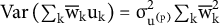 $\mathrm{Var}\left({\sum}_{\mathrm{k}}{\overline{\mathrm{w}}}_{\mathrm{k}}{\mathrm{u}}_{\mathrm{k}}\right)={\unicode{x3c3}}_{{\mathrm{u}}^{\left(\mathrm{p}\right)}}^2{\sum}_{\mathrm{k}}{\overline{\mathrm{w}}}_{\mathrm{k}}^2$
, where
$\mathrm{Var}\left({\sum}_{\mathrm{k}}{\overline{\mathrm{w}}}_{\mathrm{k}}{\mathrm{u}}_{\mathrm{k}}\right)={\unicode{x3c3}}_{{\mathrm{u}}^{\left(\mathrm{p}\right)}}^2{\sum}_{\mathrm{k}}{\overline{\mathrm{w}}}_{\mathrm{k}}^2$
, where
 ${\overline{\mathrm{w}}}_{\mathrm{k}}$
denotes the average weight of party k across governments.
${\overline{\mathrm{w}}}_{\mathrm{k}}$
denotes the average weight of party k across governments.
4.4.2 The Effect of Parties’ Economic Dependence
Table 2 reports the results from three models that examine the effect of parties’ economic dependence on government survival. Model 1 is an SLM in which the party-level variable is aggregated to the government level prior to estimation using the arithmetic mean. Model 2 is an MMMM that accounts for dependencies among governments due to shared parties but also aggregates the party-level variable using the arithmetic mean. Model 3 extends the MMMM by introducing endogenous party weights to dynamically aggregate the party-level variable.
Results from three accelerated failure time Weibull survival models.

Models are estimated using Bayesian MCMC. Details on convergence and model fit are provided in Section A4 of the Supplementary Material. Reported are the posterior medians with their median absolute deviations in parentheses. The party-level variance is calculated as
 $\mathrm{Var}\left({\sum}_{\mathrm{k}}{\overline{\mathrm{w}}}_{\mathrm{k}}{\mathrm{u}}_{\mathrm{k}}\right)={\unicode{x3c3}}_{{\mathrm{u}}^{\left(\mathrm{p}\right)}}^2{\sum}_{\mathrm{k}}{\overline{\mathrm{w}}}_{\mathrm{k}}^2$
, where
$\mathrm{Var}\left({\sum}_{\mathrm{k}}{\overline{\mathrm{w}}}_{\mathrm{k}}{\mathrm{u}}_{\mathrm{k}}\right)={\unicode{x3c3}}_{{\mathrm{u}}^{\left(\mathrm{p}\right)}}^2{\sum}_{\mathrm{k}}{\overline{\mathrm{w}}}_{\mathrm{k}}^2$
, where
 ${\overline{\mathrm{w}}}_{\mathrm{k}}$
denotes the average weight of party k across governments.
${\overline{\mathrm{w}}}_{\mathrm{k}}$
denotes the average weight of party k across governments.
In line with theoretical expectations, coalition governments whose parties are more economically dependent on their members have shorter lifespans. The SLM (M1) estimates this effect at −0.25, with a mean absolute deviation (MAD) of 0.07 and 95% credible interval (CI) of [−0.39, −0.11]. This places the magnitude of the effect on par with that of majority status. By contrast, the MMMM (M2) estimates the effect at −0.37, with a MAD of 0.13 and a CI of [−0.62, −0.13], nearly 1.5 times larger. The differences between M1 and M2 illustrate that, in empirical settings with a limited number of observations, ignoring the multiple-membership structure can bias both point and uncertainty estimates, potentially leading to misleading conclusions.
The MMMM with endogenous party weights (M3) estimates the effect at −0.37, with a MAD of 0.13 and CI of [−0.60, −0.12]. Both the point estimate and the uncertainty remain unchanged, indicating that modeling the aggregation does not come at the cost of increased uncertainty. The estimated effect is substantial: on average, a 10-percentage-point increase in member funding shortens coalition duration by about 154 days (linear approximation; average marginal effect). M3 also fits the data better than M2, with a deviance information criterion (DIC) that is 9 points lower.
In conclusion, while modeling the multiple-membership structure comes at the cost of increased model complexity (
 ${\mathrm{DIC}}_{\mathrm{M}2}=3869>{\mathrm{DIC}}_{\mathrm{M}1}=3844$
), it is essential for obtaining accurate estimates. The comparison between M2 and M3 demonstrates that modeling the aggregation process does not reduce estimate precision (
${\mathrm{DIC}}_{\mathrm{M}2}=3869>{\mathrm{DIC}}_{\mathrm{M}1}=3844$
), it is essential for obtaining accurate estimates. The comparison between M2 and M3 demonstrates that modeling the aggregation process does not reduce estimate precision (
 ${\mathrm{M}\mathrm{AD}}_{\mathrm{M}3,{\unicode{x3b2}}^{\left(\mathrm{ed}\right)}}={\mathrm{M}\mathrm{AD}}_{\mathrm{M}2,{\unicode{x3b2}}^{\left(\mathrm{ed}\right)}}=0.13$
) and improves overall model fit (
${\mathrm{M}\mathrm{AD}}_{\mathrm{M}3,{\unicode{x3b2}}^{\left(\mathrm{ed}\right)}}={\mathrm{M}\mathrm{AD}}_{\mathrm{M}2,{\unicode{x3b2}}^{\left(\mathrm{ed}\right)}}=0.13$
) and improves overall model fit (
 ${\mathrm{DIC}}_{\mathrm{M}3}=3869<{\mathrm{DIC}}_{\mathrm{M}2}=3878$
). Moreover, as I will show next, modeling the aggregation process offers not only statistical benefits but also valuable theoretical insights.
${\mathrm{DIC}}_{\mathrm{M}3}=3869<{\mathrm{DIC}}_{\mathrm{M}2}=3878$
). Moreover, as I will show next, modeling the aggregation process offers not only statistical benefits but also valuable theoretical insights.
4.4.3 The Interdependence Structure of Government Survival
M3 models party weights as a function of parties’ internal ideological cohesion, rather than relying on fixed mean aggregation. The estimated effect of intraparty cohesion is −0.93, with a MAD of 0.47 and CI of [−1.92, −0.12], indicating that more cohesive parties receive lower weights in the aggregated party effect. Panel A of Figure 7 illustrates this relationship. For example, in a three-party coalition where one party is one standard deviation less cohesive than average and the other two have average cohesion, M3 estimates the weights as
 $\mathrm{w}\approx \left(\mathrm{0.46,0.27,0.27}\right)$
. In this scenario, the less cohesive party carries greater weight in determining how economic dependence affects government survival. By contrast, mean aggregation assigns equal weights
$\mathrm{w}\approx \left(\mathrm{0.46,0.27,0.27}\right)$
. In this scenario, the less cohesive party carries greater weight in determining how economic dependence affects government survival. By contrast, mean aggregation assigns equal weights
 $\mathrm{w}=\left(0.\overline{3},0.\overline{3},0.\overline{3}\right)$
, thereby overstating the importance of more cohesive parties and understating that of the less cohesive one. Panel B of Figure 7 illustrates the bias introduced by mean aggregation.
$\mathrm{w}=\left(0.\overline{3},0.\overline{3},0.\overline{3}\right)$
, thereby overstating the importance of more cohesive parties and understating that of the less cohesive one. Panel B of Figure 7 illustrates the bias introduced by mean aggregation.
Predicted party weights by intraparty cohesion. Panel A displays the predicted weights across governments, with the blue line indicating the average weight at each level of cohesion. Panel B depicts the bias introduced by mean aggregation.

In conclusion, this application illustrates that party weights are not always uniform, challenging the arithmetic mean as the default aggregation function.
5 Conclusion
Research on coalition governments has increasingly focused on party-level explanations of coalition outcomes (Giannetti and Benoit Reference Giannetti, Benoit, Giannetti and Benoit2009). This research, however, does not account for the complex multilevel structure between parties and governments. In this article, I show that the crisscrossing relationship between parties and governments implies dependencies among observations that require statistical control and warrant theoretical examination. I then advance a multilevel model that allows researchers to tackle both issues and demonstrate its utility with a simulation study and an empirical application. The simulation study reveals substantial biases, primarily in uncertainty estimates, across all levels of analysis when ignoring party-level dependencies in coalition research. These biases affect both false positive and negative error rates and can thus lead to erroneous conclusions. In contrast, the extended MMMM not only recovers accurate parameter estimates in the presence of party-level clustering but also enables researchers to examine the interplay between coalition parties in their effect on government outcomes. The empirical application shows that coalition governments with parties more dependent on their members have shorter lifespans, and that this effect is shaped disproportionally by parties with low internal cohesion.
The proposed modeling approach has limitations. It requires sufficient data to model complex aggregation processes, proper specification of the weight function to avoid model nonidentification or degeneracy, and a correctly specified multilevel structure to prevent bias in the random effect estimator.
Acknowledgments
I am indebted to Jeroen Weesie, an early collaborator on this project. I also thank Alec McGail, Alison Schultz, Daniel Gotthardt, David Kretschmer, Filiz Garip, George Leckie, Jeff Gill, Lanny Martin, Markus Wagner, Mirjam Moerbeek, Thomas Meyer, Thomas Saalfeld, Tyler Simko, Zac Greene, as well as Daniel Hopkins and three anonymous reviewers for their incredibly valuable feedback. An early version of this article was presented at the 2019 APSA Annual Meeting.
Funding
The author received no specific funding for this research.
Data Availability Statement
Replication code for this article has been published in the Political Analysis Harvard Dataverse at https://doi.org/10.7910/DVN/OB2GXR (Rosche Reference Rosche2026).
Competing Interests
The author declares none.
Supplementary material
To view supplementary material for this article, please visit http://doi.org/10.1017/pan.2026.10039.
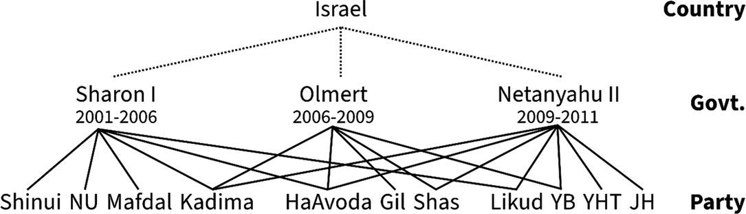
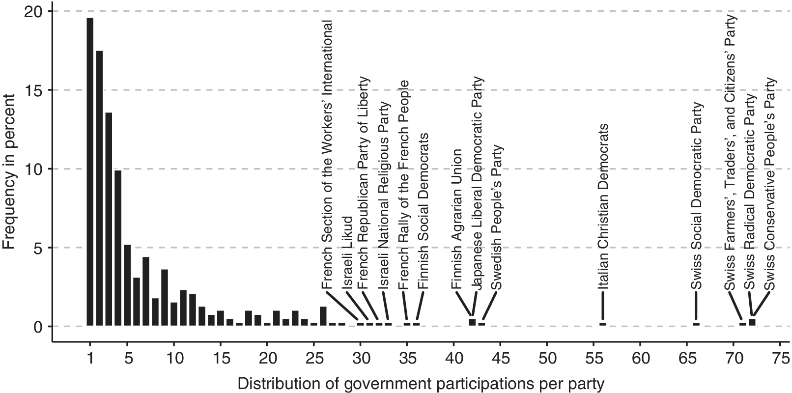
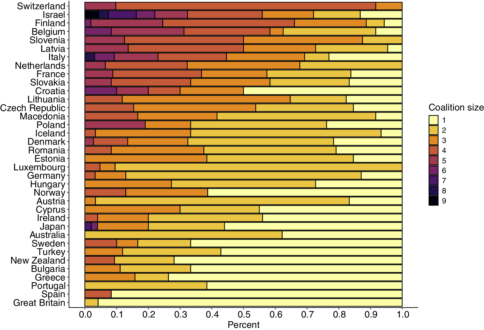
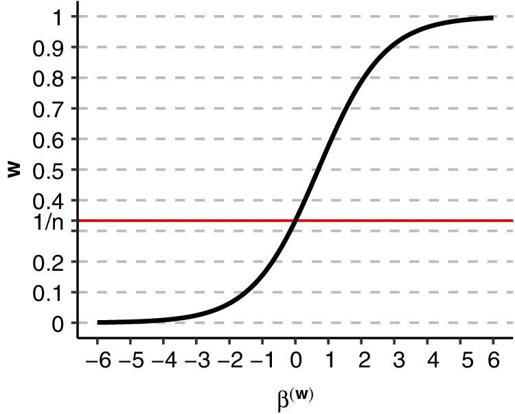


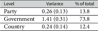
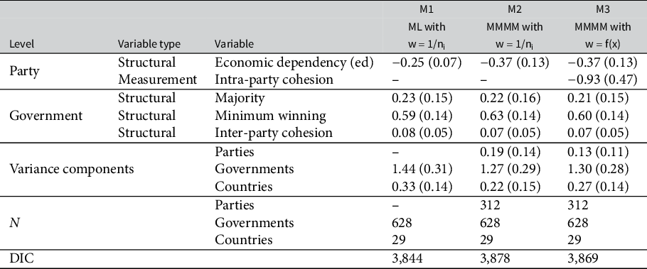


 Open access