


1. Introduction
This section gives an introduction to the study by providing a summary of modelling strategies and fairness measures. Furthermore, this section details the purpose of this study, which is primarily to design a benchmarking framework for assessing pricing fairness and accuracy simultaneously.
1.1 Non-Life Insurance Premium Pricing
Insurance is the business of transferring risk for a premium, and as such, it requires suitable methodologies to evaluate an appropriate value for transferring the risk. The standard approach for evaluating this appropriate value remains the generalised linear model (GLM) (De Jong & Heller, Reference De Jong and Heller2008; Frees, Reference Frees2015; Haberman & Renshaw, Reference Haberman and Renshaw1996; Henckaerts et al., Reference Henckaerts, Côté, Antonio and Verbelen2021; Nelder & Wedderburn, Reference Nelder and Wedderburn1972). The GLM combines information collected about the policy, policyholder and vehicle in a linear representation to describe claims frequencies, claims severities or other quantities of interest that characterise the risk associated with a given policyholder. Under appropriate assumptions, the GLM yields statistically unbiased estimates (McCullagh & Nelder, Reference McCullagh and Nelder1989) and allows for straightforward interpretation, a critical requirement for both the underwriter and policyholder.
The most conventional dual GLM approach consists of modelling claims frequencies and severities separately before recombining the respective estimates into a single premium estimate. It is based on two separate models, typically using a discrete distribution for frequency modelling and a continuous distribution for severity modelling (Campo & Antonio, Reference Campo and Antonio2022; Henckaerts et al., Reference Henckaerts, Côté, Antonio and Verbelen2021; Noll et al., Reference Noll, Salzmann and Wuthrich2020; Ohlsson & Johansson, Reference Ohlsson and Johansson2010). The important theoretic property of unbiasedness at the portfolio level (McCullagh & Nelder, Reference McCullagh and Nelder1989; Wüthrich, Reference Wüthrich2020), along with the transparency and ease of interpretation of linear regression models, contributes to the predominance of GLM approach in non-life insurance pricing. This is despite some well-known limitations, such as the underlying assumption of a simplistic (linear) functional structure of the response variable, which may be unrealistic, making it difficult to incorporate complex interactions and non-linear associations (Campo & Antonio, Reference Campo and Antonio2022; Henckaerts & Antonio, Reference Henckaerts and Antonio2022; König & Loser, Reference König and Loser2020; Spedicato et al., Reference Spedicato, Dutang and Petrini2018). Another limitation is the propensity of the GLM model to overfit with an increase in the number of variables used (McCullagh & Nelder, Reference McCullagh and Nelder1989). Given the growing amount of data available, the propensity of the GLM model to overfit should be considered where pricing is based on large tabulated variables, a common practice in the field (Campo & Antonio, Reference Campo and Antonio2022).
An alternative GLM approach based on a Tweedie distribution is also, but less commonly, considered (Campo & Antonio, Reference Campo and Antonio2022; Marin-Galiano & Christmann, Reference Marin-Galiano and Christmann2004) where premiums are modelled directly by compounding frequency and severity information into a single (Tweedie) random variable. This approach can also be used to capture zero-inflated claims distributions, which, unlike in the conventional dual GLM approach, allows the use of the entire dataset to characterise the risk associated with policyholder profiles with no claims in the portfolio. The joint frequency-severity distribution is controlled by a power parameter, which implicitly assumes a level of correlation between the two quantities and imposes a particular shape on that distribution, which can limit the flexibility of the fitting procedure (Kurz, Reference Kurz2017). There is increasing interest in exploring alternative modelling strategies which can better exploit policyholder information so as to leverage non-linear associations between variables.
1.2 Alternative Modelling Strategies
ML modelling strategies can provide competitive alternatives to GLM, and improve risk stratification in non-life insurance pricing (Campo & Antonio, Reference Campo and Antonio2022; Dal Pozzolo et al., Reference Dal Pozzolo, Moro, Bontempi and Le Borgne2011; Guelman, Reference Guelman2012; Henckaerts et al., Reference Henckaerts, Côté, Antonio and Verbelen2021;Wuthrich & Buser, Reference Wuthrich and Buser2023). Early ML models for pricing included tree-based approaches, as they alleviate the requirement of stringent model assumptions, albeit to the detriment of model interpretability. Regression tree and boosted tree models were considered for claims frequency prediction (Henckaerts et al., Reference Henckaerts, Côté, Antonio and Verbelen2021; Noll et al., Reference Noll, Salzmann and Wuthrich2020). Noll et al. (Reference Noll, Salzmann and Wuthrich2020) demonstrated that feature interactions were captured more effectively using tree-based techniques than with GLM. Henckaerts et al. (Reference Henckaerts, Côté, Antonio and Verbelen2021) compared GLM against various decision trees, random forests (RFs) and boosted trees for pricing, showcasing visualisation tools to obtain insights from the resulting models and their economic value. The loss of model interpretability of ML techniques is usually somewhat mitigated by some form of sensitivity analysis based, for example, on variable importance or partial dependency plots (Henckaerts et al., Reference Henckaerts, Côté, Antonio and Verbelen2021; Kuo & Lupton, Reference Kuo and Lupton2020). Alternative ML approaches include technical adaptations of GLM, for instance, adding a LASSO or elastic net regularisation penalty to mitigate overfitting (Devriendt et al., Reference Devriendt, Antonio, Reynkens and Verbelen2021). Such regularisation procedures, however, still imply using a specific parametric distribution model.
Some studies have explored the potential of neural networks (NN) for pricing. Such studies include the study of use of a shallow feed-forward NN (Noll et al., Reference Noll, Salzmann and Wuthrich2020), an exploration of the value of autoencoders for pricing and premium bias correction (Blier-Wong et al., Reference Blier-Wong, Cossette, Lamontagne and Marceau2022; Grari et al., Reference Grari, Charpentier and Detyniecki2022; Wüthrich & Merz, Reference Wüthrich and Merz2022) and a framework based on generative adversarial networks to synthesise insurance datasets (Kuo, Reference Kuo2019). NN models can approximate non-linear functions very effectively but may appear overly elaborate to analyse portfolios with a small number of variables (Noll et al., Reference Noll, Salzmann and Wuthrich2020; Wüthrich, Reference Wüthrich2020). Wüthrich (Reference Wüthrich2020) argued that NNs may provide pricing accuracy at the individual policy level but that state-of-the-art use of NNs does not assess unbiasedness (pricing fairness) at the portfolio level, which may be controlled with an early stopping rule in the gradient descent.
1.3 Pricing Fairness
Pricing fairness has always been a concern for insurance companies and is mainly understood in terms of premium bias and the nature of the policyholder information used (European Insurance and Occupational Pensions Authority, 2023b; Financial Conduct Authority, 2021). Attention towards pricing fairness is growing further with the development of ML-based pricing models that aim to improve risk differentiation for pricing (Henckaerts et al., Reference Henckaerts, Côté, Antonio and Verbelen2021; Kuo & Lupton, Reference Kuo and Lupton2020) without paying appropriate attention towards pricing fairness. ML models may not systematically result in fairer premiums because of less interpretability as compared to GLM. With the advent of ML models, more efforts are needed to control unlawful discrimination against specific customer groups (Baumann & Loi, Reference Baumann and Loi2023; Lindholm et al., Reference Lindholm, Richman, Tsanakas and Wuthrich2022b). The European Insurance and Occupational Pensions Authority (EIOPA) focused in particular on the use of protected characteristics such as tenure and gender, advocating for increasing sophistication of risk management and governance processes (European Insurance and Occupational Pensions Authority, 2023a). For the purpose of pricing fairness, the Central Bank of Ireland (CBI)’s consumer protection framework was revised to mitigate the risks emerging from the use of innovative models (Central Bank of Ireland, 2024).
Some examples of generic guidelines for the promotion of fairness in pricing include: using a statistical model that is free of proxy discrimination, such that the dependent variable $Y$
(claims frequency, severity or policy premium) is sufficiently well described by non-protected information
$Y$
(claims frequency, severity or policy premium) is sufficiently well described by non-protected information $X$
on the policyholder and product alone (Lindholm et al., Reference Lindholm, Richman, Tsanakas and Wuthrich2022b); the use of an empirical microeconomic framework to evaluate the impact of fairness and accountability in the entire insurance pricing process (Shimao & Huang, Reference Shimao and Huang2022); the use of sets of fairness criteria (e.g. fairness through unawareness and through awareness, counterfactual fairness, independence from protected characteristics, etc.) to evaluate discriminatory effects on specific features or groups of policyholder profiles (Lindholm et al., Reference Lindholm, Richman, Tsanakas and Wuthrich2022a; Mosley & Wenman, Reference Mosley and Wenman2022; Xin & Huang, Reference Xin and Huang2024); and the use of methods to remove various types of biases, through either pre-, in- or post-processing (Becker et al., Reference Becker, Jentzen, Müller and von Wurstemberger2022; Denuit et al., Reference Denuit, Charpentier and Trufin2021; Mosley & Wenman, Reference Mosley and Wenman2022; Wüthrich, Reference Wüthrich2020).
$X$
on the policyholder and product alone (Lindholm et al., Reference Lindholm, Richman, Tsanakas and Wuthrich2022b); the use of an empirical microeconomic framework to evaluate the impact of fairness and accountability in the entire insurance pricing process (Shimao & Huang, Reference Shimao and Huang2022); the use of sets of fairness criteria (e.g. fairness through unawareness and through awareness, counterfactual fairness, independence from protected characteristics, etc.) to evaluate discriminatory effects on specific features or groups of policyholder profiles (Lindholm et al., Reference Lindholm, Richman, Tsanakas and Wuthrich2022a; Mosley & Wenman, Reference Mosley and Wenman2022; Xin & Huang, Reference Xin and Huang2024); and the use of methods to remove various types of biases, through either pre-, in- or post-processing (Becker et al., Reference Becker, Jentzen, Müller and von Wurstemberger2022; Denuit et al., Reference Denuit, Charpentier and Trufin2021; Mosley & Wenman, Reference Mosley and Wenman2022; Wüthrich, Reference Wüthrich2020).
There are multiple measures of fairness, but not all measures of fairness and accuracy can be satisfied simultaneously (Baumann & Loi, Reference Baumann and Loi2023; Frees & Huang, Reference Frees and Huang2023; Iturria, Reference Iturria2023; Lindholm et al., Reference Lindholm, Richman, Tsanakas and Wüthrich2024b). In practice, fairness issues are often framed in terms of market behaviour, such as targeting specific customer groups (such as young drivers) or through “price walking.” The Central Bank of Ireland (2022) “price walking” defines “price walking” as a practice where a customer’s premium is gradually increased in longer-term policies. Formally, one could think of a fair premium as one that is as close to the true underlying risk of that individual as possible, adopting a risk-based pricing (Xin & Huang, Reference Xin and Huang2024). The literature on individual fairness is scarce, and is primarily focused on group fairness, with a range of complementary definitions that predominantly include demographic parity (whereby premium distributions should be equal across protected groups overall), actuarial group fairness (whereby premium distributions should be equal across protected groups for any given risk profile) and calibration (in the sense that for a given predicted risk level, the actual risk should be the same across protected groups) (Barocas et al., Reference Barocas, Hardt and Narayanan2023; Dolman & Semenovich, Reference Dolman and Semenovich2018; Dwork et al., Reference Dwork, Hardt, Pitassi, Reingold and Zemel2011; Kleinberg et al., Reference Kleinberg, Mullainathan and Raghavan2016; Lindholm et al., Reference Lindholm, Lindskog and Palmquist2023; Xin & Huang, Reference Xin and Huang2024). Attaining demographic parity does not eliminate unfairness at the individual level, as individuals from lower-risk groups may end up paying more than they should, while those from higher-risk groups might pay less than their risk would warrant (Dwork et al., Reference Dwork, Hardt, Pitassi, Reingold and Zemel2011). Similarly, achieving actuarial group fairness ensures similar outcomes across protected groups within bands of homogeneous risk, but may sometimes make the overall model less accurate (Dolman & Semenovich, Reference Dolman and Semenovich2018). Another fairness metric called “disparate impact” consists of evaluating whether outcomes affect one group more than others (Barocas et al., Reference Barocas, Hardt and Narayanan2023). Optimising for “disparate impact” may reduce accuracy by forcing similar outcomes across groups with different risk profiles (Xin & Huang, Reference Xin and Huang2024).
Improving model fairness may thus impact other aspects of model performance depending on the model and the criteria being considered. Although model performance has been considered in GLM and a number of other modelling strategies (Colella & Jones, Reference Colella and Jones2023; Fauzan & Murfi, Reference Fauzan and Murfi2018; Ferrario & Hämmerli, Reference Ferrario and Hämmerli2019; Henckaerts et al., Reference Henckaerts, Côté, Antonio and Verbelen2021; Kuo & Lupton, Reference Kuo and Lupton2020), towards, an overall picture of model performance combining predictive potential and fairness is rarely evaluated using a comparative benchmark. At the time of writing, we are only aware of one other paper reporting on such a combined assessment of fairness and pricing accuracy (Xin & Huang, Reference Xin and Huang2024). Furthermore, the majority of published research concentrates on classification settings, evaluating fairness in binary decisions (see Dolman & Semenovich, Reference Dolman and Semenovich2018; Lindholm et al., Reference Lindholm, Richman, Tsanakas and Wuthrich2022a and references within). Fairness in insurance pricing, treated as a regression problem, remains scarcely explored. This paper aims to narrow this gap in the literature. The subsection below details the goal and contribution of this paper.
1.4 Goals and Contribution
The aim of this work is to assess the potential benefits of ML-based pricing solutions against the current industry standard GLM-based approach in a regression setting. Recent papers report on studies of fairness that capture some aspects of the analyses proposed in this paper (for example, these studies may consider performance of the product model, or focus on fairness criteria) (Lindholm et al., Reference Lindholm, Richman, Tsanakas and Wuthrich2022a, Reference Lindholm, Richman, Tsanakas and Wüthrich2024b; Moriah et al., Reference Moriah, Vermet and Charpentier2024). The proposed study brings together multiple aspects into a comprehensive comparative analysis of popular ML models, evaluating both model performance and pricing fairness simultaneously. This framework is described in Section 2. The performance benchmark used for this study is not unlike that of Henckaerts et al. (Reference Henckaerts, Côté, Antonio and Verbelen2021) However, Henckaerts et al. (Reference Henckaerts, Côté, Antonio and Verbelen2021) in their work used only a Poisson-gamma modelling strategy, whereas we extend the evaluation to include a Tweedie modelling strategy. Our assessment of pricing fairness combines the approach carried out by the Central Bank of Ireland (Central Bank of Ireland, 2022) with three common fairness metrics for demographic parity, group fairness and calibration (Dolman & Semenovich, Reference Dolman and Semenovich2018). We define these metrics with respect to conditional distributions of raw actual premiums in Section 2.5.9, and propose a practical quantitation for these three axioms. The models are compared on two open-source datasets in Section 3 to evaluate methods on two distinct common types of cover: third-party liability and fully comprehensive liability. Section 4 presents the details of a fairness analysis carried out on the second dataset. The findings of this study are discussed further in Section 5 and demonstrate that ML strategies provide consistent improvements over GLM, but also that there is not necessarily one optimal ML model for non-life premium pricing. Furthermore, Section 5 also illustrates that ML strategies can yield better performance, which can be achieved together with improvement in various fairness criteria.
2. Premium Modelling and Assessment
This section describes the premium modelling methodology and defines the key performance indicators and measures of pricing fairness considered for this study.
2.1 Quantities of Interest
We consider a portfolio of $n$
independent policies with data
$n$
independent policies with data ${{\bf({D}}_i},{{\bf{Z}}_i},{N_i},{L_i},{e_i})$
,
${{\bf({D}}_i},{{\bf{Z}}_i},{N_i},{L_i},{e_i})$
, $\forall $ $i = 1, \ldots, n$
, where:
$i = 1, \ldots, n$
, where:
- ${\bf{D}}$
denotes a vector of unprotected policyholder information (e.g. vehicle age, area, etc.), which can be used to rate on,
${\bf{D}}$
denotes a vector of unprotected policyholder information (e.g. vehicle age, area, etc.), which can be used to rate on, -
${\bf{Z}}$
denotes protected policyholder variables (e.g. gender, ethnicity, etc.), which may not be used for pricing,
-
$N$
and
$L,$
respectively, denote the number of claims and the aggregated claims amount for each policy over its exposure
$e$
.


In what follows, we will in turn use either the unprotected policyholder data matrix ${\bf{X}} = {\bf{D}}$
, or the combined
${\bf{X}} = {\bf{D}}$
, or the combined $n \times p$
data matrix
$n \times p$
data matrix ${\bf{X}} = \left[ {{\bf{D}},{\bf{Z}}} \right]$
comprising of both
${\bf{X}} = \left[ {{\bf{D}},{\bf{Z}}} \right]$
comprising of both ${\bf{D}}$
and
${\bf{D}}$
and ${\bf{Z}}$
. The nature of protected variables varies by jurisdiction and laws applicable in the country. In this paper, we consider fairness with respect to gender, a typical variable that is protected in Ireland. Factors such as gender, age and marital status are considered protected characteristics under EU anti-discrimination law. However, gender has a unique status among these protected characteristics; regardless of its commercial or underwriting relevance to insurance risks, it cannot be used in setting insurance prices (European Parliamentary Research Service, 2017).
${\bf{Z}}$
. The nature of protected variables varies by jurisdiction and laws applicable in the country. In this paper, we consider fairness with respect to gender, a typical variable that is protected in Ireland. Factors such as gender, age and marital status are considered protected characteristics under EU anti-discrimination law. However, gender has a unique status among these protected characteristics; regardless of its commercial or underwriting relevance to insurance risks, it cannot be used in setting insurance prices (European Parliamentary Research Service, 2017).
Using this information, we are interested in evaluating the intrinsic policyholder risk
 $${P_T} = \mathbb{E}(L|{\bf{D}},{\bf{Z}})$$
and a best feasible estimate of the expected loss for a policy
 $${P_A} = \mathbb{E}(L|{\bf{D}})$$
Quantities ${P_T}$
and
${P_T}$
and ${P_A}$
can be seen, respectively, as the “best estimate price” and “unaware price” (Lindholm et al., Reference Lindholm, Richman, Tsanakas and Wuthrich2022a), to which the company would apply a number of commercial margins and adjustments to account for expenses, levies, etc. Although
${P_A}$
can be seen, respectively, as the “best estimate price” and “unaware price” (Lindholm et al., Reference Lindholm, Richman, Tsanakas and Wuthrich2022a), to which the company would apply a number of commercial margins and adjustments to account for expenses, levies, etc. Although ${P_T}$
and
${P_T}$
and ${P_A}$
as defined above do not include any such additional margins and adjustments, they provide a basis for intrinsic evaluation of risk/loss. For the sake of simplicity, and as described in other works (Lindholm et al., Reference Lindholm, Richman, Tsanakas and Wüthrich2024b) in the rest of the paper, we refer to
${P_A}$
as defined above do not include any such additional margins and adjustments, they provide a basis for intrinsic evaluation of risk/loss. For the sake of simplicity, and as described in other works (Lindholm et al., Reference Lindholm, Richman, Tsanakas and Wüthrich2024b) in the rest of the paper, we refer to ${P_T}$
and
${P_T}$
and ${P_A},$
respectively, as technical premium (TP) and actual premium (AP). In this work, we consider two distinct modelling strategies to estimate
${P_A},$
respectively, as technical premium (TP) and actual premium (AP). In this work, we consider two distinct modelling strategies to estimate ${P_T}$
and
${P_T}$
and ${P_A}$
, namely, the Poisson-gamma (product) model, and the Tweedie model.
${P_A}$
, namely, the Poisson-gamma (product) model, and the Tweedie model.
2.2 Poisson-gamma (Product) Model
The first modelling strategy considered is the most prevalent, Poisson-gamma (product) model. This strategy consists of estimating frequency and severity as two separate steps. Claims frequencies are typically modelled by a discrete count distribution. The Poisson distribution being a common choice (Henckaerts et al., Reference Henckaerts, Côté, Antonio and Verbelen2021; Noll et al., Reference Noll, Salzmann and Wuthrich2020) and the distribution used hereafter, such that for policyholder $i \in \left\{ {1, \ldots, n} \right\}$
,
$i \in \left\{ {1, \ldots, n} \right\}$
,
 $${N_i}\sim Poi\left( {{\mu _i}{e_i}} \right),{\rm{\;\;\;\;}}{\mu _i} \gt 0,\;\;{e_i} \gt 0$$
for some rate ${\mu _i}$
. Then the claims frequency
${\mu _i}$
. Then the claims frequency $F$
over a unit period of exposure (say, one-year exposure), i.e. the number of claims
$F$
over a unit period of exposure (say, one-year exposure), i.e. the number of claims $N$
proportional to exposure
$N$
proportional to exposure $e$
, is such that
$e$
, is such that
 $$\mathbb{E}\left( F \right) = \mathbb{E}\left( {{N \over e}\,\left|\, e \right \gt 0} \right)$$
or, for a given policy, evaluated as
 $${F_i} = {{{N_i}} \over {{e_i}}}$$
such that $\mathbb{E}\left( {{F_i}} \right) = {\mu _i}$
and
$\mathbb{E}\left( {{F_i}} \right) = {\mu _i}$
and $Var\left( {{F_i}} \right) = {{{\mu _i}} \over {{e_i}}}$
, i.e.
$Var\left( {{F_i}} \right) = {{{\mu _i}} \over {{e_i}}}$
, i.e. ${F_i}$
is pseudo-Poisson random variable (either over or under-dispersed depending on the sign of
${F_i}$
is pseudo-Poisson random variable (either over or under-dispersed depending on the sign of ${e_i} - 1$
; usually
${e_i} - 1$
; usually ${e_i} \le 1$
). In practice, we can estimate
${e_i} \le 1$
). In practice, we can estimate ${\mu _i}$
as the maximum likelihood estimator (MLE)
${\mu _i}$
as the maximum likelihood estimator (MLE)
 $${\hat \mu _i} = {F_i}$$
A conventional approach consists of fitting a GLM to the policyholder information $\left( {{\bf{D}},{\bf{Z}},N,e} \right)$
to explain claims frequencies for individual profiles as
$\left( {{\bf{D}},{\bf{Z}},N,e} \right)$
to explain claims frequencies for individual profiles as
 $${\rm{log}}\mathbb{E}(F|{\bf{X}}) = {g_F}\left( {\bf{X}} \right) = {\bf{X}}{\beta _F}$$
with real-valued regression coefficients ${\beta _F} \in {\mathbb{R}^p}$
. Model (1) may be fit to the data by minimising the Poisson deviance between claims frequency data
${\beta _F} \in {\mathbb{R}^p}$
. Model (1) may be fit to the data by minimising the Poisson deviance between claims frequency data $\{ {y_i}\} _{i = 1}^n$
(e.g. where
$\{ {y_i}\} _{i = 1}^n$
(e.g. where $Y = F$
) and a set of model predictions
$Y = F$
) and a set of model predictions $\{ {g_F}\left( {{{\bf{x}}_i}} \right)\} _{i = 1}^n$
obtained from policyholder data
$\{ {g_F}\left( {{{\bf{x}}_i}} \right)\} _{i = 1}^n$
obtained from policyholder data ${\bf{X}}$
, defined as in (Henckaerts et al., Reference Henckaerts, Côté, Antonio and Verbelen2021; Venables & Ripley, Reference Venables and Ripley2013) by
${\bf{X}}$
, defined as in (Henckaerts et al., Reference Henckaerts, Côté, Antonio and Verbelen2021; Venables & Ripley, Reference Venables and Ripley2013) by
 $${{\cal D}_F}\left( {y,{g_F}\left( {\bf{X}} \right)} \right) = 2\mathop \sum \limits_{i = 1}^n \left( {{y_i}log\left( {{{{y_i}} \over {{g_F}\left( {{{\bf{x}}_i}} \right)}}} \right) - \left( {{y_i} - {g_F}\left( {{{\bf{x}}_i}} \right)} \right)} \right)$$
Let us then define claim severity $S$
as the aggregated loss (or claim amount)
$S$
as the aggregated loss (or claim amount) $L$
divided by the number of claims from a subset of polices that have at least one or more claims reported and paid out, such that
$L$
divided by the number of claims from a subset of polices that have at least one or more claims reported and paid out, such that
 $$\mathbb{E}\left( S \right) = \mathbb{E}\left( {{L \over N}\,\left|\, N \right\gt 0} \right)$$
or, for a given policy $i$
, evaluated as
$i$
, evaluated as
 $${S_i} = {{{L_i}} \over {{N_i}}}$$
Hereafter, following a conventional approach, $S$
is modelled by a gamma distribution to allow for skewness arising naturally in such data. Similar to equations (1) and (2), claim severities may be modelled using a distinct GLM, that we may denote as
$S$
is modelled by a gamma distribution to allow for skewness arising naturally in such data. Similar to equations (1) and (2), claim severities may be modelled using a distinct GLM, that we may denote as ${g_S}\left( X \right) = {\bf{X}}{\beta _S}$
with
${g_S}\left( X \right) = {\bf{X}}{\beta _S}$
with ${\beta _S} \in {\mathbb{R}^p}$
. This model may be achieved by minimising the gamma deviance between the severity observations
${\beta _S} \in {\mathbb{R}^p}$
. This model may be achieved by minimising the gamma deviance between the severity observations $\{ {y_i}\} _{i = 1}^n$
(e.g. where
$\{ {y_i}\} _{i = 1}^n$
(e.g. where $Y = S$
) and a set of model predictions
$Y = S$
) and a set of model predictions $\{ {g_S}\left( {{{\bf{x}}_i}} \right)\} _{i = 1}^n$
defined as in (Henckaerts et al., Reference Henckaerts, Côté, Antonio and Verbelen2021) by
$\{ {g_S}\left( {{{\bf{x}}_i}} \right)\} _{i = 1}^n$
defined as in (Henckaerts et al., Reference Henckaerts, Côté, Antonio and Verbelen2021) by
 $${{{\cal D}_S}\left\{ {y,{g_S}\left( {\bf{X}} \right)} \right\} = 2\mathop \sum \limits_{i = 1}^n {w_i}\left( {{{{y_i} - {g_S}\left( {{{\bf{x}}_i}} \right)} \over {{g_S}\left( {{{\bf{x}}_i}} \right)}} - {\rm{log}}\left( {{{{y_i}} \over {{g_S}\left( {{{\bf{x}}_i}} \right)}}} \right)} \right)}$$
where ${w_i}$
is the weight for each observation. Hereafter we use
${w_i}$
is the weight for each observation. Hereafter we use ${w_i} = {N_i}$
.
${w_i} = {N_i}$
.
The overall policy premium $P$
may then be defined as the expected loss
$P$
may then be defined as the expected loss $L$
per unit of exposure, such that
$L$
per unit of exposure, such that
 $$P = \mathbb{E}\left( {{L \over e}} \right)$$
under the assumptions of a non-zero chance that a claim be made, and that claim frequencies and severities are independent of each other. A policy premium estimate $\hat P$
over a unit exposure may then be obtained as the product of estimates for frequency
$\hat P$
over a unit exposure may then be obtained as the product of estimates for frequency $\hat F$
and severity
$\hat F$
and severity $\hat S$
(Denuit et al., Reference Denuit, Maréchal, Pitrebois and Walhin2007; Frees et al., Reference Frees, Meyers and Cummings2014; Parodi, Reference Parodi2014), i.e.
$\hat S$
(Denuit et al., Reference Denuit, Maréchal, Pitrebois and Walhin2007; Frees et al., Reference Frees, Meyers and Cummings2014; Parodi, Reference Parodi2014), i.e.
 $$\hat P = \hat F \times \hat S$$
such that (Henckaerts et al., Reference Henckaerts, Côté, Antonio and Verbelen2021)
 $$\mathbb{E}\left( {\hat P} \right) = P = \mathbb{E}\left( {F \times S} \right) = \mathbb{E}\left( {{N \over e}} \right) \times \mathbb{E}\left( {{L \over N}\,\left|\, N \right\gt 0} \right).$$
2.3 Tweedie Model
A relatively common alternative to the Poisson-gamma product model consists of modelling the quantity $\mathbb{E}\left( {\hat P} \right)$
directly as a compound variable under the Tweedie distribution (Quijano Xacur & Garrido, Reference Quijano Xacur and Garrido2015; Shi, Reference Shi2016). This member of the exponential dispersion family is characterised by a variance function of the form
$\mathbb{E}\left( {\hat P} \right)$
directly as a compound variable under the Tweedie distribution (Quijano Xacur & Garrido, Reference Quijano Xacur and Garrido2015; Shi, Reference Shi2016). This member of the exponential dispersion family is characterised by a variance function of the form ${\rm{Var}}\left( Y \right) = \phi {\gamma ^\alpha }$
, where
${\rm{Var}}\left( Y \right) = \phi {\gamma ^\alpha }$
, where $\phi $
is the dispersion parameter,
$\phi $
is the dispersion parameter, $\gamma $
is the mean, and
$\gamma $
is the mean, and $\alpha $
is the power parameter such that
$\alpha $
is the power parameter such that $\alpha \ne 0$
and
$\alpha \ne 0$
and $\alpha \ne 1$
. Given a set of
$\alpha \ne 1$
. Given a set of $n$
independent observations
$n$
independent observations $\left\{ {{y_1}, \ldots, {y_n}} \right\}$
of a Tweedie random variable
$\left\{ {{y_1}, \ldots, {y_n}} \right\}$
of a Tweedie random variable $Y,$
an estimate of the premium
$Y,$
an estimate of the premium $P$
is derived by minimising the Tweedie deviance between the observations
$P$
is derived by minimising the Tweedie deviance between the observations $\{ {y_i}\} _{i = 1}^n$
and a set of model predictions
$\{ {y_i}\} _{i = 1}^n$
and a set of model predictions $\{ {g_T}\left( {{{\bf{x}}_i}} \right)\} _{i = 1}^n$
, defined as
$\{ {g_T}\left( {{{\bf{x}}_i}} \right)\} _{i = 1}^n$
, defined as
 $${{\cal D}\left( {y,{g_T}\left( {\bf{X}} \right)} \right) = \mathop \sum \limits_{i = 1}^n {2 \over \phi }\left( {{{y_i^{2 - \alpha }} \over {\left( {1 - \alpha } \right)\left( {2 - \alpha } \right)}} - {{{y_i}{g_T}{{({{\bf{x}}_i})}^{1 - \alpha }}} \over {1 - \alpha }} + {{{g_T}{{({{\bf{x}}_i})}^{2 - \alpha }}} \over {2 - \alpha }}} \right)}$$
with respect to $\left( {\phi, \gamma, \alpha } \right)$
and the model parameters for
$\left( {\phi, \gamma, \alpha } \right)$
and the model parameters for ${g_T}$
.
${g_T}$
.
2.4 Premium Modelling
A number of models $g\left( {\bf{X}} \right)$
using the Poisson, gamma or Tweedie deviance
$g\left( {\bf{X}} \right)$
using the Poisson, gamma or Tweedie deviance ${\cal D}$
defined, respectively, by equations (2), (3) or (4), as cost function were compared. They include the conventional GLM, with a structure similar to equation (1), allowing for interaction terms (McCullagh & Nelder, Reference McCullagh and Nelder1989; Ohlsson & Johansson, Reference Ohlsson and Johansson2010) in a forward stepwise selection of the final model ESL; an elastic net and a LASSO (Tibshirani, Reference Tibshirani1996; Zou & Hastie, Reference Zou and Hastie2005), using
${\cal D}$
defined, respectively, by equations (2), (3) or (4), as cost function were compared. They include the conventional GLM, with a structure similar to equation (1), allowing for interaction terms (McCullagh & Nelder, Reference McCullagh and Nelder1989; Ohlsson & Johansson, Reference Ohlsson and Johansson2010) in a forward stepwise selection of the final model ESL; an elastic net and a LASSO (Tibshirani, Reference Tibshirani1996; Zou & Hastie, Reference Zou and Hastie2005), using $\delta = 0.5$
and
$\delta = 0.5$
and $\delta = 1$
, respectively, and a regularisation parameter
$\delta = 1$
, respectively, and a regularisation parameter $\lambda \gt 0$
in
$\lambda \gt 0$
in
 $${{\cal D}_\lambda }\left( {\hat \beta } \right) = \mathop \sum \limits_{i = 1}^n \,{\cal D}{({y_i},{{\bf{x}}_i}{{\hat \beta} _j})^2} + \lambda \mathop \sum \limits_{j = 1}^p \,\left( {{1 \over 2}\left( {1 - \delta } \right)\beta _j^2 + \delta \left| {{\beta _{\rm{j}}}} \right|} \right)$$
Furthermore, they also include a pruned regression tree (Breiman et al., Reference Breiman, Friedman, Stone and Olshen1984; Friedman, Reference Friedman2001) partitioning the dataset into $J$
leafs
$J$
leafs $R = \left\{ {{R_1}, \ldots, {R_J}} \right\}$
and with complexity penalisation
$R = \left\{ {{R_1}, \ldots, {R_J}} \right\}$
and with complexity penalisation $c \gt 0$
as described in (Henckaerts et al., Reference Henckaerts, Côté, Antonio and Verbelen2021) by optimising
$c \gt 0$
as described in (Henckaerts et al., Reference Henckaerts, Côté, Antonio and Verbelen2021) by optimising

where ${\hat y_R}$
denotes the average value of
${\hat y_R}$
denotes the average value of $Y$
within a leaf or set of leaves
$Y$
within a leaf or set of leaves $R$
as defined above; a RF (Breiman, Reference Breiman2001) using an ensemble of
$R$
as defined above; a RF (Breiman, Reference Breiman2001) using an ensemble of $M$
trees; a gradient boosting model (GBM) (Friedman, Reference Friedman2001) using a penalised loss gradient at each step
$M$
trees; a gradient boosting model (GBM) (Friedman, Reference Friedman2001) using a penalised loss gradient at each step $m = 2, \ldots, M$
, the latter being defined by
$m = 2, \ldots, M$
, the latter being defined by
 $$ - {g_m}\left( {\bf{x}} \right) = - {\left[ {{{\partial {\cal D}\left( {y,g\left( {\bf{x}} \right)} \right)} \over {\partial g\left( {\bf{x}} \right)}}} \right]_{g\left( {\bf{x}} \right) = {g_{m - 1}}\left( {\bf{x}} \right)}}$$
as well as extreme gradient boosting (XGB) (Chen & Guestrin, Reference Chen and Guestrin2016), penalising (a second-order linearisation of) the deviance by
 $$\mathop \sum \limits_{i = 1}^n \,{\cal D}\left( {{y_i},g\left( {{{\bf{x}}_i}} \right)} \right) + \xi J + {\tau \over 2}\left| {\left| \omega \right|} \right|$$
where $J$
is the number of terminal nodes or leaves in a tree,
$J$
is the number of terminal nodes or leaves in a tree, $\xi \gt 0$
a user defined penalty encouraging pruning, and for some regularisation
$\xi \gt 0$
a user defined penalty encouraging pruning, and for some regularisation $\tau \gt 0$
of the final leaf weights
$\tau \gt 0$
of the final leaf weights $\omega $
determined for the ensemble model by stochastic gradient descent. XGB in particular has gained a lot of popularity in the actuarial field in recent years, some research reporting it to outperform other models for insurance claims and frequency prediction (Colella & Jones, Reference Colella and Jones2023; Fauzan & Murfi, Reference Fauzan and Murfi2018; Ferrario & Hämmerli, Reference Ferrario and Hämmerli2019; Henckaerts et al., Reference Henckaerts, Côté, Antonio and Verbelen2021; Kuo & Lupton, Reference Kuo and Lupton2020).
$\omega $
determined for the ensemble model by stochastic gradient descent. XGB in particular has gained a lot of popularity in the actuarial field in recent years, some research reporting it to outperform other models for insurance claims and frequency prediction (Colella & Jones, Reference Colella and Jones2023; Fauzan & Murfi, Reference Fauzan and Murfi2018; Ferrario & Hämmerli, Reference Ferrario and Hämmerli2019; Henckaerts et al., Reference Henckaerts, Côté, Antonio and Verbelen2021; Kuo & Lupton, Reference Kuo and Lupton2020).
2.5 Performance Evaluation
2.5.1 Resampling Framework
Prior to the analyses, each of the two datasets considered in Section 3 were split randomly into a build sample and a test sample, comprising, respectively, 83% and 17% of the complete dataset. This random splitting was done to ensure that each of the cross-validation folds contained roughly the same amount of data as the test set. The build set was used for model training using nested 5-fold cross-validation (CV) (Hastie et al., Reference Hastie, Tibshirani and Friedman2009). The model hyperparameters were set from the CV training folds, via a grid search, to optimise deviance ${\cal D}$
as defined by equations (2), (3) or (4) as appropriate. The performance metrics defined hereafter were then evaluated on each of the five validation folds and averaged to obtain a first measure of performance. The resulting model fits were then applied to the test sample for external model performance evaluation, using .632-bootstrapping ESL to compute standard errors and non-parametric confidence intervals for the performance indicators points from 250 bootstrap resamples.
${\cal D}$
as defined by equations (2), (3) or (4) as appropriate. The performance metrics defined hereafter were then evaluated on each of the five validation folds and averaged to obtain a first measure of performance. The resulting model fits were then applied to the test sample for external model performance evaluation, using .632-bootstrapping ESL to compute standard errors and non-parametric confidence intervals for the performance indicators points from 250 bootstrap resamples.
2.5.2 Post-Modelling Calibration
All model predictions (premium estimates) were calibrated to adjust for model bias before they were used to carry out analysis. The calibration factor $C$
was calculated based on the model fits obtained on the training dataset and is evaluated as
$C$
was calculated based on the model fits obtained on the training dataset and is evaluated as
 $$C = {{\mathop \sum \nolimits_{i = 1}^n \,{L_i}} \over {\mathop \sum \nolimits_{i = 1}^n \,{{\hat P}_i}}}$$
2.5.3 Premium Estimation Error and Bias
All models were first compared on the test set with respect to bootstrapped Poisson, gamma and Tweedie deviances as defined in equations (2), (3) or (4), to evaluate overall model error. Model bias was also evaluated on the test data as the difference between the total sum of observed losses and the premium estimates obtained from each model, defined as
 $$\mathop \sum \limits_{i = 1}^n \,\left( {{L_i} - {{\hat P}_{T,i}}} \right)$$
2.5.4 Risk Stratification
Lorenz curves were used to compare premiums by analysing the distribution of premiums versus losses, where both quantities were ordered by increasing relativities
 $${r_i} = {{{{\hat Q}_i}} \over {{{\hat P}_i}}},{\rm{\;}}i = 1, \ldots, n$$
i.e. by the ratio of the premium prediction obtained from the competing model ( $\hat Q$
) to that of the benchmark model (
$\hat Q$
) to that of the benchmark model ( $\hat P$
) (Henckaerts et al., Reference Henckaerts, Côté, Antonio and Verbelen2021), whose empirical c.d.f. is denoted hereafter by
$\hat P$
) (Henckaerts et al., Reference Henckaerts, Côté, Antonio and Verbelen2021), whose empirical c.d.f. is denoted hereafter by ${F_n}$
. Sorting policies in terms of their increasing relativity, the ordered Lorenz curve then has coordinates
${F_n}$
. Sorting policies in terms of their increasing relativity, the ordered Lorenz curve then has coordinates $\left( {{{\hat F}_L},{{\hat F}_{\hat P}}} \right)$
defined by
$\left( {{{\hat F}_L},{{\hat F}_{\hat P}}} \right)$
defined by
 $${\hat F_{\hat P}}\left( s \right) = {{\mathop \sum \nolimits_{i = 1}^n \,\hat P\left( {{{\bf{x}}_i}} \right)I\left( {{F_n}\left( {{r_i}} \right) \le s} \right)} \over {\mathop \sum \nolimits_{i = 1}^n \,\hat P\left( {{{\bf{x}}_i}} \right)}},{\rm{\;\;}}s \in \left[ {0,1} \right]$$
and
 $${\hat F_L}\left( s \right) = {{\mathop \sum \nolimits_{i = 1}^n \,{y_i}I\left( {{F_n}\left( {{r_i}} \right) \le s} \right)} \over {\mathop \sum \nolimits_{i = 1}^n \,{y_i}}},{\rm{\;\;}}s \in \left[ {0,1} \right]$$
where $I\left( . \right)$
is the indicator function. The curve
$I\left( . \right)$
is the indicator function. The curve $\left( {{{\hat F}_L},{{\hat F}_{\hat P}}} \right)$
follows the identity line
$\left( {{{\hat F}_L},{{\hat F}_{\hat P}}} \right)$
follows the identity line $\left( {y = x} \right)$
in the case of benchmark estimation. The Gini index is calculated as twice the area between the ordered Lorenz curve and the identity line (Frees et al., Reference Frees, Meyers and Cummings2014; Henckaerts et al., Reference Henckaerts, Côté, Antonio and Verbelen2021). Larger index indicates greater risk differentiation can be obtained by using the competing premium
$\left( {y = x} \right)$
in the case of benchmark estimation. The Gini index is calculated as twice the area between the ordered Lorenz curve and the identity line (Frees et al., Reference Frees, Meyers and Cummings2014; Henckaerts et al., Reference Henckaerts, Côté, Antonio and Verbelen2021). Larger index indicates greater risk differentiation can be obtained by using the competing premium $\hat Q$
compared to the reference premium
$\hat Q$
compared to the reference premium $\hat P$
, and hence the competing pricing model is more profitable. This case corresponds to a concave Lorenz curve. The profitability point is as per the theory (Frees et al., Reference Frees, Meyers and Cummings2014) that the profitability is the area under the Lorenz curve. However, if Company B has a better estimate of elasticity and conversion/retention rates then they could operate more profitably than Company A, even if A has the more profitable pricing model. In this analysis, we assume that the price elasticity modelling capabilities between companies are similar and they do not play a role.
$\hat P$
, and hence the competing pricing model is more profitable. This case corresponds to a concave Lorenz curve. The profitability point is as per the theory (Frees et al., Reference Frees, Meyers and Cummings2014) that the profitability is the area under the Lorenz curve. However, if Company B has a better estimate of elasticity and conversion/retention rates then they could operate more profitably than Company A, even if A has the more profitable pricing model. In this analysis, we assume that the price elasticity modelling capabilities between companies are similar and they do not play a role.
2.5.5 Loss Ratios and Conversion Rates in Open-market Competition
A two-player game was implemented to simulate an open-market competition between the industry-standard GLM methodology and each of the competing alternatives for premium prediction. The models are evaluated in terms of their loss ratio (LR) defined as the earned premium ${\hat P_A}$
over paid claims
${\hat P_A}$
over paid claims $L$
(
$L$
( $LR = {{{L_i}} \over {{{\hat P}_{A,i}}}}$
). In this game, for a particular policyholder, the model yielding the lowest premium wins the business and hence secures the premium predicted for the policy as revenue. If
$LR = {{{L_i}} \over {{{\hat P}_{A,i}}}}$
). In this game, for a particular policyholder, the model yielding the lowest premium wins the business and hence secures the premium predicted for the policy as revenue. If $\hat P_{A,i}^{GLM} \lt \hat P_{A,i}^{ML}$
, GLM secures the business, thereby obtaining both the associated revenue and the cost of claims from that policy.
$\hat P_{A,i}^{GLM} \lt \hat P_{A,i}^{ML}$
, GLM secures the business, thereby obtaining both the associated revenue and the cost of claims from that policy.
This simulation thus shows the range of premiums a model is expected to earn whilst competing with the GLM reference, as well as the amount of claims it is expected to pay out. Loss ratios for each model are then calculated by taking the ratio of premium and claims amount, to measure profitability. The model that produces a lower ratio indicates a more profitable book of business.
Note that a measure of the expenses was not available in the datasets analysed here, and hence, a combined ratio (LR plus expense ratio) could not be measured. An expense ratio is generally significantly smaller than the corresponding LR. To carry out the study, we assumed that expense ratios are consistent between providers.
2.5.6 Sensitivity Analysis
2.5.6.1 Variable Importance
Variable importance was assessed to understand which variables drive premium prediction in each of the models considered. Any discrepancies in the variable importance values may indicate specific model sensitivity to the information collected on policyholders. Variable importance in regression models (GLM and its regularised alternatives) was measured directly from the fitted coefficients by normalising their magnitude (in absolute value) by the sum of all model coefficient magnitudes (Fryda, Reference Fryda2023). Variable importance in a tree was derived by taking the sum of improvements in the loss function at each split (Breiman et al., Reference Breiman, Friedman, Stone and Olshen1984)

where $\eta $
denotes the number of internal nodes (or splits) of the tree,
$\eta $
denotes the number of internal nodes (or splits) of the tree, ${v_\ell } \in {\bf{X}}$
is the variable used to perform the
${v_\ell } \in {\bf{X}}$
is the variable used to perform the ${\ell ^{{\rm{th}}}}$
split, and
${\ell ^{{\rm{th}}}}$
split, and ${({\rm{\Delta }}{\cal D})_\ell }$
measures the magnitude of the difference in deviance
${({\rm{\Delta }}{\cal D})_\ell }$
measures the magnitude of the difference in deviance ${\cal D}$
(defined by equations (2) or (3) or (4)) before and after split
${\cal D}$
(defined by equations (2) or (3) or (4)) before and after split $\ell $
. For the other tree-based models, namely RF, GBM and XGB, variable importance was calculated as the average of importances measured for the variable over all trees in the ensemble (Breiman et al., Reference Breiman, Friedman, Stone and Olshen1984; Hastie et al., Reference Hastie, Tibshirani and Friedman2009). Importance analysis was also used to assess the impact of protected variables on actual premiums derived from the various models.
$\ell $
. For the other tree-based models, namely RF, GBM and XGB, variable importance was calculated as the average of importances measured for the variable over all trees in the ensemble (Breiman et al., Reference Breiman, Friedman, Stone and Olshen1984; Hastie et al., Reference Hastie, Tibshirani and Friedman2009). Importance analysis was also used to assess the impact of protected variables on actual premiums derived from the various models.
2.5.6.2 Model Agnostic Evaluation
The impact of individual features on model predictions was further evaluated in model-independent ways, using SHapley Additive exPlanations (SHAP) analyses and partial dependence plots. For a prediction function $g$
, the SHAP value
$g$
, the SHAP value ${\phi _j}$
for feature
${\phi _j}$
for feature ${X_{\left( j \right)}}$
is a feature importance value computed as the average marginal contribution of feature
${X_{\left( j \right)}}$
is a feature importance value computed as the average marginal contribution of feature ${X_{\left( j \right)}}$
across all possible subsets of features (Lundberg & Lee, Reference Lundberg and Lee2017) as
${X_{\left( j \right)}}$
across all possible subsets of features (Lundberg & Lee, Reference Lundberg and Lee2017) as

where ${\bf{X}}$
is the whole feature set,
${\bf{X}}$
is the whole feature set, $S$
is a subset of features not containing
$S$
is a subset of features not containing ${X_{\left( j \right)}}$
.
${X_{\left( j \right)}}$
.
and $g\left( S \right)$
denote the premium prediction function evaluations obtained when only the features in the respective subset
$g\left( S \right)$
denote the premium prediction function evaluations obtained when only the features in the respective subset
and subset $S$
are known. In practice,
$S$
are known. In practice, $g\left( S \right)$
can be evaluated by integrating over all possible values of
$g\left( S \right)$
can be evaluated by integrating over all possible values of ${X_{\left( j \right)}}$
, i.e.
${X_{\left( j \right)}}$
, i.e. $g\left( S \right) \approx E[g\left( {\bf{X}} \right)|S]$
, typically by sampling the missing features conditionally on the known ones (
$g\left( S \right) \approx E[g\left( {\bf{X}} \right)|S]$
, typically by sampling the missing features conditionally on the known ones ( $S$
) (Molnar, Reference Molnar2022).
$S$
) (Molnar, Reference Molnar2022).
A partial dependence plot (PDP) is a popular model-agnostic visualisation tool for model interpretability. It depicts the marginal effect of one or more input features on the predicted outcome, averaging over the joint distribution of the remaining features (Friedman, Reference Friedman2001; Molnar, Reference Molnar2022). Formally, for a premium prediction function $g\left( x \right)$
and a feature
$g\left( x \right)$
and a feature ${X_{\left( j \right)}} \in {\bf{X}}$
, the partial dependence function is defined as
${X_{\left( j \right)}} \in {\bf{X}}$
, the partial dependence function is defined as
This marginalisation estimates the expected prediction when
![]() is fixed and all other features vary according to the empirical data distribution. For continuous features, we discretise the feature range (using deciles) into a grid of values and compute the partial dependence at each grid point.
is fixed and all other features vary according to the empirical data distribution. For continuous features, we discretise the feature range (using deciles) into a grid of values and compute the partial dependence at each grid point.
2.5.7 Defining Actual and Technical Premiums
The ratio of actual premium to technical premium (APTP)
 $$\rho = {{{P_A}} \over {{P_T}}}$$
may be used to assess how the removal of protected information from the model may impact the unaware price ${P_A}$
relative to the best estimate risk
${P_A}$
relative to the best estimate risk ${P_T}$
. An APTP ratio greater than 1 indicates a higher premium than required to cover the expected costs of the policy for that policyholder profile. On the other hand, an APTP ratio lower than 1 indicates the customer paid less than the expected cost of insuring the risk. Univariate analyses of APTP ratios were carried out to illustrate how some typical protected variables affected the pricing methodologies listed in Section 2.4. Since our quantitations of
${P_T}$
. An APTP ratio greater than 1 indicates a higher premium than required to cover the expected costs of the policy for that policyholder profile. On the other hand, an APTP ratio lower than 1 indicates the customer paid less than the expected cost of insuring the risk. Univariate analyses of APTP ratios were carried out to illustrate how some typical protected variables affected the pricing methodologies listed in Section 2.4. Since our quantitations of ${P_A}$
and
${P_A}$
and ${P_T}$
are raw model output (see Section 2.1),
${P_T}$
are raw model output (see Section 2.1), $\rho $
may be seen as a proxy for an APTP ratio.
$\rho $
may be seen as a proxy for an APTP ratio.
2.5.8 Statistical Distance Between Populations
In order to compare premium distributions across fairness groups, we used the Wasserstein distance (Pichler, Reference Pichler2014), with order 1. Given two premium estimators $P$
and
$P$
and $P{\rm{'}}$
, with probability distributions
$P{\rm{'}}$
, with probability distributions ${F_P}$
and
${F_P}$
and ${F_{P{\rm{'}}}}$
, this distance is defined as
${F_{P{\rm{'}}}}$
, this distance is defined as
 $$W\left( {P,P{\rm{'}}} \right) = \mathop \smallint \nolimits_{ - \infty }^\infty \,\left| {{F_P}\left( u \right) - {F_{P{\rm{'}}}}\left( u \right)} \right|du$$
In practice, this quantity can be evaluated by using the empirical distribution functions for sets of premium estimates $\{ {P_i}\} _{i = 1}^n$
and
$\{ {P_i}\} _{i = 1}^n$
and $\{ {P^{\prime}_{i{\rm{}}}}\} _{i = 1}^n$
, i.e.
$\{ {P^{\prime}_{i{\rm{}}}}\} _{i = 1}^n$
, i.e. ${F_Q}\left( u \right) = {1 \over n}\sum\nolimits_{i = 1}^n {\mkern 1mu} I\left( {{Q_i} \le u} \right)$
for either
${F_Q}\left( u \right) = {1 \over n}\sum\nolimits_{i = 1}^n {\mkern 1mu} I\left( {{Q_i} \le u} \right)$
for either $Q = P$
or
$Q = P$
or $Q = P{\rm{'}}$
, in a numerical approximation of the integral term. Wasserstein distance as defined in equation (6) is an actual metric that measures the area between the marginal distributions
$Q = P{\rm{'}}$
, in a numerical approximation of the integral term. Wasserstein distance as defined in equation (6) is an actual metric that measures the area between the marginal distributions ${F_P}$
and
${F_P}$
and ${F_{P{\rm{'}}}}$
(Chhachhi & Teng, Reference Chhachhi and Teng2023; De Angelis & Gray, Reference De Angelis and Gray2021). The Wasserstein distance yields a positive value that increases with the distance between the two distributions that is bounded upwards. In this analysis, we use the first order of the Wasserstein distance to mitigate sensitivity to the natural skewness in the distributions of premiums (Chhachhi & Teng, Reference Chhachhi and Teng2023).
${F_{P{\rm{'}}}}$
(Chhachhi & Teng, Reference Chhachhi and Teng2023; De Angelis & Gray, Reference De Angelis and Gray2021). The Wasserstein distance yields a positive value that increases with the distance between the two distributions that is bounded upwards. In this analysis, we use the first order of the Wasserstein distance to mitigate sensitivity to the natural skewness in the distributions of premiums (Chhachhi & Teng, Reference Chhachhi and Teng2023).
2.5.9 Characterisation of Fairness
Fairness is commonly assessed by analysing actual premium distributions with respect to protected variables. The nature of the departure from a fair actual premium may be investigated in more detail, especially to assess whether it affects a specific protected group. Building on prior studies (Dolman & Semenovich, Reference Dolman and Semenovich2018; Lindholm et al., Reference Lindholm, Richman, Tsanakas and Wuthrich2022a; Mosley & Wenman, Reference Mosley and Wenman2022; Xin & Huang, Reference Xin and Huang2024), a framework for the evaluation model fairness can be extended to assess compliance of the actual premiums ${P_A}$
with the following three axiom.
${P_A}$
with the following three axiom.
Axiom 1
(Demographic Parity). The actual premium ${P_A}$
must not depend on the protected features. In particular, where the feature is a categorical variable with
${P_A}$
must not depend on the protected features. In particular, where the feature is a categorical variable with $L$
levels,
$L$
levels, $Z \in \left\{ {{l_1}, \ldots, {l_L}} \right\}$
(e.g. gender), then it should be the case that
$Z \in \left\{ {{l_1}, \ldots, {l_L}} \right\}$
(e.g. gender), then it should be the case that
 $$\mathbb{P}({P_A}|Z = {l_i}) = \mathbb{P}({P_A}|Z = {l_j}){\rm{\;}}\forall i \ne j$$
Axiom 2
(Actuarial Group Fairness). The distribution of actual premium ${P_A}$
conditional on technical premium
${P_A}$
conditional on technical premium ${P_T}$
must not depend on the protected information
${P_T}$
must not depend on the protected information $Z$
, i.e.
$Z$
, i.e.
 $$\mathbb{P}({P_A}|{P_T},Z = {l_i}) = \mathbb{P}({P_A}|{P_T},Z = {l_j}){\rm{\;}}\forall i \ne j$$
Axiom 3
(Calibration). The distribution of actual loss $Y$
conditional on actual premium
$Y$
conditional on actual premium ${P_A}$
must be conditionally independent of any protected feature
${P_A}$
must be conditionally independent of any protected feature $Z$
, i.e.
$Z$
, i.e.
 $$\mathbb{P}(Y|{P_A},Z = {l_i}) = \mathbb{P}(Y|{P_A},Z = {l_j}){\rm{\;}}\forall i \ne j$$
Without loss of generality, $Z$
could be a numerical variable and the conditional distributions may be evaluated at discretised
$Z$
could be a numerical variable and the conditional distributions may be evaluated at discretised $Z$
-value bins.
$Z$
-value bins.
Alignment with Axiom 1 may be assessed quantitatively by measuring the magnitude of disparities between probability distributions $\mathbb{P}({\hat P_A}|Z = {l_i})$
and
$\mathbb{P}({\hat P_A}|Z = {l_i})$
and $\mathbb{P}({\hat P_A}|Z = {l_j})$
for any two groups
$\mathbb{P}({\hat P_A}|Z = {l_j})$
for any two groups ${l_i}$
and
${l_i}$
and ${l_j}$
of a given protected variable
${l_j}$
of a given protected variable $Z$
. In our framework, we propose using the Wasserstein distance between the distributions of two subgroups of policyholders. As an example, for a binary categorical variable
$Z$
. In our framework, we propose using the Wasserstein distance between the distributions of two subgroups of policyholders. As an example, for a binary categorical variable $Z \in \left\{ {{l_1},{l_2}} \right\}$
over the
$Z \in \left\{ {{l_1},{l_2}} \right\}$
over the ${n_{test}}$
data points:
${n_{test}}$
data points:
 $${d_Z} = W\left( {{{\hat P}_A}\left| {Z = {l_1},{{\hat P}_A}} \right|Z = {l_2}} \right)$$
Similarly, adherence to Axiom 2 may be measured on the basis of the Wasserstein distance in the test dataset for a given category $\left\{ {Z = l} \right\}$
, and particular TP percentiles of interest. As an example, subsetting the dataset into bands defined by the TP quintiles
$\left\{ {Z = l} \right\}$
, and particular TP percentiles of interest. As an example, subsetting the dataset into bands defined by the TP quintiles $\left\{ {{{\tilde P}_{T,0}},{{\tilde P}_{T,1}}, \ldots, {{\tilde P}_{T,5}}} \right\}$
such that
$\left\{ {{{\tilde P}_{T,0}},{{\tilde P}_{T,1}}, \ldots, {{\tilde P}_{T,5}}} \right\}$
such that
 $${{\cal P}_{\cal T}} \in \left\{ {\left( {{{\tilde P}_{{T_{k - 1}}}},{{\tilde P}_{{T_k}}}} \right],k \in \left\{ {1,2,3,4,5} \right\}} \right\},$$
to measure adherence for each band we calculate the Wasserstein distance as:
 $${d_{l,{{\cal P}_{\cal T}}}} = W\left( {{{\hat P}_A}\left| {\left( {{{\hat P}_T} \in {{\cal P}_{\cal T}},Z = {l_1}} \right),{{\hat P}_A}} \right|\left( {{{\hat P}_T} \in {{\cal P}_{\cal T}},Z = {l_2}} \right)} \right)$$
Adherence to Axiom 3 may be measured on the basis of the Wasserstein distance of observed losses in the test dataset between protected groups in a given actual premium quintile band, as follows:
 $${d_{L,Z}} = W\left( {L\left| {{{\hat P}_A},Z = {l_1},L} \right|{{\hat P}_A},Z = {l_2}} \right)$$
In each case, a lower Wasserstein distance from equations (7), (9) or (10) indicates better conformity to the axioms. In addition, two-sided Mann–Whitney tests were performed at the 5% significance level to assess whether any of the conditional distributions compared in equations (7), (9) and (10) were statistically different. These quantitations are reported on in Section 4.1.
Other metrics may be considered to complement indicators from equations (7), (9) and (10). Quantitatively, in what follows we also evaluate the distance between distribution medians, to provide additional context around the value of the Wasserstein distance. Complementary assessment may also be performed qualitatively. For the qualitative assessment, we consider evaluating the statistical significance of a nonparametric Wilcoxon test applied to the samples of premium estimates across protected groups.
2.6 Implementation
All analyses were carried out using R version 4.2.0 (R Core Team, 2021) and its H2O interface (Fryda, Reference Fryda2023). Some of our implementation builds upon source code developed by (Henckaerts et al., Reference Henckaerts, Côté, Antonio and Verbelen2021), available at https://github.com/henckr/distRforest. The RF and regression tree models rely on the distRforest (Henckaerts et al., Reference Henckaerts, Côté, Antonio and Verbelen2021) and rpart (Therneau & Atkinson, Reference Therneau and Atkinson2019) R packages. Dedicated packages were also used for model glmnet (Friedman et al., Reference Friedman, Hastie and Tibshirani2010; Zou & Hastie, Reference Zou and Hastie2005), GBM (Ridgeway, Reference Ridgeway2014; Southworth, Reference Southworth2015) SHAP analyses and PDPs were implemented using the iml package in R (Molnar, Reference Molnar2022), which supports both individual and grouped feature effects. To calculate the Wasserstein distance, the R package Transport (Dominic et al., Reference Dominic, Björn and Nicolas2023) was used. All source code for our analyses is available in open access on Github at https://github.com/tisrani/Pricing.
3. Case Studies
In this section, we present the outputs obtained by benchmarking the modelling methodologies discussed in Section 2 on two distinct datasets of French motor insurance claims, with respect to the key performance indicators defined in Section 2.5.
3.1 Datasets
For this study we used two open-access datasets which comprised of both frequency and severity. These datasets yielded the opportunity to create a benchmark on two distinct types of cover namely: third-party liability and fully comprehensive cover. Furthermore, they allowed exploring the impact of different sets of covariates such as driver age. Additionally, Dataset 2 contained information on protected variables, such as gender, that allowed for a realistic benchmark on fairness.
Dataset 1 comprised of two parts, namely freMTPL2freq and freMTPL2sev from the R package CASdatasets (Charpentier, Reference Charpentier2014; Dutang & Charpentier, Reference Dutang and Charpentier2015), containing data from a French motor third-party liability book of business over one calendar year. The merged dataset contained the numbers of claims and aggregated amounts incurred by each of 678,013 policies, of which 24,944 had non-zero claims. Dataset 1 also included information on the policy (bonus-malus), main driver’s age and location (area, density and region), and vehicle (age, brand, power, fuel type). We refer the reader to (Noll et al., Reference Noll, Salzmann and Wuthrich2020) for a more detailed description of Dataset 1. Dataset 1 has also been used in a number of other works (Ciatto et al., Reference Ciatto, Verelst, Trufin and Denuit2023; Delcaillau et al., Reference Delcaillau, Ly, Papp and Vermet2022; Denuit et al., Reference Denuit, Charpentier and Trufin2021; Ferrario et al., Reference Ferrario, Noll and Wuthrich2020; Krasniqi et al., Reference Krasniqi, Bardet and Rynkiewicz2022; Lorentzen & Mayer, Reference Lorentzen and Mayer2020; Schelldorfer & Wuthrich, Reference Schelldorfer and Wuthrich2019; Su & Bai, Reference Su and Bai2020).
Dataset 2 also had two parts, namely, pg17trainpol and pg17trainclaim (Dutang & Charpentier, Reference Dutang and Charpentier2015) from the R package CASdatasets. Dataset 2 contains observations of 64,515 fully comprehensive cover policies with one full year of exposure. Out of the 64,515 policies, there were claims in 8,648 of them. Since there was no information on the type of claims, we could not identify how much of the losses were related to third-party claims. Hence, an additional 35,485 third-party-only liability policies were removed from this second dataset. This yielded a more statistically balanced dataset, and also allowed for a more effective benchmark design, because now Datasets 1 and 2 thus contained a single and distinct type of policy cover. Dataset 2 also included variables on the policy (bonus-malus, coverage, payment frequency, pay-as-you-drive), main driver (INSEE codeFootnote 1 , age, gender, number of years with full licence), and vehicle (type, make, model, age, number of cylinders, DINFootnote 2 , fuel type, maximum speed vehicle can achieve, weight and value). Information on a second driver and other secondary variables were ignored to simplify the analysis. Furthermore, as the vehicle age was already known, the vehicle sales dates were ignored. Dataset 2 has also been used in other works (Bove et al., Reference Bove, Aigrain, Lesot, Tijus and Detyniecki2022; Brouste et al., Reference Brouste, Dutang and Rohmer2024; Havrylenko & Heger, Reference Havrylenko and Heger2022; Simjanoska, Reference Simjanoska2022).
Claims with extremely low and high amounts outside the range of (€50, €10,000) were removed in both datasets. Following this, Datasets 1 and 2 contained $n = 24,123$
and
$n = 24,123$
and $n = 8,500$
policies with non-zero claims, respectively. The base level for each factor (e.g. vehicle gas) was set at the level with the highest number of policies.
$n = 8,500$
policies with non-zero claims, respectively. The base level for each factor (e.g. vehicle gas) was set at the level with the highest number of policies.
Following a conventional actuarial representation of policyholder information, categorical variables (for Dataset 1, region, vehicle brand and area; for Dataset 2, vehicle make and vehicle model) were recategorised into broader, well-defined groups, to select key differentiating features and use interpretable modelling approaches to enhance the significance and understanding of predictions for each group. Here, a tree-based binning strategy (Henckaerts et al., Reference Henckaerts, Côté, Antonio and Verbelen2021) was applied to create categorical risk factors with levels being separated based on the observed claims values at each level. Tree-based binning strategy is typically used to improve the generalisability of estimated premiums and to simplify the model in line with the parsimony principle. The distributions of these recategorised variables are provided in Appendix A. Following this step, information on vehicle type in Dataset 2 was removed due to its high correlation with other vehicle features based on Spearman’s or Cramer’s correlation, as appropriate.
The overall distributions of claims numbers ( $N$
) and amounts (
$N$
) and amounts ( $L$
) in the datasets after data cleaning and pre-processing are shown in Figure 1 for both datasets. These were found to be globally similar in shape, although the distribution of claims amount in Dataset 1 has a relatively fatter tail.
$L$
) in the datasets after data cleaning and pre-processing are shown in Figure 1 for both datasets. These were found to be globally similar in shape, although the distribution of claims amount in Dataset 1 has a relatively fatter tail.
Distributions of claims amounts (top) and number of claims (bottom) for Dataset 1 (left) and Dataset 2 (right).

3.2 Which Factors Drive the Premiums?
3.2.1 Variable Importance
Analyses of variable importance showed both similarities and differences between models, influenced by the nature of modelling strategy: the contrast between linear regression and tree-based modelling strategy. These similarities and discrepancies can be observed in Table 1. The figure also indicates that only a small number of variables effectively drove any of the models, particularly for the estimation of frequency in both datasets, and of severity in Dataset 2.
Variable importance metrics for frequency (left), severity (centre) and Tweedie (right) models trained on Dataset 1 (top) and Dataset 2 (bottom), as defined in Section 2.5.6. The greyed-out cells indicate variables that were removed during the stepwise selection in the GLM model building process. A value of 0% in the table corresponds to an importance below 0.5%

Considering the product modelling approach in Dataset 1, overall the variable importance values and patterns were similar across models for frequency estimation, with only minor discrepancies across model types. This was also largely the case for severity estimation, although the XGB model tended to leverage more variables than the other models. A similar conclusion could also be drawn for the Tweedie modelling approach in Dataset 1. Under the Tweedie approach, variable importance values from XGB tended to be more spread out across the top 6 variables in the table, and regression models in this framework used more variables. For the regression model, increased importance was observed for variables area and vehicle gas.
In Dataset 2, different patterns of variable importance were observed between regression-based and tree-based techniques. However, similar patterns of variable importance were observed within each modelling family. In the product modelling approach, tree-based models placed more emphasis on vehicle value, age and weight for frequency estimation, while vehicle make was more important in regression models. For severity estimation, tree-based techniques placed higher importance to vehicle weight and engine cylinder, whilst bonus-malus was a large contributor in regression settings. Under the Tweedie modelling approach, vehicle value had a larger contribution in tree-based models; on the other hand, variables vehicle make, pay-as-you-drive and vehicle cylinder variables were more important in the regression models.
3.2.2 SHAP Analysis
The SHAP analysis presented in Table 2 offers additional insights into feature importance, and allows for a direct comparison of the product and Tweedie modelling frameworks.
SHAP value metrics for Product (left) and Tweedie (right) models trained on Dataset 1 (top) and Dataset 2 (bottom), as defined in Section 2.5.6. The greyed-out cells indicate variables that were removed during the stepwise selection in the GLM model-building process. A value of 0% in the table corresponds to an SHAP value below 0.5%

For the product framework (Table 2, left), distinct patterns emerge. For Dataset 1 (top-left panel), the two regularised models have identical SHAP profiles. In contrast, GLM displays a different pattern, with more evenly distributed SHAP values. This differentiation was not seen in the model-based variable importance analysis of Section 3.2.1, and suggests that regularisation may enhance strong predictors for this data, in a way that is not impacted by collinearity (since the patterns for LASSO and Elastic Net are almost identical). RF and GBM yield comparable SHAP profiles, suggesting a shared interpretation of the feature space, but different from that of XGB, which again differs from a common trend seen in Section 3.2.1 across all tree-based models. Bonus-malus is relevant in the regularised models (16%) and in XGB (28%), along with at least one other predictor (density, vehicle power and vehicle gas for the linear models; vehicle and driver ages for XGB). However, for Dataset 2 (bottom-left panel), the regularised linear models yield different SHAP profiles, as do RF and GBM. In most models, the distributions of SHAP values are more spread out for Dataset 2. Density and vehicle speed are influential predictors for a number of models, but there are no clear strong predictors across all models. Noticeably, gender contributes around 10% of the risk evaluation in elastic net and GBM, which would potentially raise ethical and fairness implications.
For the Tweedie modelling framework (Table 2, right), we observe different SHAP-based variable rankings, and more consistency across all ML models (for both datasets), whereas SHAP values for GLM are spread more uniformly across the range of features. The fact that SHAP profiles differ so much between the product and Tweedie frameworks emphasises how the choice of loss function alters the learning dynamics, leading to a redistribution of predictive importance across features. For Dataset 1 (top-right panel), bonus-malus in particular yields high importance across all ML models. For Dataset 2 (bottom-right panel), vehicle age and vehicle value arise as important predictors. Density and bonus-malus appear with moderate importance across most models. As driver age and gender appear meaningful in a number of models, this may raise issues around pricing fairness.
3.2.3 Partial Dependence Analysis
Figure 2 presents a selection of partial dependence patterns that emerge when comparing the product and Tweedie framework predictions across models for Dataset 1. Both product and Tweedie models demonstrate a sharp increase in average prediction with increasing bonus-malus (top left), with slightly stronger gradients for Tweedie XGB and RF at higher premiums. This greater sensitivity is consistent with the SHAP-based findings. For both pricing frameworks, all models yielded comparable variations in average premiums with respect to a number of variables, such as region (bottom left). However, more variability was observed across models and/or frameworks for certain variables, such as vehicle age (top right) and density (bottom right). For instance, for vehicle age, trends differed across models, but those differences were globally consistent across product and Tweedie frameworks. For density, however, variations in average prediction appeared consistent across all models in the product framework, but different in the Tweedie framework. As these variables appeared important (see Section 3.2.1), the subset of PDP graphs shown in Figure 2 is sufficient to highlight the importance of an independent sensitivity analysis of any given model with respect to the information available for pricing. In summary, the interpretation of several variables in terms of the pricing outcome is inconsistent across models.
Partial dependence plot by feature level for categorical and discretised (by deciles) numerical variables for models trained on Dataset 1. Each subplot shows the average predicted premium across levels of a single feature, under the product (solid line) and Tweedie (dashed line) modelling strategies.

For Dataset 2 (Figure 3), trends were comparable across most variables, and in particular, for all numerical variables (left and top-right panels). The magnitude of the change in average premiums with respect to changes in levels for a few categorical variables showed more significant differences, although trends always had the same direction. This was the case, for example, for payment frequency (bottom-right panel).
Partial dependence plot by feature level for categorical and discretised (by deciles) numerical variables for models trained on Dataset 2. Each subplot shows the average predicted premium across levels of a single feature, under the product (solid line) and Tweedie (dashed line) modelling strategies.

3.3 Deviance and Bias
Figure 4 shows the bootstrap distributions of Poisson, gamma and Tweedie deviances, obtained from the test subsets for Datasets 1 and 2. Two-sample one-sided Mann–Whitney tests were carried out at the 5% significance level on the bootstrapped test deviances to assess statistical significance of relative differences in performance between any two models.
Bootstrap distributions of test Poisson (top), gamma (middle) and Tweedie (bottom) deviances, for Datasets 1 (left) and 2 (right). The solid blue line indicates the deviance measure from a null model (average value observed from training data).

For estimation of claims frequency, XGB was found to yield the lowest Poisson deviance overall, outperforming all other models for Dataset 1 ( $p \lt {10^{ - 4}}$
). For Dataset 2, both regularised models and the RF model performed at par with GLM (all
$p \lt {10^{ - 4}}$
). For Dataset 2, both regularised models and the RF model performed at par with GLM (all $p \gt 0.05$
). However, the boosting models performed significantly better than the GLM (GBM:
$p \gt 0.05$
). However, the boosting models performed significantly better than the GLM (GBM: $p \lt {10^{ - 4}}$
, XGB:
$p \lt {10^{ - 4}}$
, XGB: $p = 0.0356$
).
$p = 0.0356$
).
For estimation of claims severity, GLM performed at par with all other models ( $p \gt 0.05$
) for Dataset 1. For Dataset 2, regularised models performed comparably with GLM (LASSO:
$p \gt 0.05$
) for Dataset 1. For Dataset 2, regularised models performed comparably with GLM (LASSO: $p = 0.2871$
, E.Net:
$p = 0.2871$
, E.Net: $p = 0.2829$
). However, the boosting models and RF performed significantly better than GLM (all
$p = 0.2829$
). However, the boosting models and RF performed significantly better than GLM (all $p \lt {10^{ - 4}}$
).
$p \lt {10^{ - 4}}$
).
In terms of Tweedie deviance, GLM and regularised models performed at the same level (LASSO: $p = 0.9817$
and E.Net:
$p = 0.9817$
and E.Net: $p = 0.1699$
). However, the tree-based models yielded a lower Tweedie deviance than GLM (
$p = 0.1699$
). However, the tree-based models yielded a lower Tweedie deviance than GLM ( $p \lt {10^{ - 6}}$
). Additionally, the boosting models outperformed the RF (
$p \lt {10^{ - 6}}$
). Additionally, the boosting models outperformed the RF ( $p \lt {10^{ - 6}}$
). For Dataset 2, GLM, RF and regularised models perform at par (all
$p \lt {10^{ - 6}}$
). For Dataset 2, GLM, RF and regularised models perform at par (all $p \gt 0.05$
). However, the boosting models performed significantly better than GLM (
$p \gt 0.05$
). However, the boosting models performed significantly better than GLM ( $p \lt {10^{ - 6}}$
).
$p \lt {10^{ - 6}}$
).
In all comparisons, Poisson, gamma and Tweedie deviances from GLM estimates were either significantly larger than, or comparable to those of other models. Globally, in any of these deviance comparisons, at least two tree-based methods out of RF, GBM and XGB tended to outperform models based on the linear regression principle. The only exception to the tree-based methods domination was under the product modelling strategy for Dataset 2 and for severity prediction in Dataset 1. Another key finding was that with respect to all deviance measures in both datasets, none of the ML models stood out as a single optimal technique.
Based on the training dataset, we calculated a calibration factor, so that the sum of the overall predicted premium equals the actual amount of claims paid for the portfolio. The derived value of the factor was then used to calibrate the test dataset. Based on 250 bootstrapped data runs of the test samples, we calculated a measure of the portfolio-level bias by comparing the sum of predicted premiums to the actual claims amount. The confidence intervals for bootstrapped bias calculated for each model and dataset are given in Table 3. All intervals include zero, indicating an absence of significant bias, which was expected given the models were calibrated. The variation in bias values is higher in Dataset 2 than in Dataset 1 due to the relatively smaller size of Dataset 2.
Bootstrapped confidence intervals for model bias on the predicted premium values

3.4 Risk Stratification
Table 4 below provides the bootstrapped mean Gini indices (defined in Section 2.5.4) and corresponding standard errors obtained from the comparison of the machine learning (ML) methodologies with the reference GLM approach, on the test subset. Under the product modelling strategy, this comparison demonstrated that all tree-based models (RF, GBM and XGB) significantly improved policyholder risk profiling into high- and low-risk policies when compared to the GLM model ( $p \lt {10^{ - 6}}$
).
$p \lt {10^{ - 6}}$
).
Bootstrapped Gini indices (and corresponding standard errors) for comparison of risk stratification from the ML pipelines against that of the reference GLM

For the product model, improvement appeared strongest from RF and XGB for Dataset 1 and from GBM for Dataset 2. This observation, similar to the results from the previous section, shows that these models performed relatively differently for the two datasets. We note that the regularised linear regression models (elastic net and LASSO) also yielded improvement over GLM for Dataset 1 ( $p \lt {10^{ - 6}}$
), but not for Dataset 2 (
$p \lt {10^{ - 6}}$
), but not for Dataset 2 ( $p = 0.2725$
).
$p = 0.2725$
).
For the Tweedie model, all tree-based models (RF, GBM and XGB) significantly improved policyholder risk profiling compared to the GLM ( $p \lt {10^{ - 6}}$
). Improvement appeared strongest from RF and GBM for Dataset 1 and from GBM for Dataset 2, which, compared to the results from the previous section, shows that these models performed relatively similarly for the two datasets. We note that the regularised linear regression models (elastic net and LASSO) also yielded improvement over GLM for Dataset 1 (
$p \lt {10^{ - 6}}$
). Improvement appeared strongest from RF and GBM for Dataset 1 and from GBM for Dataset 2, which, compared to the results from the previous section, shows that these models performed relatively similarly for the two datasets. We note that the regularised linear regression models (elastic net and LASSO) also yielded improvement over GLM for Dataset 1 ( $p \lt {10^{ - 6}}$
), but not for Dataset 2 (
$p \lt {10^{ - 6}}$
), but not for Dataset 2 ( $p = 0.3164$
). Globally, these results demonstrate that the ML methodologies led to a positive economic benefit (i.e. higher profit, assuming modelling of price elasticity capabilities are similar and ignoring customer loyalty), compared to the GLM pricing approach.
$p = 0.3164$
). Globally, these results demonstrate that the ML methodologies led to a positive economic benefit (i.e. higher profit, assuming modelling of price elasticity capabilities are similar and ignoring customer loyalty), compared to the GLM pricing approach.
3.5 Loss Ratios and Conversion Rates in Open-Market Competition
Market competition is a key consideration in the pricing process. We build upon the work of Li et al. (Reference Li, Li and Shen2021) to develop a dynamic pricing game. The game compares pricing strategies based on LRs. Multiple insurers (models) compete to sell insurance contracts based on their predicted premiums. In this setup, we construct a zero-sum game entirely based on premiums. Figure 5 shows the bootstrap distributions of total (aggregated) actual premiums, total claims and LRs for each dataset in a direct two-player competition between the GLM, XGB and RF methodologies.
Bootstrap distributions of total book premiums (top), total claims ( ${2^{nd}}$
row) and loss ratios (
${2^{nd}}$
row) and loss ratios ( ${3^{rd}}$
row) comparison between two models, using, respectively, a GLM and an XGB methodology for premium pricing, on Dataset 1 (left) and Dataset 2 (right). The dashed line indicates a loss ratio of 1. The same analysis was carried out to compare RF with GLM, with loss ratio results (bottom) consistent with the comparison between XGB and GLM.
${3^{rd}}$
row) comparison between two models, using, respectively, a GLM and an XGB methodology for premium pricing, on Dataset 1 (left) and Dataset 2 (right). The dashed line indicates a loss ratio of 1. The same analysis was carried out to compare RF with GLM, with loss ratio results (bottom) consistent with the comparison between XGB and GLM.

The LR charts in Figure 5 for GLM versus XGB (third row) and GLM versus RF (bottom) show a similar result when GLM is compared to these tree-based models. However, the difference in LRs varies in intensity when comparing GLM to XGB versus GLM to RF. This demonstrates that the RF and XGB models compete with GLM in different ways. The top and second row charts show that the comparisons between models yield different findings between Datasets 1 and 2.
For Dataset 1, under the product model strategy, when comparing GLM and XGB, the XGB tended to yield lower premiums for a larger book of business. The lower premium prediction resulted in XGB securing a higher amount of total premium, with the XGB median total premium sitting higher at around € 2,700k compared to the GLM median at around € 2,100k. However, the distributions of total claims payable were comparable for both models. This led to a lower ratio and more profitable business when using an XGB pricing model compared to a GLM model. This aligns with the results of the risk stratification analysis, where the XGB model was found to improve risk profiling over GLM. To make the comparison fair, models were calibrated to quote (on average) the same premium for the considered group of policies.
For Dataset 1 again, under the Tweedie model strategy, the trend was different, with GLM predicting lower individual premiums (not shown in the figure) compared to XGB, which resulted in the XGB securing a lower amount of business, i.e. a lower total book premium, as shown in Figure 5, top left. However, the business secured with XGB tended to attain a lower LR because of comparably lower overall claims payable. This result suggests that XGB yields a lower LR (risk-averse) pricing, which leads to a comparatively lower overall book premium while still retaining higher profits.
In Dataset 2, the distributions of LRs between GLM, XGB and RF are comparable. Hence, there is no clear indication that ML models outperform GLM in terms of LR. This can be driven by the relative difference in size and type of policies between Datasets 1 and 2. Here, the results from the product and Tweedie model strategies are consistent. Comparing GLM and XGB models in an open-market scenario also indicated improvement in the distribution of XGB LRs. However, there were differences in the type and amount of business the two models earned. For Dataset 2 (under product model), XGB earned a lower amount of total premium (with medians of € 830k and € 760k for GLM and XGB, respectively), but with significantly lower amounts of claims payable (with medians of € 900k and € 790k for GLM and XGB, respectively). Although XGB led to writing a lower number of policies compared to RF, these policies had a lower LR.
3.6 Overall Comparison
Figure 6 captures the essential metrics (namely bias, Poisson deviance, gamma deviance, Tweedie deviance, Gini index and conversion rate) in the form of radar charts to summarise the previous analyses and allow for overall model comparison on Datasets 1 and 2. For Dataset 2, additional metrics (calibration, actuarial group fairness and demographic parity) are shown on the radar chart that help measure model fairness. These metrics are described in more detail in Section 4 on group fairness.
Radar charts comparing the reference GLM with LASSO and the tree-based models on all key performance indicators.

In this analysis, the scales were calibrated independently for each dataset and key performance indicator. This calibration ensured that in each chart, the minimum and maximum values achieved among all models for a given metric were represented as the minimum and maximum achieved for that metric. A maximum value in any metric indicates comparably superior, i.e. preferable, model performance. Since the elastic net and LASSO yielded comparable performance, only the LASSO is represented in these summaries.
For Dataset 1, the overall footprints of the RF and XGB models appear larger than those of other models. The tree-based models led to the most competitive frequency, severity and Tweedie premium estimation performance for both datasets. Under the product model, for Dataset 1, XGB also tended to be the optimal model in terms of the Gini index and conversion rate. In contrast, GBM yielded the lowest bias on the overall portfolio level but appeared inferior for risk stratification (measured by Gini index). Under the Tweedie model, for Dataset 1, GBM was the optimal model in terms of the Gini index and conversion rate. In contrast, XGB yielded the lowest deviance on the overall portfolio-level prediction.
For Dataset 2, the GBM and XGB appeared as the two most competitive models for most metrics except for gamma deviance (product) and bias (Tweedie). Every time, GBM yielded the most effective risk stratification and conversion rate and, hence, was the most profitable model. (Recall that these relative differences were found to be statistically significant in previous sections.) Overall, GLM overall appeared weaker than all other methods for most criteria.
From the fairness aspect, GBM was the optimal model when calibration was used as the fairness measure. For demographic parity and actuarial group fairness RF (under the product model) and XGB/GBM (under the Tweedie model) were optimal. These measures are discussed in more detail in the next section.
4. Analysis of Fairness
We now assess model fairness, specifically in Section 4.1 in terms of the three axioms defined in Section 2.5.9. As there were no protected variables in Dataset 1, we focus on Dataset 2 in this section. For the sake of presentation clarity, we focus on a comparison between XGB and GLM models, the former being one of the better performing model across our earlier benchmarks and of particular interest to the industry at the moment (Colella & Jones, Reference Colella and Jones2023; Dolman & Semenovich, Reference Dolman and Semenovich2018; Ferrario & Hämmerli, Reference Ferrario and Hämmerli2019; Henckaerts et al., Reference Henckaerts, Côté, Antonio and Verbelen2021; Kuo & Lupton, Reference Kuo and Lupton2020). The analysis aims to assess quantitatively if any one cohort of policyholders is subsidising for any other cohort. Furthermore, for any segment of the public, the analysis aims to assess if the AP charged to policyholders is in line with their expected cost of claim.
4.1 Group Fairness, Demographic Parity and Calibration
Figures in each section below present outputs specific to the evaluation of the three axioms defined in Section 2.5.9.
4.1.1 Demographic Parity (Axiom 1)
A comparison of test set distributions of actual premium ${\hat P_A}$
with respect to protected variable gender
${\hat P_A}$
with respect to protected variable gender ${Z_{gender}}$
showed that the distributions from the XGB model (
${Z_{gender}}$
showed that the distributions from the XGB model ( $\mathbb{P}({\hat P_{{A_{XGB}}}}|{Z_{gender}} = male)$
and
$\mathbb{P}({\hat P_{{A_{XGB}}}}|{Z_{gender}} = male)$
and $\mathbb{P}({\hat P_{{A_{XGB}}}}|{Z_{gender}} = female)$
) were comparable for both product (Figure 7, left) and Tweedie (Figure 7, right) modelling strategies, unlike the corresponding GLM model. In addition, the Wasserstein distance
$\mathbb{P}({\hat P_{{A_{XGB}}}}|{Z_{gender}} = female)$
) were comparable for both product (Figure 7, left) and Tweedie (Figure 7, right) modelling strategies, unlike the corresponding GLM model. In addition, the Wasserstein distance ${d_{gender}}$
defined similar to equation (7) by
${d_{gender}}$
defined similar to equation (7) by
 $${d_{gender}} = W\left( {{{\hat P}_A}\left| {{Z_{gender}} = male,{{\hat P}_A}} \right|{Z_{gender}} = female} \right)$$
calculated for the test set distribution were 20.0 and 19.1, respectively, for GLM and XGB under the product modelling, and 20.2 and 15.5 under the Tweedie modelling strategies. Table 5 gives the Wasserstein distances, the differences in distribution medians, and the p-values of two-sided Mann–Whitney (Wilcoxon) tests for all the models used in the study. Based on the test outcomes reported in Table 5, we can conclude that the actual premium distributions differed significantly between males and females.
Distributions of the GLM and XGB model actual premium, by gender, under the Product (left) and Tweedie (right) model strategies.

Measure of the distance ( ${d_{gender}}$
), difference in distribution medians and Wilcoxon test p-values of the actual premium models under the product model (left) and Tweedie model (right) strategies
${d_{gender}}$
), difference in distribution medians and Wilcoxon test p-values of the actual premium models under the product model (left) and Tweedie model (right) strategies

4.1.2 Actuarial Fairness (Axiom 2)
A comparison of test data distributions of actual premiums ( $\mathbb{P}({\hat P_A}|{\hat P_T},{Z_{gender}})$
) conditional on predicted TP bands (defined by TP quintiles as in equation (8)) and on gender is provided in Figure 8. The results showed greater alignment between distributions of XGB-derived ratios for male, female and overall drivers, i.e. greater alignment with Axiom 2, compared to those from GLM. Discrepancies
$\mathbb{P}({\hat P_A}|{\hat P_T},{Z_{gender}})$
) conditional on predicted TP bands (defined by TP quintiles as in equation (8)) and on gender is provided in Figure 8. The results showed greater alignment between distributions of XGB-derived ratios for male, female and overall drivers, i.e. greater alignment with Axiom 2, compared to those from GLM. Discrepancies ${d_{l,{\cal Y}}}$
defined by equation (9) were calculated for the five TP bands successively, as
${d_{l,{\cal Y}}}$
defined by equation (9) were calculated for the five TP bands successively, as
 $${d_{l,{P_T}}} = W\left( {{{\hat P}_A}\left| {{{\hat P}_T},{Z_{gender}} = male,{{\hat P}_A}} \right|{{\hat P}_T},{Z_{gender}} = female} \right)$$
Distributions of actual premium across technical premium quintile bands for the XGB model (left) and the GLM model (right) under the product (top) and Tweedie (bottom) modelling strategies.

The Wasserstein distances for the GLM and XGB models for the product and Tweedie modelling strategies are given in Tables 6 and 7, respectively. This quantitation also indicates that the distance between the XGB distributions of both groups were closer compared to the same distributions from the GLM model.
For the Product model, Wasserstein distances, median difference and Wilcoxon test p-values comparing actual premium distributions by technical premium band for actuarial group fairness (left) and calibration (right), as well as mean APTP ratios and associated standard deviation by actual premium band (centre). Significant p-values are italicised

For the Tweedie model, Wasserstein distances, median difference and Wilcoxon test p-values comparing actual premium distributions by technical premium band for actuarial group fairness (left) and calibration (right), as well as mean APTP ratios and corresponding standard deviation by actual premium band (centre). Significant p-values are italicised

4.1.3 Calibration (Axiom 3)
A comparison of actual claim distributions conditional on actual premium bands ( $\mathbb{P}(L|{\hat P_A},{Z_{gender}})$
) with respect to the protected variable gender is provided in Figure 9. Figure 9 does not demonstrate overall large discrepancies across gender groups from GLM-based pricing, for the majority of the data. Quantitatively,
$\mathbb{P}(L|{\hat P_A},{Z_{gender}})$
) with respect to the protected variable gender is provided in Figure 9. Figure 9 does not demonstrate overall large discrepancies across gender groups from GLM-based pricing, for the majority of the data. Quantitatively, ${d_{L,Z}}$
defined by equation (10) were evaluated for each actual premium band defined as in equation (8), but using the AP, as follows:
${d_{L,Z}}$
defined by equation (10) were evaluated for each actual premium band defined as in equation (8), but using the AP, as follows:
 $${d_{L,{P_A}}} = W\left( {L\left| {{{\hat P}_A},{Z_{gender}} = male,L} \right|{{\hat P}_A},{Z_{gender}} = female} \right)$$
Distributions of actual claims by actual premium quintile band for the XGB and GLM models under the Product and Tweedie modelling strategies.

These discrepancies between male and female groups for XGB and GLM actual claims by actual premium bands for the product and Tweedie modelling strategies are also given in Tables 6 and 7, respectively.
4.1.4 APTP Analysis
APTP ratios were compared between male and female groups by actual premium bands for the product and Tweedie modelling strategies. These are shown in Tables 6 (product model) and 7 (Tweedie model). The difference between the male and female APTP ratios ( $\rho $
) is greater for the GLM and regularised models compared to the tree-based models. This may partially be due to tree-models being less reliant on the gender factor as compared to the GLM models (Table 1). Furthermore, all models were found to overcharge males (
$\rho $
) is greater for the GLM and regularised models compared to the tree-based models. This may partially be due to tree-models being less reliant on the gender factor as compared to the GLM models (Table 1). Furthermore, all models were found to overcharge males ( $\rho \gt 1$
) compared to females (
$\rho \gt 1$
) compared to females ( $\rho \lt 1$
). Axioms 1 and 2 measure the distance between the levels of the protected characteristics, however they do not provide a directional sense if this difference can be attributed to under- or over-pricing. The analysis of APTP ratios provide this complementary insight, and can be used to detect and quantify subsidisation across protected groups. In this case study, overall, males tend to cross-subsidise females.
$\rho \lt 1$
). Axioms 1 and 2 measure the distance between the levels of the protected characteristics, however they do not provide a directional sense if this difference can be attributed to under- or over-pricing. The analysis of APTP ratios provide this complementary insight, and can be used to detect and quantify subsidisation across protected groups. In this case study, overall, males tend to cross-subsidise females.
5. Discussion
5.1 Summary of Findings
While the use of ML models in non-life insurance pricing has been extensively researched, their use remains hindered because of their untransparent nature. The aim of this research was to compare the traditional GLM with a number of common ML models under a comprehensive range of key criteria, including bias, accuracy, risk differentiation, competitiveness, LRs, discrimination and fairness. Pricing performance and fairness were assessed on the same samples of premium estimates obtained from each model, so we were able to evaluate whether any of these pricing models could be accurate and fair simultaneously.
The results highlighted that ML methodologies should be considered as a realistic and reasonable alternative to the traditional GLM approach. While no single ML model outperformed the others across all metrics, the GLM underperformed for most. For instance, GLM was one of the worst-performing models in predicting both frequency and severity of claims and was significantly outperformed by all tree-based models. Additionally, the tree-based models significantly outperformed the GLM in terms of risk differentiation.
Interestingly, for Dataset 2, a conversion rate analysis identified that the XGB model resulted in lower overall premium income (compared to GLM), yet the smaller claim payouts associated with these policies resulted in a lower overall LR (or higher overall profit). The same was not observed in Dataset 1 (under the product model), underscoring the requirement of a comprehensive, methodical analysis to determine whether any ML model may be deemed a reasonable alternative. We demonstrated that ML models may include a systematic pricing bias for one cohort of policyholders compared to another. This tendency is not unique to ML models, and similar characteristics are common in traditional models such as GLM (Kuo & Lupton, Reference Kuo and Lupton2020). Variable importance analysis highlighted that the six models exploited information differently from both datasets. Broadly, tree-based models (RF, GBM, XGB) extracted the information in a similar manner when compared to regression-based models (GLM, LASSO, elastic net) particularly in terms of claims frequency. However, no two models used the data in the exact same way.
With the increasing availability of pricing data and the fact that non-life insurance companies are progressively using ML-based models to calculate (Blier-Wong et al., Reference Blier-Wong, Cossette, Lamontagne and Marceau2020), issues of fairness and discrimination might arise (Kleinberg et al., Reference Kleinberg, Mullainathan and Raghavan2016). We devised a robust quantitative framework to evaluate fairness in regression settings on the basis of three complementary criteria: demographic parity, group fairness and calibration. We proposed a set of specific metrics to evaluate each of these criteria, enabling a numerical assessment and direct comparison of fairness between ML models and the GLM.
The results of the proposed benchmark underscore the value of analysing actual and TPs to detect instances of price discrimination irregularities in any potential pricing framework. XGB-based premiums proved to be fairer than GLM-based premiums in terms of demographic parity with respect to gender. The equitable separation of risk by TP bands and protected groups was also evaluated with respect to gender. The XGB model was found to outperform the GLM. Lastly, the assessment of premium calibration against associated losses, with respect to (gender) group membership, was challenging for all models.
5.2 Limitations and Future Work
In the prevalent non-life insurance market practices, discrimination-free pricing can be difficult to achieve due to practical considerations such as data limitations, regulatory constraints around data gathering on sensitive factors, and the trade-off between different aspects of fairness and predictability. The findings of this study are limited by the characteristics of the datasets used, and cannot be generalised for any of the ML models. The performance of the ML models remains dependent of the data. To mitigate this limitation a systematic approach was taken in this study. The availability of open-access datasets with protected variables remains scarce. In practice, modellers commonly use claims data that is broken down at a peril level, however the datasets used in this study have claims available only at an aggregate level. There are practical differences in how each country implements EU regulations or regulates the use of particular variables. We used two popular French datasets here, and the definition of what is a protected variable differs across countries (e.g. bonus-malus in France vs no claims discount in Ireland).
The datasets we used did not include the original actual (or technical) premiums charged to the policyholders. Hence, we could not compare our premium estimates against the actual premiums charged. It is pertinent to note that original actual premium charged would be biased towards a particular pricing methodology. Most likely, the charge premiums would have been obtained from GLM-based pricing and may thus not have been a suitable benchmark. We carried out the analysis over one complete year of data. Further analysis may be performed over multiple years to see how the premium for the same policyholder can vary over time with changes in policyholder risk characteristics.
This study does not make any assumptions on price elasticity across insurers to simplify the market simulation and highlight core competitive dynamics. We modelled a new business environment where price-sensitive customers choose the lowest premium, aligning with rational consumer behaviour. Future work could explore this direction further by incorporating elasticity modelling.
A number of questions around data pre-processing arose during the development of this study. For example, if further analyses of the impact of exposure threshold on model performance should be conducted with Dataset 1, as the exposure threshold should align with modelling decisions made in practical settings. The way missing or outlying values should be handled was debated as this decision could have impacted model performance in terms of overall or group-specific bias. Different choices of model calibration strategies may impact the benchmark (in particular it could affect the bias, deviances and APTP ratios). For instance, the Tweedie distribution is also known to under-evaluate overdispersion, leading to biased representation of the underlying data (Hilbe, Reference Hilbe2011; Smyth, Reference Smyth1996). Autocalibration and approximation strategies have been considered recently to mitigate this model bias (Becker et al., Reference Becker, Jentzen, Müller and von Wurstemberger2022; Denuit et al., Reference Denuit, Charpentier and Trufin2021).
It is recommended that in the future a similar study may be carried out to assess the impact of the choice of pricing model on retention modelling and on claims reserving processes. Concern for fairness is not an issue for reserving; however, future works should assess changes in pricing performance that may have a significant impact on a particular reserving strategy, depending on the models used.
While the fairness metrics used in this study are commonly used in pricing fairness, they can be mathematically incompatible under realistic conditions (Chouldechova, Reference Chouldechova2017; Kleinberg et al., Reference Kleinberg, Mullainathan and Raghavan2016). In particular, a model cannot simultaneously satisfy both calibration and demographic parity unless risk characteristics are equal across groups, which is rarely the case in insurance contexts. This implies that firms must make decisions about which fairness criterion to prioritise, depending on their regulatory obligations, market positioning and ethical commitments. For example, a regulator may favour demographic parity to ensure equal approval or pricing rates across protected groups, while an insurer may prioritise calibration to maintain pricing accuracy and solvency. One could aim to define a fairness-accuracy frontier, in order to allow firms to quantify the impact of choosing one fairness criterion over another on business objectives such as LRs or customer retention. This could be achieved with a suitable optimisation framework, to balance these conflicting fairness goals within a pricing process. A potential technical development could be the introduction of a penalty to the regression cost function used to fit the premium models, in order to achieve a suitable trade-off between desired fairness metrics and other important pricing performance metrics.
Future work could explore the applicability of pricing models in different jurisdictions to understand how regional variations in data and market conditions affect model performance. Additionally, the use of synthetic datasets could be investigated to supplement real-world data, thereby addressing limitations in data availability and enhancing the robustness of the models. Expanding the analysis beyond the current two datasets would provide a more comprehensive evaluation and contribute to the development of more reliable and versatile pricing models.
The scope of this study was limited to the use of regularised regression and tree-based models, excluding NNs. NN models are less commonly considered than tree-based techniques due to their opacity, and may also be overly calibrated if only a few variables are available for pricing (Rudin, Reference Rudin2019). However, progress has recently been made on their explainability, and we will explore NN in future work, across a range of suitable network architectures. Recent developments in model-agnostic interpretability techniques have been applied successfully to deep learning models, making them increasingly viable for applications in regulated jurisdictions. Furthermore, the availability of larger datasets and advancements in training efficiency may help address concerns related to overfitting and computational cost. As fairness and accountability remain central to actuarial modelling, future work can assess whether NNs, enhanced by explainability tools, can meet the dual requirements of performance and transparency in insurance pricing.
On the topic of interpretability, to support regulatory transparency in the context of annual pricing review, we propose to communicate variable importance to regulators in an interpretable manner. Furthermore, we propose that rather than emphasising technical model metrics, the focus should be on clear, stakeholder-friendly reporting that highlights which features most significantly influence pricing outcomes. One effective approach is to provide ranked variable importance summaries accompanied by concise explanations of the impact of each variable. Additionally, firms can assess and justify the continued use of variables that may raise fairness concerns, such as region, occupation, or payment method. Incorporating a dashboard-type analysis into model governance documentation and submitting an interpretability report alongside the pricing review can enhance compliance and support supervisory dialogue.
While this study focuses on gender as a protected attribute, we acknowledge that fairness in insurance pricing is a multidimensional issue that extends beyond single-variable assessments. In practice, individuals may face compounded disadvantages based on intersections of gender, race, socio-economic status and geographic location. Although our dataset did not contain direct indicators for attributes such as race or income, future research could benefit from incorporating multi-attribute fairness frameworks, such as intersectional fairness or subgroup fairness, to assess the compounded effects of algorithmic decision-making. This is especially pertinent given increasing regulatory attention in various jurisdictions. For example, the United States has introduced proposals addressing algorithmic bias in mortgage lending and insurance that emphasise the role of race and ethnicity (U.S. Department of the Treasury, 2024), while the European Union’s AI Act encourages auditing for discrimination across multiple protected characteristics (European Commission, 2023).
5.3 Conclusion
This paper evaluated GLM and ML models for non-life insurance pricing and prepared a benchmarking framework to simultaneously assess premium estimation accuracy and fairness. Furthermore, we proposed a quantitative framework for the evaluation of pricing models with respect to protected policyholder information (such as gender). The results of our analysis showed that GLM was outperformed by ML on most metrics, and thus ML provides reasonable alternatives to GLM. This study also illustrated that different ML techniques can be more appropriate for frequency and severity modelling. Mixing any two of these modelling techniques can achieve improved levels of performance across a given policyholder portfolio. For the evaluation of fairness, the novel quantitative framework we designed may serve as a valuable resource for insurance companies to better monitor pricing discrimination.
Data Availability Statement
The datasets used in this study are openly available from the R package CASdatasets (Charpentier, Reference Charpentier2014; Dutang & Charpentier, Reference Dutang and Charpentier2015). Additionally, all source code supporting the findings of this study is openly accessible on GitHub at https://github.com/tisrani/Pricing.
Financial Support
This publication has emanated from research conducted with the financial support of Research Ireland under Grant number 12/RC/2289-P2. For the purpose of Open Access, the author has applied a CC BY public copyright licence to any Author Accepted Manuscript version arising from this submission.
Competing Interests Statement
None.
Appendix A. Grouping for Categorical Variables
Distributions of recategorised variables. Based on the average observed claims, variables were recategorised into broader, well-defined groups to select key differentiating features and use interpretable modelling approaches to enhance the significance and understanding of predictions for each group.


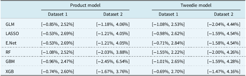


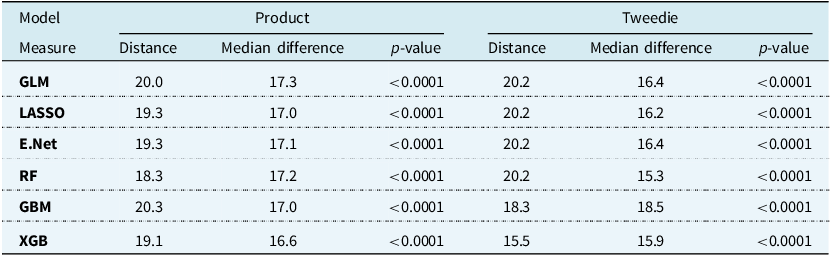


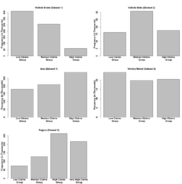

 Open access