


1. Introduction
The Antarctic ice sheet covers about 86% of Earth's glacial area (Aster and Winberry, Reference Aster and Winberry2017). The seismic structures of the Antarctic ice sheet, including P and S wave velocities (v p and v s), v p/v s ratios and ice thicknesses, are important parameters of an ice sheet. Accurate seismic velocity structures and thicknesses of the ice sheets provide key constraints to glacial seismicity and subglacial environment studies (Podolskiy and Walter, Reference Podolskiy and Walter2016; Aster and Winberry, Reference Aster and Winberry2017). The v p/v s ratio, intimately connected to Poisson's ratio, can be used to calculate elastic properties (e.g. bulk modulus and shear modulus) that serve as important parameters in dynamic modeling of ice sheets (Cuffey and Paterson, Reference Cuffey and Paterson2010; Gudmundsson, Reference Gudmundsson2011; Gagliardini and others, Reference Gagliardini2013; Hanna and others, Reference Hanna2013). Exploring effective methods to investigate ice thickness and elastic properties is therefore of inherent scientific interest. Many geophysical methods, including radio-echo sounding (RES) and active seismic methods, have been applied to investigate ice structures over the past half century (Evans and Robin, Reference Evans and Robin1966; Robinson, Reference Robinson1968; Röthlisberger, Reference Röthlisberger1972; Drewry and others, Reference Drewry, Jordan and Jankowski1982; Bamber and others, Reference Bamber, Layberry and Gogineni2001; Gogineni and others, Reference Gogineni2001; Lythe and Vaughan, Reference Lythe and Vaughan2001; Kim and others, Reference Kim2010; Horgan and others, Reference Horgan2011; Fretwell and others, Reference Fretwell2013; Li and others, Reference Li2013). The RES and active seismic methods both are high-accuracy ice thickness detection methods and are sensitive to density and seismic velocity structures, respectively. They both, however, are relatively laborious and costly to implement in Polar regions.
With the rapid development of portable seismic instrumentation in Polar regions, passive seismic methods can also provide a valuable complement to existing methods for interpreting various kinds of seismic signals related to ice dynamics, as well as for resolving glacier and ice-sheet structures (Podolskiy and Walter, Reference Podolskiy and Walter2016; Aster and Winberry, Reference Aster and Winberry2017). Single-station passive seismic methods including P-wave receiver functions (PRFs) and the horizontal-to-vertical spectral ratio (HVSR) provide additional detail of glacier and ice-sheet structures, including ice thickness, ice fabrics and sub-glacial properties. The PRF method applied to teleseismic waveforms, exploiting the converted P-to-S phase and its multiples generated at the interface of a discontinuity, can be used to derive an average depth of the discontinuity and v p/v s ratios with the aid of a stacking H-Kappa (v p/v s) algorithm (Langston, Reference Langston1979; Zhu and Kanamori, Reference Zhu and Kanamori2000). The PRF method has been used to investigate ice thicknesses, ice anisotropic structures and subglacial conditions in polar ice sheets (Anandakrishnan and Winberry, Reference Anandakrishnan and Winberry2004; Hansen and others, Reference Hansen2010; Wittlinger and Farra, Reference Wittlinger and Farra2012, Reference Wittlinger and Farra2015; Chaput and others, Reference Chaput2014; Walter and others, Reference Walter, Chaput and Lüthi2014; Yan and others, Reference Yan2017). By computing the ratio between the horizontal and vertical Fourier spectra of three-component ambient seismic noise or an earthquake record, the HVSR method can quickly retrieve the seismic structures of a medium (Nakamura, Reference Nakamura1989; Lunedei and Malischewsky, Reference Lunedei, Malischewsky and Ansal2015; Bao and others, Reference Bao2018). This method has been increasingly applied in ice environments to study seismic structures of uppermost permafrost, firn, glaciers and ice sheets (Lévêque and others, Reference Lévêque, Maggi and Souriau2010; Picotti and others, Reference Picotti2017; Yan and others, Reference Yan2018; Köhler and Weidle, Reference Köhler and Weidle2019). More recently, Preiswerk and others (Reference Preiswerk2019) have illustrated the effect of geometry of different types of Alpine glaciers on the seismic wavefield and consequently on the retrieved glacier structures using the HVSR method.
Some other passive seismic methods including ambient noise interference and shear wave splitting methods have also be used to estimate seismic structures of ice sheets effectively. Zhan and others (Reference Zhan2014) detected the seismic resonances within the sub-ice water cavity of Amery Ice Shelf using ambient seismic noise cross-correlations. Walter and others (Reference Walter2015) measured phase velocities using ambient seismicity on glaciers and ice sheets. Diez and others (Reference Diez2016) investigated the associated firn/ice/water structure of Ross Ice Shelf with surface-wave dispersion curves. Moreover, the seismic anisotropic structure of ice sheets can also be revealed by passive seismic methods. Harland and others (Reference Harland2013) measured ice anisotropy in Rutford Ice Stream, Antarctica with basal seismicity using the shear-wave splitting method. With more data involved, Smith and others (Reference Smith2017) observed the diffuse horizontal partial girdle fabric in Rutford Ice Stream, which is different from the anisotropic cluster fabric found in other ice streams such as Whillans Ice Stream (Picotti and others, Reference Picotti2015).
Though these results are encouraging, it is still valuable to explore ways to expand the toolbox for glacier and ice-sheet structure detection. Phạm and Tkalčić (Reference Phạm and Tkalčić2017) have proposed a telesismic p-wave coda autocorrelation method, which only uses a single component of seismic records to recover the reflection response from a shallow discontinuity interface (i.e. an ice-bedrock interface). The autocorrelation method together with PRF and HVSR methods that can be applied to ice-sheet structure investigations is all single-station passive seismic methods. The detection abilities of the three methods for retrieving ice-sheet structures in different glacialogical environments such as tilted interfaces and different ice-sediment-bedrock settings have not been analyzed. In this study, the seismic structures, including v p/v s ratios and thicknesses of ice sheets are retrieved beneath 41 stations in East and West Antarctica generally following the autocorrelation method proposed by Phạm and Tkalčić (Reference Phạm and Tkalčić2017). Given that an improved autocorrelation method was also recently applied to a similar set of stations, as in this study (Phạm and Tkalčić, Reference Phạm and Tkalčić2018), we have compared results for stations common to both studies. The consistency of results obtained from independent studies validates the effectiveness of the autocorrelation method. Moreover, comparisons of PRF, HVSR and the autocorrelation methods with their general theories, observed results and theoretical simulations will also be presented in this study.
2. Data and methods
To compare results obtained using PRF, HVSR and autocorrelation methods, we collected data from stations that were commonly processed using PRF and HVSR methods in our previous studies (Yan and others, Reference Yan2017, Reference Yan2018). Specifically, we used data that were recorded by GAMSEIS, and POLENET/ANET seismic arrays that efficiently cover East and West Antarctica (Fig. 1). The criteria for selecting teleseismic events for the autocorrelation technique were generally the same as those in the PRF method; the epicentral azimuth was set between 30 and 90°; at a magnitude greater than 5.5. In total, we picked 978 teleseismic events using this standard from the GAMSEIS and ANET seismic arrays, respectively, during the year 2009 and from 2010 to 2011 (Fig. S1).
Station distribution of the two seismic arrays used in this study. Some stations are aligned in three transects marked with AA′, BB′ and CC′. Ice thickness data are from the Bedmap2 dataset (Fretwell and others, Reference Fretwell2013).

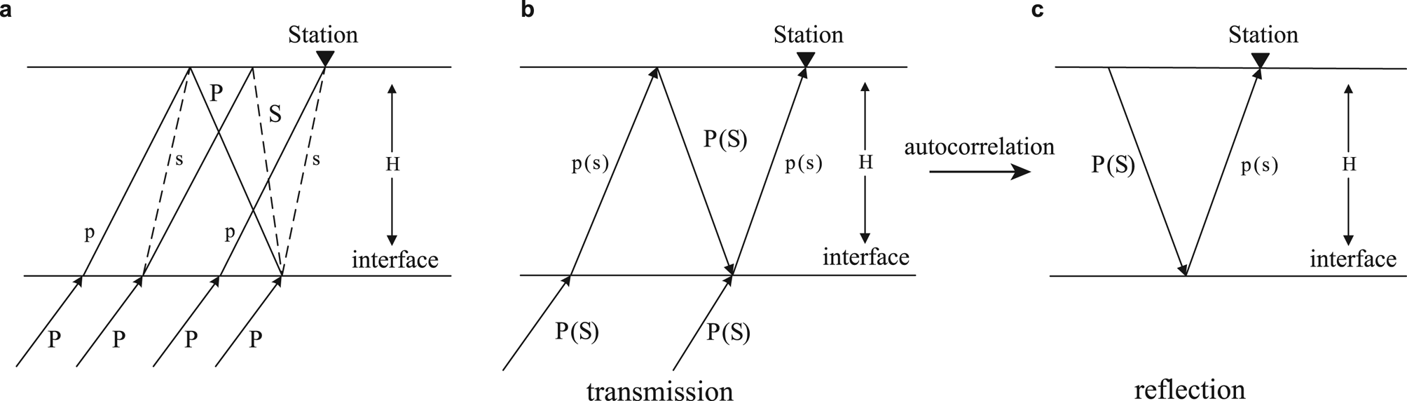
The autocorrelation technique is a seismic interference method for passive seismic imaging which exploits a fast correlation algorithm. The technique was first proposed by Claerbout (Reference Claerbout1968) in a layered acoustic medium. He demonstrated that the autocorrelation of the transmission response of a seismogram generated with a source at depth corresponds to the reflection response of a co-located source and receiver at the surface (Figs 2b and c). This method was extended to a 1-D elastic medium by Frasier (Reference Frasier1970) and later to a 3-D elastic medium by Wapenaar and others (Reference Wapenaar, Thorbecke and Draganov2004). Unlike cross-correlations conducted to retrieve Green's function between station pairs, and often used to extract the surface-wave component (Campillo and Paul, Reference Campillo and Paul2003; Shapiro and Campillo, Reference Shapiro and Campillo2004; Li and others, Reference Li2016), the autocorrelation method can retrieve body-wave reflection responses of discontinuities at different depths by assuming a co-located source and receiver at a single station. Compared with the PRF method that exploits a deconvolution algorithm between radial (or tangential) and vertical components, and the HVSR method that divides vertical and horizontal amplitude spectra, the autocorrelation method uses only one component employing the correlation algorithm.
Sketch of teleseismic phases to compare the PRF and autocorrelation methods. Panel (a) presents the direct P wave, the converted Ps wave and the multiples traveling through an ice-sheet layer used in the PRF method. Panel (b) shows P or S transmissions, while panel (c) shows P or S reflections (modified after Gorbatov and others, Reference Gorbatov, Saygin and Kennett2012). When applied with the autocorrelation technique, the transmitted P wave or S wave is equivalent to reflection waves generated using a co-located source and receiver.
The autocorrelation method has shown its effectiveness when imaging interfaces associated with strong seismic impedance contrasts in Earth crust and upper mantle (e.g. Moho and lithosphere asthenosphere boundary, and the basement of sedimentary basins) (Tibuleac and others, Reference Tibuleac and von Seggern2012; Gorbatov and others, Reference Gorbatov, Saygin and Kennett2012; Kennett, Reference Kennett2015; Kennett and others, Reference Kennett, Saygin and Salmon2015; Saygin and others, Reference Saygin, Cummins and Lumley2017) and seismic interfaces on the moon (Nishitsuji and others, Reference Nishitsuji2016). In most previous studies, the autocorrelation method is applied to ambient noise data. When applied to ambient noise data, a large amount of noise data is required to enhance the signal-to-noise ratio (SNR) and the stability of results. The autocorrelation technique applied to teleseismic events has recently been validated as effective for mapping reflection responses of interfaces at both deep and shallow depths (Sun and Kennett, Reference Sun and Kennett2016, Reference Sun and Kennett2017; Phạm and Tkalčić, Reference Phạm and Tkalčić2017). The use of teleseismic events has advantages, including less-strict requirements for data volume and processing procedures that are simpler than those required with ambient noise data.
Processing procedures in the autocorrelation method generally include pre-processing, such as data-quality control and whitening, autocorrelation in time or frequency domains and post-processing such as filtering and stacking. In this study, we computed autocorrelograms in the frequency domain, which is more efficient than processing in the time domain (since a deconvolution procedure required in the time domain is equivalent to a simple division in the frequency domain). Pre-processing procedures were conducted including the removal of the mean and linear trend. A whiten operation was applied to the pre-processed waveforms so as to enhance the high frequency signals that attenuated when propagating along the ray path. In contrast to Phạm and Tkalčić (Reference Phạm and Tkalčić2018), which improved the autocorrelation method by using a station-specific tuning whiten width, we adopted a fixed one in this procedure and achieved similar results. The adoption of a fixed whiten width is more suitable for automatic processing, especially for seismic arrays. Autocorrelograms were calculated in the frequency domain, and the positive time lags of a symmetric autocorrelogram were retained. A cosine taper function was applied to remove the inherent zero-time peak in the retained autocorrelogram. To recover coherent reflection responses of the ice-sheet-rock interface in both vertical and radial components, several sets of Butterworth bandpass filters were tested on the retained autocorrelogram. A final 0.5–2 Hz frequency band was adopted as it presented the clearest reflection responses (Fig. S2). Retained time series data were normalized using the maximum amplitude. To enhance the reflection response from the ice-bedrock interface, the autocorrelograms of all teleseismic events recorded at one station were stacked using the time-frequency domain phase weighted stacking (TF-PWS) technique (Schimmel and Gallart, Reference Schimmel and Gallart2007). Following a previous study, the PWS order that we adopted in the stacking procedure is 2 (Pham and Tkalčić, Reference Phạm and Tkalčić2017).
Theoretical autocorrelograms using synthetic teleseismic waveforms were also calculated to validate the observed autocorrelograms for each station. The synthetic teleseismic waveforms were computed via convolution of a source time function and an impulse response of a local structure (Fig. 3a). Unlike the source time function adopted by Pham and Tkalčić (Reference Phạm and Tkalčić2017), which is comprised of an array of normally distributed random numbers with mean 0 and Std dev. 1 (Fig. 3b), we use 100 real teleseismic waveforms in the vertical component, each lasting 12 s to represent the real source time function (Fig. 3c). The use of a real vertical teleseismic waveform as a source time function has advantages over that adopted by Pham and Tkalčić (Reference Phạm and Tkalčić2017) as it uses the real source and involves the effect of ray paths, making the synthetic teleseismic waveforms more similar to the real ones. The local structure impulse response was calculated using the reflection program (repknt, Randall, Reference Randall1989), assuming a homogeneous and isotropic ice-sheet layer atop hard bedrock. The parameters including ice thickness and P and S wave velocities used in models to generate local impulses are derived from the Bedmap2 dataset and previous studies (Hansen and others, Reference Hansen2010; Wittlinger and Farra, Reference Wittlinger and Farra2012; Ramirez and others, Reference Ramirez2016). Given that the thickness of ice sheets is much thinner, <4 km, than that of crustal and mantle discontinuities, the reflection delay times of the ice-bedrock interfaces are independent of ray parameters (Pham and Tkalčić, Reference Phạm and Tkalčić2017). We therefore calculated the local impulse responses at fixed slowness, 0.06 s km–1, for the P wave, and 0.12 s km–1, for the S wave (Sun and Kennett, Reference Sun and Kennett2016) (Figs 3f and g). The subsequent processing procedures to generate theoretical autocorrelograms using synthetic teleseismic waveforms remain the same as those applied to real teleseismic P wave coda waveforms.
Example of synthetic teleseismic waveforms generated using different source time functions and the radial and the vertical autocorrelograms before and after TF-PWS stacking for station GM01. Panel (a), v p and v s profiles for station GM01 with a 3.1 km thick ice layer. Panel (b), from top to bottom: a source time function similar to that adopted by Pham and Tkalčić (Reference Phạm and Tkalčić2017), is comprised of an array of normally distributed random numbers with mean 0 and Std dev. 1, a local structure impulse response, a complete teleseismic waveform. Panel (c), the same as panel (b) except the source time function is a segment of a real vertical teleseismic waveform. Panels (d) and (e), the synthetic vertical and radial autocorrelograms generated using the source time function shown in panel (b). Panels (f) and (g), the synthetic vertical and radial autocorrelograms generated using 100 source time functions as shown in panel (c).

3. Results
High quality vertical autocorrelograms were obtained for all 41 stations; 39 were obtained for the radial component, because there were no clear reflection responses or too few high quality autocorrelograms at stations ST04 and ST06 (Fig. S3). The stacked autocorrelograms in both the vertical and the radial components for the 39 stations are displayed in Fig. 4. Comparisons of the autocorrelograms before and after stacking show that the PWS technique enhances the coherent phases and suppresses incoherent phases, thus improving the SNR of the autocorrelograms.
Stacked radial and vertical autocorrelograms of 39 stations. Panel (a), the stacked vertical autocorrelograms (ZAC). Yellow circles represent the arrival times of P wave reflection responses, and blue circles denote arrival times that double the values of the first P wave reflection arrival times. Panel (b), the same as panel (a), but for the radial autocorrelograms and S wave reflection responses. Panel (c), v p/v s ratio values derived from the ratios of S wave and P wave reflections obtained from this study and Pham and Tkalčić (Reference Phạm and Tkalčić2018). The v p/v s ratio estimates obtained from the PRF method are also shown in panel (c) (Yan and others, Reference Yan2017).
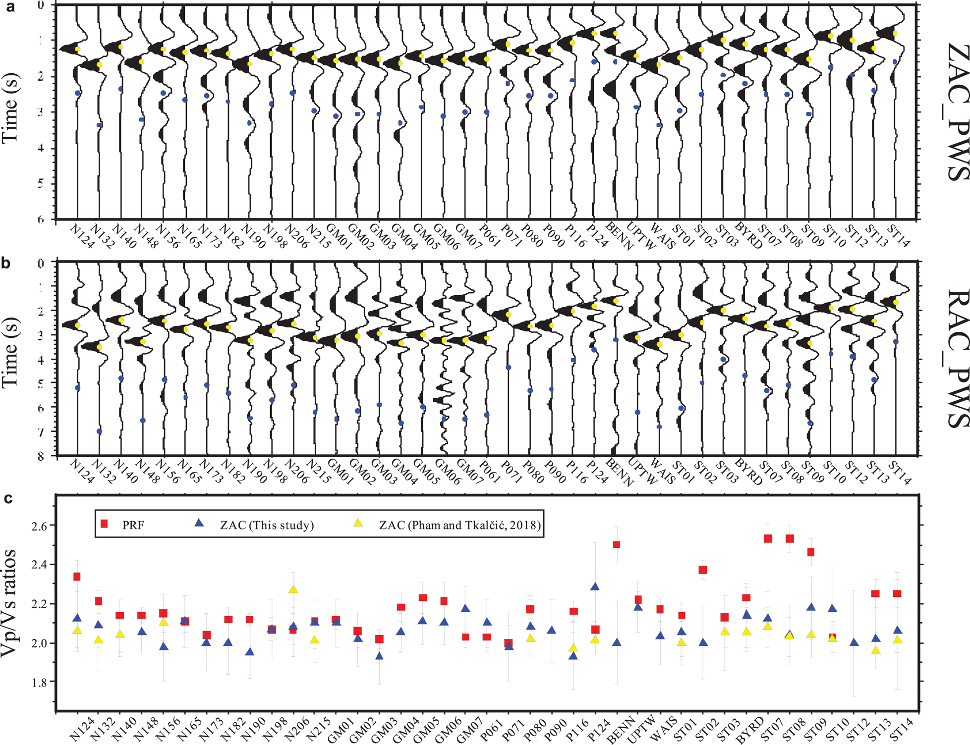
As shown in Figs. 4a and b, there are clear dominant and negative peaks for each autocorrelogram in both the vertical and the radial components. The arrival times show significant variations between different stations, reflecting the variations of ice thicknesses beneath these stations. An examination of the arrival times of the negative peaks in the vertical component reveals that peaks appear in the 0.80–1.68 s range, while the arrival times of the radial peaks are approximately double those for the vertical peaks (i.e. 1.60–3.40 s). The negative peaks are the first P or S reflection responses of the ice-bedrock interface. The first reflection responses show negative polarities because the first reflection experiences a single phase flip due to a single reflection of the free surface (Pham and Tkalčić, Reference Phạm and Tkalčić2017). Moreover, clear positive peaks appear at twice the time of the first P (S) reflection responses for most stations, which are certainly the second reflections. These peaks show positive polarities because they experience twice the free surface reflections, thus their travel times are generally double those of the first reflections. The second reflection responses are generally much weaker or even invisible for some stations (e.g. N148, GM03 and ST10) because the seismic energy attenuates during subsequent propagation in ice. We then define the arrival times for the P and S waves (t p and t s) to be the times at which the peaks of the maximum amplitudes occur. The chosen arrival times are associated with uncertainties that arise from the TF-PWS stacking and the maximum amplitude identification. In this sense, we estimate the uncertainties (δt p and δt s) using the difference in arrival times between the peak amplitude and ${\sqrt2/2}$ times the peak amplitude. The P and the S wave arrival times, as well as their associated uncertainties are listed in Table 1.
Arrival times of the reflection responses for the P and S waves, and the calculated v p/v s and Poisson's ratios
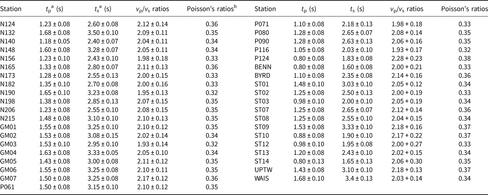
a The uncertainty of the arrival times for the P and the S waves is estimated using the difference in the arrival times between the peak amplitude and ${\sqrt2/2}$ times the peak amplitude.
b $\upsilon = \displaystyle{{{\lpar {v_{\rm p}/v_{\rm s}} \rpar }^2-2} \over {2{\lpar {v_{\rm p}/v_{\rm s}} \rpar }^2-2}}$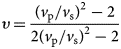
Having identified the arrival times of P and S wave reflection responses, we calculate the value of the v p/v s ratio for each station. The v p/v s ratio is proportional to the ratio between the S and the P wave arrival times as their ray paths are both near vertical traveling through the ice sheet; that is

where t p and t s are the arrival times of P and S wave reflection responses, respectively. Using the uncertainties of the P and the S wave arrival times, we calculate the errors of the v p/v s ratios from the error propagation law

where δt p and δt s are uncertainties calculated using the difference in the arrival times between the peak amplitude and ${\sqrt2/2}$ times the peak amplitude. As shown in Fig. 4c, the values of v p/v s ratios are generally in the range of 1.95–2.20 for most stations (Table 1). The minimum and the maximum values of the v p/v s ratios are 1.93 for GM03 and P116 stations and 2.28 for P124 station, respectively. The average value of v p/v s ratios for the 39 stations is 2.07. The results are consistent with the values deduced from laboratory measurements of v p and v s in a single ice crystal; i.e. the values of v p/v s ratios along and perpendicular to the c-axis direction are respectively, 2.14 and 1.97 (Gagnon and others, Reference Gagnon1988).
In addition, the ice-bedrock depths (ice thicknesses) can also be computed using the reflection arrival time and the corresponding seismic velocity of a particular component (vertical or radial). Given that the quality of the vertical autocorrelograms is better than that of the radial ones (there are phase-interfering S wave reflection responses in radial autocorrelograms as shown in Fig. 4b), we use the velocity and reflection arrival times in the vertical component to calculate the ice thickness; that is,

Neglecting the variations of ice parameters at different sites, a homogeneous v p value (3800 m s–1) was adopted in our study, which was determined using a reflection seismic method and was widely used in relevant studies (Robinson, Reference Robinson1968; Röthlisberger, Reference Röthlisberger1972). The uncertainty of P wave velocity (δv p) is set to 100 m s–1 considering the influence of temperature and anisotropy on ice elastic properties (Kohnen, Reference Kohnen1974). Errors from the picked arrival time of the P wave reflection response and from the P wave velocity both contribute to the uncertainty of the estimated ice thickness. Note that the calculated ice thickness would be slightly larger than the ‘ground truth’ ice thickness as the P wave velocity in the uncompacted firn near the surface is smaller than that in the deeper ice (the associated error however can be neglected as the seismic velocity quickly reaches 3800 m s–1, Robinson, Reference Robinson1968; Röthlisberger, Reference Röthlisberger1972). Hereafter we define the ice thickness estimates obtained from the autocorrelograms using the P reflection responses as ZAC estimates. The computed ice thicknesses and the associated uncertainties (Eqn (4)) are listed in Table S1.

4. Discussion
The stacked theoretical autocorrelograms together with the Bedmap2 ice thickness variations across three profiles are shown in Figs 5 and S5. There is good agreement between the observed and the theoretical arrivals of the reflection responses for most stations. The relative errors of the observed first P wave reflections to the theoretical ones are within 5, 10 and 15% at a total of 19, 27 and 32 stations, respectively. Similarly, the relative errors for S wave reflections for 17, 27 and 29 stations are within 5, 10 and 15% threshold, respectively. In addition, the variations between the Bedmap2 ice thicknesses and the reflection arrivals for stations along the three profiles are closely correlated. Given that the Bedmap2 ice thicknesses adopted to generate theoretical teleseismic waveforms are associated with certain uncertainties at these stations (Fretwell and others, Reference Fretwell2013; Yan and others, Reference Yan2018), we can conclude that the autocorrelation method can effectively image both the P wave and the S wave reflection responses of the ice-bedrock interface.
Synthetic stacked radial and vertical autocorrelograms for each station. Panel (a) shows Bedmap2 ice thickness variations along the three profiles and the reference thicknesses (red dots) used to build models. Panel (b) displays synthetic vertical autocorrelograms. Yellow and blue crosses denote the arrival times of the observed first and second P wave reflection responses (corresponding to the yellow and blue circles shown in Fig. 4a). Panel (c) is similar to panel (b), but for radial autocorrelograms. Model parameters used to generate theoretical teleseismic waveforms are comprised of Bedmap2 ice thickness, v p and v s values. v p is set to 3800 m s–1 referring to previous studies and v s is deduced from the relationship between v p and v p/v s ratio.

Given the lack of ‘ground truth’ ice thickness from direct measurement methods such as drillings, calculated ice thickness is validated by comparing the ZAC estimate with the corresponding Bedmap2 ice thickness at each site. Differences between the ZAC estimates and the Bedmap2 ice thickness are within 100, 200, 300 and 400 m for 15, 24, 29 and 33 stations, respectively. The relative errors of the ZAC estimates to the Bedmap2 ice thickness are the same as those of the observed arrival times to the theoretical arrival times because the same v p value is used in calculations of ice thicknesses and models to generate theoretical autocorrelograms. Our estimates show a good agreement with results obtained from Pham and Tkalčić (Reference Phạm and Tkalčić2018), which investigated Antarctic ice-sheet properties using an autocorrelation method with an improved scheme of selecting the spectral whiten width. Comparison shows, for the 19, 27 and 33 out of 38 stations that exhibit clear P wave reflections in both studies, the relative errors are within 5, 10 and 15%, respectively (Fig. 6). Note that instead of using ice thickness results estimated by Pham and Tkalčić (Reference Phạm and Tkalčić2018) directly, we adopt their P wave arrival times and use the same P wave velocity value as in our study to calculate ice thicknesses since different v p values were used in two studies. Though the relative errors of ice thickness at stations P061 and N190 appear over 50% (Fig. 6), we find that the arrival times are shown in autocorrelograms in Pham and Tkalčić (Reference Phạm and Tkalčić2018) and our studies are in fact very close. The differences are caused by their recording mistakes as the arrival time values recorded in the table are not consistent with the ones shown in the autocorrelograms (Pham and Tkalčić, Reference Phạm and Tkalčić2018).
Comparison of the ZAC ice thickness estimates with results obtained using the HVSR and PRF methods in our previous studies (Yan and others, Reference Yan2017, Reference Yan2018). The grey horizontal line in the plot indicates the average ice thickness of the HVSR, PRF and ZAC (this study) estimates for each station. The red circle and its bar represent the Bedmap2 ice thickness and its associated uncertainty for each station (Fretwell and others, Reference Fretwell2013). The ZAC estimates measured by Pham and Tkalčić (ZAC) are also displayed here (yellow stars) (note that the thickness values are a product of P wave arrival times taken from Pham and Tkalčić (Reference Phạm and Tkalčić2018) and v p adopted in this study; we don't use their ice thickness values as two slightly different v p values are used in different studies).

As no comparison among ice thickness estimates obtained from the PRF, HVSR and autocorrelation methods has been conducted before, we compared the ZAC estimates with results derived from the PRF and HVSR methods in our previous studies (Yan and others, Reference Yan2017, Reference Yan2018). We have calculated the average ice thickness at the 35 stations that successfully acquire ice thickness estimates using the PRF, HVSR and autocorrelation methods simultaneously. It shows that the ice thickness estimates obtained from the three methods are consistent as the differences of ice thickness values estimated by each method from the average of their ice thickness values are within 200 m at ~30 stations. Table S2 displays the relative errors of the ice thickness estimates with respect to the Bedmap2 ice thickness. We find that the level of relative error in the estimates is also consistent – the relative errors are within 15% for 25 stations, including GM01, P061, BYRD and ST01. This consistency can also be found for the seven stations with relatively large relative errors to the Bedmap2 ice thicknesses (over 15%), such as the N206, GM03 and ST09 stations. Similar disagreements with Bedmap2 ice thicknesses at these stations have also been found by Pham and Tkalčić (Reference Phạm and Tkalčić2018).
It is possible that the relatively large deviations from Bedmap2 ice thicknesses at the seven stations could be attributed to uncertainties in Bedmap2 ice thicknesses. More accurate ice thicknesses could be required to validate these specific results. The deviations could also be caused by the complex subglacial settings beneath these stations. As pointed out by Chaput and others (Reference Chaput2014), it is difficult to model the converted phases from the base of the ice sheet in their PRF study for a few stations including ST04, ST06 and ST09, which could possibly be influenced by anisotropy or basal dip structures. Therefore, we calculated autocorrelograms using synthetic teleseismic waveforms derived from models assuming an ice-sheet layer atop an inclined bedrock layer with dip angles varying from 5 to 30°, to show the effect of nonplanar basal topography on autocorrelograms. Figure S6 shows the theoretical teleseismic waveforms with a range of back azimuths between 0 and 360° generated using the raysum codes (Frederiksen and Bostock, 2000). Figure S7 displays the resulting autocorrelograms obtained using the theoretical teleseismic waveforms with the processing strategies mentioned in section 2. We can find that the autocorrelation reflections from different back azimuths show clear variations in values of amplitudes and arrival times. Such features become more remarkable as the dip angle increases. For example, the arrival time of the vertical autocorrelation reflections shown in the left panel of Fig. S7 decreases from 1.55 to 1.40 s when the dip angle increases from 5 to 15°. In addition to decreasing arrival times, the autocorrelations become more complex when the dip angle exceeds 20°. The same characteristics can also be found in radial autocorrelograms. With the PWS technique applied, we found that the azimuthal effect on the autocorrelograms resulting from the inclined basal structures is suppressed as a consistent autocorrelation reflection from different back azimuths is obtained (Fig. S8). Arrival times identified from the consistent autocorrelograms only reflect an average ice thickness beneath a station. Therefore, basal dips could certainly affect the arrival times of P and S wave reflection responses and consequently lead to errors of ice thickness estimates (and v p/v s ratios).
The PRF and the autocorrelation methods share certain similarities in data selection criteria and in the underlying equations in the frequency domain


where P(ω) and S(ω) are the vertical and radial component spectra from teleseisms at angular frequency ω, and P*(ω) is the complex conjugation of P(ω) (Sun and Kennett, Reference Sun and Kennett2016). The water level parameter c in Eqn (6) is used to avoid division by very small numbers by reducing the magnitude of the trough in the vertical component spectrum (Clayton and Wiggins, Reference Clayton and Wiggins1976). For small c, Eqn (6) approaches deconvolution, while it approaches a scaled cross-correlation as c becomes large. Considering the similarities of the PRF and autocorrelation methods, we compare their results for ice thickness and v p/v s ratios. It turns out that ice thickness estimates obtained from the PRF and autocorrelation methods are closely matched (for the total of 38 stations that are common to both methods, the relative error of the ZAC estimates to the PRF estimates for 22 and 34 station are less than 5 and 10%, respectively). Taking the uncertainties in the estimated v p/v s ratios into account, the values of v p/v s ratios determined using PRF and autocorrelation methods are generally consistent and ~2.00 for most stations (see Fig 4c). The differences are less than 0.1 for 17 stations, while the differences for stations such as BENN, ST02, ST07 and ST08 exceed 0.35. Further analysis indicates that the quality of PRF waveforms used to conduct H-Kappa stacking (Zhu and Kanamori, Reference Zhu and Kanamori2000) for the four stations is poorer than that of the autocorrelograms (Fig. S4). As is commonly acknowledged, the inherent trade-off between the thickness and shear-wave velocity for the PRF method also contributes to uncertainties in the v p/v s estimates.
To clearly show the capacity of the two methods for detecting ice properties, we have built a set of models (Fig. S10) to compare results obtained from both PRF and autocorrelation methods (Anandakrishnan and Winberry, Reference Anandakrishnan and Winberry2004; Chaput and others, Reference Chaput2014). Conclusions can be drawn by comparing results using different pairs of models (Figs 7, 8 and S11–S13). Table S1 displays the theoretical arrival times of P and S wave reflection responses calculated from model parameters (Eqns (7–9)), as well as the observed arrival times derived from the synthetic autocorrelograms using a bootstrapping technique (Fig. S14).


where H ice and H sed are ice and sediment thicknesses, and $t_{{\rm p(s)}}^{{\rm ice}}$ , $t_{{\rm p(s)}}^{{\rm ice + sed}}$
 are the theoretical arrival times of P (S) wave reflection responses in ice, and in ice and sediment layers. v p(s) is P (S) wave velocities in ice, and $\bar{v}_{{\rm p(s)}}$
 is the weighted average P (S) wave velocities in ice and sediment layers. Figure 7 shows the results obtained from model 1 and model 2 assuming two ice-sheet layers with different values of v p/v s ratios. It is clear that the ice thickness and v p/v s ratio estimates obtained from the PRF and H-Kappa methods are closer to the theoretical values than those obtained from the autocorrelation method (Fig. 7). The deviations of the theoretical v p/v s ratios from the estimated ones are attributed to the differences between the theoretical and the observed P and S wave arrival times. For example, the theoretical P wave and S wave reflection arrival times of model 1 are 1.55 and 2.94 s, while the observed values are 1.4 and 2.83 s (Table S1). Figures 8 and S11 show that both the autocorrelograms and the PRF waveforms become complicated when sedimentary layers are involved. The H-Kappa technique failed to acquire optimum estimates of ice thickness and v p/v s ratios using PRF waveforms as the phases from the sediment-bedrock interface greatly obscure phases from the ice-sediment interface (Figs S11–S13). A comparison of the theoretical and the observed arrival times of P or S wave reflection responses indicates that the autocorrelation method can only identify interfaces associated with strong impedance contrasts (Table S1). For example, Figure S10 shows that the P wave impedance contrasts (z = ρ · v p, where z is the impedance contrast, and ρ and v p are density and P wave velocity of the medium) set at the sediment-bedrock interfaces for models 4 and 6 are stronger than those set at the ice-sediment interfaces for models 3 and 5. Consequently, the observed P wave arrival times identified from models 3 (2.32 s) and 5 (2.35 s) are (nearly) equal to the theoretical times that were calculated with both the ice sheet and the sediment layers included (2.35 s for models 3 and 5). By contrast, the observed P wave arrival times of models 4 (1.46 s) and 6 (1.50 s) correspond to the theoretical times calculated with the single ice sheet layer (1.55 s). Similar results can be found for radial components (Table S1). Comparing results for models 3 and 4, we can find that the observed S wave arrival time of model 3 (4.73 s) is close to the theoretical arrival time (4.46 s) calculated including both the ice sheet and the sediment layers, while the observed arrival time of model 4 (2.77 s) approaches the theoretical arrival time (2.94 s) with the ice-sheet layer alone. We can also find that the observed S wave arrival time of model 6 (3.38 s) corresponds to the theoretical arrival time with the single ice-sheet layer (3.45 s) as the v s value in ice decreases from 2.04 km s–1 in model 4 to 1.74 km s–1 in model 6, thus increasing the impedance contrast at the ice-sediment interface. Pham and Tkalčić (Reference Phạm and Tkalčić2018) pointed out that the low velocity of sediment results in low impedance contrast, explaining the relative transparency of sediment below an ice-sheet layer. In this sense, the autocorrelation method should be applied with caution to study low velocity sediment layers in glaciological settings. Alternatively, a nonlinear inversion method that is similar to the PRF waveform inversion approach could be effective to obtain the optimum model that fits with the observations.
Estimates of v p/v s ratios obtained from the PRF and autocorrelation methods using theoretical teleseimic waveforms based on models 1 and 2 (panels (a) and (e)). Panels (b), (c) and (d) show the stacked autocorrelograms, PRF waveforms and H-Kappa results for model 1, and the right panels display results for model 2. The arrival times used to calculate v p/v s ratios in panels (b) and (d) are automatically picked using the bootstrapping technique (Koch, Reference Koch1992) shown in Fig. S14. The v p/v s ratio estimate obtained from PRF and H-Kappa methods is closer to the theoretical value than that measured using the autocorrelation method.

Effect of a sediment layer (model 3) on v p/v s estimates obtained from the PRF and autocorrelation methods. Panels (b), (c) and (d) present the stacked autocorrelograms, PRF waveforms and the H-Kappa results for model 1, and the right panels show results for model 3. This comparison illustrates that neither the PRF method nor the autocorrelation method can clearly identify the ice-sediment interface (Table S1). The estimated v p/v s ratios obtained from the PRF and autocorrelation methods also deviate from the theoretical values.

The modeling results do not suggest that the autocorrelation method is superior to the PRF method, but it is still an effective alternative to the PRF method as it only requires a single component, which expands its application to datasets that were collected using single-component sensor decades ago. Moreover, the autocorrelation method can constrain both P wave and S wave velocity structures independently if both vertical and radial component records are available, while the PRF method can only reveal S wave velocity profiles. It is worth mentioning that there is a promising way to better constrain the thickness, v p and v s of an ice-sheet layer as a recent study has proposed a new H-Kappa-v p stacking algorithm, which exploits independent constraints from the P wave autocorrelation and receiver functions (Delph and others, Reference Delph, Levander and Niu2019).
Unlike the close relationship between the PRF and autocorrelation methods, there are more differences than similarities between the HVSR method and the autocorrelation method. First of all, seismic ambient noise data are usually adopted for HVSR processing, though earthquake records can also be used. Secondly, the spectrum peak observed by the HVSR method represents S wave resonance frequency and only reflects S wave energy trapped in a medium, while the autocorrelation method can reveal P and S wave energy separately. Both the autocorrelation and PRF methods require a certain number of teleseismic earthquakes, and such data usually take a relatively long time to collect in Antarctica. By contrast, the HVSR method applied to ambient noise records only requires a recording time of several hours, making it a valuable complement to the autocorrelation and PRF methods (Yan and others, Reference Yan2018). Furthermore, the HVSR method combined with an inversion algorithm can be used to reveal inner stratification structures of ice sheets (Yan and others, Reference Yan2018), which the autocorrelation method has failed to detect (Pham and Tkalčić, Reference Phạm and Tkalčić2017).
As the v p/v s ratio is closely related to Poisson's ratio, we also calculated Poisson's ratio at each station using the relation shown in Eqn (10) (Christensen, Reference Christensen1996). The computed Poisson's ratios range from 0.32 to 0.38 (Table 1) and the average value (0.35) is slightly higher than the fixed value 0.33 used in previous studies (Gudmundsson, Reference Gudmundsson2011; Rosier and others, Reference Rosier, Gudmundsson and Green2015; Ramirez and others, Reference Ramirez2016).

Variations in the value of Poisson's ratio at different sites could be attributed to temperature differences in different regions. Thus, rather than using a constant value for Poisson's ratio, it is more reasonable to consider a variable Poisson's ratio for large-scale ice-sheet modeling.
5. Conclusions
Estimates of ice thickness and v p/v s ratios at 39 stations of the GAMSEIS and the ANET seismic arrays in Antarctica have been obtained using the recently proposed autocorrelation method. Results derived from the autocorrelation method were validated with synthetic tests at each station and compared with those derived from two other single-station passive seismic methods (i.e. the PRF and HVSR methods). The values of v p/v s ratios obtained in this study are within the range of experimental measurements. The spatial variations of elastic properties (e.g. Poisson's ratios deduced from v p/v s ratios) of ice sheets should be considered in large-scale modeling of ice-sheet dynamics. Consistent estimates of ice thickness are found among the PRF, HVSR and autocorrelation methods. Comparisons conducted under various model setups show the effectiveness of the autocorrelation method is not superior to the PRF method for retrieving seismic structures of ice sheets. However, the use of seismic records of a single component seismometer expands its application to datasets collected using only one-component sensors. It also opens a way to constrain P wave and S wave velocity profiles separately. However, in cases where the PRF and autocorrelation methods cannot be used due to a short time record of seismic data, the HVSR method can be a valuable tool for ice-sheet structure detection.
Acknowledgement
We thank the editor and reviewers for their constructive comments that greatly improved the manuscript. This work was supported by the State Key Program of National Natural Science of China under Grant 41531069, NSFC41476163, NSFC41674065, CAST-BISEE Foundation and the Chinese Polar Environment Comprehensive Investigation and Assessment Programs under Grant CHINARE2017-02-03. Seismic data used in this study are obtained from the Incorporated Research Institutions for Seismology (IRIS). Figures in this study were plotted using Generic Mapping Tools (GMT).
Supplementary material
The supplementary material for this article can be found at https://doi.org/10.1017/jog.2019.95


 Open access