


1. Introduction and motivation
Given independent random variables X and Y, the study of the stochastic monotonicity of each marginal given the value of their sum $S=X+Y$
(that is,
$S=X+Y$
(that is, $X\mid S=s_1\leq_{st} X\mid S=s_2$
for
$X\mid S=s_1\leq_{st} X\mid S=s_2$
for $s_1\leq s_2$
where
$s_1\leq s_2$
where $\leq_{st}$
represents the usual stochastic order) is usually referred to as “Efron’s monotonicity property” after Efron (Reference Efron1965). In this paper, it was proved that a sufficient condition for X and Y to be stochastically increasing in S is that the summands X and Y possess log-concave densities. However, this assumption might be too strong in certain applications, as log-concave densities are associated with light-tailed asymptotic behavior, as discussed in see Asmussen and Lehtomaa (Reference Asmussen and Lehtomaa2017). Hence, this paper aims to study the implications of considering heavy-tailed random variables.
$\leq_{st}$
represents the usual stochastic order) is usually referred to as “Efron’s monotonicity property” after Efron (Reference Efron1965). In this paper, it was proved that a sufficient condition for X and Y to be stochastically increasing in S is that the summands X and Y possess log-concave densities. However, this assumption might be too strong in certain applications, as log-concave densities are associated with light-tailed asymptotic behavior, as discussed in see Asmussen and Lehtomaa (Reference Asmussen and Lehtomaa2017). Hence, this paper aims to study the implications of considering heavy-tailed random variables.
Let $m_{X}(\!\cdot\!)$
denote the conditional expectation of X given the sum S, defined by
$m_{X}(\!\cdot\!)$
denote the conditional expectation of X given the sum S, defined by
 \begin{equation*}m_{X}(s)=\mathrm{E}[X|S=s].\end{equation*}
The monotonicity of $m_{X}(\!\cdot\!)$
, known as regression dependence, is weaker than Efron’s monotonicity. Therefore, this paper delves into how heavy tailedness affects the monotonicity of
$m_{X}(\!\cdot\!)$
, known as regression dependence, is weaker than Efron’s monotonicity. Therefore, this paper delves into how heavy tailedness affects the monotonicity of $m_{X}(\!\cdot\!)$
. Regression dependence plays an important role in various contexts, as discussed next.
$m_{X}(\!\cdot\!)$
. Regression dependence plays an important role in various contexts, as discussed next.
Within the framework of Peer-to-Peer (P2P) insurance, where risk-holders pool their resources to collectively protect against the financial impact of a given threat, the study of risk-sharing rules is essential. Consider, for instance, two economic agents with respective insurance losses modeled as independent random variables X and Y, who decide to form a pool to share the total loss $S=X+Y$
. Thus, once the peril occurs, each agent pays an ex-post contribution to the pool. These contributions must verify that their sum matches the aggregate loss of the pool. As proposed in Denuit and Dhaene (Reference Denuit and Dhaene2012), the conditional expectations
$S=X+Y$
. Thus, once the peril occurs, each agent pays an ex-post contribution to the pool. These contributions must verify that their sum matches the aggregate loss of the pool. As proposed in Denuit and Dhaene (Reference Denuit and Dhaene2012), the conditional expectations $m_{X}(\!\cdot\!)$
and
$m_{X}(\!\cdot\!)$
and $m_{Y}(\!\cdot\!)$
may be used by participants to distribute the total loss among them. The conditional mean risk-sharing rule has been axiomatized by Jiao et al. (Reference Jiao, Kou, Liu and Wang2022). If
$m_{Y}(\!\cdot\!)$
may be used by participants to distribute the total loss among them. The conditional mean risk-sharing rule has been axiomatized by Jiao et al. (Reference Jiao, Kou, Liu and Wang2022). If $m_{X}(\!\cdot\!)$
decreases over a range of values, then the participant bringing loss X may be tempted to exaggerate the loss, since this would decrease his or her contribution to the pool. Non-decreasingness of
$m_{X}(\!\cdot\!)$
decreases over a range of values, then the participant bringing loss X may be tempted to exaggerate the loss, since this would decrease his or her contribution to the pool. Non-decreasingness of $m_{X}(\!\cdot\!)$
thus appears to be a reasonable and useful requirement in the context of risk sharing, where this property is referred to as the no-sabotage condition.
$m_{X}(\!\cdot\!)$
thus appears to be a reasonable and useful requirement in the context of risk sharing, where this property is referred to as the no-sabotage condition.
The results derived in this paper are also useful in the context of capital allocation. Note that the difference between risk sharing and capital allocation is subtle, and both mechanisms are intimately related. As explained above, risk-sharing consists of distributing a random aggregate loss among the agents in the pool by means of ex-post contributions. That is, once the financial loss occurs, the total loss is calculated and then shared among participants. On the other hand, capital allocation refers to distributing a deterministic aggregate capital. For instance, if a corporation has two lines of business with respective losses X, Y, a capital allocation principle determines $K_X,K_Y\in \mathbb{R}$
with aggregate capital
$K_X,K_Y\in \mathbb{R}$
with aggregate capital $K=K_X+K_Y$
. One popular form to decide the aggregate capital is to consider distortion risk measures. Consider an increasing concave distortion function
$K=K_X+K_Y$
. One popular form to decide the aggregate capital is to consider distortion risk measures. Consider an increasing concave distortion function $g:[0,1]\to [0,1]$
with
$g:[0,1]\to [0,1]$
with $g(0) = 0$
and
$g(0) = 0$
and $g(1) = 1$
. The associated distortion risk measure
$g(1) = 1$
. The associated distortion risk measure $\rho$
is defined such that, for a non-negative random variable Z,
$\rho$
is defined such that, for a non-negative random variable Z, $\rho(Z)=\mathrm{E}[Z g'(\bar{F}_Z(Z))],$
where
$\rho(Z)=\mathrm{E}[Z g'(\bar{F}_Z(Z))],$
where $\bar{F}_Z(\!\cdot\!)$
is the survival function of Z (see Dhaene et al., Reference Dhaene, Kukush, Linders and Tang2012 for further detail). Then, the aggregate capital considered is
$\bar{F}_Z(\!\cdot\!)$
is the survival function of Z (see Dhaene et al., Reference Dhaene, Kukush, Linders and Tang2012 for further detail). Then, the aggregate capital considered is $K=\rho(S)$
with
$K=\rho(S)$
with $S=X+Y$
(see Denault, Reference Denault2001; Tsanakas and Barnett, Reference Tsanakas and Barnett2003 and Chapter 10 in Mildenhall and Major, Reference Mildenhall and Major2022), that is, for continuous losses and distortion,
$S=X+Y$
(see Denault, Reference Denault2001; Tsanakas and Barnett, Reference Tsanakas and Barnett2003 and Chapter 10 in Mildenhall and Major, Reference Mildenhall and Major2022), that is, for continuous losses and distortion, $K=\mathrm{E}[S\;h(S)]$
, where
$K=\mathrm{E}[S\;h(S)]$
, where $h(s)=g^\prime(\bar{F}_S(s))$
. Hence, a natural allocation principle is to determine
$h(s)=g^\prime(\bar{F}_S(s))$
. Hence, a natural allocation principle is to determine $K_X=\mathrm{E}[X h(S)]$
and
$K_X=\mathrm{E}[X h(S)]$
and $K_Y=\mathrm{E}[Y h(S)]$
(see Sections 2 and 3 in Major and Mildenhall, Reference Major and Mildenhall2020 for further details). Since
$K_Y=\mathrm{E}[Y h(S)]$
(see Sections 2 and 3 in Major and Mildenhall, Reference Major and Mildenhall2020 for further details). Since $\mathrm{E}[X h(S)]=\mathrm{E}[\mathrm{E}[X h(S)|S] ]=\mathrm{E}[m_X(S) h(S)]$
, the conditional expectation provides a great simplification, reducing the allocation to a one-dimensional problem. That is, evaluating
$\mathrm{E}[X h(S)]=\mathrm{E}[\mathrm{E}[X h(S)|S] ]=\mathrm{E}[m_X(S) h(S)]$
, the conditional expectation provides a great simplification, reducing the allocation to a one-dimensional problem. That is, evaluating $K_X$
doesn’t require knowing the full bivariate distribution of X and S, but only S and
$K_X$
doesn’t require knowing the full bivariate distribution of X and S, but only S and $m_X(S)$
. In addition, the study of the monotonicity of
$m_X(S)$
. In addition, the study of the monotonicity of $m_X(\!\cdot\!)$
is intimately related to portfolio diagnosis since a decreasing behavior may indicate that the portfolio is not well balanced, as suggested by the cases considered in Chapter 15 in Mildenhall and Major (Reference Mildenhall and Major2022). We refer the interested reader to Major and Mildenhall (Reference Major and Mildenhall2020) and Chapters 12 to 15 in Mildenhall and Major (Reference Mildenhall and Major2022) for a more extensive discussion on the role of
$m_X(\!\cdot\!)$
is intimately related to portfolio diagnosis since a decreasing behavior may indicate that the portfolio is not well balanced, as suggested by the cases considered in Chapter 15 in Mildenhall and Major (Reference Mildenhall and Major2022). We refer the interested reader to Major and Mildenhall (Reference Major and Mildenhall2020) and Chapters 12 to 15 in Mildenhall and Major (Reference Mildenhall and Major2022) for a more extensive discussion on the role of $m_X(\!\cdot\!)$
in capital allocation.
$m_X(\!\cdot\!)$
in capital allocation.
The conditional expectation $m_{X}(\!\cdot\!)$
exhibits different behaviors related to monotonicity when the log-concavity assumption is violated. For instance, Denuit and Robert (Reference Denuit and Robert2021b) showed that regression dependence is not fulfilled when X and Y follow zero-augmented Gamma distributions, each highly spiked in a different mode. A second typical set of distributions that do not have log-concave densities are those with heavy tails, as log-concavity constrains the tails to be exponentially decreasing. In this paper, we consider variables with regularly varying densities to explore how the tail-heaviness affects the monotonicity of
$m_{X}(\!\cdot\!)$
exhibits different behaviors related to monotonicity when the log-concavity assumption is violated. For instance, Denuit and Robert (Reference Denuit and Robert2021b) showed that regression dependence is not fulfilled when X and Y follow zero-augmented Gamma distributions, each highly spiked in a different mode. A second typical set of distributions that do not have log-concave densities are those with heavy tails, as log-concavity constrains the tails to be exponentially decreasing. In this paper, we consider variables with regularly varying densities to explore how the tail-heaviness affects the monotonicity of $m_{X}(\!\cdot\!)$
.
$m_{X}(\!\cdot\!)$
.
Denuit and Robert (Reference Denuit and Robert2020) showed that for a set of random variables with regularly varying tails, when one of the random variables dominates, the conditional expectations of the others are asymptotically vanishingly small with respect to the dominating one. However, this does not necessarily have any implication on their monotonicity and neither means that the other conditional expectations are bounded.
Mildenhall and Major (Reference Mildenhall and Major2022) discussed, without proof but providing illustrative examples, the behaviour of $m_X(\!\cdot\!)$
for heavy-tailed losses. In particular, in Section 14.3 of their book, the authors state that combining heavy-tailed distributions can produce humped, non-monotone
$m_X(\!\cdot\!)$
for heavy-tailed losses. In particular, in Section 14.3 of their book, the authors state that combining heavy-tailed distributions can produce humped, non-monotone $m_X(\!\cdot\!)$
. A second interesting statement given in Example 250 in Mildenhall and Major (Reference Mildenhall and Major2022) is that, for two random variables X, Y, with X having a thinner tail,
$m_X(\!\cdot\!)$
. A second interesting statement given in Example 250 in Mildenhall and Major (Reference Mildenhall and Major2022) is that, for two random variables X, Y, with X having a thinner tail, $m_X(S)$
behaves as
$m_X(S)$
behaves as $S\wedge a$
, where
$S\wedge a$
, where $a\in \mathbb{R}$
and
$a\in \mathbb{R}$
and $\wedge$
stands for the minimum, implying that
$\wedge$
stands for the minimum, implying that $m_X(\!\cdot\!)$
is bounded. Intuitively, we can expect that the more significant the difference in the tail-heaviness, the smaller the other conditional expectations. Hence, in this paper, we aim to formalize such behaviors and explore how differences in tail-heaviness result in different behaviors of
$m_X(\!\cdot\!)$
is bounded. Intuitively, we can expect that the more significant the difference in the tail-heaviness, the smaller the other conditional expectations. Hence, in this paper, we aim to formalize such behaviors and explore how differences in tail-heaviness result in different behaviors of $m_X(s)$
as the sum s tends to infinity.
$m_X(s)$
as the sum s tends to infinity.
This paper innovates at both methodological and practical levels. First, the asymptotic behavior of $m_{X}(\!\cdot\!)$
is determined when X and Y have regularly varying densities, considering different scenarios depending on the difference in the tail indices of X and Y. Then, asymptotic approximations are derived for
$m_{X}(\!\cdot\!)$
is determined when X and Y have regularly varying densities, considering different scenarios depending on the difference in the tail indices of X and Y. Then, asymptotic approximations are derived for $m_{X}(\!\cdot\!)$
according to these tail indices. The results are also extended to several scenarios, including zero-augmented distributions, sums with more than two terms and a specific dependence structure.
$m_{X}(\!\cdot\!)$
according to these tail indices. The results are also extended to several scenarios, including zero-augmented distributions, sums with more than two terms and a specific dependence structure.
The remainder of this paper is organized as follows. In Section 2, we recall some definitions and representations of $m_{X}(\!\cdot\!)$
and its first derivative. We also establish a lower bound on the asymptotic value of
$m_{X}(\!\cdot\!)$
and its first derivative. We also establish a lower bound on the asymptotic value of $m_{X}(\!\cdot\!)$
. Section 3 shows that
$m_{X}(\!\cdot\!)$
. Section 3 shows that $m_{X}(\!\cdot\!)$
may reach different asymptotic levels depending on the tail indices of X and Y. An expansion formula for
$m_{X}(\!\cdot\!)$
may reach different asymptotic levels depending on the tail indices of X and Y. An expansion formula for $m_{X}(\!\cdot\!)$
is derived in Section 4. This expansion allows to study the asymptotic behavior of
$m_{X}(\!\cdot\!)$
is derived in Section 4. This expansion allows to study the asymptotic behavior of $m_{X}(\!\cdot\!)$
based on the differences between the tail indices of X and Y. The extension to zero-augmented distributions describing insurance losses is considered in Section 5. Section 6 discusses these findings in the context of the examples considered in this paper and concludes with a discussion of the main results. Technical material, as well as the extensions of the results to higher dimensional frameworks and to the case where the random variables follow an FGM dependence structure, is given in an appendix.
$m_{X}(\!\cdot\!)$
based on the differences between the tail indices of X and Y. The extension to zero-augmented distributions describing insurance losses is considered in Section 5. Section 6 discusses these findings in the context of the examples considered in this paper and concludes with a discussion of the main results. Technical material, as well as the extensions of the results to higher dimensional frameworks and to the case where the random variables follow an FGM dependence structure, is given in an appendix.
Let us say a few words about the notation adopted in this paper. For any positive functions $f(\!\cdot\!)$
and
$f(\!\cdot\!)$
and $g(\!\cdot\!)$
, we write
$g(\!\cdot\!)$
, we write $f(x)\sim g(x)$
as
$f(x)\sim g(x)$
as $x\rightarrow \infty $
if
$x\rightarrow \infty $
if $\lim_{x\rightarrow \infty }f(x)/g\left( x\right) =1$
,
$\lim_{x\rightarrow \infty }f(x)/g\left( x\right) =1$
, $g(x)=o(f(x))$
as
$g(x)=o(f(x))$
as $x\rightarrow \infty $
if
$x\rightarrow \infty $
if $\lim_{x\rightarrow\infty }g(x)/f\left( x\right) =0$
and
$\lim_{x\rightarrow\infty }g(x)/f\left( x\right) =0$
and $g(x)=O(f(x))$
as
$g(x)=O(f(x))$
as $x\rightarrow \infty $
if
$x\rightarrow \infty $
if $\limsup_{x\rightarrow \infty }g(x)/f\left(x\right) \lt\infty $
.
$\limsup_{x\rightarrow \infty }g(x)/f\left(x\right) \lt\infty $
.
2. Background and definitions
2.1. Regularly varying and asymptotically smooth density functions
Regularly varying survival functions have long been used in probability theory. For the study of the properties of $m_{X}(\!\cdot\!)$
, it is preferable to consider regularly varying probability density functions because
$m_{X}(\!\cdot\!)$
, it is preferable to consider regularly varying probability density functions because $m_{X}(\!\cdot\!)$
possesses a useful representation in terms of density functions as explained in Section 2.2. Note that variables with regularly varying density functions have regularly varying survival functions, but the reverse is not true. This is a direct consequence of Proposition 1.5.10 in Bingham et al. (Reference Bingham, Goldie and Teugels1987). Recall that a positive measurable function
$m_{X}(\!\cdot\!)$
possesses a useful representation in terms of density functions as explained in Section 2.2. Note that variables with regularly varying density functions have regularly varying survival functions, but the reverse is not true. This is a direct consequence of Proposition 1.5.10 in Bingham et al. (Reference Bingham, Goldie and Teugels1987). Recall that a positive measurable function $L(\!\cdot\!)$
is said to be slowly varying if it is defined on some neighborhood
$L(\!\cdot\!)$
is said to be slowly varying if it is defined on some neighborhood $\left(x_0, \infty\right)$
of infinity, with
$\left(x_0, \infty\right)$
of infinity, with $x_0\geq 0$
, and
$x_0\geq 0$
, and $\lim _{x \rightarrow \infty} \frac{L(t x)}{L(x)} =1$
for all
$\lim _{x \rightarrow \infty} \frac{L(t x)}{L(x)} =1$
for all $t\gt0$
. Intuitively speaking, a slowly varying function is a function that grows/decays asymptotically slower than any polynomial. For example,
$t\gt0$
. Intuitively speaking, a slowly varying function is a function that grows/decays asymptotically slower than any polynomial. For example, $\log(\!\cdot\!)$
or any function converging to a constant is a slowly varying function. We are now in a position to recall the definition of a regularly varying probability density function for positive random variables.
$\log(\!\cdot\!)$
or any function converging to a constant is a slowly varying function. We are now in a position to recall the definition of a regularly varying probability density function for positive random variables.
Definition 2.1 (Regularly varying density.) A probability density function $f(\!\cdot\!)$
defined on
$f(\!\cdot\!)$
defined on $\left( 0,\infty \right) $
is said to be regularly varying with index
$\left( 0,\infty \right) $
is said to be regularly varying with index $\alpha \gt1$
, if there exists a slowly varying function
$\alpha \gt1$
, if there exists a slowly varying function $L(\!\cdot\!)$
such that
$L(\!\cdot\!)$
such that $f(x)=x^{-\alpha }L(x)$
.
$f(x)=x^{-\alpha }L(x)$
.
An important property of regularly varying densities of positive random variables is that they form a stable family under convolution. Precisely, the convolution of two regularly varying densities is still regularly varying with a tail index equal to the minimum of the tail indices of the convoluted density functions. More precisely, we have the following property:
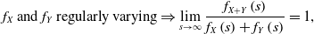 \begin{equation}f_X\text{ and }f_Y\text{ regularly varying}\Rightarrow\lim_{s\rightarrow \infty }\frac{f_{X+Y}\left( s\right) }{f_{X}\left(s\right) +f_{Y}\left( s\right) }=1,\end{equation}
where $f_{X+Y}(\!\cdot\!)$
is the convolution of
$f_{X+Y}(\!\cdot\!)$
is the convolution of $f_X(\!\cdot\!)$
and
$f_X(\!\cdot\!)$
and $f_Y(\!\cdot\!)$
. See, for example, Theorem 1.1 in Bingham et al. (Reference Bingham, Goldie and Omey2006) for a proof.
$f_Y(\!\cdot\!)$
. See, for example, Theorem 1.1 in Bingham et al. (Reference Bingham, Goldie and Omey2006) for a proof.
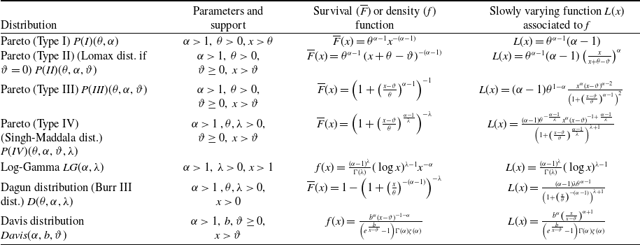
In Table 1, we summarize some distributions with regularly varying densities, along with the index and slowly varying function $L(\!\cdot\!)$
appearing in the representation of the density
$L(\!\cdot\!)$
appearing in the representation of the density $f(\!\cdot\!)$
as stated in Definition 2.1. The notation
$f(\!\cdot\!)$
as stated in Definition 2.1. The notation $\Gamma (\!\cdot\!)$
stands for the Gamma function and
$\Gamma (\!\cdot\!)$
stands for the Gamma function and $\zeta (\!\cdot\!)$
for the Riemann Zeta function. Note that the parameters of the distribution and density functions have been chosen to have index
$\zeta (\!\cdot\!)$
for the Riemann Zeta function. Note that the parameters of the distribution and density functions have been chosen to have index $\alpha$
in all cases. To this end, we may deviate from the standard parameter choices for these distributions. Type I and Type II Pareto, Log-Gamma, and Dagun distributions are often defined with a parameter
$\alpha$
in all cases. To this end, we may deviate from the standard parameter choices for these distributions. Type I and Type II Pareto, Log-Gamma, and Dagun distributions are often defined with a parameter $\beta=\alpha-1$
instead of the parameter
$\beta=\alpha-1$
instead of the parameter $\alpha$
which appears in Table 1. Type III and Type VI Pareto distributions are often specified with parameter
$\alpha$
which appears in Table 1. Type III and Type VI Pareto distributions are often specified with parameter $\gamma=\frac{\lambda}{\alpha-1}$
(
$\gamma=\frac{\lambda}{\alpha-1}$
( $\lambda=1$
in the case of Type III) instead of
$\lambda=1$
in the case of Type III) instead of $\alpha$
. Note that the support is
$\alpha$
. Note that the support is $(\vartheta,\infty)$
for certain distributions listed in Table 1. In the remainder of this paper, we assume that the supports of X and Y (and hence of their sum S) are
$(\vartheta,\infty)$
for certain distributions listed in Table 1. In the remainder of this paper, we assume that the supports of X and Y (and hence of their sum S) are $(0,\infty)$
. If the support of the variables is of the form
$(0,\infty)$
. If the support of the variables is of the form $(\vartheta,\infty)$
, we can either extend the density function
$(\vartheta,\infty)$
, we can either extend the density function $f\left(\cdot\right)$
by assuming
$f\left(\cdot\right)$
by assuming $f(x)=0$
for
$f(x)=0$
for $x\in \left(0,\vartheta\right]$
or shift the random variable under consideration by
$x\in \left(0,\vartheta\right]$
or shift the random variable under consideration by $\vartheta$
. Note that, even though assuming a regularly varying density is more restrictive than assuming regular variation of the survival function, it is not such a restrictive assumption in practice since, as seen in Table 1, it is verified by many well-known heavy-tailed distributions.
$\vartheta$
. Note that, even though assuming a regularly varying density is more restrictive than assuming regular variation of the survival function, it is not such a restrictive assumption in practice since, as seen in Table 1, it is verified by many well-known heavy-tailed distributions.
Families of distributions with regularly varying densities with index $\alpha$
.
$\alpha$
.
To conduct our study, we need to impose a condition known in the literature as asymptotic smoothness after Barbe and McCormick (Reference Barbe and McCormick2005) and recalled next.
Definition 2.2. A density function $f(\!\cdot\!)$
defined on
$f(\!\cdot\!)$
defined on $\left(0,\infty\right)$
is said to be asymptotically smooth with index
$\left(0,\infty\right)$
is said to be asymptotically smooth with index $\alpha \gt1$
if
$\alpha \gt1$
if
 \begin{equation*}\lim_{\delta \rightarrow 0}\limsup_{t\rightarrow \infty }\sup_{0\lt|x|\leq\delta }\left\vert \frac{f(t(1-x))-f(t)}{xf(t)}-\alpha \right\vert =0.\end{equation*}
Asymptotically smooth functions are related to regularly varying ones with the same index. When $f(\!\cdot\!)$
is asymptotically smooth and differentiable, then it is also regularly varying with the same index. Conversely, if
$f(\!\cdot\!)$
is asymptotically smooth and differentiable, then it is also regularly varying with the same index. Conversely, if $f(\!\cdot\!)$
is regularly varying, differentiable and has an ultimately monotone derivative, then it is asymptotically smooth (see Proposition 2.1 in Barbe and McCormick, Reference Barbe and McCormick2005). It must be remarked that all regularly varying densities considered in Table 1 have ultimately monotone derivatives and therefore are asymptotically smooth. The proof of this statement is given in Appendix A.
$f(\!\cdot\!)$
is regularly varying, differentiable and has an ultimately monotone derivative, then it is asymptotically smooth (see Proposition 2.1 in Barbe and McCormick, Reference Barbe and McCormick2005). It must be remarked that all regularly varying densities considered in Table 1 have ultimately monotone derivatives and therefore are asymptotically smooth. The proof of this statement is given in Appendix A.
2.2. Representation of the conditional expectation given the sum in terms of size biasing
Let us consider a nonnegative random variable X with distribution function $F_{X}$
and finite and strictly positive expected value. If X is a random variable having a regularly varying density with index
$F_{X}$
and finite and strictly positive expected value. If X is a random variable having a regularly varying density with index $\alpha \gt1$
, it is well known that
$\alpha \gt1$
, it is well known that $k\lt\alpha -1$
implies
$k\lt\alpha -1$
implies $\mathrm{E}[X^{k}]\lt\infty $
. Hence,
$\mathrm{E}[X^{k}]\lt\infty $
. Hence, $\mathrm{E}[X]\lt\infty$
if
$\mathrm{E}[X]\lt\infty$
if $\alpha\gt2$
, and we retain this assumption for all variables considered throughout this paper. The distribution function of the size-biased version
$\alpha\gt2$
, and we retain this assumption for all variables considered throughout this paper. The distribution function of the size-biased version $\widetilde{X}$
of X is then given by
$\widetilde{X}$
of X is then given by
 \begin{equation*}\mathrm{P}[\widetilde{X}\leq t]=\frac{1}{\mathrm{E}[X]}\int_{0}^{t}x \mathrm{d}F_{X}(x),\hspace{2mm}t\geq 0.\end{equation*}
We refer the reader to Arratia et al. (Reference Arratia, Goldstein and Kochman2019) for an introduction to the size-biased transform. Note that for any random variables X, Y with joint density f, the regression function can be expressed as
 \begin{align*}m_X(s)=\frac{1}{f_{X+Y}(s)}\int_0^s x f(x,s-x)\mathrm{d}x.\end{align*}
Under our framework, that is, considering independent random variables, in Denuit (Reference Denuit2019) a representation for the regression function $m_{X}(\!\cdot\!)$
is established in terms of the size-biased transform of X. Assume that X and Y have finite means and respective probability density functions
$m_{X}(\!\cdot\!)$
is established in terms of the size-biased transform of X. Assume that X and Y have finite means and respective probability density functions $f_X(\!\cdot\!)$
and
$f_X(\!\cdot\!)$
and $f_Y(\!\cdot\!)$
. Since X possesses a density function
$f_Y(\!\cdot\!)$
. Since X possesses a density function $f_{X}(\!\cdot\!)$
and its expected value is finite, its size-biased version
$f_{X}(\!\cdot\!)$
and its expected value is finite, its size-biased version $\widetilde{X}$
also possesses a density given by
$\widetilde{X}$
also possesses a density given by $f_{\widetilde{X}}(x)=xf_{X}(x)/\mathrm{E}[X]$
. If
$f_{\widetilde{X}}(x)=xf_{X}(x)/\mathrm{E}[X]$
. If $\widetilde{X}$
is independent of Y, then the representation
$\widetilde{X}$
is independent of Y, then the representation
 \begin{equation}m_{X}(s)=\mathrm{E}[X] \frac{f_{\widetilde{X}+Y}(s)}{f_{X+Y}(s)}\end{equation}
holds true for any $s\gt 0$
.
$s\gt 0$
.
2.3. Minimum limit value of ${\textbf{\textit{m}}}_{\textbf{\textit{X}}}( \!\cdot\! ) $

Understanding the asymptotic behavior of $m_{X}\left( s\right) $
as s gets large is important in practice. For example, in the case of risk sharing,
$m_{X}\left( s\right) $
as s gets large is important in practice. For example, in the case of risk sharing, $m_{X}\left( s\right) $
represents the contribution to be paid by the participant bringing X in the event of a large pool loss. If the supports of X and Y are not bounded, we might expect this contribution to tend toward infinity when s tends to infinity. We shall see that this is not always the case. However, under some technical assumptions, there exists a minimum value of the limit below which the contribution cannot fall, which is
$m_{X}\left( s\right) $
represents the contribution to be paid by the participant bringing X in the event of a large pool loss. If the supports of X and Y are not bounded, we might expect this contribution to tend toward infinity when s tends to infinity. We shall see that this is not always the case. However, under some technical assumptions, there exists a minimum value of the limit below which the contribution cannot fall, which is $\mathrm{E}[X]$
as established below. This limit is reached in particular when X and Y have regularly varying densities with tail indices whose difference is larger than 1 as it will become clear in the next section.
$\mathrm{E}[X]$
as established below. This limit is reached in particular when X and Y have regularly varying densities with tail indices whose difference is larger than 1 as it will become clear in the next section.
Proposition 2.3. Assume that X and Y have densities $f_{X}( \!\cdot\! ) $
and
$f_{X}( \!\cdot\! ) $
and $ f_{Y}( \!\cdot\! ) $
such that
$ f_{Y}( \!\cdot\! ) $
such that $f_{Y}( \!\cdot\! ) $
is bounded and ultimately decreasing, that is there exists
$f_{Y}( \!\cdot\! ) $
is bounded and ultimately decreasing, that is there exists $y_{0}$
such that
$y_{0}$
such that $ f_{Y}( \!\cdot\! ) $
is decreasing over
$ f_{Y}( \!\cdot\! ) $
is decreasing over $(y_{0},\infty )$
. Moreover, assume that
$(y_{0},\infty )$
. Moreover, assume that $\sup_{ x\in (s-y_{0},s)}f_{X}\left( x\right) =\mathrm{o} (f_{X+Y}(s))$
as
$\sup_{ x\in (s-y_{0},s)}f_{X}\left( x\right) =\mathrm{o} (f_{X+Y}(s))$
as $s\rightarrow \infty $
, then
$s\rightarrow \infty $
, then
 \begin{equation*} \liminf_{s\rightarrow \infty } m_{X}\left( s\right) \geq \mathrm{E}[X]. \end{equation*}
Proof. Note that, for $s\gt y_0$
,
$s\gt y_0$
,
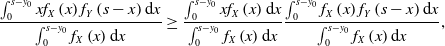
 \begin{equation} m_{X}\left( s\right) =\frac{\int_{0}^{s}xf_{X}\left( x\right) f_{Y}\left( s-x\right) \mathrm{d}x}{\int_{0}^{s}f_{X}\left( x\right) f_{Y}\left( s-x\right) \mathrm{d}x} \geq \frac{\int_{0}^{s-y_{0}}xf_{X}\left( x\right) f_{Y}\left( s-x\right) \mathrm{d}x }{\int_{0}^{s-y_{0}}f_{X}\left( x\right) f_{Y}\left( s-x\right) \mathrm{d}x+\int_{s-y_{0}}^{s}f_{X}\left( x\right) f_{Y}\left( s-x\right) \mathrm{d}x}. \end{equation}
Since $f_{Y}\left( s-\cdot \right) $
is increasing on
$f_{Y}\left( s-\cdot \right) $
is increasing on $\left( 0,s-y_{0}\right) $
, we have
$\left( 0,s-y_{0}\right) $
, we have
 \begin{equation*} \mathrm{E}[Xf_{Y}\left( s-X\right) |X\leq s-y_{0}]\geq \mathrm{E}[X|X\leq s-y_{0}]\mathrm{E}[f_{Y}\left( s-X\right) |X\leq s-y_{0}] \end{equation*}
or equivalently
 \begin{equation*} \frac{\int_{0}^{s-y_{0}}xf_{X}\left( x\right) f_{Y}\left( s-x\right) \mathrm{d}x}{ \int_{0}^{s-y_{0}}f_{X}\left( x\right) \mathrm{d}x}\geq \frac{ \int_{0}^{s-y_{0}}xf_{X}\left( x\right) \mathrm{d}x}{\int_{0}^{s-y_{0}}f_{X}\left( x\right) \mathrm{d}x}\frac{\int_{0}^{s-y_{0}}f_{X}\left( x\right) f_{Y}\left( s-x\right) \mathrm{d}x}{\int_{0}^{s-y_{0}}f_{X}\left( x\right) \mathrm{d}x}, \end{equation*}
what implies
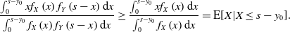 \begin{equation*} \frac{\int_{0}^{s-y_{0}}xf_{X}\left( x\right) f_{Y}\left( s-x\right) \mathrm{d}x}{\int_{0}^{s-y_{0}}f_{X}\left( x\right) f_{Y}\left( s-x\right) \mathrm{d}x}\geq \frac{ \int_{0}^{s-y_{0}}xf_{X}\left( x\right) \mathrm{d}x}{\int_{0}^{s-y_{0}}f_{X}\left( x\right) \mathrm{d}x}=\mathrm{E}[X|X\leq s-y_{0}]. \end{equation*}
Therefore, we deduce that
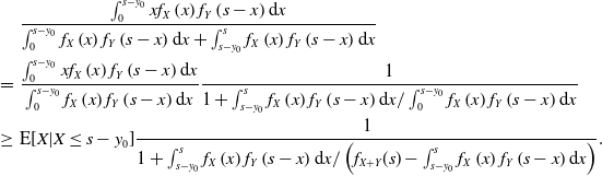 \begin{eqnarray} &&\frac{\int_{0}^{s-y_{0}}xf_{X}\left( x\right) f_{Y}\left( s-x\right) \mathrm{d}x}{ \int_{0}^{s-y_{0}}f_{X}\left( x\right) f_{Y}\left( s-x\right) \mathrm{d}x+\int_{s-y_{0}}^{s}f_{X}\left( x\right) f_{Y}\left( s-x\right) \mathrm{d}x} \\ &=&\frac{\int_{0}^{s-y_{0}}xf_{X}\left( x\right) f_{Y}\left( s-x\right) \mathrm{d}x}{ \int_{0}^{s-y_{0}}f_{X}\left( x\right) f_{Y}\left( s-x\right) \mathrm{d}x}\frac{1}{ 1+\int_{s-y_{0}}^{s}f_{X}\left( x\right) f_{Y}\left( s-x\right) \mathrm{d}x/\int_{0}^{s-y_{0}}f_{X}\left( x\right) f_{Y}\left( s-x\right) \mathrm{d}x} \nonumber\\ &\geq &\mathrm{E}[X|X\leq s-y_{0}]\frac{1}{1+\int_{s-y_{0}}^{s}f_{X}\left( x\right) f_{Y}\left( s-x\right) \mathrm{d}x/\left(f_{X+Y}(s)-\int_{s-y_{0}}^{s}f_{X}\left( x\right) f_{Y}\left( s-x\right) \mathrm{d}x\right)} \nonumber. \end{eqnarray}
Moreover,
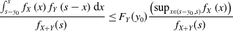 \begin{equation*}\frac{\int_{s-y_{0}}^{s}f_{X}\left( x\right)f_{Y}\left( s-x\right) \mathrm{d}x}{f_{X+Y}(s)}\leq F_Y(y_0)\frac{\left(\sup_{x\in (s-y_{0},s)}f_{X}\left( x\right) \right)}{f_{X+Y}(s)}\end{equation*}
and, since $\sup_{x\in (s-y_{0},s)}f_{X}\left( x\right) =\mathrm{o} (f_{X+Y}(s))$
as
$\sup_{x\in (s-y_{0},s)}f_{X}\left( x\right) =\mathrm{o} (f_{X+Y}(s))$
as $s\rightarrow \infty $
, it follows that
$s\rightarrow \infty $
, it follows that
 \begin{equation*}\lim_{s\rightarrow \infty }\frac{\int_{s-y_{0}}^{s}f_{X}\left( x\right)f_{Y}\left( s-x\right) \mathrm{d}x}{f_{X+Y}(s)}=0\end{equation*}
And, therefore
 \begin{equation*} \lim_{s\rightarrow \infty }\frac{1}{1+\int_{s-y_{0}}^{s}f_{X}\left( x\right) f_{Y}\left( s-x\right) \mathrm{d}x/ \left(f_{X+Y}(s)-\int_{s-y_{0}}^{s}f_{X}\left( x\right) f_{Y}\left( s-x\right) \mathrm{d}x\right)}=1 \end{equation*}
and, as $\lim_{s\rightarrow \infty }\mathrm{E}[X|X\leq s-y_{0}]=\mathrm{E}[X]$
, from (2.3) and (2.4),
$\lim_{s\rightarrow \infty }\mathrm{E}[X|X\leq s-y_{0}]=\mathrm{E}[X]$
, from (2.3) and (2.4), $\liminf_{s\rightarrow \infty } m_{X}\left( s\right) \geq \mathrm{E}[X]$
.
$\liminf_{s\rightarrow \infty } m_{X}\left( s\right) \geq \mathrm{E}[X]$
.
Remark 2.4. As a direct consequence of the Uniform convergence theorem for regularly varying functions (Theorem 1.5.2 in Bingham et al., Reference Bingham, Goldie and Teugels1987), if $f_X(\!\cdot\!)$
is a regularly varying density on
$f_X(\!\cdot\!)$
is a regularly varying density on $(0, \infty)$
, with tail index
$(0, \infty)$
, with tail index $\alpha _{X}$
, then
$\alpha _{X}$
, then $\sup_{s\in (x-y_{0},x)}f_{X}\left( s\right) =\mathrm{O}(f_{X}(x))$
. Considering
$\sup_{s\in (x-y_{0},x)}f_{X}\left( s\right) =\mathrm{O}(f_{X}(x))$
. Considering $f_Y(\!\cdot\!)$
as a second regularly varying density with respective index
$f_Y(\!\cdot\!)$
as a second regularly varying density with respective index $\alpha _{Y}$
such that
$\alpha _{Y}$
such that $\alpha_X\gt \alpha_Y$
, since
$\alpha_X\gt \alpha_Y$
, since $f_X(x)=\mathrm{o}(f_{Y}(x))$
, by Equation (2.1) the assumption
$f_X(x)=\mathrm{o}(f_{Y}(x))$
, by Equation (2.1) the assumption $\sup_{s\in (x-y_{0},x)}f_{X}\left( s\right) =\mathrm{o}(f_{X+Y}(x))$
as
$\sup_{s\in (x-y_{0},x)}f_{X}\left( s\right) =\mathrm{o}(f_{X+Y}(x))$
as $x\rightarrow \infty$
is verified.
$x\rightarrow \infty$
is verified.
2.4. Representation of the first derivative of the conditional expectation given the sum
Let us assume that the first derivative $f_Y'(\!\cdot\!)$
of the probability density function
$f_Y'(\!\cdot\!)$
of the probability density function $f_Y(\!\cdot\!)$
exists and is well defined. Let
$f_Y(\!\cdot\!)$
exists and is well defined. Let $(X_{1},Y_{1})$
and
$(X_{1},Y_{1})$
and $(X_{2},Y_{2})$
be independent copies of (X, Y), with respective sums
$(X_{2},Y_{2})$
be independent copies of (X, Y), with respective sums $S_{1}=X_{1}+Y_{1}$
and
$S_{1}=X_{1}+Y_{1}$
and $S_{2}=X_{2}+Y_{2}$
. Then Denuit and Robert (Reference Denuit and Robert2021a) demonstrated that the first derivative
$S_{2}=X_{2}+Y_{2}$
. Then Denuit and Robert (Reference Denuit and Robert2021a) demonstrated that the first derivative $m_X'(\!\cdot\!)$
of
$m_X'(\!\cdot\!)$
of $m_X(\!\cdot\!)$
exists and can be represented as
$m_X(\!\cdot\!)$
exists and can be represented as
 \begin{equation*}m_{X}^{\prime }(s)=\frac{1}{4}\mathrm{E}\left[ \left. \left(X_{1}-X_{2}\right) \left( \frac{f_{Y}^{\prime }(Y_{1})}{f_{Y}(Y_{1})}-\frac{f_{Y}^{\prime }(Y_{2})}{f_{Y}(Y_{2})}\right) \mathrm{I}\left[ X_{1} \gt X_{2}\right] \right\vert S_{1}=s,S_{2}=s\right]\end{equation*}
where $\mathrm{I}[\cdot]$
denotes the indicator function (equal to 1 when the condition appearing within brackets is fulfilled and to 0 otherwise). In the latter expression, the inequality
$\mathrm{I}[\cdot]$
denotes the indicator function (equal to 1 when the condition appearing within brackets is fulfilled and to 0 otherwise). In the latter expression, the inequality $Y_{1}\lt Y_{2}$
must hold true because
$Y_{1}\lt Y_{2}$
must hold true because $X_{1}\gt X_{2}$
and the sums
$X_{1}\gt X_{2}$
and the sums $X_{1}+Y_{1}$
and
$X_{1}+Y_{1}$
and $X_{2}+Y_{2}$
are constrained to be equal to some fixed value s. We deduce that if
$X_{2}+Y_{2}$
are constrained to be equal to some fixed value s. We deduce that if $f_{Y}(\!\cdot\!)$
is assumed to be log-concave, that is
$f_{Y}(\!\cdot\!)$
is assumed to be log-concave, that is $\log f_{Y}(\!\cdot\!)$
is concave, then the ratio
$\log f_{Y}(\!\cdot\!)$
is concave, then the ratio $f_{Y}^{\prime }(\!\cdot\!)/f_{Y}(\!\cdot\!)$
is decreasing and the second factor in the last conditional expectation must thus be positive. Therefore
$f_{Y}^{\prime }(\!\cdot\!)/f_{Y}(\!\cdot\!)$
is decreasing and the second factor in the last conditional expectation must thus be positive. Therefore $m_{X}^{\prime }(s)\geq 0$
for any
$m_{X}^{\prime }(s)\geq 0$
for any $s\gt 0$
. Log-concavity of
$s\gt 0$
. Log-concavity of $f_Y(\!\cdot\!)$
thus guarantees that
$f_Y(\!\cdot\!)$
thus guarantees that $m_X(\!\cdot\!)$
is non-decreasing.
$m_X(\!\cdot\!)$
is non-decreasing.
This expression clarifies the role that log-concavity plays in the monotonicity of $m_X(\!\cdot\!)$
. However, it must be remarked that, under the assumption of log-concavity, not only
$m_X(\!\cdot\!)$
. However, it must be remarked that, under the assumption of log-concavity, not only $m_X(\!\cdot\!)$
is non-decreasing, but the variable
$m_X(\!\cdot\!)$
is non-decreasing, but the variable $\lbrace X\mid S=s\rbrace$
is non-decreasing in s in the usual stochastic order. This means that the expected value of any increasing transformation of the variable is non-decreasing in the conditioning value s of S. This result is a consequence of Section 2 in Efron (Reference Efron1965), and a proof computing
$\lbrace X\mid S=s\rbrace$
is non-decreasing in s in the usual stochastic order. This means that the expected value of any increasing transformation of the variable is non-decreasing in the conditioning value s of S. This result is a consequence of Section 2 in Efron (Reference Efron1965), and a proof computing $m_{X}^{\prime }(s)$
is provided in Saumard and Wellner (Reference Saumard and Wellner2014) using symmetrization arguments for independent log-concave variables.
$m_{X}^{\prime }(s)$
is provided in Saumard and Wellner (Reference Saumard and Wellner2014) using symmetrization arguments for independent log-concave variables.
Consider a regularly varying density $f(\!\cdot\!)$
with tail index
$f(\!\cdot\!)$
with tail index $\alpha$
such that
$\alpha$
such that $f^{\prime }(\!\cdot\!)$
is ultimately monotonic (from Property A.1, this is the case for all distributions listed in Table 1). Then, we can derive from Karamata’s theorem (Karamata, Reference Karamata1933) that
$f^{\prime }(\!\cdot\!)$
is ultimately monotonic (from Property A.1, this is the case for all distributions listed in Table 1). Then, we can derive from Karamata’s theorem (Karamata, Reference Karamata1933) that
 \begin{equation*}\frac{f^{\prime }(x)}{f(x)}\sim -\alpha \frac{1}{x}\end{equation*}
and therefore $f^{\prime }(\!\cdot\!)/f(\!\cdot\!)$
cannot be ultimately decreasing. Hence, it is natural to investigate whether
$f^{\prime }(\!\cdot\!)/f(\!\cdot\!)$
cannot be ultimately decreasing. Hence, it is natural to investigate whether $m_{X}(\!\cdot\!)$
can be decreasing for some tail indices of X and Y and for some values s of S. This is precisely one of the questions investigated in the present paper. Therefore, the following sections will delve into, for X, Y independent, nonnegative random variables with well-defined density functions, how a heavier-tail of Y affects the monotonicity of
$m_{X}(\!\cdot\!)$
can be decreasing for some tail indices of X and Y and for some values s of S. This is precisely one of the questions investigated in the present paper. Therefore, the following sections will delve into, for X, Y independent, nonnegative random variables with well-defined density functions, how a heavier-tail of Y affects the monotonicity of $m_{X}(\!\cdot\!)$
.
$m_{X}(\!\cdot\!)$
.
3. Asymptotic level of the conditional expectation given the sum
When X and Y possess regularly varying density functions with respective indices $\alpha _{X}$
and
$\alpha _{X}$
and $\alpha _{Y}$
, it turns out that the asymptotic level of
$\alpha _{Y}$
, it turns out that the asymptotic level of $m_X(\!\cdot\!)$
depends on the difference in the tail indices
$m_X(\!\cdot\!)$
depends on the difference in the tail indices $\alpha_X$
and
$\alpha_X$
and $\alpha_Y$
. It is assumed that
$\alpha_Y$
. It is assumed that $\min\lbrace\alpha_{X},\alpha_{Y}\rbrace\gt2$
so that
$\min\lbrace\alpha_{X},\alpha_{Y}\rbrace\gt2$
so that $\mathrm{E}[X]\lt\infty$
and
$\mathrm{E}[X]\lt\infty$
and $\mathrm{E}[Y]\lt\infty$
. Throughout this section, we will also assume
$\mathrm{E}[Y]\lt\infty$
. Throughout this section, we will also assume $\alpha_X\geq \alpha_Y$
. If
$\alpha_X\geq \alpha_Y$
. If $\alpha_X\lt\alpha_Y$
, it will be sufficient to interchange the indices
$\alpha_X\lt\alpha_Y$
, it will be sufficient to interchange the indices $\alpha_X$
and
$\alpha_X$
and $\alpha_Y$
in the results. Note that, under the assumption
$\alpha_Y$
in the results. Note that, under the assumption $\alpha_X\geq \alpha_Y$
, the next result shows that
$\alpha_X\geq \alpha_Y$
, the next result shows that $m_Y\left(\cdot\right)$
diverges, no matter the size of the difference between the indices:
$m_Y\left(\cdot\right)$
diverges, no matter the size of the difference between the indices:
Proposition 3.1. If X and Y possess regularly varying densities $f_X(\!\cdot\!)$
and
$f_X(\!\cdot\!)$
and $f_Y(\!\cdot\!)$
with respective indices
$f_Y(\!\cdot\!)$
with respective indices $\alpha _{X}$
and
$\alpha _{X}$
and $\alpha _{Y}$
such that
$\alpha _{Y}$
such that $\alpha_Y\leq\alpha_X$
, then
$\alpha_Y\leq\alpha_X$
, then $m_Y\left(s\right)\rightarrow \infty$
as
$m_Y\left(s\right)\rightarrow \infty$
as $s \rightarrow \infty$
.
$s \rightarrow \infty$
.
Proof. From (2.2), $m_{Y}(s)=\mathrm{E}[Y] \frac{f_{\widetilde{Y}+X}(s)}{f_{Y+X}(s)}$
, where
$m_{Y}(s)=\mathrm{E}[Y] \frac{f_{\widetilde{Y}+X}(s)}{f_{Y+X}(s)}$
, where $\widetilde{Y}$
is the size-biased transformation of Y. Note that, since
$\widetilde{Y}$
is the size-biased transformation of Y. Note that, since $f_Y(\!\cdot\!)$
is regularly varying with index
$f_Y(\!\cdot\!)$
is regularly varying with index $\alpha_Y\gt2$
,
$\alpha_Y\gt2$
, $f_{\widetilde{Y}}(\!\cdot\!)$
is regularly varying with index
$f_{\widetilde{Y}}(\!\cdot\!)$
is regularly varying with index $1\lt\alpha_{\widetilde{Y}}=\alpha_Y-1\lt\alpha_{Y}$
. Therefore,
$1\lt\alpha_{\widetilde{Y}}=\alpha_Y-1\lt\alpha_{Y}$
. Therefore, $f_Y(s)=o\left(f_{\widetilde{Y}}(s)\right)$
. As
$f_Y(s)=o\left(f_{\widetilde{Y}}(s)\right)$
. As $f_X(\!\cdot\!)$
is a regularly varying density with index
$f_X(\!\cdot\!)$
is a regularly varying density with index $\alpha_X\geq \alpha_Y$
, it holds that
$\alpha_X\geq \alpha_Y$
, it holds that $f_X(s)=o\left(f_{\widetilde{Y}}(s)\right)$
and:
$f_X(s)=o\left(f_{\widetilde{Y}}(s)\right)$
and:
 \begin{equation} m_{Y}(s)\sim \mathrm{E}[Y] \frac{f_{\widetilde{Y}}(s)+f_X(s)}{f_{Y}(s)+f_{X}(s)}=\mathrm{E}[Y] \frac{f_{\widetilde{Y}}(s)+o\left(f_{\widetilde{Y}}(s)\right)}{o\left(f_{\widetilde{Y}}(s)\right)+o\left(f_{\widetilde{Y}}(s)\right)}. \end{equation}
Hence, from this expression we conclude that $m_Y\left(s\right)\rightarrow \infty$
as
$m_Y\left(s\right)\rightarrow \infty$
as $s \rightarrow \infty$
.
$s \rightarrow \infty$
.
From Proposition 5.1 in Denuit and Robert (Reference Denuit and Robert2020) and since variables with regularly varying densities have regularly varying tails, if $\alpha_X\gt\alpha_Y$
, then, as s tends to infinity,
$\alpha_X\gt\alpha_Y$
, then, as s tends to infinity, $m_X(s)=o(s)$
. Although no information can be obtained with respect to the asymptotic level or the monotonicity of
$m_X(s)=o(s)$
. Although no information can be obtained with respect to the asymptotic level or the monotonicity of $m_X(\!\cdot\!)$
. Therefore, in order to study the behavior of
$m_X(\!\cdot\!)$
. Therefore, in order to study the behavior of $m_X\left(\cdot\right)$
, the following three cases can be distinguished.
$m_X\left(\cdot\right)$
, the following three cases can be distinguished.
3.1. Difference in tail indices larger than 1 (
$\alpha_X-\alpha_Y\gt1$
)

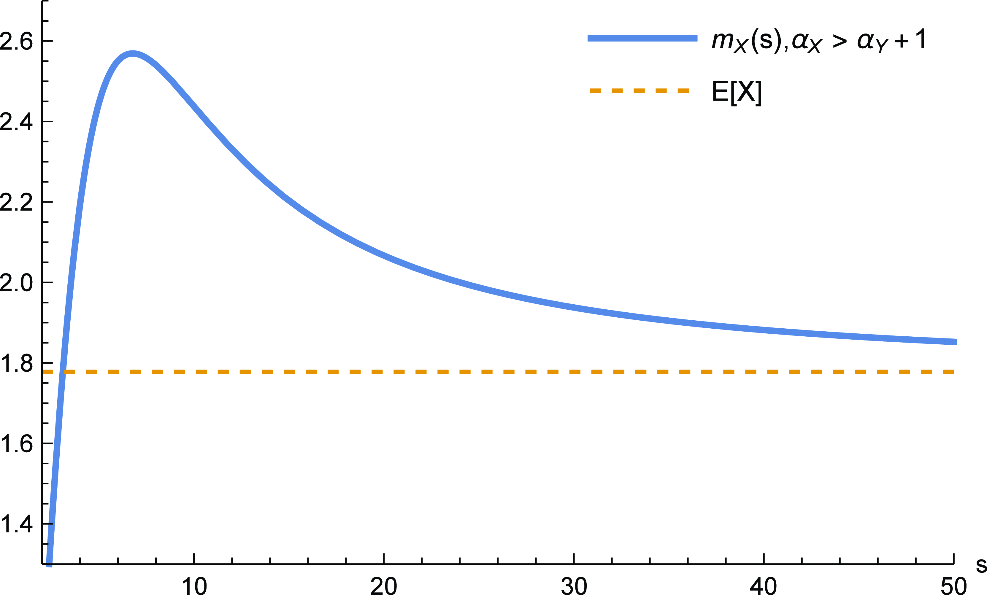
The next result shows that when the difference between tail indices exceeds 1, the conditional expectation given the sum tends to the expected value for the term with a larger index, as the sum tends to infinity.
Proposition 3.2. If X and Y possess regularly varying densities $f_X(\!\cdot\!)$
and
$f_X(\!\cdot\!)$
and $f_Y(\!\cdot\!)$
with respective indices
$f_Y(\!\cdot\!)$
with respective indices $\alpha _{X}$
and
$\alpha _{X}$
and $\alpha _{Y}$
such that
$\alpha _{Y}$
such that $\alpha_{X}\gt\alpha _{Y}+1$
, then
$\alpha_{X}\gt\alpha _{Y}+1$
, then
 \begin{equation*}\lim_{s\rightarrow \infty }m_{X}(s)=\mathrm{E}\left[ X\right].\end{equation*}
Proof. Since $f_{X}(\!\cdot\!)$
is regularly varying with index
$f_{X}(\!\cdot\!)$
is regularly varying with index $\alpha _{X}\gt2$
, we have that
$\alpha _{X}\gt2$
, we have that $f_{\widetilde{X}}(\!\cdot\!)$
is regularly varying with index
$f_{\widetilde{X}}(\!\cdot\!)$
is regularly varying with index $\alpha _{\widetilde{X}}=\alpha _{X}-1$
. As
$\alpha _{\widetilde{X}}=\alpha _{X}-1$
. As $\alpha _{X}\gt\alpha _{Y}+1$
, then
$\alpha _{X}\gt\alpha _{Y}+1$
, then $\alpha _{\widetilde{X}}\gt\alpha _{Y}$
and, therefore,
$\alpha _{\widetilde{X}}\gt\alpha _{Y}$
and, therefore, $f_{\widetilde{X}}\left( s\right) =o\left(f_{Y}\left( s\right) \right) $
and
$f_{\widetilde{X}}\left( s\right) =o\left(f_{Y}\left( s\right) \right) $
and $f_{X}\left( s\right) =o\left( f_{Y}\left( s\right) \right) $
, As a consequence of (2.1), then
$f_{X}\left( s\right) =o\left( f_{Y}\left( s\right) \right) $
, As a consequence of (2.1), then
 \begin{equation*}\lim_{s\rightarrow \infty }m_{X}(s)=\mathrm{E}\left[ X\right]\lim_{s\rightarrow \infty }\frac{f_{\widetilde{X}}\left( s\right) +f_{Y}\left(s\right) }{f_{X}\left( s\right) +f_{Y}\left( s\right) } = \mathrm{E}[X].\end{equation*}
This ends the proof.
Note that a direct implication of Proposition 3.2 for absolutely continuous distributions is that $m_X(\!\cdot\!)$
is bounded. The following result shows that
$m_X(\!\cdot\!)$
is bounded. The following result shows that $m_X(\!\cdot\!)$
cannot be monotonic over
$m_X(\!\cdot\!)$
cannot be monotonic over $(0,\infty)$
in the case considered in Proposition 3.2.
$(0,\infty)$
in the case considered in Proposition 3.2.
Proposition 3.3. Assume that X and Y are as described in Proposition 3.2, then there exists a nonempty interval in $(0,\infty)$
where
$(0,\infty)$
where $m_{X}(\!\cdot\!)$
is decreasing.
$m_{X}(\!\cdot\!)$
is decreasing.
Proof. Let us proceed by contradiction. Assume that $m_{X}(\!\cdot\!)$
is increasing on
$m_{X}(\!\cdot\!)$
is increasing on $(0,\infty)$
. Notice that
$(0,\infty)$
. Notice that $m_{X}(\!\cdot\!)$
is a positive and continuous function such that
$m_{X}(\!\cdot\!)$
is a positive and continuous function such that $m_{X}(0)=0$
and
$m_{X}(0)=0$
and $\lim_{s\rightarrow \infty }m_{X}(s)=\mathrm{E}\left[ X\right] $
by Proposition 3.2. Moreover,
$\lim_{s\rightarrow \infty }m_{X}(s)=\mathrm{E}\left[ X\right] $
by Proposition 3.2. Moreover, $\mathrm{E}[X]=\mathrm{E}[m_{X}(S)]$
. If
$\mathrm{E}[X]=\mathrm{E}[m_{X}(S)]$
. If $m_{X}(\!\cdot\!)$
is increasing on
$m_{X}(\!\cdot\!)$
is increasing on $\left( 0,\infty \right) $
and, since both variables are continuous, we do, however, deduce that
$\left( 0,\infty \right) $
and, since both variables are continuous, we do, however, deduce that $\mathrm{E}[m_{X}(S)] \lt \mathrm{E}\left[ X\right] $
, which is a contradiction. This ends the proof.
$\mathrm{E}[m_{X}(S)] \lt \mathrm{E}\left[ X\right] $
, which is a contradiction. This ends the proof.
The following example illustrates the behavior of $m_X(\!\cdot\!)$
in the case where the difference in the tail indices exceeds 1.
$m_X(\!\cdot\!)$
in the case where the difference in the tail indices exceeds 1.
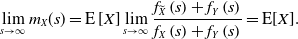
Example 3.4. Let us consider two independent random variables $X\sim LG(\alpha_{X},\lambda_X)$
and
$X\sim LG(\alpha_{X},\lambda_X)$
and $Y\sim P(IV)(\theta,\alpha_{Y},\vartheta,\lambda_Y)$
such that
$Y\sim P(IV)(\theta,\alpha_{Y},\vartheta,\lambda_Y)$
such that $\alpha_{X}\gt\alpha_Y+1$
. Figure 1 shows a numerical representation considering the parameter values
$\alpha_{X}\gt\alpha_Y+1$
. Figure 1 shows a numerical representation considering the parameter values $\vartheta =\theta =1$
,
$\vartheta =\theta =1$
, $\lambda_X=\lambda_Y=2$
,
$\lambda_X=\lambda_Y=2$
, $\alpha_{X}=5$
, and
$\alpha_{X}=5$
, and $\alpha_Y=2$
. We can observe that
$\alpha_Y=2$
. We can observe that $m_{X}(\!\cdot\!)$
is not monotonic over
$m_{X}(\!\cdot\!)$
is not monotonic over $(0,\infty)$
, in accordance with Proposition 3.3. Here,
$(0,\infty)$
, in accordance with Proposition 3.3. Here, $m_{X}(\!\cdot\!)$
reaches its maximum and starts decreasing beyond
$m_{X}(\!\cdot\!)$
reaches its maximum and starts decreasing beyond $F_S^{-1}(0.91)$
.
$F_S^{-1}(0.91)$
.
Conditional expectation $m_X(\!\cdot\!)$
(solid line) and horizontal line at
$m_X(\!\cdot\!)$
(solid line) and horizontal line at $\mathrm{E}[X]$
(dashed line) when
$\mathrm{E}[X]$
(dashed line) when $X\sim LG(\alpha_{X},\lambda_X)$
and
$X\sim LG(\alpha_{X},\lambda_X)$
and $Y\sim P(IV)(\theta,\alpha_{Y},\vartheta,\lambda_Y)$
with
$Y\sim P(IV)(\theta,\alpha_{Y},\vartheta,\lambda_Y)$
with $\vartheta =\theta =1$
,
$\vartheta =\theta =1$
, $\lambda_X=\lambda_Y=2$
,
$\lambda_X=\lambda_Y=2$
, $\alpha_{X}=5$
, and
$\alpha_{X}=5$
, and $\alpha_Y=2$
.
$\alpha_Y=2$
.
Let us remark that the preceding results serve to enhance the discussion provided in Section 4 of Major and Mildenhall (Reference Major and Mildenhall2020) and Section 14.3 of Mildenhall and Major (Reference Mildenhall and Major2022), in which several examples where, for combinations of heavy-tailed units, $m_X(\!\cdot\!)$
may not be monotone. The authors also discussed that a light-tailed unit combined with a heavy-tailed unit could lead to analogous behaviors, and this is, indeed, the case. Note that Propositions 3.2 and 3.3 can be extended to scenarios where X does not have a regularly varying density but has a density dominated by
$m_X(\!\cdot\!)$
may not be monotone. The authors also discussed that a light-tailed unit combined with a heavy-tailed unit could lead to analogous behaviors, and this is, indeed, the case. Note that Propositions 3.2 and 3.3 can be extended to scenarios where X does not have a regularly varying density but has a density dominated by $f_Y(\!\cdot\!)$
in the tail. This follows from Theorem 2.1 in Bingham et al. (Reference Bingham, Goldie and Omey2006), which states that, if
$f_Y(\!\cdot\!)$
in the tail. This follows from Theorem 2.1 in Bingham et al. (Reference Bingham, Goldie and Omey2006), which states that, if $f_X(\!\cdot\!)$
and
$f_X(\!\cdot\!)$
and $f_Y(\!\cdot\!)$
are probability densities on
$f_Y(\!\cdot\!)$
are probability densities on $\mathbb{R}$
, with
$\mathbb{R}$
, with $f_Y(\!\cdot\!)$
regularly varying and
$f_Y(\!\cdot\!)$
regularly varying and $f_X(x)=o(f_Y(x))$
as x tends to infinity, then
$f_X(x)=o(f_Y(x))$
as x tends to infinity, then $\lim_{s\rightarrow \infty}\frac{f_{X+Y}(s)}{f_Y(s)}=1$
.
$\lim_{s\rightarrow \infty}\frac{f_{X+Y}(s)}{f_Y(s)}=1$
.
Corollary 3.5. If X and Y possess densities $f_X(\!\cdot\!)$
and
$f_X(\!\cdot\!)$
and $f_Y(\!\cdot\!)$
with
$f_Y(\!\cdot\!)$
with $f_Y(\!\cdot\!)$
regularly varying and
$f_Y(\!\cdot\!)$
regularly varying and $f_X(x)=o(\frac{f_Y(x)}{x})$
as x tends to infinity, then
$f_X(x)=o(\frac{f_Y(x)}{x})$
as x tends to infinity, then $\lim_{s\rightarrow \infty }m_{X}(s)=\mathrm{E}\left[ X\right]$
and there exists a non-empty interval in
$\lim_{s\rightarrow \infty }m_{X}(s)=\mathrm{E}\left[ X\right]$
and there exists a non-empty interval in $(0,\infty)$
where
$(0,\infty)$
where $m_{X}(\!\cdot\!)$
is decreasing.
$m_{X}(\!\cdot\!)$
is decreasing.
Since $m_{X}(s)+m_{Y}(s)=s$
, both functions cannot decrease simultaneously. Therefore, if either
$m_{X}(s)+m_{Y}(s)=s$
, both functions cannot decrease simultaneously. Therefore, if either $m_{X}(\!\cdot\!)$
and
$m_{X}(\!\cdot\!)$
and $m_{Y}(\!\cdot\!)$
have a decreasing interval, as the other increases in such interval, it implies that, locally,
$m_{Y}(\!\cdot\!)$
have a decreasing interval, as the other increases in such interval, it implies that, locally, $m_{X}(S)$
and
$m_{X}(S)$
and $m_{Y}(S)$
are negatively dependent. This means that, given that S belongs to such interval,
$m_{Y}(S)$
are negatively dependent. This means that, given that S belongs to such interval, $m_{X}(S)$
tends to take larger values as
$m_{X}(S)$
tends to take larger values as $m_{Y}(S)$
takes smaller values and vice-versa. Although in the scenario considered in this section, even if the conditional expectation given the sum must decrease over some values of the sum according to Proposition 3.3, it is interesting to point out that, globally,
$m_{Y}(S)$
takes smaller values and vice-versa. Although in the scenario considered in this section, even if the conditional expectation given the sum must decrease over some values of the sum according to Proposition 3.3, it is interesting to point out that, globally, $m_{X}(S)$
and
$m_{X}(S)$
and $m_{Y}(S)$
always remain positively correlated. This is precisely stated next.
$m_{Y}(S)$
always remain positively correlated. This is precisely stated next.
While this paper considers random variables X and Y possessing regularly varying density functions, the next result holds more generally for any positive variables with finite second-order moments. Let us remark that, if X and Y possess regularly varying densities with tail indices $\alpha _{X}$
and
$\alpha _{X}$
and $\alpha _{Y}$
, respectively, then the assumption of finite second-order moments is equivalent to
$\alpha _{Y}$
, respectively, then the assumption of finite second-order moments is equivalent to $\min\{\alpha _{X},\alpha _{Y}\}\gt3$
.
$\min\{\alpha _{X},\alpha _{Y}\}\gt3$
.
Proposition 3.6. Considering random variables X and Y, if their second-order moments are finite, then
 \begin{equation} \mathrm{Cov}[m_{X}(S),m_{Y}(S)]\geq 0. \end{equation}
Proof. First notice that for any s in the support of $S=X+Y$
, we have
$S=X+Y$
, we have
 \begin{equation*}\mathrm{Var}\left[ X|S=s\right] =\mathrm{Var}\left[ X-s|S=s\right] =\mathrm{\ Var}\left[ -Y|S=s\right] =\mathrm{Var}\left[ Y|S=s\right] .\end{equation*}
This implies that
 \begin{equation} \mathrm{Var}[Y\mid S=s]=\mathrm{Var}[X\mid S=s].\end{equation}
Now, we can write
 \begin{equation*}0=\mathrm{Var}[S|S=s]=\mathrm{Var}[X|S=s]+\mathrm{Var}[Y\mid S=s]+2\mathrm{Cov}[X, Y|S=s].\end{equation*}
It follows from (3.3) that
 \begin{equation} \mathrm{Cov}[X, Y|S=s]=-\mathrm{Var}[X|S=s].\end{equation}
Then,
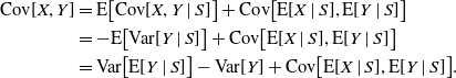 \begin{equation*}\begin{split}\mathrm{Cov}[X, Y]&= \mathrm{E}\big[\mathrm{Cov}[X, Y \mid S]\big]+\mathrm{Cov}\big[\mathrm{E}[X \mid S], \mathrm{E}[Y \mid S]\big] \\&= -\mathrm{E}\big[\mathrm{Var}[Y \mid S]\big]+\mathrm{Cov}\big[\mathrm{E}[X\mid S], \mathrm{E}[Y \mid S]\big] \\&= \mathrm{Var}\big[\mathrm{E}[Y \mid S]\big]-\mathrm{Var}[Y]+\mathrm{Cov}\big[\mathrm{E}[X \mid S], \mathrm{E}[Y \mid S]\big].\end{split}\end{equation*}
so that we get
 \begin{equation} \mathrm{Cov}\big[\mathrm{E}[X \mid S], \mathrm{E}[Y \mid S]\big]=\mathrm{Cov}[X, Y]+\mathrm{Var}[Y]-\mathrm{Var}\big[\mathrm{E}[Y \mid S]\big].\end{equation}
Considering (3.5), Jensen’s inequality ensures that $\mathrm{Var}[Y]\geq\mathrm{Var}\big[\mathrm{E}[Y \mid S]\big]$
. The announced inequality (3.2) finally follows from
$\mathrm{Var}[Y]\geq\mathrm{Var}\big[\mathrm{E}[Y \mid S]\big]$
. The announced inequality (3.2) finally follows from $\mathrm{Cov}[X, Y]=0$
.
$\mathrm{Cov}[X, Y]=0$
.
We can now briefly comment on the result stated in Proposition 3.5:
-
• As a direct consequence of (3.3),
$\mathrm{Var}[X\mid S]=\mathrm{Var}[Y\mid S]$
a.s. -
• We see from (3.4) that
$\mathrm{Cov}[X, Y|S=s]\leq 0$
for all s, which could be expected since both variables are positive and the sum is fixed. Therefore, a greater value taken by one of the variables is negatively influencing the second variable. Again, (3.4) implies
$\mathrm{Cov}[X, Y|S]=-\mathrm{Var}[X\mid S]$
a.s. Note that, considering variables with log-concave densities, X and Y would not only have a negative covariance given S but would also be negatively associated (see Theorem 2.8 in Joag-Dev and Proschan, Reference Joag-Dev and Proschan1983).


Regarding risk-sharing, positive dependence means that, overall, participants have common interests as their contributions are likely to be large or small together. This positive global relationship between $m_{X}(S)$
and
$m_{X}(S)$
and $m_{Y}(S)$
holds true even if the functions
$m_{Y}(S)$
holds true even if the functions $m_{X}(\!\cdot\!)$
and
$m_{X}(\!\cdot\!)$
and $m_{Y}(\!\cdot\!)$
are not everywhere increasing. When
$m_{Y}(\!\cdot\!)$
are not everywhere increasing. When $m_{X}(\!\cdot\!)$
and
$m_{X}(\!\cdot\!)$
and $m_{Y}(\!\cdot\!)$
refer to the contributions to the pool, if one of them decreases in terms of the total loss, it will then be at the expense of the other contribution assuming a greater part of such total loss. Inequality (3.2) indicates that if there are values for which the monotonicity of
$m_{Y}(\!\cdot\!)$
refer to the contributions to the pool, if one of them decreases in terms of the total loss, it will then be at the expense of the other contribution assuming a greater part of such total loss. Inequality (3.2) indicates that if there are values for which the monotonicity of $m_{X}(\!\cdot\!)$
and
$m_{X}(\!\cdot\!)$
and $m_{Y}(\!\cdot\!)$
differ, those must be values with a small probability of occurrence or with slight differences in the increasing/decreasing rate, as overall, the dependence remains positive.
$m_{Y}(\!\cdot\!)$
differ, those must be values with a small probability of occurrence or with slight differences in the increasing/decreasing rate, as overall, the dependence remains positive.
3.2. Difference in tail indices less than 1 (
$0\leq\alpha_X-\alpha_Y \lt 1$
)

When the difference between tail indices is less than 1, the conditional expectation given the sum is not bounded as the sum tends to infinity. This is in contrast with the preceding case.
Proposition 3.7. If X and Y possess regularly varying densities $f_X(\!\cdot\!)$
and
$f_X(\!\cdot\!)$
and $f_Y(\!\cdot\!)$
with respective indices
$f_Y(\!\cdot\!)$
with respective indices $\alpha _{X}$
and
$\alpha _{X}$
and $\alpha _{Y}$
such that
$\alpha _{Y}$
such that $\alpha_X\gt2$
and
$\alpha_X\gt2$
and $\alpha_Y\leq\alpha_X\lt\alpha_Y+1$
, then
$\alpha_Y\leq\alpha_X\lt\alpha_Y+1$
, then $m_X(s)\rightarrow \infty$
as
$m_X(s)\rightarrow \infty$
as $s\rightarrow \infty$
.
$s\rightarrow \infty$
.
Proof. Since $f_X(\!\cdot\!)$
is regularly varying with index
$f_X(\!\cdot\!)$
is regularly varying with index $\alpha_X\gt2$
,
$\alpha_X\gt2$
, $f_{\widetilde{X}}(\!\cdot\!)$
is regularly varying with index
$f_{\widetilde{X}}(\!\cdot\!)$
is regularly varying with index $\alpha_{\widetilde{X}}=\alpha_X-1\lt\alpha_Y$
. Because
$\alpha_{\widetilde{X}}=\alpha_X-1\lt\alpha_Y$
. Because $f_Y(\!\cdot\!)$
is a regularly varying density, it implies that
$f_Y(\!\cdot\!)$
is a regularly varying density, it implies that $f_Y(s)=o\left(f_{\widetilde{X}}(s)\right)$
. Since
$f_Y(s)=o\left(f_{\widetilde{X}}(s)\right)$
. Since $\alpha_{\widetilde{X}}\lt\alpha_X$
, it also follows that
$\alpha_{\widetilde{X}}\lt\alpha_X$
, it also follows that $f_X(s)=o\left(f_{\widetilde{X}}(s)\right)$
. Therefore, by (2.1):
$f_X(s)=o\left(f_{\widetilde{X}}(s)\right)$
. Therefore, by (2.1):
 \begin{align*}m_X(s)=\mathrm{E}[X] \frac{f_{\widetilde{X}+Y}(s)}{f_{X+Y}(s)}\sim \mathrm{E}[X] \frac{f_{\widetilde{X}}(s)+f_Y(s)}{f_X(s)+f_Y(s)}=\mathrm{E}[X] \frac{f_{\widetilde{X}}(s)+o\left(f_{\widetilde{X}}(s)\right)}{o\left(f_{\widetilde{X}}(s)\right)+o\left(f_{\widetilde{X}}(s)\right)}.\end{align*}
From this expression, we can see that, as $s\rightarrow \infty$
,
$s\rightarrow \infty$
, $m_X(s)\rightarrow \infty$
and the assertion follows.
$m_X(s)\rightarrow \infty$
and the assertion follows.
From the previous result, we know that $m_X\left(\cdot\right)$
diverges as
$m_X\left(\cdot\right)$
diverges as $s\rightarrow \infty$
. However, this is not sufficient to ensure that it is an increasing function. A variety of different behaviors may occur when the difference in tail indices is less than 1. Example 3.8 shows an increasing behavior of
$s\rightarrow \infty$
. However, this is not sufficient to ensure that it is an increasing function. A variety of different behaviors may occur when the difference in tail indices is less than 1. Example 3.8 shows an increasing behavior of $m_X(\!\cdot\!),$
while Example 3.9 shows that it may be decreasing over a range of central values. Note that we cannot ensure the monotonicity of
$m_X(\!\cdot\!),$
while Example 3.9 shows that it may be decreasing over a range of central values. Note that we cannot ensure the monotonicity of $m_X(\!\cdot\!)$
, but we can check it numerically over an interval (0,b) for a large b (e.g.
$m_X(\!\cdot\!)$
, but we can check it numerically over an interval (0,b) for a large b (e.g. $b\gt \mathrm{E}[X+Y]+ 10^2\mathrm{Var}[X+Y]$
). Finally, in Section 4, we will see under which cases it is asymptotically monotonic.
$b\gt \mathrm{E}[X+Y]+ 10^2\mathrm{Var}[X+Y]$
). Finally, in Section 4, we will see under which cases it is asymptotically monotonic.
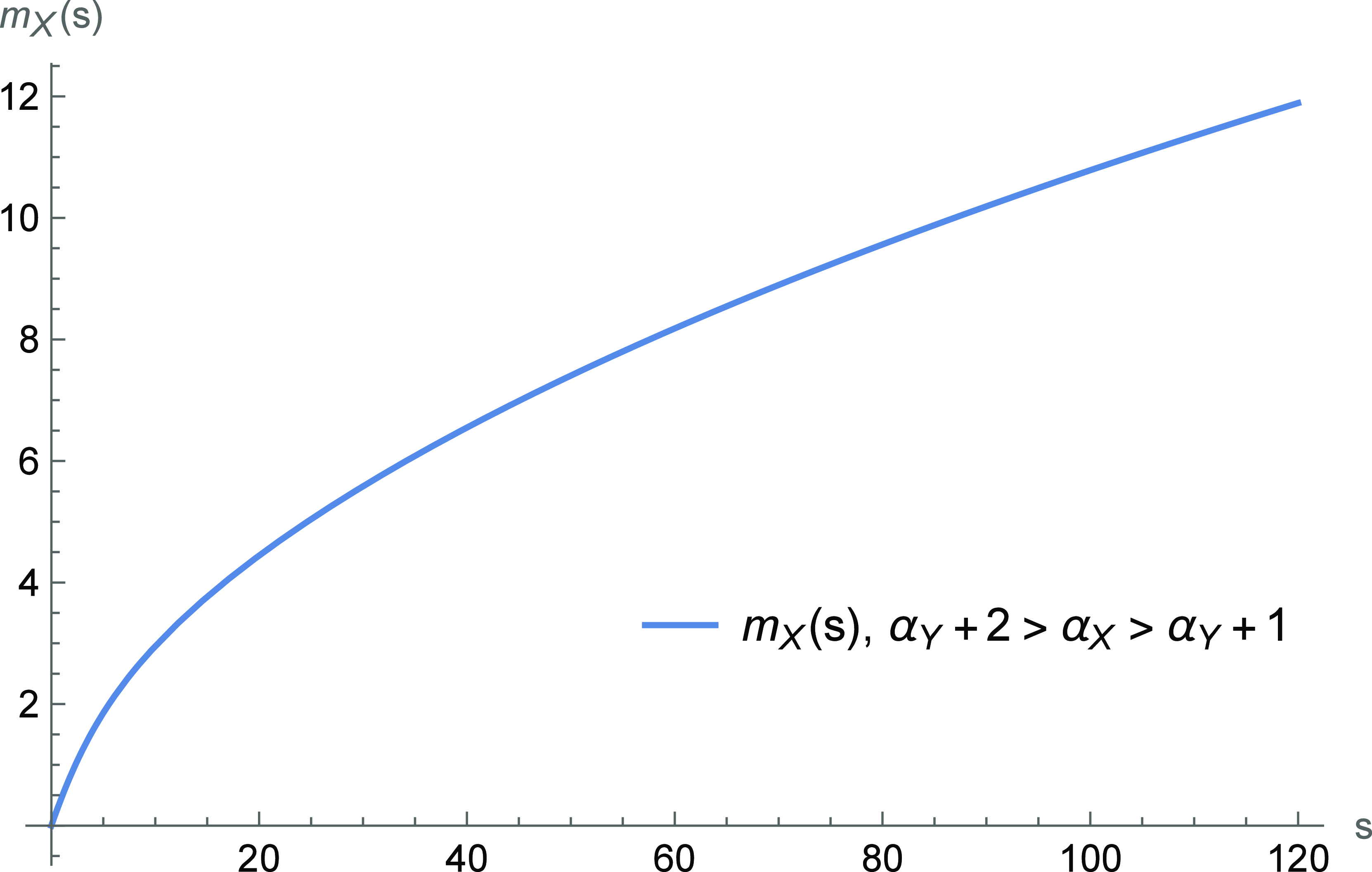
Example 3.8. Let us consider two independent random variables $X\sim P(II)(\theta, \alpha_{X},\vartheta)$
and
$X\sim P(II)(\theta, \alpha_{X},\vartheta)$
and $Y\sim P(II)(\theta, \alpha _{Y},\vartheta)$
such that
$Y\sim P(II)(\theta, \alpha _{Y},\vartheta)$
such that $\alpha _{X}=4.5$
,
$\alpha _{X}=4.5$
, $\alpha_Y=4$
,
$\alpha_Y=4$
, $\theta=1$
, and
$\theta=1$
, and $\vartheta=0$
. Figure 2 shows that
$\vartheta=0$
. Figure 2 shows that $m_X(\!\cdot\!)$
increases over (0, 120).
$m_X(\!\cdot\!)$
increases over (0, 120).
Conditional expectation $m_X(\!\cdot\!)$
when
$m_X(\!\cdot\!)$
when $X\sim P(II)(\theta, \alpha_{X},\vartheta)$
and
$X\sim P(II)(\theta, \alpha_{X},\vartheta)$
and $Y\sim P(II)(\theta, \alpha _{Y},\vartheta)$
with
$Y\sim P(II)(\theta, \alpha _{Y},\vartheta)$
with $\alpha _{X}=4.5$
,
$\alpha _{X}=4.5$
, $\alpha_Y=4$
,
$\alpha_Y=4$
, $\theta=1$
, and
$\theta=1$
, and $\vartheta=0$
.
$\vartheta=0$
.
Example 3.9. Let us consider two independent random variables $X\sim P(I)(\alpha _{X},\theta)$
and
$X\sim P(I)(\alpha _{X},\theta)$
and $Y\sim LG(\alpha _{Y},\lambda )$
with
$Y\sim LG(\alpha _{Y},\lambda )$
with $\alpha_{Y}+1\gt\alpha _{X}\gt\alpha _{Y}$
. Figure 3 shows that the conditional expectation given the sum decreases over a range of central values.
$\alpha_{Y}+1\gt\alpha _{X}\gt\alpha _{Y}$
. Figure 3 shows that the conditional expectation given the sum decreases over a range of central values.
Conditional expectation $m_X(\!\cdot\!)$
when
$m_X(\!\cdot\!)$
when $X\sim P(I)(\alpha_X, \theta )$
and
$X\sim P(I)(\alpha_X, \theta )$
and $Y\sim LG(\alpha_Y, \lambda )$
with
$Y\sim LG(\alpha_Y, \lambda )$
with $\alpha_X=8$
,
$\alpha_X=8$
, $\alpha_Y=7.8$
,
$\alpha_Y=7.8$
, $\lambda =2.5$
, and
$\lambda =2.5$
, and $\theta =1$
.
$\theta =1$
.
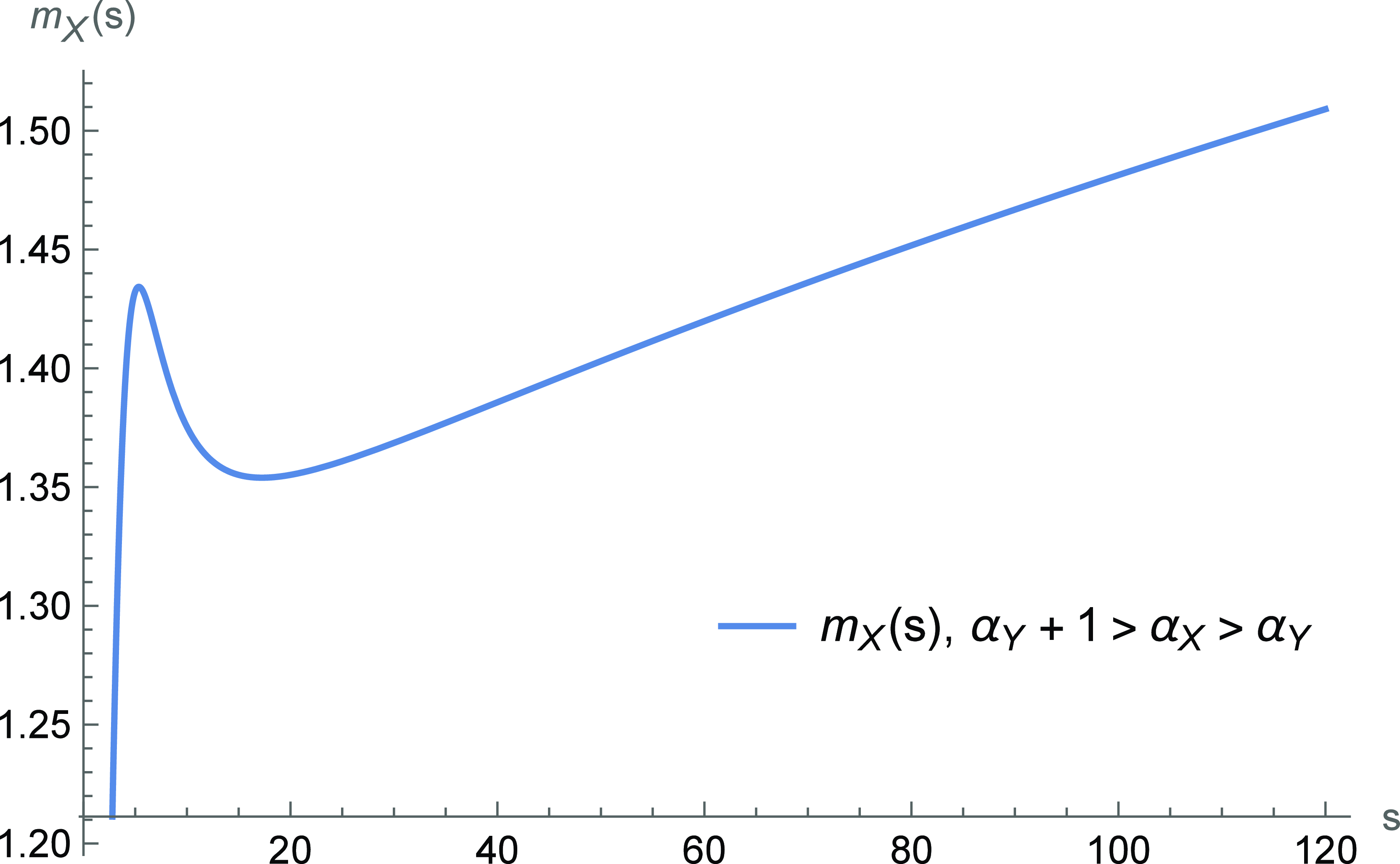
3.3. Boundary case: Difference in tail indices equal to 1 (
$\alpha_X-\alpha_Y=1$
)

The next result shows that when the difference between tail indices is exactly 1, the asymptotic behavior of the conditional expectation given the sum depends on the asymptotic behavior of the ratio between the slowly varying functions associated with the densities.
Proposition 3.10. Let X and Y possess regularly varying densities $f_X(\!\cdot\!)$
and
$f_X(\!\cdot\!)$
and $f_Y(\!\cdot\!)$
with respective indices
$f_Y(\!\cdot\!)$
with respective indices $\alpha _{X}$
and
$\alpha _{X}$
and $\alpha_Y$
verifying
$\alpha_Y$
verifying $\alpha_{X}=\alpha _{Y}+1$
and respective associated slowly varying functions
$\alpha_{X}=\alpha _{Y}+1$
and respective associated slowly varying functions $L_X(\!\cdot\!)$
and
$L_X(\!\cdot\!)$
and $L_Y(\!\cdot\!)$
.
$L_Y(\!\cdot\!)$
.
-
• If
$\frac{L_X(s)}{L_Y(s)}\rightarrow\infty $
as s tends to infinity, then
$m_{X}(s) \rightarrow\infty$
. -
• If
$\lim_{s\rightarrow \infty }\frac{L_X(s)}{L_Y(s)}=k$
with
$k \geq 0$
, then
$\lim_{s\rightarrow \infty }m_{X}(s)=\mathrm{E}[X]+k$
.


Proof. Since $f_X$
is regularly varying with index
$f_X$
is regularly varying with index $\alpha_X\gt3$
, then
$\alpha_X\gt3$
, then $f_{\widetilde{X}}(\!\cdot\!)$
is regularly varying with index
$f_{\widetilde{X}}(\!\cdot\!)$
is regularly varying with index $\alpha_{\widetilde{X}}=\alpha_X-1=\alpha_Y$
. As a consequence of (2.1), taking into account that
$\alpha_{\widetilde{X}}=\alpha_X-1=\alpha_Y$
. As a consequence of (2.1), taking into account that $f_X(\!\cdot\!)$
and
$f_X(\!\cdot\!)$
and $f_Y(\!\cdot\!)$
are regularly varying densities,
$f_Y(\!\cdot\!)$
are regularly varying densities, $f_X(s)=o\left(f_{Y}(s)\right)$
and
$f_X(s)=o\left(f_{Y}(s)\right)$
and $f_{\widetilde{X}}(s)=\frac{s}{\mathrm{E}[X]}f_X(s)$
then
$f_{\widetilde{X}}(s)=\frac{s}{\mathrm{E}[X]}f_X(s)$
then
 \begin{equation} m_X(s)=\mathrm{E}[X] \frac{f_{\widetilde{X}+Y}(s)}{f_{X+Y}(s)}\sim \mathrm{E}[X]\frac{f_{\widetilde{X}}(s)+f_Y(s)}{f_Y(s)+o(f_Y(s))} =\frac{L_X(s)+\mathrm{E}[X] L_Y(s) }{L_Y(s)+o(L_Y(s))}\sim \frac{L_X(s) }{L_Y(s)}+\mathrm{E}[X]. \end{equation}
Hence, if $\frac{L_X(s)}{L_Y(s)}\rightarrow\infty$
as s tends to infinity, it is direct that
$\frac{L_X(s)}{L_Y(s)}\rightarrow\infty$
as s tends to infinity, it is direct that $m_{X}(s)$
diverges. On the other hand, if
$m_{X}(s)$
diverges. On the other hand, if $\lim_{s\rightarrow \infty }\frac{L_X(s)}{L_Y(s)}=k$
with
$\lim_{s\rightarrow \infty }\frac{L_X(s)}{L_Y(s)}=k$
with $k \geq 0$
, from (3.6) then
$k \geq 0$
, from (3.6) then $\lim_{s\rightarrow \infty }m_{X}(s)=\mathrm{E}[X]+k$
.
$\lim_{s\rightarrow \infty }m_{X}(s)=\mathrm{E}[X]+k$
.
The following example illustrates the different cases of Proposition 3.10.
Example 3.11 (Log-Gamma). Consider two independent random variables $X\sim LG(\alpha_X, \lambda_X)$
and
$X\sim LG(\alpha_X, \lambda_X)$
and $Y\sim LG(\alpha_Y, \lambda_Y)$
with
$Y\sim LG(\alpha_Y, \lambda_Y)$
with $\alpha _{X}=\alpha_{Y}+1$
. Here,
$\alpha _{X}=\alpha_{Y}+1$
. Here,
 \begin{equation*} f_X(x)=\frac{(\alpha_X-1)^{\lambda_X}}{\Gamma(\lambda_X)} (\log x)^{\lambda_X-1}x^{-\alpha_X},\hspace{2mm}x\geq 1. \end{equation*}
Then $L_X(x)=\frac{(\alpha_X-1)^{\lambda_X}}{\Gamma(\lambda_X)} (\log x)^{\lambda_X-1}$
and,
$L_X(x)=\frac{(\alpha_X-1)^{\lambda_X}}{\Gamma(\lambda_X)} (\log x)^{\lambda_X-1}$
and,
 \begin{align*} \frac{L_X(x)}{L_Y(x)}=\frac{(\alpha_X-1)^{\lambda_X}}{(\alpha_X-2)^{\lambda_Y}} \frac{\Gamma(\lambda_Y)}{\Gamma(\lambda_X)} (\log x)^{\lambda_X-\lambda_Y}. \end{align*}
Hence, Figure 4 illustrates that in accordance with Proposition 3.10:
Conditional expectation $m_X(\!\cdot\!)$
when
$m_X(\!\cdot\!)$
when $X\sim LG(\alpha_X, \lambda_X)$
and
$X\sim LG(\alpha_X, \lambda_X)$
and $Y\sim LG(\alpha_Y, \lambda_Y)$
with
$Y\sim LG(\alpha_Y, \lambda_Y)$
with $\alpha _{X}=\alpha_{Y}+1$
with
$\alpha _{X}=\alpha_{Y}+1$
with $\alpha_X=5$
,
$\alpha_X=5$
, $\alpha_Y=4$
,
$\alpha_Y=4$
, $\lambda_X=3$
and considering different values of
$\lambda_X=3$
and considering different values of $\lambda_Y$
in each case.
$\lambda_Y$
in each case.
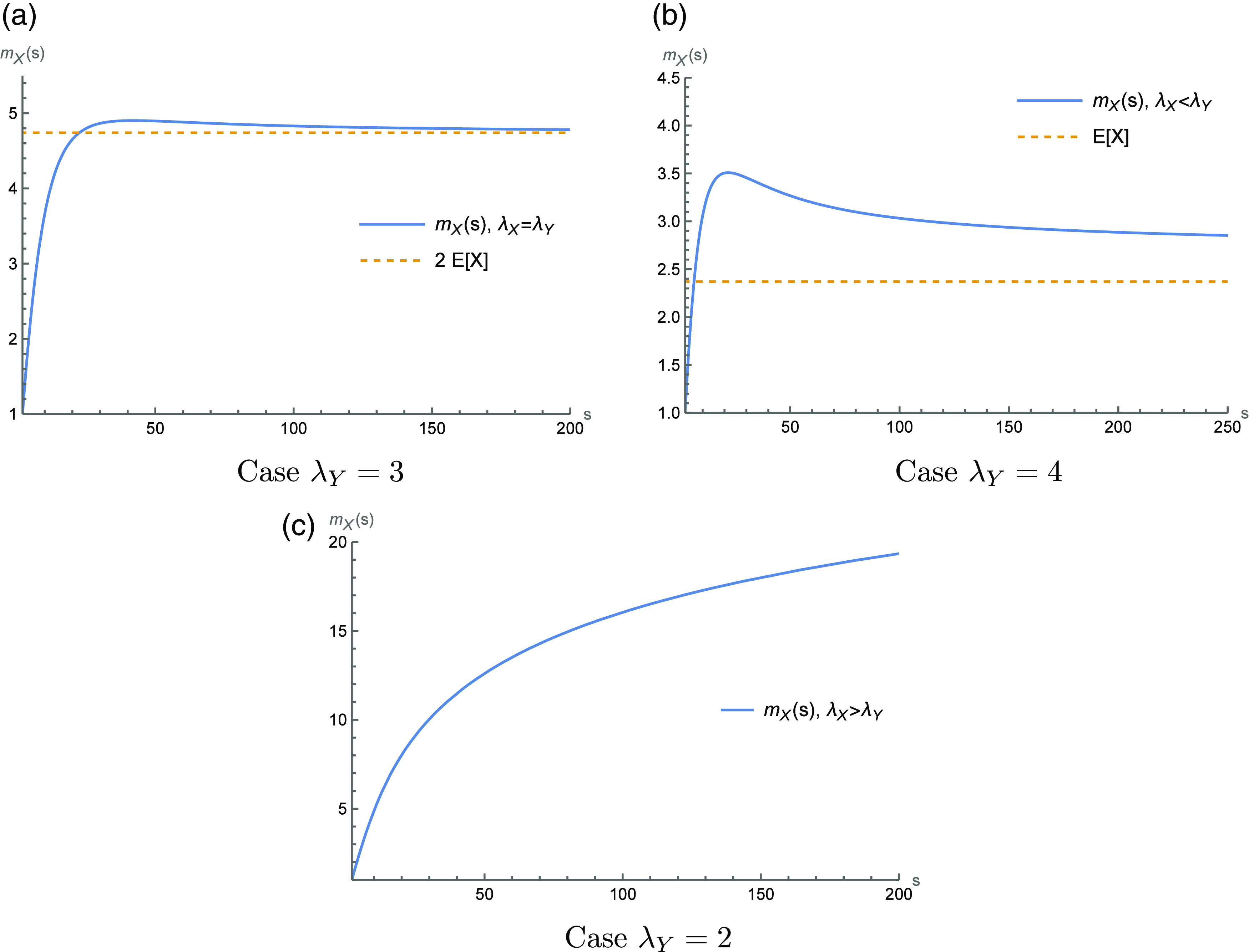
-
• If
$\lambda_X\lt\lambda_Y$
, the latter ratio converges to zero and
$\lim _{s \rightarrow \infty} m_X(s)=\mathrm{E}[X]=\left(\frac{\alpha_X-1}{\alpha_X-2}\right)^{\lambda_X};$
-
• If
$\lambda_X=\lambda_Y$
, then
$\frac{L_X(x)}{L_Y(x)}=\mathrm{E}[X]$
and, therefore,
$\lim _{s \rightarrow \infty} m_X(s)=2 \mathrm{E}[X];$
-
• If
$\lambda_X\gt\lambda_Y$
, the ratio
$\frac{L_X(x)}{L_Y(x)}$
diverges and
$ m_X(s)\rightarrow\infty$
as
$s\rightarrow\infty$
.


Note that in the case where the difference between the tail indices is exactly one and the constant considered in Proposition 3.10 is $k=0$
, similarly to Proposition 3.3, we can ensure that there exists a nonempty interval in
$k=0$
, similarly to Proposition 3.3, we can ensure that there exists a nonempty interval in $(0,\infty)$
where
$(0,\infty)$
where $m_X(\!\cdot\!)$
is decreasing. However, contrary to this case or to the case where the difference in tail indices exceeds 1, there is no guarantee that there exists a nonempty interval of
$m_X(\!\cdot\!)$
is decreasing. However, contrary to this case or to the case where the difference in tail indices exceeds 1, there is no guarantee that there exists a nonempty interval of $(0,\infty)$
where
$(0,\infty)$
where $m_X(\!\cdot\!)$
is decreasing when tail indices differ by one and
$m_X(\!\cdot\!)$
is decreasing when tail indices differ by one and $k\gt0$
. Nevertheless, when the ratio among the slowly varying functions associated with the densities is finite, since the limit is finite,
$k\gt0$
. Nevertheless, when the ratio among the slowly varying functions associated with the densities is finite, since the limit is finite, $m_X(\!\cdot\!)$
is necessarily bounded. Under this framework, we can now encounter a variety of different behaviors for
$m_X(\!\cdot\!)$
is necessarily bounded. Under this framework, we can now encounter a variety of different behaviors for $m_X(\!\cdot\!)$
, as illustrated in Example 3.12. In the first situation considered there, the conditional expectation given the sum is monotonically increasing over an interval (0,b) for a large b. However, in the second situation, the conditional expectation given the sum peaks before decreasing to tend to its limit from above.
$m_X(\!\cdot\!)$
, as illustrated in Example 3.12. In the first situation considered there, the conditional expectation given the sum is monotonically increasing over an interval (0,b) for a large b. However, in the second situation, the conditional expectation given the sum peaks before decreasing to tend to its limit from above.
Example 3.12. Let us consider two independent random variables $X\sim P(I)(\theta, \alpha_{X})$
and
$X\sim P(I)(\theta, \alpha_{X})$
and $Y\sim P(I)(\theta, \alpha _{Y})$
such that
$Y\sim P(I)(\theta, \alpha _{Y})$
such that $\alpha _{X}=\alpha_{Y}+1$
. Then,
$\alpha _{X}=\alpha_{Y}+1$
. Then, $\widetilde{X}\sim P(I)(\theta, \alpha _{X}-1)$
so that
$\widetilde{X}\sim P(I)(\theta, \alpha _{X}-1)$
so that $\widetilde{X}\overset{\mathrm{d}}{=} Y$
, where
$\widetilde{X}\overset{\mathrm{d}}{=} Y$
, where $\overset{\mathrm{d}}{=}$
stands for “equally distributed”. Note that
$\overset{\mathrm{d}}{=}$
stands for “equally distributed”. Note that $ k=\mathrm{E}[X]$
in Proposition 3.10, and from Proposition 3.10,
$ k=\mathrm{E}[X]$
in Proposition 3.10, and from Proposition 3.10, $\lim_{s\rightarrow \infty }m_X(s)=2\mathrm{E}[X]$
. However, the behavior of
$\lim_{s\rightarrow \infty }m_X(s)=2\mathrm{E}[X]$
. However, the behavior of $m_X(\!\cdot\!)$
differs according to the value of
$m_X(\!\cdot\!)$
differs according to the value of $\alpha_Y$
, as shown in the two following situations:
$\alpha_Y$
, as shown in the two following situations:
-
1. Figure 5 shows that there are situations where
$m_X(\!\cdot\!)$
increases over (0,50) and, numerically, we observe that it tends to its limit from below.Figure 5.Conditional expectation
$m_X(\!\cdot\!)$
(blue solid line) and horizontal line at
$2\mathrm{E}[X]$
(orange dashed line) when
$X\sim P(I)(\theta, \alpha_X )$
and
$Y\sim P(I)(\theta, \alpha_Y )$
with
$\theta =1$
,
$\alpha_X =6$
and
$\alpha_Y =5$
. -
2. Figure 6 shows that there are situations where
$m_X(\!\cdot\!)$
attains a maximum before decreasing to its limit. Specifically, we can see there that, considering the values
$\theta =1$
,
$\alpha_X =3.5$
and
$\alpha_Y =2.5$
,
$m_X(\!\cdot\!)$
increases over
$(0,64.46)$
where
$64.46\simeq F^{-1}(0.998)$
and then decreases over
$(64.46,1000)$
. From the plot, we conjecture that it tends to its limit from above.Figure 6.Conditional expectation
$m_X(\!\cdot\!)$
(blue solid line) and horizontal line at
$2\mathrm{E}[X]$
(orange dashed line) when
$X\sim P(I)(\theta, \alpha_X )$
and
$Y\sim P(I)(\theta, \alpha_Y )$
with
$\theta =1$
,
$\alpha_X =3.5$
, and
$\alpha_Y =2.5$
.


From this section, we can conclude that if the difference between the indices exceeds one, $m_X(\!\cdot\!)$
will decrease in an interval; if the difference is less than one,
$m_X(\!\cdot\!)$
will decrease in an interval; if the difference is less than one, $m_X(\!\cdot\!)$
diverges; and in the boundary case (i.e. if the difference is exactly one) it can be either bounded or not, depending on the asymptotic behavior of the ratio between the associated slowly varying functions.
$m_X(\!\cdot\!)$
diverges; and in the boundary case (i.e. if the difference is exactly one) it can be either bounded or not, depending on the asymptotic behavior of the ratio between the associated slowly varying functions.
In the following section, in addition to the asymptotic levels, we aim to delve into the rate at which $m_X(\!\cdot\!)$
is either converging or diverging as the argument gets larger.
$m_X(\!\cdot\!)$
is either converging or diverging as the argument gets larger.
4. Asymptotic behavior of the conditional mean given the sum
The asymptotic levels of the conditional expectation given the sum were discussed in the preceding section. In this section, we supplement these results with the asymptotic behavior of $m_X(\!\cdot\!)$
and illustrate the accuracy of the resulting approximations with various examples.
$m_X(\!\cdot\!)$
and illustrate the accuracy of the resulting approximations with various examples.
4.1. Asymptotic expansion of the conditional mean given the sum
Define the truncated mean function for a nonnegative random variable Z as
 \begin{equation}\mu_{Z}\left( t\right) =\int_{0}^{t}xf_{Z}\left( x\right) \mathrm{d} x.\end{equation}
If the expectation is finite (i.e. $\alpha _{Z}\gt2$
), the truncated mean tends to the expected value, which is denoted by
$\alpha _{Z}\gt2$
), the truncated mean tends to the expected value, which is denoted by $\mu_Z$
:
$\mu_Z$
:
 \begin{equation*}\lim_{t\rightarrow \infty }\mu_{Z}\left( t\right) =\mu_{Z}=\mathrm{E}[Z]\lt\infty.\end{equation*}
The variance of Z will be denoted by $\sigma^2_Z$
. The following result provides an asymptotic expansion of the density function of the sum
$\sigma^2_Z$
. The following result provides an asymptotic expansion of the density function of the sum $X+Y$
when X and Y both possess asymptotically smooth densities. This is an extension of Theorem 1.1 in Bingham et al. (Reference Bingham, Goldie and Omey2006).
$X+Y$
when X and Y both possess asymptotically smooth densities. This is an extension of Theorem 1.1 in Bingham et al. (Reference Bingham, Goldie and Omey2006).
Proposition 4.1. Let X and Y be positive random variables with asymptotically smooth density functions $f_{X}(\!\cdot\!)$
and
$f_{X}(\!\cdot\!)$
and $f_{Y}(\!\cdot\!)$
with tail indices
$f_{Y}(\!\cdot\!)$
with tail indices $\alpha _{X}$
and
$\alpha _{X}$
and $\alpha _{Y}$
such that
$\alpha _{Y}$
such that $\min\{\alpha _{X},\alpha _{Y}\}\geq2$
. Then, as s tends to infinity,
$\min\{\alpha _{X},\alpha _{Y}\}\geq2$
. Then, as s tends to infinity,
 \begin{equation*}f_{X+Y}\left( s\right) =f_{X}\left( s\right) \left( 1+\alpha _{X}\frac{\mu_{Y}\left( s\right) }{s}\left( 1+o\left( 1\right) \right) \right)+f_{Y}\left( s\right) \left( 1+\alpha _{Y}\frac{\mu _{X}\left( s\right) }{s}\left( 1+o\left( 1\right) \right) \right) .\end{equation*}
In particular, if $\min\{\alpha _{X},\alpha _{Y}\}\gt2$
,
$\min\{\alpha _{X},\alpha _{Y}\}\gt2$
,
 \begin{equation*} f_{X+Y}\left( s\right) =f_{X}\left( s\right) \left( 1+\alpha _{X}\frac{\mu _{Y} }{s}\left( 1+o\left( 1\right) \right) \right) +f_{Y}\left( s\right) \left( 1+\alpha _{Y}\frac{\mu _{X} }{s} \left( 1+o\left( 1\right) \right) \right) .\end{equation*}
Proof. The density function of $X+Y$
can be written as
$X+Y$
can be written as
 \begin{equation*}f_{X+Y}\left( t\right) =\int_{0}^{t}f_{X}\left( t-x\right) f_{Y}\left(x\right) \mathrm{d} x=T_{Y}f_{X}\left( t\right) +T_{X}f_{Y}\left( t\right)\end{equation*}
where
 \begin{equation*}T_{Y}f_{X}\left( t\right) =\int_{0}^{t/2}f_{X}\left( t-x\right) f_{Y}\left(x\right) \mathrm{d} x.\end{equation*}
The announced result then follows from the expressions for $T_{Y}f_{X}\left( t\right)$
and
$T_{Y}f_{X}\left( t\right)$
and $T_{X}f_{Y}\left( t\right)$
derived in Proposition B.1 in Appendix B.
$T_{X}f_{Y}\left( t\right)$
derived in Proposition B.1 in Appendix B.
An asymptotic expansion for the conditional mean given the sum is then deduced from this result.
Proposition 4.2. Let X and Y be positive random variables with asymptotically smooth density functions $f_{X}(\!\cdot\!)$
and
$f_{X}(\!\cdot\!)$
and $f_{Y}(\!\cdot\!)$
with tail indices
$f_{Y}(\!\cdot\!)$
with tail indices $\alpha _{X}$
and
$\alpha _{X}$
and $\alpha _{Y}$
such that
$\alpha _{Y}$
such that $\min\{\alpha _{X}-1,\alpha _{Y}\}\gt2$
. Then, as s tends to infinity,
$\min\{\alpha _{X}-1,\alpha _{Y}\}\gt2$
. Then, as s tends to infinity,
 \begin{equation}m_{X}(s)=\frac{f_{X}\left( s\right) \left( s+(\alpha _{X}-1)\mu _{Y}\big(1+o\left( 1\right) \big) \right)+\mu _{X}f_{Y}\left( s\right) \left(1+\frac{\alpha _{Y}\mu _{\widetilde{X}}}{s}\big( 1+o\left( 1\right) \big) \right)}{f_{X}\left( s\right) \left( 1+\frac{\alpha _{X}\mu _{Y}}{s}\big( 1+o\left(1\right) \big) \right)+f_{Y}\left( s\right) \left( 1+\frac{\alpha_{Y}\mu _{X}}{s}\big( 1+o\left( 1\right) \big) \right) }.\end{equation}
Proof. Representation (2.2) shows that $m_{X}(\!\cdot\!)$
can be expressed with the help of the ratio of the densities of
$m_{X}(\!\cdot\!)$
can be expressed with the help of the ratio of the densities of $\widetilde{X}+Y$
of
$\widetilde{X}+Y$
of $X+Y$
. Applying Proposition 4.1 to these densities, and taking into account that
$X+Y$
. Applying Proposition 4.1 to these densities, and taking into account that $\alpha_{\widetilde{X}}=\alpha_X-1\gt2$
, we get
$\alpha_{\widetilde{X}}=\alpha_X-1\gt2$
, we get
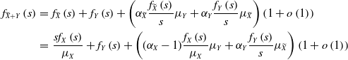 \begin{eqnarray*} f_{\widetilde{X}+Y}\left( s\right) &=&f_{\widetilde{X}}\left( s\right)+f_{Y}\left( s\right)+\left( \alpha_{\widetilde{X}} \frac{f_{\widetilde{X}}\left( s\right)}{s}\mu _{Y}+\alpha_Y \frac{f_{Y}\left( s\right) }{s}\mu _{\widetilde{X}}\right) \left( 1+o\left( 1\right) \right)\\&=&\frac{sf_{X}\left( s\right)}{\mu_X}+f_{Y}\left( s\right)+\left( (\alpha_X-1) \frac{f_{X}\left( s\right)}{\mu_X}\mu _{Y}+\alpha_Y \frac{f_{Y}\left( s\right) }{s}\mu _{\widetilde{X}}\right) \left( 1+o\left( 1\right) \right)\end{eqnarray*}
and
 \begin{equation*} f_{X+Y}\left( s\right) =f_{X}\left( s\right)+f_{Y}\left( s\right)+\left( \alpha_X \frac{f_{X}\left( s\right)}{s}\mu _{Y}+\alpha_Y \frac{f_{Y}\left( s\right) }{s}\mu _{X}\right) \left( 1+o\left( 1\right) \right)\end{equation*}
as s tends to infinity. The announced result then follows from (2.2).
Proposition 4.2 allows us to study the asymptotic behavior of the conditional expectation given the sum according to the values of the tail indices. In the following sections, we will study it under different frameworks and we assume again that $\alpha_{X}\geq \alpha_Y$
. Note that, if
$\alpha_{X}\geq \alpha_Y$
. Note that, if $\alpha_Y\gt\alpha_X$
, the asymptotic expression of
$\alpha_Y\gt\alpha_X$
, the asymptotic expression of $m_X(\!\cdot\!)$
can be obtained by computing the asymptotic expression of
$m_X(\!\cdot\!)$
can be obtained by computing the asymptotic expression of $m_Y(\!\cdot\!)$
and noting that
$m_Y(\!\cdot\!)$
and noting that $m_{X}(s)=s-m_Y(s)$
. Although it must be noted that, in order to obtain the asymptotic expression of
$m_{X}(s)=s-m_Y(s)$
. Although it must be noted that, in order to obtain the asymptotic expression of $m_X\left(\cdot\right)$
, it is required that
$m_X\left(\cdot\right)$
, it is required that $\alpha_X\gt3$
and
$\alpha_X\gt3$
and $\alpha_Y\gt2$
. Hence, if computing the asymptotic expression of
$\alpha_Y\gt2$
. Hence, if computing the asymptotic expression of $m_Y\left(\cdot\right)$
, we need to assume
$m_Y\left(\cdot\right)$
, we need to assume $\alpha_Y\gt3$
and
$\alpha_Y\gt3$
and $\alpha_X\gt2$
.
$\alpha_X\gt2$
.
Based on Proposition 4.2, we derive different types of asymptotic behaviors of the conditional mean of X given the sum, as detailed in the next sections. We consider two cases where $m_X\left(\cdot\right)$
converges to the unconditional expected value: when the difference of the indices is greater than two and when it is in between one and two. In addition, we compare the asymptotic behavior of
$m_X\left(\cdot\right)$
converges to the unconditional expected value: when the difference of the indices is greater than two and when it is in between one and two. In addition, we compare the asymptotic behavior of $m_X\left(\cdot\right)$
as it diverges, by deriving the asymptotic expansion when indices are “near” (their difference is positive but smaller than one) and when both variables have the same index. Figure 7 illustrates the different cases considered in the next sections within the plane
$m_X\left(\cdot\right)$
as it diverges, by deriving the asymptotic expansion when indices are “near” (their difference is positive but smaller than one) and when both variables have the same index. Figure 7 illustrates the different cases considered in the next sections within the plane $( \alpha _{X},\alpha_{Y})$
. As is common to the different cases, throughout the next sections, we will assume
$( \alpha _{X},\alpha_{Y})$
. As is common to the different cases, throughout the next sections, we will assume $\alpha_X\gt3$
and
$\alpha_X\gt3$
and $\alpha_Y\gt2$
. In the following sections, we will denote by
$\alpha_Y\gt2$
. In the following sections, we will denote by $\widehat{m}_X\left(\cdot\right)$
an approximation of
$\widehat{m}_X\left(\cdot\right)$
an approximation of $m_X\left(\cdot\right)$
at infinity.
$m_X\left(\cdot\right)$
at infinity.
Discussion according to the position of $( \alpha _{X},\alpha_{Y})$
in
$( \alpha _{X},\alpha_{Y})$
in $(3,\infty)\times(2,\infty)$
with
$(3,\infty)\times(2,\infty)$
with $\alpha_{X}\geq \alpha_Y$
.
$\alpha_{X}\geq \alpha_Y$
.

4.2. Difference in the tail indices larger than 2 (
$\alpha_X-\alpha_Y\gt2$
)

From Proposition 4.2, we can write $m_X\left(\cdot\right)$
as the ratio of two asymptotic expansions, each considering four terms. Note that, assuming
$m_X\left(\cdot\right)$
as the ratio of two asymptotic expansions, each considering four terms. Note that, assuming $\alpha_X-\alpha_Y\gt1$
, the terms of the denominator are regularly varying with arranged indices
$\alpha_X-\alpha_Y\gt1$
, the terms of the denominator are regularly varying with arranged indices $\lbrace \alpha_Y, \alpha_Y+1,\alpha_X,\alpha_X+1 \rbrace$
. Therefore,
$\lbrace \alpha_Y, \alpha_Y+1,\alpha_X,\alpha_X+1 \rbrace$
. Therefore, $\alpha_Y$
and
$\alpha_Y$
and $\alpha_Y+1$
are the two smallest indices (i.e., the two greatest orders). With respect to the numerator, the (non-arranged) indices of the terms are
$\alpha_Y+1$
are the two smallest indices (i.e., the two greatest orders). With respect to the numerator, the (non-arranged) indices of the terms are $\lbrace \alpha_X-1,\alpha_X, \alpha_Y, \alpha_Y+1 \rbrace$
. Under the assumption
$\lbrace \alpha_X-1,\alpha_X, \alpha_Y, \alpha_Y+1 \rbrace$
. Under the assumption $\alpha_X-\alpha_Y\gt1$
, the smallest index is
$\alpha_X-\alpha_Y\gt1$
, the smallest index is $\alpha_Y$
. However, if
$\alpha_Y$
. However, if $\alpha_X-\alpha_Y\gt2$
, the second smallest index is
$\alpha_X-\alpha_Y\gt2$
, the second smallest index is $\alpha_Y+1$
and, if
$\alpha_Y+1$
and, if $\alpha_X-\alpha_Y\lt2$
, it is
$\alpha_X-\alpha_Y\lt2$
, it is $\alpha_X-1$
. This motivates the study of the behavior of
$\alpha_X-1$
. This motivates the study of the behavior of $m_X\left(\cdot\right)$
separately if the difference between indices trespasses two.
$m_X\left(\cdot\right)$
separately if the difference between indices trespasses two.
Proposition 4.3. Let X and Y be positive random variables possessing asymptotically smooth density functions $f_X(\!\cdot\!)$
and
$f_X(\!\cdot\!)$
and $f_Y(\!\cdot\!)$
with respective tail indices
$f_Y(\!\cdot\!)$
with respective tail indices $\alpha _{X}$
and
$\alpha _{X}$
and $\alpha _{Y}$
. If
$\alpha _{Y}$
. If $\alpha _{X}\gt\alpha _{Y}+2$
, then
$\alpha _{X}\gt\alpha _{Y}+2$
, then
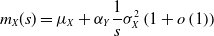 \begin{equation*}m_{X}(s)=\mu _{X}+\alpha _{Y}\frac{1}{s}\sigma^2_X\left( 1+o\left( 1\right) \right)\end{equation*}
as s tends to infinity.
Proof. Notice that $\sigma^2_X=\mu_{\widetilde{X}}\mu_{X}-\mu_{X}^2.$
Since
$\sigma^2_X=\mu_{\widetilde{X}}\mu_{X}-\mu_{X}^2.$
Since $\min\{\alpha _{X}-1,\alpha _{Y}\}\gt2$
, (4.2) allows us to write
$\min\{\alpha _{X}-1,\alpha _{Y}\}\gt2$
, (4.2) allows us to write
 \begin{equation*}m_{X}(s)=\frac{sf_{X}\left( s\right) +\mu _{X}f_{Y}\left( s\right)+\left( (\alpha_X -1)f_{X}\left( s\right)\mu _{Y}+\alpha_Y \frac{f_{Y}\left( s\right) }{s}\left(\sigma^2_X+\mu _{X}^2\right)\right) \left( 1+o\left( 1\right) \right)}{ f_{X}\left( s\right)+f_{Y}\left( s\right)+\left( \alpha_X \frac{f_{X}\left( s\right)}{s}\mu _{Y}+\alpha_Y \frac{f_{Y}\left( s\right) }{s}\mu _{X}\right) \left( 1+o\left( 1\right) \right)}\end{equation*}
as s tends to infinity. As $\alpha _{Y}\gt2$
and
$\alpha _{Y}\gt2$
and $\alpha _{X}\gt\alpha _{Y}+2$
, we have that
$\alpha _{X}\gt\alpha _{Y}+2$
, we have that $f_{X}\left( s\right) =o(\frac{f_{Y}\left( s\right) }{s^2})$
, and we can write
$f_{X}\left( s\right) =o(\frac{f_{Y}\left( s\right) }{s^2})$
, and we can write
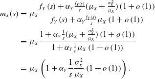 \begin{eqnarray*}m_{X}(s) &=&\mu _{X}\frac{f_{Y}\left( s\right)+\alpha _{Y}\frac{f_{Y}\left( s\right) }{s}(\mu _{X}+\frac{\sigma^2_X}{ \mu _{X}})\left(1+o\left( 1\right) \right) }{f_{Y}\left( s\right) +\alpha _{Y}\frac{f_{Y}\left( s\right) }{s}\mu _{X}\left( 1+o\left( 1\right) \right) } \\&=&\mu _{X}\frac{1+\alpha _{Y}\frac{1}{s}(\mu _{X}+\frac{\sigma^2_X}{\mu _{X}})\left( 1+o\left( 1\right) \right) }{1+\alpha _{Y}\frac{1}{s}\mu_{X}\left( 1+o\left( 1\right) \right) } \\&& \\&=&\mu _{X}\left( 1+\alpha _{Y}\frac{1}{s}\frac{\sigma^2_X}{\mu _{X}}\left( 1+o\left( 1\right) \right) \right) .\end{eqnarray*}
This ends the proof.
The following example illustrates Proposition 4.3.
Example 4.4. Let us consider two independent random variables $X\sim P(II)(\theta, \alpha_{X},\vartheta)$
and
$X\sim P(II)(\theta, \alpha_{X},\vartheta)$
and $Y\sim P(II)(\theta, \alpha _{Y},\vartheta)$
such that
$Y\sim P(II)(\theta, \alpha _{Y},\vartheta)$
such that $\alpha _{X}=10$
,
$\alpha _{X}=10$
, $\alpha_Y=5$
,
$\alpha_Y=5$
, $\theta=1$
, and
$\theta=1$
, and $\vartheta=0$
. Figure 8 shows the same asymptotic behavior of
$\vartheta=0$
. Figure 8 shows the same asymptotic behavior of $m_X(\!\cdot\!)$
and
$m_X(\!\cdot\!)$
and $\widehat{m}_X(s)=\mu _{X}\left( 1+\alpha _{Y}\frac{1}{s}\frac{\sigma^2_X}{\mu _{X}}\right)$
.
$\widehat{m}_X(s)=\mu _{X}\left( 1+\alpha _{Y}\frac{1}{s}\frac{\sigma^2_X}{\mu _{X}}\right)$
.
Conditional expectation $m_X(\!\cdot\!)$
when
$m_X(\!\cdot\!)$
when $X\sim P(II)(\theta, \alpha_{X},\vartheta)$
and
$X\sim P(II)(\theta, \alpha_{X},\vartheta)$
and $Y\sim P(II)(\theta, \alpha _{Y},\vartheta)$
with
$Y\sim P(II)(\theta, \alpha _{Y},\vartheta)$
with $\alpha _{X}=10$
,
$\alpha _{X}=10$
, $\alpha_Y=5$
,
$\alpha_Y=5$
, $\theta=1$
, and
$\theta=1$
, and $\vartheta=0$
.
$\vartheta=0$
.
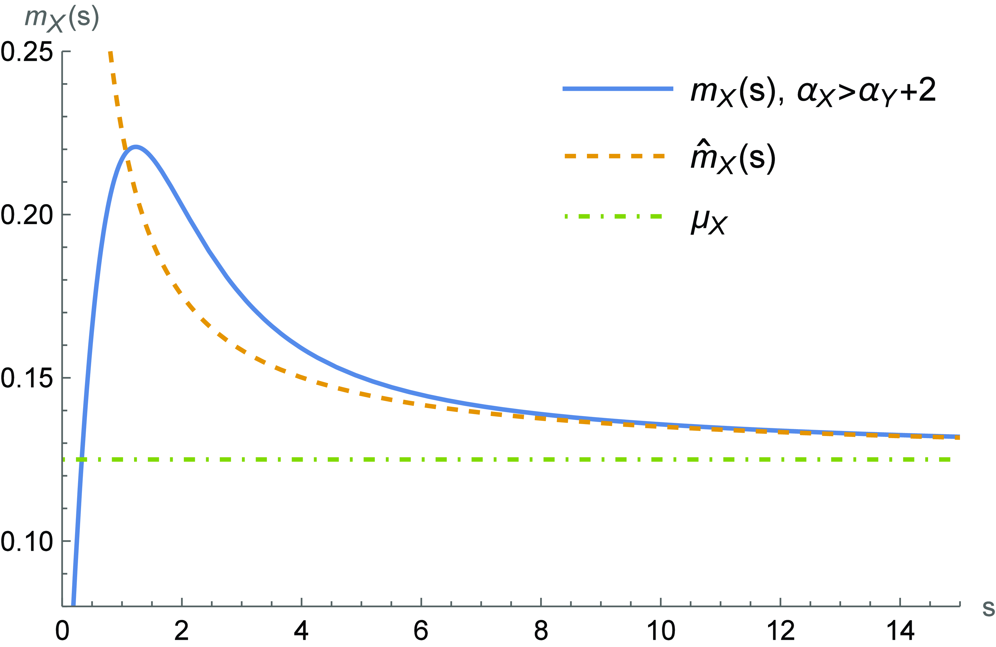
4.3. Difference in the tail indices between 1 and 2 (
$1 \lt \alpha_X-\alpha_Y \lt 2$
)

Proposition 4.5. Let X and Y be positive random variables possessing asymptotically smooth density functions $f_X(\!\cdot\!)$
and
$f_X(\!\cdot\!)$
and $f_Y(\!\cdot\!)$
with respective tail indices
$f_Y(\!\cdot\!)$
with respective tail indices $\alpha _{X}$
and
$\alpha _{X}$
and $\alpha _{Y}$
. If
$\alpha _{Y}$
. If $\alpha_Y+2\gt\alpha _{X}\gt\alpha _{Y}+1$
, then
$\alpha_Y+2\gt\alpha _{X}\gt\alpha _{Y}+1$
, then
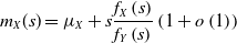 \begin{equation*}m_{X}(s)=\mu _{X}+s\frac{f_{X}\left( s\right) }{f_{Y}\left(s\right) }\left( 1+o\left( 1\right) \right)\end{equation*}
as s tends to infinity.
Proof. Since $\alpha _{Y}\gt2$
and
$\alpha _{Y}\gt2$
and $\alpha _{Y}+2\gt \alpha _{X}\gt\alpha_{Y}+1$
, we have that
$\alpha _{Y}+2\gt \alpha _{X}\gt\alpha_{Y}+1$
, we have that $f_{X}\left( s\right) =o\left(\frac{f_{Y}\left( s\right)}{s}\right)$
and
$f_{X}\left( s\right) =o\left(\frac{f_{Y}\left( s\right)}{s}\right)$
and $ \frac{f_{Y}\left( s\right)}{s} =o(sf_{X}\left( s\right) )$
. Hence, we can write
$ \frac{f_{Y}\left( s\right)}{s} =o(sf_{X}\left( s\right) )$
. Hence, we can write
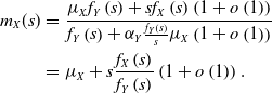 \begin{eqnarray*}m_{X}(s) &=&\frac{\mu _{X}f_{Y}\left( s\right) +sf_{X}\left( s\right) \left( 1+o\left( 1\right) \right) }{f_{Y}\left(s\right) +\alpha _{Y}\frac{f_{Y}\left( s\right) }{s}\mu _{X}\left( 1+o\left(1\right) \right) } \\&=&\mu _{X}+s\frac{f_{X}\left( s\right) }{f_{Y}\left(s\right) }\left( 1+o\left( 1\right) \right).\end{eqnarray*}
This ends the proof.
The following example illustrates Proposition 4.5
Example 4.6. Let us consider two independent random variables $X\sim Davis(\alpha_{X},b,\vartheta)$
and
$X\sim Davis(\alpha_{X},b,\vartheta)$
and $Y\sim Davis(\alpha _{Y},b,\vartheta)$
such that
$Y\sim Davis(\alpha _{Y},b,\vartheta)$
such that $\alpha _{X}=6$
,
$\alpha _{X}=6$
, $\alpha_Y=4.5$
,
$\alpha_Y=4.5$
, $b=2$
, and
$b=2$
, and $\vartheta=0$
. Figure 9 shows the same asymptotic behavior of
$\vartheta=0$
. Figure 9 shows the same asymptotic behavior of $m_X(\!\cdot\!)$
and
$m_X(\!\cdot\!)$
and $\widehat{m}_X(s)=\mu _{X}+s\frac{f_{X}\left( s\right) }{f_{Y}\left(s\right) }$
.
$\widehat{m}_X(s)=\mu _{X}+s\frac{f_{X}\left( s\right) }{f_{Y}\left(s\right) }$
.
Conditional expectation $m_X(\!\cdot\!)$
when
$m_X(\!\cdot\!)$
when $X\sim Davis(\alpha_{X},b,\vartheta)$
and
$X\sim Davis(\alpha_{X},b,\vartheta)$
and $Y\sim Davis(\alpha _{Y},b,\vartheta)$
with
$Y\sim Davis(\alpha _{Y},b,\vartheta)$
with $\alpha _{X}=6$
,
$\alpha _{X}=6$
, $\alpha_Y=4.5$
,
$\alpha_Y=4.5$
, $b=2$
, and
$b=2$
, and $\vartheta=0$
.
$\vartheta=0$
.

From Proposition 4.3, if $\alpha_X-\alpha_Y\gt2$
, the asymptotic behavior of
$\alpha_X-\alpha_Y\gt2$
, the asymptotic behavior of $m_X\left(\cdot\right)$
can be approximated by
$m_X\left(\cdot\right)$
can be approximated by $\widehat{m}_{X}(s)=\mu _{X}+\alpha_{Y}\frac{1}{s}\sigma^2_X$
, where the second term behaves proportionally to
$\widehat{m}_{X}(s)=\mu _{X}+\alpha_{Y}\frac{1}{s}\sigma^2_X$
, where the second term behaves proportionally to $1/s$
. However, if
$1/s$
. However, if $1\lt\alpha_X-\alpha_Y\lt2$
, by Proposition 4.5, asymptotically,
$1\lt\alpha_X-\alpha_Y\lt2$
, by Proposition 4.5, asymptotically, $m_X\left(\cdot\right)$
can be approximated by
$m_X\left(\cdot\right)$
can be approximated by $\widehat{m}_{X}(s)=\mu _{X}+s\frac{f_{X}\left( s\right) }{f_{Y}\left(s\right)}$
, whose second term is
$\widehat{m}_{X}(s)=\mu _{X}+s\frac{f_{X}\left( s\right) }{f_{Y}\left(s\right)}$
, whose second term is $s^{-\alpha_X+1+\alpha_Y}\frac{L_{X}\left( s\right) }{L_{Y}\left(s\right)}$
. Note that
$s^{-\alpha_X+1+\alpha_Y}\frac{L_{X}\left( s\right) }{L_{Y}\left(s\right)}$
. Note that $-\alpha_X+1+\alpha_Y\gt-1$
. Hence, as we could expect, if
$-\alpha_X+1+\alpha_Y\gt-1$
. Hence, as we could expect, if $\alpha_X-\alpha_Y\gt2$
, asymptotically,
$\alpha_X-\alpha_Y\gt2$
, asymptotically, $m_X\left(\cdot\right)$
decreases faster as it does if
$m_X\left(\cdot\right)$
decreases faster as it does if $1\lt\alpha_X-\alpha_Y\lt2$
.
$1\lt\alpha_X-\alpha_Y\lt2$
.
4.4. Difference in the tail indices less than 1 (
$0 \lt \alpha_X-\alpha_Y \lt 1$
)

When the indices are similar, and by similar, we mean here that they do not differ by more than one unit, the following result provides the asymptotic expression of $m_X\left(\cdot\right)$
, where the second and third terms vary depending on how similar are the indices. Note that the expressions are arranged in terms of their order, so even if the terms considered are the same in the two first cases, they are given separately to emphasize that the second-order term differs in the two cases.
$m_X\left(\cdot\right)$
, where the second and third terms vary depending on how similar are the indices. Note that the expressions are arranged in terms of their order, so even if the terms considered are the same in the two first cases, they are given separately to emphasize that the second-order term differs in the two cases.
Proposition 4.7. Let X and Y be positive random variables possessing asymptotically smooth density functions $f_X(\!\cdot\!)$
and
$f_X(\!\cdot\!)$
and $f_Y(\!\cdot\!)$
with respective tail indices
$f_Y(\!\cdot\!)$
with respective tail indices $\alpha _{X}$
and
$\alpha _{X}$
and $\alpha _{Y}$
. If
$\alpha _{Y}$
. If $\alpha_Y+1\gt\alpha _{X}\gt\alpha _{Y}$
then, as s tends to infinity:
$\alpha_Y+1\gt\alpha _{X}\gt\alpha _{Y}$
then, as s tends to infinity:
-
(a) if
$1\gt\alpha_X-\alpha_Y\gt\frac{1}{2}$
, then:
\begin{equation*} m_{X}(s)=s\frac{f_X(s) }{f_Y(s)}\left(1+\mu_{X}\frac{f_Y(s) }{s f_X(s)}-\frac{f_X(s) }{f_Y(s)}(1+o(1))\right);\end{equation*}
-
(b) if
$\frac{1}{2}\gt\alpha_X-\alpha_Y\gt\frac{1}{3}$
, then:
\begin{equation*} m_{X}(s)=s\frac{f_X(s) }{f_Y(s)}\left(1-\frac{f_X(s) }{f_Y(s)}+\mu_{X}\frac{f_Y(s) }{s f_X(s)}(1+o(1))\right);\end{equation*}
-
(c) if
$\frac{1}{3}\gt\alpha_X-\alpha_Y\gt0$
, then:
\begin{equation*} m_{X}(s)=s\frac{f_X(s) }{f_Y(s)}\left(1-\frac{f_X(s) }{f_Y(s)}+\left(\frac{f_X(s) }{f_Y(s)}\right)^2(1+o(1))\right)\end{equation*}


Proof. If $\alpha _{Y}+1\gt\alpha _{X}\gt\alpha _{Y}$
, since
$\alpha _{Y}+1\gt\alpha _{X}\gt\alpha _{Y}$
, since $\alpha_X\gt3$
and
$\alpha_X\gt3$
and $\alpha_Y\gt2$
, then, as s tends to infinity:
$\alpha_Y\gt2$
, then, as s tends to infinity:
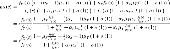 \begin{eqnarray*} m_{X}(s)&=&\frac{f_{X}\left( s\right) \big( s+(\alpha _{X}-1)\mu _{Y}\left( 1+o\left( 1\right) \right) \big) +\mu _{X}f_{Y}\left( s\right) \big( 1+\alpha _{Y}\mu _{\widetilde{X}}s^{-1}\left( 1+o\left( 1\right) \right) \big) }{ f_{X}\left( s\right) \big( 1+\alpha _{X}\mu _{Y}s^{-1}\left( 1+o\left( 1\right) \right) \big) +f_{Y}\left( s\right) \big( 1+\alpha _{Y}\mu _{X}s^{-1}\left( 1+o\left( 1\right) \right)\big) }\\ &=&s\frac{f_{X}\left( s\right)}{f_{Y}\left( s\right)}\frac{ 1+\mu _{X}\frac{f_{Y}\left( s\right)}{s f_{X}\left( s\right)}+\frac{1}{s}(\alpha _{X}-1)\mu _{Y}\left( 1+o\left( 1\right) \right) +\alpha _{Y}\mu _{\widetilde{X}}\mu _{X}\frac{f_{Y}\left( s\right)}{s^2 f_{X}\left( s\right)} \left( 1+o\left( 1\right) \right) }{ 1+\frac{f_{X}\left( s\right)}{f_{Y}\left( s\right)}+\alpha _{Y}\mu _{X}\frac{1}{s}\left( 1+o\left( 1\right) \right) +\alpha _{X}\mu _{Y} \frac{f_{X}\left( s\right)}{s f_{Y}\left( s\right)}\left( 1+o\left( 1\right) \right) }\\ &=&s\frac{f_{X}\left( s\right)}{f_{Y}\left( s\right)}\frac{ 1+\mu _{X}\frac{f_{Y}\left( s\right)}{s f_{X}\left( s\right)}+\frac{1}{s}(\alpha _{X}-1)\mu _{Y}\left( 1+o\left( 1\right) \right) }{ 1+\frac{f_{X}\left( s\right)}{f_{Y}\left( s\right)}+\alpha _{Y}\mu _{X}\frac{1}{s}\left( 1+o\left( 1\right) \right)}.\end{eqnarray*}
where the last step holds since we can write $\alpha _{Y}\mu _{\widetilde{X}}\mu _{X}\frac{f_{Y}\left( s\right)}{s^2 f_{X}\left( s\right)}=\frac{1}{s} o(1)$
and
$\alpha _{Y}\mu _{\widetilde{X}}\mu _{X}\frac{f_{Y}\left( s\right)}{s^2 f_{X}\left( s\right)}=\frac{1}{s} o(1)$
and $\alpha _{X}\mu _{Y}\frac{f_{X}\left( s\right)}{s f_{Y}\left( s\right)}=\frac{1}{s} o(1)$
. The term
$\alpha _{X}\mu _{Y}\frac{f_{X}\left( s\right)}{s f_{Y}\left( s\right)}=\frac{1}{s} o(1)$
. The term $\frac{f_{X}\left( s\right)}{f_{Y}\left( s\right)}+\alpha_{Y}\mu _{X}\frac{1}{s}$
tends to zero as s tends to infinity and therefore we can write:
$\frac{f_{X}\left( s\right)}{f_{Y}\left( s\right)}+\alpha_{Y}\mu _{X}\frac{1}{s}$
tends to zero as s tends to infinity and therefore we can write:
 \begin{equation*}\frac{1}{ 1+\frac{f_{X}\left( s\right)}{f_{Y}\left( s\right)}+\alpha_{Y}\mu _{X}\frac{1}{s}\left( 1+o\left( 1\right) \right)}=1-\frac{f_{X}\left( s\right)}{f_{Y}\left( s\right)}-\alpha_{Y}\mu _{X}\frac{1}{s}\left( 1+o\left( 1\right) \right) +\left(\frac{f_{X}\left( s\right)}{f_{Y}\left( s\right)}\right)^2 \left( 1+o\left( 1\right) \right) .\end{equation*}
Therefore, as s tends to infinity, $ m_{X}(s)=s\frac{f_{X}\left( s\right)}{f_{Y}\left( s\right)}g(s)$
with
$ m_{X}(s)=s\frac{f_{X}\left( s\right)}{f_{Y}\left( s\right)}g(s)$
with
 \begin{equation*} g(s)=1-\frac{f_{X}\left( s\right)}{f_{Y}\left( s\right)}+\mu _{X}\frac{f_{Y}\left( s\right)}{s f_{X}\left( s\right)}+\left(\frac{f_{X}\left( s\right)}{f_{Y}\left( s\right)}\right)^2 \left( 1+o\left( 1\right) \right)+\frac{(\alpha _{X}-1)\mu _{Y}-(\alpha _{Y}-1)\mu _{X}}{s}\left( 1+o\left( 1\right) \right) .\end{equation*}
We can now consider the different cases.
-
(a) If
$\alpha_X-\alpha_Y\gt \frac{1}{2}$
, then
$\frac{f_X(s) }{f_Y(s)}=o(\mu_{X}\frac{f_Y(s) }{s f_X(s)})$
and, by noticing that
$\left(\frac{f_{X}\left( s\right)}{f_{Y}\left( s\right)}\right)^2=o(\frac{f_X(s) }{f_Y(s)})$
and
$\frac{1}{s}=o(\frac{f_X(s) }{f_Y(s)})$
, as s tends to infinity:
\begin{equation*} m_{X}(s)=s\frac{f_X(s) }{f_Y(s)}\left(1+\mu_{X}\frac{f_Y(s) }{s f_X(s)}-\frac{f_X(s) }{f_Y(s)}(1+o(1))\right).\end{equation*}
-
(b) If
$\frac{1}{2}\gt\alpha_X-\alpha_Y\gt \frac{1}{3}$
, then
$\mu_{X}\frac{f_Y(s) }{s f_X(s)}=o(\frac{f_X(s) }{f_Y(s)})$
and
$\left(\frac{f_{X}\left( s\right)}{f_{Y}\left( s\right)}\right)^2=o(\frac{f_Y(s) }{s f_X(s)})$
. Therefore, because
$\frac{1}{s}=o(\frac{f_Y(s) }{s f_X(s)})$
, as s tends to infinity:
\begin{equation*} m_{X}(s)=s\frac{f_X(s) }{f_Y(s)}\left(1-\frac{f_X(s) }{f_Y(s)}+\mu_{X}\frac{f_Y(s) }{s f_X(s)}(1+o(1))\right).\end{equation*}
-
(c) If
$\frac{1}{3}\gt\alpha_X-\alpha_Y\gt 0$
, then
$\mu_{X}\frac{f_Y(s) }{s f_X(s)}=o(\frac{f_X(s) }{f_Y(s)})$
and
$\frac{f_Y(s) }{s f_X(s)}=o(\left(\frac{f_{X}\left( s\right)}{f_{Y}\left( s\right)}\right)^2)$
. Therefore, because
$\frac{1}{s}=o(\left(\frac{f_{X}\left( s\right)}{f_{Y}\left( s\right)}\right)^2)$
, as s tends to infinity:
\begin{equation*} m_{X}(s)=s\frac{f_X(s) }{f_Y(s)}\left(1-\frac{f_X(s) }{f_Y(s)}+\left(\frac{f_{X}\left( s\right)}{f_{Y}\left( s\right)}\right)^2(1+o(1))\right).\end{equation*}


This ends the proof.
The following example illustrates Proposition 4.7.
Example 4.8. Let us consider two independent random variables $X\sim P(II)(\theta, \alpha_{X},\vartheta)$
and
$X\sim P(II)(\theta, \alpha_{X},\vartheta)$
and $Y\sim P(II)(\theta, \alpha _{Y},\vartheta)$
. Figure 10 shows the same asymptotic behavior of
$Y\sim P(II)(\theta, \alpha _{Y},\vartheta)$
. Figure 10 shows the same asymptotic behavior of $m_X(\!\cdot\!)$
and:
$m_X(\!\cdot\!)$
and:
Conditional expectation $m_X(\!\cdot\!)$
when
$m_X(\!\cdot\!)$
when $X\sim P(II)(\theta, \alpha_{X},\vartheta)$
and
$X\sim P(II)(\theta, \alpha_{X},\vartheta)$
and $Y\sim P(II)(\theta, \alpha _{Y},\vartheta)$
with
$Y\sim P(II)(\theta, \alpha _{Y},\vartheta)$
with $\alpha _{X}=5$
,
$\alpha _{X}=5$
, $\theta=1$
, and
$\theta=1$
, and $\vartheta=0$
and considering different values of
$\vartheta=0$
and considering different values of $\alpha_Y$
in each case.
$\alpha_Y$
in each case.
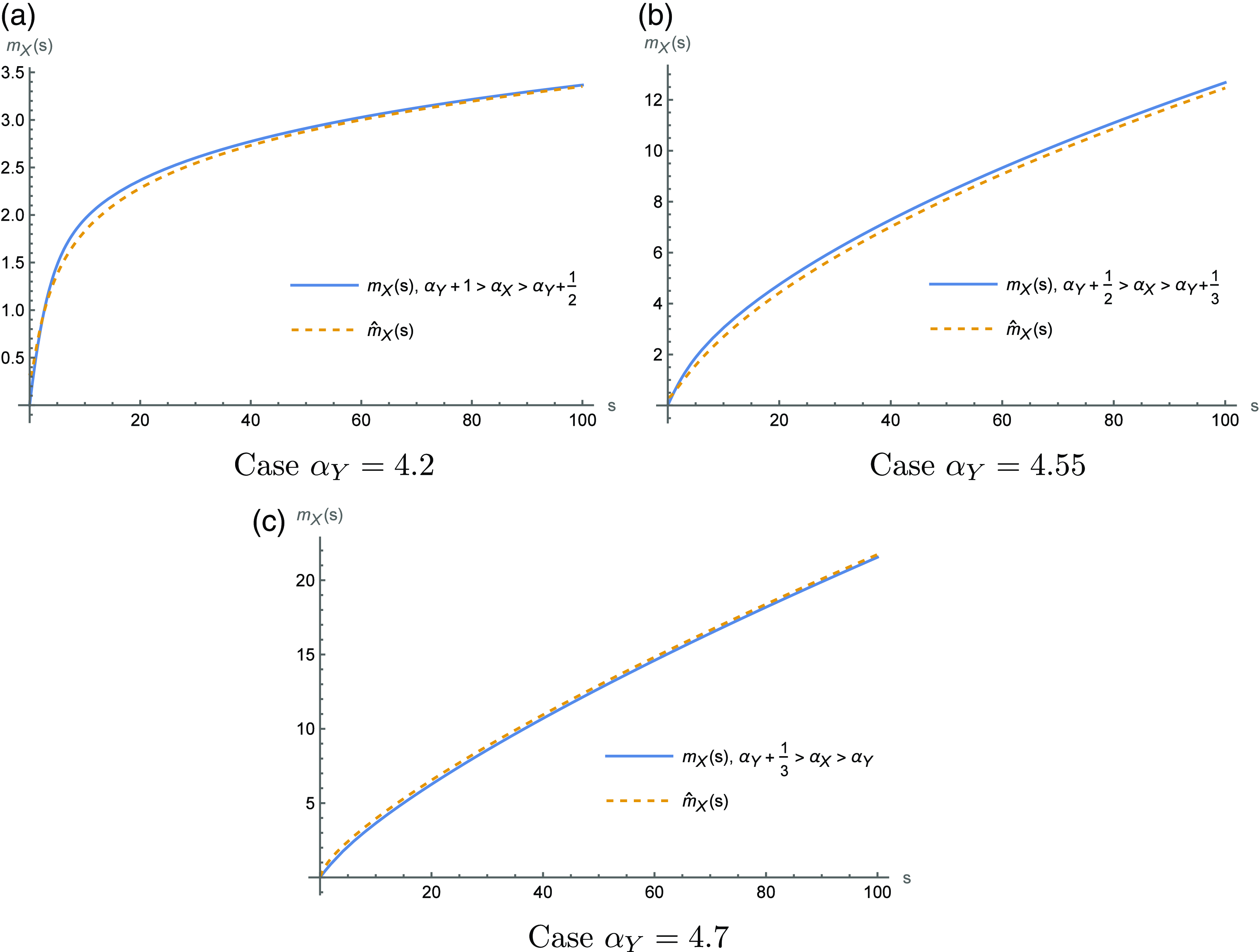
-
•
$\widehat{m}_X(s)=s\frac{f_X(s) }{f_Y(s)}\left(1+\mu_{X}\frac{f_Y(s) }{s f_X(s)}-\frac{f_X(s) }{f_Y(s)}\right)$
in cases (a) and (b). -
•
$\widehat{m}_X(s)=s\frac{f_X(s) }{f_Y(s)}\left(1-\frac{f_X(s) }{f_Y(s)}+\left(\frac{f_X(s) }{f_Y(s)}\right)^2\right)$
in case (c).


4.5. Equal indices (
$\alpha_X=\alpha_Y$
)

The following results describe the asymptotic behavior of $m_X(\!\cdot\!)$
when both variables have the same index, and under the assumption of asymptotic proportionality between the densities. Let us note that if
$m_X(\!\cdot\!)$
when both variables have the same index, and under the assumption of asymptotic proportionality between the densities. Let us note that if $X\overset{\mathrm{d}}{=} Y$
, then
$X\overset{\mathrm{d}}{=} Y$
, then $m_X(s)=m_Y(s)$
for all s in the support of S. Hence, as
$m_X(s)=m_Y(s)$
for all s in the support of S. Hence, as $m_X(s)+m_Y(s)=s$
, it is direct to see that, for equally distributed variables,
$m_X(s)+m_Y(s)=s$
, it is direct to see that, for equally distributed variables, $m_X(s)=\frac{s}{2}$
. The following result provides the asymptotic expression of
$m_X(s)=\frac{s}{2}$
. The following result provides the asymptotic expression of $m_X(\!\cdot\!)$
when both densities have the same index and are asymptotically proportional but not necessarily equal.
$m_X(\!\cdot\!)$
when both densities have the same index and are asymptotically proportional but not necessarily equal.
Proposition 4.9. Let X and Y be positive random variables possessing asymptotically smooth density functions $f_X(\!\cdot\!)$
and
$f_X(\!\cdot\!)$
and $f_Y(\!\cdot\!)$
with respective tail indices
$f_Y(\!\cdot\!)$
with respective tail indices $\alpha _{X}$
and
$\alpha _{X}$
and $\alpha _{Y}$
such that
$\alpha _{Y}$
such that $\alpha _{Y}=\alpha _{X}$
and
$\alpha _{Y}=\alpha _{X}$
and $f_{X}(s)=c f_{Y}(s)\left( 1+o\left( 1\right) \right)$
with
$f_{X}(s)=c f_{Y}(s)\left( 1+o\left( 1\right) \right)$
with $c\gt0$
. Then
$c\gt0$
. Then
 \begin{equation} m_{X}(s)=\frac{c}{1+c}s \left(1+ \frac{1}{s}\left(\frac{\alpha}{1+c}\left(\mu_Y-\mu_X\right) +\frac{\mu_X}{c}-\mu_Y\right)\left( 1+o\left( 1\right) \right) \right) \end{equation}
as s tends to infinity.
Proof. We consider $\alpha=\alpha _{Y}=\alpha _{X}$
, and we can write:
$\alpha=\alpha _{Y}=\alpha _{X}$
, and we can write:
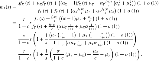 \begin{eqnarray*} m_{X}(s)&=&\frac{sf_{X}\left( s\right) +\mu _{X}f_{Y}\left( s\right)+\left( (\alpha_X -1)f_{X}\left( s\right)\mu_{Y}+\alpha_Y \frac{f_{Y}\left( s\right) }{s}\left(\sigma^2_X+\mu _{X}^2\right)\right) \left( 1+o\left( 1\right) \right)}{ f_{X}\left( s\right)+f_{Y}\left( s\right)+\left( \alpha_X \frac{f_{X}\left( s\right)}{s}\mu _{Y}+\alpha_Y \frac{f_{Y}\left( s\right) }{s}\mu _{X}\right) \left( 1+o\left( 1\right) \right)}\\ &=&\frac{c}{1+c}s \frac{f_{Y}\left( s\right) +\frac{f_{Y}\left( s\right) }{s}\left((\alpha-1)\mu _{Y} +\frac{\mu_X}{c}\right)\left( 1+o\left( 1\right) \right) }{f_{Y}\left( s\right) +\frac{f_{Y}\left( s\right) }{s}\left( \alpha\mu _{Y}\frac{c}{1+c}+\mu_X \alpha\frac{1}{1+c}\right)\left( 1+o\left( 1\right) \right) } \\ &=&\frac{c}{1+c}s \left(1+ \frac{1}{s}\frac{\left(\mu_{Y}\left(\frac{\alpha}{1+c}-1\right) +\mu_X\left(\frac{1}{c}-\frac{\alpha}{1+c}\right)\right)\left( 1+o\left( 1\right) \right) }{1 +\frac{1}{s}\left( \alpha \mu _{Y}\frac{c}{1+c}+\mu_X \alpha\frac{1}{1+c}\right)\left( 1+o\left( 1\right) \right) } \right) \\ &=&\frac{c}{1+c}s \left(1+ \frac{1}{s}\left(\frac{\alpha}{1+c}\left(\mu_Y-\mu_X\right) +\frac{\mu_X}{c}-\mu_Y\right)\left( 1+o\left( 1\right) \right) \right) .\end{eqnarray*}
This ends the proof.
If $X\overset{\mathrm{d}}{=} Y$
, since
$X\overset{\mathrm{d}}{=} Y$
, since $c=1$
and
$c=1$
and $\mu_X=\mu_Y$
, the term
$\mu_X=\mu_Y$
, the term $\frac{1}{s}\left(\frac{\alpha}{1+c}\left(\mu_Y-\mu_X\right) +\frac{\mu_X}{c}-\mu_Y\right)$
in (4.3) is zero and the expression provided in Proposition 4.9 corresponds to
$\frac{1}{s}\left(\frac{\alpha}{1+c}\left(\mu_Y-\mu_X\right) +\frac{\mu_X}{c}-\mu_Y\right)$
in (4.3) is zero and the expression provided in Proposition 4.9 corresponds to $m_X(s)=\frac{s}{2}$
as expected.
$m_X(s)=\frac{s}{2}$
as expected.
Example 4.10. Consider two independent random variables $X\sim P(IV)(\theta_X, \alpha,\vartheta,\lambda_X)$
and
$X\sim P(IV)(\theta_X, \alpha,\vartheta,\lambda_X)$
and $Y\sim P(IV)(\theta_Y,\alpha,\vartheta,\lambda_Y)$
with
$Y\sim P(IV)(\theta_Y,\alpha,\vartheta,\lambda_Y)$
with $\alpha\gt3$
. Without loss of generality, we can assume
$\alpha\gt3$
. Without loss of generality, we can assume $\vartheta=0$
. Here, the slowly varying function associated to the density
$\vartheta=0$
. Here, the slowly varying function associated to the density $f_X(\!\cdot\!)$
is given by:
$f_X(\!\cdot\!)$
is given by:
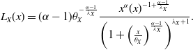 \begin{equation*} L_X(x)=(\alpha-1)\theta_X^{-\frac{\alpha-1}{\lambda_X}} \frac{x^{\alpha}(x)^{-1+\frac{\alpha-1}{\lambda_X}}}{\left(1+\left(\frac{x}{\theta_X}\right)^{\frac{\alpha-1}{\lambda_X}}\right)^{\lambda_X+1}}. \end{equation*}
Note that $\frac{f_X(s)}{f_Y(s)}=\frac{L_X(s)}{L_Y(s)}$
. Therefore, we can write
$\frac{f_X(s)}{f_Y(s)}=\frac{L_X(s)}{L_Y(s)}$
. Therefore, we can write $f_X(s)=c f_{Y}(s)\left( 1+g_{IV}\left(x\right) \right)$
, where
$f_X(s)=c f_{Y}(s)\left( 1+g_{IV}\left(x\right) \right)$
, where
 \begin{align*} g_{IV}(x)=x^{-\frac{(\alpha-1)(\lambda_X-\lambda_Y)}{\lambda_X \lambda_Y}} \theta_X^{\frac{1-\alpha}{\lambda_X}}\left(1+\left(\frac{x}{\theta_X}\right)^{\frac{\alpha-1}{\lambda_X}}\right)^{-(1+\lambda_X)}\left(\frac{\theta_X}{\theta_Y}\right)^{1-\alpha} \theta_Y^{\frac{\alpha-1}{\lambda_Y}}\left(1+\left(\frac{x}{\theta_Y}\right)^{\frac{\alpha-1}{\lambda Y}}\right)^{1+\lambda_Y}-1, \end{align*}
verifying $g_{IV}(x)=o(1)$
and
$g_{IV}(x)=o(1)$
and $c=\left(\frac{\theta_X}{\theta_Y}\right)^{\alpha-1}$
. In particular, if
$c=\left(\frac{\theta_X}{\theta_Y}\right)^{\alpha-1}$
. In particular, if $\lambda=\lambda_X=\lambda_Y$
, then
$\lambda=\lambda_X=\lambda_Y$
, then
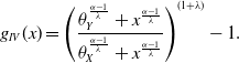 \begin{align*} g_{IV}(x)=\left(\frac{\theta_Y^{\frac{\alpha-1}{\lambda}}+x^{\frac{\alpha-1}{\lambda}}}{\theta_X^{\frac{\alpha-1}{\lambda}}+x^{\frac{\alpha-1}{\lambda}}}\right)^{(1+\lambda)}-1. \end{align*}
Let us consider two independent random variables $X\sim P(IV)(\theta_X, \alpha,\vartheta,\lambda)$
and
$X\sim P(IV)(\theta_X, \alpha,\vartheta,\lambda)$
and $Y\sim P(IV)(\theta_Y,\alpha,\vartheta,\lambda)$
such that
$Y\sim P(IV)(\theta_Y,\alpha,\vartheta,\lambda)$
such that $\alpha=7$
,
$\alpha=7$
, $\theta_X=1$
,
$\theta_X=1$
, $\theta_Y=2$
,
$\theta_Y=2$
, $\lambda=2$
and
$\lambda=2$
and $\vartheta=0$
. Figure 11 shows the same asymptotic behavior of
$\vartheta=0$
. Figure 11 shows the same asymptotic behavior of $m_X(\!\cdot\!)$
and
$m_X(\!\cdot\!)$
and
 \begin{align*}\widehat{m}_X(s)=\frac{c}{1+c}s \left(1+ \frac{1}{s}\left(\frac{\alpha}{1+c}\left(\mu_Y-\mu_X\right) +\frac{\mu_X}{c}-\mu_Y\right) \right), \; \; c=\frac{1}{64}.\end{align*}
Conditional expectation $m_X(\!\cdot\!)$
when
$m_X(\!\cdot\!)$
when $X\sim P(IV)(\theta_X, \alpha,\vartheta,\lambda)$
and
$X\sim P(IV)(\theta_X, \alpha,\vartheta,\lambda)$
and $Y\sim P(IV)(\theta_Y,\alpha,\vartheta,\lambda)$
with
$Y\sim P(IV)(\theta_Y,\alpha,\vartheta,\lambda)$
with $\alpha=7$
,
$\alpha=7$
, $\theta_X=1$
,
$\theta_X=1$
, $\theta_Y=2$
,
$\theta_Y=2$
, $\lambda=2$
and
$\lambda=2$
and $\vartheta=0$
.
$\vartheta=0$
.
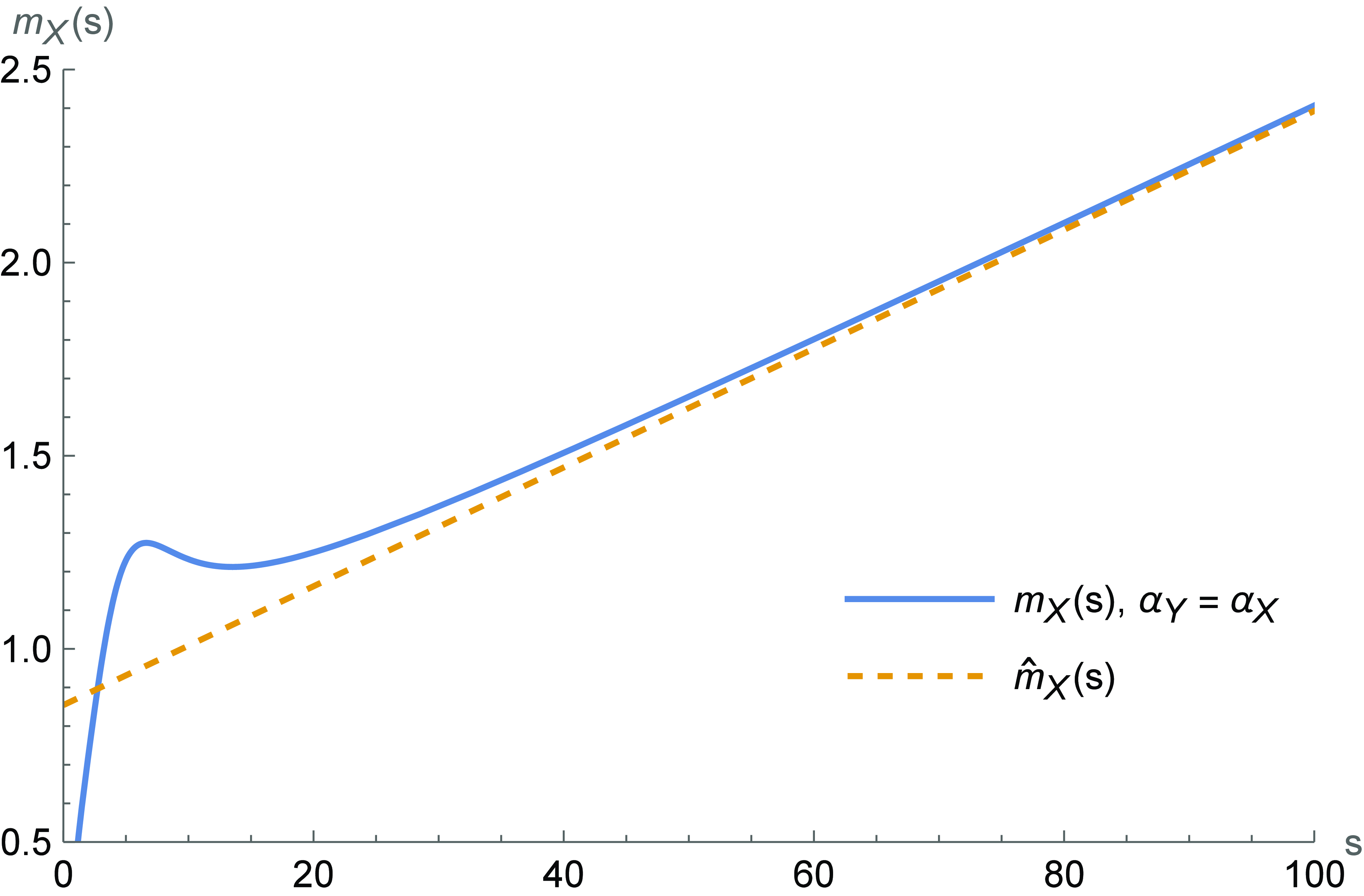
From Proposition 4.9, when the densities have equal tail indices and they are asymptotically proportional, $m_X\left(\cdot\right)$
can be approximated by a function where the term which dominates is
$m_X\left(\cdot\right)$
can be approximated by a function where the term which dominates is $\frac{c}{1+c}s$
. However, from Proposition 4.7, if
$\frac{c}{1+c}s$
. However, from Proposition 4.7, if $1\gt\alpha_X-\alpha_Y\gt0$
, the asymptotic behavior of
$1\gt\alpha_X-\alpha_Y\gt0$
, the asymptotic behavior of $m_X\left(\cdot\right)$
can be approximated by a function where the dominant term is
$m_X\left(\cdot\right)$
can be approximated by a function where the dominant term is $s^{\alpha_Y+1-\alpha_X}\frac{L_{X}\left( s\right) }{L_{Y}\left(s\right)}$
, with
$s^{\alpha_Y+1-\alpha_X}\frac{L_{X}\left( s\right) }{L_{Y}\left(s\right)}$
, with $1\gt\alpha_Y+1-\alpha_{X}\gt0$
. Hence, if
$1\gt\alpha_Y+1-\alpha_{X}\gt0$
. Hence, if $0 \lt \alpha_X-\alpha_Y \lt 1$
, asymptotically,
$0 \lt \alpha_X-\alpha_Y \lt 1$
, asymptotically, $m_X\left(\cdot\right)$
increases faster than it does if the indices are equal. And, the nearer the indices, the faster that
$m_X\left(\cdot\right)$
increases faster than it does if the indices are equal. And, the nearer the indices, the faster that $m_X\left(\cdot\right)$
asymptotically increases.
$m_X\left(\cdot\right)$
asymptotically increases.
5. Extensions to zero-augmented random variables
Zero-augmented distributions combine a continuous distribution on the positive real line and a point probability mass at zero. For instance, in the context of risk-sharing schemes, zero-augmented distributions are often encountered since the probability mass at zero corresponds to participants who do not file any claim against the scheme.
In this section, we show that, adding a probability mass at 0 to a distribution with regularly varying density, tail indices still play a role in the limit behavior of the conditional mean given the sum. The next result extends Propositions 4.1 and 4.2 to the zero-augmented case.
Proposition 5.1. Let X and Y be nonnegative random variables such that $X=I_{X}C_{X}$
and
$X=I_{X}C_{X}$
and $Y=I_{Y}C_{Y}$
where
$Y=I_{Y}C_{Y}$
where $I_{X}$
,
$I_{X}$
, $C_{X}$
,
$C_{X}$
, $I_{Y}$
, and
$I_{Y}$
, and $C_{Y}$
are independent,
$C_{Y}$
are independent, $I_{X}$
and
$I_{X}$
and $I_{Y}$
are Bernoulli distributed with mean
$I_{Y}$
are Bernoulli distributed with mean $p_{X}$
and
$p_{X}$
and $p_{Y}$
,
$p_{Y}$
, $0 \lt p_{X},p_{Y}\leq 1$
, and
$0 \lt p_{X},p_{Y}\leq 1$
, and $C_{X}$
and
$C_{X}$
and $C_{Y}$
possess asymptotically smooth density functions
$C_{Y}$
possess asymptotically smooth density functions $f_{C_X}(\!\cdot\!)$
and
$f_{C_X}(\!\cdot\!)$
and $f_{C_Y}(\!\cdot\!)$
with tail indices
$f_{C_Y}(\!\cdot\!)$
with tail indices $\alpha _{C_X}$
and
$\alpha _{C_X}$
and $\alpha _{C_Y}$
such that
$\alpha _{C_Y}$
such that $\min\{\alpha _{C_X},\alpha _{C_Y}\}\gt2$
. Then, as s tends to infinity,
$\min\{\alpha _{C_X},\alpha _{C_Y}\}\gt2$
. Then, as s tends to infinity,
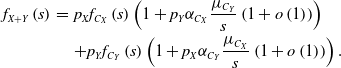 \begin{eqnarray*} f_{X+Y}\left( s\right) &=&p_Xf_{C_X}\left( s\right) \left( 1+p_Y\alpha _{C_X}\frac{\mu _{C_Y}}{s}\left( 1+o\left( 1\right) \right) \right)\\ &&+p_Yf_{C_Y}\left( s\right) \left( 1+p_X\alpha _{C_Y}\frac{\mu _{C_X} }{s} \left( 1+o\left( 1\right) \right) \right) .\end{eqnarray*}
In addition, if $\min\{\alpha _{C_X},\alpha _{C_Y}\}\gt3$
,
$\min\{\alpha _{C_X},\alpha _{C_Y}\}\gt3$
, $\mu_{\widetilde{C}_X},\mu_{\widetilde{C}_Y}$
are finite and the conditional mean given the sum satisfies that, as s tends to
$\mu_{\widetilde{C}_X},\mu_{\widetilde{C}_Y}$
are finite and the conditional mean given the sum satisfies that, as s tends to $\infty$
,
$\infty$
,
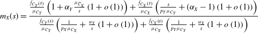 \begin{equation} m_{X}(s)=\frac{\frac{f_{C_Y}\left( s\right) }{\mu_{C_Y}}\left( 1+\alpha _{Y}\frac{\mu_{\widetilde{C}_X}}{s}\left( 1+o\left( 1\right) \right) \right)+\frac{f_{C_X}\left( s\right)}{\mu_{C_X}} \left( \frac{s}{p_Y \mu_{C_Y}}+(\alpha _{X}-1)\left( 1+o\left( 1\right) \right) \right) }{\frac{f_{C_Y}\left( s\right)}{\mu_{C_Y}} \left( \frac{1}{p_X \mu_{C_X}}+\frac{\alpha _{Y}}{s}\left( 1+o\left( 1\right)\right)\right) +\frac{f_{C_X}\left( s\right) }{\mu_{C_X}}\left(\frac{1}{p_Y \mu_{C_Y}}+\frac{\alpha _{X}}{s}\left( 1+o\left( 1\right) \right) \right)}\end{equation}
Proof. As the sum of two random variables obeying zero-augmented distributions, $X+Y$
also obeys a zero-augmented distribution with probability mass
$X+Y$
also obeys a zero-augmented distribution with probability mass $(1-p_X)(1-p_Y)$
at 0. For
$(1-p_X)(1-p_Y)$
at 0. For $s\gt0$
, the density function of
$s\gt0$
, the density function of $X+Y$
can be written as
$X+Y$
can be written as
 \begin{equation*}f_{X+Y}\left( s\right) =p_X(1-p_Y)f_{C_X}\left(s\right)+(1-p_X)p_Yf_{C_Y}\left(s\right)+p_Xp_Yf_{C_X+C_Y}\left(s\right).\end{equation*}
Now, Proposition 4.1 applies to $f_{C_X+C_Y}(\!\cdot\!)$
so that
$f_{C_X+C_Y}(\!\cdot\!)$
so that
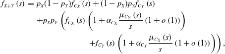 \begin{eqnarray*}f_{X+Y}\left( s\right) &=&p_X(1-p_Y)f_{C_X}\left(s\right)+(1-p_X)p_Yf_{C_Y}\left(s\right)\\&&+p_Xp_Y\left(f_{C_X}\left( s\right) \left( 1+\alpha _{C_X}\frac{\mu_{C_Y}\left( s\right) }{s}\left( 1+o\left( 1\right) \right) \right)\right.\\&&\left.\hspace{22mm}+f_{C_Y}\left( s\right) \left( 1+\alpha _{C_Y}\frac{\mu _{C_X}\left( s\right) }{s}\left( 1+o\left( 1\right) \right) \right)\right),\end{eqnarray*}
which ends the first part of the proof.
In order to obtain the expression of the conditional mean, it is known from Proposition 2.2(iii) in Denuit (Reference Denuit2019) that
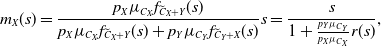 \begin{equation} m_{X}(s) =\frac{p_{X}\mu _{C_X}f_{\widetilde{C}_{X}+Y}(s)}{p_{X}\mu _{C_X}f_{\widetilde{C}_{X}+Y}(s)+p_{Y}\mu _{C_Y}f_{\widetilde{C}_{Y}+X}(s)}s=\frac{s}{1+\frac{p_{Y}\mu _{C_Y}}{p_{X}\mu _{C_X}}r(s)},\end{equation}
with $r(s)=\frac{f_{\widetilde{C}_{Y}+X}(s)}{f_{\widetilde{C}_{X}+Y}(s)}$
. Analogously as above,
$r(s)=\frac{f_{\widetilde{C}_{Y}+X}(s)}{f_{\widetilde{C}_{X}+Y}(s)}$
. Analogously as above, $\widetilde{C}_{Y}+X$
is a mixture of
$\widetilde{C}_{Y}+X$
is a mixture of $\widetilde{C}_{Y}$
(with probability
$\widetilde{C}_{Y}$
(with probability $1-p_X$
) and
$1-p_X$
) and $\widetilde{C}_{Y}+C_X$
(with probability
$\widetilde{C}_{Y}+C_X$
(with probability $p_X$
). A similar representation holds for
$p_X$
). A similar representation holds for $\widetilde{C}_{X}+Y$
. Therefore, we can write:
$\widetilde{C}_{X}+Y$
. Therefore, we can write:
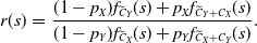 \begin{eqnarray*} r(s)&=&\frac{(1-p_X)f_{\widetilde{C}_{Y}}(s)+p_X f_{\widetilde{C}_{Y}+C_X}(s)}{(1-p_Y)f_{\widetilde{C}_{X}}(s)+p_Y f_{\widetilde{C}_{X}+C_Y}(s)}.\end{eqnarray*}
Since $\widetilde{C}_{Y},\widetilde{C}_{X},C_Y$
, and
$\widetilde{C}_{Y},\widetilde{C}_{X},C_Y$
, and $C_X$
are positive random variables with
$C_X$
are positive random variables with $\alpha_{\widetilde{C}_{Z}}=\alpha_{C_{Z}}-1$
for
$\alpha_{\widetilde{C}_{Z}}=\alpha_{C_{Z}}-1$
for $Z=X,Y$
, using the asymptotic expansion provided in Proposition 4.1, we can obtain
$Z=X,Y$
, using the asymptotic expansion provided in Proposition 4.1, we can obtain
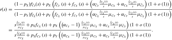 \begin{eqnarray*} r(s)&=&\frac{(1-p_X)f_{\widetilde{C}_{Y}}(s)+p_X \left(f_{\widetilde{C}_{Y}}\left( s\right)+f_{C_X}\left( s\right)+\left(\alpha_{\widetilde{C}_{Y}} \frac{f_{\widetilde{C}_{Y}}\left( s\right)}{s}\mu _{C_X}+\alpha_{C_X} \frac{f_{C_X}\left( s\right) }{s}\mu _{\widetilde{C}_{Y}}\right) \left( 1+o\left( 1\right) \right)\right)}{(1-p_Y)f_{\widetilde{C}_{X}}(s)+p_Y \left(f_{\widetilde{C}_{X}}\left( s\right)+f_{C_Y}\left( s\right)+\left( \alpha_{\widetilde{C}_{X}} \frac{f_{\widetilde{C}_{X}}\left( s\right)}{s}\mu _{C_Y}+\alpha_{C_Y} \frac{f_{C_Y}\left( s\right) }{s}\mu _{\widetilde{C}_{X}}\right) \left( 1+o\left( 1\right) \right)\right)}\\ &=&\frac{s \frac{f_{C_Y}\left( s\right)}{\mu_{C_Y}}+p_X f_{C_X}\left( s\right)+p_X\left( \left(\alpha_{C_{Y}}-1\right) \frac{f_{C_Y}\left( s\right)}{\mu_{C_Y}}\mu _{C_X}+\alpha_{C_X} \frac{f_{C_X}\left( s\right) }{s}\mu _{\widetilde{C}_{Y}}\right) \left( 1+o\left( 1\right) \right)}{s\frac{ f_{C_X}\left( s\right)}{\mu_{C_X}}+p_Y f_{C_Y}\left( s\right)+p_Y\left( \left(\alpha_{C_{X}}-1\right) \frac{f_{C_X}\left( s\right)}{\mu_{C_X}}\mu _{C_Y}+\alpha_{C_Y} \frac{f_{C_Y}\left( s\right) }{s}\mu _{\widetilde{C}_{X}}\right) \left( 1+o\left( 1\right) \right)}.\end{eqnarray*}
Hence, from (5.2), and noticing that $\frac{\mu_{\widetilde{C}_Y}}{s}=o\left(1\right)$
,
$\frac{\mu_{\widetilde{C}_Y}}{s}=o\left(1\right)$
,
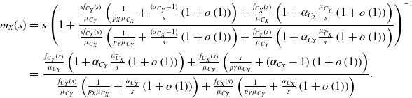 \begin{eqnarray*} m_{X}(s)&=&s\left(1+\frac{\frac{s f_{C_Y}\left( s\right)}{\mu_{C_Y}} \left( \frac{1}{p_X \mu_{C_X}}+\frac{(\alpha _{C_Y}-1)}{s}\left( 1+o\left( 1\right) \right) \right) +\frac{f_{C_X}\left( s\right) }{\mu_{C_X}}\left( 1+\alpha _{C_X}\frac{\mu_{\widetilde{C}_Y}}{s}\left( 1+o\left( 1\right) \right) \right)}{\frac{s f_{C_X}\left( s\right)}{\mu_{C_X}} \left( \frac{1}{p_Y \mu_{C_Y}}+\frac{(\alpha _{C_X}-1)}{s}\left( 1+o\left( 1\right) \right) \right) +\frac{f_{C_Y}\left( s\right) }{\mu_{C_Y}}\left( 1+\alpha _{C_Y}\frac{\mu_{\widetilde{C}_X}}{s}\left( 1+o\left( 1\right) \right) \right)}\right)^{-1}\\ &=&\frac{\frac{f_{C_Y}\left( s\right) }{\mu_{C_Y}}\left( 1+\alpha _{C_Y}\frac{\mu_{\widetilde{C}_X}}{s}\left( 1+o\left( 1\right) \right) \right)+\frac{f_{C_X}\left( s\right)}{\mu_{C_X}} \left(\frac{s}{p_Y \mu_{C_Y}}+(\alpha _{C_X}-1)\left( 1+o\left( 1\right) \right) \right) }{\frac{f_{C_Y}\left( s\right)}{\mu_{C_Y}} \left( \frac{1}{p_X \mu_{C_X}}+\frac{\alpha _{C_Y}}{s}\left( 1+o\left( 1\right)\right)\right) +\frac{f_{C_X}\left( s\right) }{\mu_{C_X}}\left(\frac{1}{p_Y \mu_{C_Y}}+\frac{\alpha _{C_X}}{s}\left( 1+o\left( 1\right) \right) \right)}.\end{eqnarray*}
This ends the proof.
When $p_X=p_Y=1$
, Proposition 5.1 reduces to Propositions 4.1 and 4.2, as expected. Similarly as in Section 3, we can derive the asymptotic level of
$p_X=p_Y=1$
, Proposition 5.1 reduces to Propositions 4.1 and 4.2, as expected. Similarly as in Section 3, we can derive the asymptotic level of $m_X(\!\cdot\!)$
when we consider zero-augmented random variables. Let us remark that, in order to obtain the asymptotic expression of
$m_X(\!\cdot\!)$
when we consider zero-augmented random variables. Let us remark that, in order to obtain the asymptotic expression of $m_X(\!\cdot\!)$
, contrary to the case of continuous random variables, where it is required that
$m_X(\!\cdot\!)$
, contrary to the case of continuous random variables, where it is required that $\alpha_X\gt3$
and
$\alpha_X\gt3$
and $\alpha_Y\gt2$
, when considering zero-augmented random variables the hypothesis
$\alpha_Y\gt2$
, when considering zero-augmented random variables the hypothesis $\min\{\alpha _{C_X},\alpha _{C_Y}\}\gt3$
is included. This assumption is required because, by Denuit (Reference Denuit2019), for zero-augmented distributions, we use the expression
$\min\{\alpha _{C_X},\alpha _{C_Y}\}\gt3$
is included. This assumption is required because, by Denuit (Reference Denuit2019), for zero-augmented distributions, we use the expression $m_{X}(s) =\frac{p_{X}\mu _{C_X}f_{\widetilde{C}_{X}+Y}(s)}{p_{X}\mu _{C_X}f_{\widetilde{C}_{X}+Y}(s)+p_{Y}\mu _{C_Y}f_{\widetilde{C}_{Y}+X}(s)}s,$
instead of the expression
$m_{X}(s) =\frac{p_{X}\mu _{C_X}f_{\widetilde{C}_{X}+Y}(s)}{p_{X}\mu _{C_X}f_{\widetilde{C}_{X}+Y}(s)+p_{Y}\mu _{C_Y}f_{\widetilde{C}_{Y}+X}(s)}s,$
instead of the expression $m_{X}(s) =\mu _{X}\frac{f_{\widetilde{X}+Y}(s)}{f_{X+Y}(s)}$
for continuous variables. Hence, the expectations of both size-biased transformations of
$m_{X}(s) =\mu _{X}\frac{f_{\widetilde{X}+Y}(s)}{f_{X+Y}(s)}$
for continuous variables. Hence, the expectations of both size-biased transformations of $C_X$
and
$C_X$
and $C_Y$
are required to be finite.
$C_Y$
are required to be finite.
Corollary 5.2. Let X and Y be nonnegative random variables such that $X=I_{X}C_{X}$
and
$X=I_{X}C_{X}$
and $Y=I_{Y}C_{Y}$
where
$Y=I_{Y}C_{Y}$
where $I_{X}$
,
$I_{X}$
, $C_{X}$
,
$C_{X}$
, $I_{Y}$
, and
$I_{Y}$
, and $C_{Y}$
are independent,
$C_{Y}$
are independent, $I_{X}$
and
$I_{X}$
and $I_{Y}$
are Bernoulli distributed with mean
$I_{Y}$
are Bernoulli distributed with mean $p_{X}$
and
$p_{X}$
and $p_{Y}$
,
$p_{Y}$
, $0 \lt p_{X},p_{Y}\leq 1$
, and
$0 \lt p_{X},p_{Y}\leq 1$
, and $C_{X}$
and
$C_{X}$
and $C_{Y}$
possess asymptotically smooth density functions
$C_{Y}$
possess asymptotically smooth density functions $f_{C_X}(\!\cdot\!)$
and
$f_{C_X}(\!\cdot\!)$
and $f_{C_Y}(\!\cdot\!)$
with tail indices
$f_{C_Y}(\!\cdot\!)$
with tail indices $\alpha _{C_X}$
and
$\alpha _{C_X}$
and $\alpha _{C_Y}$
such that
$\alpha _{C_Y}$
such that $\min\{\alpha _{C_X},\alpha _{C_Y}\}\gt3$
and respective associated slowly varying functions
$\min\{\alpha _{C_X},\alpha _{C_Y}\}\gt3$
and respective associated slowly varying functions $L_{C_X}$
and
$L_{C_X}$
and $L_{C_Y}$
.
$L_{C_Y}$
.
-
• If
$\alpha_{C_X}\gt\alpha_{C_Y}+1$
, then
$\lim_{s \rightarrow \infty}m_{X}(s)=\mathrm{E}[X]$
, -
• If
$\alpha_{C_Y}+1\gt\alpha_{C_X}\geq \alpha_{C_Y}$
, then
$m_{X}(s)\rightarrow \infty$
as
$s\rightarrow \infty$
. -
• If
$\alpha_{C_X}=\alpha_{C_Y}+1$
:-
- If
$ \frac{L_{C_X}(s)}{L_{C_Y}(s)}\rightarrow\infty$
as
$s\rightarrow \infty$
, then
$m_{X}(s)\rightarrow \infty$
as
$s\rightarrow \infty$
. -
- If
$\lim_{s\rightarrow \infty }\frac{L_{C_X}(s)}{L_{C_Y}(s)}=k$
with
$k \geq 0$
, then
$\lim_{s\rightarrow \infty }m_{X}(s)=\mathrm{E}[X]+\frac{p_X}{p_Y}k$
.
-


Proof. Let us note that expression 5.1 can be rewritten as
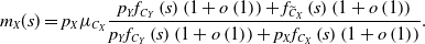 \begin{equation*} m_{X}(s)=p_X\mu_{C_X}\frac{p_Y f_{C_Y}\left( s\right) \left(1+o\left(1\right)\right)+f_{\widetilde{C}_X}\left( s\right) \left(1+o\left(1\right)\right)}{p_Yf_{C_Y}\left( s\right)\left( 1+o\left( 1\right)\right) +p_Xf_{C_X}\left( s\right)\left( 1+o\left( 1\right)\right)}.\end{equation*}
And, therefore, as $s\rightarrow \infty$
.
$s\rightarrow \infty$
.
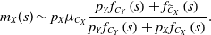 \begin{equation}m_{X}(s) \sim p_X\mu_{C_X}\frac{p_Y f_{C_Y}\left( s\right)+f_{\widetilde{C}_X}\left( s\right) }{p_Yf_{C_Y}\left( s\right) +p_Xf_{C_X}\left( s\right)}.\end{equation}
As $f_{C_X}(\!\cdot\!)$
and
$f_{C_X}(\!\cdot\!)$
and $f_{C_Y}(\!\cdot\!)$
are asymptotically smooth densities with respective indices
$f_{C_Y}(\!\cdot\!)$
are asymptotically smooth densities with respective indices $\alpha _{C_X},\alpha _{C_Y}\gt2$
, then:
$\alpha _{C_X},\alpha _{C_Y}\gt2$
, then:
-
• If
$\alpha_{C_X}\gt\alpha_{C_Y}+1$
, then
$f_{C_X}\left( s\right) =o\left( f_{C_Y}\left( s\right) \right) $
,
$f_{\widetilde{C}_X}\left( s\right) =o\left(f_{C_Y}\left( s\right) \right) $
. Since
$\mathrm{E}[X]=p_X\mu_{C_X}$
, from (5.3),
$\lim_{s \rightarrow \infty}m_{X}(s)=\mathrm{E}[X]$
. -
• If
$\alpha_{C_Y}+1\gt\alpha_{C_X}\geq \alpha_{C_Y}$
, then
$f_{C_Y}\left( s\right) =o\left(f_{\widetilde{C}_X}\left( s\right) \right) $
and
$f_{C_X}\left( s\right) =o\left( f_{\widetilde{C}_X}\left( s\right) \right)$
. From (5.3), it is direct that
$m_{X}(s)\rightarrow \infty$
as
$s\rightarrow \infty$
. -
• If
$\alpha_{C_X}=\alpha_{C_Y}+1$
, then
$f_{C_X}\left( s\right) =o\left( f_{C_Y}\left( s\right) \right) $
and we can rewrite (5.3) as, if
$s \rightarrow \infty$
, by By replacing the limit behavior of
\begin{equation*} m_{X}(s) \sim p_X\frac{\mu_{C_X} p_Y L_{C_Y}\left( s\right)+L_{C_X}\left( s\right) }{p_YL_{C_Y}\left( s\right) +o\left(L_{C_Y}\left( s\right)\right)}.\end{equation*}
$\frac{L_{C_X}(s)}{L_{C_Y}(s)}$
, the assertion follows.


This ends the proof.
As expected, considering $p_X=p_Y=1$
, Corollary 5.2 reduces to the asymptotic levels provided in Section 3. Note that, similarly to the continuous case, we can obtain the asymptotic expansion of the conditional mean given the sum considering zero-augmented random variables. However, in order to provide simpler expressions for the zero augmented case, distinctly as in some cases considered in the continuous framework, here we provide expansions considering two significant terms. Therefore, the case
$p_X=p_Y=1$
, Corollary 5.2 reduces to the asymptotic levels provided in Section 3. Note that, similarly to the continuous case, we can obtain the asymptotic expansion of the conditional mean given the sum considering zero-augmented random variables. However, in order to provide simpler expressions for the zero augmented case, distinctly as in some cases considered in the continuous framework, here we provide expansions considering two significant terms. Therefore, the case $\alpha _{Y}+1\gt\alpha _{X}\gt\alpha_{Y}$
is divided into two “sub-cases” instead of three as it was considered in Proposition 4.7. Let us note that if
$\alpha _{Y}+1\gt\alpha _{X}\gt\alpha_{Y}$
is divided into two “sub-cases” instead of three as it was considered in Proposition 4.7. Let us note that if $p_X=p_Y=1$
, the asymptotic expressions (except the one mentioned) are the expansions provided in Section 4, as expected.
$p_X=p_Y=1$
, the asymptotic expressions (except the one mentioned) are the expansions provided in Section 4, as expected.
Corollary 5.3. Let X and Y be nonnegative random variables such that $X=I_{X}C_{X}$
and
$X=I_{X}C_{X}$
and $Y=I_{Y}C_{Y}$
where
$Y=I_{Y}C_{Y}$
where $I_{X}$
,
$I_{X}$
, $C_{X}$
,
$C_{X}$
, $I_{Y}$
, and
$I_{Y}$
, and $C_{Y}$
are independent,
$C_{Y}$
are independent, $I_{X}$
and
$I_{X}$
and $I_{Y}$
are Bernoulli distributed with mean
$I_{Y}$
are Bernoulli distributed with mean $p_{X}$
and
$p_{X}$
and $p_{Y}$
,
$p_{Y}$
, $0 \lt p_{X},p_{Y}\leq 1$
, and
$0 \lt p_{X},p_{Y}\leq 1$
, and $C_{X}$
and
$C_{X}$
and $C_{Y}$
possess asymptotically smooth density functions
$C_{Y}$
possess asymptotically smooth density functions $f_{C_X}(\!\cdot\!)$
and
$f_{C_X}(\!\cdot\!)$
and $f_{C_Y}(\!\cdot\!)$
with tail indices
$f_{C_Y}(\!\cdot\!)$
with tail indices $\alpha _{C_X}$
and
$\alpha _{C_X}$
and $\alpha _{C_Y}$
such that
$\alpha _{C_Y}$
such that $\min\{\alpha _{C_X},\alpha _{C_Y}\}\gt3$
.
$\min\{\alpha _{C_X},\alpha _{C_Y}\}\gt3$
.
-
1. If
$\alpha _{C_X}\gt\alpha _{C_Y}+2$
, then, as s tends to infinity,
\begin{equation*} m_{X}(s)=p_X\mu _{C_X}+\alpha _{C_Y}\frac{p_X}{s}\sigma^2_{C_X} \left( 1+o\left( 1\right)\right). \end{equation*}
-
2. If
$\alpha _{C_Y}+2\gt \alpha_{C_X}\gt\alpha _{C_Y}+1$
, then, as s tends to infinity,
\begin{equation*} m_{X}(s)=p_X \mu_{C_X}+s\frac{p_X}{p_Y}\frac{f_{C_X}\left( s\right)}{f_{C_Y}\left( s\right)} \left( 1+o\left( 1\right) \right).\end{equation*}
-
3. If
$\alpha _{C_Y}+1\gt\alpha _{C_X}\gt\alpha _{C_Y}+\frac{1}{2}$
, then, as s tends to infinity,
\begin{equation*} m_{X}(s)=s\;\frac{f_{C_X}(s) }{f_{C_Y}(s)}\left(\frac{p_X}{p_Y}+\frac{p_X\mu_{C_X} f_{C_Y}\left( s\right)}{s f_{C_X}\left( s\right)}\left( 1+o\left( 1\right) \right)\right). \end{equation*}
-
4. If
$\alpha _{C_Y}+1\gt\alpha _{C_X}\gt\alpha_{C_Y}+\frac{1}{2}$
, then, as s tends to infinity,
\begin{equation*} m_{X}(s)=s\;\frac{p_X}{p_Y}\;\frac{f_{C_X}(s) }{f_{C_Y}(s)}\left(1-\frac{p_X}{p_Y}\frac{f_{C_X}\left( s\right)}{ f_{C_Y}\left( s\right)}\left( 1+o\left( 1\right) \right)\right).\end{equation*}
-
5. If
$\alpha _{C_Y}=\alpha _{C_X}$
and
$f_{C_X}(s)=c f_{C_Y}(s)\left( 1+o\left( 1\right) \right)$
with
$c\gt0$
, then as s tends to infinity,
\begin{equation*} m_{X}(s)= \frac{c}{\frac{p_Y}{p_X}+c}s\left(1+\frac{1}{s}\left(\frac{\mu_{C_X}p_Y}{c}-p_Y \mu_{C_Y}+\alpha\frac{p_Y}{\frac{p_Y}{p_X}+c} \left(\frac{p_Y}{p_X} \mu_{C_Y}-\mu_{C_X}\right) \right)\left( 1+o\left( 1\right)\right)\right).\end{equation*}


The proof of the Corollary is provided in Appendix C.
In addition to zero-augmented distributions, note that the findings derived in this paper can also be extended to the case of considering more than two random variables. This is a more realistic scenario for a risk-sharing pool, and the extension to this framework is provided in Appendix D. Within a larger pool with risks having regularly varying densities, if two tail indices differ in more than one unit, a sabotage scenario exists and the contribution of the risk holder with a greater index converges to the unconditional expectation as in the bivariate scenario.
Even if the results of this paper assume that the random variables are independent, an extension to an dependence setting where the dependence structure follows a Farlie–Gumbel–Morgenstern (FGM) copula can be derived, and it is considered in Appendix 11. Under this setting, a difference of more than one unit between the tail indices also leads to a sabotage scenario and the contribution of the risk holder with a greater index converges again to a constant, which, however, is different from the one obtained in the case of independence.
6. Conclusion
The monotonicity of the conditional expectations of variables given their sum is known to be relevant in several contexts. For instance, it is of great utility for actuarial applications, as the conditional expectations of variables given their sum correspond to the conditional mean risk-sharing rule and its monotonicity is referred to as the no-sabotage condition. It is also relevant in risk management, both for portfolio diagnosis and as a useful simplification to determine the natural allocation principle.
To ensure the monotonicity of $m_{X}(s)=\mathrm{E}[X|X+Y=s]$
, it is common to assume log-concave densities, meaning that variables are supposed to be light tailed, an assumption which might be too strong. In this paper, we studied the behavior of
$m_{X}(s)=\mathrm{E}[X|X+Y=s]$
, it is common to assume log-concave densities, meaning that variables are supposed to be light tailed, an assumption which might be too strong. In this paper, we studied the behavior of $m_{X}(\!\cdot\!)$
when variables are heavy tailed. In particular, we studied the behavior of the conditional expectation given the sum considering variables with regularly varying densities. We showed that, under the independence assumption, (i) a difference higher than one on the respective tail indices of X and Y implies that
$m_{X}(\!\cdot\!)$
when variables are heavy tailed. In particular, we studied the behavior of the conditional expectation given the sum considering variables with regularly varying densities. We showed that, under the independence assumption, (i) a difference higher than one on the respective tail indices of X and Y implies that $m_X(\!\cdot\!)$
cannot be monotonic over its domain, converging to the unconditional expected value and (ii) if the difference is smaller than 1,
$m_X(\!\cdot\!)$
cannot be monotonic over its domain, converging to the unconditional expected value and (ii) if the difference is smaller than 1, $m_X(\!\cdot\!)$
is not bounded as the value of the sum diverges. These implications still hold when considering independent zero-augmented random variables, as seen in Section 5, or when variables are not independent but their dependence structure follows a Farlie–Gumbel–Morgenstern copula, as seen in Appendix E. However, under this dependence structure, when indices differ in more than one unit,
$m_X(\!\cdot\!)$
is not bounded as the value of the sum diverges. These implications still hold when considering independent zero-augmented random variables, as seen in Section 5, or when variables are not independent but their dependence structure follows a Farlie–Gumbel–Morgenstern copula, as seen in Appendix E. However, under this dependence structure, when indices differ in more than one unit, $m_X(\!\cdot\!)$
does not converge to the unconditional expected value but to a different constant provided in Proposition E.1(b). In addition, implication (i) also holds in larger pools with independent risks as long as there exist two variables with a difference higher than one on the respective tail indices.
$m_X(\!\cdot\!)$
does not converge to the unconditional expected value but to a different constant provided in Proposition E.1(b). In addition, implication (i) also holds in larger pools with independent risks as long as there exist two variables with a difference higher than one on the respective tail indices.
Considering a risk-sharing scheme scenario, the result implies that, if the risks associated with the pool members have tail indices differing by more than one unit, with the conditional mean risk sharing rule there will always exist a sabotage scenario. Hence, a direct implication of this paper is that it enables practitioners to identify a necessary condition when forming a pool, based on risks having a similar tail behavior. The rule is simple: when forming a risk-sharing pool, there cannot exist tail indices of two losses’ distributions differing in more than one unit. Analogously, if the difference among all tail indices is less than one, even if we cannot state that the contribution of each participant is increasing in the total loss, we know that they are asymptotically increasing. This means that the risk-sharing will not lead to extreme cases of sabotage. Concerning risk management, an implication of the results is to provide theoretical support and formalization of the intuitions and ideas described in Major and Mildenhall (Reference Major and Mildenhall2020) and Mildenhall and Major (Reference Mildenhall and Major2022) with respect to the monotonicity of the conditional expectations for heavy-tailed distributions. It is of particular interest to see the cases described in Chapter 15.4.1. of Mildenhall and Major (Reference Mildenhall and Major2022) considering a price allocation framework for different lines of business. The connection between the difference between the tail-heaviness of the lines and the behavior of the conditional expectations provides illustrative examples of the results described in the present paper.
Under the assumption that random variables involved have finite second moments, we have also provided the asymptotic expression of $m_X(\!\cdot\!)$
. This allowed us to study its asymptotic behavior depending on the differences between the tail indices. These results have been extended to zero-augmented distributions. In this case, the difference between the tail indices of the continuous components determines the limit behavior of
$m_X(\!\cdot\!)$
. This allowed us to study its asymptotic behavior depending on the differences between the tail indices. These results have been extended to zero-augmented distributions. In this case, the difference between the tail indices of the continuous components determines the limit behavior of $m_X(\!\cdot\!)$
. An extension to several terms has also been proposed, to study the presence of sabotage opportunities within pools gathering more than two participants. Throughout the paper, several numerical examples with parametric families are provided in order to illustrate the results.
$m_X(\!\cdot\!)$
. An extension to several terms has also been proposed, to study the presence of sabotage opportunities within pools gathering more than two participants. Throughout the paper, several numerical examples with parametric families are provided in order to illustrate the results.
The analysis conducted in this paper is restricted to independent random variables X and Y. We acknowledge that this assumption may be restrictive in some applications to insurance. For instance, Gatzert et al. (Reference Gatzert, Pokutta and Vogl2019) showed that industry loss warranties play an important role in risk management of natural catastrophes, where X and Y cannot be assumed to be independent. In addition, it is interesting to study how the dependence structure may change the studied monotonicity. Under positive dependence (i.e., if X and Y are likely to be large or small together), we can intuitively expect that an increase in s affects $\lbrace X\mid S=s \rbrace$
and
$\lbrace X\mid S=s \rbrace$
and $\lbrace Y\mid S=s \rbrace$
similarly, and therefore,
$\lbrace Y\mid S=s \rbrace$
similarly, and therefore, $m_{X}(s)$
and
$m_{X}(s)$
and $m_{Y}(s)$
either grow or decrease in the same direction. Since
$m_{Y}(s)$
either grow or decrease in the same direction. Since $m_X(s)+m_Y(s)=s$
, both functions cannot simultaneously decrease, so, for positively dependent X and Y, intuition suggests that both
$m_X(s)+m_Y(s)=s$
, both functions cannot simultaneously decrease, so, for positively dependent X and Y, intuition suggests that both $m_{X}(\!\cdot\!)$
and
$m_{X}(\!\cdot\!)$
and $m_{Y}(\!\cdot\!)$
are increasing. For instance, if X and Y are comonotonic (that is, there exists a random variable Z and nondecreasing functions
$m_{Y}(\!\cdot\!)$
are increasing. For instance, if X and Y are comonotonic (that is, there exists a random variable Z and nondecreasing functions $g_X,g_Y$
such that
$g_X,g_Y$
such that $X=g_X(Z)$
and
$X=g_X(Z)$
and $Y=g_Y(Z)$
), then both conditional expectations are increasing. Therefore, extending the results derived in the present paper to correlated random variables X and Y is certainly relevant for future research. The case with the Farlie–Gumbel–Morgenstern copula worked out in Appendix E is a first step in that direction.
$Y=g_Y(Z)$
), then both conditional expectations are increasing. Therefore, extending the results derived in the present paper to correlated random variables X and Y is certainly relevant for future research. The case with the Farlie–Gumbel–Morgenstern copula worked out in Appendix E is a first step in that direction.
Acknowledgments
The authors thank three anonymous referees who provided numerous helpful and constructive comments, which greatly helped us to improve the text. Michel Denuit and Patricia Ortega-Jimenez gratefully acknowledge funding from the FWO and F.R.S.-FNRS under the Excellence of Science (EOS) programme, project ASTeRISK (40007517).
Appendix
A Examples of asymptotically smooth distributions
Property A.1.
The densities of all distributions listed in Table 1 are asymptotically smooth with index $\alpha$
.
$\alpha$
.
Proof. By Proposition 2.1(ii) in Barbe and Mc Cormick (Reference Barbe and McCormick2005), we know that if the density $f(\!\cdot\!)$
is regularly varying and it has an ultimately monotone derivative (monotone on
$f(\!\cdot\!)$
is regularly varying and it has an ultimately monotone derivative (monotone on $\left(x_0,\infty\right)$
for some
$\left(x_0,\infty\right)$
for some $x_0\gt0$
), then
$x_0\gt0$
), then $f(\!\cdot\!)$
is asymptotically smooth. It is thus enough to show that the regularly varying densities of all distributions listed in Table 1 have an ultimately monotone derivative. This is done next:
$f(\!\cdot\!)$
is asymptotically smooth. It is thus enough to show that the regularly varying densities of all distributions listed in Table 1 have an ultimately monotone derivative. This is done next:
-
• Pareto Type II (Type I is particular case of Type II with
$\vartheta=\theta$
). If
$X\sim P(II)(\theta, \alpha,\vartheta)$
then the second derivative of the density
$f(x)=\left(x+\theta-\vartheta\right)^{-\alpha} \theta^{\alpha-1}(\alpha-1)$
is
\begin{align*} f^{\prime \prime}(x)=\theta^{\alpha-1}(\alpha-1) \alpha(\alpha+1) \left(x+\theta-\vartheta\right)^{-(\alpha+2)}\geq 0 \text{ for all $x\geq \vartheta$}. \end{align*}
-
• Pareto Type IV (Type III is a particular case of Type IV with
$\lambda=1$
). If
$X\sim P(IV)(\theta,\alpha, \vartheta, \lambda)$
, then the second derivative of the density is given by
\begin{align*} f(x)=(\alpha-1) \theta^{-\frac{\alpha-1}{\lambda}}(x-\vartheta)^{-1+\frac{\alpha-1}{\lambda}}\left(1+\left(\frac{\theta}{x-\vartheta}\right)^{-\frac{\alpha-1}{\lambda}}\right)^{-(\lambda+1)} \end{align*}
$f^{\prime \prime}(x)=g_1(x)\;g_2(x)$
where and
\begin{align*} g_1(x)=\frac{(\alpha-1) \theta^{\frac{1-\alpha}{\lambda}}\left(1+\left(\frac{\theta}{x-\vartheta}\right)^{\frac{1-\alpha}{\lambda}}\right)^{-\lambda}\left(\frac{\theta}{x-\vartheta}\right)^{\alpha / \lambda}(x-\vartheta)^{-3+\frac{\alpha-1}{\lambda}}}{\lambda^{2}\left(\left(\frac{\theta}{x-\vartheta}\right)^{1 / \lambda}+\left(\frac{\theta}{x-\vartheta}\right)^{\alpha / \lambda}\right)^{3}}\gt0 \end{align*}
Clearly,
\begin{eqnarray*} g_2(x)&=&\alpha(\alpha+1) \lambda^{2}\left(\frac{\theta}{x-\vartheta}\right)^{2 / \lambda}+(2 \lambda+1-\alpha)(\lambda+1-\alpha)\left(\frac{\theta}{x-\vartheta}\right)^{\frac{2 \alpha}{\lambda}}\\ &&+ (1+\lambda-\alpha)(\alpha+3 \alpha \lambda+\lambda-1)\left(\frac{\theta}{x-\vartheta}\right)^{\frac{1+\alpha}{\lambda}}. \end{eqnarray*}
$g_2$
has the same sign as
$g_2(x)\left(\frac{\theta}{x-\vartheta}\right)^{-2 / \lambda}$
. Since we see that
\begin{align*} \lim_{x \rightarrow \infty}g_2(x)\left(\frac{\theta}{x-\vartheta}\right)^{-2 / \lambda}=\alpha(\alpha+1) \lambda^{2}\gt0, \end{align*}
$g_2$
is ultimately positive and, in consequence,
$f^{\prime}(\!\cdot\!)$
is ultimately increasing.
-
• Log-Gamma. If
$X\sim LG(\alpha, \lambda)$
, then the second derivative of the density
$f(x)=\frac{(\alpha-1)^{\lambda}}{\Gamma(\lambda)} (\log x)^{\lambda-1}x^{-\alpha}$
,
$x\geq 1$
, can be written as
$f^{\prime \prime}(x)=g_1(x)\;g_2(x)$
, where and
\begin{align*} g_1(x)=\frac{x^{-(\alpha+2)}(\alpha-1)^{\lambda}(\log (x))^{\lambda-3}}{\Gamma(\lambda)}\gt0 \end{align*}
As
\begin{align*} g_2(x)=2-3 \lambda+\lambda^{2}-(2 \alpha+1)(\lambda-1) \log (x)+\alpha(1+\alpha) \log (x)^{2}. \end{align*}
$\alpha(1+\alpha)\gt0$
and
$\log(x)$
is an increasing function,
$\lim_{x \rightarrow \infty}g_2(x)=\infty$
and therefore
$g_2$
is ultimately positive and
$f^{\prime}(\!\cdot\!)$
is ultimately increasing.
-
• Dagun distribution. It can be checked that it has an ultimately increasing density by taking into account that, since
$ \left(\frac{x}{\theta}\right)^{-(\alpha-1)}=\left(\frac{y-\mu}{\theta}\right)^{\frac{\alpha-1}{\lambda}} \Leftrightarrow y=\theta\left(\frac{x}{\theta}\right)^{-\lambda}+\mu $
, we have
\begin{align*} \overline{F}_{\text {Dagun }}(x)=F_{\text {Pareto(IV) }}\left(\theta\left(\frac{x}{\theta}\right)^{-\lambda}+\vartheta\right) . \end{align*}
-
• Davis distribution. If
$X\sim Davis(\alpha,b,\vartheta)$
then the density satisfies
$f(x) \propto\left(e^{\frac{b}{x-\vartheta}}-1\right)^{-1}(x-\vartheta)^{-(1+\alpha)}$
. Hence,
$f^{\prime \prime}(x) \propto \frac{(x-\vartheta)^{-(5+\alpha)}}{\left(e^{\frac{b}{x-\vartheta}}-1\right)^{3}} d(x)$
, with
$\frac{(x-\vartheta)^{-(5+\alpha)}}{\left(e^{\frac{b}{x-\vartheta}}-1\right)^{3}}\gt0$
and where with
\begin{align*} \begin{aligned} d(x)&=b^{2} e^{\frac{b}{x-\vartheta}}\left(1+e^{\frac{b}{x-\vartheta}}\right)+\left(e^{\frac{b}{x-\vartheta}}-1\right)(1+\alpha)(2+\alpha)(x-\vartheta)^{2}\\ &\hspace{50mm}-2 b e^{\frac{b}{x-\vartheta}}\left(e^{\frac{b}{x-\vartheta}}-1\right)(2+\alpha)(x-\vartheta) \\ &=b^{2} e^{\frac{b}{x-\vartheta}}\left(1+e^{\frac{b}{x-\vartheta}}\right)+\left(e^{\frac{b}{x-\vartheta}}-1\right)(x-\vartheta)(2+\alpha) \cdot h(x), \end{aligned} \end{align*}
$h(x)=\left(e^{\frac{b}{x-\vartheta}}-1\right)(1+\alpha)(x-\vartheta)-2 b e^{\frac{b}{x-\vartheta}}$
. It can be checked that
$b^{2} e^{\frac{b}{x-\vartheta}}\left(1+e^{\frac{b}{x-\vartheta}}\right)\gt0$
and
$\left(e^{\frac{b}{x-\vartheta}}-1\right)(x-\vartheta)(2+\alpha)\gt0$
. In addition, by l’Hôpital rule,
$\lim_{x \rightarrow \infty}\frac{e^{\frac{b}{x-\vartheta}}-1}{(x-\vartheta)^{-1}}=b$
and
$\lim_{x \rightarrow \infty}h(x)=b(\alpha-1)\gt0$
. Therefore, g is ultimately positive and
$f^{\prime}$
ultimately increasing.


This ends the proof.
B Extension of Lemma 5.2 in Barbe and Mc Cormick (Reference Barbe and McCormick2005)
The proof of Proposition 4.1 requires the following extension of Lemma 5.2 in Barbe and Mc Cormick (Reference Barbe and McCormick2005).
Proposition B.1. Let X and Y be continuous positive random variables with respective asymptotically smooth and regularly varying density functions $f_{X}$
and
$f_{X}$
and $f_{Y}$
with indices
$f_{Y}$
with indices $\alpha _{X}$
and
$\alpha _{X}$
and $\alpha _{Y}$
such that
$\alpha _{Y}$
such that $\min\{\alpha _{X},\alpha _{Y}\}\geq2$
. Then,
$\min\{\alpha _{X},\alpha _{Y}\}\geq2$
. Then,
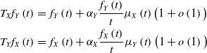 \begin{eqnarray*}T_{X}f_{Y}\left( t\right) &=&f_{Y}\left( t\right) +\alpha _{Y}\frac{f_{Y}\left( t\right) }{t}\mu _{X}\left( t\right) \big( 1+o\left( 1\right)\big) \\T_{Y}f_{X}\left( t\right) &=&f_{X}\left( t\right) +\alpha _{X}\frac{f_{X}\left( t\right) }{t}\mu _{Y}\left( t\right) \big( 1+o\left( 1\right)\big)\end{eqnarray*}
as $t\rightarrow \infty $
. In particular, if
$t\rightarrow \infty $
. In particular, if $\min\{\alpha _{X},\alpha _{Y}\}\gt2$
, as
$\min\{\alpha _{X},\alpha _{Y}\}\gt2$
, as $t\rightarrow \infty $
,
$t\rightarrow \infty $
,
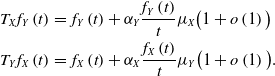 \begin{eqnarray*} T_{X}f_{Y}\left( t\right) &=&f_{Y}\left( t\right) +\alpha _{Y}\frac{ f_{Y}\left( t\right) }{t}\mu _{X}\big( 1+o\left( 1\right)\big) \\ T_{Y}f_{X}\left( t\right) &=&f_{X}\left( t\right) +\alpha _{X}\frac{ f_{X}\left( t\right) }{t}\mu _{Y} \big( 1+o\left( 1\right)\big) .\end{eqnarray*}
Proof. It is enough to establish the representation for $T_{Y}f_{X}$
. For
$T_{Y}f_{X}$
. For $\epsilon \gt0$
, as
$\epsilon \gt0$
, as $f_{X}$
is asymptotically smooth, there exists
$f_{X}$
is asymptotically smooth, there exists $\frac{1}{2}\gt\delta \gt0$
such that for all large t
$\frac{1}{2}\gt\delta \gt0$
such that for all large t
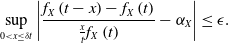 \begin{equation}\sup_{0 \lt x\leq \delta t}\left\vert \frac{f_{X}\left( t-x\right) -f_{X}\left(t\right) }{\frac{x}{t}f_{X}\left( t\right) }-\alpha _{X}\right\vert \leq\epsilon . \end{equation}
As in Barbe and Mc Cormick (Reference Barbe and McCormick2005), we write $T_{Y}f_{X}\left( t\right)-f_{X}\left( t\right) -\alpha _{X}\frac{f_{X}\left( t\right) }{t}\mu_{Y}\left( t\right) $
as a sum of four terms,
$T_{Y}f_{X}\left( t\right)-f_{X}\left( t\right) -\alpha _{X}\frac{f_{X}\left( t\right) }{t}\mu_{Y}\left( t\right) $
as a sum of four terms,
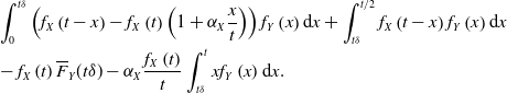 \begin{equation}\begin{aligned} &\int_{0}^{t \delta} \left(f_{X }\left( t-x\right) -f_{X}\left( t\right) \left(1+\alpha_X \frac{x}{t}\right)\right) f _{Y }\left(x\right) \mathrm{d} x +\int_{t \delta}^{t / 2} f_{X }\left( t-x\right) f_{Y }\left(x\right) \mathrm{d} x \\& -f_{X }\left( t\right)\overline{F}_{Y }(t \delta)- \alpha_X\frac{f_{X }\left( t\right)}{t} \int_{t \delta}^{t } x f_{Y}\left( x\right) \mathrm{d} x.\end{aligned}\end{equation}
Since $\frac{x}{t}f_{X}\left( t\right)$
is positive, we know from (B1) that for all
$\frac{x}{t}f_{X}\left( t\right)$
is positive, we know from (B1) that for all $0 \lt x\leq \delta t$
,
$0 \lt x\leq \delta t$
,
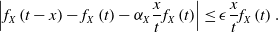 \begin{align*}\left\vert f_{X}\left( t-x\right) -f_{X}\left(t\right) -\alpha _{X}\frac{x}{t}f_{X}\left( t\right)\right\vert \leq\epsilon \frac{x}{t}f_{X}\left( t\right).\end{align*}
Therefore, the first term of (B2) is bounded by
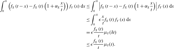 \begin{equation*} \begin{aligned}\int_{0}^{t \delta} \left(f_{X }\left( t-x\right) -f_{X }\left( t\right) \left(1+\alpha_X \frac{x}{t}\right)\right) f _{Y }\left( x\right) \mathrm{d} x &\leq \int_{0}^{t \delta} \left\vert f_{X }\left( t-x\right) -f_{X }\left( t\right) \left(1+\alpha_X \frac{x}{t}\right)\right\vert f _{Y }\left( x\right) \mathrm{d} x\\ &\leq \int_{0}^{t \delta} \epsilon \frac{x}{t}f_{X}\left( t\right) f _{Y }\left( x\right) \mathrm{d} x\\ &=\epsilon\frac{f_{X}\left( t\right)}{t} \mu_Y(\delta t)\\ &\leq \epsilon\frac{f_{X}\left( t\right)}{t} \mu_Y( t). \end{aligned}\end{equation*}
Let us consider $f^*_{X}\left( t\right) =\sup_{\frac{t}{2} \lt x \lt (1-\delta )t}f_{X}\left( x\right) $
. If
$f^*_{X}\left( t\right) =\sup_{\frac{t}{2} \lt x \lt (1-\delta )t}f_{X}\left( x\right) $
. If $t \delta\leq x\leq t / 2$
, then
$t \delta\leq x\leq t / 2$
, then $t/2\leq t-x\leq t (1-\delta)$
and
$t/2\leq t-x\leq t (1-\delta)$
and
 \begin{align*}\int_{t \delta}^{t / 2} f_{X }\left( t-x\right) f_{Y }\left(x\right) \mathrm{d} x\leq f^*_{X}\left( t\right)\int_{t \delta}^{t / 2} f_{Y }\left(x\right) \mathrm{d} x\leq f^*_{X}\left( t\right)\int_{t \delta}^{\infty} f_{Y }\left(x\right) \mathrm{d} x=\overline{F}_{Y}(\delta t) f^*_{X}\left( t\right).\end{align*}
Hence, (B2) can be bounded as follows:
 \begin{equation*} \begin{aligned} &T_{Y }f_{X }\left( t\right) -f_{X }\left( t\right) -\alpha_X \frac{f_{X }\left( t\right) }{t} \mu _{Y }\left( t\right)\\ &=\int_{0}^{t \delta} \left(f_{X }\left( t-x\right) -f_{X }\left( t\right) \left(1+\alpha_X \frac{x}{t}\right)\right) f _{Y }\left( x\right) \mathrm{d} x +\int_{t \delta}^{t / 2} f_{X }\left( t-x\right) f_{Y }\left( x\right) \mathrm{d} x \\ &\quad \quad -f_{X }\left( t\right)(\overline{F}_{Y }(t \delta))- \alpha_X \frac{f_{X }\left( t\right)}{t} \int_{t \delta}^{t } x f_{Y}\left( x\right) \mathrm{d} x\\ & \leq \frac{f_{X }\left( t\right)}{t}\mu_{Y }\left( t\right) \epsilon+\overline{F}_{Y}(\delta t)f^*_{X}\left( t\right)-f_{X }\left( t\right)\overline{F}_{Y }(t \delta)- \alpha_X \frac{f_{X }\left( t\right)}{t} \int_{t \delta}^{t } x f_{Y}\left( x\right) \mathrm{d} x \\ &= \alpha_X \frac{f_{X }\left( t\right)}{t} \left(\mu_{Y }\left( t\right) \frac{\epsilon}{\alpha_X}-\int_{t \delta}^{t } x f_{Y }\left( x\right) \mathrm{d} x\right)+\overline{F}_{Y }(\delta t)\left(f_{X }^*\left( t\right)-f_{X }\left( t\right)\right) \\ & = \alpha_X \frac{f_{X }\left( t\right)}{t} \mu_{Y }\left( t\right) \left( \frac{\epsilon}{\alpha_X}-\frac{1}{\mu_{Y }\left( t\right)}\int_{t \delta}^{t } x f_{Y }\left( x\right) \mathrm{d} x+\frac{\overline{F}_{Y }(\delta t)f_{X }^*\left( t\right) t}{\alpha_X f_{X }\left( t\right)\mu_{Y }\left( t\right)}-\frac{\overline{F}_{Y }(\delta t) t}{\alpha_X \mu_{Y }\left( t\right)}\right).\end{aligned}\end{equation*}
Therefore, the announced result follows if we can prove that
 \begin{equation}\frac{\epsilon }{\alpha _{X}}-\frac{1}{\mu _{Y}\left( t\right) }\int_{t\delta }^{t}xf_{Y}\left( x\right) \mathrm{d}x+\frac{\overline{F}_{Y}(\delta t)f^*_{X}\left( t\right) t}{\alpha _{X}f_{X}\left( t\right) \mu _{Y}\left(t\right) }-\frac{\overline{F}_{Y}(\delta t)t}{\alpha _{X}\mu _{Y}\left(t\right) }=o(1).\end{equation}
Since $f_X(\!\cdot\!)$
is regularly varying,
$f_X(\!\cdot\!)$
is regularly varying, $\overline{F}_{Y}(\delta t)$
is trivially
$\overline{F}_{Y}(\delta t)$
is trivially $O(\overline{F}_{Y}(t))$
. In addition, note that the convergence of slowly varying functions is uniform on compact sets (Bojanic and Seneta, Reference Bojanic and Seneta1971), that is, if L is a slowly varying function, then for every
$O(\overline{F}_{Y}(t))$
. In addition, note that the convergence of slowly varying functions is uniform on compact sets (Bojanic and Seneta, Reference Bojanic and Seneta1971), that is, if L is a slowly varying function, then for every $[a, b], 0 \lt a \lt b \lt \infty$
,
$[a, b], 0 \lt a \lt b \lt \infty$
, $\lim _{x \rightarrow+\infty} \sup _{a \leqslant \lambda \leqslant b}\left|\frac{L(\lambda x)}{L(x)}-1\right|=0$
. Since
$\lim _{x \rightarrow+\infty} \sup _{a \leqslant \lambda \leqslant b}\left|\frac{L(\lambda x)}{L(x)}-1\right|=0$
. Since $f_X(x)=x^{-\alpha_X}L_X(x)$
for a slowly varying function
$f_X(x)=x^{-\alpha_X}L_X(x)$
for a slowly varying function $L_X$
,
$L_X$
,
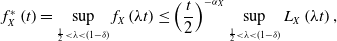 \begin{align*}f^*_{X}\left( t\right) =\sup_{\frac{1}{2} \lt \lambda \lt (1-\delta)}f_{X}\left( \lambda t\right)\leq \left(\frac{t}{2}\right)^{-\alpha_X}\sup_{\frac{1}{2}\lt\lambda\lt(1-\delta)}L_{X}\left( \lambda t\right),\end{align*}
and, therefore, $f^*_{X}\left( t\right)$
is
$f^*_{X}\left( t\right)$
is $O(f_{X}(t))$
. In consequence, (B3) holds if
$O(f_{X}(t))$
. In consequence, (B3) holds if
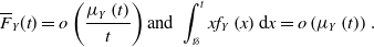 \begin{equation*}\overline{F}_{Y}(t)=o\left( \frac{\mu _{Y}\left( t\right) }{t}\right) \text{and }\int_{t\delta }^{t}x f_{Y}\left( x\right) \mathrm{d} x=o\left( \mu _{Y}\left(t\right) \right).\end{equation*}
Note that if $\mu_Y$
is finite (
$\mu_Y$
is finite ( $\alpha_Y\gt2$
), these assertions come as a direct consequence of Proposition 1.5.8 in Bingham et al. (Reference Bingham, Goldie and Teugels1987), which states that
$\alpha_Y\gt2$
), these assertions come as a direct consequence of Proposition 1.5.8 in Bingham et al. (Reference Bingham, Goldie and Teugels1987), which states that $\lim_{t\rightarrow\infty}\frac{t^2 f_Y(t)}{\mu_{Y}(t)}=-\alpha_Y+2$
, and the fact that
$\lim_{t\rightarrow\infty}\frac{t^2 f_Y(t)}{\mu_{Y}(t)}=-\alpha_Y+2$
, and the fact that $\bar{F}_Y(\!\cdot\!)$
is a regularly varying function with index
$\bar{F}_Y(\!\cdot\!)$
is a regularly varying function with index $\alpha_Y-1$
. Thus, we consider the case
$\alpha_Y-1$
. Thus, we consider the case $\alpha_Y=2$
. By Proposition 1.5.9.a in Bingham et al. (Reference Bingham, Goldie and Teugels1987),
$\alpha_Y=2$
. By Proposition 1.5.9.a in Bingham et al. (Reference Bingham, Goldie and Teugels1987), $\mu_Y(t)$
is slowly varying. Therefore,
$\mu_Y(t)$
is slowly varying. Therefore, $\int_{t\delta }^{t}xf_{Y}\left( x\right) \mathrm{d} x= \mu_Y(t) \left( 1-\frac{\mu_Y(\delta t)}{\mu_Y(t)}\right)=o(\mu_Y(t)).$
For
$\int_{t\delta }^{t}xf_{Y}\left( x\right) \mathrm{d} x= \mu_Y(t) \left( 1-\frac{\mu_Y(\delta t)}{\mu_Y(t)}\right)=o(\mu_Y(t)).$
For $\alpha_Y=2$
, Formula (1.5.8) in Bingham et al. (Reference Bingham, Goldie and Teugels1987) states that
$\alpha_Y=2$
, Formula (1.5.8) in Bingham et al. (Reference Bingham, Goldie and Teugels1987) states that $\frac{\mu_Y(t)}{t \bar{F}_Y(t)}\rightarrow\infty$
, and, hence
$\frac{\mu_Y(t)}{t \bar{F}_Y(t)}\rightarrow\infty$
, and, hence $\overline{F}_{Y}(t)=o\left( \frac{\mu _{Y}\left( t\right) }{t}\right)$
. The second assertion follows as
$\overline{F}_{Y}(t)=o\left( \frac{\mu _{Y}\left( t\right) }{t}\right)$
. The second assertion follows as $\min\{\alpha _{X},\alpha _{Y}\}\gt2$
implies that the random variables X and Y have finite first order moments.
$\min\{\alpha _{X},\alpha _{Y}\}\gt2$
implies that the random variables X and Y have finite first order moments.
C Proof of Corollary 5.3
Considering expression (5.1), we can obtain:
-
(1) If
$\alpha _{C_X}\gt\alpha _{C_Y}+2$
, then
$ f_{C_X}\left( s\right) =o(\frac{f_{C_Y}\left( s\right) }{s^2})$
. Hence, as
$s\rightarrow \infty $
,:
\begin{eqnarray*} m_{X}(s) &=&p_X \mu_{C_X}\frac{\frac{s f_{C_Y}\left( s\right) }{\mu_{C_Y}}\left( 1+\alpha _{C_Y}\frac{1}{s}(\frac{\sigma^2_{C_X}}{\mu_{C_X}}+\mu_{C_X})\left( 1+o\left( 1\right) \right) \right)+o(1)}{\frac{s f_{C_Y}\left( s\right)}{\mu_{C_Y}} \left( 1+\frac{p_X \mu_{C_X}}{s}\alpha _{C_Y}\left( 1+o\left( 1\right) \right) \right) +o(1)} \\ &=&p_X \mu_{C_X}\left( 1+ \frac{\alpha _{Y}\frac{1}{s}\frac{\sigma^2_{C_X}}{\mu_{C_X}}\left( 1+o\left( 1\right) \right) }{ 1+\frac{p_X \mu_{C_X}}{s}\alpha _{C_Y}\left( 1+o\left( 1\right) \right) }\right) \\ &=&p_X\mu _{C_X}\left( 1+\alpha _{C_Y}\frac{1}{s}\frac{\sigma^2_{C_X}}{\mu _{C_X}} \left( 1+o\left( 1\right) \right) \right) . \end{eqnarray*}
-
(2) If
$\alpha _{C_Y}+2\gt \alpha _{C_X}\gt\alpha _{C_Y}+1$
, then
$f_{C_X}\left( s\right) =o\left(\frac{f_{C_Y}\left( s\right)}{s}\right)$
and
$ f_{C_Y}\left( s\right) =o(s^2f_{C_X}\left( s\right) )$
. Hence, we can write:
\begin{eqnarray*} m_{X}(s) &=&\frac{\frac{f_{C_Y}\left( s\right) }{\mu_{C_Y}}\left( 1+\alpha _{C_Y}\frac{\mu_{\widetilde{C}_X}}{s}\left( 1+o\left( 1\right) \right) \right)+\frac{f_{C_X}\left( s\right)}{\mu_{C_X}} \left( \frac{s}{p_Y \mu_{C_Y}}+(\alpha _{C_X}-1)\left( 1+o\left( 1\right) \right) \right) }{\frac{f_{C_Y}\left( s\right)}{\mu_{C_Y}} \left( \frac{1}{p_X \mu_{C_X}}+\frac{\alpha _{C_Y}}{s}\left( 1+o\left( 1\right)\right)\right) +o\left(\frac{f_{C_Y}\left( s\right)}{s}\right)}\\ &=&p_X \mu_{C_X}\frac{\frac{f_{C_Y}\left( s\right) }{\mu_{C_Y}}\left( s+\alpha _{C_Y}\mu_{\widetilde{C}_X}\left( 1+o\left( 1\right) \right) \right)+s\frac{f_{C_X}\left( s\right)}{\mu_{C_X}} \left(\frac{s}{p_Y \mu_{C_Y}}+(\alpha _{C_X}-1)\left( 1+o\left( 1\right) \right) \right)}{\frac{f_{C_Y}\left( s\right)}{\mu_{C_Y}} \left( s+p_X \mu_{C_X}\alpha _{C_Y}\left( 1+o\left( 1\right)\right)\right)}\\ &=&p_X \mu_{C_X}\left(1+o(1)+\frac{s\frac{f_{C_X}\left( s\right)}{\mu_{C_X}} \left( \frac{s}{p_Y \mu_{C_Y}}+(\alpha _{C_X}-1)\left( 1+o\left( 1\right) \right) \right)}{\frac{f_{C_Y}\left( s\right)}{\mu_{C_Y}} \left( s+p_X \mu_{C_X}\alpha _{C_Y}\left( 1+o\left( 1\right)\right)\right)}\right)\\ &=&p_X \mu_{C_X}+s\frac{p_X}{p_Y}\frac{f_{C_X}\left( s\right)}{f_{C_Y}\left( s\right)} \left( 1+o\left( 1\right) \right). \end{eqnarray*}
-
(3-4) If
$\alpha _{C_Y}+1\gt\alpha _{C_X}\gt\alpha _{C_Y}$
, then, we can write: where
\begin{eqnarray*} m_{X}(s) &=&\frac{\frac{f_{C_Y}\left( s\right) }{\mu_{C_Y}}\left( 1+\alpha _{C_Y}\frac{\mu_{\widetilde{C}_X}}{s}\left( 1+o\left( 1\right) \right) \right)+\frac{f_{C_X}\left( s\right)}{\mu_{C_X}} \left( \frac{s}{p_Y \mu_{C_Y}}+(\alpha _{C_X}-1)\left( 1+o\left( 1\right) \right) \right) }{\frac{f_{C_Y}\left( s\right)}{\mu_{C_Y}} \left( \frac{1}{p_X \mu_{C_X}}+\frac{\alpha _{C_Y}}{s}\left( 1+o\left( 1\right)\right)\right) +\frac{f_{C_X}\left( s\right) }{\mu_{C_X}}\left(\frac{1}{p_Y \mu_{C_Y}}+\frac{\alpha _{C_X}}{s}\left( 1+o\left( 1\right) \right) \right)}\\ &=&s\;\frac{p_X }{p_Y }\;\frac{f_{C_X}(s) }{f_{C_Y}(s)}\frac{\frac{f_{C_Y}\left( s\right) }{f_{C_X}(s)\mu_{C_Y}} \frac{p_Y}{s}\left( 1+o\left( 1\right) \right) +\frac{1}{\mu_{C_X}} \left( \frac{1}{ \mu_{C_Y}}+\frac{p_Y(\alpha _{C_X}-1)}{s}\left( 1+o\left( 1\right) \right) \right) }{\frac{1}{\mu_{C_Y} \mu_{C_X}}+\frac{p_X\alpha _{C_Y}}{\mu_{C_Y}s}\left( 1+o\left( 1\right)\right) +\frac{f_{C_X}\left( s\right) }{f_{C_Y}\left( s\right)\mu_{C_X}}\left(\frac{p_X}{p_Y \mu_{C_Y}}+\frac{p_X\alpha _{C_X}}{s}\left( 1+o\left( 1\right) \right) \right)}\\ &=&s\;\frac{p_X }{p_Y }\;\frac{f_{C_X}(s) }{f_{C_Y}(s)}(1+r(s)). \notag\end{eqnarray*}
We can proceed analogously as in Proposition 4.7 and differ among the different frameworks. If
\begin{align*}r(s)=\frac{\frac{p_Y}{s}\frac{f_{C_Y}\left( s\right) }{f_{C_X}(s)\mu_{C_Y}} \left( 1+o\left( 1\right) \right)+\frac{1}{s}\left(\frac{p_Y(\alpha _{C_X}-1)}{\mu_{C_X}}-\frac{p_X \alpha_{C_Y}}{\mu_{C_Y}}\right)\left( 1+o\left( 1\right) \right)-\frac{p_X}{p_Y}\frac{f_{C_X}\left( s\right) }{f_{C_Y}\left( s\right)}\left(\frac{1}{ \mu_{C_Y}\mu_{C_X}}\left( 1+o\left( 1\right) \right) \right) }{ \frac{1}{ \mu_{C_Y}\mu_{C_X}}+\frac{p_X\alpha _{C_Y}}{s \mu_{C_Y}}\left( 1+o\left( 1\right)\right) +\frac{p_X}{p_Y}\frac{f_{C_X}\left( s\right) }{f_{C_Y}\left( s\right)}\left(\frac{1}{ \mu_{C_Y}\mu_{C_X}}+\frac{p_Y\alpha _{C_X}}{\mu_{C_X}s}\left( 1+o\left( 1\right) \right) \right)}.\end{align*}
$\alpha_{C_X}-\alpha_{C_Y}\gt \frac{1}{2}$
, then, the dominant term in the numerator is
$\frac{f_{C_Y}\left( s\right)}{s f_{C_X}\left( s\right)}$
and we can write
$r(s)=\frac{p_Y \mu_{C_X} f_{C_Y}\left( s\right)}{s f_{C_X}\left( s\right)}\left(1+o\left( 1\right) \right)$
. However, if
$\alpha_{C_X}-\alpha_{C_Y}\lt\frac{1}{2}$
, then the dominant term is
$\frac{f_{C_X}\left( s\right)}{f_{C_Y}\left( s\right)}$
and
$r(s)=-\frac{p_X}{p_Y}\frac{f_{C_X}\left( s\right)}{ f_{C_Y}\left( s\right)}\left(1+o\left( 1\right) \right)$
.
-
(5) If
$\alpha=\alpha _{C_Y}=\alpha _{C_X}$
and and
$f_{C_X}(s)=c f_{C_Y}(s)\left( 1+o\left( 1\right) \right)$
with
$c\gt0$
, then, we can write:
\begin{eqnarray*} m_{X}(s) &=&\frac{\frac{f_{C_Y}\left( s\right) }{\mu_{C_Y}}\left( 1+\alpha\frac{\mu_{\widetilde{C}_X}}{s}\left( 1+o\left( 1\right) \right) \right)+\frac{c f_{C_Y}(s)}{\mu_{C_X}} \left( \frac{s}{p_Y \mu_{C_Y}}+(\alpha-1) \right)\left( 1+o\left( 1\right) \right) }{\frac{f_{C_Y}\left( s\right)}{\mu_{C_Y}} \left( \frac{1}{p_X \mu_{C_X}}+\frac{\alpha}{s}\left( 1+o\left( 1\right)\right)\right) +\frac{c f_{C_Y}(s) }{\mu_{C_X}}\left(\frac{1}{p_Y \mu_{C_Y}}+\frac{\alpha}{s} \right)\left( 1+o\left( 1\right) \right)}\\ &=&s\;\frac{\frac{1 }{s \mu_{C_Y}}\left( 1+o\left( 1\right) \right) +\frac{c}{\mu_{C_X}} \left( \frac{1}{p_Y \mu_{C_Y}}+\frac{(\alpha-1)}{s} \right)\left( 1+o\left( 1\right) \right) }{\frac{1}{\mu_{C_Y}} \left( \frac{1}{p_X \mu_{C_X}}+\frac{\alpha}{s}\left( 1+o\left( 1\right)\right)\right) +\frac{c }{\mu_{C_X}}\left(\frac{1}{p_Y \mu_{C_Y}}+\frac{\alpha}{s} \right)\left( 1+o\left( 1\right) \right)}\\ &=& \frac{c}{\frac{p_Y}{p_X}+c}s\;\frac{\frac{\mu_{C_X}p_Y}{c\; s }\left( 1+o\left( 1\right) \right) + \left( 1+p_Y \mu_{C_Y}\frac{(\alpha-1)}{s} \right)\left( 1+o\left( 1\right) \right) }{ \left(1+\frac{\alpha}{s}\frac{p_Y \left(c\; \mu_{C_Y}+\mu_{C_X}\right)}{\frac{p_Y}{p_X}+c}\right)\left( 1+o\left( 1\right)\right) } \\ &=& \frac{c}{\frac{p_Y}{p_X}+c}s\left(1+\frac{1}{s}\frac{\frac{\mu_{C_X}p_Y}{c}\left( 1+o\left( 1\right) \right) + \left( p_Y \mu_{C_Y}(\alpha-1)\right)\left( 1+o\left( 1\right) \right)-\alpha\frac{p_Y \left(c\; \mu_{C_Y}+\mu_{C_X}\right)}{\frac{p_Y}{p_X}+c} }{ \left(1+\frac{\alpha}{s}\frac{p_Y \left(c\; \mu_{C_Y}+\mu_{C_X}\right)}{\frac{p_Y}{p_X}+c}\right)\left( 1+o\left( 1\right)\right) } \right) \\ &=& \frac{c}{\frac{p_Y}{p_X}+c}s\left(1+\frac{1}{s}\left(\frac{\mu_{C_X}p_Y}{c}-p_Y \mu_{C_Y}+\alpha\frac{p_Y}{\frac{p_Y}{p_X}+c} \left(\frac{p_Y}{p_X} \mu_{C_Y}-\mu_{C_X}\right) \right)\left( 1+o\left( 1\right)\right)\right) .\notag\end{eqnarray*}


D Extension to more than two terms in the sum
Until now, we have considered sums of two random variables X and Y. In applications to risk sharing, pools often comprise many participants so this section studies the non-decreasingness of conditional expectations given sums of n random variables. Precisely, let us consider n independent, nonnegative, and continuous random variables $X_1,X_2,\ldots,X_n$
with regularly varying densities. Let
$X_1,X_2,\ldots,X_n$
with regularly varying densities. Let $S_n=\sum_{i=1}^n X_i$
. Note that, under a risk-sharing pool considering the conditional mean risk rule, the contribution of the risk holder i,
$S_n=\sum_{i=1}^n X_i$
. Note that, under a risk-sharing pool considering the conditional mean risk rule, the contribution of the risk holder i, $m_i(s)=\mathrm{E}[X_i\mid S{_n}=s]$
, only depends on the pair
$m_i(s)=\mathrm{E}[X_i\mid S{_n}=s]$
, only depends on the pair $\left(X_i,S{_n}-X_i\right)$
. Since regularly varying densities are closed under convolutions,
$\left(X_i,S{_n}-X_i\right)$
. Since regularly varying densities are closed under convolutions, $S{_n}-X_i$
has a regularly varying density and, therefore, the results obtained in the bivariate framework can be extended to a higher dimensional setting. Formally, the following result states the closure under convolutions of random variables with regularly varying densities. Proceeding by induction, the result comes as a direct consequence of Theorem 2.1 in Bingham et al. (Reference Bingham, Goldie and Omey2006).
$S{_n}-X_i$
has a regularly varying density and, therefore, the results obtained in the bivariate framework can be extended to a higher dimensional setting. Formally, the following result states the closure under convolutions of random variables with regularly varying densities. Proceeding by induction, the result comes as a direct consequence of Theorem 2.1 in Bingham et al. (Reference Bingham, Goldie and Omey2006).
Corollary D.1. Let $f_{X_1},f_{X_2},\ldots,f_{X_n}$
be the probability density functions of
$f_{X_1},f_{X_2},\ldots,f_{X_n}$
be the probability density functions of $X_1,X_2,\ldots,X_n$
which are regularly varying with respective indices
$X_1,X_2,\ldots,X_n$
which are regularly varying with respective indices $\alpha_1,\alpha_2,\ldots, \alpha_n$
. If
$\alpha_1,\alpha_2,\ldots, \alpha_n$
. If $\alpha_j \lt \alpha_k,\text{ for} $
k j
$\alpha_j \lt \alpha_k,\text{ for} $
k j $ \text{, where }\alpha_j=\min\lbrace \alpha_1,\ldots, \alpha_n\rbrace$
, so that
$ \text{, where }\alpha_j=\min\lbrace \alpha_1,\ldots, \alpha_n\rbrace$
, so that $f_{X_k}(x)=\mathrm{o}(f_{X_j}(x))$
for
$f_{X_k}(x)=\mathrm{o}(f_{X_j}(x))$
for $k\neq j$
, then the convolution product
$k\neq j$
, then the convolution product $f_{X_1+X_2+\ldots+X_n}$
of
$f_{X_1+X_2+\ldots+X_n}$
of $f_{X_1},f_{X_2},\ldots,f_{X_n}$
satisfies
$f_{X_1},f_{X_2},\ldots,f_{X_n}$
satisfies
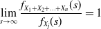 \begin{align*} \lim_{s\rightarrow \infty}\frac{f_{X_1+X_2+\ldots+X_n}(s)}{f_{X_j}(s)}=1 \end{align*}
and is a regularly varying density with index $\alpha_j$
.
$\alpha_j$
.
Let $S_n=\sum_{j=1}^{n} X_j$
be the total loss of the pool, where the subscript n emphasizes the number of economic agents forming the pool. The contribution paid ex post by participant i is
$S_n=\sum_{j=1}^{n} X_j$
be the total loss of the pool, where the subscript n emphasizes the number of economic agents forming the pool. The contribution paid ex post by participant i is $m_i(s)=\mathrm{E}[X_i\mid S_n=s]$
. We are now in a position to determine a sufficient condition for the existence of a sabotage opportunity.
$m_i(s)=\mathrm{E}[X_i\mid S_n=s]$
. We are now in a position to determine a sufficient condition for the existence of a sabotage opportunity.
Proposition D.2. Consider independent, nonnegative and continuous random variables $X_1, \ldots, X_n$
with regularly varying density functions
$X_1, \ldots, X_n$
with regularly varying density functions $f_{X_1},f_{X_2},\ldots,f_{X_n}$
having respective tail indices
$f_{X_1},f_{X_2},\ldots,f_{X_n}$
having respective tail indices $\alpha_1,\ldots, \alpha_n$
. Let us consider j(i) the index of the minimum tail index excluding
$\alpha_1,\ldots, \alpha_n$
. Let us consider j(i) the index of the minimum tail index excluding $\alpha_i$
. That is,
$\alpha_i$
. That is, $\alpha_{j(i)}\,:\!=\min\lbrace \alpha_1,\ldots \alpha_{i-1}, \alpha_{i+1}\ldots \alpha_n\rbrace$
and let us assume that
$\alpha_{j(i)}\,:\!=\min\lbrace \alpha_1,\ldots \alpha_{i-1}, \alpha_{i+1}\ldots \alpha_n\rbrace$
and let us assume that $\alpha_{j(i)}\lt\alpha_k$
for all
$\alpha_{j(i)}\lt\alpha_k$
for all $k\neq j(i)$
. If
$k\neq j(i)$
. If $\alpha_i \gt \alpha_{j(i)}+1$
then
$\alpha_i \gt \alpha_{j(i)}+1$
then
-
1.
$\lim_{s\rightarrow \infty}m_i(s)=\mathrm{E}[X_i]$
, -
2. there exists a nonempty interval in
$(0,\infty)$
where
$m_i(\!\cdot\!)$
is decreasing.


Proof. Using the representation of the conditional expectation given the sum in terms of size-biasing provided in Proposition 2.2 in Denuit (Reference Denuit2019), we can write
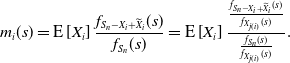 \begin{equation*} m_i(s) =\mathrm{E}\left[X_i\right] \frac{f_{S_n-X_i+\widetilde{X}_i}(s)}{f_{S_n}(s)}=\mathrm{E}\left[X_i\right] \frac{\frac{f_{S_n-X_i+\widetilde{X}_i}(s)}{f_{X_{j(i)}}(s)}}{\frac{f_{S_n}(s)}{f_{X_{j(i)}}(s)}}. \end{equation*}
Hence, by Corollary D.1,
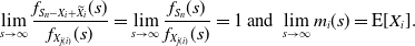 \begin{align*}\lim_{s\rightarrow \infty}\frac{f_{S_n-X_i+\widetilde{X}_i}(s)}{f_{X_{j(i)}}(s)}=\lim_{s\rightarrow \infty}\frac{f_{S_n}(s)}{f_{X_{j(i)}}(s)}=1\text{ and }\lim_{s\rightarrow \infty}m_i(s)=\mathrm{E}[X_i].\end{align*}
The latter assertion follows as in the proof of Proposition 3.3, taking into account that $m_{i}(0)=0$
,
$m_{i}(0)=0$
, $\lim_{s\rightarrow \infty }m_{i}(s)=\mathrm{E}\left[ X_i\right] $
and
$\lim_{s\rightarrow \infty }m_{i}(s)=\mathrm{E}\left[ X_i\right] $
and $\mathrm{E}[X_i]=\mathrm{E}[m_{i}(S_n)]$
. This ends the proof.
$\mathrm{E}[X_i]=\mathrm{E}[m_{i}(S_n)]$
. This ends the proof.
A direct consequence of this result is that once any two indices differ in more than one unit, there exists an index i such that $m_i(\!\cdot\!)$
decreases in an interval.
$m_i(\!\cdot\!)$
decreases in an interval.
Corollary D.3. Consider independent, nonnegative and continuous random variables $X_1, \ldots, X_n$
with regularly varying density functions having respective indices
$X_1, \ldots, X_n$
with regularly varying density functions having respective indices $\alpha_1,\ldots, \alpha_n$
. If there exists i and j(i) such that
$\alpha_1,\ldots, \alpha_n$
. If there exists i and j(i) such that $\alpha_{j(i)}=\min\lbrace \alpha_1,\ldots \alpha_{i-1}, \alpha_{i+1}\ldots \alpha_n\rbrace$
with
$\alpha_{j(i)}=\min\lbrace \alpha_1,\ldots \alpha_{i-1}, \alpha_{i+1}\ldots \alpha_n\rbrace$
with $\alpha_{j(i)}\lt\alpha_k$
for
$\alpha_{j(i)}\lt\alpha_k$
for $k\neq j(i)$
and
$k\neq j(i)$
and $\alpha_{j(i)}+1\lt\alpha_i$
, then there is an interval where
$\alpha_{j(i)}+1\lt\alpha_i$
, then there is an interval where $m_i(\!\cdot\!)$
is decreasing.
$m_i(\!\cdot\!)$
is decreasing.
Corollary D.3 indicates that in a pool where the risks $X_i$
have regularly varying densities, a necessary condition to avoid sabotage is to remove participants whose index differ by more than one unit from the others. The following example illustrates this situation.
$X_i$
have regularly varying densities, a necessary condition to avoid sabotage is to remove participants whose index differ by more than one unit from the others. The following example illustrates this situation.
Example D.4. Let us consider four independent random variables $X_i\sim P(I)(1, \alpha_i)$
(
$X_i\sim P(I)(1, \alpha_i)$
( $i=1,2,3,4$
) with
$i=1,2,3,4$
) with $\alpha_1=2.9$
,
$\alpha_1=2.9$
, $\alpha_2=1.6$
,
$\alpha_2=1.6$
, $\alpha_3=2.4$
,
$\alpha_3=2.4$
, $\alpha_4=2$
. Since
$\alpha_4=2$
. Since $\alpha_1\gt\alpha_2+1$
, we know from Proposition D.2 that there must be an interval where
$\alpha_1\gt\alpha_2+1$
, we know from Proposition D.2 that there must be an interval where $\mathrm{E}[X_1\mid S_4=s]$
decreases with s, which is indeed visible on Figure D1. Specifically, considering a pool with the four risks included, Figure D1 shows the contribution of each participant in terms of the total loss, where we can see that
$\mathrm{E}[X_1\mid S_4=s]$
decreases with s, which is indeed visible on Figure D1. Specifically, considering a pool with the four risks included, Figure D1 shows the contribution of each participant in terms of the total loss, where we can see that $\mathrm{E}[X_1\mid S_4=s]$
converges to
$\mathrm{E}[X_1\mid S_4=s]$
converges to $\mathrm{E}[X_1]$
and starts decreasing when
$\mathrm{E}[X_1]$
and starts decreasing when $S_4$
exceeds a threshold around 15. Therefore, the no-sabotage condition does not hold.
$S_4$
exceeds a threshold around 15. Therefore, the no-sabotage condition does not hold.
Functions $s\mapsto\mathrm{E}[X_i\mid S_4=s]$
for
$s\mapsto\mathrm{E}[X_i\mid S_4=s]$
for $i=1,2,3,4$
where
$i=1,2,3,4$
where $S_4=\sum_{i=1}^{4}X_i$
and
$S_4=\sum_{i=1}^{4}X_i$
and $X_i\sim P(I)(1, \alpha_i)$
with
$X_i\sim P(I)(1, \alpha_i)$
with $\alpha_1=2.9$
,
$\alpha_1=2.9$
, $\alpha_2=1.6$
,
$\alpha_2=1.6$
, $\alpha_3=2.4$
,
$\alpha_3=2.4$
, $\alpha_4=2$
.
$\alpha_4=2$
.

Removing either $X_1$
or
$X_1$
or $X_2$
from the pool so that no index differs by more than one unit from the others, there is no evidence of a sabotage scenario. The contributions in the new pools, without participant 1 or 2 appear in Figure D.4(a) and (b), and we can observe that, for these numerical examples, all contributions increase in the sum.
$X_2$
from the pool so that no index differs by more than one unit from the others, there is no evidence of a sabotage scenario. The contributions in the new pools, without participant 1 or 2 appear in Figure D.4(a) and (b), and we can observe that, for these numerical examples, all contributions increase in the sum.
Contributions considering $X_i\sim P(I)(1, \alpha_i)$
(
$X_i\sim P(I)(1, \alpha_i)$
( $i=1,2,3,4$
) with
$i=1,2,3,4$
) with $\alpha_1=2.9$
,
$\alpha_1=2.9$
, $\alpha_2=1.6$
,
$\alpha_2=1.6$
, $\alpha_3=2.4$
,
$\alpha_3=2.4$
, $\alpha_4=2$
where
$\alpha_4=2$
where $S_3=X_1+X_3+X_4$
and
$S_3=X_1+X_3+X_4$
and $S'_3=X_1+X_3+X_4$
.
$S'_3=X_1+X_3+X_4$
.
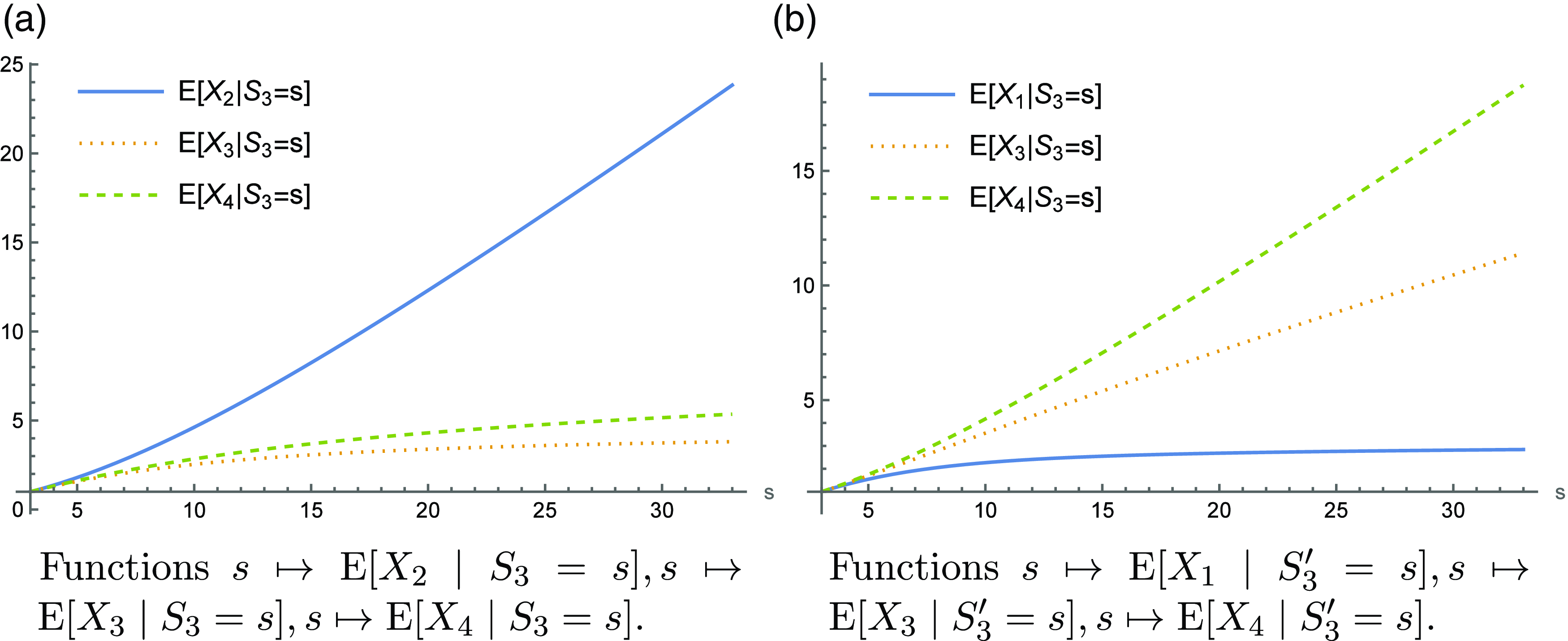
E Extension considering the Farlie–Gumbel–Morgenstern copula
The results obtained throughout the paper are based on the assumption that the random variables are independent. Consequently, their conclusions may not be directly applicable in scenarios where the random variables exhibit correlation. However, considering that the dependence structure between the variables follows a Farlie–Gumbel–Morgenstern (FGM) copula, it is still possible to study the asymptotic level of the conditional expectation. The FGM copula is a dependence structure that introduces only light dependence. However, it can serve to model both positive and negative dependence. Due to its simplicity and practical representations, the family of FGM copulas has been widely employed in risk management and in the actuarial literature (see, for instance, Bargès et al., Reference Bargès, Cossette, Loisel and Marceau2011 or Mao and Yang, Reference Mao and Yang2015). In particular, within a risk-sharing framework, in Blier-Wong et al. (Reference Blier-Wong, Cossette and Marceau2023), the expression of the contributions under the conditional mean risk-sharing rule is studied for vectors with mixed Erlang distributed marginals and the FGM copula. In addition, in Bargès et al. (Reference Bargès, Cossette and Marceau2009), TVaR-based insurance capital allocation is discussed for risks following exponential marginals and the FGM copula.
The FGM copula is defined as
 \begin{equation*}C(u,v)=uv\left[1+\lambda (1-v)(1-u)\right] \text{ for } u,v\in[0,1], \lambda\in[-1,1].\end{equation*}
The density is therefore given by
 \begin{equation*} c(u,v)=1+\lambda (1-2v)(1-2u) \text{ for } u,v\in[0,1], \lambda\in[-1,1].\end{equation*}
If X,Y have respective densities and survival functions given by $f_X,f_Y,\bar{F}_X,\bar{F}_Y$
and copula FGM with parameter
$f_X,f_Y,\bar{F}_X,\bar{F}_Y$
and copula FGM with parameter $ \lambda\in[-1,1]$
, then the joint density is given by
$ \lambda\in[-1,1]$
, then the joint density is given by
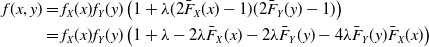 \begin{align} f(x,y)&=f_X(x)f_Y(y)\left(1+\lambda(2\bar{F}_X(x)-1)(2\bar{F}_Y(y)-1)\right)\nonumber\\ &=f_X(x)f_Y(y)\left(1+\lambda-2\lambda\bar{F}_X(x)-2\lambda\bar{F}_Y(y)-4\lambda\bar{F}_Y(y)\bar{F}_X(x)\right) \end{align}
For a random variable Z with regularly varying density, let us denote by $Z^{\ast}$
the random variable with density
$Z^{\ast}$
the random variable with density
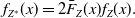 \begin{equation} f_{Z^{\ast}}(x)=2\bar{F}_Z(x)f_Z(x).\end{equation}
The density $f_{Z^{\ast}}(\!\cdot\!)$
is regularly varying with tail index
$f_{Z^{\ast}}(\!\cdot\!)$
is regularly varying with tail index $2\alpha-1$
. Considering
$2\alpha-1$
. Considering $X^{\ast}, Y^{\ast}$
the variables derived as described, the joint density of two variables X,Y with a FGM copula can be written as a linear combination of four joint densities of independent random variables,
$X^{\ast}, Y^{\ast}$
the variables derived as described, the joint density of two variables X,Y with a FGM copula can be written as a linear combination of four joint densities of independent random variables,
 \begin{equation}f(x,y)= (1+\lambda)f_X(x)f_Y(y)-\lambda f_{X^{\ast}}(x) f_Y(y) -\lambda f_{Y^{\ast}}(y) f_X(x)+\lambda f_{X^{\ast}}(x) f_{Y^{\ast}}(y).\end{equation}
Hence, we can extend some of the results derived under independence as follows.
Proposition E.1. Let (X,Y) be a random vector with an FGM copula with parameter $\lambda\in[\!-1,1]$
. Let X,Y posses regularly varying densities
$\lambda\in[\!-1,1]$
. Let X,Y posses regularly varying densities $f_X(\!\cdot\!)$
and
$f_X(\!\cdot\!)$
and $f_Y(\!\cdot\!)$
with respective indices
$f_Y(\!\cdot\!)$
with respective indices $\alpha _{X}$
and
$\alpha _{X}$
and $\alpha_Y$
verifying
$\alpha_Y$
verifying $\alpha_X\gt \alpha_Y$
and respective associated slowly varying functions
$\alpha_X\gt \alpha_Y$
and respective associated slowly varying functions $L_X(\!\cdot\!)$
and
$L_X(\!\cdot\!)$
and $L_Y(\!\cdot\!)$
. Let
$L_Y(\!\cdot\!)$
. Let $X^{\ast}$
be defined from X according to (E2).
$X^{\ast}$
be defined from X according to (E2).
-
(a) If
$\alpha_Y+1\gt\alpha_X\gt \alpha_Y$
, then
$m_{X}(s) \rightarrow\infty$
as s tends to infinity. -
(b) If
$\alpha_X\gt \alpha_Y+1$
then
$\lim_{s\rightarrow \infty }m_{X}(s)=(1+\lambda)\mathrm{E}[X]-\lambda \mathrm{E}[X^{\ast}]$
.


Proof. The conditional expectation is given by
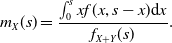 \begin{align*}m_X(s)=\frac{\int_{0}^{s}x f(x,s-x) \mathrm{d}x}{f_{X+Y}(s)}.\end{align*}
Let us denote by $X_I,Y_I$
two independent variables such that
$X_I,Y_I$
two independent variables such that $X_I\overset{\mathrm{d}}{=} X, Y_I\overset{\mathrm{d}}{=} Y$
. In a similar manner, we denote
$X_I\overset{\mathrm{d}}{=} X, Y_I\overset{\mathrm{d}}{=} Y$
. In a similar manner, we denote $X^{\ast}_I, Y^{\ast}_I$
the variables obtained as in (E2) to emphasize that they are independent. Then, using (E3), we have
$X^{\ast}_I, Y^{\ast}_I$
the variables obtained as in (E2) to emphasize that they are independent. Then, using (E3), we have
 \begin{equation}f_{X+Y}(s)= (1+\lambda)f_{X_I+Y_I}(s)-\lambda f_{X^{\ast}_I+Y_I}(s)-\lambda f_{Y^{\ast}_I+X_I}(s)+\lambda f_{X^{\ast}_I+Y^{\ast}_I}(s).\end{equation}
In a similar form
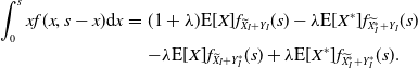 \begin{eqnarray}\int_{0}^{s}x f(x,s-x) \mathrm{d}x&=& (1+\lambda)\mathrm{E}[X] f_{\widetilde{X_I}+Y_I}(s)-\lambda \mathrm{E}[X^{\ast}]f_{\widetilde{X^{\ast}_I}+Y_I}(s) \nonumber\\& & -\lambda \mathrm{E}[X] f_{\widetilde{X_I}+Y^{\ast}_I}(s)+\lambda \mathrm{E}[X^{\ast}] f_{\widetilde{X^{\ast}_I}+Y^{\ast}_I}(s).\end{eqnarray}
Since the densities involved are regularly varying, taking (2.1) into account and since, for any random variable Z with regularly varying density, as s tends to infinity, $f_{Z^{\ast}}(s)=o(f_{Z}(s))$
, we can write
$f_{Z^{\ast}}(s)=o(f_{Z}(s))$
, we can write
 \begin{equation*} m_X(s)=\frac{\left((1+\lambda)\mathrm{E}[X]\left(f_{\widetilde{X_I}}(s)+f_{Y_I}(s)\right)-\lambda \mathrm{E}[X^{\ast}] f_{Y_I}(s)-\lambda \mathrm{E}[X] f_{\widetilde{X_I}}(s)\right)\left(1+o(1)\right)}{\left((1+\lambda)\left(f_{X_I}(s)+f_{Y_I}(s)\right)-\lambda f_{Y_I}(s)-\lambda f_{X_I}(s)\right)\left(1+o(1)\right)}.\end{equation*}
Similarly as in Proposition 3.7, we can conclude that, if $\alpha_Y+1\gt\alpha_X\gt \alpha_Y$
, then, as s tends to infinity,
$\alpha_Y+1\gt\alpha_X\gt \alpha_Y$
, then, as s tends to infinity, $f_{X_I}(s)=o(f_{Y_I}(s))$
and
$f_{X_I}(s)=o(f_{Y_I}(s))$
and $f_{Y_I}(s)=o(f_{\widetilde{X_I}}(s))$
and
$f_{Y_I}(s)=o(f_{\widetilde{X_I}}(s))$
and $m(s)\rightarrow \infty$
. Analogously as in Proposition 3.3, if
$m(s)\rightarrow \infty$
. Analogously as in Proposition 3.3, if $\alpha_X\gt \alpha_Y+1$
, then
$\alpha_X\gt \alpha_Y+1$
, then $f_{X_I}(s)=o(f_{Y_I}(s))$
and
$f_{X_I}(s)=o(f_{Y_I}(s))$
and $f_{\widetilde{X_I}}(s)=o(f_{Y_I}(s))$
and
$f_{\widetilde{X_I}}(s)=o(f_{Y_I}(s))$
and
 \begin{equation} \lim_{s\rightarrow \infty} m(s)= (1+\lambda)\mathrm{E}[X]-\lambda \mathrm{E}[X^{\ast}] .\end{equation}
Example E.2. Consider two random variables $X\sim P(I)(\theta_X, \alpha_X)$
and
$X\sim P(I)(\theta_X, \alpha_X)$
and $Y\sim P(I)(\theta_Y,\alpha_Y)$
with FGM copula with dependence parameter
$Y\sim P(I)(\theta_Y,\alpha_Y)$
with FGM copula with dependence parameter $\lambda\in[-1,1]$
and with
$\lambda\in[-1,1]$
and with $\alpha_X\gt\alpha_Y+1$
,
$\alpha_X\gt\alpha_Y+1$
, $\theta_X,\theta_Y\gt0$
. Then,
$\theta_X,\theta_Y\gt0$
. Then, $f_{X^{\ast}}(x)=\theta_X^{2\left(\alpha_X-1\right)}2\left(\alpha_X-1\right) x^{-2\alpha_X+1}$
,
$f_{X^{\ast}}(x)=\theta_X^{2\left(\alpha_X-1\right)}2\left(\alpha_X-1\right) x^{-2\alpha_X+1}$
, $X^{\ast} \sim P(I)(\theta_X, 2\alpha_X-1),$
and by (E6):
$X^{\ast} \sim P(I)(\theta_X, 2\alpha_X-1),$
and by (E6):
 \begin{align*}\lim_{s\rightarrow \infty}m_X(s)= (1+\lambda)\mathrm{E}[X]-\lambda \mathrm{E}[X^{\ast}].\end{align*}
Figure E1 shows the asymptotic level of $m_X(\!\cdot\!)$
considering
$m_X(\!\cdot\!)$
considering $\theta_X=\theta_Y=1$
,
$\theta_X=\theta_Y=1$
, $\lambda=-0.5$
,
$\lambda=-0.5$
, $\alpha_X=7 $
and
$\alpha_X=7 $
and $\alpha_Y=3 $
. E
$\alpha_Y=3 $
. E
Conditional expectation $m_X(\!\cdot\!)$
when
$m_X(\!\cdot\!)$
when $X\sim P(I)(\theta_X, \alpha_X)$
and
$X\sim P(I)(\theta_X, \alpha_X)$
and $Y\sim P(I)(\theta_Y,\alpha_Y)$
with FGM copula with dependence parameter
$Y\sim P(I)(\theta_Y,\alpha_Y)$
with FGM copula with dependence parameter $\lambda$
with
$\lambda$
with $\theta_X=\theta_Y=1$
,
$\theta_X=\theta_Y=1$
, $\lambda=-0.5$
,
$\lambda=-0.5$
, $\alpha_X=7 $
and
$\alpha_X=7 $
and $\alpha_Y=3 $
.
$\alpha_Y=3 $
.
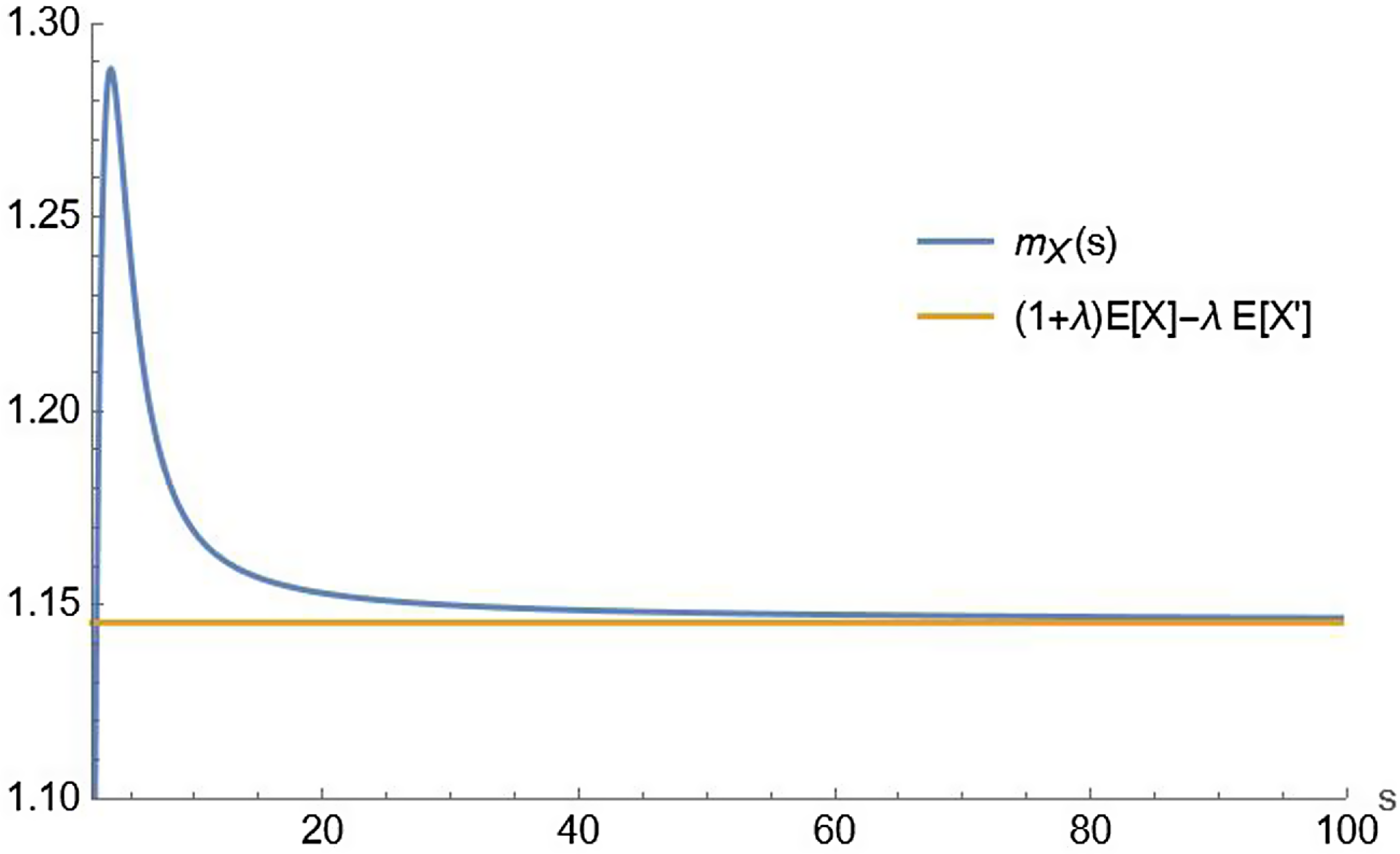
Let us remark that
 \begin{align*}\mathrm{E}[X^{\ast}]=2 \mathrm{E}[X] \int_{0}^{\infty}P[X\gt x]\frac{x}{\mathrm{E}[X]} f(x) \mathrm{d}x= 2 \mathrm{E}[X] P[X\gt\widetilde{X}].\end{align*}
Therefore, the limit in Proposition E.1(b) can also be written as
 \begin{equation}(1+\lambda)\mathrm{E}[X]-\lambda \mathrm{E}[X^{\ast}]=\mathrm{E}[X]\left(1+\lambda\left(1-2P[X\gt\widetilde{X}]\right)\right).\end{equation}
It is direct to see, as $X \preceq_{\mathrm{LR}} \widetilde{X}$
, where
$X \preceq_{\mathrm{LR}} \widetilde{X}$
, where $\preceq_{\mathrm{LR}}$
stands for the likelihood ratio order (see Shaked and Shanthikumar, Reference Shaked and Shanthikumar2007), that
$\preceq_{\mathrm{LR}}$
stands for the likelihood ratio order (see Shaked and Shanthikumar, Reference Shaked and Shanthikumar2007), that $\mathrm{P}[X\gt\widetilde{X}]\leq \frac{1}{2}$
and, therefore,
$\mathrm{P}[X\gt\widetilde{X}]\leq \frac{1}{2}$
and, therefore, $\left(1-2\mathrm{P}[X\gt\widetilde{X}]\right) \geq 0$
. Intuitively, if X is a random variable with regularly varying density and tail index
$\left(1-2\mathrm{P}[X\gt\widetilde{X}]\right) \geq 0$
. Intuitively, if X is a random variable with regularly varying density and tail index $\alpha_X$
, considering a greater
$\alpha_X$
, considering a greater $\alpha_X$
would imply that
$\alpha_X$
would imply that $\widetilde{X}$
is more similar to X and, therefore,
$\widetilde{X}$
is more similar to X and, therefore, $\mathrm{P}[X\gt\widetilde{X}]$
approaches
$\mathrm{P}[X\gt\widetilde{X}]$
approaches $\frac{1}{2}$
. For instance, if
$\frac{1}{2}$
. For instance, if $X\sim P(I)(\theta, \alpha_X)$
, then
$X\sim P(I)(\theta, \alpha_X)$
, then $\mathrm{P}[X\gt\widetilde{X}]=\frac{\alpha_X-1}{2 \alpha{_X}-1}$
, which converges to
$\mathrm{P}[X\gt\widetilde{X}]=\frac{\alpha_X-1}{2 \alpha{_X}-1}$
, which converges to $\frac{1}{2}$
as
$\frac{1}{2}$
as $\alpha_X$
tends to infinity. Therefore, we can intuitively expect that for variables with heavier tails, the dependence parameter has less influence on the limit in Proposition E.1(b) because the term
$\alpha_X$
tends to infinity. Therefore, we can intuitively expect that for variables with heavier tails, the dependence parameter has less influence on the limit in Proposition E.1(b) because the term $\left(1-2P[X\gt\widetilde{X}]\right)$
is smaller.
$\left(1-2P[X\gt\widetilde{X}]\right)$
is smaller.
Since $\left(1-2P[X\gt\widetilde{X}]\right)\geq 0$
, if
$\left(1-2P[X\gt\widetilde{X}]\right)\geq 0$
, if $\lambda\leq 0$
, then
$\lambda\leq 0$
, then $\mathrm{E}[X]\left(1+\lambda\left(1-2\mathrm{P}[X\gt\widetilde{X}]\right)\right)\leq \mathrm{E}[X]$
and proceeding as in Proposition 3.3, if
$\mathrm{E}[X]\left(1+\lambda\left(1-2\mathrm{P}[X\gt\widetilde{X}]\right)\right)\leq \mathrm{E}[X]$
and proceeding as in Proposition 3.3, if $\alpha_X\gt \alpha_Y+1$
, there exists a nonempty interval in
$\alpha_X\gt \alpha_Y+1$
, there exists a nonempty interval in $\left(0,\infty\right)$
where
$\left(0,\infty\right)$
where $m_X(\!\cdot\!)$
is decreasing. On the other hand, if
$m_X(\!\cdot\!)$
is decreasing. On the other hand, if $\lambda\gt0$
, we cannot ensure the existence of a non-empty interval but, since the limit is finite,
$\lambda\gt0$
, we cannot ensure the existence of a non-empty interval but, since the limit is finite, $m_X(\!\cdot\!)$
is necessarily bounded. Under the framework of a risk-sharing pool, this means that, even if we cannot guarantee the existence of a sabotage scenario, the risk holder of X may exaggerate the loss up to infinity with no great consequence (as their contribution is bounded). Similarly to the sabotage framework, this would neither be a desirable characteristic of a risk-sharing scheme. Therefore, if the dependence among risks follows an FGM copula, we can obtain similar conclusions as in the independence framework. Under this dependence structure, it is neither advisable to form risk-sharing pools when the tail indexes of the densities involved differ in more than one unit.
$m_X(\!\cdot\!)$
is necessarily bounded. Under the framework of a risk-sharing pool, this means that, even if we cannot guarantee the existence of a sabotage scenario, the risk holder of X may exaggerate the loss up to infinity with no great consequence (as their contribution is bounded). Similarly to the sabotage framework, this would neither be a desirable characteristic of a risk-sharing scheme. Therefore, if the dependence among risks follows an FGM copula, we can obtain similar conclusions as in the independence framework. Under this dependence structure, it is neither advisable to form risk-sharing pools when the tail indexes of the densities involved differ in more than one unit.


 Open access