





1. Introduction
The importance of ventilation in reducing the indoor transmission of infectious diseases was first highlighted by Nightingale [Reference Nightingale31]. When an infectious person breathes, talks, coughs or sneezes, disease-carrying particles are emitted. In poorly ventilated spaces, small particles known as aerosols can remain airborne for several hours, transmitting the disease to susceptible people when inhaled. During the COVID-19 pandemic, a key shift in understanding and mitigating transmission of the SARS-CoV-2 virus was the recognition of airborne transmission [Reference Morawska and Milton29], most likely responsible for superspreader outbreaks in a restaurant [Reference Ho19, Reference Lu26], courtroom [Reference Vernez, Schwarz, Sauvain, Petignat and Suarez35], choir practice [Reference Miller28] and meat processing plant [Reference Günther16].
There are two main approaches to modelling airborne transmission: Wells–Riley models and computational fluid dynamics (CFD). Wells–Riley models [Reference Riley, Murphy and Riley32] assume a well-mixed room, meaning aerosols are instantaneously transported throughout the room. Due to its high computational speed, this approach can be readily applied throughout an epidemic; this was the case for COVID-19 [Reference Buonanno, Stabile and Morawska6, Reference Dai and Zhao9, Reference Lelieveld24]. However, the well-mixed-room assumption is not always appropriate and neglects the spatial variation of the concentration around the room. One benefit of this approach is its broad applicability – results do not depend on the specific configuration of people, furniture and ventilation.
CFD models, on the other hand, simulate the detailed airflow in a room with a specific layout. The computational demand is high, so many CFD studies at the start of the COVID-19 pandemic focused on relatively short time frames (less than 5 minutes) [Reference Shafaghi, Rokhsar, Koşar and Ghorbani33, Reference Vuorinen36]. This simulation time is appropriate for heavier virus-laden droplets that quickly fall to the ground, but untenable for airborne transmission, which typically occurs over hours. Some CFD models have simulated aerosol evolution for up to an hour [Reference Shao, Zhou and He34], but the high computational times mean that CFD has a limited role in informing up-to-date decisions in a quickly developing epidemic. One key advantage of CFD models is in exploring a transmission event after-the-fact [Reference Ho19] to better understand the mechanisms influencing transmission.
Lau et al. [Reference Lau, Griffiths, English and Kaouri23] model the spatiotemporal evolution of aerosols in a room using an advection–diffusion–reaction (ADR) equation under the assumption of a recirculating airflow generated by an air-conditioning (AC) vent. Extending the Wells–Riley model, the Lau et al. [Reference Lau, Griffiths, English and Kaouri23] model accounts for the spatial variation of concentration and infection risk. Moreover, the airflow can be reduced to a 2D flow, which allows fast simulations, so the model can be quickly deployed in a fast-changing epidemic. Aerosol removal by ventilation is modelled as a global sink, as in the Wells–Riley type models. Under this assumption, good agreement with real-life scenarios ventilated by inbuilt AC units was obtained [Reference Lau, Griffiths, English and Kaouri23].
For rooms with poor or non-existent ventilation, air purifiers can increase overall aerosol removal. The effectiveness of air purifiers depends strongly on their location [Reference Burgmann and Janoske7, Reference Narayanan and Yang30], an effect that cannot be captured by the Wells–Riley model or the model of Lau et al. [Reference Lau, Griffiths, English and Kaouri23]. Moreover, many CFD studies of air purifiers report prohibitively long computational times; for example, Dbouk et al. [Reference Dbouk, Roger and Drikakis11] report 7 days to simulate a 2.5-minute event in a domestic setting. While air purifiers are not technically classified as ventilation, since they do not provide fresh air from outdoors, the American Society of Heating, Refrigeration and Air-Conditioning (ASHRAE) incorporates air cleaning devices in their measure of equivalent clean airflow when risk of disease transmission is high (e.g. during an epidemic) [4]. In the present study, following ASHRAE, we conflate air purifiers with ventilation since we are solely interested in aerosol removal. However, we note that relying only on air purifiers with no outdoor air exchange can result in a buildup of carbon dioxide, degrading the indoor air quality. The efficacy of an air purifier is described by the clean air delivery rate (CADR), which is a combination of the filter efficacy and the volumetric flow rate through the device.
In this paper, we introduce spatially localised ventilation to the modelling framework of Lau et al. [Reference Lau, Griffiths, English and Kaouri23]. While all ventilation systems (including doors, windows and AC units) have local effects, we are motivated by air purifiers; we introduce a cylindrical device that draws air in through the top and expels clean air from the bottom. This device is placed in addition to an inbuilt, poorly performing AC unit.
The model allows quick investigation of transmission events over long periods of time. Lectures, meetings, school lessons and certain time-limited social events (e.g. escape rooms) usually last for about an hour. Significantly more time is spent in restaurants, art galleries, networking events (e.g. conferences and workshops) and other social settings (e.g. pub quizzes). These scenarios are common transmission events for airborne diseases. We consider 1- and 4-hour events to explore the effectiveness of air purifiers in such settings.
The paper is organised as follows. The modelling framework, incorporating a local ventilation system, is presented in Section 2. In Section 3, we compare the average aerosol concentration in the room predicted by the local and global ventilation models. The spatial distribution of aerosols is then compared in Section 4. In Section 5, we compare the infection risk at specific locations arising from the two ventilation models. Conclusions and suggestions for future work are provided in Section 6.
2. Modelling framework
2.1. Global ventilation models
Prior to detailing the modelling framework of the present study, a brief overview of two pertinent models is provided. First, we describe the Wells–Riley model. The spatiotemporal generalisation of this model implemented by Lau et al. [Reference Lau, Griffiths, English and Kaouri23] is then described.
The Wells–Riley model and its variants [Reference Gammaitoni and Nucci15, Reference Miller28] assume a well-mixed room, meaning the aerosol concentration is spatially uniform and depends only on time, $t$
. The aerosol concentration in the room,
$t$
. The aerosol concentration in the room, $\mathcal{C}(t)$
, is thus governed by the ODE
$\mathcal{C}(t)$
, is thus governed by the ODE
 \begin{equation} \frac {\mathrm{d} \mathcal{C}}{\mathrm{d} t} = \frac {R}{V} - (\lambda + \beta + \sigma ) \mathcal{C}. \end{equation}
This closely matches the formulation used by Miller [Reference Miller28]. The first term on the right-hand side describes aerosol production as a global source, with $R$
denoting the rate at which aerosols are produced and
$R$
denoting the rate at which aerosols are produced and $V$
being the room volume. The second term on the right-hand side describes first-order removal of aerosols through a global sink, where each coefficient is the rate at which aerosols are removed by ventilation (
$V$
being the room volume. The second term on the right-hand side describes first-order removal of aerosols through a global sink, where each coefficient is the rate at which aerosols are removed by ventilation ( $\lambda$
), biological deactivation (
$\lambda$
), biological deactivation ( $\beta$
) and gravitational settling (
$\beta$
) and gravitational settling ( $\sigma$
).
$\sigma$
).
Parameters and their values
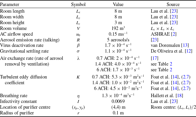
Table 1. Long description
A table with 12 rows and 4 columns. The columns are labeled Parameter, Symbol, Value, and Source. The table lists various parameters related to a room and airflow study, including room dimensions, airflow speed, aerosol emission rate, virus deactivation rate, gravitational settling rate, air exchange rate, turbulent eddy diffusion coefficient, breathing rate, infectivity constant, location of purifier center, and radius of purifier. Each row provides the symbol, value, and source for each parameter. For example, Room length is listed with a value of 8 meters from Lau et al. [23], Room width is also 8 meters from the same source, and Room height is 3 meters. The table includes specific values for rates and coefficients, such as the aerosol emission rate of 5 aerosols per second and the virus deactivation rate of 1.7 times 10 to the power of -4 per second.
In addition to (2.1), Wells–Riley models relate the aerosol concentration to the probability that a susceptible person becomes infected. Following Riley et al. [Reference Riley, Murphy and Riley32], the infection risk can be related to the concentration according to
 \begin{equation} P(t) = 1 - \exp \left [ - I \int _0^t \eta \mathcal{C}(\tau ) \, \mathrm{d} \tau \right ], \end{equation}
where $I$
describes the infectivity of the disease and
$I$
describes the infectivity of the disease and $\eta$
is a breathing rate (see Table 1 for units and values).
$\eta$
is a breathing rate (see Table 1 for units and values).
In order to capture the spatiotemporal evolution of aerosol concentration and infection risk, Lau et al. [Reference Lau, Griffiths, English and Kaouri23] generalised (2.1) to account for spatial effects: advection of aerosols around a recirculating AC flow and diffusion due to turbulent eddies. This results in an ADR equation governing the 2D concentration around the recirculating loop, $\mathscr{C}$
. This is an areal concentration (in aerosols/m
$\mathscr{C}$
. This is an areal concentration (in aerosols/m $^2$
), with different units to the volumetric concentration
$^2$
), with different units to the volumetric concentration $\mathcal{C}$
(in aerosols/m
$\mathcal{C}$
(in aerosols/m $^3$
) introduced above. The production term is modified so that an infected person is modelled as a point source at location
$^3$
) introduced above. The production term is modified so that an infected person is modelled as a point source at location $(x_0,y_0)$
, i.e.
$(x_0,y_0)$
, i.e. $R/V \rightarrow R \delta (x-x_0) \delta (y-y_0)$
. As in (2.1), the removal terms are treated as global sinks.
$R/V \rightarrow R \delta (x-x_0) \delta (y-y_0)$
. As in (2.1), the removal terms are treated as global sinks.
The Lau et al. [Reference Lau, Griffiths, English and Kaouri23] model was validated against two superspreader outbreaks: one in a courtroom in Switzerland [Reference Vernez, Schwarz, Sauvain, Petignat and Suarez35] and one in a restaurant in Guangzhou, China [Reference Li25, Reference Lu26]. In both cases, the results agreed well with real-world observations. For both scenarios, the transport of aerosols was dominated by a recirculating airflow generated by AC units that were ineffective at removing aerosols.
In this paper, we introduce a local treatment of ventilation in addition to the global sink used in both Wells–Riley models (2.1) and Lau et al. [Reference Lau, Griffiths, English and Kaouri23]. The modelling framework detailed below is a generalisation of the Lau et al. [Reference Lau, Griffiths, English and Kaouri23] framework. The assumptions that recover the Lau et al. [Reference Lau, Griffiths, English and Kaouri23] model are highlighted after the current model is described.
2.2. Spatiotemporal model with local ventilation
Consider a three-dimensional (3D) room of volume $V$
, with dimensions
$V$
, with dimensions $L_x$
,
$L_x$
, $L_y$
,
$L_y$
, $L_z$
, as depicted in Figure 1(a) (values given in Table 1). Following Lau et al. [Reference Lau, Griffiths, English and Kaouri23], we assume a recirculating flow produced by a single AC vent along the top corner and introduce the arclength coordinate
$L_z$
, as depicted in Figure 1(a) (values given in Table 1). Following Lau et al. [Reference Lau, Griffiths, English and Kaouri23], we assume a recirculating flow produced by a single AC vent along the top corner and introduce the arclength coordinate $\xi$
, which follows the recirculating loop. This assumption is consistent with the real-life case studies [Reference Li25, Reference Vernez, Schwarz, Sauvain, Petignat and Suarez35] with which Lau et al. [Reference Lau, Griffiths, English and Kaouri23] validated their model. Moreover, van Hooff et al. [Reference van Hooff, Blocken, Defraeye, Carmeliet and Van Heijst20] measure the flow generated by a similar AC configuration and observe a recirculating flow throughout the majority of the room. Additional flow features are also reported by van Hooff et al. [Reference van Hooff, Blocken, Defraeye, Carmeliet and Van Heijst20], such as a fast-moving jet near the ceiling and a counter-rotating loop near the top corner opposite the AC unit, both of which are confined to the top 15% of the room (
$\xi$
, which follows the recirculating loop. This assumption is consistent with the real-life case studies [Reference Li25, Reference Vernez, Schwarz, Sauvain, Petignat and Suarez35] with which Lau et al. [Reference Lau, Griffiths, English and Kaouri23] validated their model. Moreover, van Hooff et al. [Reference van Hooff, Blocken, Defraeye, Carmeliet and Van Heijst20] measure the flow generated by a similar AC configuration and observe a recirculating flow throughout the majority of the room. Additional flow features are also reported by van Hooff et al. [Reference van Hooff, Blocken, Defraeye, Carmeliet and Van Heijst20], such as a fast-moving jet near the ceiling and a counter-rotating loop near the top corner opposite the AC unit, both of which are confined to the top 15% of the room ( $z \gt 2.55$
m here). These flow features are neglected from the current modelling framework since we assume that aerosols are produced at head height (
$z \gt 2.55$
m here). These flow features are neglected from the current modelling framework since we assume that aerosols are produced at head height ( $\approx 1.5$
m, half the height of the room), so these near-ceiling structures are assumed to have a negligible effect on aerosol transport.
$\approx 1.5$
m, half the height of the room), so these near-ceiling structures are assumed to have a negligible effect on aerosol transport.
Parameters for two purifiers, with $\lambda = 2\times 10^{-4}$
s
$\lambda = 2\times 10^{-4}$
s $^{-1}$
(0.7 ACH)
$^{-1}$
(0.7 ACH)
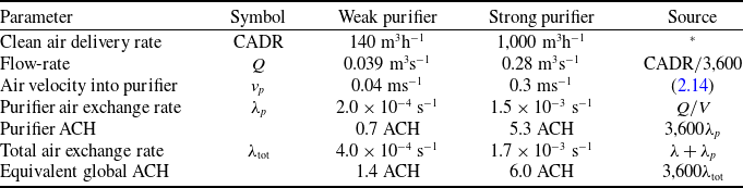
Table 2. Long description
A table comparing parameters for two purifiers. The table has 11 rows and 5 columns. The columns are labeled Parameter, Symbol, Weak purifier, Strong purifier, and Source. The rows list various parameters such as Clean air delivery rate, Flow-rate, Air velocity into purifier, Purifier air exchange rate, Purifier ACH, Total air exchange rate, and Equivalent global ACH. Each row provides specific values for the weak and strong purifiers, along with the source of the data. For example, the Clean air delivery rate (CADR) is 140 cubic meters per hour for the weak purifier and 1000 cubic meters per hour for the strong purifier. The Flow-rate (Q) is 0.039 cubic meters per second for the weak purifier and 0.28 cubic meters per second for the strong purifier. The Air velocity into purifier (vp) is 0.04 meters per second for the weak purifier and 0.3 meters per second for the strong purifier. The Purifier air exchange rate (λp) is 2.0 times 10 to the power of negative 4 per second for the weak purifier and 1.5 times 10 to the power of negative 3 per second for the strong purifier. The Purifier ACH is 0.7 ACH for the weak purifier and 5.3 ACH for the strong purifier. The Total air exchange rate (λtot) is 4.0 times 10 to the power of negative 4 per second for the weak purifier and 1.7 times 10 to the power of negative 3 per second for the strong purifier. The Equivalent global ACH is 1.4 ACH for the weak purifier and 6.0 ACH for the strong purifier.
* Weak purifier: Dbouk et al. [Reference Dbouk, Roger and Drikakis11], Strong purifier: Kähler et al. [Reference Kähler, Fuchs and Hain21].
A 3D room with dimensions $L_x$
,
$L_x$
, $L_y$
,
$L_y$
, $L_z$
is shown in (a). A cylindrical local ventilation system crosses the two recirculating layers and the arclength coordinate
$L_z$
is shown in (a). A cylindrical local ventilation system crosses the two recirculating layers and the arclength coordinate $\xi$
follows the recirculating loop. The computational domain
$\xi$
follows the recirculating loop. The computational domain $(\xi ,y)$
is shown in (b).
$(\xi ,y)$
is shown in (b).

The distance between the recirculation layers is taken to be $L_z/2$
, and the total arclength is assumed to be
$L_z/2$
, and the total arclength is assumed to be $2L_x$
(as in Lau et al. [Reference Lau, Griffiths, English and Kaouri23]). The height and arclength of the recirculating loop were determined by inspection of the recirculating flow reported by van Hooff et al. [Reference van Hooff, Blocken, Defraeye, Carmeliet and Van Heijst20].
$2L_x$
(as in Lau et al. [Reference Lau, Griffiths, English and Kaouri23]). The height and arclength of the recirculating loop were determined by inspection of the recirculating flow reported by van Hooff et al. [Reference van Hooff, Blocken, Defraeye, Carmeliet and Van Heijst20].
The local ventilation system employed here is inspired by a common purifier design – a cylindrical device that draws air in through the top and expels air radially outwards near the bottom [Reference Dbouk, Roger and Drikakis11]. Inside the device, air passes through a filter which traps entrained particles. The filter efficacy $\zeta$
is the proportion of particles that are trapped by the filter, and hence removed from the room. We will assume that no aerosols that pass through the purifier re-enter the room, so
$\zeta$
is the proportion of particles that are trapped by the filter, and hence removed from the room. We will assume that no aerosols that pass through the purifier re-enter the room, so $\zeta = 1$
. This assumption is common in purifier modelling [Reference Burgmann and Janoske7, Reference Dbouk, Roger and Drikakis11].
$\zeta = 1$
. This assumption is common in purifier modelling [Reference Burgmann and Janoske7, Reference Dbouk, Roger and Drikakis11].
We will denote the radius of this device by $r$
and assume that it extends over both recirculating layers: air is drawn into an inlet in the upper layer and expelled from an outlet in the lower layer.
$r$
and assume that it extends over both recirculating layers: air is drawn into an inlet in the upper layer and expelled from an outlet in the lower layer.
Figure 1(b) shows the computational domain $(\xi ,y)$
. The left/right halves correspond to the upper/lower layers and the purifier inlet and outlet appear as circles removed from the domain, with boundaries
$(\xi ,y)$
. The left/right halves correspond to the upper/lower layers and the purifier inlet and outlet appear as circles removed from the domain, with boundaries
 \begin{equation} \partial _{\mathrm{in}} = \{(\xi ,y) \,:\, |(\xi ,y) - (x_p,y_p)| = r\}, \end{equation}
 \begin{equation} \partial _{\mathrm{out}} = \{ (\xi ,y) \,:\, |(\xi ,y) - (2L_x-x_p,y_p)| = r\}, \end{equation}
where $(x_p,y_p)$
denotes the location of the centre of the purifier in the
$(x_p,y_p)$
denotes the location of the centre of the purifier in the $(x,y)$
-plane, and we will assume throughout this work that the purifier is in the centre of the room.
$(x,y)$
-plane, and we will assume throughout this work that the purifier is in the centre of the room.
In this quasi-3D model, the device extends the entire height of the room, which is significantly taller than real-life purifiers. This simplification allows for a comparison with the model of Lau et al. [Reference Lau, Griffiths, English and Kaouri23] while still offering useful and practical insights into the local effects of air purifiers.
Consider a single infectious individual at $\boldsymbol{x}_0 = (x_0,y_0)$
and talking continuously. Talking produces around 10 times as many aerosols as breathing [Reference Asadi, Wexler, Cappa, Barreda, Bouvier and Ristenpart1]: a reasonable worst-case scenario for an asymptomatic person. The infectious source will be placed in the top recirculating loop (
$\boldsymbol{x}_0 = (x_0,y_0)$
and talking continuously. Talking produces around 10 times as many aerosols as breathing [Reference Asadi, Wexler, Cappa, Barreda, Bouvier and Ristenpart1]: a reasonable worst-case scenario for an asymptomatic person. The infectious source will be placed in the top recirculating loop ( $\xi = x_0$
), meaning the infectious person is standing (e.g. a presenting teacher or lecturer). Let
$\xi = x_0$
), meaning the infectious person is standing (e.g. a presenting teacher or lecturer). Let $\mathscr{C}\kern1pt(\xi ,y,t)$
denote the concentration of aerosols (in aerosols/m
$\mathscr{C}\kern1pt(\xi ,y,t)$
denote the concentration of aerosols (in aerosols/m $^2$
) around the 2D recirculating loop depicted in Figure 1(b). We assume, as in Lau et al. [Reference Lau, Griffiths, English and Kaouri23], that
$^2$
) around the 2D recirculating loop depicted in Figure 1(b). We assume, as in Lau et al. [Reference Lau, Griffiths, English and Kaouri23], that $\mathscr{C}\kern1pt(\xi ,y,t)$
is governed by the ADR equation
$\mathscr{C}\kern1pt(\xi ,y,t)$
is governed by the ADR equation
 \begin{equation} \frac {\partial \mathscr{C}}{\partial t} + \nabla \cdot ( \boldsymbol{v} \mathscr{C}\kern1.8pt ) - \nabla \cdot ( K \nabla \mathscr{C}\kern1.9pt) = R \delta (\xi - x_0) \delta (y - y_0) - (\lambda + \beta + \sigma ) \mathscr{C}, \end{equation}
where $\boldsymbol{v} = (u,v)$
is a vector field describing the airflow around the recirculating loop;
$\boldsymbol{v} = (u,v)$
is a vector field describing the airflow around the recirculating loop; $K$
is the eddy diffusion coefficient;
$K$
is the eddy diffusion coefficient; $R$
is the (constant) aerosol production rate and
$R$
is the (constant) aerosol production rate and $\lambda$
,
$\lambda$
, $\beta$
,
$\beta$
, $\sigma$
are global removal rates due to ventilation, biological deactivation and gravitational settling, respectively. Parameter values are given in Table 1; more details are provided in Lau et al. [Reference Lau, Griffiths, English and Kaouri23].
$\sigma$
are global removal rates due to ventilation, biological deactivation and gravitational settling, respectively. Parameter values are given in Table 1; more details are provided in Lau et al. [Reference Lau, Griffiths, English and Kaouri23].
Following Lau et al. [Reference Lau, Griffiths, English and Kaouri23], we model the inbuilt ventilation with the global removal term $\lambda$
and set
$\lambda$
and set $\lambda = 2 \times 10^{-4}$
s
$\lambda = 2 \times 10^{-4}$
s $^{-1}$
; the ‘poor ventilation’ scenario of Lau et al. [Reference Lau, Griffiths, English and Kaouri23] (from classroom data, Guo et al., [Reference Guo, Morawska, He and Gilbert17]). This reflects a broken or poorly maintained AC system that moves air around but is ineffective at removing aerosols [Reference Lu26] with an air exchange rate of 0.7 air changes per hour (ACH). ACH will be given to 1 decimal place throughout this paper.
$^{-1}$
; the ‘poor ventilation’ scenario of Lau et al. [Reference Lau, Griffiths, English and Kaouri23] (from classroom data, Guo et al., [Reference Guo, Morawska, He and Gilbert17]). This reflects a broken or poorly maintained AC system that moves air around but is ineffective at removing aerosols [Reference Lu26] with an air exchange rate of 0.7 air changes per hour (ACH). ACH will be given to 1 decimal place throughout this paper.
Gravitational settling is treated here as a global sink. It is assumed that aerosols land on the ground with a given rate $\sigma$
and do not return to the air thereafter (i.e. they are removed from the room). Following Lau et al. [Reference Lau, Griffiths, English and Kaouri23], the effect of gravity in transporting aerosols from the top layer of the recirculating loop to the bottom is neglected, since this process occurs over much longer time-scales than the transport of the aerosols along the recirculating loop.
$\sigma$
and do not return to the air thereafter (i.e. they are removed from the room). Following Lau et al. [Reference Lau, Griffiths, English and Kaouri23], the effect of gravity in transporting aerosols from the top layer of the recirculating loop to the bottom is neglected, since this process occurs over much longer time-scales than the transport of the aerosols along the recirculating loop.
Aerosol production begins at $t = 0$
, so we set the initial condition
$t = 0$
, so we set the initial condition $\mathscr{C}\kern1pt(\xi ,y,0) = 0$
. Periodic conditions across the left and right boundaries (
$\mathscr{C}\kern1pt(\xi ,y,0) = 0$
. Periodic conditions across the left and right boundaries ( $\xi = 0, 2L_x$
) complete the recirculating loop,
$\xi = 0, 2L_x$
) complete the recirculating loop,
 \begin{equation} \mathscr{C}\kern1pt(0,y,t) = \mathscr{C}\kern1pt(2L_x,y,t), \end{equation}
 \begin{equation} \frac {\partial \mathscr{C}}{\partial \xi } (0,y,t) = \frac {\partial \mathscr{C}}{\partial \xi } (2L_x,y,t), \end{equation}
and there is no flux through the walls at $y = 0, L_y$
,
$y = 0, L_y$
,
 \begin{equation} \frac {\partial \mathscr{C}}{\partial y}(\xi ,0,t) = \frac {\partial \mathscr{C}}{\partial y}(\xi ,L_y,t) = 0. \end{equation}
At the purifier inlet, we assume that aerosols are removed solely through advection (and cannot escape through diffusion). We therefore set zero diffusive flux here
 \begin{align} \boldsymbol{\hat {n}} \cdot (K \nabla \mathscr{C}\kern1.9pt) = 0 \; \; \mathrm{on} \; \; \partial _{\mathrm{in}}, \end{align}
which is also known as the Danckwerts condition [Reference Danckwerts10]. The assumption that $\zeta = 1$
(the purifier filter traps all aerosols that pass through the device) means that no aerosols enter the domain through the purifier outlet. We thus set zero total (diffusive and advective) flux there,
$\zeta = 1$
(the purifier filter traps all aerosols that pass through the device) means that no aerosols enter the domain through the purifier outlet. We thus set zero total (diffusive and advective) flux there,
 \begin{equation} \boldsymbol{\hat {n}} \cdot ( \boldsymbol{v} \mathscr{C} - K \nabla \mathscr{C}\kern1.9pt) = 0 \; \; \mathrm{on} \; \; \partial _{\mathrm{out}}. \end{equation}
Here, $\boldsymbol{\hat {n}}$
denotes the unit vector normal to each boundary, directed out of the domain.
$\boldsymbol{\hat {n}}$
denotes the unit vector normal to each boundary, directed out of the domain.
We extend the formula for the diffusion coefficient, $K$
, from Foat et al. [Reference Foat, Drodge, Nally and Parker14]. The turbulent eddies generated by the AC unit and purifier have different characteristic lengths (due to different vent sizes) and different characteristic velocities, hence the turbulent dissipation associated with each will be different. Letting
$K$
, from Foat et al. [Reference Foat, Drodge, Nally and Parker14]. The turbulent eddies generated by the AC unit and purifier have different characteristic lengths (due to different vent sizes) and different characteristic velocities, hence the turbulent dissipation associated with each will be different. Letting $K_{ac}$
and
$K_{ac}$
and $K_p$
denote the turbulent diffusion coefficients associated with the AC unit and purifier (respectively), the formula from Foat et al. [Reference Foat, Drodge, Nally and Parker14] gives
$K_p$
denote the turbulent diffusion coefficients associated with the AC unit and purifier (respectively), the formula from Foat et al. [Reference Foat, Drodge, Nally and Parker14] gives
 \begin{equation*} K_{ac} = c \lambda \sqrt [3]{\frac {V^2}{2}}, \qquad K_p = c \lambda _p \sqrt [3]{\frac {V^2}{2}}, \end{equation*}
where $\lambda _p$
is the air exchange rate of the purifier (discussed below), and we have assumed that there is a single vent of each size. Here,
$\lambda _p$
is the air exchange rate of the purifier (discussed below), and we have assumed that there is a single vent of each size. Here, $c = c_v/ \sqrt [3]{c_{\varepsilon }}$
, where
$c = c_v/ \sqrt [3]{c_{\varepsilon }}$
, where $c_v$
is the von Karman constant and
$c_v$
is the von Karman constant and $c_{\varepsilon }$
is the constant of proportionality in Taylor’s dissipation law. Following the rationale of Bodin [Reference Bodin5] and Karlsson et al. [Reference Karlsson, Sjöstedt and Håkansson22], we assume
$c_{\varepsilon }$
is the constant of proportionality in Taylor’s dissipation law. Following the rationale of Bodin [Reference Bodin5] and Karlsson et al. [Reference Karlsson, Sjöstedt and Håkansson22], we assume $c_{\varepsilon } = c_v^3$
, giving
$c_{\varepsilon } = c_v^3$
, giving $c = 1$
(as in Lau et al. [Reference Lau, Griffiths, English and Kaouri23]).
$c = 1$
(as in Lau et al. [Reference Lau, Griffiths, English and Kaouri23]).
The total eddy diffusion coefficient throughout the room is then assumed to be the sum of $K_{ac}$
and
$K_{ac}$
and $K_p$
, giving
$K_p$
, giving
 \begin{equation} K = (\lambda + \lambda _p) \sqrt [3]{\frac {V^2}{2}}, \end{equation}
Several alternative combinations of $K_{ac}$
and
$K_{ac}$
and $K_p$
were explored and found to produce similar results to those presented below. The expression (2.7) was chosen due to its mathematical simplicity and also because it produces the same value of
$K_p$
were explored and found to produce similar results to those presented below. The expression (2.7) was chosen due to its mathematical simplicity and also because it produces the same value of $K$
for equivalent global and local ventilation levels, making direct comparison straightforward. However, by assuming a constant
$K$
for equivalent global and local ventilation levels, making direct comparison straightforward. However, by assuming a constant $K$
throughout the room, the model does not account for the increased levels of diffusion anticipated near the purifier. The exact form that a spatially varying
$K$
throughout the room, the model does not account for the increased levels of diffusion anticipated near the purifier. The exact form that a spatially varying $K$
would take has not been determined in the literature, to the best of our knowledge. To incorporate this feature into the model would necessitate a detailed study of turbulent eddy diffusion, which is outside the scope of this work.
$K$
would take has not been determined in the literature, to the best of our knowledge. To incorporate this feature into the model would necessitate a detailed study of turbulent eddy diffusion, which is outside the scope of this work.
Due to the inherent 3-dimensionality of turbulence, it is possible for turbulent eddies to transport aerosols between the upper and lower layers of the recirculating loop. This effect is neglected here under the assumption that these layers are sufficiently separated to evolve independently. This is a reasonable assumption for small $K$
.
$K$
.
Following Lau et al. [Reference Lau, Griffiths, English and Kaouri23], we assume that the majority of aerosols remain within the recirculating loop and consider the height-averaged concentration over the loop height ( $L_z/2$
). This concentration, in aerosols/m
$L_z/2$
). This concentration, in aerosols/m $^3$
, is given by
$^3$
, is given by
 \begin{equation} C(x,y,t) = \frac {\mathscr{C}\kern1pt(\xi = x,y,t) + \mathscr{C}\kern1pt(\xi = 2L_x - x,y,t)}{L_z/2}. \end{equation}
Here, we have divided the recirculating loop into an upper layer, $\xi \in [0, L_x]$
, and a lower layer,
$\xi \in [0, L_x]$
, and a lower layer, $\xi \in [L_x, 2 L_x]$
, as depicted in Figure 1, to determine the height-averaged concentration,
$\xi \in [L_x, 2 L_x]$
, as depicted in Figure 1, to determine the height-averaged concentration, $C$
. This represents the concentration of particles (in aerosols/m
$C$
. This represents the concentration of particles (in aerosols/m $^3$
) at a given
$^3$
) at a given $(x,y) \in [0, L_x] \times [0, L_y]$
in the 3D room, whereas
$(x,y) \in [0, L_x] \times [0, L_y]$
in the 3D room, whereas $\mathscr{C}$
represents the concentration (in aerosols/m
$\mathscr{C}$
represents the concentration (in aerosols/m $^2$
) at a given
$^2$
) at a given $(\xi ,y) \in [0, 2 L_x] \times [0, L_y]$
on the 2D recirculating loop.
$(\xi ,y) \in [0, 2 L_x] \times [0, L_y]$
on the 2D recirculating loop.
The Lau et al. [Reference Lau, Griffiths, English and Kaouri23] model is a special case of the model described above and is recovered by removing the purifier (and hence the internal boundaries $\partial _{\mathrm{in}}$
and
$\partial _{\mathrm{in}}$
and $\partial _{\mathrm{out}}$
) and assuming a constant, unidirectional flow around the recirculating loop,
$\partial _{\mathrm{out}}$
) and assuming a constant, unidirectional flow around the recirculating loop, $\boldsymbol{v} = (u_0, 0)$
. All other modelling assumptions are the same.
$\boldsymbol{v} = (u_0, 0)$
. All other modelling assumptions are the same.
2.3. Infection risk
The risk of infection to a susceptible person at any $(x,y)$
is calculated using
$(x,y)$
is calculated using
 \begin{equation} P(x,y,t) = 1 - \mathrm{exp} \left [ - I \int _0^t \eta C(x,y,\tau ) \, \mathrm{d} \tau \right ]\!, \end{equation}
where $I$
is the infectivity constant of the virus and
$I$
is the infectivity constant of the virus and $\eta$
is the breathing rate (see Table 1). This is a spatiotemporal version of (2.2), the infection risk used in Wells–Riley models and the same as that used in the Lau et al. [Reference Lau, Griffiths, English and Kaouri23] model.
$\eta$
is the breathing rate (see Table 1). This is a spatiotemporal version of (2.2), the infection risk used in Wells–Riley models and the same as that used in the Lau et al. [Reference Lau, Griffiths, English and Kaouri23] model.
2.4. Airflow
In Lau et al. [Reference Lau, Griffiths, English and Kaouri23], aerosols are advected around the recirculating loop at constant speed $u_0$
(Table 1). Here, we assume that the recirculating loop remains coherent in the presence of a purifier, but we do not assume constant velocity. We assume that air enters and leaves the purifier with a specified constant speed
$u_0$
(Table 1). Here, we assume that the recirculating loop remains coherent in the presence of a purifier, but we do not assume constant velocity. We assume that air enters and leaves the purifier with a specified constant speed $v_p$
, and this leads to a modified
$v_p$
, and this leads to a modified $\boldsymbol{v} = (u,v)$
such that
$\boldsymbol{v} = (u,v)$
such that
 \begin{equation} \boldsymbol{v} \cdot \boldsymbol{\hat {n}} = v_p \; \; \mathrm{on} \; \; \partial _{\mathrm{in}}, \end{equation}
 \begin{equation} \boldsymbol{v} \cdot \boldsymbol{\hat {n}} = - v_p \; \; \mathrm{on} \; \; \partial _{\mathrm{out}}. \end{equation}
We also require that $\boldsymbol{v}$
satisfies the periodic boundary condition,
$\boldsymbol{v}$
satisfies the periodic boundary condition,
 \begin{equation} \boldsymbol{v}(0,y) = \boldsymbol{v}(2 L_x,y). \end{equation}
The velocity vector field that satisfies (2.10) and (2.11) is determined using the Shear Stress Transport (SST) turbulent flow solver [Reference Menter27] in COMSOL Multiphysics $^{\circledR }$
(see COMSOL Inc., [8]). A turbulent flow solver is used since
$^{\circledR }$
(see COMSOL Inc., [8]). A turbulent flow solver is used since $Re \gt 10,000$
and hence numerical solutions to the Navier–Stokes equations were found to be sensitive to the mesh size. The resulting 2D flow in the
$Re \gt 10,000$
and hence numerical solutions to the Navier–Stokes equations were found to be sensitive to the mesh size. The resulting 2D flow in the $(\xi ,y)$
-plane does not incorporate the diffusive properties of a true 3D turbulent flow; the spreading of aerosols by small-scale turbulent eddies is accounted for by the eddy diffusion coefficient
$(\xi ,y)$
-plane does not incorporate the diffusive properties of a true 3D turbulent flow; the spreading of aerosols by small-scale turbulent eddies is accounted for by the eddy diffusion coefficient $K$
, as discussed above.
$K$
, as discussed above.
Imposing no-slip and no-penetration conditions at the walls,
 \begin{equation} \boldsymbol{v}(\xi ,0) = \boldsymbol{v}(\xi ,L_y) = (0,0), \end{equation}
and setting a suitable pressure gradient over the periodic boundaries to ensure
 \begin{equation} \max _y u (\xi = 0, y) = u_0, \end{equation}
we run the SST solver until a steady state is reached. This steady velocity, $\boldsymbol{v}$
, is then used in the ADR equation (2.4). The results are compared against those of Lau et al. [Reference Lau, Griffiths, English and Kaouri23] for: (i) no purifier and (ii) a switched-off purifier (
$\boldsymbol{v}$
, is then used in the ADR equation (2.4). The results are compared against those of Lau et al. [Reference Lau, Griffiths, English and Kaouri23] for: (i) no purifier and (ii) a switched-off purifier ( $v_p = 0$
). There is good agreement in both cases provided (2.13) is satisfied. Several turbulent models were compared, and all resulted in a similar concentration distribution
$v_p = 0$
). There is good agreement in both cases provided (2.13) is satisfied. Several turbulent models were compared, and all resulted in a similar concentration distribution $\mathscr{C}$
. The details of the SST flow solver used here are provided in Appendix A.
$\mathscr{C}$
. The details of the SST flow solver used here are provided in Appendix A.
The steady-state assumption is consistent with Hooff et al. [Reference van Hooff, Blocken, Defraeye, Carmeliet and Van Heijst20] and realistic for many locations (e.g. classrooms and offices) where the AC is managed automatically and is therefore expected to have settled into a steady state prior to use. Note that during the development of this steady recirculating flow, we would anticipate complex transient effects such as multiple vortices of different sizes.
Two purifier settings are considered based on the clean air delivery rate (CADR) of purifiers used in experimental and computational studies. We define a weak purifier with a CADR of 140 m $^{3}$
h
$^{3}$
h $^{-1}$
, representative of devices for small spaces such as domestic rooms [Reference Dbouk, Roger and Drikakis11] and individual offices; and a strong purifier with a CADR of 1,000 m
$^{-1}$
, representative of devices for small spaces such as domestic rooms [Reference Dbouk, Roger and Drikakis11] and individual offices; and a strong purifier with a CADR of 1,000 m $^{3}$
h
$^{3}$
h $^{-1}$
, representative of devices for larger spaces such as classrooms [Reference Kähler, Fuchs and Hain21] and open-plan offices.
$^{-1}$
, representative of devices for larger spaces such as classrooms [Reference Kähler, Fuchs and Hain21] and open-plan offices.
Let $Q$
denote the flow rate through the device in m
$Q$
denote the flow rate through the device in m $^3$
s
$^3$
s $^{-1}$
. In general, the CADR (stated in m
$^{-1}$
. In general, the CADR (stated in m $^3$
h
$^3$
h $^{-1}$
by convention) is given by
$^{-1}$
by convention) is given by $\zeta Q$
(for filter efficacy
$\zeta Q$
(for filter efficacy $\zeta$
). Here, the assumption
$\zeta$
). Here, the assumption $\zeta = 1$
means the CADR, and flow rate
$\zeta = 1$
means the CADR, and flow rate $Q$
are equivalent. For a cylindrical purifier (circumference
$Q$
are equivalent. For a cylindrical purifier (circumference $2 \pi r$
) with an inlet half the height of the room (
$2 \pi r$
) with an inlet half the height of the room ( $L_z/2$
),
$L_z/2$
),
 \begin{equation} Q = \pi r L_z v_p. \end{equation}
Using $v_p = Q/\pi r L_z$
(see Table 2) as the air speed at the inlet and outlet boundaries in (2.10), we use the SST solver to determine the velocity field
$v_p = Q/\pi r L_z$
(see Table 2) as the air speed at the inlet and outlet boundaries in (2.10), we use the SST solver to determine the velocity field $\boldsymbol{v}$
for each purifier.
$\boldsymbol{v}$
for each purifier.
Each purifier is compared with an equivalent increase in the global removal term $\lambda$
. The air exchange rate associated with each purifier is given by
$\lambda$
. The air exchange rate associated with each purifier is given by $\lambda _p = Q/V$
, which we add to the global removal rate of the AC unit (0.7 ACH) to determine a total air exchange rate,
$\lambda _p = Q/V$
, which we add to the global removal rate of the AC unit (0.7 ACH) to determine a total air exchange rate, $\lambda _{\mathrm{tot}} = \lambda + \lambda _p$
(see Table 2). The weak purifier doubles the total air exchange to 1.4 ACH, less than half the recommended ventilation for classrooms – 3 ACH for 30 occupants [3]. The total air exchange rate with the strong purifier is 6 ACH, exceeding this recommendation and also sufficient to meet the guidelines for times of heightened infection risk, provided the number of occupants is halved [4].
$\lambda _{\mathrm{tot}} = \lambda + \lambda _p$
(see Table 2). The weak purifier doubles the total air exchange to 1.4 ACH, less than half the recommended ventilation for classrooms – 3 ACH for 30 occupants [3]. The total air exchange rate with the strong purifier is 6 ACH, exceeding this recommendation and also sufficient to meet the guidelines for times of heightened infection risk, provided the number of occupants is halved [4].
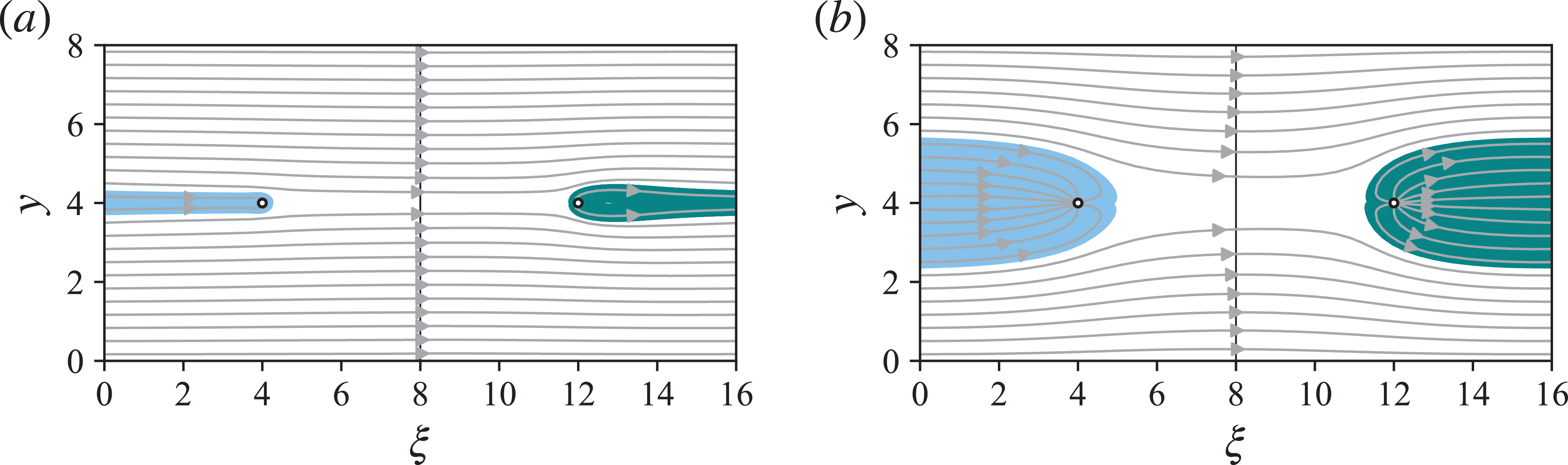
The streamlines of the airflow $\boldsymbol{v}$
are shown in Figure 2 for both purifiers. The flow is broadly unidirectional for the weak purifier (Figure 2
a). Regions in which the streamlines are directed into or out of the purifier are shaded and take up a greater area for the strong purifier (Figure 2
b). In both cases, these regions meet at the periodic boundary.
$\boldsymbol{v}$
are shown in Figure 2 for both purifiers. The flow is broadly unidirectional for the weak purifier (Figure 2
a). Regions in which the streamlines are directed into or out of the purifier are shaded and take up a greater area for the strong purifier (Figure 2
b). In both cases, these regions meet at the periodic boundary.
The airflow streamlines in the $(\xi ,y)$
-plane are shown for (a) the weak purifier (
$(\xi ,y)$
-plane are shown for (a) the weak purifier ( $v_p = 0.04$
) and (b) the strong purifier (
$v_p = 0.04$
) and (b) the strong purifier ( $v_p = 0.3$
). The shaded regions indicate streamlines that pass through the purifier inlet (left) and the purifier outlet (right).
$v_p = 0.3$
). The shaded regions indicate streamlines that pass through the purifier inlet (left) and the purifier outlet (right).
2.5. Terminology: global and local ventilation models
To improve clarity in the discussions below, we here define shorthand labels that refer to the models explored. There are three features that all models compared have in common: (i) the computational domain, which is depicted in Figure 1(b); (ii) the SST solver is used to determine the airflow $\boldsymbol{v}$
; and (iii) the global ventilation rate
$\boldsymbol{v}$
; and (iii) the global ventilation rate $\lambda$
is non-zero.
$\lambda$
is non-zero.
The term global ventilation model here refers to cases in which there are no local ventilation effects. To ensure the computational domain is consistent, the purifier is present but switched off, $v_p = 0$
. This global ventilation model is subtly different to the model of Lau et al. [Reference Lau, Griffiths, English and Kaouri23] due to the existence of the boundaries
$v_p = 0$
. This global ventilation model is subtly different to the model of Lau et al. [Reference Lau, Griffiths, English and Kaouri23] due to the existence of the boundaries $\partial _{\mathrm{in}}$
,
$\partial _{\mathrm{in}}$
, $\partial _{\mathrm{out}}$
and the non-uniform vector field
$\partial _{\mathrm{out}}$
and the non-uniform vector field $\boldsymbol{v}$
. Aside from these minor differences, the underlying modelling assumptions are the same. This model was compared with results reported in Lau et al. [Reference Lau, Griffiths, English and Kaouri23], and the contours of aerosol concentration
$\boldsymbol{v}$
. Aside from these minor differences, the underlying modelling assumptions are the same. This model was compared with results reported in Lau et al. [Reference Lau, Griffiths, English and Kaouri23], and the contours of aerosol concentration $C$
were found to be virtually indistinguishable except in small regions near to the switched-off purifier where differences remained minimal.
$C$
were found to be virtually indistinguishable except in small regions near to the switched-off purifier where differences remained minimal.
We consider three global ventilation levels, which will be referred to by the ACH: The control case 0.7 ACH, in which the only ventilation is provided by the ineffective AC unit; 1.4 ACH, equivalent to the total air exchange rate for the weak purifier; and 6 ACH, equivalent to the total air exchange rate for the strong purifier.
The term local ventilation model refers to the cases in which the purifier is switched on, i.e. $v_p \neq 0$
. In these cases, the global ventilation rate is that of the control case, 0.7 ACH, so we are considering the combined ventilation of the ineffective AC unit (treated globally) and the purifier (treated locally). The two local ventilation cases explored are referred to by the purifier strength: The weak purifier (CADR of 140 m
$v_p \neq 0$
. In these cases, the global ventilation rate is that of the control case, 0.7 ACH, so we are considering the combined ventilation of the ineffective AC unit (treated globally) and the purifier (treated locally). The two local ventilation cases explored are referred to by the purifier strength: The weak purifier (CADR of 140 m $^3$
h
$^3$
h $^{-1}$
) and the strong purifier (CADR of 1,000 m
$^{-1}$
) and the strong purifier (CADR of 1,000 m $^3$
h
$^3$
h $^{-1}$
).
$^{-1}$
).
2.6. Computational speed
The model was solved in COMSOL Multiphysics $^{\circledR }$
on a triangular mesh using the predefined ‘Finer’ mesh, with a maximum element size of
$^{\circledR }$
on a triangular mesh using the predefined ‘Finer’ mesh, with a maximum element size of $0.224$
m. The automatic ‘Fluid dynamics’ calibration resolved the boundary layers with smaller elements near to boundaries. The point source was approximated by uniform production within a small circle, radius
$0.224$
m. The automatic ‘Fluid dynamics’ calibration resolved the boundary layers with smaller elements near to boundaries. The point source was approximated by uniform production within a small circle, radius $r_s = 2.5$
mm. Consequently, a finer mesh was produced around
$r_s = 2.5$
mm. Consequently, a finer mesh was produced around $\boldsymbol{x}_0 = (x_0, y_0)$
. To ensure the symmetry of the problem was numerically realisable, a symmetric mesh about the centreline
$\boldsymbol{x}_0 = (x_0, y_0)$
. To ensure the symmetry of the problem was numerically realisable, a symmetric mesh about the centreline $y_0 = L_y/2$
was used. For scenarios in which
$y_0 = L_y/2$
was used. For scenarios in which $y_0 \neq L_y/2$
, this resulted in an additional region of finer meshing near
$y_0 \neq L_y/2$
, this resulted in an additional region of finer meshing near $(x_0, L_y - y_0)$
, resulting in slightly more mesh elements than when
$(x_0, L_y - y_0)$
, resulting in slightly more mesh elements than when $y_0 = L_y/2$
. Each mesh contained approximately
$y_0 = L_y/2$
. Each mesh contained approximately $21,000$
nodes (though the precise number differed for each
$21,000$
nodes (though the precise number differed for each $\boldsymbol{x}_0$
). Both the flow field and the ADR equation were solved on the same mesh.
$\boldsymbol{x}_0$
). Both the flow field and the ADR equation were solved on the same mesh.
The mesh independency was explored as follows: all parameters were fixed, and the problem (both airflow and ADR equation) was solved using the automatic resolution settings ranging from ‘Coarser’ to ‘Extremely Fine’. For direct comparison, each solution was interpolated onto a fine uniform grid (using cubic splines), and the relative error between the ‘Extremely Fine’ mesh (around 90,000 nodes) and each of the other meshes was calculated at each grid point, then integrated over the domain (using Simpson’s rule). The ‘Finer’ mesh ensured a discrepancy of the order of $10^{-3}$
and resulted in plots that were visually indistinguishable from those for the ‘Extremely Fine’ mesh.
$10^{-3}$
and resulted in plots that were visually indistinguishable from those for the ‘Extremely Fine’ mesh.
Simulations were performed on a Lenovo IdeaPad Flex 5 laptop, with a 1.3 GHz 4-core Intel Core i7-1065G7 processor and 8 GB of RAM. For each airflow simulation (switched-off purifier, weak purifier and strong purifier) to reach a steady state, computation takes approximately 10 minutes. For the ADR equation (2.4), an event lasting 4 hours takes around 5 minutes to run, including calculation of the infection risk (2.9). At these computational speeds, advice and guidance can be quickly updated with new information during a fast-changing epidemic.
3. Average aerosol concentration
We define the average aerosol concentration in the room as
 \begin{equation} \bar {C}(t) = \frac {1}{V} \iint _{\Omega } \mathscr{C}\kern1pt(\xi ,y,t) \, \mathrm{d} \xi \, \mathrm{d} y, \end{equation}
where $\Omega$
denotes the computational domain depicted in Figure 1(b). Taking appropriate integrals of (2.4), the divergence theorem is applied to the advective and diffusive terms, giving
$\Omega$
denotes the computational domain depicted in Figure 1(b). Taking appropriate integrals of (2.4), the divergence theorem is applied to the advective and diffusive terms, giving
 \begin{equation} \frac {\partial \bar {C}}{\partial t} = \frac {R}{V} - (\lambda + \beta + \sigma ) \bar {C} - \frac {1}{V} \oint _{\partial _{\mathrm{in}}} v_p \mathscr{C} \, \mathrm{d} l, \end{equation}
where $l$
denotes a line element on
$l$
denotes a line element on $\partial _{\mathrm{in}}$
. When
$\partial _{\mathrm{in}}$
. When $v_p \neq 0$
, the boundary integral (describing aerosol removal by the purifier) depends on the values of
$v_p \neq 0$
, the boundary integral (describing aerosol removal by the purifier) depends on the values of $\mathscr{C}$
on the purifier inlet boundary
$\mathscr{C}$
on the purifier inlet boundary $\partial _{\mathrm{in}}$
(2.3), which depend on the distribution of aerosols around the room. Hence,
$\partial _{\mathrm{in}}$
(2.3), which depend on the distribution of aerosols around the room. Hence, $\bar {C}$
implicitly depends on the location of the infectious source
$\bar {C}$
implicitly depends on the location of the infectious source $\boldsymbol{x}_0$
and the strength of the purifier. When
$\boldsymbol{x}_0$
and the strength of the purifier. When $v_p = 0$
, there is no local ventilation (as in Lau et al. [Reference Lau, Griffiths, English and Kaouri23]), the boundary integral vanishes and (3.2) is equivalent to the Wells–Riley model (2.1). In this case, the solution to (3.2) is given by
$v_p = 0$
, there is no local ventilation (as in Lau et al. [Reference Lau, Griffiths, English and Kaouri23]), the boundary integral vanishes and (3.2) is equivalent to the Wells–Riley model (2.1). In this case, the solution to (3.2) is given by
 \begin{equation} \bar {C}(t) = C^* \left [1 - \mathrm{e}^{-(\lambda +\beta +\sigma )t} \right ], \; \; \mathrm{where} \; \; C^* = \frac {R}{(\lambda +\beta +\sigma )V}. \end{equation}
Hence, $\bar {C}$
does not depend on
$\bar {C}$
does not depend on $\boldsymbol{x}_0$
or
$\boldsymbol{x}_0$
or $\boldsymbol{v}$
for the global ventilation cases, and
$\boldsymbol{v}$
for the global ventilation cases, and $\bar {C} \rightarrow C^*$
as
$\bar {C} \rightarrow C^*$
as $t \rightarrow \infty$
.
$t \rightarrow \infty$
.
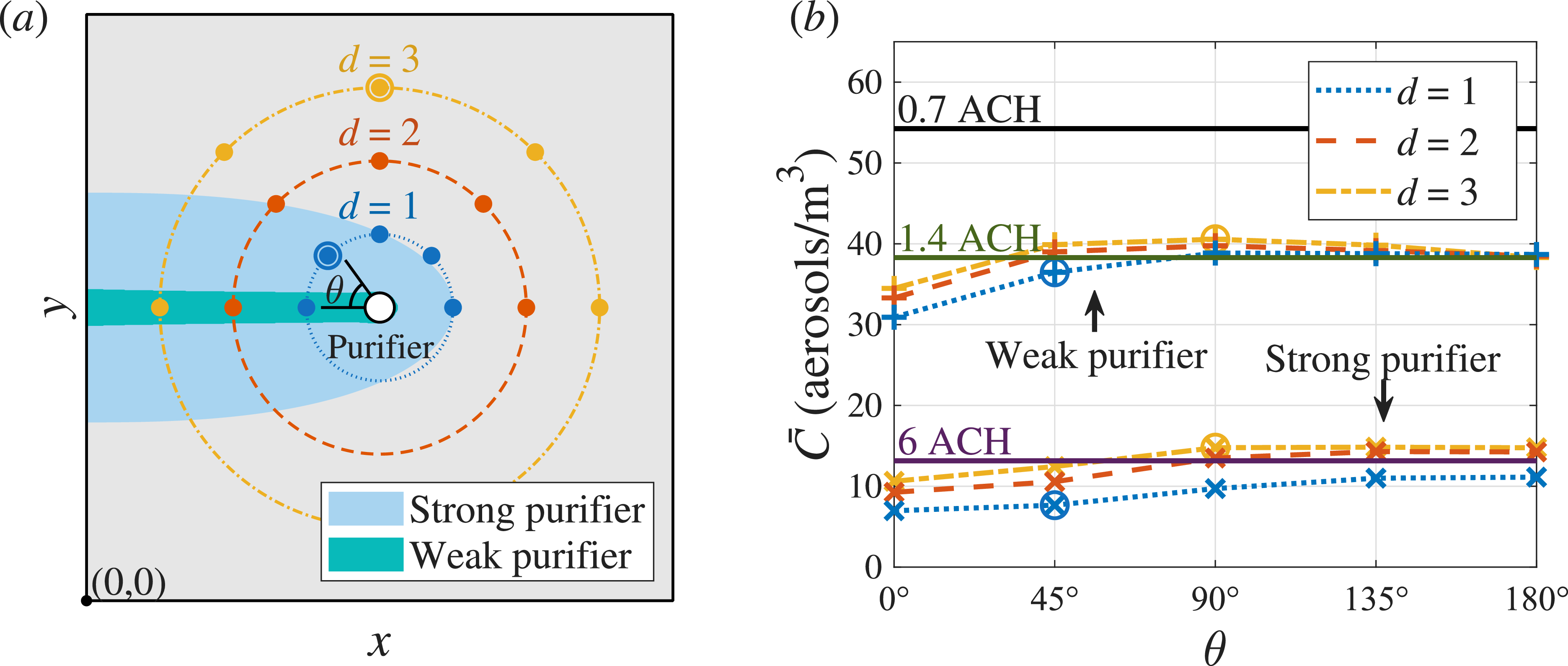
In (a), the infectious source locations, $\boldsymbol{x}_0$
, are depicted by filled circles and the regions where all streamlines are directed into the purifier inlet (Figure 2) are shaded for each purifier. In (b), the average aerosol concentration,
$\boldsymbol{x}_0$
, are depicted by filled circles and the regions where all streamlines are directed into the purifier inlet (Figure 2) are shaded for each purifier. In (b), the average aerosol concentration, $\bar {C}$
, after 4 hours is shown for the weak (
$\bar {C}$
, after 4 hours is shown for the weak ( $+$
) and the strong (
$+$
) and the strong ( $\times$
) purifiers for these
$\times$
) purifiers for these $\boldsymbol{x}_0$
. The global ventilation cases are also shown in (b), depicted as horizontal lines (labelled with the ACH). The cases explored further in Figures 4 and 5 are indicated with circles.
$\boldsymbol{x}_0$
. The global ventilation cases are also shown in (b), depicted as horizontal lines (labelled with the ACH). The cases explored further in Figures 4 and 5 are indicated with circles.
We express the location of the infectious source relative to the purifier location as
 \begin{equation} \boldsymbol{x}_0 = (x_0,y_0) = (x_p - d \, \mathrm{cos} \, \theta , y_p + d \, \mathrm{sin} \, \theta ), \end{equation}
where $d$
is the distance from the purifier and
$d$
is the distance from the purifier and $\theta$
is the angle (in degrees) from the line
$\theta$
is the angle (in degrees) from the line $y = L_y/2$
. The problem is symmetric in this line so we consider only
$y = L_y/2$
. The problem is symmetric in this line so we consider only $\theta \in [0^{\circ },180^{\circ }]$
. In Figure 3(a), we show all choices of
$\theta \in [0^{\circ },180^{\circ }]$
. In Figure 3(a), we show all choices of $(d,\theta )$
considered here.
$(d,\theta )$
considered here.
To compare the long-time behaviour of the different ventilation models, $\bar {C}$
is plotted in Figure 3(b) after an event of 4 hours. This duration is representative of certain social settings (e.g. restaurants), activities within all-day events (such as conferences, workshops and networking events) and time spent working in open-plan offices. For all the cases considered here,
$\bar {C}$
is plotted in Figure 3(b) after an event of 4 hours. This duration is representative of certain social settings (e.g. restaurants), activities within all-day events (such as conferences, workshops and networking events) and time spent working in open-plan offices. For all the cases considered here, $\mathscr{C}$
reaches a steady state within this time.
$\mathscr{C}$
reaches a steady state within this time.
For the global ventilation models, $\bar {C} = C^*$
(3.3), which we evaluate for 0.7 ACH, 1.4 ACH and 6 ACH; plotted as horizontal lines in Figure 3(b). There is good agreement between each purifier and the equivalent global ventilation for most
$\bar {C} = C^*$
(3.3), which we evaluate for 0.7 ACH, 1.4 ACH and 6 ACH; plotted as horizontal lines in Figure 3(b). There is good agreement between each purifier and the equivalent global ventilation for most $(d,\theta )$
choices. For the weak purifier, the only significant deviation is when
$(d,\theta )$
choices. For the weak purifier, the only significant deviation is when $\theta = 0$
(for all values of
$\theta = 0$
(for all values of $d$
). For the strong purifier, the discrepancy is significant for
$d$
). For the strong purifier, the discrepancy is significant for $d = 1$
(for all values of
$d = 1$
(for all values of $\theta$
) and for small
$\theta$
) and for small $\theta$
when
$\theta$
when $d = 2,3$
. Where the results differ the most, the global ventilation overestimates
$d = 2,3$
. Where the results differ the most, the global ventilation overestimates $\bar {C}$
compared to the local purifier model. When
$\bar {C}$
compared to the local purifier model. When $d = 2, 3$
, the global ventilation model underestimates
$d = 2, 3$
, the global ventilation model underestimates $\bar {C}$
for some
$\bar {C}$
for some $\theta$
, but the discrepancy is relatively small.
$\theta$
, but the discrepancy is relatively small.
In Figure 3(b), we show that $\bar {C}$
increases with
$\bar {C}$
increases with $d$
for both purifiers; purifiers are less effective when the infectious person is further away. This aligns with the intuitive expectation that placing the infectious source nearer to the purifier would allow the purifier to capture a greater number of aerosols, hence reducing the average concentration,
$d$
for both purifiers; purifiers are less effective when the infectious person is further away. This aligns with the intuitive expectation that placing the infectious source nearer to the purifier would allow the purifier to capture a greater number of aerosols, hence reducing the average concentration, $\bar {C}$
. Also, both purifiers are more effective (with
$\bar {C}$
. Also, both purifiers are more effective (with $\bar {C}$
decreasing) when the infectious person is located in the shaded region where all streamlines enter the purifier inlet. In these cases, the global ventilation overestimates the concentration. When
$\bar {C}$
decreasing) when the infectious person is located in the shaded region where all streamlines enter the purifier inlet. In these cases, the global ventilation overestimates the concentration. When $\boldsymbol{x}_0$
is outside of these regions, there is less variation in
$\boldsymbol{x}_0$
is outside of these regions, there is less variation in $\bar {C}$
and closer agreement between the ventilation models.
$\bar {C}$
and closer agreement between the ventilation models.
Contour plots of the aerosol concentration $C$
after 4 hours for an infectious source at
$C$
after 4 hours for an infectious source at $\boldsymbol{x}_0$
(3.4) with
$\boldsymbol{x}_0$
(3.4) with $(d,\theta ) = (1,45^{\circ })$
(see Figure 3a). The concentration is shown for (a) the weak purifier (
$(d,\theta ) = (1,45^{\circ })$
(see Figure 3a). The concentration is shown for (a) the weak purifier ( $C_p$
) and (b) the equivalent global ventilation of 1.4 ACH (
$C_p$
) and (b) the equivalent global ventilation of 1.4 ACH ( $C_g$
), both with contours at intervals of 10 aerosols/m
$C_g$
), both with contours at intervals of 10 aerosols/m $^3$
. The concentration is shown for (c) the strong purifier (
$^3$
. The concentration is shown for (c) the strong purifier ( $C_p$
) and (d) the equivalent global ventilation of 6 ACH (
$C_p$
) and (d) the equivalent global ventilation of 6 ACH ( $C_g$
), both with contours at intervals of 3 aerosols/m
$C_g$
), both with contours at intervals of 3 aerosols/m $^3$
.
$^3$
.
4. Spatial distribution of aerosols
The spatiotemporal model also provides information on the spatial distribution of aerosols around the room. The local and global ventilation models were compared for the infectious source locations depicted in Figure 3(a). Contour plots showing the spatial variation of $C$
after 4 hours (as in Figure 3) are given in Figures 4 and 5 for some representative examples. For this discussion, we will denote the concentration for the local ventilation model (purifier) by
$C$
after 4 hours (as in Figure 3) are given in Figures 4 and 5 for some representative examples. For this discussion, we will denote the concentration for the local ventilation model (purifier) by $C_p$
and for the equivalent global ventilation model by
$C_p$
and for the equivalent global ventilation model by $C_g$
.
$C_g$
.
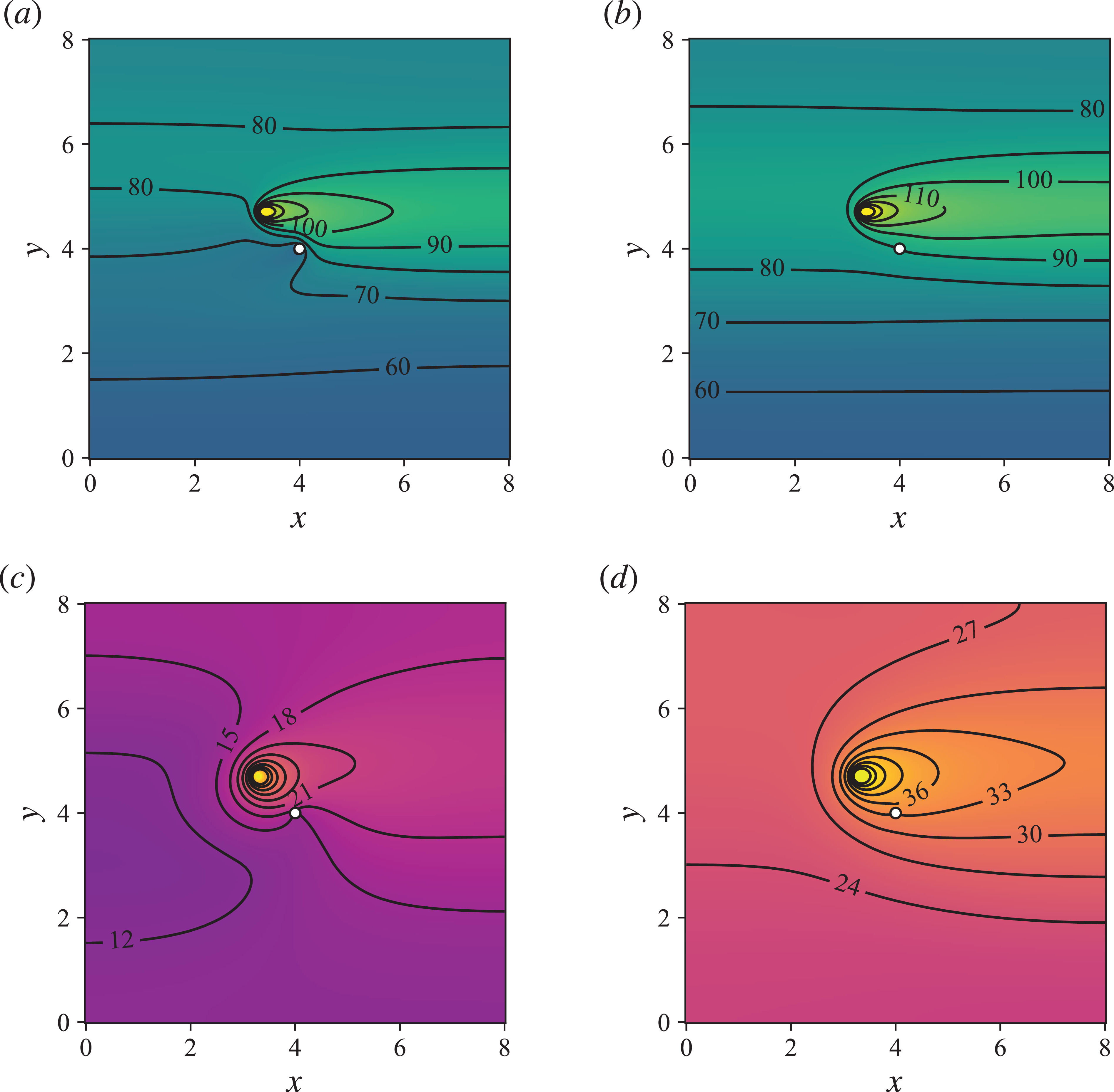
The concentration around the room is shown in Figure 4 when $(d,\theta ) = (1,45^{\circ })$
for both purifiers and the equivalent global ventilations. In Figure 4(a,b),
$(d,\theta ) = (1,45^{\circ })$
for both purifiers and the equivalent global ventilations. In Figure 4(a,b), $C_p$
and
$C_p$
and $C_g$
are shown (respectively) for the weak purifier. There is a similar concentration throughout the room for both ventilation models, but
$C_g$
are shown (respectively) for the weak purifier. There is a similar concentration throughout the room for both ventilation models, but $C_p \lt C_g$
everywhere. The largest discrepancies are below and to the left of the purifier and to the right of the infectious source. Similar features were observed for all cases in which the infectious source is located near to (but outside of) the region where streamlines are directed into the purifier inlet (Figure 3a).
$C_p \lt C_g$
everywhere. The largest discrepancies are below and to the left of the purifier and to the right of the infectious source. Similar features were observed for all cases in which the infectious source is located near to (but outside of) the region where streamlines are directed into the purifier inlet (Figure 3a).
Contour plots of the aerosol concentration $C$
after 4 hours for an infectious source at
$C$
after 4 hours for an infectious source at $\boldsymbol{x}_0$
(3.4) with
$\boldsymbol{x}_0$
(3.4) with $(d,\theta ) = (3,90^{\circ })$
(see Figure 3a). The concentration is shown for (a) the weak purifier (
$(d,\theta ) = (3,90^{\circ })$
(see Figure 3a). The concentration is shown for (a) the weak purifier ( $C_p$
) and (b) the equivalent global ventilation of 1.4 ACH (
$C_p$
) and (b) the equivalent global ventilation of 1.4 ACH ( $C_g$
), both with contours at intervals of 14 aerosols/m
$C_g$
), both with contours at intervals of 14 aerosols/m $^3$
. The concentration is shown for (c) the strong purifier (
$^3$
. The concentration is shown for (c) the strong purifier ( $C_p$
) and (d) the equivalent global ventilation of 6 ACH (
$C_p$
) and (d) the equivalent global ventilation of 6 ACH ( $C_g$
), both with contours at intervals of 5 aerosols/m
$C_g$
), both with contours at intervals of 5 aerosols/m $^3$
. Additional dashed lines show where
$^3$
. Additional dashed lines show where $C_p = C_g$
.
$C_p = C_g$
.
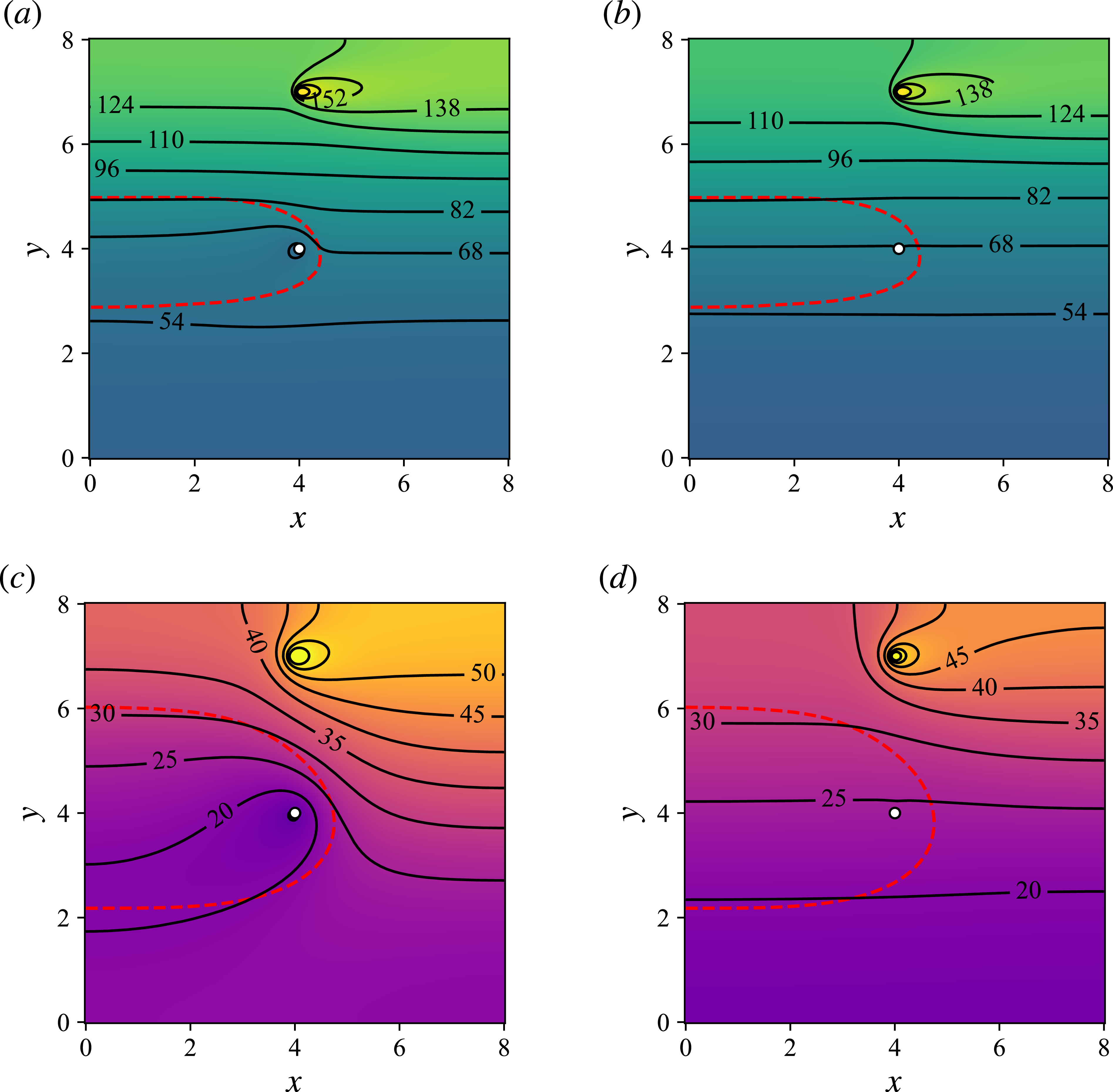
Figure 4(c,d) shows $C_p, C_g$
(respectively) for the strong purifier. In this case, the global ventilation model significantly overestimates the concentration compared to the local ventilation model. For instance,
$C_p, C_g$
(respectively) for the strong purifier. In this case, the global ventilation model significantly overestimates the concentration compared to the local ventilation model. For instance, $C_g \gt 21$
aerosols/m
$C_g \gt 21$
aerosols/m $^3$
everywhere in Figure 4(d), whereas
$^3$
everywhere in Figure 4(d), whereas $C_p \lt 21$
aerosols/m
$C_p \lt 21$
aerosols/m $^3$
in the majority of the room in Figure 4(c). These observations are indicative of all cases where the infectious source lies inside the region where streamlines are directed into the purifier inlet (see Figure 3a).
$^3$
in the majority of the room in Figure 4(c). These observations are indicative of all cases where the infectious source lies inside the region where streamlines are directed into the purifier inlet (see Figure 3a).
In Figure 5, we consider the distribution of aerosols when $(d,\theta ) = (3,90^{\circ })$
. These are representative examples for the cases where the infectious source is far away from the region where the streamlines are directed into the purifier inlet.
$(d,\theta ) = (3,90^{\circ })$
. These are representative examples for the cases where the infectious source is far away from the region where the streamlines are directed into the purifier inlet.
Comparing $C_p$
and
$C_p$
and $C_g$
for the weak purifier (Figures 5a,b), the concentration is similar throughout the room, except for the region
$C_g$
for the weak purifier (Figures 5a,b), the concentration is similar throughout the room, except for the region $y \gt 5$
, where
$y \gt 5$
, where $C_p$
is approximately one contour level (14 aerosols/m
$C_p$
is approximately one contour level (14 aerosols/m $^3$
) larger than
$^3$
) larger than $C_g$
. There are regions in the room where
$C_g$
. There are regions in the room where $C_p \lt C_g$
(near the purifier) and where
$C_p \lt C_g$
(near the purifier) and where $C_p \gt C_g$
(near the infectious source), with the dashed red line (the same in both plots) showing the boundary between these regions, i.e. where
$C_p \gt C_g$
(near the infectious source), with the dashed red line (the same in both plots) showing the boundary between these regions, i.e. where $C_p = C_g$
(no such lines appear in Figure 4 since
$C_p = C_g$
(no such lines appear in Figure 4 since $C_p \lt C_g$
everywhere in those cases).
$C_p \lt C_g$
everywhere in those cases).
For the strong purifier example shown in Figure 5(c,d), the spatial distribution of aerosols differs more significantly between the ventilation models. The region where $C_p \lt C_g$
is larger in this case, but where
$C_p \lt C_g$
is larger in this case, but where $C_p \gt C_g$
the concentration difference ranges from around 1 contour level (5 aerosols/m
$C_p \gt C_g$
the concentration difference ranges from around 1 contour level (5 aerosols/m $^3$
), in the top left and bottom right of the room, to around 2 contour levels, in the top right (near to the infectious source). This suggests that the global ventilation model better captures the aerosol distribution of the weak purifier than the strong purifier.
$^3$
), in the top left and bottom right of the room, to around 2 contour levels, in the top right (near to the infectious source). This suggests that the global ventilation model better captures the aerosol distribution of the weak purifier than the strong purifier.
5. Infection risk to susceptible people
Our spatially varying model allows us to determine the infection risk to susceptible people at specific locations (2.9). We express the location of a susceptible person $\boldsymbol{x}_s$
as
$\boldsymbol{x}_s$
as
 \begin{equation} \boldsymbol{x}_s = (x_s,y_s) = (x_p - d_s \, \mathrm{cos} (\theta + \phi ), y_p + d_s \, \mathrm{sin}(\theta + \phi )), \end{equation}
where $\phi$
is the angle between
$\phi$
is the angle between $\boldsymbol{x}_0$
and
$\boldsymbol{x}_0$
and $\boldsymbol{x}_s$
, and
$\boldsymbol{x}_s$
, and $d_s$
is the distance from the purifier.
$d_s$
is the distance from the purifier.
The infection risk, $P$
(equation (2.9)), to the susceptible person at
$P$
(equation (2.9)), to the susceptible person at $\boldsymbol{x}_s$
(see (5.1)) after 1 hour with (a)
$\boldsymbol{x}_s$
(see (5.1)) after 1 hour with (a) $\phi = 180^{\circ }$
and (b)
$\phi = 180^{\circ }$
and (b) $\phi = 90^{\circ }$
. Global ventilation cases are labelled with their ACH value (open symbols), and the equivalent local ventilation (purifier) is depicted by filled symbols of the same shape. Schematics in the lower axes show the locations of the infectious and susceptible people for each
$\phi = 90^{\circ }$
. Global ventilation cases are labelled with their ACH value (open symbols), and the equivalent local ventilation (purifier) is depicted by filled symbols of the same shape. Schematics in the lower axes show the locations of the infectious and susceptible people for each $\theta$
.
$\theta$
.
To reflect a scenario in which the susceptible and infectious individuals are in close proximity, we consider $d = d_s = 1$
(note that
$d = d_s = 1$
(note that $d = 1$
is the case with the greatest discrepancy between the local and global ventilation models in Figure 3). This is reflective of classrooms, lectures and meetings, with 1 hour being a representative event duration. However, in reality, the strong purifier is potentially too large and noisy for use in such a setting.
$d = 1$
is the case with the greatest discrepancy between the local and global ventilation models in Figure 3). This is reflective of classrooms, lectures and meetings, with 1 hour being a representative event duration. However, in reality, the strong purifier is potentially too large and noisy for use in such a setting.
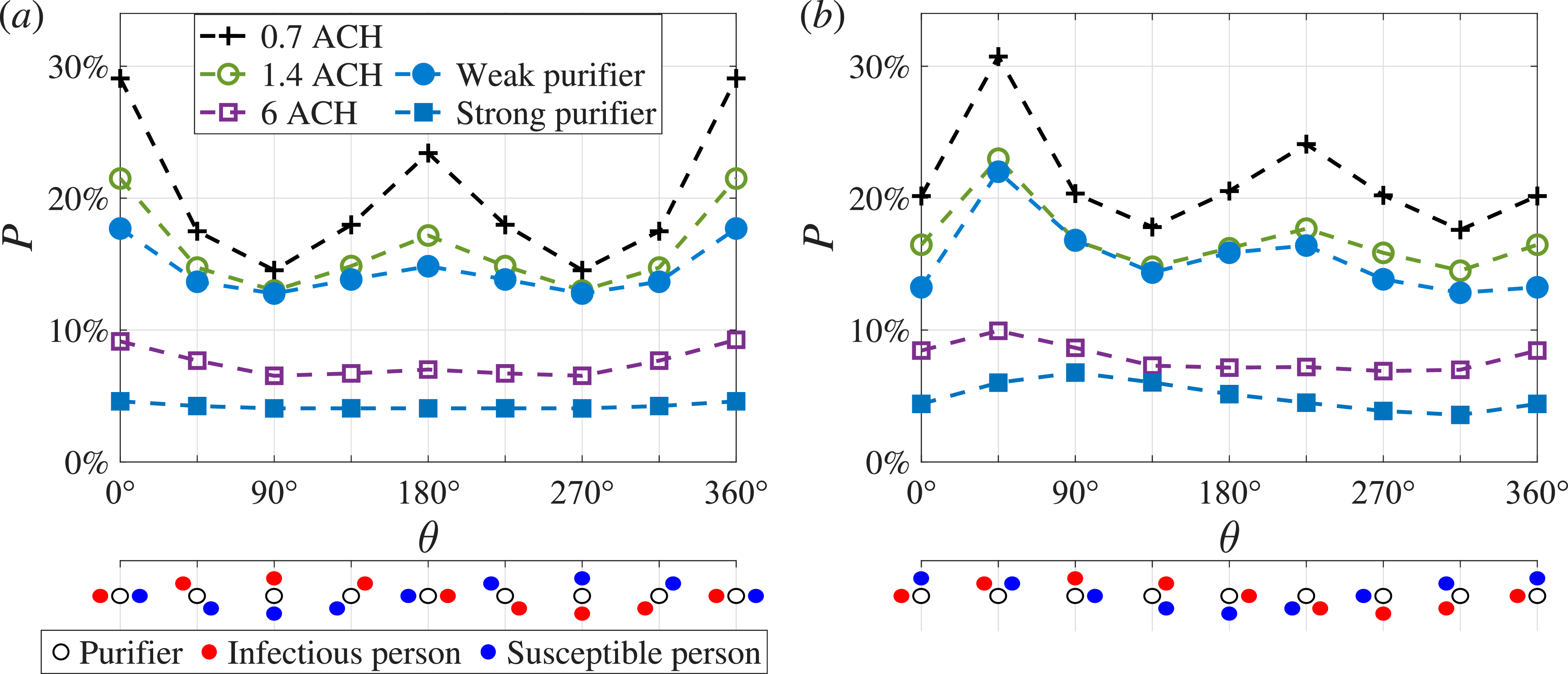
Two configurations of the susceptible and infectious people are considered: (i) they are opposite each other with the purifier in between them, $\phi = 180^{\circ }$
(Figure 6a) and (ii) they are to one side of the purifier,
$\phi = 180^{\circ }$
(Figure 6a) and (ii) they are to one side of the purifier, $\phi = 90^{\circ }$
(Figure 6b). Figure 6 shows the infection risk to the susceptible person after 1 hour, with the scenario for each
$\phi = 90^{\circ }$
(Figure 6b). Figure 6 shows the infection risk to the susceptible person after 1 hour, with the scenario for each $\theta$
depicted on the lower axes. In Figure 6(a),
$\theta$
depicted on the lower axes. In Figure 6(a), $P$
is symmetric around
$P$
is symmetric around $\theta = 180^{\circ }$
because both the ADR equation and the airflow are symmetric in the line
$\theta = 180^{\circ }$
because both the ADR equation and the airflow are symmetric in the line $y = L_y/2$
. Moreover, the case
$y = L_y/2$
. Moreover, the case $\phi = - 90^{\circ }$
can be deduced from Figure 6(b) by reflection in this line (
$\phi = - 90^{\circ }$
can be deduced from Figure 6(b) by reflection in this line ( $\theta \rightarrow 360^{\circ } - \theta$
).
$\theta \rightarrow 360^{\circ } - \theta$
).
After 1 hour, the infection risk is below 40% in all cases, and the global ventilation model overestimates the infection risk. The weak purifier has had only a marginal effect when compared against the baseline example of 0.7 ACH and shows close agreement with the corresponding global ventilation of 1.4 ACH. The infection risk is lower for the strong purifier than for the equivalent global ventilation of 6 ACH for all values of $\theta$
. The greatest discrepancy is when
$\theta$
. The greatest discrepancy is when $\theta = 0^{\circ }$
, with the strong purifier predicting half the infection risk of the 6 ACH global ventilation (Figure 6a,b).
$\theta = 0^{\circ }$
, with the strong purifier predicting half the infection risk of the 6 ACH global ventilation (Figure 6a,b).
The streamlines of $\boldsymbol{v}$
again provide insight into these results. For the global ventilation models and the weak purifier, peaks occur when
$\boldsymbol{v}$
again provide insight into these results. For the global ventilation models and the weak purifier, peaks occur when $y_0 = y_s$
due to the broadly unidirectional flow around the recirculating loop, with lower peaks when the aerosols travel further (e.g.
$y_0 = y_s$
due to the broadly unidirectional flow around the recirculating loop, with lower peaks when the aerosols travel further (e.g. $\theta = 180^{\circ }$
in Figure 6a). For the strong purifier, the largest infection risk (
$\theta = 180^{\circ }$
in Figure 6a). For the strong purifier, the largest infection risk ( $\theta = 90^{\circ }$
in Figure 6b) corresponds to the susceptible person being directly downstream from the infectious person according to the significantly modified streamlines in this case (Figure 2b).
$\theta = 90^{\circ }$
in Figure 6b) corresponds to the susceptible person being directly downstream from the infectious person according to the significantly modified streamlines in this case (Figure 2b).
Under the well-mixed-room assumption, the infection risk is calculated based on the average aerosol concentration, $\bar {C}$
(3.3). This approach predicts the following infection risks: 8.8% for 0.7 ACH, 7.5% for 1.4 ACH and 3.6% for 6 ACH. This is a significant underestimate compared to the corresponding values in Figure 6 since the proximity to the infectious source results in a concentration significantly greater than the room average at all times.
$\bar {C}$
(3.3). This approach predicts the following infection risks: 8.8% for 0.7 ACH, 7.5% for 1.4 ACH and 3.6% for 6 ACH. This is a significant underestimate compared to the corresponding values in Figure 6 since the proximity to the infectious source results in a concentration significantly greater than the room average at all times.
6. Summary and conclusions
Motivated by air purifiers, the spatiotemporal modelling framework of Lau et al. [Reference Lau, Griffiths, English and Kaouri23] for airborne disease transmission was modified to incorporate local ventilation effects. For a weak purifier (CADR = 140 m $^3$
h
$^3$
h $^{-1}$
) and a strong purifier (CADR = 1,000 m
$^{-1}$
) and a strong purifier (CADR = 1,000 m $^3$
h
$^3$
h $^{-1}$
), the local ventilation model introduced here was compared against a global ventilation model (consistent with Lau et al. [Reference Lau, Griffiths, English and Kaouri23]), with 1.4 ACH and 6 ACH, respectively.
$^{-1}$
), the local ventilation model introduced here was compared against a global ventilation model (consistent with Lau et al. [Reference Lau, Griffiths, English and Kaouri23]), with 1.4 ACH and 6 ACH, respectively.
For each purifier, the average aerosol concentration $\bar {C}$
, after reaching a steady state, was compared for the local and global ventilation models, with good agreement in most cases (Figure 3). For the local ventilation model,
$\bar {C}$
, after reaching a steady state, was compared for the local and global ventilation models, with good agreement in most cases (Figure 3). For the local ventilation model, $\bar {C}$
depends on the infectious source location and increasing the distance between the infectious person and the purifier increases the average concentration. The lowest values of
$\bar {C}$
depends on the infectious source location and increasing the distance between the infectious person and the purifier increases the average concentration. The lowest values of $\bar {C}$
were observed when the infectious source is inside the regions where the airflow streamlines are directed into the purifier inlet (Figure 2). When the infectious source is inside these regions, the global ventilation model significantly overestimates
$\bar {C}$
were observed when the infectious source is inside the regions where the airflow streamlines are directed into the purifier inlet (Figure 2). When the infectious source is inside these regions, the global ventilation model significantly overestimates $\bar {C}$
. When the infectious source is located outside of these regions, there is better agreement between the two ventilation models, particularly for the weak purifier.
$\bar {C}$
. When the infectious source is located outside of these regions, there is better agreement between the two ventilation models, particularly for the weak purifier.
When the infectious person is located inside or near to these regions, the global ventilation model overestimates the aerosol concentration everywhere in the room (Figure 4). However, when the infectious source is far from the purifier, there are some regions where the global ventilation model predicts larger concentrations, and other regions where it predicts lower concentrations than the local ventilation model (Figure 5). In these cases, the agreement between the local and global ventilation models is better for the weak purifier.
The infection risk to susceptible people near the purifier after one hour was also considered (Figure 6). The weak purifier showed good agreement with the global ventilation model, whereas the strong purifier predicts a lower infection risk than the equivalent global ventilation (Figure 6). The largest discrepancies between the local and global ventilation models were observed when the susceptible person was located directly downstream from the infectious person according to the modified airflow streamlines (Figure 2). The global ventilation model overestimates infection risk compared to the local ventilation model in these cases.
When modelling airborne transmission, Wells–Riley models (e.g. Miller [Reference Miller28]) offer very high computational speeds but are very simple, whereas CFD models, particularly those that track individual particles (e.g. Dbouk et al. [Reference Dbouk, Roger and Drikakis11]), provide significant detail at much greater computational cost. The modelling framework of Lau et al. [Reference Lau, Griffiths, English and Kaouri23] offers a compromise between these models, including spatial variation at low computational cost. Here, we increased the complexity by developing a model incorporating local ventilation over hours, the time frame over which airborne transmission occurs, while still retaining relatively small computational times; around five minutes of simulation time for 4-hour events.
In future, these fast simulations could allow a more thorough investigation, exploring factors such as purifier location, size and strength. The model could be further developed by incorporating a spatially varying eddy diffusion coefficient or the unsteady airflow produced when the purifier is switched on at a given time. The local ventilation effects of AC, windows, doors and other purifier designs could also be explored, with the caveat that such features may promote interaction between the recirculation layers, and hence undermine this underlying assumption. Experimental studies and CFD would provide insight into when the recirculating flow assumption is valid. Even in cases where this assumption breaks down, the rationale of using a simplified airflow to produce fast predictions could still be applied to explore different AC unit designs, different purifier designs and other types of ventilation, provided an appropriate simplified airflow can be determined.
Acknowledgements
The authors wish to acknowledge the contributions of Dr. Aaron English, Dr. Raquel González Fariña and Dr. Attila Kovács. We are grateful to Siân Grant for generating Figure 1(a).
Funding statement
A.P. and K.K. gratefully acknowledge funding from a Sêr Cymru ‘Tackling COVID-19’ grant, awarded by the Welsh Government. I.M.G. is grateful to the Royal Society for funding through a University Research Fellowship.
Competing interests
The authors report no conflict of interest.
Appendix A. Turbulent flow solver
A.1. Reynolds-averaged Navier–Stokes equations
Consider the Navier–Stokes equations
 \begin{align} \rho \frac {\partial \boldsymbol{u}}{\partial t} + \rho (\boldsymbol{u} \cdot \nabla ) \boldsymbol{u} &= - \nabla p + \nabla \cdot \mu (\nabla \boldsymbol{u} + (\nabla \boldsymbol{u})^T ), \end{align}
 \begin{align} \nabla \cdot \boldsymbol{u} &= 0, \end{align}
where $\boldsymbol{u} = (u_x, u_y)$
is the velocity field,
$\boldsymbol{u} = (u_x, u_y)$
is the velocity field, $p$
is the pressure,
$p$
is the pressure, $\rho$
is the fluid density and
$\rho$
is the fluid density and $\mu$
is the dynamic viscosity. The viscous terms are written in this form as it later highlights the viscosity-like effect of turbulent fluctuations on the flow, but for an incompressible flow with constant viscosity (such as air),
$\mu$
is the dynamic viscosity. The viscous terms are written in this form as it later highlights the viscosity-like effect of turbulent fluctuations on the flow, but for an incompressible flow with constant viscosity (such as air), $\nabla \cdot \mu (\nabla \boldsymbol{u} + (\nabla \boldsymbol{u})^T ) = \mu \nabla ^2 \boldsymbol{u}$
. We consider a 2D velocity field
$\nabla \cdot \mu (\nabla \boldsymbol{u} + (\nabla \boldsymbol{u})^T ) = \mu \nabla ^2 \boldsymbol{u}$
. We consider a 2D velocity field $\boldsymbol{u}$
for the current problem, but generally present equations in vector notation so that the derivation is applicable to 3D flows.
$\boldsymbol{u}$
for the current problem, but generally present equations in vector notation so that the derivation is applicable to 3D flows.
A Reynolds decomposition is applied to the flow variables,
 \begin{equation} \psi = \bar {\psi } + \psi ', \end{equation}
where $\bar {\psi }$
is a time-averaged mean quantity, and
$\bar {\psi }$
is a time-averaged mean quantity, and $\psi '$
represents turbulent fluctuations. This decomposition is applied for all flow variables, i.e.
$\psi '$
represents turbulent fluctuations. This decomposition is applied for all flow variables, i.e. $\psi = u_x, u_y, p$
. For consistency of notation with Section 2, we will refer to the time-averaged vector field
$\psi = u_x, u_y, p$
. For consistency of notation with Section 2, we will refer to the time-averaged vector field $\boldsymbol{\bar {u}}$
as
$\boldsymbol{\bar {u}}$
as $\boldsymbol{v}$
. Applying the decomposition (A.2) to (A.1) and time-averaging the resulting equations (noting that the time-average of fluctuation variables is zero) gives the Reynolds-averaged Navier–Stokes equations (RANS) governing the mean flow
$\boldsymbol{v}$
. Applying the decomposition (A.2) to (A.1) and time-averaging the resulting equations (noting that the time-average of fluctuation variables is zero) gives the Reynolds-averaged Navier–Stokes equations (RANS) governing the mean flow
 \begin{align*} \rho \frac {\partial \boldsymbol{v}}{\partial t} + \rho (\boldsymbol{v} \cdot \nabla ) \boldsymbol{v} + \rho \overline {(\boldsymbol{u'} \cdot \nabla ) \boldsymbol{u'}} &= - \nabla \bar {p} + \nabla \cdot \mu (\nabla \boldsymbol{v} + (\nabla \boldsymbol{v})^T ), \\ \nabla \cdot \boldsymbol{v} &= 0, \end{align*}
where all the fluctuation terms vanish due to the time-averaging, except for the one remaining non-linear term. This term can be rewritten in terms of the Reynolds stress $\mathcal{R} = \rho \overline {(\boldsymbol{u'} \otimes \boldsymbol{u'})}$
:
$\mathcal{R} = \rho \overline {(\boldsymbol{u'} \otimes \boldsymbol{u'})}$
:
 \begin{equation*} \rho \overline {(\boldsymbol{u'} \cdot \nabla ) \boldsymbol{u'}} = \nabla \cdot \mathcal{R}, \end{equation*}
where the divergence operator is applied row-wise to the tensor $\mathcal{R}$
. Note that this equivalence holds only for incompressible flows since in general we have
$\mathcal{R}$
. Note that this equivalence holds only for incompressible flows since in general we have $\nabla \cdot (\boldsymbol{a} \otimes \boldsymbol{a}) = ( \boldsymbol{a} \cdot \nabla ) \boldsymbol{a} + \boldsymbol{a} \cdot (\nabla \cdot \boldsymbol{a})$
for any vector field
$\nabla \cdot (\boldsymbol{a} \otimes \boldsymbol{a}) = ( \boldsymbol{a} \cdot \nabla ) \boldsymbol{a} + \boldsymbol{a} \cdot (\nabla \cdot \boldsymbol{a})$
for any vector field $\boldsymbol{a}$
.
$\boldsymbol{a}$
.
The term $\nabla \cdot \mathcal{R}$
represents the stress-like effect that turbulent fluctuations have on the mean flow. Following the Boussinesq approach, we assume that turbulence is of a purely diffusive nature, in which case the Reynolds stress can be written as
$\nabla \cdot \mathcal{R}$
represents the stress-like effect that turbulent fluctuations have on the mean flow. Following the Boussinesq approach, we assume that turbulence is of a purely diffusive nature, in which case the Reynolds stress can be written as
 \begin{equation*} \mathcal{R} = \frac {2}{3} \rho k - \mu _T (\nabla \boldsymbol{v} + (\nabla \boldsymbol{v})^T ), \end{equation*}
where $k = \frac {1}{2} (u_x^2 + u_y^2)$
is the turbulent kinetic energy and
$k = \frac {1}{2} (u_x^2 + u_y^2)$
is the turbulent kinetic energy and $\mu _T$
is the eddy viscosity (or turbulent viscosity) of the flow. Both of these quantities are, in general, spatially dependent.
$\mu _T$
is the eddy viscosity (or turbulent viscosity) of the flow. Both of these quantities are, in general, spatially dependent.
We hence write the RANS equations in the form
 \begin{align} \rho \frac {\partial \boldsymbol{v}}{\partial t} + \rho (\boldsymbol{v} \cdot \nabla ) \boldsymbol{v} + \frac {2}{3} \rho \nabla \cdot k &= - \nabla \bar {p} + \nabla \cdot (\mu + \mu _T) (\nabla \boldsymbol{v} + (\nabla \boldsymbol{v})^T ),\\[-10pt]\nonumber \end{align}
 \begin{align} \nabla \cdot \boldsymbol{v} &= 0. \end{align}
Observe that $\mu _T$
appears alongside the viscosity
$\mu _T$
appears alongside the viscosity $\mu$
, highlighting its interpretation as an additional viscous effect that arises from the small-scale turbulent fluctuations.
$\mu$
, highlighting its interpretation as an additional viscous effect that arises from the small-scale turbulent fluctuations.
The system of differential equations (A.3) is solved subject to the boundary conditions (2.10), (2.11) and (2.12). However, in order to close the system, we require equations that govern the evolution of $k$
and
$k$
and $\mu _T$
.
$\mu _T$
.
A.2. Shear Stress Transport (SST) turbulence model
The SST turbulent flow model was developed by Menter [Reference Menter27] to address the failure of pre-existing two-equation turbulence models (the $k$
-
$k$
- $\omega$
and
$\omega$
and $k$
-
$k$
- $\varepsilon$
models) to predict the onset and amount of flow separation in adverse pressure gradient flows. The SST model interpolates between the
$\varepsilon$
models) to predict the onset and amount of flow separation in adverse pressure gradient flows. The SST model interpolates between the $k$
-
$k$
- $\omega$
model in the near-wall region, since this is a numerically robust method, and the
$\omega$
model in the near-wall region, since this is a numerically robust method, and the $k$
-
$k$
- $\varepsilon$
model in the outer part of the boundary layer, where the
$\varepsilon$
model in the outer part of the boundary layer, where the $k$
-
$k$
- $\omega$
model is highly sensitive to arbitrary freestream parameters. The version of the SST solver implemented in COMSOL includes some modifications to the original formulation [8].
$\omega$
model is highly sensitive to arbitrary freestream parameters. The version of the SST solver implemented in COMSOL includes some modifications to the original formulation [8].
The model equations are formulated in terms of $k$
, the turbulent kinetic energy, and
$k$
, the turbulent kinetic energy, and $\omega$
, the dissipation per unit kinetic energy. The transport of these quantities is governed by
$\omega$
, the dissipation per unit kinetic energy. The transport of these quantities is governed by
 \begin{equation} \rho \frac {\partial k}{\partial t} + \rho \boldsymbol{v} \cdot \nabla k = \mathcal{P} - \rho \alpha _0^* k \omega + \nabla \cdot [ (\mu + \nu _k \mu _T ) \nabla k ], \end{equation}
 \begin{equation} \rho \frac {\partial \omega }{\partial t} + \rho \boldsymbol{v} \cdot \nabla \omega = \frac {\rho \gamma }{\mu _T} \mathcal{P} - \rho \alpha \omega ^2 + \nabla \cdot [ (\mu + \nu _{\omega } \mu _T ) \nabla \omega ] + 2 (1 - f_{v1} ) \frac {\rho \nu _{\omega 2}}{\omega } \nabla \omega \cdot \nabla k, \end{equation}
where the kinetic energy production term $\mathcal{P}$
is given by
$\mathcal{P}$
is given by
 \begin{equation*} \mathcal{P} = \min \left ( \mu _T \left [ \nabla \boldsymbol{v} \,:\, (\nabla \boldsymbol{v} + (\nabla \boldsymbol{v})^T) - \frac {2}{3} (\nabla \cdot \boldsymbol{v} )^2 \right ] - \frac {2}{3} \rho k \nabla \cdot \boldsymbol{v}, 10 \rho \alpha _0^* k \omega \right ), \end{equation*}
with : denoting the tensor scalar product.
Each of the model constants $\psi = \alpha , \gamma , \nu _k, \nu _{\omega }$
is interpolated between values appropriate for the inner, or near-wall, region denoted
$\psi = \alpha , \gamma , \nu _k, \nu _{\omega }$
is interpolated between values appropriate for the inner, or near-wall, region denoted $\psi _1$
(equivalent to the
$\psi _1$
(equivalent to the $k$
-
$k$
- $\omega$
model) and those appropriate for the outer region, away from the wall, denoted
$\omega$
model) and those appropriate for the outer region, away from the wall, denoted $\psi _2$
(equivalent to a transformed
$\psi _2$
(equivalent to a transformed $k$
-
$k$
- $\varepsilon$
model), i.e.
$\varepsilon$
model), i.e.
 \begin{equation*} \psi = f_{v1} \psi _1 + (1 - f_{v1} ) \psi _2, \end{equation*}
according to the interpolation function
 \begin{align*} f_{v1} = \tanh \big(\theta _1^2\big), \qquad \theta _1^2 & = \min \left [ \max \left ( \frac {\sqrt {k}}{\alpha _0^* \omega l_w}, \frac {500 \mu }{\rho \omega l_w^2} \right )\!, \frac {4 \rho \nu _{\omega 2} k}{CD_{k \omega } l_w^2} \right ]\!, \\[4pt] CD_{k \omega } & = \max \left ( \frac {2 \rho \nu _{\omega 2}}{\omega } \nabla \omega \cdot \nabla k, 10^{-10} \right )\!, \end{align*}
where $l_w$
is the distance to the nearest wall (a quantity that is solved for on every mesh point prior to the running of the turbulent model).
$l_w$
is the distance to the nearest wall (a quantity that is solved for on every mesh point prior to the running of the turbulent model).
The turbulence transport equations (A.4) can then be solved, with boundary conditions that come from setting $k = 0$
at the walls (since
$k = 0$
at the walls (since $\boldsymbol{v}$
vanishes here to satisfy no-slip) and
$\boldsymbol{v}$
vanishes here to satisfy no-slip) and
 \begin{equation*} \lim _{l_w \to 0} \omega = \frac {6 \mu }{\rho \alpha _1 l_w^2}. \end{equation*}
To avoid the singularity at $l_w = 0$
, we prescribe
$l_w = 0$
, we prescribe $\omega = \omega _w$
in the cells adjacent to the solid wall. Initial conditions for (A.4) are
$\omega = \omega _w$
in the cells adjacent to the solid wall. Initial conditions for (A.4) are
 \begin{equation*} k(t = 0) = \left ( \frac {\mu }{\rho (0.1 l_{\mathrm{ref}})} \right )^2, \qquad \omega (t = 0) = \frac {\sqrt {k(t = 0)}}{0.1 l_{\mathrm{ref}}}, \end{equation*}
where $l_{\mathrm{ref}}$
is a variable that feeds into the wall distance model.
$l_{\mathrm{ref}}$
is a variable that feeds into the wall distance model.
The turbulent viscosity can be defined as
 \begin{equation*} \mu _T = \frac {\rho b_1 k}{\max (b_1 \omega , S f_{v2})}, \end{equation*}
where $S$
is a characteristic magnitude of the velocity gradients, i.e.
$S$
is a characteristic magnitude of the velocity gradients, i.e. $S = \sqrt {2 S_{ij} S_{ij}}$
, where
$S = \sqrt {2 S_{ij} S_{ij}}$
, where $S_{ij}$
is the mean strain-rate tensor. The interpolation function
$S_{ij}$
is the mean strain-rate tensor. The interpolation function $f_{v2}$
is defined as
$f_{v2}$
is defined as
 \begin{equation*} f_{v2} = \tanh \big(\theta _2^2\big), \qquad \theta _2 = \max \left ( \frac {2 \sqrt {k}}{\alpha _0^* \omega l_w}, \frac {500 \mu }{\rho \omega l_w^2} \right )\!. \end{equation*}
The model parameters used here are the COMSOL default values [8], but different notation is used here for consistency with the rest of the paper,
 \begin{gather*} \alpha _1 = 0.75, \quad \gamma _1 = 5/9, \quad \nu _{k1} = 0.85, \quad \nu _{\omega 1} = 0.5, \\ \alpha _2 = 0.0828, \quad \gamma _1 = 0.44, \quad \nu _{k2} = 1, \quad \nu _{\omega 2} = 0.856, \\ \alpha _0^* = 0.09, \quad b_1 = 0.31. \end{gather*}
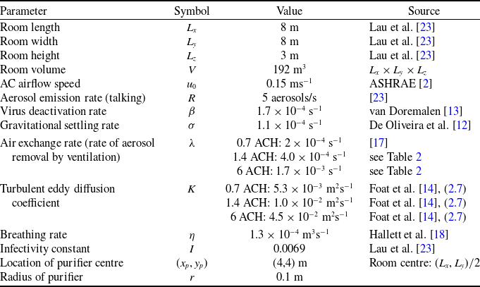
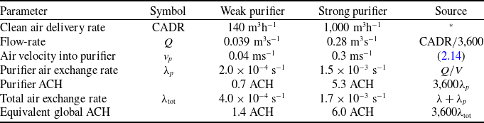
 λ=2×10⁻⁴
 −1
−1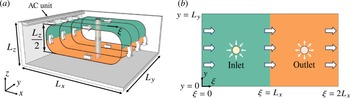
 Lx
Lx Ly
Ly Lz
Lz ξ
ξ (ξ,y)
(ξ,y)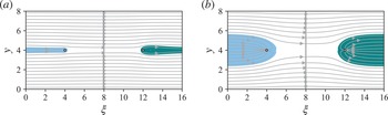
 (ξ,y)
(ξ,y) vp=0.04
 vp=0.3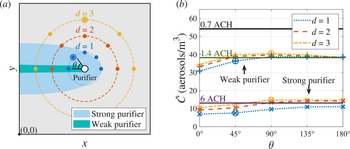
 x0
x0 C¯
C¯ +
+ ×
× x0
x0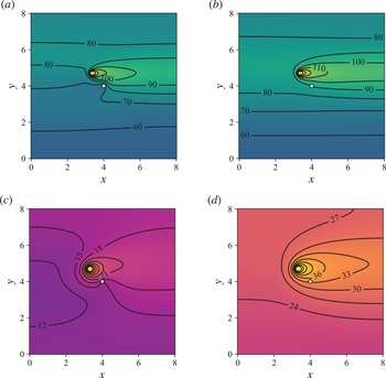
 C
C x0
x0 (d,θ)=(1,45∘)
 Cp
Cp Cg
Cg 3
3 Cp
Cp Cg
Cg 3
3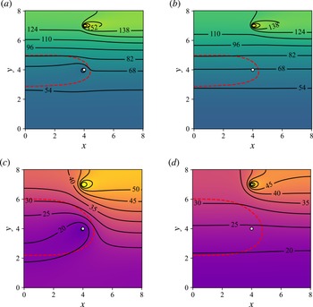
 C
C x0
x0 (d,θ)=(3,90∘)
 Cp
Cp Cg
Cg 3
3 Cp
Cp Cg
Cg 3
3 Cp=Cg
Cp=Cg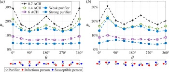
 P
P xs
xs ϕ=180∘
 ϕ=90∘
ϕ=90∘ θ
θ
 Open access

