





1. Introduction
Sea level rise projections rely on accurate predictions of ice mass loss from Antarctica (Ligtenberg and others, Reference Ligtenberg, van de Berg, van den Broeke, Rae and van Meijgaard2013; Dutton and others, Reference Dutton2015; DeConto and Pollard, Reference DeConto and Pollard2016; Pattyn and Morlighem, Reference Pattyn and Morlighem2020). Basal ice temperature is a key factor influencing basal sliding, basal melt, subglacial hydrology and the ice-flow regime (Engelhardt, Reference Engelhardt2004; Pattyn, Reference Pattyn2010; Kyrke-Smith and others, Reference Kyrke-Smith, Katz and Fowler2014; Seroussi and others, Reference Seroussi, Ivins, Wiens and Bondzio2017; Dawson and others, Reference Dawson, Schroeder, Chu, Mantelli and Seroussi2022), and hence mass loss (Dawson and others, Reference Dawson, Schroeder, Chu, Mantelli and Seroussi2022). If basal temperatures reach the pressure-melting point, basal sliding and basal melt may occur, allowing for much faster flow than that driven solely by internal ice deformation. These faster-flowing regions contribute disproportionately to ice discharge and dynamic mass loss and are often more responsive to external forcing. Basal thermal conditions also influence subglacial hydrology because basal temperatures at or close to the pressure-melting point favor the presence of liquid water, thereby controlling effective pressure and basal resistance. Importantly, the relevance of basal temperature extends beyond simply determining whether the bed has already reached the pressure-melting point. Even when basal ice remains below the pressure-melting point, warmer basal conditions imply softer ice and thus lower effective viscosity, as ice stiffness decreases by nearly three orders of magnitude between −20°C and 0°C (Paterson, Reference Paterson1994). Moreover, spatial variations in basal temperature below the melting point help distinguish cold-based, near-temperate and transitional basal regimes, and thereby identify regions that may be particularly sensitive to relatively small perturbations in geothermal heat flux (GHF) or frictional heating that could shift basal conditions toward thaw (Dawson and others, Reference Dawson, Schroeder, Chu, Mantelli and Seroussi2022). Capturing precise basal temperatures is a critical prerequisite for correctly spinning up and constraining vertical temperature profiles when solving coupled thermomechanical equations (Park and others, Reference Park, Jin, Morlighem and Lee2024). Finally, basal thermal conditions are important for paleoclimate applications, since the selection of suitable drilling sites for ‘Oldest Ice’ cores requires avoiding areas with significant basal melting that would remove the oldest ice near the bed (Fischer and others, Reference Fischer2013).
Despite its importance, the continental-scale distribution of basal thermal state remains poorly constrained. Our knowledge relies on three main sources: direct borehole measurements, which are accurate but sparse; geophysical inferences from radar and seismic data, which have broader but still incomplete coverage; and simulation results from ice-sheet models (MacGregor and others, Reference MacGregor2016, Reference MacGregor2022; Matsuoka and others, Reference Matsuoka, MacGregor and Pattyn2012). Thermodynamic ice-sheet models are widely used to simulate thermal states (Budd and others, Reference Budd, Jenssen and Coutts1994; Pattyn, Reference Pattyn2010; Seroussi and others, Reference Seroussi2019). However, significant uncertainties persist, primarily due to poorly constrained GHF (Reading and others, Reference Reading2022). While three-dimensional (3-D) full-Stokes models provide physically comprehensive descriptions of ice flow, their substantial computational cost restricts large-scale ensemble simulations needed for systematic exploration of basal temperature sensitivity to boundary condition uncertainties, particularly GHF. Machine learning (ML) encompasses a broad set of approaches that are increasingly being applied across Earth system science, including oceanography (Ducournau and Fablet, Reference Ducournau and Fablet2016; Lou and others, Reference Lou, Lv, Dang, Su and Li2023), climatology (Rhee and Im, Reference Rhee and Im2017; Jiang and others, Reference Jiang, Xu and Wei2018) and hydrology (Marçais and De Dreuzy, Reference Marçais and De Dreuzy2017; Xu and Liang, Reference Xu and Liang2021). In cryosphere research, recent studies have used ML for tasks such as automated glacier mapping (Lu and others, Reference Lu, Zhang, Shangguan and Yang2021; Xie and others, Reference Xie, Asari and Haritashya2021), ice thickness estimation (Werder and others, Reference Werder, Huss, Paul, Dehecq and Farinotti2020; Jouvet and others, Reference Jouvet, Cordonnier, Kim, Lüthi, Vieli and Aschwanden2022), calving front extraction (Zhang and others, Reference Zhang, Liu and Huang2019; Mohajerani and others, Reference Mohajerani, Jeong, Scheuchl, Velicogna, Rignot and Milillo2021) and surface mass balance estimation (Anilkumar and others, Reference Anilkumar, Bharti, Chutia and Aggarwal2023; van der Meer and others, Reference van der Meer, Zekollari, Huss, Bolibar, Sjursen and Farinotti2025). While several studies have employed ML in related applications, such as inferring basal friction coefficients and reconstructing glacier-wide surface mass balance (Bolibar and others, Reference Bolibar, Rabatel, Gouttevin, Galiez, Condom and Sauquet2020; Umlauft and others, Reference Umlauft2023), the use of ML as direct emulators for basal thermal properties remains largely underexplored.
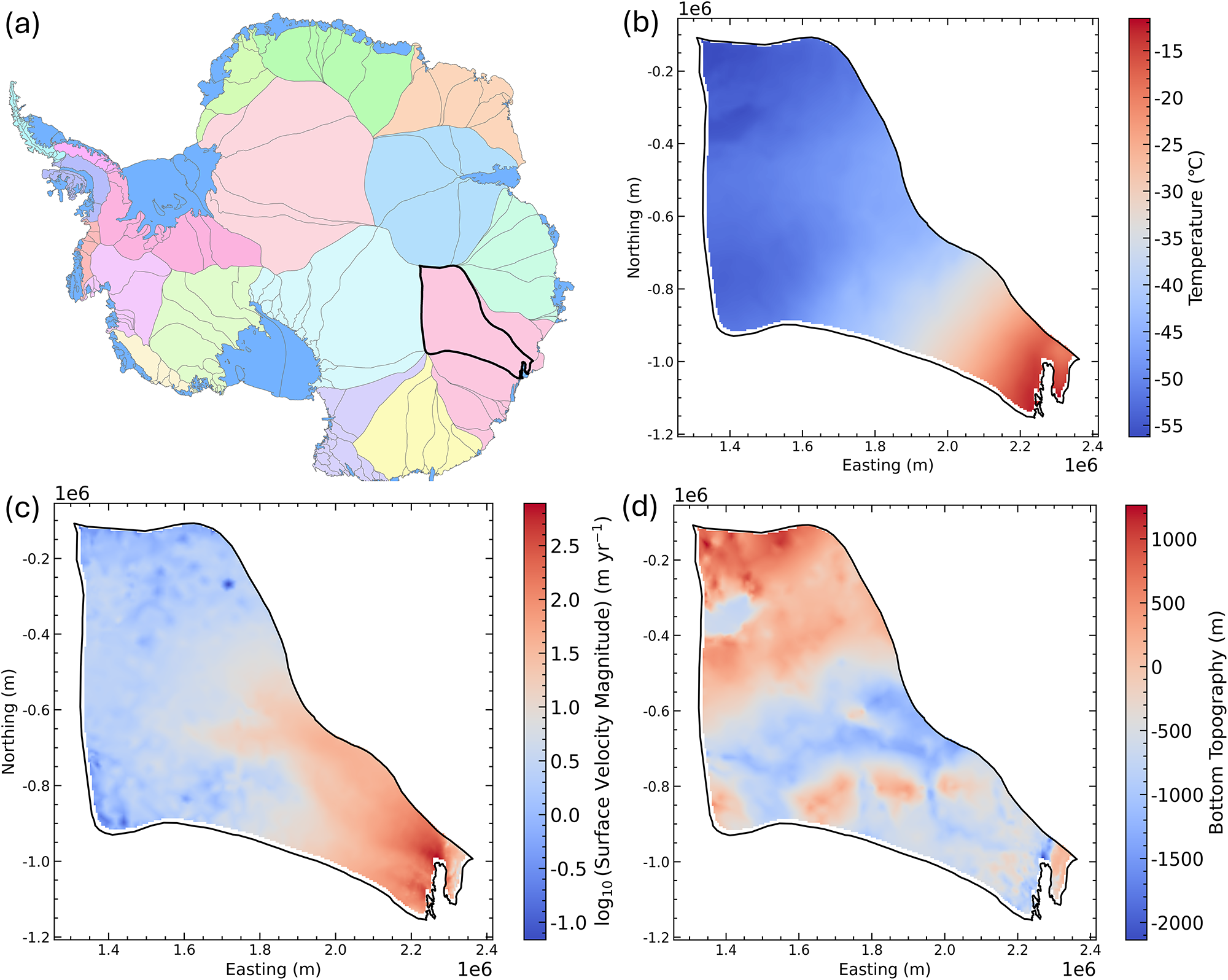
Totten Glacier (Fig. 1) is one of the most vulnerable glaciers in East Antarctica to a warming climate (Li and others, Reference Li, Rignot, Mouginot and Scheuchl2016; Dow and others, Reference Dow, McCormack, Young, Greenbaum, Roberts and Blankenship2020). It has the largest ice discharge in East Antarctica (Rignot, Reference Rignot2006), and the drainage basin of Totten Glacier contains enough ice to raise global sea level by approximately 3.9 m. The glacier has also experienced significant thinning and mass loss during recent decades (Li and others, Reference Li, Rignot, Morlighem, Mouginot and Scheuchl2015). Recent studies indicate that Totten Glacier is losing mass at a rate of approximately 7 Gt yr−1, with 73% of this loss attributed to ice-sheet dynamics (Li and others, Reference Li, Rignot, Mouginot and Scheuchl2016). As the primary outlet glacier of the Aurora Subglacial Basin, a marine basin below sea level, it is of particular concern because its reverse-sloping bed geometry may make it susceptible to marine ice-sheet instability (Schoof, Reference Schoof2007; Sergienko and others, Reference Sergienko, Haseloff, Robel and Wingham2026). Beyond this large-scale geometric control, the stability of Totten Glacier and ice flow dynamics are sensitive to subglacial hydrology and basal temperature. GHF, the heat flow from Earth’s crust to the ice-bed interface, critically influences the ice temperature profile and consequently affects ice rheology and flow dynamics (Burton-Johnson and others, Reference Burton-Johnson, Dziadek and Martin2020; Dziadek and others, Reference Dziadek, Ferraccioli and Gohl2021). However, there are currently multiple GHF maps available for Antarctica, based on various datasets and methods, including seismic models (Shapiro and Ritzwoller, Reference Shapiro and Ritzwoller2004; An and others, Reference An2015; Shen and others, Reference Shen, Wiens, Lloyd and Nyblade2020), rock magnetic models (Purucker, Reference Purucker2012; Martos and others, Reference Martos, Catalán, Jordan, Golynsky, Golynsky, Eagles and Vaughan2017) and multivariate or ML approaches (Dziadek and others, Reference Dziadek, Gohl, Diehl and Kaul2017; Lösing and Ebbing, Reference Lösing and Ebbing2021; Stål and others, Reference Stål, Reading, Halpin and Whittaker2021; Haeger and others, Reference Haeger, Petrunin and Kaban2022). The various spatial GHF datasets result in significantly different distributions of basal ice temperatures that then impact ice-sheet model simulations (Kang and others, Reference Kang, Zhao, Wolovick and Moore2022; Huang and others, Reference Huang, Zhao, Wolovick, Ma and Moore2024). The substantial computational cost of high-resolution full-Stokes ice-sheet models limits comprehensive basal temperature simulations across all GHF datasets, highlighting the demand for efficient predictive emulators of basal ice temperature.
(a) Location of Totten Glacier in Antarctica; (b) surface ice temperature; (c) surface velocity magnitude; (d) bed elevation. The solid black line outlines the study domain, which excludes the Totten Ice Shelf.

Figure 1 Long description
A) A map of East Antarctica showing various regions with labeled basins, each in different colors. B) A thematic map of surface ice temperature in the Totten Glacier area, ranging from -55 to -15 degrees Celsius. The temperature increases from the inland areas toward the eastern edge. C) A map displaying the log10 surface velocity magnitude, with values from 0 to 2.5 meters per year. Higher velocities are observed near the eastern boundary. D) A map of bed elevation, ranging from -2000 to 1000 meters, with lower elevations inland and higher elevations toward the eastern edge. Each map includes a solid black line outlining the study domain, excluding the Totten Ice Shelf. The maps are oriented with northing increasing upward and easting increasing to the right. The color scales represent different variables: blue indicates lower values and red indicates higher values. The maps provide insights into the temperature, velocity and elevation patterns within the outlined domain.
In this study, we develop and evaluate an ML framework to serve as a computationally efficient emulator for a full-Stokes ice-sheet model, with the specific goal of predicting basal ice temperature for Totten Glacier. We train and compare three distinct nonlinear models—random forest (RF), XGBoost and neural network (NN)—against a traditional linear regression baseline to highlight the system’s nonlinear dynamics. The emulators use bedrock elevation, ice thickness, surface temperature, observed surface velocity and GHF as inputs, and predict basal ice temperature; in additional experiments involving simultaneous prediction, basal melt rate is also included as an output. A detailed description of the ML models is provided in Section 2.2. Our analysis is multifaceted: we not only assess the models’ predictive accuracy but also determine the minimum number of numerical simulations required for robust training, test the models’ capacity for simultaneous prediction of both basal ice temperature and melt rate, and use state-of-the-art interpretability techniques to identify the dominant physical drivers of these subglacial conditions. Once trained on ice-sheet model outputs, this emulator enables rapid predictions of basal thermal conditions, thereby providing a computationally efficient alternative to extensive continental-scale ice dynamics simulations required for sensitivity analysis and uncertainty quantification.
2. Data and methods
2.1. Preparation of features and training dataset
In this study, the ML emulators are trained using inputs and outputs from Huang and others (Reference Huang, Zhao, Wolovick, Ma and Moore2024), in which a coupled modeling workflow was used to generate final steady-state basal thermal fields for Totten Glacier under eight GHF scenarios. The emulator targets extracted from the steady-state simulations are basal ice temperature and basal melt rate. The input data of the ice-sheet model include surface and bottom elevation, ice thickness, surface temperature, surface velocity and GHF. Given that the surface topography of grounded ice can be reconstructed by bottom topography plus ice thickness and is strongly correlated with surface ice temperature (Pearson r = −0.98), we excluded surface topography from the input feature set. The final set of five variables represents the key quantities that govern heat and momentum conservation in the physical ice-sheet model and also serves as the input variables for the ML emulators. Bedrock elevation and ice thickness data are sourced from the MEaSUREs BedMachine Antarctica, Version 2 (Morlighem and others, Reference Morlighem2020), consistent with the numerical workflow of Huang and others (Reference Huang, Zhao, Wolovick, Ma and Moore2024), from which the emulator training data were derived. Surface temperature data are obtained from ALBMAP v1 with a resolution of 5 km (Le Brocq and others, Reference Le Brocq, Payne and Vieli2010). The observed surface ice velocity data are from the MEaSUREs InSAR-Based Antarctica Ice Velocity Map, version 2, with a resolution of 450 m (Rignot and others, Reference Rignot, Mouginot and Scheuchl2017). The GHF fields are from eight sources: Purucker (Reference Purucker2012), Shapiro and Ritzwoller (Reference Shapiro and Ritzwoller2004), An and others (Reference An2015), Shen and others (Reference Shen, Wiens, Lloyd and Nyblade2020), Stål and others (Reference Stål, Reading, Halpin and Whittaker2021), Haeger and others (Reference Haeger, Petrunin and Kaban2022), Lösing and Ebbing (Reference Lösing and Ebbing2021) and Martos and others (Reference Martos, Catalán, Jordan, Golynsky, Golynsky, Eagles and Vaughan2017). As GHF does not directly influence sub-ice-shelf basal temperature, the ice shelf is excluded from this study.
In Huang and others (Reference Huang, Zhao, Wolovick, Ma and Moore2024), the basal thermal state of Totten Glacier was estimated using an off-line coupling between a forward model and an inverse model. The forward model consists of an improved shallow-ice-approximation thermomechanical model with a subglacial hydrology model (Wolovick and others, Reference Wolovick, Moore and Zhao2021), and aims to provide an appropriate vertical temperature profile for the inverse model. The full-Stokes inverse model is used to adjust the spatial distribution of the basal friction coefficient to minimize the misfit between simulated and observed surface velocities. The modeled velocity is obtained by solving a 3-D full-Stokes model subject to a basal sliding condition. Ice viscosity in the full-Stokes model is strongly dependent on ice temperature. Huang and others (Reference Huang, Zhao, Wolovick, Ma and Moore2024) employed a finite-element mesh in their ice model, with mesh sizes ranging from a maximum of 20 km far inland to a minimum of 800 m in regions with fast ice flow. We take the result at every node of the 2-D horizontal footprint mesh as the data used for ML model training and evaluation. We did not perform any regular-grid interpolation of the ice-sheet model outputs because interpolating the data onto a regular grid could introduce errors that are not inherent to the ice-sheet model results. There are 11 620 nodes in the 2-D mesh. In other words, for each GHF dataset, 11 620 samples are used for ML emulator.
Huang and others (Reference Huang, Zhao, Wolovick, Ma and Moore2024) generated steady-state basal thermal outputs for eight GHF scenarios. In the present study, six of these scenarios were used to form the development dataset for model training and internal validation, whereas the Purucker (Reference Purucker2012) and Martos and others (Reference Martos, Catalán, Jordan, Golynsky, Golynsky, Eagles and Vaughan2017) scenarios were withheld entirely and used only as an independent test set. We selected these two scenarios because they produce the lowest and highest mean basal ice temperatures, respectively, and therefore provide a deliberately challenging test of generalization across unseen GHF forcings. We note, however, that this should be interpreted as testing generalization across withheld GHF scenarios within the Totten Glacier setting, rather than as a true test of transferability to a different glacier system. Separately, to understand how the amount of training data impacts prediction accuracy, we systematically vary the number of simulations used for training from one to seven. For each training set size, we tested all possible combinations of simulation datasets, training the model on the selected simulations and evaluating it on the remaining GHF simulations that were not included in training. This process allows us to determine the minimum number of expensive ice-sheet simulations required to train an effective ML emulator.
2.2. ML emulation
In this study, we use ML to create a computationally efficient surrogate model (or ‘emulator’) that learns the relationship between inputs and outputs from a complex physical ice-sheet model. Unlike traditional simulations that solve explicit physical equations, a data-driven approach learns these relationships directly from simulation results (Liu and others, Reference Liu, Koo and Rahnemoonfar2024). We employ a supervised learning framework, where an algorithm is trained on a dataset containing both the model inputs (e.g. GHF, basal topography) and outputs (the basal ice temperature calculated by the ice-sheet model). The primary goal is to determine how effectively an ML emulator can reproduce the basal thermal state simulated by the numerical ice-sheet model, but at a fraction of the computational cost. This emulator should be viewed as a diagnostic tool for estimating the present-day thermal state under different GHF fields, rather than as a prognostic module that can be directly embedded in evolving transient simulations to evaluate how the thermal state evolves, since it has been trained on steady-state velocities and temperatures. To enhance the interpretability of the ML models, we incorporated Shapley Additive Explanations (SHAP) values to explain model predictions and connect the data-driven findings back to glaciological processes. To compare model performance, we also used a baseline model: multiple linear regression.
We select three ML emulators that learn in different ways. RF is an ensemble method, meaning it combines multiple base models to improve predictive capability. The base model it uses is a binary decision tree (Supplementary Fig. S1), represented as a tree structure. By adjusting different parameter settings, RF model builds hundreds or thousands of different decision trees—an entire ‘forest’ (Supplementary Fig. S1). Each tree is trained by a random subset of the training data. To make a final prediction, the model asks every tree in the forest for its predicted value and calculates the average. This process, known as ‘bagging’, makes the final prediction more robust and significantly mitigates the risk of overfitting, although it does not make the model entirely immune to it (Breiman, Reference Breiman2001). The strength of RF is its ability to automatically capture complex, nonlinear interactions (e.g. the effect of GHF may differ in thick vs thin ice) without requiring pre-defined physical equations.
Like RF, XGBoost is also an ensemble of decision trees, but it builds them in a sequential way known as ‘boosting’ (Chen and Guestrin, Reference Chen and Guestrin2016). XGBoost builds trees in a sequential manner, where each new tree is added to correct the errors of earlier ones, using techniques such as greedy algorithms for split point selection, which improve both model performance and computational speed. The final prediction is a weighted sum of the predictions from all the trees (Supplementary Fig. S2). This sequential, error-correcting process makes XGBoost often outperform other methods.
The NN model is inspired by the structure of the brain and is fundamentally different from tree-based models. It processes information through interconnected layers of computational ‘neurons’ or nodes (Dongare and others, Reference Dongare, Kharde and Kachare2012) (Supplementary Fig. S3). The input data (GHF, bottom topography, etc.) are fed into the first layer. NN models use a weighted combination of input features along with nonlinear functions (called activation functions) such as sigmoid and tanh to produce the activations of the neurons in the next layer (called a hidden layer) (Supplementary Fig. S3a). Multiple hidden layers form an NN and ultimately give the predicted output, which is basal ice temperature in our case (Supplementary Fig. S3b). NNs have been shown to approximate any continuous function even with a single hidden layer and sufficient neurons (Hornik, Reference Hornik1991). NNs can fit complex functional relationships through multilayer structures and nonlinear activation functions, and are suitable for various complex tasks.
2.3. Hyperparameter fine-tuning and performance evaluation
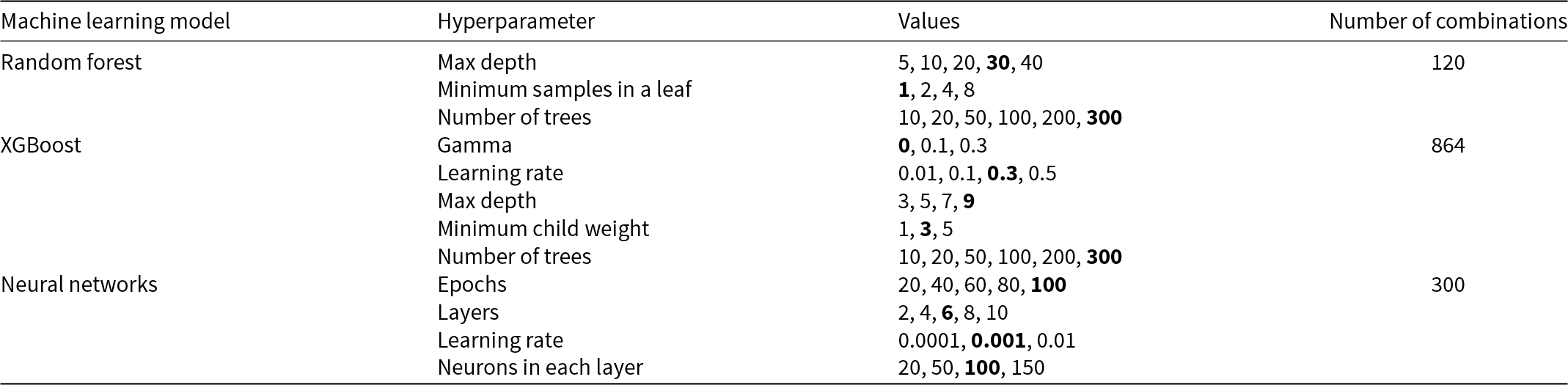
ML emulators are inherently data-driven, and their performance is influenced not only by the internal parameters obtained automatically during training but also by hyperparameters, which are manually set before training. These hyperparameters can be regarded as analogous to prescribed constant parameters in ice-sheet models, such as the number of trees in an RF or the number of neurons within an NN model. We use a process called k-fold cross-validation on our development dataset of six simulations (all except those from Purucker (Reference Purucker2012) and Martos and others (Reference Martos, Catalán, Jordan, Golynsky, Golynsky, Eagles and Vaughan2017)). The dataset is randomly split into three equal parts, or ‘folds’. The emulator is trained on two folds, and its performance is evaluated on the third (the validation fold). This process was repeated three times, ensuring each fold was used for validation exactly once. It is noted that the development dataset was randomly split and used only for hyperparameter selection, while the main reported model errors come from the independent withheld-GHF test set. We tested numerous combinations of hyperparameters listed in Table 1 and selected the one that yielded the best average performance across the three validation folds. Finally, the final emulators were retrained on the entire development dataset using these optimal settings. The NN model is a fully connected feed-forward model implemented in Keras, with ReLU activation in the hidden layers, Glorot uniform weight initialization and the Adam optimizer. The number of hidden layers, neurons per layer, learning rate and number of training epochs were optimized by grid search, while the batch size was fixed at 128. No additional dropout or L2 weight decay was used in the final implementation. Z-score normalization (standardization) was applied to the input features for all three ML models.
Hyperparameter combinations for each model.

Table 1 Long description
The table lists hyperparameter search ranges and the total number of parameter combinations evaluated for three machine learning models. Random Forest varies max depth from 5 to 40, minimum samples in a leaf from 1 to 8, and number of trees from 10 to 300, for 120 combinations. XGBoost varies gamma from 0 to 0.3, learning rate from 0.01 to 0.5, max depth from 3 to 9, minimum child weight from 1 to 5, and number of trees from 10 to 300, for 864 combinations. Neural Networks vary epochs from 20 to 100, layers from 2 to 10, learning rate from 0.0001 to 0.01, and neurons per layer from 20 to 150, for 300 combinations. Across models, the number of trees is explored over the same six values for Random Forest and XGBoost, while learning rate is tuned for XGBoost and Neural Networks but on different scales. The totals reflect the size of each grid search and do not indicate which settings performed best.
Note: The bold numbers in the table represent the optimal hyperparameter combination for each model.
To evaluate emulator performance, we calculated three statistical metrics on the test dataset: the coefficient of determination (R 2), root mean square error (RMSE) and mean absolute error (MAE). The coefficient of determination (R 2) quantifies the proportion of variance in the target data that is explained by the model. A perfect fit yields R 2 = 1, whereas R 2 = 0 indicates no improvement over simply predicting the mean of the target values. R 2 can also be negative when the model performs worse than this mean-based reference. RMSE represents the absolute deviations between the target and predicted values. RMSE is sensitive to large errors, particularly when outliers or large deviations exist, and penalizes large discrepancies. MAE is the average of the absolute prediction errors, providing a straightforward and intuitive measure of prediction accuracy.
2.4. Interpreting model predictions using SHAP
While our ML models demonstrate high predictive accuracy, their complex internal structures can make it difficult to understand precisely how they arrive at a prediction. To overcome this ‘black-box’ problem and extract meaningful scientific insights, we employed SHAP, a method for interpreting the output of any ML model (Lundberg and Lee, Reference Lundberg and Lee2017). The core idea behind SHAP is to explain an individual prediction by quantifying exactly how much each input variable contributed to pushing the prediction away from a baseline value (e.g. the average predicted basal ice temperature across the entire dataset). For every sample prediction the model makes, each input variable is assigned a SHAP value, which has two key properties:
(1) Direction: The sign of the value shows the direction of the effect. A positive SHAP value means that a variable (e.g. a high GHF value) pushed the prediction toward a warmer temperature, which is defined as a positive contribution. A negative SHAP value means it pushed the prediction toward a lower temperature, referred to as a negative contribution.
(2) Magnitude: The size of the value reveals the importance of that variable’s contribution to that specific prediction.
A major strength of SHAP is that these contributions are additive; the sum of all the SHAP values for a single sample prediction perfectly explains the difference between that prediction and the baseline average. This allows us to analyze model behavior on a case-by-case basis, for instance by assessing whether a region of warm basal ice was primarily associated with high GHF, greater ice thickness or other local boundary conditions, as inferred from the emulator. To assess which variables are most important overall, we can aggregate these individual explanations. We rank the input variables by their mean absolute SHAP value across all points in our test dataset. This metric quantifies the average impact each variable has on the model’s predictions, providing a robust and consistent measure of global feature importance. By using SHAP, we can transform our ML emulators from simple prediction tools into instruments for investigating the complex physical relationships governing the basal thermal state of Totten Glacier.
3. Results
3.1. Performance of ML emulators
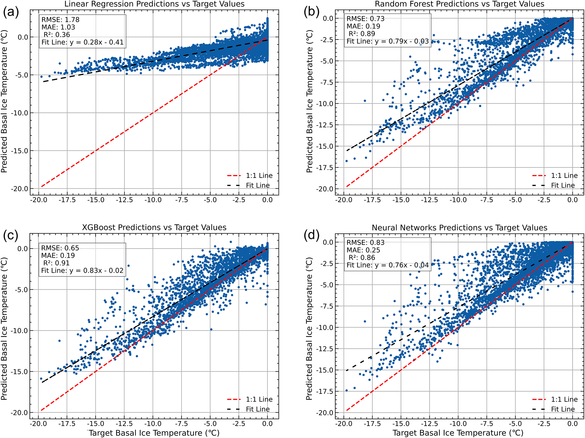
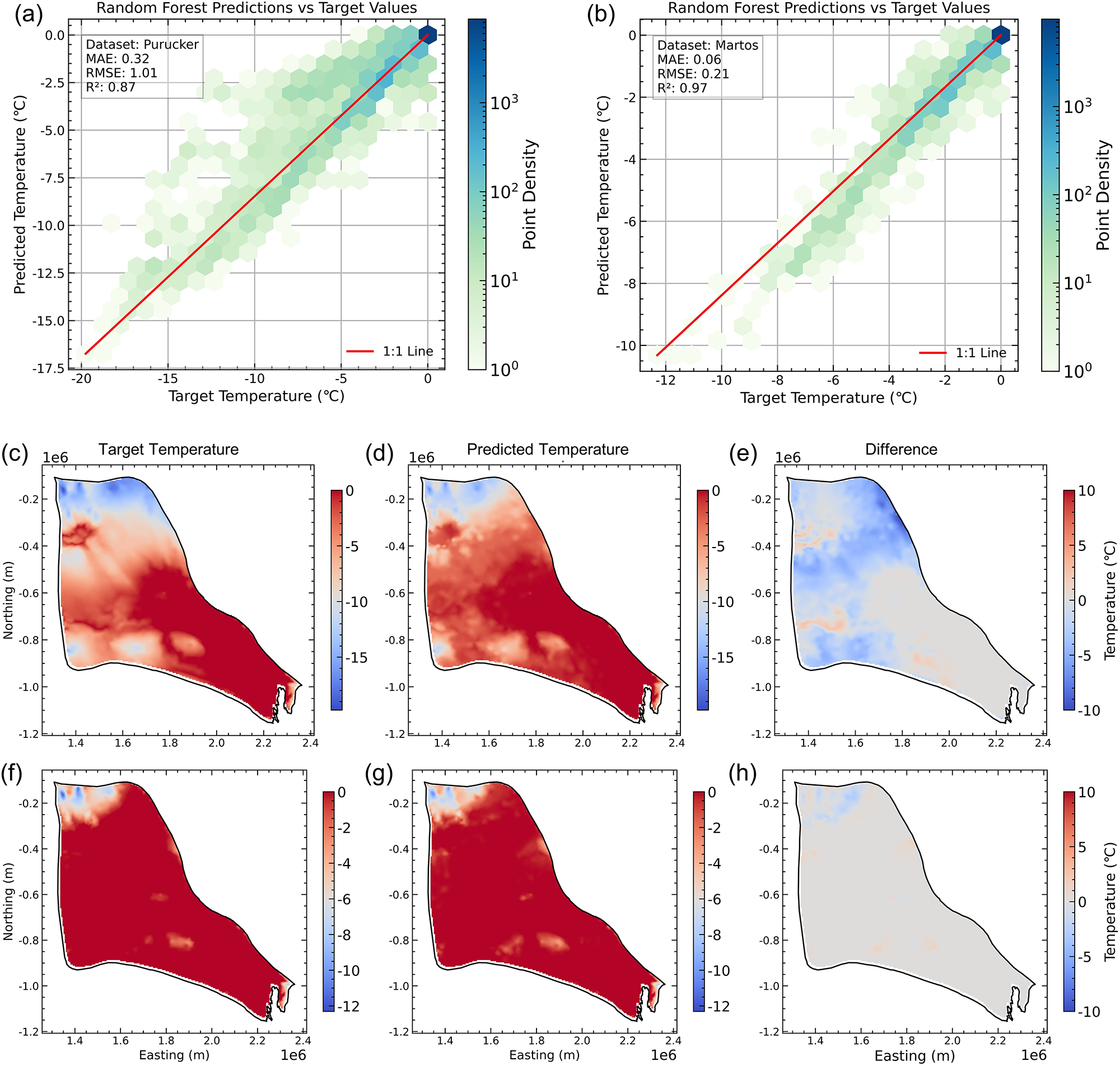
The RF emulator exhibits superior predictive performance on the combined test dataset (Purucker, Reference Purucker2012; Martos and others, Reference Martos, Catalán, Jordan, Golynsky, Golynsky, Eagles and Vaughan2017), achieving an RMSE of 0.73°C, a coefficient of determination (R 2) value of 0.89 and an MAE of 0.19°C (Fig. 2b). To assess the emulator’s robustness, we evaluated its performance on the two test simulations individually. On the Purucker (Reference Purucker2012) data, the RF emulator replicates the main spatial patterns of basal temperature (R 2 = 0.87), though it exhibits a tendency to slightly overestimate temperatures in colder regions, particularly in slow-flowing interior areas with elevated basal topography (Fig. 3e). In contrast, the RF emulator performs particularly well on the Martos and others (Reference Martos, Catalán, Jordan, Golynsky, Golynsky, Eagles and Vaughan2017) dataset, achieving close agreement between predictions and simulation-derived data: R 2 approximately 0.97, RMSE of 0.21°C and MAE < 0.1°C (Fig. 3b). Spatial predictions closely matched the target basal ice temperatures across most of the glacier, with only minor underestimation at the southwest corner of the glacier (Fig. 3h).
Scatter plot depicting prediction performance of each emulator on the two test datasets (N = 23 240), Purucker (Reference Purucker2012) dataset and Martos and others (Reference Martos, Catalán, Jordan, Golynsky, Golynsky, Eagles and Vaughan2017) dataset: (a) linear regression (LR); (b) random forest (RF); (c) extreme gradient boosting (XGBoost); (d) neural networks (NN). Each data point represents the result at a node of the 2-D horizontal footprint mesh used in Huang and others (Reference Huang, Zhao, Wolovick, Ma and Moore2024).

Figure 2 Long description
The image A showing a scatter plot titled Linear Regression Predictions vs Target Values. The x-axis label is Target Basal Ice Temperature (degree celsius). The y-axis label is Predicted Basal Ice Temperature (degree celsius). The x-axis range is negative 20.0 to 0.0. The y-axis range is negative 20.0 to 0.0. Text box values: RMSE: 1.78, MAE: 0.36, R2: 0.13. A line label reads Fit Line: y equals 0.28x minus 0.41. A legend lists 1:1 Line and Fit Line. The image B showing a scatter plot titled Random Forest Predictions vs Target Values. The x-axis label is Target Basal Ice Temperature (degree celsius). The y-axis label is Predicted Basal Ice Temperature (degree celsius). The x-axis range is negative 20.0 to 0.0. The y-axis range is negative 20.0 to 0.0. Text box values: RMSE: 0.73, MAE: 0.19, R2: 0.89. A line label reads Fit Line: y equals 0.79x minus 0.39. A legend lists 1:1 Line and Fit Line. The image C showing a scatter plot titled XGBoost Predictions vs Target Values. The x-axis label is Target Basal Ice Temperature (degree celsius). The y-axis label is Predicted Basal Ice Temperature (degree celsius). The x-axis range is negative 20.0 to 0.0. The y-axis range is negative 20.0 to 0.0. Text box values: RMSE: 0.69, MAE: 0.20, R2: 0.90. A line label reads Fit Line: y equals 0.83x minus 0.02. A legend lists 1:1 Line and Fit Line. The image D showing a scatter plot titled Neural Networks Predictions vs Target Values. The x-axis label is Target Basal Ice Temperature (degree celsius). The y-axis label is Predicted Basal Ice Temperature (degree celsius). The x-axis range is negative 20.0 to 0.0. The y-axis range is negative 20.0 to 0.0. Text box values: RMSE: 0.83, MAE: 0.25, R2: 0.86. A line label reads Fit Line: y equals 0.78x minus 0.17. A legend lists 1:1 Line and Fit Line.
Prediction performance (scatter point density), target basal ice temperature, predicted basal ice temperature and their difference (target minus predicted) for RF emulator on Purucker (Reference Purucker2012) dataset (a, c–e) and Martos and others (Reference Martos, Catalán, Jordan, Golynsky, Golynsky, Eagles and Vaughan2017) dataset (b, f–h).

Figure 3 Long description
The image A showing a scatter plot titled Random Forest Predictions vs Target Values. Text: Dataset: Purucker. MAE: 0.32. RMSE: 0.73. R2: 0.87. The horizontal axis label is Target Temperature (degree celsius) with values from minus 20 to 0. The vertical axis label is Predicted Temperature (degree celsius) with values from minus 17.5 to 0. A diagonal line is labeled 1:1 Line. A vertical axis on the right is labeled Point Density with values 10 superscript 0, 10 superscript 1, 10 superscript 2, 10 superscript 3. The plotted points form a diagonal band that follows the 1:1 Line, with the highest point density along the diagonal. The image B showing a scatter plot titled Random Forest Predictions vs Target Values. Text: Dataset: Martos. MAE: 0.06. RMSE: 0.21. R2: 0.97. The horizontal axis label is Target Temperature (degree celsius) with values from minus 12 to 0. The vertical axis label is Predicted Temperature (degree celsius) with values from minus 10 to 0. A diagonal line is labeled 1:1 Line. A vertical axis on the right is labeled Point Density with values 10 superscript 0, 10 superscript 1, 10 superscript 2, 10 superscript 3. The plotted points form a narrow diagonal band close to the 1:1 Line, with the highest point density along the diagonal. The image C showing a map titled Target Temperature. The horizontal axis label is Easting (m) with values 0, 0.5e6, 1.0e6, 1.5e6, 2.0e6, 2.5e6. The vertical axis label is Northing (m) with values minus 1.0e6, minus 0.5e6, 0, 0.5e6. A vertical scale bar is labeled Temperature (degree celsius) with values minus 15, minus 10, minus 5, 0, 5. The mapped region contains broad areas near the upper end of the scale and smaller areas near the lower end of the scale. The image D showing a map titled Predicted Temperature. The horizontal axis label is Easting (m) with values 0, 0.5e6, 1.0e6, 1.5e6, 2.0e6, 2.5e6. The vertical axis label is Northing (m) with values minus 1.0e6, minus 0.5e6, 0, 0.5e6. A vertical scale bar is labeled Temperature (degree celsius) with values minus 15, minus 10, minus 5, 0, 5. The mapped region shows a spatial pattern similar to the Target Temperature map, with broad areas near the upper end of the scale and smaller areas near the lower end of the scale. The image E showing a map titled Difference. The horizontal axis label is Easting (m) with values 0, 0.5e6, 1.0e6, 1.5e6, 2.0e6, 2.5e6. The vertical axis label is Northing (m) with values minus 1.0e6, minus 0.5e6, 0, 0.5e6. A vertical scale bar is labeled Temperature (degree celsius) with values minus 10, minus 5, 0, 5, 10. The mapped region contains large areas near the 0 value on the scale and smaller patches toward the negative and positive ends of the scale. The image F showing a map. The horizontal axis label is Easting (m) with values 0, 0.5e6, 1.0e6, 1.5e6, 2.0e6, 2.5e6. The vertical axis label is Northing (m) with values minus 1.0e6, minus 0.5e6, 0, 0.5e6. A vertical scale bar is labeled Temperature (degree celsius) with values minus 12, minus 10, minus 8, minus 6, minus 4, minus 2. The mapped region shows most areas near the upper end of this scale, with smaller areas toward the lower end. The image G showing a map. The horizontal axis label is Easting (m) with values 0, 0.5e6, 1.0e6, 1.5e6, 2.0e6, 2.5e6. The vertical axis label is Northing (m) with values minus 1.0e6, minus 0.5e6, 0, 0.5e6. A vertical scale bar is labeled Temperature (degree celsius) with values minus 12, minus 10, minus 8, minus 6, minus 4, minus 2. The mapped region shows most areas near the upper end of this scale, with smaller areas toward the lower end. The image H showing a map. The horizontal axis label is Easting (m) with values 0, 0.5e6, 1.0e6, 1.5e6, 2.0e6, 2.5e6. The vertical axis label is Northing (m) with values minus 1.0e6, minus 0.5e6, 0, 0.5e6. A vertical scale bar is labeled Temperature (degree celsius) with values minus 10, minus 5, 0, 5, 10. The mapped region contains large areas near the 0 value on the scale and smaller patches toward the negative and positive ends of the scale. Across the eight sub-images, the two scatter plots compare Predicted Temperature (degree celsius) against Target Temperature (degree celsius) using a 1:1 Line and the six maps show Target Temperature, Predicted Temperature and Difference using Temperature (degree celsius) scale bars.
The XGBoost emulator, another tree-based ML approach, yields a comparable and even marginally superior performance to the RF emulator (Fig. 2c). The emulator achieves an R 2 value of 0.91, and an RMSE of 0.65°C on the test dataset, with its regression line closely aligning with the 1:1 reference line, indicating strong agreement between predicted and target values. Spatially, the XGBoost emulator produces error patterns qualitatively similar to those of the RF emulator (Supplementary Fig. S4).
The NN emulator, while performing adequately overall, demonstrates lower predictive capability compared to the tree-based emulators (Fig. 2d). With an R 2 value of 0.86, the NN emulator’s accuracy is somewhat reduced relative to both RF and XGBoost. The NN captures the large-scale distribution of basal temperature but struggles to resolve finer-scale, local variations with the same precision (Supplementary Fig. S5).
In summary, the three ML emulators (RF, XGBoost and NN) significantly outperform the linear baseline emulator in predictive performance (Fig. 2a). This result indicates that the relationships between the glaciological input variables and the resulting basal temperature are inherently complex and nonlinear, requiring the flexibility of ML approaches to be emulated accurately.
3.2. The influence of training dataset size
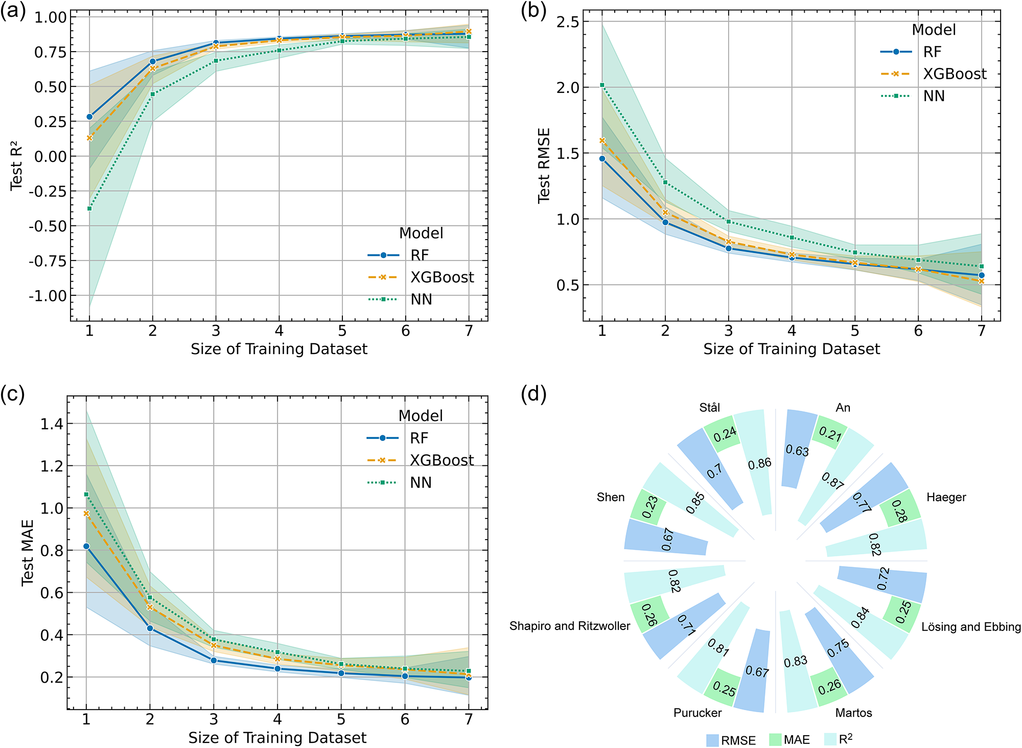
While our final emulators are trained on six GHF simulations, the size of the training dataset is a critical factor that can impact predictive performance. To investigate this, we systematically evaluate how emulator accuracy changes as the number of simulations in the training set is varied from one to seven. For each training-set size, the emulator is trained on the selected subset of GHF simulations and evaluated on the remaining GHF simulations that were not used for training. As illustrated by the learning curves in Fig. 4, all three ML emulators show a clear trend: performance improves as the number of training simulations increases. The R 2 value rises steeply at first, before beginning to plateau once the training set size reaches five simulations. This trend indicates that with five or six simulations, the emulators have been exposed to enough variability to learn the underlying physical relationships effectively. However, even with consistent training set sizes, emulator performance exhibits variability across different dataset combinations. Beyond six training simulations, the intervals of the R 2 plot broaden, indicating performance degradation for certain dataset combinations. We observe that the RF emulator consistently outperformed the other emulators at smaller training set sizes (e.g. one to three simulations), exhibiting relatively stable performance across different dataset combinations. Despite this relative advantage, all emulators demonstrate suboptimal performance with limited training data. As more training data were added, the performance gap between the emulators narrowed and their predictive capabilities converged. When the training set size increased to 6, RF and XGBoost performed similarly, with XGBoost even slightly outperforming RF in terms of RMSE. These findings lead to a key conclusion: at least five diverse ice-sheet simulations are required to train a reliable ML emulator for Totten Glacier. Our decision to use all six available development simulations for our final emulator is therefore empirically supported, providing confidence that our emulator's performance is not limited by the quantity of training data.
Emulator-wise testing performance varying the training dataset size: (a) R 2; (b) RMSE; (c) MAE. Shaded regions indicate the range of performance metrics across all test set permutations at a given training set size. The average prediction performance across all combinations that include a specific individual dataset in the training set of RF emulator is depicted in plot (d).

Figure 4 Long description
The image contains four graphs. (a) A line graph showing Task R versus Size of Training Dataset. The x-axis is labeled 'Size of Training Dataset' ranging from 1 to 7. The y-axis is labeled 'Task R' ranging from negative 1.0 to 1.0. The graph compares RF, XGBoost and NN models, showing an increase in R value as the dataset size increases. (b) A line graph showing Task RMSE versus Size of Training Dataset. The x-axis is labeled 'Size of Training Dataset' ranging from 1 to 7. The y-axis is labeled 'Task RMSE' ranging from 0.5 to 2.5. RMSE decreases as the dataset size increases, with RF and XGBoost performing similarly. (c) A line graph showing Task MAE versus Size of Training Dataset. The x-axis is labeled 'Size of Training Dataset' ranging from 1 to 7. The y-axis is labeled 'Task MAE' ranging from 0.2 to 1.2. MAE decreases with larger datasets, with RF showing slightly better performance. (d) A circular segmented chart showing average prediction performance across datasets for RF emulator, with segments labeled by dataset names and values for RMSE, MAE and RF. The graphs collectively illustrate how increasing training dataset size improves model performance across different metrics.
Finally, we systematically evaluate how the inclusion of a specific individual dataset in the training set influenced emulator performance. The analysis reveals that training sets including the An and others (Reference An2015) simulation consistently produce more accurate emulators across all metrics (Fig. 4d). For the RF emulator, combinations including this dataset yield the highest average R 2 and the lowest RMSE and MAE. This beneficial effect is not unique to one emulator, as similar improvements are observed for both XGBoost and the NN when the An and others (Reference An2015) data are included in the training set (Supplementary Fig. S6). This suggests that the An and others (Reference An2015) simulation provides training information that is particularly useful for the emulators, possibly because it offers a broader or more representative sampling of the modeled basal thermal state and its associated feature space. For example, it may better capture the transition regions between colder and warmer basal conditions.
3.3. Physical drivers of basal ice temperature identified by the emulators
A key advantage of using ML emulators is the ability to efficiently investigate which physical variables most strongly influence basal temperature—a task that would otherwise require extensive sensitivity experiments with a numerical ice-sheet model. We use SHAP values to analyze the trained emulators and quantify the importance of the five input variables: bottom topography, surface ice velocity, surface temperature, GHF and ice thickness.
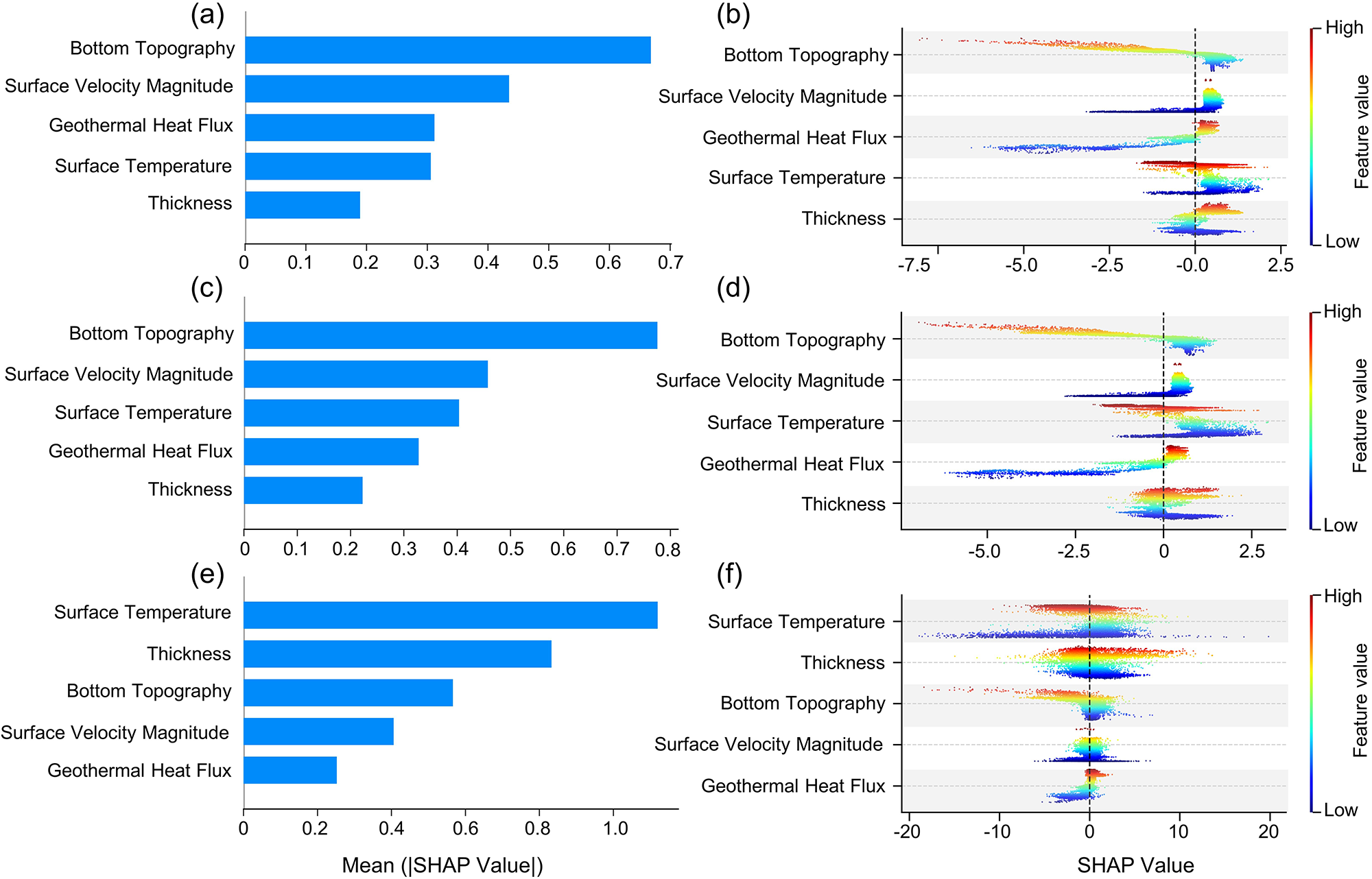
SHAP value analysis from the final RF emulator reveals that the bottom topography is the single most influential predictor of basal temperature, followed by surface ice velocity (Fig. 5a). The distribution of SHAP values (Fig. 5) shows that, generally, bottom topography demonstrates a negative contribution to basal ice temperature, where higher bedrock elevations correspond to lower predicted basal ice temperatures. Conversely, both surface ice velocity and GHF show a positive contribution, meaning higher values in these variables tend to predict warmer basal temperature.
The mean of absolute SHAP values of each contributor (left column) and distribution of SHAP values (right column) in the emulator RF (a, b), XGBoost (c, d) and NN (e, f). The larger the SHAP values magnitude, the larger contribution to the predicted basal ice temperature. A positive/negative SHAP value means that the factor tends to increase/decrease the predicted basal ice temperature. Each cluster of scattered points (N = 23 240) corresponds to the distribution of SHAP values for the specific feature, where the points are vertically jittered slightly around a dotted horizontal line to avoid overlap and facilitate the visualization of data density. We adopt alternating gray-white background shades in the right column to enhance the visual separation between different features.

Figure 5 Long description
The image A showing a horizontal bar chart. Text: Bottom Topography; Surface Velocity Magnitude; Geothermal Heat Flux; Surface Temperature; Thickness. Horizontal axis label: Mean (absolute SHAP Value). Horizontal axis range: 0.0 to 0.7. Bars: Bottom Topography about 0.65; Surface Velocity Magnitude about 0.55; Geothermal Heat Flux about 0.30; Surface Temperature about 0.20; Thickness about 0.10. The image B showing a scatter plot with five horizontal feature rows. Text on rows: Bottom Topography; Surface Velocity Magnitude; Geothermal Heat Flux; Surface Temperature; Thickness. Horizontal axis label: SHAP Value. Horizontal axis range: negative 7.5 to 2.5. Vertical axis label: Feature value. No unit shown. Each feature row contains many points spread along the SHAP Value axis. The image C showing a horizontal bar chart. Text: Bottom Topography; Surface Velocity Magnitude; Surface Temperature; Geothermal Heat Flux; Thickness. Horizontal axis label: Mean (absolute SHAP Value). Horizontal axis range: 0.0 to 0.8. Bars: Bottom Topography about 0.75; Surface Velocity Magnitude about 0.55; Surface Temperature about 0.45; Geothermal Heat Flux about 0.30; Thickness about 0.20. The image D showing a scatter plot with five horizontal feature rows. Text on rows: Bottom Topography; Surface Velocity Magnitude; Surface Temperature; Geothermal Heat Flux; Thickness. Horizontal axis label: SHAP Value. Horizontal axis range: negative 5.0 to 2.5. Vertical axis label: Feature value. No unit shown. Each feature row contains many points spread along the SHAP Value axis. The image E showing a horizontal bar chart. Text: Surface Temperature; Thickness; Bottom Topography; Surface Velocity Magnitude; Geothermal Heat Flux. Horizontal axis label: Mean (absolute SHAP Value). Horizontal axis range: 0.0 to 1.0. Bars: Surface Temperature about 1.0; Thickness about 0.75; Bottom Topography about 0.55; Surface Velocity Magnitude about 0.35; Geothermal Heat Flux about 0.25. The image F showing a scatter plot with five horizontal feature rows. Text on rows: Surface Temperature; Thickness; Bottom Topography; Surface Velocity Magnitude; Geothermal Heat Flux. Horizontal axis label: SHAP Value. Horizontal axis range: negative 20 to 20. Vertical axis label: Feature value. No unit shown. Each feature row contains many points spread along the SHAP Value axis.
These findings are strongly corroborated by the XGBoost emulator. Although it slightly alters the ranking of the less influential variables (swapping surface temperature and GHF), it agrees with the RF emulator that bottom topography and surface ice velocity are the two dominant drivers. Crucially, the physical nature of these relationships (i.e. whether a variable’s contribution is positive or negative) is identical between both tree-based emulators (Fig. 5b and d). It is important to interpret these relative rankings with caution. A lower rank for a variable like ice thickness does not imply it is physically unimportant; rather, it suggests that within the context of our training data, other variables provided stronger predictive power. Interestingly, the NN emulator diverged somewhat from the tree-based emulators, ranking ice thickness as the third most important variable. Despite these differences in ranking, the fundamental physical relationships identified by the NN—such as the negative contribution of bottom topography and the positive contribution of GHF—were consistent with the other emulators. This broad agreement across three different ML architectures provides confidence in the physical realism captured by our emulators.
3.4. Simultaneous prediction of basal ice temperature and melt rate
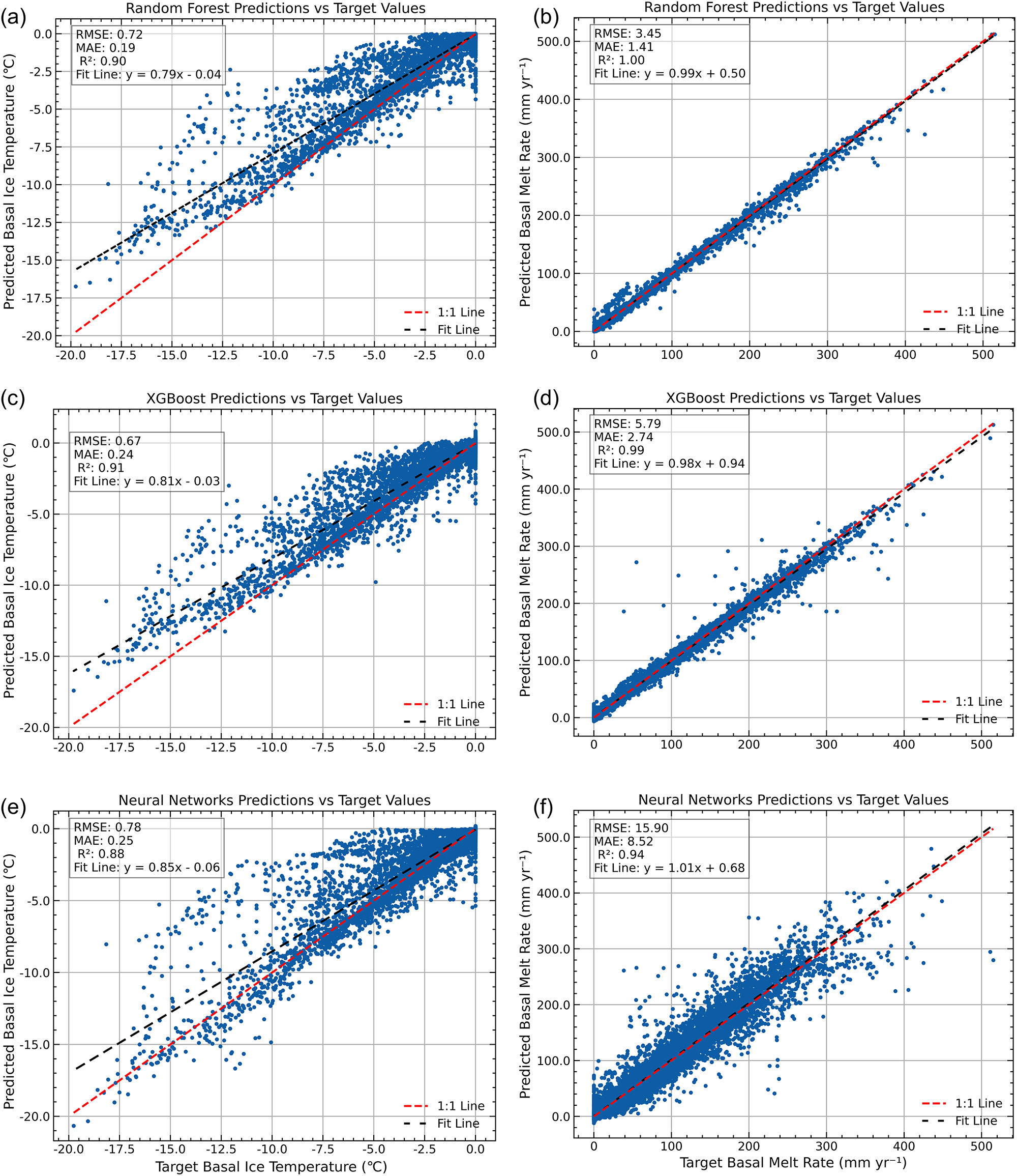
We next assessed the emulators’ capability to perform a more complex task: predicting basal ice temperature and basal melt rate simultaneously from the same set of input variables. The tree-based emulators handled this multi-output challenge exceptionally well. As shown in Fig. 6, both the RF and XGBoost emulators maintained their high accuracy for basal temperature prediction while also delivering accurate predictions for the basal melt rate. For multi-target predictions, we utilized XGBoost’s built-in multi-output regression support. Unlike traditional wrappers that train separate models for each output, this native configuration builds vector-leaf trees, in which each leaf stores a vector of predictions for both basal temperature and melt rate simultaneously. The performance of the NN emulator for temperature prediction shows a minor degradation when it is also tasked with predicting melt rate. This slight trade-off is expected, as the emulator must optimize its internal parameters to minimize the combined prediction error for two distinct variables. SHAP value analysis for the basal melt rate predictions reveals a consistent and physically intuitive driver across all three emulators. Surface ice velocity is identified as the overwhelmingly dominant predictor, with higher velocities consistently corresponding to higher predicted melt rates (Supplementary Fig. S7). This finding aligns with the physical understanding that frictional heat, a key component of basal melt, is directly related to the sliding velocity at the ice-bed interface.
Simultaneous prediction performance of both basal ice temperature and melt rate on the test set of RF emulator (a, b), XGBoost emulator (c, d) and NN emulator (e, f), N = 23 240.

Figure 6 Long description
The image A showing a scatter plot titled Random Forest Predictions vs Target Values. Text block: RMSE: 0.77; MAE: 0.59; R: 0.99; N: 23240; Fit Line: y equals 0.79x minus 0.04. Horizontal axis label: Target Basal Ice Temperature (degrees C). Horizontal axis range: negative 20.0 to 0.0. Vertical axis label: Predicted Basal Ice Temperature (degrees C). Vertical axis range: negative 20.0 to 0.0. Legend text: 1:1 Line; Fit Line. The image B showing a scatter plot titled Random Forest Predictions vs Target Values. Text block: RMSE: 3.45; MAE: 1.44; R: 1.00; N: 23240; Fit Line: y equals 0.99x plus 0.50. Horizontal axis label: Target Basal Melt Rate (mm yr superscript -1). Horizontal axis range: 0 to 450. Vertical axis label: Predicted Basal Melt Rate (mm yr superscript -1). Vertical axis range: 0 to 450. Legend text: 1:1 Line; Fit Line. The image C showing a scatter plot titled XGBoost Predictions vs Target Values. Text block: RMSE: 0.67; MAE: 0.49; R: 0.99; N: 23240; Fit Line: y equals 0.81x minus 0.03. Horizontal axis label: Target Basal Ice Temperature (degrees C). Horizontal axis range: negative 20.0 to 0.0. Vertical axis label: Predicted Basal Ice Temperature (degrees C). Vertical axis range: negative 20.0 to 0.0. Legend text: 1:1 Line; Fit Line. The image D showing a scatter plot titled XGBoost Predictions vs Target Values. Text block: RMSE: 5.79; MAE: 2.70; R: 0.99; N: 23240; Fit Line: y equals 0.98x plus 0.94. Horizontal axis label: Target Basal Melt Rate (mm yr superscript -1). Horizontal axis range: 0 to 450. Vertical axis label: Predicted Basal Melt Rate (mm yr superscript -1). Vertical axis range: 0 to 450. Legend text: 1:1 Line; Fit Line. The image E showing a scatter plot titled Neural Networks Predictions vs Target Values. Text block: RMSE: 0.74; MAE: 0.55; R: 0.98; N: 23240; Fit Line: y equals 0.85x minus 0.03. Horizontal axis label: Target Basal Ice Temperature (degrees C). Horizontal axis range: negative 20.0 to 0.0. Vertical axis label: Predicted Basal Ice Temperature (degrees C). Vertical axis range: negative 20.0 to 0.0. Legend text: 1:1 Line; Fit Line. The image F showing a scatter plot titled Neural Networks Predictions vs Target Values. Text block: RMSE: 15.90; MAE: 8.52; R: 0.94; N: 23240; Fit Line: y equals 1.01x plus 0.68. Horizontal axis label: Target Basal Melt Rate (mm yr superscript -1). Horizontal axis range: 0 to 450. Vertical axis label: Predicted Basal Melt Rate (mm yr superscript -1). Vertical axis range: 0 to 450. Legend text: 1:1 Line; Fit Line.
4. Discussion
In our final prediction experiments, we evaluate the performance of three ML emulators using the independent test set that includes the Purucker (Reference Purucker2012) and Martos and others (Reference Martos, Catalán, Jordan, Golynsky, Golynsky, Eagles and Vaughan2017) datasets. Our results confirm the potential of ML emulators to efficiently reproduce computationally expensive ice-sheet simulations. The XGBoost emulator yields a marginally superior performance, but all three nonlinear emulators (XGBoost, RF and NN) substantially outperform the baseline linear regression. This finding strongly suggests that the relationship between glaciological inputs and basal temperature is fundamentally nonlinear, making sophisticated, data-driven approaches essential for accurate prediction. The results align with the conclusions of Anilkumar and others (Reference Anilkumar, Bharti, Chutia and Aggarwal2023), who similarly advocated for complex emulators in glacier mass balance prediction.
A closer analysis of emulator errors reveals a key challenge for any data-driven emulator in the geosciences: extrapolation. All emulators, whether linear or ML-based, show some overestimation on the test set, as evidenced by the distribution of fitted lines compared to the 1:1 line (Fig. 2). Upon splitting the test set into individual datasets, we observe that the overestimated predictions predominantly originated from the Purucker (Reference Purucker2012) dataset (Fig. 3a and Supplementary Figs. S4a and S5a). The Purucker (Reference Purucker2012) dataset includes basal ice temperatures lower than those in the training data, which have temperatures ranging from −17.11°C to 0°C, whereas the minimum temperature in the Purucker (Reference Purucker2012) dataset is −19.7°C. This discrepancy likely contributes to the overestimation of basal ice temperature by the emulator. The emulators, having never seen such cold examples, struggle to predict accurately outside their training domain. This highlights a limitation not of the emulators themselves, but of the representativeness of the training data.
Furthermore, the predictive challenge is compounded by a data imbalance issue. The basal thermal state of Totten Glacier is highly skewed, with a large fraction of the domain at or near the pressure-melting point. This skewed distribution limits the ability of data-driven emulators to effectively learn from lower-temperature samples (Ribeiro and Moniz, Reference Ribeiro and Moniz2020; Dolar and others, Reference Dolar, Chen and Chen2025). While applying weighted balancing techniques to different samples may address this issue, such an approach may not universally improve prediction performance across all scenarios. Additionally, the linear regression model emulator demonstrates poor performance on both the training and test datasets. This underperformance could be attributed to two primary factors: (1) the absence of a linear relationship between input features and basal ice temperature; (2) the skewed distribution of basal ice temperatures in Totten Glacier violates the linear regression model’s assumption of normality. These combined factors likely contribute to its suboptimal predictive capabilities.
Our analysis of training set size reveals that the RF emulator was the most robust when data were limited, consistently outperforming the other emulators with small training sets. This accords with existing literature suggesting that RF’s bagging approach is highly resistant to overfitting, making it a reliable choice when data are scarce (Moghaddam and others, Reference Moghaddam2020; Ramezan and others, Reference Ramezan, Warner, Maxwell and Price2021). Perhaps more importantly, we found that emulator performance is sensitive not just to the quantity of training data, but to its quality and diversity. The inclusion of the An and others (Reference An2015) simulation consistently improved the performance of all emulators. As shown in Fig. 4 and Supplementary Fig. S6, this dataset provides a uniquely comprehensive sample of the glacier’s thermal state, spanning both warm and cold regimes. Its inclusion likely provides the emulator with a more complete and representative picture of the system’s physics. In contrast, the inclusion of the Purucker (Reference Purucker2012) dataset decreased the R2 scores for RF and XGBoost in the test set. This suggests that basal ice temperature data from this dataset—particularly in the southwestern region of Totten Glacier—exhibit poor alignment with the other datasets, likely attributable to its lower simulated ice temperatures (Huang and others, Reference Huang, Zhao, Wolovick, Ma and Moore2024). This underscores that for developing robust ML emulators, selecting a diverse set of training simulations that covers the full range of expected behaviors is as important as the ML architecture itself.
While all three ML emulators achieve high predictive accuracy, their internal mechanisms differ, leading to a divergence in what they appear to have learned about the glacier’s physics. Tree-based ensemble emulators, whether they employ the bagging strategy of RF or the boosting strategy of XGBoost, are fundamentally built on decision trees. This architecture excels at learning piecewise, non-linear relationships, making it adept at capturing phenomena governed by thresholds. In contrast, NN learns through a series of linear transformations and nonlinear activation functions. While NNs are universal function approximators, the structure inherently favors learning smooth, continuous functions. This architectural difference is reflected in the feature importance results from our SHAP analysis. For both the RF and XGBoost emulators, bottom topography emerges as the dominant factor, exhibiting a consistent negative contribution to basal ice temperature. This relationship is physically grounded: given the generally smooth glacier surface, higher basal topography corresponds to thinner overlying ice. Thinner ice provides less insulation from cold surface temperatures, leading to a cooler ice base (Fig. 6). Bottom topography demonstrates a greater influence than ice thickness in RF and XGBoost emulators, but a smaller influence than ice thickness in the NN emulator. Consistent across all emulators, GHF exerts a positive contribution to basal temperature. Similarly, surface ice speed is an important predictor, particularly in the RF and XGBoost emulators. Its positive contribution is well-understood: higher surface velocities are often associated with greater heat dissipation from ice deformation and sliding, which can contribute to higher basal temperatures.
The feature rankings reveal that the emulators have developed different physical sensitivities. The tree emulators (RF and XGBoost) prioritize features driving local, dynamic heat production at the ice-bed interface: basal topography (which influences pressure and stress concentrations) and ice velocity (which generates friction). Conversely, the NN assigns greater importance to large-scale predictor variables such as surface temperature and ice thickness, which are associated with broad thermal structure in the modeled outputs. This suggests that the NN appears to capture a lower-complexity statistical mapping that is more strongly influenced by globally predictive variables. In contrast, the tree-based emulators appear to rely more strongly on predictors associated with local variability, leading to a different but still physically interpretable predictor ranking. Interestingly, the positive and negative contributions of the variables to basal ice temperature are largely consistent, although there are differences in the ranking of the most influential variables. It is noted that some of the predictor variables are correlated, and this can influence SHAP-based attribution by redistributing importance among related features. For example, geometric variables such as bedrock elevation and ice thickness are not fully independent, so part of the importance attributed to one variable may reflect shared information with another correlated predictor. In the present study, the differing feature sensitivities of the three emulator types suggest that relying on a single pointwise emulator may provide only a partial view of the modeled relationships. For the specific model classes considered here, comparing multiple architectures can therefore provide a more balanced interpretation when combined with domain expertise.
We further demonstrate that ML emulators can emulate the simultaneous prediction of both basal temperature and melt rate, like ice-sheet simulations. This is not merely a technical exercise; it serves a vital scientific purpose. Totten Glacier has extensive warm-bed areas where the basal ice temperature reaches the pressure-melting point. In contrast, the basal melting rate varies significantly when the basal ice temperature reaches pressure-melting point, which can thus demonstrate the prediction performance of the ML emulator across the warm-bed areas to a certain extent. From the simultaneous prediction results, both RF and XGBoost emulators accurately predict basal melting rate without significantly compromising basal ice temperature predictions. This is due to the tree-based nature of these emulators, which can handle multiple targets simultaneously. This near-perfect agreement is also physically consistent with the expected energy budget: melt rates of order 100 mm yr−1, as seen in Fig. 6, require latent heat fluxes of approximately 1 W m−2, which are at least an order of magnitude larger than typical GHF values. This suggests that, for these relatively high melt rates, variations among GHF datasets make only a secondary contribution compared with dynamical heat sources such as basal friction and internal deformation. Thus, variations among the geothermal datasets have only a minor effect on the simulated basal melting rates. The two target variables were standardized before training in the simultaneous-prediction experiments. The NN’s temperature predictions are slightly degraded in the simultaneous-prediction setting, indicating that greater care is required when training a shared model for multiple outputs. In the present implementation, we set the loss weighting ratio of the two target variables to 1:2 (basal temperature to melt rate), which is a reasonable empirical choice. This configuration produced acceptable results, but it should not be regarded as uniquely optimal, and further improvements may be possible using more advanced multitask training strategies. We nevertheless retained the shared multi-output architecture because our aim was to test whether a single emulator could simultaneously reproduce multiple basal thermal quantities generated together by the underlying ice-sheet model, and to potentially capture their statistical interdependencies. In the simultaneous prediction emulator, the surface ice velocity is the main factor affecting the basal melting rate, which is reflected in the emulator’s SHAP calculation (Supplementary Fig. S7). This is because the surface ice velocity and basal ice velocity are often positively correlated, and higher basal ice velocity will produce higher frictional heat, which is the primary driver of basal melting in Totten Glacier.
The transferability of these emulators remains an important caveat. The emulators in this study learn a specific mapping from a small set of steady-state variables to basal temperatures under a specific model configuration (Huang and others, Reference Huang, Zhao, Wolovick, Ma and Moore2024). They cannot be assumed to be directly applicable to other glacier systems. Furthermore, the emulators are constructed in a pointwise manner without incorporating spatial context. Consequently, the emulators are best interpreted as learning local statistical relationships within Totten Glacier, and are unlikely to represent processes governed by long-range physical connections. As an additional sensitivity analysis, we performed a spatial-block validation experiment to assess the potential influence of spatial autocorrelation and nonuniform mesh density on node-wise performance metrics. This analysis was conducted using only the six development GHF scenarios, while the Purucker (Reference Purucker2012) and Martos and others (Reference Martos, Catalán, Jordan, Golynsky, Golynsky, Eagles and Vaughan2017) scenarios remained reserved for the main withheld-GHF scenario evaluation. Spatial blocks were generated from the common mesh-node coordinates and grouped into five spatial cross-validation folds. This spatial-block validation was not used for hyperparameter tuning or model selection, but served as a conservative sensitivity test of model generalization across both geographic space and associated feature-space regimes, that is, spatially distinct combinations of physical conditions. The spatial-block validation produced lower but still moderate predictive performance compared with random node-based validation, with R 2 values of approximately 0.7 for multiple ML emulators (Supplementary Fig. S8). This result supports the interpretation that the emulators show reduced generalization across spatially distinct physical regimes than across randomly mixed nodes. Nevertheless, the retained performance under spatial-block validation suggests that the emulators capture meaningful local statistical relationships in the input variables. These results do not alter the main model comparison, which is based on the independent withheld GHF scenarios, but provide a more conservative assessment of spatial generalization.
This work demonstrates the potential of ML emulators in glaciology but also highlights areas for future refinement. Future work should also explore techniques to address the data imbalance issue, such as applying different weights in the loss function to force the emulator to pay more attention to the rare, cold-based samples. For multi-output prediction with NNs, further investigation into optimal loss function weighting is warranted. By addressing these limitations, future ML emulators can become more reliable tools that mitigate the high computational costs and other limitations associated with ice-sheet dynamic models.
5. Conclusion
In this study, we demonstrate that ML can create computationally efficient and accurate emulators of a sophisticated, full-Stokes ice dynamics model for predicting basal ice temperature across the Totten Glacier basin. All three ML emulators (RF, XGBoost and NN) substantially outperform a traditional linear regression, confirming that the physical relationships governing basal temperature are inherently complex and nonlinear. The XGBoost emulator yields the highest overall accuracy (R 2 ≈ 0.91). The emulators identify physically meaningful drivers. The SHAP analysis identifies basal topography as the dominant control on basal ice temperature and surface ice velocity as the primary driver of basal melt rate. We establish that a minimum of five diverse numerical simulations is sufficient to train a robust emulator that closely reproduces the basal ice temperature simulated by the ice dynamics model for Totten Glacier. Furthermore, the emulators can simultaneously predict basal temperature and melt rate, providing a diagnostic for warm-based ice where temperature alone is an insufficient metric. Our interpretability analysis reveals that the tree-based emulators (RF and XGBoost) capture localized statistical relationships by prioritizing local, dynamic features at the ice-bed interface, such as friction (proxied by surface velocity) and insulation effects from basal topography. In contrast, the NN acts like a lower-complexity statistical emulator, prioritizing globally predictive inputs like surface temperature and overall ice thickness. This finding underscores that a multi-emulator approach can offer a more balanced physical interpretation for the specific model classes considered here. The primary implication of this work is that the ML emulation framework provides a powerful and computationally inexpensive complementary approach to running large, computationally prohibitive ensembles of numerical simulations for sensitivity analysis and uncertainty quantification. While the trained emulators presented here are specific to Totten Glacier, the methodology itself is transferable to other glacial systems provided the models are retrained and reevaluated. It offers a promising pathway for conducting sensitivity analyses and uncertainty quantification for complex glaciological systems within a diagnostic framework. Ultimately, we emphasize that while the superior predictive performance of ML methods can help mitigate the high computational cost of numerical simulations, their interpretation must be combined with deep domain expertise to produce robust and physically meaningful scientific insights.
Supplementary material
The supplementary material for this article can be found at https://doi.org/10.1017/jog.2026.10170.
Data availability statement
MEaSUREs BedMachine Antarctica, version 2, is available at https://doi.org/10.5067/E1QL9HFQ7A8M (Morlighem and others, Reference Morlighem2020). MEaSUREs InSAR-Based Antarctic Ice Velocity Map, version 2, is available at https://doi.org/10.5067/D7GK8F5J8M8R (Rignot and others, Reference Rignot, Mouginot and Scheuchl2017). MEaSUREs Antarctic Boundaries for IPY 2007–2009 from Satellite Radar, version 2, is available at https://doi.org/10.5067/AXE4121732AD (Mouginot and others, 2017). ALBMAP v1 and the GHF dataset of Shapiro and Ritzwoller (Reference Shapiro and Ritzwoller2004) are available at https://doi.org/10.1594/PANGAEA.734145 (Le Brocq, Payne, Vieli, 2010b). The GHF dataset of An and others (Reference An2015) is available at http://www.seismolab.org/model/antarctica/lithosphere/AN1-HF.tar.gz (last access: 11 April 2023). The GHF dataset of Shen and others (Reference Shen, Wiens, Lloyd and Nyblade2020) is available at https://sites.google.com/view/weisen/research-products?authuser=0 (last access: 11 April 2023). The GHF dataset of Reference Martos, Catalán, Jordan, Golynsky, Golynsky, Eagles and VaughanMartos and others (2017) is available at https://doi.org/10.1594/PANGAEA.882503. The GHF dataset of Purucker (Reference Purucker2012) is available at https://core2.gsfc.nasa.gov/research/purucker/heatflux_mf7_foxmaule05.txt (last access: 11 April 2023).
Funding statement
This work was supported by the National Natural Science Foundation of China (grant no. 42576280) and the Finnish Academy (grant no. 355572).
Competing interests
The corresponding author has declared that none of the authors have any competing interests.


 Open access

