

Introduction
Sea ice is a key element in earth's climate system, it has an impact on the heat and moisture transfer between the ocean and the atmosphere and influences the global albedo (Ebert and Curry, Reference Ebert and Curry1993). Sea ice contains, unlike freshwater ice, brine in pore networks and inclusions. Often termed ‘brine channels’, these are the habitat to a whole ecosystem crucial for the arctic food web (Legendre and others, Reference Legendre, Ackley, Dieckmann, Gulliksen and Horner1992). As the interest in exploring natural resources and shipping traffic in the Arctic is increasing (Peters and others, Reference Peters, Nilssen, Lindholt, Eide and Glomsrød2011), sea ice becomes an engineering challenge (Schwarz and Weeks, Reference Schwarz and Weeks1977). Human activities bear the risk of increased marine pollution and oil spills. The sea-ice porous space can act as a buffer (Petrich and others, Reference Petrich, Karlsson and Eicken2013; Salomon and others, Reference Salomon, Arntsen, Phuong, Maus and O'Sadnick2017; Desmond and others, Reference Desmond, Crabeck, Lemes, Harasyn and Mansoori2021). Hence, physical, optical and mechanical characteristics of sea ice, relevant to its geophysical, biological and engineering properties, are strongly linked to its microstructure.
Early studies on sea-ice structure were mainly dominated by two-dimensional (2-D) macroscopic descriptions (cm-mm scale) of either vertical or horizontal sections. Destructive preparation of thin- or thick sections was necessary to allow studies on sea-ice structure. Based on such sections, Lake and Lewis (Reference Lake and Lewis1970) illustrated the overall 3-D patterns of brine channels systems. Since then there have been a couple of microstructure studies based on optical thin section analysis summarised in Weeks (Reference Weeks2010) and Shokr and Sinha (Reference Shokr and Sinha2015). Extended thin section analysis by electron microscope observation has resulted in detailed 2-D views of single brine inclusions (Sinha, Reference Sinha1977). 3-D insights and the application of X-ray computed tomography (CT) to sea-ice samples were first given by Kawamura (Reference Kawamura1988). This study allowed for the first time non-destructive observation of sea ice, with a resolution of 2 mm. Since then, advances in technology have allowed examination at much higher resolution with micro-X-ray CT (μ-CT). Applying μ-CT on laboratory sea ice has advanced understanding in the field. Golden and others (Reference Golden, Eicken, Heaton, Miner and Pringle2007) and Pringle and others (Reference Pringle, Miner, Eicken and Golden2009) investigated brine inclusions within sea ice, its connectivity and permeability supporting the percolation theory. Crabeck and others (Reference Crabeck, Galley, Delille, Else and Geilfus2016) conducted studies on the spatial distribution of gas bubbles and gas transport within sea ice. Insights into pollutant distribution within sea ice on the example of crude oil were given by Oggier and others (Reference Oggier, Eicken, Wilkinson, Petrich and O'Sadnick2019) and Petrich and others (Reference Petrich, O'Sadnick, Brekke, Myrnes and Maus2019). Eicken and others (Reference Eicken, Bock, Wittig, Miller and Poertner2000) investigated microstructure and thermal evolution of brine inclusions with magnetic resonance imaging on laboratory and natural grown sea ice. The first μ-CT-images of field collected sea ice were published in 2009 (Maus and others, Reference Maus, Huthwelker, Enzmann, Miedaner and Marone2009; Obbard and others, Reference Obbard, Troderman and Baker2009; Lieb-Lappen and others, Reference Lieb-Lappen, Golden and Obbard2017). To diminish the likelihood of changing pore structure during transport and storage from changing temperatures, Maus and others (Reference Maus, Huthwelker, Enzmann, Miedaner and Marone2009) proposed a method that had earlier been used to obtain cast samples of the sea-ice pore space (Freitag, Reference Freitag1999; Weissenberger and others, Reference Weissenberger, Dieckmann, Gradinger and Spindler1992). Prior to μ-CT imaging, samples were transported close to their in situ temperature to the lab and were centrifuged. Removal of the brine allows that samples can be further stored and transported at sub-eutectic temperatures without altering the pore structure to reveal insights into pore size distribution and permeability of sea ice. These data were used to model oil entrapment in ice (Maus and others, Reference Maus, Huthwelker, Enzmann, Miedaner and Marone2009, Reference Maus, Leisinger, Matzl, Schneebeli and Wiegmann2013, Reference Maus, Becker, Leisinger, Matzl and Schneebeli2015). This paper aims to investigate the sea-ice pore space, which is defined by its brine networks and air inclusions on a microscale. The physical parameters including sea-ice temperature, salinity, density, porosity, pore size, throat size and pore number per area were studied. Sea-ice density and salinity measurement based on CT-microstructural observation are compared with hydrostatical density evaluations and salinity determined from conductivity.
Methods
Study site
Fieldwork location was Sveasundet, south of Sveagruva in Van Mijenfjorden, Spitsbergen (77°53′13.0″ N 16°44′23.1″ E) (Fig. 1). From 16 March until 23 April 2016, eight site visits were conducted.
Field work location: Sveasundet, south of Sveagruva in Van Mijenfjorden, Spitsbergen (77°53′13.0″ N 16°44′23.1″ E).

Field set-up
Field site preparation took place on 16 and 17 March 2017. Two sea-ice temperature profiles were logged throughout the field campaign, each with a set of six type T thermocouples. Registered sea-ice temperature was logged every 5 s with USB-5104 4-channel thermocouple loggers from Measurement Computing with a time accuracy of ±1 min per month at 25°C. Prior to the installation of the sea-ice temperature devices, thermocouples were mounted with a spacing of 10 cm inside a paperboard tube with an inner diameter of 7.8 cm and an outer diameter of 8.2 cm. An ice core with a diameter of 7.2 cm was drilled with a Kovacs 1 m core barrel and fitted into the paperboard tube. The tube equipped with thermocouples and filled with the ice core was re-positioned to its in situ position. The thermocouples were oriented such that one set of thermocouples was facing to the south and the other set was facing to the north. Unfortunately, the thermocouples started giving erroneous results after our second visit, probably due to a moisture problem.
A temperature sensor (SBE 56, Sea bird Scientific) with a resolution of 0.0001°C and an accuracy of ± 0.002°C (range: − 5 to + 35°C) was installed 1.2 m below the ice surface to register ocean temperatures. The ocean temperature was logged in an interval of 2 min.
Snow depth above the ice cover was measured at several locations on each field day with a commercial benchmark with a resolution of 1 mm. The snow temperature was measured at the surface as well as the slush-ice interface with a portable thermometer (HI 93510 from Hanna Instruments, accuracy: 0.4°C, resolution: 0.1°C).
After the installation of temperature loggers, two salinity cores, two temperature cores, two cores for microstructure analysis and one for density determination were drilled. This coring regime was repeated on 30 March, 06, 12 and 23 April.
All cores except cores from 30 March were drilled with a core barrel of 7.2 cm in diameter. Cores from 30 March were drilled with a core barrel of 12 cm in diameter, due to technical issues with the core barrel of 7.2 cm in diameter. Bulk salinity, temperature and density cores were drilled next to each other. Temperature cores were extracted one by one and measured immediately after coring. The temperature was measured with a portable thermometer (HI 93510 from Hanna Instruments) from bottom to top every 2.5 cm. Bulk salinity cores were measured in length and sub-sampled from bottom to top in 2.5 cm steps. Subsamples were packed into watertight plastic containers and transported back to the laboratory in Longyearbyen. Density cores were measured in length, sub-sampled to a height of 5 cm, packed into plastic containers and transported at ambient temperature in an upright position to the laboratory.
Microstructure cores were measured in length and sub-sampled to a height of 2.5 cm from bottom to top. The subsamples were packed in conical plastic boxes to avoid the sample touching the floor of the container and transported in an upright postion in active cooling boxes (WAECO T22,T32 and WAECO Cool Freeze CDF35) as close as possible to their in situ temperature to the UNIS laboratories.
Laboratory set up and methods
Bulk salinity (S ice) of melted samples from the field was measured. We used a HI 98 188 conductivity/salinity meter from Hanna instruments to determine the salinity measured in practical salinity unit (psu). Sea-ice density (ρ) was determined by hydrostatic weighing in paraffin (Fritidsparafin by Wilhelmsen Chemicals), based on Archimedes’ law (Kulyakhtin and others, Reference Kulyakhtin, Kulyakhtin, Løset, Chung, Langen, Kokkinis and Wang2013; Pustogvar and Kulyakhtin, Reference Pustogvar and Kulyakhtin2016).

Ice samples were weighed in air (M air) and submerged in paraffin (M par) using a Kern KB 2000-2NM scale (resolution 0.01 g and accuracy 0.1 g). The paraffin density (ρ par) was determined with an aerometer (resolution: 1 kg m−3) to calculate the sea-ice density (Eqn (1)). Density measurements were performed in a cold lab at − 15°C, except for the cores from 17 and 30 March, which were measured at − 2.7°C. Air porosity from density was determined using equations by Cox and Weeks (Reference Cox and Weeks1982), with density values from hydrostatic weighing and measured bulk salinity.
Samples for microstructure analysis were first weighed using a scale from PCE Group, BT 2000, and then reduced utilising a core barrel to a diameter of 4 cm. The cut-off from drilling was collected after this step. Afterwards, the reduced sample was centrifuged for 10 min at a set temperature of − 3°C and 900 revolutions per minute, corresponding to 40 G in a cooled centrifuger (Minifuge Heraeus Christ). The centrifuged samples were packed in plastic bags, stored at − 15°C and transported at this temperature to the Norwegian University of Technology (NTNU). Samples were stored at NTNU for 11 months at − 15°C before further investigations. Centrifuging of ice samples makes it feasible to transport and investigate the microstructure of sea-ice samples, close to in situ conditions, without uncontrolled loss of brine and preserving the sea-ice microstructure. The amount and salinity of dripped brine (S bdrip) during transport was determined, as well as the amount and salinity of the cut-off (S rest) and the centrifuged brine (S bcent). The salinity of the centrifuged microstructure samples (S cent) was measured after μ-CT analysis at NTNU.
Micro computed-tomography imaging and post imaging processing
We conducted 3-D X-ray micro-tomographic imaging at the Norwegian Centre for X-ray Diffraction, Scattering and Imaging (RECX), NTNU, with a XT H 225 ST micro-CT system from Nikon Metrology NV, equipped with a Perkin Elmer 1620 flat panel detector with a 2048 × 2018 pixel field of view. Image acquisition was performed with a current source of 250 μA, an acceleration voltage of 150 kV and a Wolfram target. Scans were performed with 3142 rotation per 360° and an exposure time of 708.00 ms. The field of view (FOV) was 50 mm and corresponds to a pixel size of 25 μm. Samples were placed in an alumina sample holder with 1 mm wall thickness. The top and bottom temperature of the sample holder was controlled by a self-assembled cooling system, based on thermoelectric assemblies (www.lairdtech.com). The temperature during scanning was set to − 15°C, the same temperature as during transport and storage. Nikon Metrology XT Software was used for reconstruction of the datasets. During reconstruction, we applied a beam hardening correction. Data were stored as 16-bit grey value stacks.
Data stacks were first processed in Image J. First, we cropped the cross-sections into a FOV of 1150 × 1150 pixel and cut to an average vertical extend of 400–650 slices. Images were then filtered using a combination of a Median filter (radius: 2 voxel) and a Gaussian filter (radius: 1.5 voxel), where a voxel is a 3-D pixel. In the next step, images are segmented into three classes: ice, air or brine. Otsu's algorithm (Otsu, Reference Otsu1979; Maus and others, Reference Maus, Becker, Leisinger, Matzl and Schneebeli2015) was applied for differentiation between the air and ice signal. This was done in a semi-automatic manner. Therefore, five sub-areas in a 2-D slice were chosen. Each area contained a similar fraction of ice and air, on which the threshold based on Otsu's algorithm was computed. The mean of these thresholds was selected for air segmentation. For segmentation of brine from ice, the Triangle algorithm (Zack and others, Reference Zack, Rogers and Latt1977) was applied. The Triangle algorithm was chosen for brine segmentation, as Otsu's algorithm gave brine volumes that were too high (Hullar and Anastasio, Reference Hullar and Anastasio2016). First, the threshold was estimated for 41 samples, where in each of the samples five subregions containing a similar amount of brine and ice, without containing air, were investigated. Based on these 41 samples, it was found that the ratio of this threshold and the histogram peak corresponding to ice was 1.13 (±0.03). In the second step, brine segmentation was based on a threshold 1.13 times the ice histogram peak (Fig. 2).
Filtered grey scale CT-scans for (a) a sample with a small number of macro pores and (c) a large number of macro pores. Filtered data are segmented into air (blue), brine (green) and ice (grey). The histograms in the middle show the linear grey value distribution in black and the logarithmic distribution in grey with a significant ice peak.

Pore space analysis
Bulk properties: porosity, salinity and density
We used the software GeoDict 2018 and 2019 (Linden and others, Reference Linden, Cheng and Wiegmann2018) to determine different porosity metrics of the pore space, salinity and density. We are interested in the following porosity metrics in situ:
-
ϕ b = brine porosity
-
ϕ bopen = open brine porosity
-
ϕ bclosed = closed brine porosity
-
ϕ bcon = connected brine porosity
-
ϕ air = air porosity
The CT output is the segmentation into air and brine:
-
$\phi ^{{\rm CT}}_{{\rm brine}}$
 = brine and solid salt porosity in CT image (residual)
 -
$\phi ^{{\rm CT}}_{{\rm air}}$
= air porosity in CT image


The air porosity from the CT output consists of centrifuged brine pores and disconnected air pores. Open air pores might have existed, but are further considered as open brine pores. It can be further geometrically analysed by taking directional information into account (see Fig. 3 for illustration):
-
$\phi ^{{\rm CT}}_{{\rm air\ closed}}$
= closed air porosity in CT image -
$\phi ^{{\rm CT}}_{{\rm air\ open}}$
= open air porosity in CT image -
$\phi ^{{\rm CT}}_{{\rm air\ con}}$
= vertically connected air porosity in CT image


Classification of pores under in situ conditions after sampling transport centrifuging and CT-imaging and after CT-image analysis.

In Geodict, the fractions of open and closed pores can be determined with respect to the six sides of a 3-D image. Where the x-axis (±) and the y-axis (±) do describe the horizontal plane and the z-axis (±) specifies the vertical position in the sample. The open porosity $\phi ^{{\rm CT}}_{{\rm airopen}}$ contains all air pores connected to one of the sample surfaces in any Cartesian direction. A closed pore is considered to be isolated and unreachable from the surfaces. GeoDict does not distinguish connected pores. In order to calculate the connected pore fraction we looked into the open pore space from different intrusion directions: z + (upper surface); z − (lower surface) and z ± (upper and lower surface). The connected pore space can be calculated with the above described metrics as in Eqn (2). Firstly, pores opened to z + and z − direction are counted, the sum of these pores takes all opened pores into account. Since some of the opened pores are counted twice, as they were reached from both z + and z − directions, pores in z + − direction need to be subtracted in a second step in order to get the true number of connected pores. For the example given in Figure 3, two air pores are reached from z +, three pores are opened towards z −, and four pores are opened in z + − direction. Applying Eqn 2 on this example results in one connected pore. At this point, it should be noted that the connected porosity is a subset of the open porosity.

Air pores defined in this way are illustrated in Figure 3. Note that we do not divide the brine porosity, $\phi ^{{\rm CT}}_{{\rm brine}}$ , into open and closed pores. In general, this could be useful to further refine the fraction of closed brine pores that may have been cut and emptied by centrifuging and thus resulted in open air pores. However, the open fraction was found to account for just a few per cent of residual brine and will not be considered here. Figure 3 illustrates how these CT-based porosity metrics are related to in situ metrics. Formally, we use the following relations:
$\phi '_{{\rm bopen}} = \phi ^{{\rm CT}}_{{\rm airopen}}$
$\phi '_{{\rm bcon}} = \phi ^{{\rm CT}}_{{\rm aircon}}$
$\phi '_{{\rm air}} = \phi ^{{\rm CT}}_{{\rm airclosed}}$
$\phi '_{{\rm bclosed}} = f( T,\; T_{{\rm CT}}\ \phi ^{{\rm CT}}_{{\rm brine}}$
)-
ϕ′b = ϕ′bopen + ϕ′bclosed,


where the prime denotes CT-image derived in situ porosities. Hence, pores classified as $\phi ^{{\rm CT}}_{{\rm airopen}}$ $\simeq$
 ϕ′bopen in the CT image are identified with pores that were brine filled and open at in situ conditions and emptied by centrifuging. Closed air pores $\phi ^{{\rm CT}}_{{\rm airclosed}}$ $\simeq$
 ϕ′air and connected brine pores $\phi ^{{\rm CT}}_{{\rm aircon}}$ $\simeq$
 ϕ′bcon are directly identified in the CT images. The brine and solid salt porosity observed in the CT, $\phi ^{{\rm CT}}_{{\rm brine}}$
 , is identified with the disconnected brine and salt that could not be centrifuged. However, as CT imaging was performed at lower temperature (T CT) than the in situ temperature (T) one needs to convert the closed brine fraction ϕ′bclosed by a factor f(T, T CT) to a higher temperature. We use the brine volume dependence from Cox and Weeks (Reference Cox and Weeks1982, Eqn (6)), or f = F1(T CT)/F1(T), to obtain this conversion factor with a small correction: as the conversion is between brine volumina, while the CT imaged brine porosity also contains solid salts, we divide f by 1.031 (F SS) to account for this effect of solid salt volume at T CT = −15°C.
Based on these porosity determinations, the CT-based bulk salinity in psu is obtained:

where ρ b and S b are the brine density and brine salinity at temperature T. Furthermore, the ϕ′b and ϕ′air observations were used to estimate the density. First the ϕ′bopen fraction needed to be converted from higher centrifuging temperature (T cent) to lower T CT. We used the brine volume dependence as described above to estimate the brine volume correction. In the density calculations based on CT measurements, the solid salt fraction in ϕ′bclosed was calculated following Cox and Weeks (Reference Cox and Weeks1982, Eqn (8)) at − 15°C.

Since the solid salt fraction is not resolved in the CT-scans, a factor F SS of 1.031 was applied to calculate the solid salt fraction from the volume brine fraction at − 15°C (Eqn (4)). c gives the phase relation between brine and the solid salt mass in brine in dependence of the temperature following Cox and Weeks (Reference Cox and Weeks1982, Table 1). ρ b and ρ ss are the brine density and solid salt density at temperature T CT.

Field activities

The bulk density was calculated using Eqn (5) at − 15°C, except for the cores from 17 and 30 March, which were performed at − 2.7°C.
Pore sizes
Two characteristic length scales are determined for the pore space:
(1) The pore size distribution (granulometry) (Fig. 18b) is determined by fitting spheres of different sizes into every single point of the pore volume. A point is classified by the diameter of the largest sphere that can be fitted in the pore around it. This frequency of sphere diameters is then binned into classes with 1 voxel (25 μm) bin size. Such a pore size distribution is determined for the pore space classified as closed and open air and brine, corresponding to ϕ′air, ϕ′bopen and ϕ′bclosed, respectively.
(2) The throat size distribution (porosimetry) (Fig. 18c) is not only based on the pore sizes alone, but also considers the connectivity of the pore space to the surfaces. In contrast to the pore size distribution, spheres are injected from the surfaces, and any point is classified by the largest sphere that can reach it via any path. For example, a larger pore that is reached via a bottle neck would be assigned the size of the bottle neck. Porosimetry was determined by considering injections from all sample surfaces and binned into classes with 1 voxel (25 μm) bin size. The approach is comparable to laboratory tests known as Mercury Intrusion Porosimetry (MIP) or Liquid Extrusion Porosimetry (LEP), yet it is a virtual experiment. Using MIP and LEP, a non-wetting fluid or gas is pressed through the pore space while measuring the absorbed volume and the applied pressure. It has recently been applied to analyse the oil uptake and saturation of the sea-ice pore space (Maus and others, Reference Maus, Becker, Leisinger, Matzl and Schneebeli2015).
The pore and throat size distributions obtained with Geodict have been further analysed statistically in Matlab R2017b and R2019b. In particular, we aim to classify them into two size classes that we term micro- and macro-pores, with a division between them at 700 μm. This threshold was chosen, as this value corresponds to the sea-ice plate spacing (or brine layer spacing) at moderate growth rates of 0.5–2 cm d−1(Weeks, Reference Weeks2010; Shokr and Sinha, Reference Shokr and Sinha2015; Maus, Reference Maus2020). This concept interprets macro pores as secondary pores that form by connection of original brine layers upon elimination of an ice subgrain or plate. The micro-porosity refers to the primary pores that are located within the elemental brine layers during columnar freezing of sea ice. Note that observed average growth rates between the field sampling dates were 0.3–1.0 cm d−1 and we consider 0.5–2 cm d−1 as typical for the upper 35–40 cm of the ice. Freitag (Reference Freitag1999) has used a similar classification, yet with a larger threshold of 1.0 mm.
The pore size distribution results for ϕ′air, ϕ′bclosed and ϕ′bopen were smoothed with a running mean over three pore classes. The pore size distribution per sampling day was calculated on the basis of two cores. The depth dependence of the mode (maximum in the distribution) and the median for the micro pores, as well as the median for the macro pores, were also determined by averaging results from two cores at each depth in the ice and for each sampling day. The same analysis was performed for the throat size distribution of ϕ′bopen. For the overview in the discussion, the overall mode (maximum), median and mean of pore and throat size distributions were calculated for each sampling date, showing their evolution over time. Columnar and granular ice was distinuguished on vertical CT-reconstructions, where elongated, vertical inclutions air inslucions (centrifuged brine) are characteristic for columnar ice and random orientation of air inclusions are interpreted as granular sea ice (Fig. 19). The boundary between granular and columnar ice per sampling day was interpreted on the basis of two cores.
Results
Sea-ice parameters including temperature, salinity and density are described in the following section. Observations of the sea-ice structure for the parameters for the porosity, number density, throat size and pore size are also described.
Bulk properties
Ice thickness
The average ice thickness gradually increases from 35.6 cm on 17 March, and towards 46.3 cm at the end of the experiment (23 April). The average ice growth over the entire experiment is 10.7 cm, with an average growth rate of 0.3 cm per day.
Temperature
In Figure 4a, we show air temperature observations from The Norwegian Meteorological institute (Sveagruva målestasjon, 99 760, 9 m a.s.l. 1 km from the site). The vertical black dotted lines indicate days with field work activity. Over the field period, the mean air temperature was − 11.1°C with a standard deviation of 7.5°C. The minimum of − 29.2°C was reached on 21 March and the maximum air temperature was observed on 23 April with 0.1°C. The coldest sampling day was 17 March with an average temperature of − 20.2°C. The highest air temperature on a sampling day was measured on 23 April with an average temperature of − 0.5°C.
Air, ice and ocean temperatures over the course of the fieldwork period from 17 March to 23 March 2016. (a) Blue line represents the original air temperature data, measured every hour from The Norwegian Meteorological institute at Sveagruva målestasjon (99 760) 9 m a.s.l. The red line shows air temperature data from the same source, filtered by a moving mean with an interval of 24 h. (b) Sea-ice temperature profiles over the course of the fieldwork period from 17 March to 23 April 2016. In dark blue the temperature profile for 17 March is shown, the red dotted line represents temperature measurements for the 06 April, temperature profile for 12 April is presented as the yellow line and the purple dashed line presents the temperature profile from 23 April. Measured snow surface temperature is presented as purple circles, snow-slush interface temperature is represented as green diamonds. (c) Ocean temperature measured at a depth of 1.2 m (0.7–0.8 m below the ice) is plotted in blue. The red line represents filtered data with a running mean of 24 h.
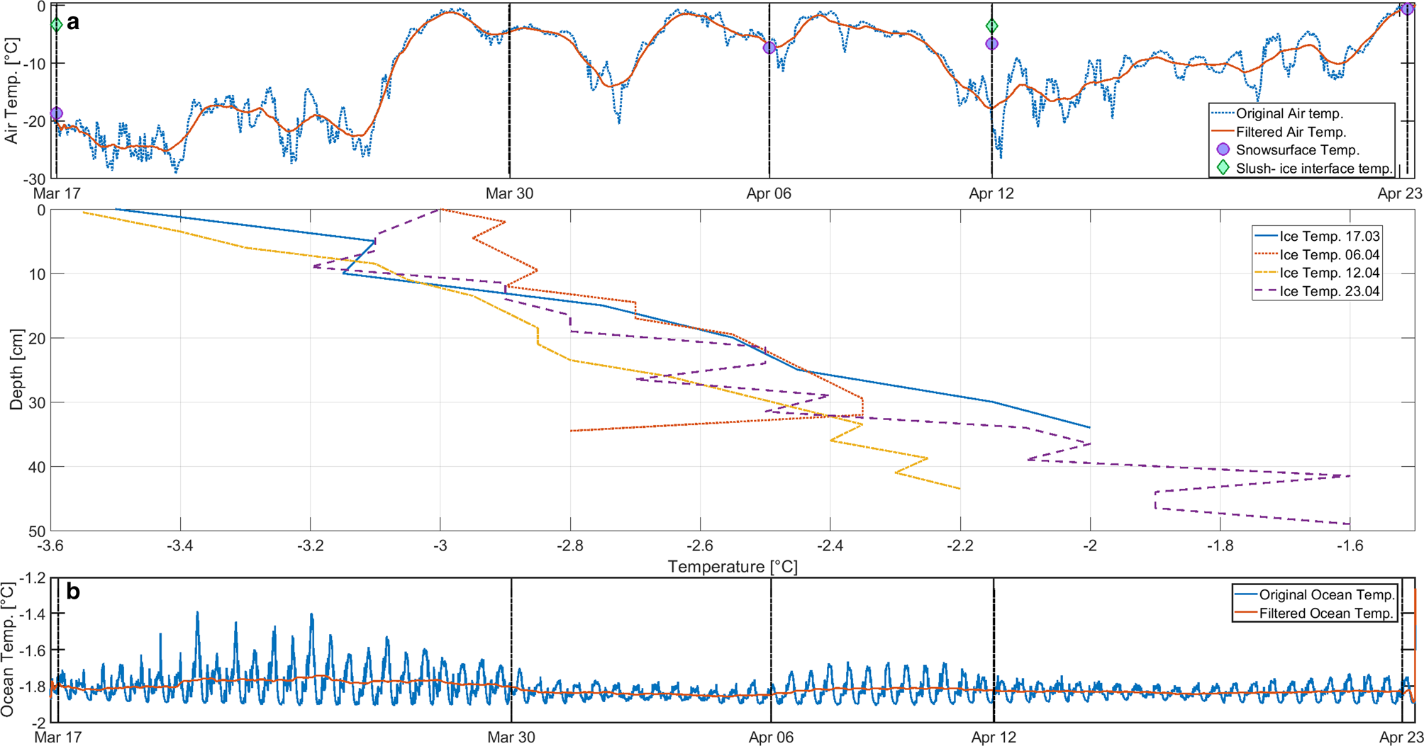
Green and blue circles in Figure 4b give the temperatures observed at the snow surface and at the snow slush/sea-ice interface, respectively (this interface was slushy in all cases). Figure 4b shows temperature profiles collected on each sampling day in °C over the ice thickness in cm. The profiles are averaged over two temperature profiles per day, where 0 cm refers to the sea-ice surface. On 30 March, the temperature sensor broke, so no temperature profile measurements are available for this day. We have, however, results from the installed logger that worked properly until this date. Temperatures are relatively constant and vary, at any level in the ice, by < 0.5 K over the sampling period. The low near bottom temperature on 12 April is very likely erroneous due to cooling of the sample during measurements.
In Figure 4c, ocean temperatures in °C are shown over the course of the field work. Ocean temperature was recorded at a depth of 1.2 m below the ice-air interface. There is a strong tidal signal present. Removing the latter using a simple running mean of 24 h, the mean ocean temperature was −1.8°C with a standard deviation of 0.1°C. The minimum of −1.9°C was reached on 26 March and the maximum ocean temperature was observed on 23 April with − 1.3°C.
Salinity
In Figure 5, salinity profiles are shown for each sampling day over the course of the field work. The salinity in psu is plotted over the ice thickness in cm. For each sampling day, the values shown were averaged from two cores. The two profiles in Figures 5a–e correspond to salinity based on conductivity of melted samples (blue), further called S con, and the salinity based on CT-scans (red), further referred to as S CT. S CT was calculated from porosity values at centrifuging temperature (mean −2.0°C) (Fig. 12a). S CT data are not available for 17 March, when samples were lost due to a cooling box failure. The vertical resolution of the measured S con as well as S CT was 2.5 cm. However, S CT are based on an approximately 10 times smaller volume. The salinity profiles based on the two methods are largely consistent with each other, while S CT are smaller than S con in the lower half of the ice. An exception to this is the very bottom on 30 March, yet here the cores had very different lengths. The vertical and time-averaged salinities, however, are consistent with each other with an average S con of 6.7 psu with a standard deviation of 2.1 psu, and S CT of 6.1 psu with a standard deviation of 4.2 psu. Note that all CT cores are slightly shorter because the weak skeletal layer was often destroyed during the cutting process.
Salinity profiles in psu and density proflies in kgm−3 plotted over the ice thickness in cm over the course of the fieldwork period from 17 March to 23 April 2016. 0 represents the sea-ice surface in contact with the atmosphere, numbers increase in depth towards the ocean. Grey dotted line represnets the boundary between columnar and granular ice. (a–e) Blue line represents conductivity measured salinity S con plotted over ice thickness and red shows the calculated salinity from porosity observed in CT-scans S CT at centrifuging temperature. (f–j) Blue line represents measurements from hydrostatic weighing ρ hydro and the red line presents calculated density from CT-Data ρ CT. ρ hydro and ρ CT at −2.7°C for 17 and 30 March and at −15°C for the sampling days in April.

Density
Density measurements are presented in Figures 5f–j. The plots show the density in kgm−3 over the measured ice thickness in cm. Hydrostatic density (ρ hydro) profiles are plotted in blue. ρ hydro was performed at −2.7°C for samples from 17 March and 30 March. ρ hydro measurements from the remaining field days were performed at −15°C. Density calculations based on evaluated air and brine porosity from CT-images (ρ CT) are presented in red. ρ CT was calculated on porosities at the same temperature as ρ hydro was conducted. On 17 March, samples for ρ CT were lost due to cooling problems, hence no density was calculated. The overall average ρ hydro from hydrostatic weighing is 900.5 kgm−3 with a standard deviation of 21.6 kgm−3. In comparison, ρ CT has a mean of 911.8 kgm−3 with a standard deviation of 9.8 kgm−3. ρ CT is on average 11.3 kgm−3 larger than ρ hydro, with a standard deviation of 4.4 kgm−3. The difference varies systematically over the thickness. Above a depth of 10 cm (with respect to the ice surface) the ρ CT is higher than ρ hydro, with differences of up to 20−80 kgm−3. This upper part of the ice includes the freeboard and snow ice.
Porosity
The porosity is given as volume fraction in $\percnt$ over the total analysed sample volume, shown in Figure 6 for both air (a–e) and brine porosity (f–j). Brine porosity measurements based on CT scans (ϕ′b) at centrifuging temperature (mean −2.0°C) in red are compared to brine porosity calculations based on salinity measurements ϕ brinecal at in situ temperature assuming thermal equilibrium given by Cox and Weeks in blue. For air porosity, CT-based values ϕ′air in red are compared to porosity estimates based on ρ hydro, ϕ aircal in blue. ϕ′bcon shows the connected part of ϕ′b presented in yellow. Again, all data points are based on averaging two cores, except for 17 March where CT samples were lost. It is seen that air porosities based on the two methods are largly consistent with each other, except in the upper 10–15 cm, where ϕ aircal values are considerably larger. At the ice surface, air porosity ϕ aircal based on hydrostatic density ρ hydro measurements reaches values from 3 to 9 vol.%. ϕ aircal shows a mean of 2.6 vol.% with a standard deviation of 2.0 vol.% and is by an average of 0.8 vol.% with a standard deviation of 0.6 vol.% larger than ϕ′air. ϕ′air has a mean value of 1.6 vol.% with a standard deviation of 0.6 vol.% Total ϕ′b shows a mean of 17.8 vol.% with a standard deviation of 11.4 vol.% at centrifuging temperature (mean − 2.0°C). Roughly two-third of ϕ′b are connected, with ϕ′bcon on average 12.2 vol.% and a standard deviation of 10.2 vol.%. ϕ′bcon correspond to the vertically connected brine porosity fraction of ϕ′bopen. ϕ′bopen shows a mean of 14.8 vol. $\percnt$
 with a standard deviation of 10.0 vol.%.
Total air ϕ′air, brine porosity ϕ′b and connected brine porosity ϕ′bcon in depth. Porosity in volume fraction $ \% $ over the total sample volume. Ice thickness measured in cm, 0 is ice surface. Number increase as ice thickness increase towards the ocean. Blue line presents theoretical air ϕ aircal and brine porosity ϕ brinecal according to Cox and Weeks at in situ temperature. Red line shows porosity data for brine ϕ′b and air ϕ′air at centrifuging temperature observed from CT-images. Yellow line presents connected brine porosity ϕ′bcon. Grey dotted line represnets the boundary between columnar and granular ice. (a) Air porosity from 17 March at −2.7°C, in (b) air porosity from 30 March is shown at −2.7°C, (c) presents air porosity from 06 April at −15°C, (d) shows air porosity from 12 April at −15 °C and (e) represents air porosity from 23 April at −15°C. (f) Brine porosity from 17 March, in (g) brine porosity from the 30 March is shown, (h) presents brine porosity from 06 April, (i) shows brine porosity from 12 April and (j) represents brine porosity from 23 April.

Pore scale characteristics
Pore number densities
We use two metrics for the number of pores in a sample, (i) the total number of open pores per area (OPN, for brine only) and (ii) the number of closed pores per volume (CPN for air and brine). The first is a measure of the number of connected brine channels; the second counts the air bubbles and brine inclusions. In Figure 7a, the profiles of OPN are based on counting the brine pores open to the lower side of the samples. Open pore numbers OPN fall between 5 and 50 per cm2. Except an increase in the bottom 5 cm of the ice, they do not show a pronounced depth dependence. The number decreases during the field work period. The number density of closed brine pores CPNbrine (Fig. 7b) falls mostly in the range 103 to 104 per cm3. The profiles show an increase both towards the top and the bottom. The number density of closed air pores CPNair (Fig. 7c) falls mostly in the range 200 to 1000 per cm3. The profiles also show an increase towards the top and the bottom. The profile from 23 April indicates vertical fluctuations with 5–10 cm thicker regimes of high and low pore numbers.
Number of pores per area in cm2, respectively by volume cm3 over ice thickness in cm. Grey dotted line represnets the boundary between columnar and granular ice. (a–d) Number of open pores per cm2 in z-minus direction. (e–h) Number of closed brine pores per cm3 in xyz-direction. (k–l) Number of closed air pores per cm3 in xyz-direction. The yellow line shows results for 30 March, red dashed line for 06 April, blue dashed dotted line for 12 April and the purple dotted line data for 23 April.

Pore size distributions
Pore and throat size distributions are presented in Figures 8–11a–d. The overall distribution for each sampling date from 30 March to 23 April is given for ϕ′air, ϕ′bclosed, ϕ′bopen and the throats. It is shown for a bin size of 25 μm as a volumetric distribution, rather than measuring the volume in each pore size class then counting their number. Again, all data points are based on an average of two cores per field day. The vertical dotted line indicates the separation into micro pores with pore sizes in the range 25 −700 μm and macro pores larger than 700 μm. The mode (maximum) and the median for the micro pores are presented as a red circle and a yellow square respectively. The median for macro pores is shown as a purple star. Analyses of the micro and macro pore fraction show that most of the pores appear as micro pores. The spatial resolution of the pore and throat size distribution is given in Figures 8–11e–h as the spatial resolution of the micro median and mode and the macro median in μm over the sea-ice thickness in cm. The median for micro pores is presented as a solid blue line, mode for micro air pores is shown as a dash-dotted green line, and the red solid line represents the median for macro pores.
Pore size distribution for air porosity. (a–d) Pore volume fraction for air in $\percnt$ plotted against the pore size in μm. Red circle presents mode, yellow square marks median of micro pores and the purple star represents the macro median. (e–h) Median and mode for air pore size distribution in μm plotted over ice thickness in cm. Grey dotted line represnets the boundary between columnar and granular ice.

Air pores
The air pore size distribution is presented in Figure 8 for the four sampling dates. The distribution shows the broadest spectrum of pore sizes on 30 March with pore sizes up to 2575 μm. The micro mode typically lay in the range of 200–225 μm. The micro median is also here slightly larger with typical values from 225 to 275 μm. No change in these characteristics is apparent over time. For the macro pores, the mode decreases from 1000 μm to 800 μm over time. This, however, is related to two samples from 30 March (at 3 and 25 cm depth) with some extremely large pores. The macro pores show a larger vertical variation with the biggest variety at the very beginning of the experiment. The smallest air pore medians are, for both the micro and macro pores, observed near the ice-ocean interface.
Closed brine pores
Pore size distribution of the closed brine fraction at −15°C shows pore sizes up to 875 μm (Fig. 9). Most pores are smaller than 700 μm, and just an insignificant part of the pores can be found in the spectrum of the macro pores. Therefore no differentiation between micro and macro pores for the closed brine fraction is made. A constant mode of 50 μm is found over all the sampling days, with the median varying between 75 and 100 μm. These values indicate the limitation in our spatial resolution (Nyquist limit of two times voxel size is 50 μm). For both the mode and the median, no significant evolution over time and temperature can be observed. The spatial distribution over median and mode for the brine closed volume fraction are typically found between 60 and 160 μm.
Pore size distribution for closed brine porosity at − 15°C. (a–d) Pore volume fraction for closed brine in $\percnt$ plotted against the pore size in μm. Red circle presents mode and yellow square marks median of micro pores. (e–h) Median and mode for closed brine at − 15°C pore size distribution in μm plotted over ice thickness in cm. Grey dotted line represnets the boundary between columnar and granular ice.

Open brine pores
Pore size distribution for the open brine volume fraction shows a spectrum up to 3125 μm (Fig. 10). The micro mode can be found between 200 and 300 μm and the micro median ranges from 275 −375 μm. The macro pore median varies from 1025 −1275 μm. The biggest macro pore median is found on 12 April in the top 4–10 cm. The smallest macro pore median can be found in the bottom most samples towards the ocean interface.
Pore size distribution for open brine porosity. (a–d) Pore volume fraction for open brine in $\percnt$ plotted against the pore size in μm. Red circle presents mode, yellow square marks median of micro pores and the purple star represents the macro median. (e–h) Median and mode for open brine pore size distribution in μm plotted over ice thickness in cm. Grey dotted line represnets the boundary between columnar and granular ice.

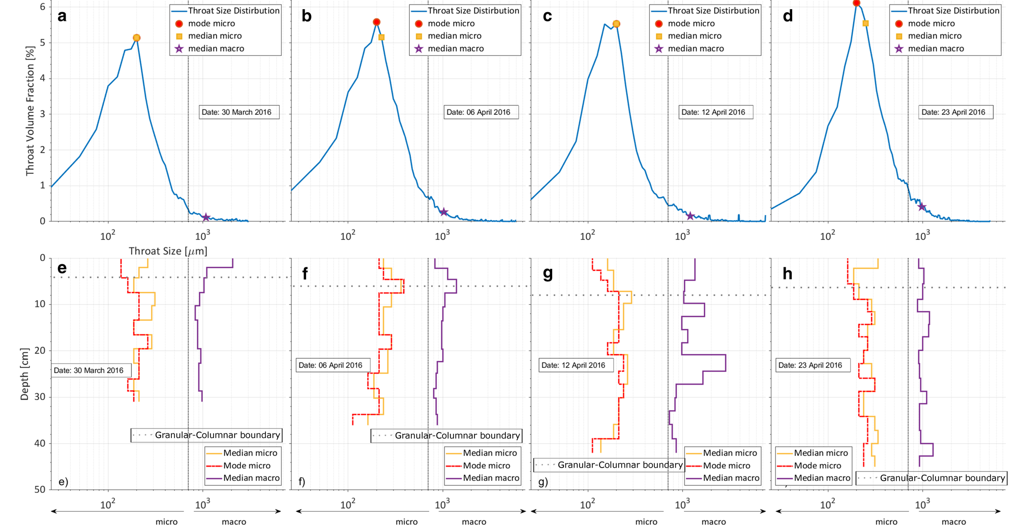
Throat size distribution
The throat size distribution (Fig. 11) stretches up to 7425 μm with constant micro modes and a value of 200 μm. The micro median varies from 275−375 μm, the minimum can be seen on 12 April and the maximum on 23 April. The macro pore median increases from 1075 μm on 30 March up to 1275 μm before it decreases again to the minimum macro median of 975 μm on 23 April. Spatial resolution of the micro median and mode varies typically from 125−375 μm. The spatial resolution of the macro median ranges from 725−2852 μm with the maximum found on 12 April.
Throat size distribution for open brine porosity. (a–d) Throat volume fraction for open brine in $\percnt$ plotted against the pore size in μm. Red circle presents mode, yellow square marks median of micro pores and the purple star represents the macro median. (e–h) Median and mode for throat size distribution in μm plotted over ice thickness in cm. Grey dotted line represnets the boundary between columnar and granular ice.
Discussion
The goal of our study has been to obtain 3-D microstructure information on natural sea ice that reflects its in situ stage as closly as possible. This is a challenge because on the one hand we have to minimise changes in sea-ice microstructure due to temperature, internal freezing and brine drainage, and on the other hand we need to ensure that samples are sufficiently stable during 3-D μCT acquisition of up to several hours. Moreover, the approach requires sufficient X-ray contrast to distinguish between ice and brine. To do so, we have applied a three-step procedure. First, we have transported and stored sea-ice samples at temperatures close to their in situ values in the field. Next, we have centrifuged these samples on the following day (also close to their in situ temperatures), which removes the highly mobile connected brine volume fractions. Finally, we have stored these samples at low temperatures until X-ray scanning. The latter approach is essential to obtain high-quality images for pore space analysis at high temperatures Maus (Reference Maus2020). Other approaches, like adding a contrast agent (Pringle and others, Reference Pringle, Miner, Eicken and Golden2009) or imaging samples at high enough brine concentration and low temperature (Obbard and others, Reference Obbard, Troderman and Baker2009), are not practical for warm natural sea ice. Overall, the procedures bear potential for a number of errors and biases, of which the following are considered most important:
(1) Transport and storage have been performed with mobile freezers with a nominal temperature accuracy of ± 0.5 K, which can be improved by calibration with other temperature sensors. However, we found that the response of the temperature control of the mobile freezers was less predictable for rapidly changing environmental conditions (from − 20°C in the field to 10−20°C in different labs and storage rooms).
(2) A similar problem as for the transport and storage was observed with the temperature stability in the centrifuge. Overall, this resulted in sample temperatures during processing that were 0.3–1.3 K lower than in situ values.
(3) The quality of salinity calculations based on CT observations depends on several factors related to the determination of the salinity in open and closed pores. For the open pores the assumption is made that all these pores were filled with brine with the same salinity as the centrifuged brine. This assumption may be wrong in the upper part of the ice including the freeboard and snow-ice, where pores may have drained. For the closed brine-filled pores, the quality depends on the spatial resolution and the question of how many pores have sizes below the latter and thus remain undetected. It also depends on proper choice of the segmentation threshold.
Despite these problems in obtaining CT images exactly at in situ conditions, the present study has not only collected a new dataset of 3-D microstructure and pore scale properties of young sea ice, but has also provided information about the change of these properties over the course of 3 1/2 weeks. In the following discussion, the focus will be on sea-ice bulk and pore space property changes over time and on its dependence on the brine porosity ϕ′b. The vertically averaged bulk properties and pore space characteristics for the sampling dates are summarised in Figures 12 and 13.
Overview over measured parameters: (a) average air temperature in °C for each sampling day, plotted in blue. Average ice temperature for each sampling day over ice depth plotted in red. (b) Average measured salinity S con for each sampling day over ice depth in psu plotted in blue. Mean salinity in psu calculated S CT for each sampling day at centrifuge temperature over ice depth, observed from brine porosity in CT-scans are shown in red. (c) Average hydro-static determined density ρ hydro in kg/m3 for each sampling day over ice depth plotted in blue. Calculated density ρ CT from CT-images plotted in red. (d) In blue theoretical air porosity ϕ aircal following Cox and weeks in vol. %, in red air porosity observed from CT-images ϕ′air, in yellow the observed brine porosity from CT-scans ϕ′b at centrifuge temperature, in purple the theoretical brine porosity ϕ′brinecal at in situ temperature following Cox and weeks, in dark green the open brine porosity ϕ′bopen at centrifuge temperature and in light green the connected brine porosity at centrifuge temperature ϕ′bcon for each sampling day over the ice depth is shown.

Overview over measured parameters: (a) average OPN in z-minus direction per cm2 for each sampling day, plotted in blue. Average CPNbrine in xyz-minus direction per cm3 for each sampling day plotted in red and the average CPNair per cm3 in yellow. (b) Mean pore size in μm for ϕ′bopen plotted for each day in blue, ϕ′bclosed in red, ϕ′air in yellow and the mean throat size in purple for each day at a temperature of −15 <. (c) Median pore size in μm for ϕ′bopen plotted for each day in blue, ϕ′bclosed in red, ϕ′air in yellow and the median throat size in purple for each day at −15 °C. (d) Macro pore fraction in $\percnt$ for ϕ′bopen plotted for each day in blue, ϕ′bclosed in red, ϕ′air in yellow and the macro throat size in purple for each day at −15°C.

Bulk properties
Temperature
Over the course of the field work, the temperature gradient was relatively weak. This made it feasible to transport and centrifuge the ice close to its in situ temperature with limited logistics. The comparison of the average ice temperature per day with the average centrifuge temperature (Fig. 12a) suggests that the centrifuge temperature, computed from the salinity of centrifuged brine, was systematically higher than the in situ ice temperature, with an average difference of 0.7°C. Larger temperature differences were observed in the uppermost and lowermost parts of the ice cores and are related to the above-mentioned imperfect temperature control. Since the difference was not constant (being 0.3 K on 30 March and 12 April compared to 1.2 K on 06 April and 23 April), this has to be taken into account in the interpretation of brine fraction observations and all associated parameters as well as pores size changes, and will be discussed below.
Salinity
Figure 12 summarises the evolution of average temperature and salinity during our field work. The vertically averaged salinity S con during our field work shows typical values in the range 5.9–7.4 psu, at the upper end of the range 3.5–6.5 ppt that Høyland (Reference Høyland2009) reported for sea ice of a similar age (3–4 months) from different locations in Van Mijenfjorden. The average salinity did not change significantly during the field work. The average S CT at temperature T CT shows a mean of 6.1 psu with a standard deviation of 4.2 psu and is on average 0.6 psu lower than S con (Fig. 12b) with a mean of 6.7 psu and a standard deviation of 2.1 psu. For the individual sampling dates, the differences range between 1.4 psu larger S con and 0.1 psu larger S CT. Natural variability between different cores, internal variability of samples and the fact that S con is based on ten times smaller sample volumes may all contribute to the differences. The comparison between vertical profiles of S con and S CT shows broad agreement, yet considerable scatter (Fig. 5).
An underestimation of salinity based on CT data can result from resolution limitations in the CT images, as objects smaller than two times the voxel size of 25 μm pixel cannot be resolved (Nyquist–Shannon theorem). Looking at the pore size distribution of closed brine pores (Figs 9a–d) we find that around 16% of the closed pores have diameters of 2 voxel (50 μm) and 13% are in the 1 voxel size class of 25 μm. Combining this with our finding that the detected closed pores contain about one-sixth of the salt (see discussion below), these correspond to fractions of 3 and 2% of total brine porosity (and salinity). To estimate the number of undetected pores one would need reference data at a higher resolution. Light and others (Reference Light, Maykut and Grenfell2003) observed numerous brine pockets with a size below the resolution of this study, and as small as 10 μm, which they classified according to their length (in 2-D optical images) and their aspect ratio. Brine inclusions with diameters <50 μm in our study would roughly correspond to the classes of brine pockets with lengths <100 μm in their Figure 8, containing roughly 3% of the total brine volume. Hence, this comparison would not indicate a considerable fraction of undetected pockets. However, there is general lack of data on small inclusions, and Light and others (Reference Light, Maykut and Grenfell2003) noted that they were only able to visually detect 2/3 of the conductivity-based brine volume. Maus and others (Reference Maus, Schneebeli and Wiegmann2021) also noted the difficulty of segmenting brine, because ice has a similar absorption as a mixed air-brine pixel, ending up with uncertainties of 1% for closed brine porosity. Related to total porosity of 10–20%, this would change the salinity by 5–10% or 0.3–0.7 psu. Hence, the difference of + 0.8 to − 0.5 psu between conductivity and CT-based salinity is within the error bounds expected from image analysis and a resolution limit of brine pore detection.
However, more critical is the systematic vertical distribution of the difference, with S CT larger than S con in the upper ice, and lower in the lower portion of the ice. For the lower portion, a possible source of error is loss of brine during sampling. Normally, one would expect that S CT based on the open pore space is not affected by the loss of brine during sampling. However, if slow brine loss is considered (leakage of brine during transport and prior to centrifuging), then the leaked brine would have a higher salinity than the centrifuged brine. Due to cutting samples to a smaller diameter prior to centrifuging, only the centrifuged brine salinity S cent is considered to compute S CT with Eqn (3), and this would lead to an underestimated S CT value. In a different study, one of the authors determined that, during similar storage and transport procedures, 28% of the total connected brine (leaked and centrifuged) leaked out prior to centrifugation Maus and others (Reference Maus, Schneebeli and Wiegmann2021). If this brine had two times the centrifuged brine porosity, this would increase the bulk salinity due to connected brine pores by 28%. Considering that another 25% of salt is contained in closed brine pores, the bulk salinity would be underestimated by 20%, or for our profiles by 1–2 psu. A vice versa argumentation holds for the upper part of the ice – the freeboard. Here, the ice has drained naturally, many connected pores are empty, yet are interpreted as connected brine pores in the CT-based analysis. Hence, here the estimates of S CT will overestimate the in situ salinity. Note that all these contributions could be quantified by accurate determination of the masses of leaked and centrifuged brine, which in our study by sampling and centrifuging samples of different diameters, was not done. However, the estimates indicate that differences between conductivity S con and CT-based salinity S CT of 3–4% as found near the bottom on 12 April cannot be explained by brine leakage alone. Here, the low salinity of the CT samples must be related to natural variability on a scale of a few centimeters.
Brine porosity
Salinity is a largely conservative property, while the brine porosity depends on temperature, and is thus different for the in situ and centrifuged-based calculations. Figure 6 shows that most centrifuge-based porosities are larger, simply because the centrifuge and storage temperatures were larger. We also see that the in situ porosities show a decrease towards the top, where the ice is colder, while the centrifuge and CT-based porosities often show an increase towards the ice surface. The reason for this is that the transport temperature for individual samples was often lower than the in situ temperature near the bottom, but larger than the surface in situ temperatures. The overall CT-based porosities cover the range of 2–40%, while the in situ values were in the range 5–18%, and most of this difference is temperature-related.
Density and air porosity
On average, the density based on hydrostatic weighing ρ hydro, is smaller than the CT-based density ρ CT, the mean difference being 11.3 kgm−3, see Figure 12c. ρ hydro, with a mean of 900.5 kgm−3, has a much higher standard deviation of 21.6 kgm−3, compared to ρ CT with an average of 911.8 kgm−3 and a standard deviation of 9.8 kgm−3. The difference between the density estimates is strongly dependent on the vertical position (Figs 5f–j). In the upper ice, including the freeboard and snow-ice, the CT-based densities are much larger, while in the rest of the ice, below 10–15 cm depth, the values are similar or the CT-based values are slightly lower. An exception to this, as for the salinity, is the bottom sample on 30 March, where an exceptionally high CT-based density is related to an exceptionally high salinity.
For the large difference between ρ hydro and ρ CT in the upper part of the ice cores, we have, as for the salinity, the following explanation. ρ CT is calculated on the air and brine porosity observed from centrifuged samples, where the entire open air space was assumed to be brine filled at in situ conditions. However, as the brine in the upper part of the ice including the freeboard and snow-ice has often drained, and thus the open air space is not brine-filled, the latter assumption overestimates the density. The correct value at the surface is thus the hydrostatic density ρ hydro. Below the freeboard, the values are much more consistent. Comparison of the density profiles without the uppermost 15 cm show a mean difference of 4.1 kgm−3 with a standard deviation of 7.7 kgm−3 where ρ hydro tends to be larger than the ρ CT. Temperatures during CT core storage and centrifuging were larger than in situ values in the upper ice, and lower near the ice bottom. This may result in lower ρ CT near the bottom and larger values close to the top. Nakawo and Sinha (Reference Nakawo and Sinha1981) describes decreasing density profiles and an increase in air porosity towards the top, as it is observed from ρ hydro profiles in Figures 5f–j and 6a–e.
Based on the same consideration, it follows that the CT-based air volume fraction ϕ′air is underestimated in the upper part of the ice including the freeboard and snow-ice (see Figs 6a–e). Averaging over the whole ice thickness gives a mean ϕ′air of 1.6% with a standard deviation of 0.6%. The mean ϕ aircal based on hydrostatic weighing is 2.6% with a standard deviation of 0.6%. The CT-based vertically averaged ϕ′air is thus on average 0.8% smaller than ϕ aircal. However, the CT-based air porosity ϕ′air can be expected to be valid for ice below the freeboard. Comparison of ϕ′air and ϕ aircal without the top 15 cm, gives larger CT-based air porosities, with a mean difference of 0.4% in comparison to ϕ aircal with a standard deviation of 0.5%. A look into the profiles indicates this difference may be related to natural variability, but also resolution and/or measurement errors may be relevant. Firstly, CT-based air porosities may be too small due to undetected air pores below our spatial resolution. A look into the air pore size distribution in Figure 8 indicates that this effect is likely negligible for our samples. Secondly, the density calibration during hydrostatic weighing is limited by the aerometer's uncertainty to obtain the density of paraffin (in our case 0.2%). Thirdly, one could suspect that hydrostatic weighing overestimates the air porosity, because it cannot distinguish between leaked brine and closed air pores. The latter seems not to be a problem in our study. As air porosity is a rarely measured property, there are not many observations for comparison. Lieb-Lappen and others (Reference Lieb-Lappen, Golden and Obbard2017) observed in a micro-CT study of non-centrifuged first year sea ice, that the air phase represents <1% in a volume of 7.5 mm3. Nakawo (Reference Nakawo1983) has obtained air porosity based on density measurements as well as the volume of released gas during melting of samples. He reports a range 0.3–1% air porosity below the freeboard, and values of up to 5% in the freeboard of 1 m thick first-year ice. Values Nakawo (Reference Nakawo1983) reports are slightly below our observed range. Pustogvar and Kulyakhtin (Reference Pustogvar and Kulyakhtin2016) reports air porosities based on hydrostatic weighing, with similar values to what we found in the upper part of the ice. Below the freeboard they observe a range from 0.1 to 2.7%, which is comparable to our measurements, yet with larger variation. Crabeck and others (Reference Crabeck, Galley, Delille, Else and Geilfus2016) observed, based on mass-volume density measurements, air volume fractions of 1–2% in the lowermost layer, in the middle part of the profiles air volume fractions of typically 1.5–4% and in the uppermost part 4–10%. However, these values were subject to large uncertainties, as the density was not obtained by the hydrostatic method. Crabeck and others (Reference Crabeck, Galley, Delille, Else and Geilfus2016) obtained much lower CT-based air porosities, often less then half the density-based values (their Figure 10), in all levels of the ice. This underestimation can be attributed to their spatial resolution (pixel size 97 μm, Nyquist criterion of 194 μm). Since we find most median air pore sizes between 225 and 275 μm, see Figure 8, this would imply that roughly half of the air pore volume would not have been detected at such a resolution. Obbard and others (Reference Obbard, Troderman and Baker2009) reported an air volume fraction of 1.96% for one sea-ice sample imaged with a resolution of 15 μm and comparable to samples below the freeboard of the present study.
Pore space characteristics
Open and connected brine porosity
The CT-based values allow to determine the aspects of the pore space which are not given by the in situ bulk properties as the open brine porosity ϕ′bopen, the closed brine porosity ϕ′bclosed and the vertically connected brine porosity ϕ′bcon. ϕ′bcon ranges, with a vertical average over the four sampling dates, between 6.2 and 19.4% (Fig. 12), corresponding to 48–80% of the total brine porosity ϕ′b. Individual values for ϕ′bcon in dependence on ϕ′b are plotted in Figure 14 and range from 0 to 35%. An almost linear increase in ϕ′bcon with the total brine porosity ϕ′b is observed. For a total brine porosity below 3% no vertical connection within the samples is found, e.g. near the bottom on 12 April, where the minimum CT-based salinities S CT also occur (Fig. 5). ϕ′bopen ranges with a vertical average between 9.7 and 21.6%. As the residual brine porosity ϕ′bclosed is related to ϕ′bopen by (ϕ′bclosed = 1 − ϕ′bopen) this corresponds to a relative closed brine pore fraction in the range of $11\% < \phi '_{{\rm b\ closed}}/\phi '_{\rm b} < 25$ %. This range is consistent with other centrifuge studies at high porosities and temperatures Maus and others (Reference Maus, Schneebeli and Wiegmann2021); Weissenberger and others (Reference Weissenberger, Dieckmann, Gradinger and Spindler1992). The individual values of open brine porosity ϕ′bopen are shown in Figure 14a dependent on the total porosity. A close to linear increase in open porosity with total brine porosity is apparent. Maus and others (Reference Maus, Schneebeli and Wiegmann2021) discusses ϕ′bopen and ϕ′bcon, and their dependency on ϕ′b for slightly younger ice, and describes the relationship by

where C is a constant and ϕ bcrit is a threshold porosity that was determined as ϕ bcrit ≃ 0.024 for young ice. The exponent β is related to the percolation theory. Maus and others (Reference Maus, Schneebeli and Wiegmann2021) determined β ≃ 0.83 for the open brine porosity ϕ′bopen and as β 2 ≃ 1.2 for the connected brine porosity ϕ′bcon, from data of columnar young ice in the porosity range of 1–20%. The relationships given by Maus and others (Reference Maus, Schneebeli and Wiegmann2021) are shown in Figures 14a and 14b as dashed magenta curves. In the present study, little data close to the percolation threshold were found, thus an assumption of ϕ bcrit ≃ 0.024 is made, and obtained comparable fits by application of a double-logarithmic regression. For ϕ′bopen, β ≃ 0.87 ± 0.07, while for ϕ′bcon, β ≃ 1.10 ± 0.17 is found. As discussed by Maus and others (Reference Maus, Schneebeli and Wiegmann2021), the open brine porosity exponent is consistent with the theoretical estimate β ≃ 0.82 for directed percolation. Data presented are from ice cores taken over the period of one month, containing both columnar and granular ice, with a brine porosity ϕ′b range from 1 to 55%, while Maus and others (Reference Maus, Schneebeli and Wiegmann2021) studied columnar ice sampled over one week, at lower temperatures and a brine porosity range from 1 to 20%. Data presented in our study start to deviate from the relationship given by Maus and others (Reference Maus, Schneebeli and Wiegmann2021) at porosities above 10–15%. Though there is overall good agreement between these studies, more detailed analysis should take differences in high and low porosity regimes and the difference between granular and columnar ice into account. The connected porosity ϕ′bcon increases with a higher exponent β ≃ 1.10 ± 0.17 than the open porosity, in close agreement with the exponent of β ≃ 1.2 ± 0.1 by Maus and others (Reference Maus, Schneebeli and Wiegmann2021). Based on our least square fits, ϕ′bopen and ϕ′bcon match at a total brine porosity of 45%, where they both are predicted as 36.8%. Due to the uncertainties in the fits, we do not attribute a physical meaning to this value, but rather interpret it as a validity limit, as the connected porosity cannot be larger than the open porosity.
(a) Open brine porosity ϕ′bopen and (b) connected brine porosity ϕ′bcon plotted against total brine volume fraction ϕ′b for each day. 30 March is represented in yellow, 06 April is shown in red, 12 April is plotted in blue and 23 April is represented in purple. Grey line representing the percolation threshold. Yellow line least square fit for ϕ′bopen and ϕ′bcon against ϕ′b. Purple line fit following Maus and others (Reference Maus, Schneebeli and Wiegmann2021) for total brine porosity $\leq 2\percnt$ .
.

Figures 14a and 14b also indicate a difference between sampling dates, as seen when focussing on the colour code. For brine porosities above 20%, ϕ′bopen and ϕ′bcon values from 23 April at the same total brine porosity ϕ′b, are higher than values from 06 April and 12 April. Hence, there appears to be a relative increase in the open porosity ϕ′bopen and a corresponding decrease in the closed porosity ϕ′bclosed. This increase is only observed for the sampling date 23 April, but not between 30 March and 12 April, and thus it is not happening constantly over time. As shown in Figure 16 and discussed below, 23 April is also exceptional in terms of pore numbers. The evolution is thus consistent with a transition from a higher number of smaller and disconnected pores to a smaller number of connected pores with larger diameter and length.
Pore number density
Pore numbers shown in Figure 7 are further investigated depending on the total brine porosity in Figure 15. We recall that open brine pore numbers are given per cross-sectional area, while closed air and brine pore numbers are given per volume. The vertical average for the sampling dates is given in Figure 13, with a minimum for the OPN on 23 April with 14 pores per cm2 and a maximum of 32 pores per cm2 on 30 March. As seen in Figure 7a, the overall variation in OPN is between 5 and 80 per cm2. A correlation between the measurements taken for the OPN and the brine porosity suggests a slight but significant decrease in OPN with increasing brine porosity (Fig. 15a). Most of this decrease is related to the much lower OPN on 23 April, compared to the other sampling dates.
(a) Open pore number per cm2 in z-direction plotted against total volume brine fraction ϕ′b for each day. (b) Closed brine pore number per cm3 shown against the total brine volume fraction ϕ′b. (c) Closed air pore number per cm3 in xyz-direction plotted against total brine volume fraction ϕ′b for each day. Yellow represents data from 30 March, red shows data from 06 April, in blue measurements from 12 April and in purple data points from 23 April.

For the CPNbrine closed brine pore numbers, no significant trend dependent on the brine porosity ϕ′b is observed (Fig. 15b). Most data fall in the range 1–10 pores per mm3, with an average of 3.8 pores per mm3 and a large standard deviation of 5.2 pores per mm3. An exception to this are the significantly lower pore numbers from 23 April (on average 1.5 pores per mm3). This change is consistent with the decrease in closed brine porosity ϕ′bclosed described above, and likely related to merging, coarsening and opening of pores. The results can be compared to reported pore statistics from other studies. Light and others (Reference Light, Maykut and Grenfell2003) reported an average number density of 24 pores per mm3 for thicker first-year ice. This higher number is likely related to the higher resolution in that study (down to 10 μm compared to our 25 μm voxel size). Our results are comparable to the brine pocket numbers reported by Perovich and Gow (Reference Perovich and Gow1996) for young and first-year ice, being in the range 1–6.9 pores per mm3. Perovich and Gow (Reference Perovich and Gow1996) obtained these numbers from optical analysis of 2-D thin sections with a similar pixel size (0.03 mm) as in our study. It is noteworthy that Perovich and Gow (Reference Perovich and Gow1996) found a complex change in number density of brine pockets with porosity: at high porosities they observed a decrease in the brine pore number densities with porosity, attributed to coalescence of pores. However, for the porosity range from 3 to 20%, they observed an increase which they attributed to the increase in pore sizes above their detectability threshold. Our data show too high variability to indicate such behaviour. However, we observe, for porosities above 15%, a continuous decrease in close brine pore numbers over time from 06 April to 23 April (seen in the colour coding in Fig. 15b).
The number densities of closed air pores, CPNair, are mostly found in the range 0.1–1 pores per mm3, an order of magnitude of 10 smaller than for the closed brine pores CPNbrine (Fig. 15c), and with an average of 0.32 pores per mm3. Also here, the decreasing trend with porosity is mostly related to the significantly lower pore numbers from 23 April (on average 1.5 pores per mm3). This change is consistent with the decrease in closed brine porosity described above, and likely related to merging, coarsening and opening of pores. The results can be compared to reported pore statistics from other studies. Also here the average number density of 1.2 per mm3 reported by Light and others (Reference Light, Maykut and Grenfell2003) is significantly larger, which again can be attributed to the higher resolution in the latter study. Light and others (Reference Light, Maykut and Grenfell2003) also reported earlier observations of air bubble numbers in young ice that were an order of magnitude lower than ours (0.03 pores per mm3). Our study does not resolve the smallest air pores, but provides two other interesting findings. First, an observed decrease in air pore numbers at high porosities, that is likely attributable to the reopening and coalescence of brine pores. Second, as shown in Figures 7i–l, air pore numbers are larger near the bottom and surface of the ice, than in the middle.
Pore and throat size
Both the median (Fig. 16) as well as the macro pore fraction (Fig. 17) for the open pores and throat sizes show a significant increase with the total brine porosity ϕ′b. Comparison of pore- and throat sizes shows that pore sizes are by a factor of roughly 1.5 larger (Fig. 16a). An increase in pore and throat sizes is expected during warming when internal melting increases the brine porosity and thus widens the pores. If no pores coalesce or split, a diameter D ~ ϕ′b 1/2 for brine tubes and D ~ ϕ′b 1/3 for spherical brine inclusions are expected. However, we observe smaller exponents of 0.24 for the median pore and 0.22 for throat diameters. This indicates a different pore widening process than for simple cylindrical pores. In general, this observation is not inconsistent for widening processes in sea ice. For example, if pores develop from original vertical brine layers, they tend to be anisotropic in a horizontal cross section Perovich and Gow (Reference Perovich and Gow1996), if those pores primarily expand in longitudinal direction by dissolution of ice, the shorter direction of the pore (measured with the sphere fitting algorithm in Geodict) will be less affected by porosity changes.
(a) Median pore size in μm for ϕ′bopen plotted with stars, throatsize represented as squares are plotted against the total brine volume ϕ′b in $\percnt$ for each day. (b) Median pore size in μm for ϕ′bclosed and (c) median pore size for ϕ′air are plotted against ϕ′b in $\percnt$
 for each day. 30 March is represented in yellow, 06 April is shown in red, 12 April is plotted in blue and 23 April is represented in purple.

(a) Macro pore size fraction in $\percnt$ for ϕ′bopen (b) throatsize and (c) ϕ′air the throatsize represented as diamonds are plotted against the total brine volume ϕ′b in $\percnt$
 for each day. 30 March is represented in yellow, 06 April is shown in red, 12 April is plotted in blue and 23 April is represented in purple.

A similar weak dependency of pore diameters on porosity has been observed by Perovich and Gow (Reference Perovich and Gow1996) for a warming sequence. For young ice that was cooled than warmed prior to X-ray imaging, and with most data in the porosity regime between 3 and 15%, Maus and others (Reference Maus, Schneebeli and Wiegmann2021) obtained exponents of 0.34 for pore and 0.46 for throat sizes. Hence, the details of pore size redistribution during warming and cooling appear to be complex, and should be studied in more detail. The median throat and pore sizes obtained in the present study exceed those obtained by Maus and others (Reference Maus, Schneebeli and Wiegmann2021) by roughly a factor of 1.5. This may be attributed to the greater thickness and age of the present ice (2 months compared to 3 weeks in the latter study) and the higher number of wider brine channels in the older ice. It is further noted that neither for throat nor pore sizes exceptional values are observed for 23 April, quite in contrary to the pore numbers.
The pore sizes for closed brine PS bclosed show an insignificant decrease in pore size with total brine porosity. This is not surprising, as the closed brine pores were all imaged at the same temperature of − 15 °C, and were unaffected by the centrifuging technique and temperature. We interpret the slight decrease towards 06 and 23 April, for the warmer cores and higher porosity, with a likely merge between the larger brine pores and the open porosity, leaving pores with smaller diameters back.
Also for the closed air pores PS air no significant correlation with the brine porosity was found, again not surprising as the samples were all scanned at the same temperature and air pores should not be affected by centrifuging. Most air pores median diameters fall between 200 and 450 μm. The air pore population from 23 April does not appear as exceptional as for other properties of the pore space.
Analysis of the throat sizes showed that between 0.3 and 2.5 vol. have a diameter above 2 mm and increases from 30 March (0.3 vol.) to 06 April (2.5 vol.) before it decreases towards 12 April (2.4 vol.) and increases again towards 23 April (1.3 vol.). Throats above 2 mm are just presented in the upper 7.5 cm in the beginning of the experiment, at the end of the experiment they could be found from the bottom to the top of the ice core 11.
Conclusion
We have observed macroscopic and microscopic properties of young Arctic sea ice over the course of 1 month, prior to the onset of melting. Microscopic properties have been derived from the combination of two non-destructive techniques (i) centrifuging of brine for separation of the connected and disconnected pore space and (ii) 3-D micro-CT imaging followed by analysis of the pore size characteristics. Our main findings are
(1) Density and air porosity determinations based on hydrostatic weighing and CT images show good consistency within the range measurement accuracy (≈ 0.2 %) and natural variability (≈ 0.5 %).
(2) CT-based salinity determinations are subject to larger than standard uncertainties. Since, we reached the limitation of spatial resolution to resolve brine pores, while the strength is to distinguish different porosity metrics and to give a better understanding of where the salt is located (open, closed, vertically connected).
(3) The variation of different pore categories (open and closed brine pores, closed air pores) with vertical position in the ice is remarkably small – most variability is related to changes in the brine porosity.
(4) Most bulk properties (salinity, density) and pore space properties (pore sizes, proportion of secondary ‘macro’ pores) remained constant, while we observe significant changes in pore numbers (decreasing over time) and pore connectivity (increasing over time).
(5) We obtain confident relationships between the open (centrifuged) porosity ϕ′bopen, connected ϕ′bcon and total porosity ϕ′b of young sea ice.
(6) We further find that results are consistent with a connected brine porosity threshold of 2–3% as recently proposed by Maus and others (Reference Maus, Schneebeli and Wiegmann2021).
The agreement between our density and air porosity estimates ϕ′air and ϕ CT based on hydrostatic weighing and CT imaging below the freeboard is encouraging, as these properties have so far been mostly observed with high uncertainties. The difference in the upper part of the ice cores is related to our method centrifuging and imaging method, and would not be a problem for non-centrifuged samples. Here, future studies focussing on density only will be useful. The present approach, however, has provided important information about the morphology of the drained low-density surface regime, and the fractions of connected and disconnected air pores and will be useful to better understand the surface drainage and evolution of low-density layer.
The present study has provided pore space and pore size information with a spatial resolution (25 μm pixel/voxel size) two to four times better than in earlier work obtaining similar statistics on brine and air inclusions at relatively high temperature Eicken and others (Reference Eicken, Bock, Wittig, Miller and Poertner2000), Crabeck and others (Reference Crabeck, Galley, Delille, Else and Geilfus2016). To obtain pore sizes and connectivity metrics in this high temperature regime, centrifuging the samples is essential, as the absorption contrast between brine and ice would be too low to obtain high-quality 3-D images, with drainage during imaging being an additional problem. Imaging at a temperature as low as − 15°C Obbard and others (Reference Obbard, Troderman and Baker2009), Lieb-Lappen and others (Reference Lieb-Lappen, Golden and Obbard2017) would give sufficient contrast but cannot be used to derive the pore space connectivity metrics outlined here. Lieb-Lappen and others (Reference Lieb-Lappen, Kumar, Pauls and Obbard2018) performed network analysis on CT-images on sea ice with an in situ temperature as high as −7°C, yet they found differences between the CT-derived and salinity-derived brine volumes that increased with temperature, exceeding a factor of two. Due to such uncertainties, concise observations and modelling of pore size, number and connectivity (e.g. Figs 14 and 15) remain challenging tasks. An important issue for future studies is the scale-dependence of properties (e.g. connectivity, permeability, percolation threshold), that should be addressed by scanning larger samples with a larger FOV.
Acknowledgements
We gratefully acknowledge Aleksey Marchenko for hosting us at the Arctic Technology Department at The University Center in Svalbard (UNIS), Alkesey Shestov and UNIS Logistics for assistance and expertise regarding field and laboratory work, as well as Ole Tore Buset and Leander Michels for guidance and help during CT measurements at the Norwegian University of Science and Technology (NTNU). A big thanks to the field assistants Astrid Strunk, Eef van Dongen and Sarah Elise Sapper. Special thanks to Math2Market, GeoDict for providing the imaging analysis software. This work was supported by the Research Council of Norway PETROMAKS2 program, project number 243812 (MOSIDEO) and the Arctic Field Grant (AFG).
Appendix A
Table of variables
- β
exponent related to the percolation theory
- c
gives the phase relation between brine and solid salt
- C
constant
- CPN
number of closed pores per volume
- F SS
Factor to calculate the solid salt fraction from brine vol.
- f(T, T CT)
factor to convert brine fraction from T CT to T
- M air
mass in air
- M par
mass in paraffin
- OPN
total number of open pores per area
- ϕ air
air porosity
- ϕ′air
air porosity (CT-image derived in situ porosity)
- ϕ aircal
calculated air porosity based on hydrostatic density
- ϕ airopenz+
open air porosity to upper sample surface (CT)
- ϕ airopenz−
open air porosity to lower sample surface (CT)
- ϕ airopenz+−
open air porosity to lower and upper sample surface (CT)
- $\phi ^{CT}_{{\rm air}}$
air porosity (CT)
- $\phi ^{CT}_{{\rm airclosed}}$
closed air porosity (CT)
- $\phi ^{CT}_{{\rm aircon}}$
vertically connected air porosity (CT)
- $\phi ^{CT}_{{\rm airopen}}$
open air porosity (CT)
- ϕ b
brine porosity
- ϕ bclosed
closed brine porosity
- ϕ bcon
vertically connected brine porosity
- ϕ bcrit
threshold porosity
- ϕ bopen
open brine porosity
- ϕ′b
brine porosity (CT derived in situ porosity)
- ϕ′bclosed
closed brine porosity (CT derived in situ porosity)
- ϕ′bcon
connected brine porosity (CT derived in situ porosity)
- ϕ′bopen
open brine porosity (CT derived in situ porosity)
- ϕ brinecal
calculated brine porosity based on conductivity
- $\phi ^{{\rm CT}}_{{\rm brine}}$
brine porosity and solid salt (CT)
- ϕ con
connected porosity
- ϕ z+
open porosity to the upper sample surface
- ϕ z−
open porosity to the lower sample surface
- ϕ z+−
open porosity to the upper and lower sample surface
- ρ
sea-ice bulk density
- ρ air
air density
- ρ b
brine density
- ρ CT
bulk density from CT parameters at − 15°C
- ρ hydro
bulk density based on hydrostatic measurements
- ρ ice
ice density
- ρ par
paraffin density
- ρ ss
solid salt density
- S b
brine salinity
- S bdrip
dripped brine salinity
- S bcent
centrifuged brine salinity
- S cent
bulk salinity after centrifuging based on conductivity
- S con
bulk salinity based on conductivity
- S CT
bulk salinity based on CT
- S ice
sea-ice bulk salinity
- S rest
bulk salinity of cut-off
- T cent
centrifuge temperature
- T CT
CT temperature
- T
in situ Temperature


Appendix B
Illustration of granolometry and porosimetry
(a) Shows a structure with the solid material in white and the pore space in black. (b) Granulometry: shows the same structure with coloured pore volume, where the red volume describes the pore diameters around 40 μm and larger, green areas represent diameters around 20 μm and the blue-coloured area below 15 μm. (c) Porosimetry: structure shown in (a) gets penetrated with a non-wetting fluid, indicated by the red arrows. Pores found by porosimetry must be connected to the non-wetting phase. (after Linden and others, Reference Linden, Cheng and Wiegmann2018).

Appendix C
Illustration of vertical CT- reconstruction: Core 2-2 from 30 March
Vertical CT-reconstructions, showing ice in red, brine in green and air in white. Elongated, vertical oriented air inclusions (centrifuged brine) from sample 2-2-9 and downwards indicate granular sea ice. Sample 2-2-10 and 2-2-9 show a random pattern of air inclusions and are therefore interpreted as granular sea ice.


 Open access