


1. Introduction
Glaciers contribute significantly to sea level rise, with global glacier volume projected to decline by roughly 44% by 2100, equivalent to 19 cm of mean sea level rise 9-28 cm 90% confidence range; Fox-Kemper and others (Reference Fox-Kemper and Masson-Delmotte2021). Although smaller in magnitude than the long-term contribution from ice sheets, glacier retreat plays a crucial role over the shorter time horizons most relevant to climate mitigation and adaptation (Glavovic and others, Reference Glavovic, Dawson, Chow, Garschagen, Singh, Thomas and Roberts2021). Glacier mass loss also drives acute local hazards, including slope failures, glacier collapses and outburst floods (Carrivick and Tweed, Reference Carrivick and Tweed2016; Kääb and others, Reference Kääb2018; Shugar and others, Reference Shugar2021; Svennevig and others, Reference Svennevig2024).
Among glaciers, those that terminate in water—whether in the ocean (tidewater glaciers) or in proglacial lakes—stand out for their dynamism. For brevity, we refer to these collectively as water-terminating glaciers. Tidewater glaciers can undergo rapid cycles of advance and retreat (Meier and Post, Reference Meier and Post1987; O’Neel and others, Reference O’Neel, Pfeffer, Krimmel and Meier2005), while lake-terminating glaciers experience substantial subaqueous melt (Zhang and others, Reference Zhang2023). Much research has focused on process-level dynamics: calving laws (Vieli and others, Reference Vieli, Funk and Blatter2001; Nick and others, Reference Nick, van der Veen, Vieli and Benn2010; Sergienko, Reference Sergienko2022), mélange buttressing (Amundson and others, Reference Amundson, Fahnestock, Truffer, Brown, Lüthi and Motyka2010) and submarine melt (Sutherland and others, Reference Sutherland2019; Gräff and others, Reference Gräff2025). These studies have illuminated key mechanisms but leave open the broader question of how such processes shape the mean state of glaciers worldwide. Furthermore, most global-scale glacier models do not explicitly represent ice–ocean interactions, focusing instead on surface mass balance and simplified flow dynamics (Marzeion and others, Reference Marzeion2020). This omission limits their ability to capture the distinct geometry and volume of water-terminating glaciers.
Here, we ask a simple but revealing question: ‘for otherwise similar glaciers, are water-terminating glaciers on average thicker than their land-terminating counterparts?’ This perspective highlights the role of the ice front as a boundary condition on glacier flow (van der Veen, Reference van der Veen1996), where processes acting over small spatial and temporal scales collectively determine the large-scale equilibrium state. Calving dynamics, frontal melting, mélange buttressing and subaqueous melt each influence terminus mass and force balance, but their effects propagate far upstream through the force balance of the glacier. Theoretical studies have shown how calving laws can alter grounding line stability and the overall mass balance of marine-terminating glaciers (e.g., Schoof and others, Reference Schoof, Davis and Popa2017), underscoring the principle that localized physics at the terminus can reshape glacier-wide geometry. Our analysis captures this integrated outcome in the form of a shifted mean state: water-terminating glaciers tend to occupy a larger equilibrium geometry than their land-terminating counterparts, consistent with the additional support provided by water pressure at the ice front (Bassis and Walker, Reference Bassis and Walker2012).
By quantifying how this difference in mean state contributes to global ice volume, our data-driven approach complements process-based studies. We undertake a comprehensive uncertainty analysis (Section 3.4). The novelty of our approach is that we specifically exclude any water-terminating or ice shelf-supported glaciers in our training data. In this way, we derive a simple machine learning model that estimates glacier thicknesses in the absence of any glacier–ocean or glacier–lake interactions.
2. Data
This project uses two different datasets. The first dataset we use is the GlaThiDa database version 3.1.0 (Welty and others, Reference Welty2020). From this dataset, we extract the labels (dependent variables) for our analysis, specifically, glacier thickness and thickness uncertainty. GlaThiDa contains three separate datasets that describe different scales of measurement. We use only the ‘T’ dataset that contains glacier-averaged thicknesses, i.e., each data point represents the average thickness over an entire glacier. There are n = 500 unique glaciers in this dataset.
The second dataset we use is the Randolph Glacier Inventory, Version 6 (Arendt and others, Reference Arendt2017). From this dataset, we extract the features (independent variables) for our analysis. This feature vector has a dimensionality of six, and consists of glacier centroid latitude, centroid longitude, area, slope, elevation and maximum length. Later, we will also use the terminus type feature from the RGI dataset, although this information is not incorporated into our regression analysis. Unlike the GlaThiDa dataset, the RGI dataset is globally complete (n = 216501).
3. Methods
The main goal of our approach is to carry out a regression analysis that estimates the average thickness of individual glaciers given a set of glacier-scale features (maximum length, average slope, etc.). We accomplish this regression using a shallow neural network (SNN; see Figure 1 and Methods). We first train the SNN on the small number of glaciers for which we have in situ thickness information, and we then apply the model to the globally-complete RGI database. In this section, we describe in detail the workflow required to achieve this goal.
Our simple machine learning architecture features eleven inputs, normalization, two dense layers and a dropout layer.

3.1. Dataset coregistration
To combine glacier thickness observations from GlaThiDa with glacier outlines and attributes from the RGI, we must coregistered the two datasets so that each thickness measurement is paired with the correct glacier in the global inventory. Glaciers between the GlaThiDa and RGI catalogs are coregistered by finding the RGI glacier that is spatially closest to each GlaThiDa glacier. Although simple in principle, several complications occur in practice:
(1) Variable resolution of centroid coordinates in GlaThiDa sometimes introduces an ambiguity where several RGI glaciers may have numerical identical distances from a given GlaThiDa glacier or where one RGI glacier may have a numerically identical distance to several GlaThiDa glaciers. These cases are resolved by dropping the corresponding GlaThiDa glacier.
(2) Since years or decades may have passed between the epoch of the GlaThiDa and RGI measurements, there may not exist a well-defined match between the two catalogs. After matching by centroid location (as described above) a percent difference in size between entries in RGI and GlaThiDa is calculated as
(1) \begin{equation}
\Delta A_i = \frac{A_{k(i)}^\text{RGI} - A_i^\text{GlaThiDa}} {A_i^\text{GlaThiDa}}.
\end{equation}
\begin{equation}
\Delta A_i = \frac{A_{k(i)}^\text{RGI} - A_i^\text{GlaThiDa}} {A_i^\text{GlaThiDa}}.
\end{equation}This equation introduces the notation where indices
$i$ and
$k$ to refer to glaciers in the GlaThiDa and RGI catalogs, respectively. Coregistration involves determining the mapping between the two indices, i.e.,
$k(i)$.Equation 1 expresses the percent difference that represents changes in glacier surface area since thickness surveys were carried out and estimates the reliability of the available thickness data.
$\Delta A_i$ can also be compared to a threshold of uncertainty to dismiss any glaciers that may have unreliable labeled thickness for their measured size.(3) A small number of coregistered glaciers are found to occur over an unrealistically large distance. To quantify this effect, the ratio
$D = \frac{\Delta x}{r}$ is employed to compare the geometric glacier radius
$r = \sqrt{\frac{A^{\text{RGI} }}{\pi } }$, to the distance between catalogued glacier centroids,
$\Delta x$. Threshold
$T$ is then introduced to exclude erroneous coregistrations. Four thresholds are tested (
$T = 999, 0.75, 0.5, 0.25$) to find the ideal balance between sample size and reliability for training. These thresholds result in 400, 273, 202 and 105 labels, respectively. We discuss threshold selection below, after describing our shallow neural network (SNN) approach


3.2. Shallow neural networks (SNNs)
We carry out our regression analysis using a Shallow Neural Network (SNN; Figure 1). Our model is a two-hidden-layer multilayer perceptron (MLP) with ReLU activations, and a dropout rate of 0.1 between the hidden layers for regularization. Inputs are standardized with a Keras preprocessing. Normalization layer (used as the first layer). This layer is fitted on the training features only and performs per-feature z-score normalization (mean 0, unit variance). We train with early stopping on the validation loss, using a patience of 10 epochs and a minimum improvement of 0.001, restoring the best weights. Training runs up to 500 epochs but halts when the validation loss plateaus under these criteria, with these criteria being chosen to avoid overfitting.
With the goal of simplifying the parameters of the model, shallow neural networks (SNNs) with two layers of neurons are utilized. The network architecture consists of 6 neurons in the first layer and 2 neurons in the second layer surrounding a 10% dropout normalization layer to help prevent over-fitting (Srivastava and others, Reference Srivastava, Hinton, Krizhevsky, Sutskever and Salakhutdinov2014). We tested a wide range of architectures by varying the number of neurons in each of the two hidden layers; however, we found that this had minimal impact on our results and we do not further investigate this aspect of our model here. Learning rate and validation split (for early stopping) are held fixed at 0.01 and 0.2, respectively. Model residuals for the  $i^{\text{th}}$ GlaThiDa glacier are calculated as
 \begin{equation}
r_i = \hat{h}_i - h_i,
\end{equation}
\begin{equation}
r_i = \hat{h}_i - h_i,
\end{equation}and fractional residual
 \begin{equation}
R_i = \frac{\hat{h}_i - h_i}{h_i},
\end{equation}
\begin{equation}
R_i = \frac{\hat{h}_i - h_i}{h_i},
\end{equation}where  $h_i$ is the observed (GlaThiDa-reported) glacier thickness, and $\hat{h}_i$ is the corresponding estimated thickness. Model weights are calculated by minimizing mean absolute error (MAE), $\sum_{i=1}^{N_{\text{GlaThida}}} |r_i|/N_{\text{GlaThida}}, $ and mean squared error (MSE) $ \sum_{i=1}^{N_{\text{GlaThida}}} r_i ^2/N_{\text{GlaThida}},$ where $N_{\text{GlaThida}}$ is the number of glaciers in the GlaThiDa catalog. MAE describes how the model performs in estimating the average glacier, while MSE is more sensitive to larger errors which allows for discrimination against outliers.
3.3. Coregistration threshold selection
Although a strict coregistration threshold results matching glacier measurements more accurately, it also trades off against regression quality because fewer points are used. We quantify this tradeoff by examining model residuals (Equation 3) as a function of the threshold  $T$ (Figure S3). $T = 999$ represents all data regardless of area or location mismatch. This model does not perform well and estimates appear to hover around a mean value. $T = 0.25$ has very poor performance suggesting insufficient data for training. $T = 0.50$ and $T = 0.75$ estimates show improved performance. $T = 0.75$ is selected as the best fit to the data for further analysis.
3.4. Glacier volume and volume uncertainty calculation
For each of the  $n = 216501$ glaciers in the RGI catalog indexed by $k$, glacier volume is calculated as the product $\hat{V}_k = \hat{H}_k \hat{A}_k$ (no summation on the index $k$) of the estimated thickness $\hat H_k$ and area $\hat A_k$. We begin by analyzing the area $\hat A_k$ and thickness $\hat H_k$ terms separately, in Sections 3.4.1 and 3.4.2, before combining them to analyze volume in Section 3.4.3.
3.4.1. Glacier area and area uncertainty
The estimated area  $\hat A_k$ consists of the RGI-reported area $A_k$, which is modeled as a normal distribution,
 \begin{equation}
\hat A_k \sim \mathcal{N}\left[A_k,\text{Var}\left(A_k\right)\right].
\end{equation}
\begin{equation}
\hat A_k \sim \mathcal{N}\left[A_k,\text{Var}\left(A_k\right)\right].
\end{equation}Uncertainties due to mapping errors are quantified following the result of Pfeffer and others (Reference Pfeffer2014), who estimated area uncertainty with a simple model of fitting a curve to fractional uncertainties between multiple data sources for RGI. Their approximation yields the relationship
 \begin{equation}
\text{Var}\left(A_k\right) \approx c_1\alpha \left({A}_k^{p_1}\right)^2,
\end{equation}
\begin{equation}
\text{Var}\left(A_k\right) \approx c_1\alpha \left({A}_k^{p_1}\right)^2,
\end{equation}where  ${A}_k$ is the reported glacier surface area, $\alpha = 0.039$ is the estimated fractional error of a 1 km $^2$ glacier and $p_1 = 0.70$ and $c_1 = 3$ are empirical constants fit from by Pfeffer and others (Reference Pfeffer2014).
3.4.2. Glacier thickness and thickness uncertainty
To estimate the mean thickness of each glacier, we adopted a leave-one-out (LOO) cross-validation strategy rather than the more common 70/30 train/test split. In a typical 70/30 split, only a single partition of the data is withheld for testing, which can be limiting when the dataset is small. Because our coregistered database contains relatively few glaciers, we were able to apply the more detailed LOO approach: for each target glacier  $k$, we retrained the model while leaving out each of the other $N=272$ glaciers one at a time. This produces a full distribution of predictions that captures the sensitivity of glacier $k$’s estimate to every other glacier in the dataset. In this way, our LOO design both guards against overfitting and makes the most of limited data by ensuring that every glacier is tested repeatedly under slightly different training conditions.
Formally, the estimated thickness  $\hat{H}_k$ of glacier $k$ is modeled as a normal distribution centered on the ensemble mean thickness $H_k$ with variance reflecting the spread of predictions across LOO iterations,
 \begin{equation}
\hat H_k \sim \mathcal{N}\left[ H_k ,\text{Var}\left(H_k\right)\right].
\end{equation}
\begin{equation}
\hat H_k \sim \mathcal{N}\left[ H_k ,\text{Var}\left(H_k\right)\right].
\end{equation} For each LOO run, denoted  $\mathcal{H}_{kj}$, we predict the thickness of glacier $k$ using a regression trained on the entire GlaThiDa database except for glacier $j$. Averaging over all such runs yields the expected value of the thickness,
 \begin{equation}
H_k = \frac{1}{N_j}\sum_{j=1}^{N_j} \mathcal{H}_{kj},
\end{equation}
\begin{equation}
H_k = \frac{1}{N_j}\sum_{j=1}^{N_j} \mathcal{H}_{kj},
\end{equation}where  $N_j=273$ is the number of cross-validation iterations. In this way, every glacier is both excluded once for testing and included many times for training, ensuring that the final thickness estimates reflect out-of-sample predictive performance.
Thickness uncertainty  $\text{Var}\left(H_k\right)$ results from three sources: underlying measurement uncertainty $\text{Var}\left(\epsilon^{\mathcal{M}}_k\right)$, uncertainty due to limited thickness data $\text{Var}\left(\epsilon^{\mathcal{H}}_k\right)$ and model uncertainty $\text{Var}\left(\epsilon^{\mathcal{R}}_k\right)$:
 \begin{equation}
\text{Var}\left(H_k\right) = \text{Var}\left(\epsilon^{\mathcal{M}}_k\right) + \text{Var}\left(\epsilon^{\mathcal{H}}_k\right) + \text{Var}\left(\epsilon^{\mathcal{R}}_k\right).
\end{equation}
\begin{equation}
\text{Var}\left(H_k\right) = \text{Var}\left(\epsilon^{\mathcal{M}}_k\right) + \text{Var}\left(\epsilon^{\mathcal{H}}_k\right) + \text{Var}\left(\epsilon^{\mathcal{R}}_k\right).
\end{equation}We analyze each of the contributions to Equation 8 individually.
The first contribution to thickness uncertainty, reliability of training data, is assessed by approximating the measurement uncertainty of data used for training,  $\text{Var}\left(\epsilon^{\mathcal{M}}\right)$. This uncertainty is approximated by fitting a curve to the thickness uncertainty data provided by the GlaThiDa dataset as a function of glacier thickness. The resulting empirical curve is
 \begin{equation}
\sqrt{\text{Var}\left( \epsilon^{\mathcal{M}}_i\right)} \approx c_2 h_i^{p_2},
\end{equation}
\begin{equation}
\sqrt{\text{Var}\left( \epsilon^{\mathcal{M}}_i\right)} \approx c_2 h_i^{p_2},
\end{equation}with empirically determined constants  $c_2 \approx 0.07$ and $p_2 \approx 0.8$. This model is then used to approximate the effect of measurement uncertainty, $\text{Var}\left(\epsilon^{\mathcal{M}}_k\right)$, using $H_k$ as the dependent variable.
The second contribution to thickness uncertainty, uncertainty due to limited thickness data  $\text{Var}\left(\epsilon^{\mathcal{H}}_k\right)$, is quantified using leave one out cross validation. The variance over the cross validation iterations is given by
 \begin{equation}
{\text{Var}\left(\epsilon^{\mathcal{H}}_k\right)} \approx \text{Var}_j\left(\mathcal{H}_{kj}\right).
\end{equation}
\begin{equation}
{\text{Var}\left(\epsilon^{\mathcal{H}}_k\right)} \approx \text{Var}_j\left(\mathcal{H}_{kj}\right).
\end{equation} Here, the notation  $\text{Var}(\cdot)$ is used to denote the variance of a random variable and the notation $\text{Var}_j(\cdot)$ to denote the statistical operation of taking the variance of an array of values.
The third contribution to thickness uncertainty, the neural network regression model uncertainty  $\text{Var}\left(\epsilon^{\mathcal{R}}_k\right)$, is approximated by analyzing model residuals. A statistical model of residuals is calculated by binning similar thickness estimates $h_i$ into $B \lt n_i$ bins. Then, for each of the $\ell$ bins, $0 \lt \ell\leq B$, the standard deviation of pooled residuals $r_{jB}$ is calculated as
 \begin{equation}
\sqrt{\text{Var}\left(\epsilon^{\mathcal{R}}_\ell\right) }\approx \sqrt{\frac{1}{B n_j}\sum_{\ell}^{B}\sum_{j}^{n_j} \left(r_{j\ell} - \bar{r}_{\ell}\right)^2}.
\end{equation}
\begin{equation}
\sqrt{\text{Var}\left(\epsilon^{\mathcal{R}}_\ell\right) }\approx \sqrt{\frac{1}{B n_j}\sum_{\ell}^{B}\sum_{j}^{n_j} \left(r_{j\ell} - \bar{r}_{\ell}\right)^2}.
\end{equation} Due to limited thickness data, some bins must be expanded such that at least 3 glaciers are included to calculate  $\text{Var}\left(\epsilon^{\mathcal{R}}_B\right)$. These standard deviations are then fit as a dependent variable to binned thickness measurement $h_{\ell}$ in log-log space, which yields the power law relationship
 \begin{equation}
\sqrt{\text{Var}\left( \epsilon^{\mathcal{R}}_B\right)} \approx c_3 h_B^{p_3},
\end{equation}
\begin{equation}
\sqrt{\text{Var}\left( \epsilon^{\mathcal{R}}_B\right)} \approx c_3 h_B^{p_3},
\end{equation}with constants  $c_3 = 0.04$ and $p_3 = 0.6$. This power law statistical model is then used to estimate $\text{Var}\left(\epsilon^{\mathcal{R}}_k\right)$ using $H_k$ as the dependent variable. This approach is similar to the one employed by Farinotti and others (Reference Farinotti2019), hereafter, F19, i.e., their expression ‘ $1.5\sigma_i / \bar h_i$’, with the additional generalization that F19 essentially assumed a power law exponent of one, whereas we fit an exponent from the data. The covariance terms between uncertainties are calculated to be at least two orders of magnitude smaller than the other terms and so they are neglected going forward.
3.4.3. Individual and global glacier volume and associated uncertainty
With these distributions in hand, glacier volume variance can be calculated on a glacier-by-glacier basis for all glaciers in the RGI catalog. For the time being, it is assumed that  $\hat H_k$ and $\hat A_k$ are uncorrelated. In that case, the variance of the $k^{\text{th}}$ glacier is calculated as
 \begin{align}\sigma_k^2 &= \text{Var} (\hat{H}_k \hat{A}_k )\nonumber\\
&= \text{Var}\left(\hat{H}_k\right)\text{Var}\left(\hat{A}_k\right) + A^2_k \text{Var}\left(\hat{H}_k\right) + H^2_k \text{Var}\left(\hat{A}_k\right),\end{align}
\begin{align}\sigma_k^2 &= \text{Var} (\hat{H}_k \hat{A}_k )\nonumber\\
&= \text{Var}\left(\hat{H}_k\right)\text{Var}\left(\hat{A}_k\right) + A^2_k \text{Var}\left(\hat{H}_k\right) + H^2_k \text{Var}\left(\hat{A}_k\right),\end{align}where we do not sum over repeated indices.
The sum global volume is considered a random variable with a sampling distribution defined by estimated parameters,
 \begin{equation}
\hat{S} \sim \mathcal{N}\left(\sum_k^{N_k}\hat{V}_k,\sum_k^{N_k} \sigma^2_k\right).
\end{equation}
\begin{equation}
\hat{S} \sim \mathcal{N}\left(\sum_k^{N_k}\hat{V}_k,\sum_k^{N_k} \sigma^2_k\right).
\end{equation}The sum global volume is approximated as
 \begin{equation}
{S} \approx \sum_{k=1}^{N_k} \hat{V}_k \pm Z^*_{\alpha / 2} \sqrt{\sum_k^{N_k} \sigma^2_k}.
\end{equation}
\begin{equation}
{S} \approx \sum_{k=1}^{N_k} \hat{V}_k \pm Z^*_{\alpha / 2} \sqrt{\sum_k^{N_k} \sigma^2_k}.
\end{equation}4. Results
4.1. Global analysis
When we train an SNN to estimate global glacier volumes, but exclude any glaciers that terminate in an ice shelf, the resulting model predicts a global glacier volume  $136 \pm 2 \times 10^3~\text{km}^3$. Our model performs nearly identically to the physics-based multi-model voting scheme of Farinotti and others (Reference Farinotti2019), hereafter, F19 in terms of cross validation performance in the training dataset: our model has a thickness residual of $-3 \pm 28$ m (mean $\pm$ standard deviation) compared to $3 \pm 33$ m for the F19 model (Figure S1). However, the global ice volume estimate from our model is significantly lower than the estimate of F19, who found a global glacier volume of $158 \pm 16\times10^3$ km $^3$ (see discussion of uncertainties, below). Our model therefore predicts $22\pm16\times10^3$ km $^3$ less ice volume globally. If we further exclude all ocean- and lake-terminating glaciers from the training data set, our global ice volume estimate further decreases to $126.1 \pm 3.3 \times 10^3$ km $^3$, a difference of $32\pm16\times10^3$ km $^3$. This discrepancy is globally significant; it is nominally (i.e., neglecting buoyancy effects of partially submerged ice) equivalent to 6.2 cm of sea level rise.
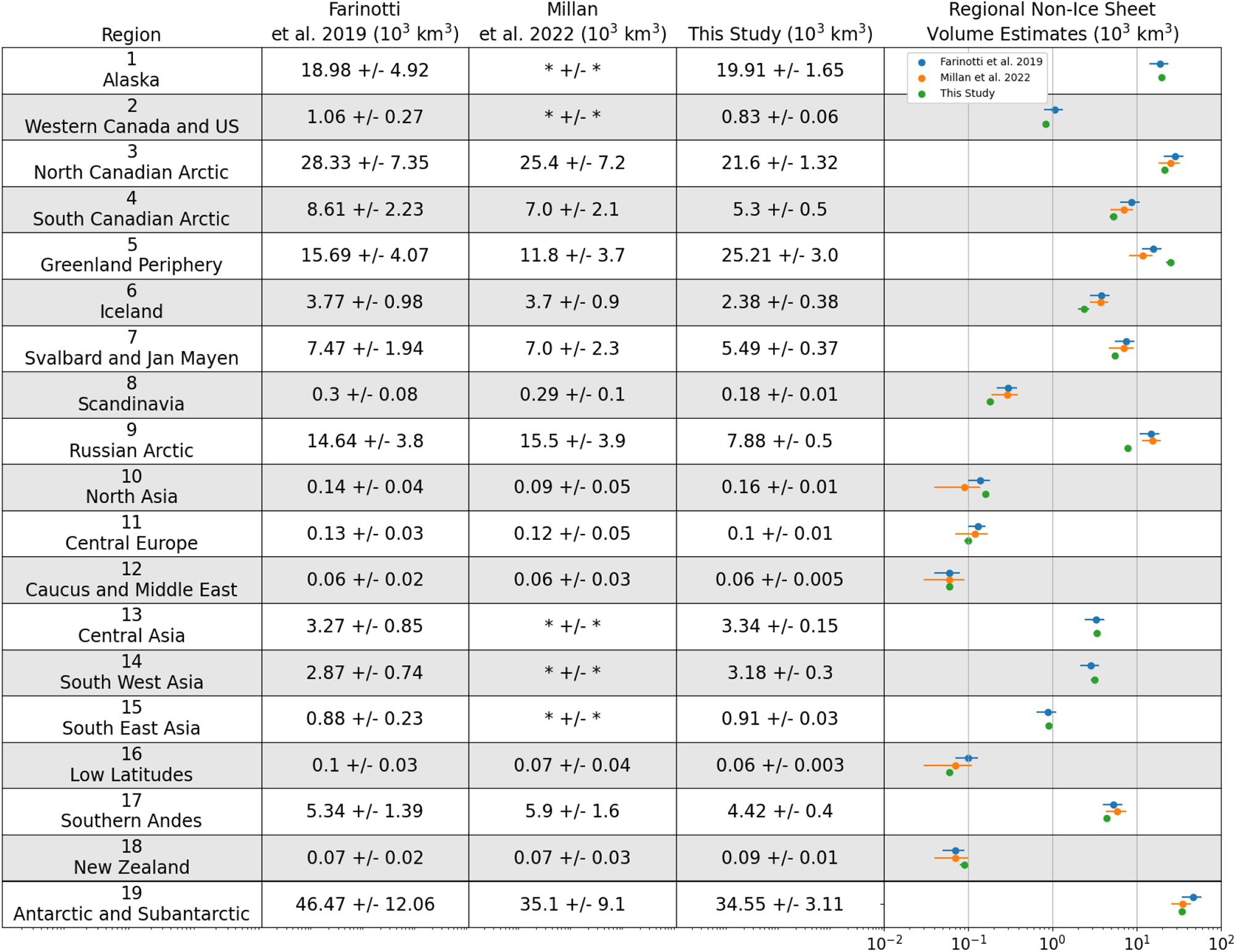
We interpret this difference as being due to the inadequate representation of water-terminating glaciers in our training dataset. The difference is due to a small number of glaciers: 70% of the difference between these models is explained by only 0.4% of glaciers in the RGI database (about 1000 individual glaciers). Of the 100 most negative volume differences, 42 are marine-terminating ice caps and 40 are ice shelf-supported glaciers near the Antarctic ice sheet. Regional variations, shown in Figure 2, show that our model exhibits the most significant negative biases in the Antarctic/Subantarctic (RGI region 19), the North Canadian Arctic (RGI region 2), Iceland (RGI region 6), Svalbard and Jan Mayen (RGI region 7) and the Russian Arctic (RGI region 9).
RGI regional volume comparisons between F19, M22 and this study. M22 combined Alaska and Western Canada (RGI 1, 2, respectively) into a single region, as well as high-mountain Asia (RGI regions 13,14,15) into a single region making it not possible to compare these regions. Discrepancies with M22 occur due to differing glacier domains (as noted by Hock and others, Reference Hock, Maussion, Marzeion and Nowicki2023). Comparisons with the underlying data are shown in the Supplementary Information.

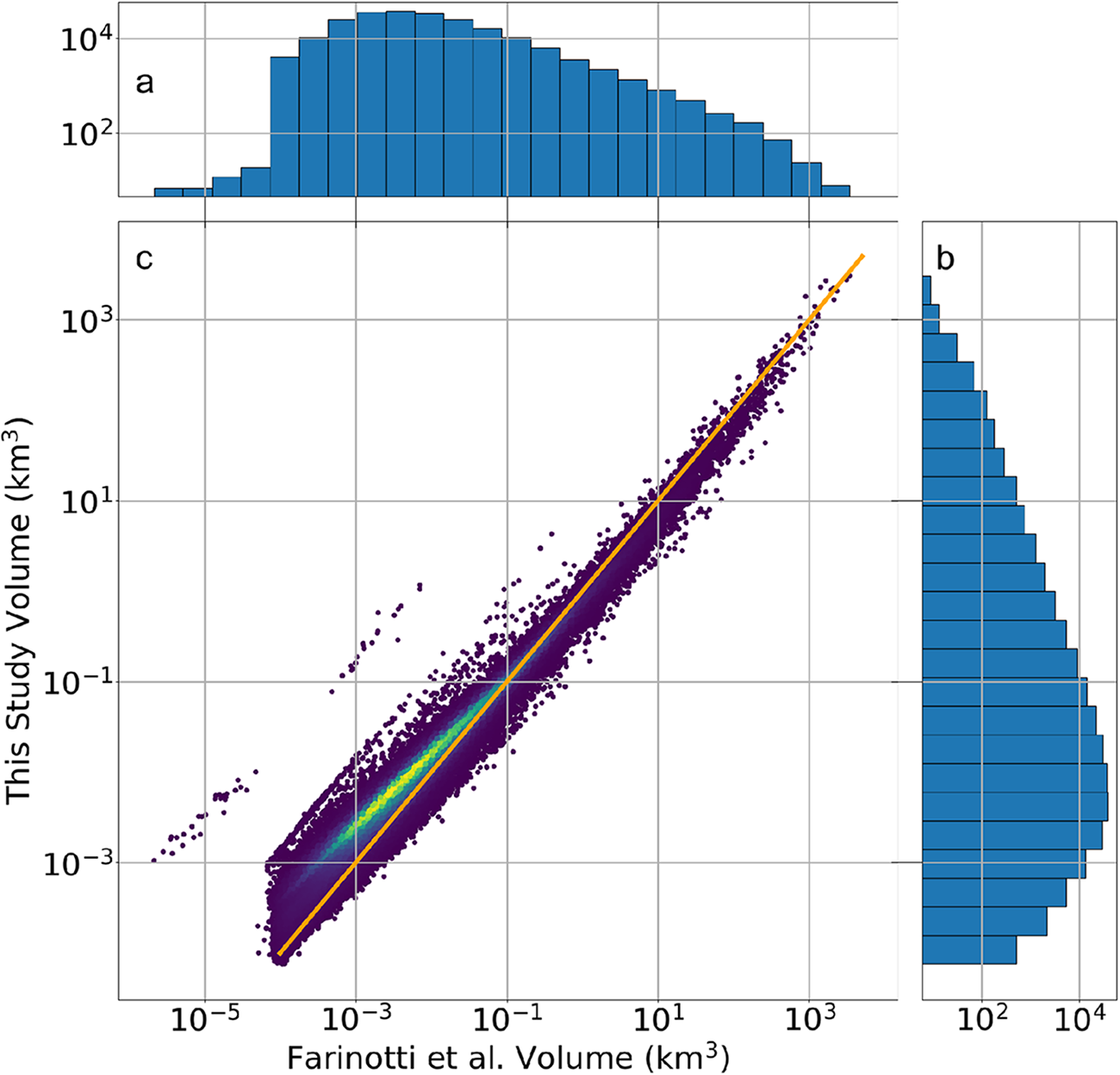
Our model makes comparable predictions to previously published global glacier volume estimates for glaciers that are not lake–terminating or ocean–terminating. Figure 3 compares our glacier volume estimates to those of F19 and Millan and others (Reference Millan, Mouginot, Rabatel and Morlighem2022), hereafter ‘M22’ for all glaciers in the RGI database. Our results are also similar in the distribution of glacier sizes, where we find that  $67\%$ of the global glacier volume is contained in just $0.2\%$ of the world’s glaciers (377 individual glaciers). Small glaciers with estimated volumes $ \lt 0.1$ km $^3$ show a slight positive difference in our model compared to F19, while volumes $ \gt 0.1$ km $^3$ show a slight negative difference compared to F19. Our model estimates regional glacier volumes that are largely within the confidence intervals of previous studies in regions with few water-terminating glaciers (Figure 2). We note that a handful of glaciers in Jan Mayen were estimated by F19 to be on the order of centimeters thick, which is interpreted as an artifact in that model (Figure 3).
(a) Histogram of volumes from Farinotti et al. 2019. (b) Histogram of volumes from this study. (c) Direct global comparison between volumes estimated by this study and that of Farinotti et al. 2019 on a log scale with one-to-one perfect fit in orange. Brighter colors represent the density of estimates. Summary statistics for our glacier volume estimates are given in Tables S1–S5.

4.2. Uncertainty quantification
We carry out a comprehensive analysis of sources of uncertainty in our calculations and find that the global glacier volume uncertainty  $\sigma^2$ can be approximated as, $\sigma^2 \approx A^2_k \text{Var}\left(\hat{H}_k\right)$, where the index $k$ refers to a particular glacier (with summation implied by the repeated indices), $A_k$ refers to the area of that glacier and $\hat{H}_k$ refers to its estimated thickness. The full expansion for $\sigma$ is given in the Methods.
Our analysis shows that global glacier volume uncertainty is predominantly controlled by glacier thickness rather than area (Methods). Of the terms that contribute to thickness uncertainty, we find that limited thickness observations are the dominant source of uncertainty (54% of the variance), followed by underlying measurement uncertainty (35%) and model misfit (11%). All other terms account for less than 0.05% of the variance. A statistical summary of these results is given in Figure S2 and Table S6.
On a glacier-by-glacier basis, we find that thickness uncertainty for the smallest glaciers can vary between 35% and 55%. Percent uncertainty decreases with increasing glacier size to roughly 10% for the largest glaciers. These results are presented graphically in Figure S4.
When comparing the confidence intervals between our study and F19, it is important to note that F19 used a heuristic approach to calculating these confidence intervals from regional uncertainty estimates. Specifically, F19 calculated their global confidence intervals as the sum of the standard deviations, rather than the sum of variances. While this approach results in a larger and more conservative uncertainty estimate, it does not preserve linearity for independent measurements. As a result, we note that F19 presented wider confidence intervals of  $\pm41 \times 10^3$ km $^3$ rather than the value that we quote of $\pm16 \times 10^3$ km $^3$ that arises from summing variances rather than standard deviations.
5. Discussion
Ice–ocean and ice–lake interactions are widely recognized as key controls on glacier dynamics, influencing calving rates, frontal melting and the force and mass balance at glacier termini (Benn and others, Reference Benn, Warren and Mottram2007). These processes are often observed to be sources of rapid change and potential instability, yet they also shape the equilibrium glacier geometry. In this study, we quantify the imprint of these interactions at the global scale by comparing models trained with and without water-terminating glaciers. We find that excluding ice–ocean and ice–lake interactions leads to a systematically lower estimate of global glacier volume, with the difference accounting for  $20\pm10$% of the total non-ice sheet global glacier volume. This result is consistent with the well-established role of ice shelves in buttressing grounded ice and supporting greater ice volumes in marine ice sheet systems (Rignot and others, Reference Rignot, Casassa, Gogineni, Krabill, Rivera and Thomas2004; Dupont and Alley, Reference Dupont and Alley2005; Gudmundsson, Reference Gudmundsson2013), but it also extends to water-terminating glaciers without ice shelves. Our findings therefore highlight that the presence of water at the ice front is a first-order control on the mean equilibrium state of glaciers.
Our conclusion that water-terminating glaciers are systematically thicker than land-terminating glaciers is consistent with both regional observations and theoretical considerations. In Svalbard, van Pelt and Frank (Reference van Pelt and Frank2025) found that glacier-averaged median thickness is about four times larger for tidewater glaciers (162 m) than for land-terminating glaciers (42 m). In High Mountain Asia, a population comparison indicates that lake-terminating glaciers are, on average, thicker over their ablation zones ( $\sim$110 m vs. $\sim$100 m) and especially near their termini (Pronk and others, Reference Pronk, Bolch, King, Wouters and Benn2021), complementing earlier work that documented contrasting geometry, thinning and retreat patterns by terminus type (King and others, Reference King, Dehecq, Quincey and Carrivick2018). From an inversion perspective, neglecting frontal ablation systematically underestimates both mass turnover and near-front thickness for marine-terminating glaciers, inflating regional underestimation of stored ice by $\sim$11–19% (Recinos and others, Reference Recinos, Maussion, Rothenpieler and Marzeion2019).
These empirical results align with height-above-buoyancy (HAB) considerations: water pressure at the ice front permits thicker termini than would be sustainable in air alone, setting a different boundary condition for equilibrium geometry (Nick and others, Reference Nick, van der Veen, Vieli and Benn2010; Bassis and Walker, Reference Bassis and Walker2012). Bassis and Walker (Reference Bassis and Walker2012) argued that Coulomb plastic fracturing limits the heights of subaerial ice cliffs to a height  $H_c\approx100$ m. Glaciers that terminate on land must therefore have terminus thickness $H(0) \lt H_c$. Glaciers that terminate in water instead must have terminus thickness $H(0) \lt H_w+H_c$ where $H_w \gt 0$ is the water depth. To illustrate the implications of this boundary condition, we consider an idealized glacier profile $H(x) = \sqrt{2x\tau/(\rho g) + H(0)^2}$, with gravitational acceleration $g$ and bed strength $\tau\approx100$ kPa. Equipped with this model, we find that a $20$ km long land-terminating glacier has an average thickness of 459 m, whereas a $20$ km long ocean-terminating glacier has an average thickness of 610 m, a difference of 33%. While research has often emphasized the role of ice cliff failure in rapid ice mass loss (Pollard and others, Reference Pollard, DeConto and Alley2015; DeConto and Pollard, Reference DeConto and Pollard2016), our analysis highlights the complementary point that water pressure at the ice front also supports thicker equilibrium termini. In this way, processes that might destabilize glaciers at short timescales can simultaneously shift their mean state toward larger volumes.
Forecasting models of glacier mass loss most often neglect ice–ocean interactions that are thought to be important for larger marine ice sheets. In the ensemble of models described by Marzeion and others (Reference Marzeion2020), for example, only one out of eleven models attempted to include ice–ocean interactions. Recent progress in the field has begun to place more emphasis on these processes (Recinos and others, Reference Recinos, Maussion, Rothenpieler and Marzeion2019; Malles and others, Reference Malles, Maussion, Ultee, Kochtitzky, Copland and Marzeion2023; Rounce and others, Reference Rounce2023). As water-terminating glaciers retreat and evolve into land-terminating systems, models that do not capture ice–ocean and ice–lake interactions may have limited ability to represent this transition. Our analysis thus provides new evidence that the boundary conditions at glacier termini fundamentally shape equilibrium thickness, with consequences for global ice volume and its sensitivity to climate forcing.
Data availability statement
All code is available with download links to data on GitHub and published through Zenodo: https://zenodo.org/records/11106415.
Supplementary material
The supplementary material for this article can be found at https://doi.org/10.1017/jog.2026.10123.
Acknowledgements
This manuscript improved because of discussions with David Rounce and Nathan Kutz.


 Open access