


1. Foreword by the Diabetes Steering Group on behalf of the Institute and Faculty of Actuaries
The Diabetes Steering Group (DSG), on behalf of the Institute and Faculty of Actuaries (IFoA), are delighted to introduce this paper, which, to our knowledge, is the first study that provides a comprehensive analysis of various mortality risk factors for individuals diagnosed with both Type 1 and Type 2 diabetes (Reid et al., Reference Reid, Oliver, Bagnall, Catchpole, Chadwick, Lambert, Li, Schneider, Tajapra, Yan and Zhou2023). This paper includes a model that provides the user with a mortality risk prediction for individuals living with and without diabetes.
This research is considered important to the primary audience, the UK insurance industry, as it furthers the DSG’s key research aim as set out in our initial paper (Reid et al., Reference Reid, Oliver, Bagnall, Catchpole, Chadwick, Lambert, Li, Schneider, Tajapra, Yan and Zhou2023); that is, to widen access to insurance products for customers living with diabetes by improving the insurance industry’s access to information on the specific mortality risk for those living with diabetes. The primary intended audience for this research is the actuarial community and insurance industry, specifically those insurers and reinsurers that write protection and longevity risk products in the UK. However, the IFoA has a Royal Charter under which the DSG also seeks to provide information for the wider public interest.
The Diabetes Working Party produced a sessional paper (Reid et al., Reference Reid, Oliver, Bagnall, Catchpole, Chadwick, Lambert, Li, Schneider, Tajapra, Yan and Zhou2023), published on 18th May 2023, which provided insights to diabetes mortality risk via a comprehensive literature review and a global underwriting survey. Following this, the working party sought to further the research aim by commissioning a research project. That research project is detailed herein and was commissioned by the IFoA Actuarial Research Centre (ARC) and a group of industry participants, specifically Pacific Life Re, Partner Re, Swiss Re, Legal & General and Zurich Insurance Group. The research was carried out by world-leading experts in risk analysis, risk modelling and risk evaluation at the University of Leicester, namely Dr Bogdan GrechukFootnote 1 , Dr Evgeny Mirkes and Prof Alexander Gorban. These academic researchers are supported by the Real World Evidence Centre and the Leicester Diabetes Centre, a unique, collaborative partnership between the NHS and the University of Leicester.
Individuals with diabetes, both Type 1 and Type 2, run a greater risk of developing one or more severe health complications, including cardiovascular and cerebrovascular disease. Diabetes is also a leading cause of blindness in working-aged individuals and a common cause of kidney failure. Life expectancy following a diagnosis of diabetes has historically been lower than in those without diabetes, given that inadequate glycaemic control gives rise to several complications that cause premature death, along with increased risks of long-term disability.
In recent years, early detection and management of diabetes, both from a personal as well as a physician-led perspective, has improved such that survival with diabetes has increased. New pharmaceuticals, coupled with enhanced monitoring and modern insulin dosage systems, have transformed the lives of individuals living with diabetes. Life expectancy with optimal glycaemic management has been extended in those with diabetes, but the long-term impact of new pharmaceuticals has yet to be fully appreciated.
The overarching aim of the research project is to develop a deeper understanding of the mortality risk associated with a diagnosis of Type 1 and Type 2 diabetes and the impact of recent improved medical treatments. More specifically, the DSG’s objectives are to:
-
• Gain insights from recent data by considering advanced data analytic techniques to understand relative mortality risk factors and interactions.
-
• Produce a model that can predict mortality across a wide age range at a granular level for lives living with and without both Type 1 and Type 2 diabetes. The model should include co-morbidities such that the impact on mortality of living with and without diabetes in the presence of a wide range of co-morbidities can be understood.
The work carried out by the University of Leicester is detailed within this paper: background on the data sources used, for example, Clinical Practice Research Datalink (CPRD) and linked data; the process of data ingestion and cleaning; the data analysis; and the fitting of a Cox proportional hazards model. The DSG sought a transparent model where inferences can be drawn, and therefore a regression model was selected, namely the Cox proportional hazards model. The DSG built an accompanying Shiny applicationFootnote 2 so that the insurance industry and any interested wider stakeholders, for example, Diabetes associations and general practitioners (GPs), can interact with the model output.
The DSG is satisfied that the research outputs have been carried out to a high quality and in line with expectations to produce findings that are relevant to the primary intended audience (e.g., the actuarial community and insurance industry).
The interactive Shiny application will enable the user to consider the impact of different attributes on a general sample population, as well as a population of diabetes Type 1 and Type 2. The DSG would like to draw the reader’s attention to the benefits and limitations in Section 6.6 and to advise that care be exercised when interpreting results and utilising the Shiny application. Section 7 includes a general industry discussion followed by an applied industry discussion. The modelling was appreciated in the general discussion but there are many complications such as the quality of the data and how to handle co-morbidities correctly. Building a general model that covers Type 1 and Type 2 for all the different co-morbidities was ambitious and we understand this is the first time that has been done. The general feedback was that creating a model based on CPRD data was worthwhile as an initial approach that can be improved in future based on the feedback from practitioners.
1.1 Data Used
This study is based in part on data from the CPRD obtained under licence from the UK Medicines and Healthcare products Regulatory Agency. The data is provided by patients and collected by the NHS as part of their care and support. The interpretation and conclusions contained in this study are those of the author(s) alone.Footnote 3 We also used linked Hospital Episode Statistics (HES) data and Office for National Statistics (ONS) mortality data.
2. Introduction
2.1 Background
Both Type 1 and Type 2 diabetes are serious diseases and there has been a dramatic increase in prevalence over the last few decades. The number of worldwide cases has quadrupled between 1980 and 2014 (NCD Risk Factor Collaboration (NCD-RisC), 2016) and has increased for both Type 1 and Type 2 diabetes (Patterson et al., Reference Patterson, Karuranga, Salpea, Saeedi, Dahlquist, Soltesz and Ogle2019). More than half a billion individuals are living with diabetes worldwide as of 2021, and this number is predicted to grow to 1.3 billion in the year 2050 (GBD 2021 Diabetes Collaborators, 2023). Over 300 million individuals have prediabetes (International Diabetes Federation, 2015) and it is estimated that almost half of all individuals ( $49.7{\rm{\% }}$
) living with diabetes are undiagnosed (Cho et al., Reference Cho, Shaw, Karuranga, Huang, da Rocha Fernandes, Ohlrogge and Malanda2018).
$49.7{\rm{\% }}$
) living with diabetes are undiagnosed (Cho et al., Reference Cho, Shaw, Karuranga, Huang, da Rocha Fernandes, Ohlrogge and Malanda2018).
In the UK, the number of individuals living with diabetes in all its forms is approaching 5 million, and this number is predicted to rise to 5.5 million by 2030 (Cho et al., Reference Cho, Shaw, Karuranga, Huang, da Rocha Fernandes, Ohlrogge and Malanda2018). The expected lifetime of an individual with diabetes is significantly lower than for non-diabetic individuals of similar age and other conditions (Bertoni et al., Reference Bertoni, Krop, Anderson and Brancati2002; Tancredi et al., Reference Tancredi, Rosengren, Svensson, Kosiborod, Pivodic, Gudbjörnsdottir, Wedel, Clements, Dahlqvist and Lind2015). The analysis of diabetes-related mortality is complicated by the fact that individuals rarely die from diabetes directly. Instead, individuals with diabetes have increased risk of death from other diseases (DeFronzo, Reference DeFronzo2009). In the last decade, significant advances in medical treatments for Type 1 (Boscari & Avogaro, Reference Boscari and Avogaro2021) and Type 2 (Chee & Dalan, Reference Chee and Dalan2024) diabetes seem to have reduced the mortality risk for many individuals. However, the effect of these treatments on mortality risk is not yet fully understood. Studies to date that provide information on mortality risk for individuals with diabetes are derived from data ten or more years old that do not reflect those more recent treatments.
2.2 Overview of this Research Project
This research project develops models for mortality prediction for individuals with Type 1 and Type 2 diabetes. These models are based on recent data (namely the years 2010–2019) and as such include the impact of recent treatments. The model output is mortality predictions for an individual based on risk factors including age, gender, body mass index (BMI), blood pressure (BP), cholesterol level (CL), smoking status, index of multiple deprivation (IMD), blood glucose (sugar) level (HbA1c), duration since diabetes diagnosis and existence of various co-morbidities. With this information on each risk factor as an input, the models provide an output of a probability of death for the individual within the next t years for any given $t \gt 0$
. To compute this probability, the models allow for the effect of the risk factors, listed above, both separately and for some of the factors in combination. For example, coronary heart disease significantly increases the mortality risk for all individuals with diabetes, but the increase is particularly strong for individuals with high BMI.
$t \gt 0$
. To compute this probability, the models allow for the effect of the risk factors, listed above, both separately and for some of the factors in combination. For example, coronary heart disease significantly increases the mortality risk for all individuals with diabetes, but the increase is particularly strong for individuals with high BMI.
It is important to note that this analysis does not attempt to draw causal epidemiological conclusions. Instead, it seeks to pinpoint risk factors that are reliably correlated with mortality in the diabetic population. Such an approach reflects the requirements of underwriting practice, which relies on consistent and interpretable risk differentiators to support equitable, evidence-driven decisions.
The analysis of data in this research project, alongside the existing literature (Huxley et al., Reference Huxley, Peters, Mishra and Woodward2015; Kautzky-Willer et al., Reference Kautzky-Willer, Leutner and Harreiter2023) reveals many risk factors that correlate with mortality differently depending on whether the diagnosis is of Type 1 or Type 2 diabetes, and with gender. Therefore, separate mortality models were developed by gender for (i) the general population, (ii) individuals living with Type 1 diabetes and (iii) individuals living with Type 2 diabetes. There are therefore six models produced in total.
All of the models are Cox proportional hazards models (Cox, Reference Cox1972). A major advantage of this model is that the computed Cox coefficients explicitly show the effect of each factor on the mortality risk. The primary audience, the insurance industry, is required by regulation to have transparency in pricing terms and as such a transparent model where inferences can be drawn was preferred.
These models can be used to inform the insurance industry on the specific mortality risk posed by individuals with diabetes with the aim of achieving availability of insurance products for those living with diabetes and also more appropriate pricing and reserving for life and health insurance products. These models provide a better understanding of the mortality risk factors for individuals with diabetes which may also be of interest to wider stakeholders.
2.3 Comparison with the Existing Literature
The literature on diabetes is very rich. However, many studies investigate the effect of only one or at most several risk factors. Indeed, each risk factor considered herein can be found in the existing research as it affects the prevalence of diabetes or the associated health outcomes including: age (de Miguel-Yanes et al., Reference de Miguel-Yanes, Shrader, Pencina, Fox, Manning, Grant, Dupuis, Florez, D’Agostino, Cupples and Meigs2011; Constantino et al., Reference Constantino, Molyneaux, Limacher-Gisler, Al-Saeed, Luo, Wu, Twigg, Yue and Wong2013), gender (Ohkuma et al., Reference Ohkuma, Komorita, Peters and Woodward2019; Mauvais-Jarvis, Reference Mauvais-Jarvis2018), ethnicity (Goff, Reference Goff2019), physical activity (Wahid et al., Reference Wahid, Manek, Nichols, Kelly, Foster, Webster, Kaur, Friedemann Smith, Wilkins, Rayner, Roberts and Scarborough2016), BMI (Chatterjee et al., Reference Chatterjee, Khunti and Davies2017), alcohol consumption (Baliunas et al., Reference Baliunas, Taylor, Irving, Roerecke, Patra, Mohapatra and Rehm2009), socio-economic status (SES) (Evans et al., Reference Evans, Newton, Ruta, MacDonald and Morris2000) and co-morbidities such as cardiovascular disease (Leung et al., Reference Leung, Eurich, Lamb, Majumdar, Johnson, Blackburn and McAlister2009; Wilmot et al., Reference Wilmot, Edwardson, Achana, Davies, Gorely, Gray, Khunti, Yates and Biddle2012; Riley & Cowan, Reference Riley and Cowan2014; Stamler et al., Reference Stamler, Vaccaro, Neaton and Wentworth1993), heart failure (Ohkuma et al., Reference Ohkuma, Komorita, Peters and Woodward2019), coronary heart disease (Peters et al., Reference Peters, Huxley and Woodward2014), stroke (Emerging Risk Factors Collaboration, 2010), hypoglycaemia (Elwen et al., Reference Elwen, Huskinson, Clapham, Bottomley, Heller, James, Abbas, Baxter and Ajjan2015), high BP (Chiriacò et al., Reference Chiriacò, Pateras, Virdis, Charakida, Kyriakopoulou, Nannipieri, Emdin, Tsioufis, Taddei, Masi and Georgiopoulos2019), depression (Ali et al., Reference Ali, Stone, Peters, Davies and Khunti2006), dementia (Bello-Chavolla et al., Reference Bello-Chavolla, Antonio-Villa, Vargas-Vázquez, Ávila-Funes and Aguilar-Salinas2019), fatty liver disease (Song et al., Reference Song, Jia, Li, Wang, Ren and Chen2021) and Covid-19 (Hussain et al., Reference Hussain, Bhowmik and do Vale Moreira2020; Pal & Bhadada, Reference Pal and Bhadada2020) (non-exhaustive list).
In contrast, this project builds a model that allows for many risk factors, separately and, for some of the factors, in combination. Such studies are far less common in literature. Jensen et al. (Reference Jensen, Moseley, Oprea, Ellesøe, Eriksson, Schmock, Jensen, Jensen and Brunak2014) developed a clustering methodology that can be used to identify new risk factors related to diabetes. Golovenkin et al. (Reference Golovenkin, Bac, Chervov, Mirkes, Orlova, Barillot, Gorban and Zinovyev2020) studied a selection of more than 100,000 hospitalisation cases with individuals suffering from diabetes characterised by 55 attributes. The outcome of interest was hospital readmission, rather than mortality.
To the best of our knowledge, none of the existing recent literature provides a comprehensive analysis of the impact of various risk factors on the mortality of individuals living with diabetes. In addition, the literature does not provide a general model for mortality prediction for individuals with and without diabetes based on a large variety of risk factors. Herein, this is the focus of this research.
3. Data Structure
3.1 Data Collection
This research requires information regarding the outcome of interest - death. It also requires information regarding possible risk factors for that outcome of interest, such as diabetes diagnosis type and date, age, gender, etc. The first was sourced using the ONS Death Registration Data, which enables a status of alive or deceased to be mapped to an anonymised individual record, and, in the latter case, the date of death. The second was sourced using the CPRD database (Herrett et al., Reference Herrett, Gallagher, Bhaskaran, Forbes, Mathur, Van Staa and Smeeth2015), which contains anonymised individual data records from a network of general practices (GP) across the UK. In addition, information from the HES database was utilised to gain further information on co-morbidity diagnosis from the National Health Service (NHS) hospitals’ admissions and outpatient appointments data. Deprivation is considered a significant risk factor for mortality (Evans et al., Reference Evans, Newton, Ruta, MacDonald and Morris2000). To allow for this, an IMD score was mapped at a GP and at an individual level.
These data sets and the linkage of these data sets were necessary to enable the influence of various risk factors on the mortality of those living with diabetes to be understood. Samples of the full database were taken over a restricted time and geographical scope in order to work with the least amount of data to achieve the research aim. This approach aligns with the principle of data minimisation, ensuring that only the minimum amount of data necessary to adequately address the research question was used, thereby reducing computational burden and safeguarding data privacy. These data sets are fully anonymised, intended for use by researchers and their use in this project was approved by CPRD in 2021.
The time period for this research spans from 1 January 2010 (the “study start date”) to 31 December 2019 (the “study end date”). This was the most recent 10-year period that was not impacted by the Covid-19 pandemic. Although some of the data sets are UK wide, the HES data is restricted to England and as such, the geographical scope of the research was narrowed to England as this linkage was necessary to understand the influence of co-morbidities on the mortality of diabetes patients. Data from the private healthcare system is not included; this is not considered material because the vast majority of diabetes care and associated hospital admissions in England occur within the NHS, making NHS HES a comprehensive and representative source for the population under study.
The following samples were requested from the CPRD database:
-
• A diabetes sample: anonymised individual records from the database who have at least one record related to diabetes (Type 1 or Type 2), were alive at the study start date and were at least 18 years of age by that date (i.e., a year of birth is 1991 or earlier). This sample resulted in 621,115 individual records. Given that approximately 4 million adults in England were living with diabetes (diagnosed and undiagnosed) in 2019, about 15% of them were included in this sample.
-
• A general sample: a random sample of 250,000 anonymised individual records, regardless of diabetes status (i.e., general) who were alive and were at least 18 years of age at the study start date. This sample is about $0.5{\rm{\% }}$
of the relevant population.
$0.5{\rm{\% }}$
of the relevant population. -
• An additional sample: a random sample of 25,000 anonymised individual records, regardless of diabetes status, with any of the following diseases: heart failure, coronary heart disease, angina, heart attack, stroke, amputation, macrovascular disease, asthma, atrial fibrillation, cancer, chronic kidney disease (CKD), chronic obstructive pulmonary disease (COPD), dementia and epilepsy.

These samples are not mutually exclusive and as such, some records appear in several samples. In total, $1,205,657$
unique records were selected across the three samples. This is referred to herein as the “total data set”.
$1,205,657$
unique records were selected across the three samples. This is referred to herein as the “total data set”.
For each individual record in the total data set, the following were sought:
-
• The entire medical record available in CPRD.
-
• The HES data for that record linked.
-
• The ONS Death registration data for that record linked.
-
• The IMD mapped at an individual and GP level.
3.2 CPRD Data
The CPRD data arrived in the following tables: Patients, Practice, Staff, Consultation, Clinical, Additional Clinical Details, Referral, Immunisation, Test and Therapy (9 tables in total referred to herein as the “main tables”), plus additional tables without necessary information (referred to herein as “ignored tables”). The list of ignored tables is presented in Table 12.
Each table has its own set of columns of various lengths. The first column is Patient Identifier (“patid”), which is an encrypted unique identifier given to an individual record in the CPRD data set. All tables and figures can be found in the separate “Tables and Figures” document. Table 1 provides a list of columns and their description. The field patid is used to find records in all tables that correspond to a given individual record. Other forms of linkage are provided. Tables 1–10 describe all columns in the main tables, together with all forms of linkage. For convenience, links between fields are also summarised in Table 11 and Figure 1.
There are also two additional dictionary tables, “Medical dictionary” and “Product dictionary”. The diseases in CPRD tables are encoded using Read version (v) 2 codes also known as “Medcodes”, for example, Heart failure has Medcode “G58.00”. A list of Medcodes with descriptions of the corresponding medical terms is presented in the Table “Medical dictionary” and products (e.g., prescribed drugs) are encoded using “prodcodes”. Table “Product dictionary” lists all such drugs and their descriptions. Refer to Tables 13 and 14 for column descriptions in the dictionary tables.
3.3 Data from Linked Sources
The linked data from HES are organised into 11 tables: patients, hospitalisations, episodes, diagnoses by episode, diagnoses by hospitalisation, primary diagnoses across a hospitalisation, procedures, augmented care periods, critical care, maternity and health resource group. See Tables 15–25 for the descriptions of all table columns. For this research, only the first 6 tables were necessary as these contain information about diagnoses. All tables contain the column “patid” to assist in linkage. Individual patients may contribute data to more than one GP practice. In this case, multiple patid’s may represent the same individual. However, a column “gen hesid” within the table “Patients” in the HES data provides a CPRD generated unique key which allows information in CPRD tables and in HES tables to be identified where it refers to the same individual. Within the total data set, there were 15,107 cases that had multiple patid’s.
The information about diagnosis in HES is recorded using the International Classification of Diseases version 10 (ICD-10) coding frame. This differs from the CPRD’s medcodes, for example, Heart failure has Medcode “G58.00” while the corresponding ICD-10 code is “I50.9”. For this reason, a mapping between ICD-10 codes and medcodes was required (NHS Digital, 2018).
The linked ONS Death registration data consists of only one table. It contains the required information of patid, date and cause of death. A full list of columns is shown in Table 26.
The IMD data consists of two files: one contains a dictionary to identify the GP county, and another the deprivation score at the individual and GP level. A description of the columns is shown in Table 27.
Not all individuals in the total data set are “eligible” for the linked data: HES, ONS and IMD. There is a text document linkage eligibility named “new patids.txt” that specifies which individuals are “eligible” for linked data. Individuals eligible for HES linked data have the attribute “hes e” equal to 1. Similarly, individuals eligible for ONS linking have “death e” equal to 1, while individuals eligible for IMD linking have “lsoa e” equal to 1.
4. Data Treatment and Missing Data Analysis
4.1 Information Required for Mortality Risk Analysis
The selection of variables for this study was informed by a combination of evidence from the academic literature (as discussed in Section 2) and established actuarial practice within the insurance industry. Many of the included factors, such as age, gender, smoking status, BMI and indicators of co-morbid conditions, have consistently been associated with variations in mortality risk among individuals with diabetes. These are widely recognised both in clinical studies and in underwriting guidelines as relevant indicators of long-term health outcomes. Additionally, variables such as BP, CLs and HbA1c were included based on their routine use in risk stratification and premium setting by insurers, where actuarial judgement and historical claims experience inform expectations of mortality risk, even in the absence of strong causal evidence. As mentioned in Section 2.2, the objective of this analysis is not to establish epidemiological causation, but rather to identify variables that show meaningful correlations with mortality outcomes within the diabetes population. This distinction aligns with the practical needs of insurance underwriting, where the goal is to detect consistent, interpretable differentiators in mortality risk that can support fair and evidence-based decision-making.
The following data items are available across the linked data. The aim of data treatment was therefore to produce a data table, where each individual (patid) has the following information, which is appropriately cleaned and suitable for analysis:
-
• Outcome of interest:
-
• Individual’s status as alive or deceased as at study end date 31/12/2019.
-
• Date of death, where applicable.
-
-
• Mortality risk factors of interest:
-
• Static data items.
-
• Age at the start date.
-
• Gender.
-
• IMD.
-
• Smoking status.
-
-
-
• Regularly recorded data items.
-
• Body mass index (BMI).
-
• Blood pressure (BP).
-
• Cholesterol level (CL).
-
• Blood glucose (sugar) level (HbA1c).
-
• Indicator for diagnosed diseases which are considered “potentially significant” (see Table A). We emphasise that this is the original list of “potentially significant” diseases for the mortality of individuals with diabetes. This list was formed based on the literature review (Section 2) and consultations with specialists from Leicester Diabetes Research Centre. We do not claim that all these diseases are indeed significant. In fact, identification of a subset of significant diseases is a major part of this research project.
Table A.List of abbreviations used for medical conditions
Table A Long description
A table listing abbreviations for medical conditions related to Type 1 and Type 2 diabetes. The table has two columns: one for Type 1 diabetes abbreviations and one for Type 2 diabetes abbreviations. Each row lists a condition and its corresponding abbreviation. For Type 1 diabetes, conditions include atrial fibrillation (AF), amputation (Amp), anorexia (Ano), asthma (Ast), bronchiectasis (Bro), cancer (Can), chronic sinusitis (CS), cystic fibrosis (CyF), dementia (Dem), epilepsy (Epi), hearing loss (HeL), hypertension (Hyp), learning disabilities (LD), macrovascular disease (MVD), prostate disorders (PrD), pulmonary fibrosis (PuF), schizophrenia (Sch), stroke (Str), and thyroid disorders (ThD). For Type 2 diabetes, conditions include acquired immune deficiency syndrome (AID), angina (Ang), anxiety (Anx), blindness (Bli), coronary heart disease (CHD), chronic liver disease (CLD), cryptogenic organizing pneumonia (COP), diverticular disease of intestine (DDI), depression (Dep), hemiplegia (Hem), heart failure (HF), irritable bowel syndrome (IBS), mild liver disease (MLD), multiple sclerosis (MSc), psoriasis or eczema (PsE), peptic ulcer disease (PUD), rheumatoid arthritis (RhA), moderate or severe liver disease (SLD).
-
• Date of diagnosis, where applicable.
-

The following data items, although available across the linked data and considered potential risk factors of interest, were not included for analysis for the reasons shown below.
-
• Marital status – high level of missing data.
-
• Ethnicity – high level of missing data and not used by the UK insurance industry.
Sections 4.2 and 4.3 provide insights for each item of data used including commentary on missing data analysis where relevant and data treatment. Further commentary can be found alongside the relevant tables within the “Tables and Figures” document.
4.2 Data for Outcome of Interest
There are two potential sources of date of death: “deathdate” field in the original CPRD data and “ONSDeath” field in the linked ONS data. For some individuals there are discrepancies in these fields. Some individuals have different dates of death (see Table 46) and there are $86,{\rm{\;}}825$
records with an ONS date of death without a “deathdate” in the CPRD data (this is 16% out of the total of
$86,{\rm{\;}}825$
records with an ONS date of death without a “deathdate” in the CPRD data (this is 16% out of the total of $543,{\rm{\;}}668$
individuals in the total sample linked in ONS). The lack of any recorded activities (such as GP visits, hospitalisations, etc.) after the ONS date of death is considered adequate evidence that the ONS date of death is correct. Within the insurance industry, the ONS data is considered the “gold standard” for death records and this is supported in the literature (Gallagher et al., Reference Gallagher, Dedman, Padmanabhan, Leufkens and de Vries2019).
$543,{\rm{\;}}668$
individuals in the total sample linked in ONS). The lack of any recorded activities (such as GP visits, hospitalisations, etc.) after the ONS date of death is considered adequate evidence that the ONS date of death is correct. Within the insurance industry, the ONS data is considered the “gold standard” for death records and this is supported in the literature (Gallagher et al., Reference Gallagher, Dedman, Padmanabhan, Leufkens and de Vries2019).
All individuals who died before the study start date are removed. To ensure that individuals with deaths pre-dating the ONS death register’s creation in 1998 are not included within the study period, the CPRD date of death is used if it is before 1998. For deaths after 1998 the ONS death data is used.
The CPRD date of death is considered fit for the filtering purpose above but is not considered fit for the purpose of mortality analysis. Therefore, where a link between the ONS and CPRD data cannot be established, these cases are removed from the study. That is, only individuals with ONS linked data are used. Although, this reduces all sample sizes it is considered appropriate because the CPRD date of death information is considered to be unreliable for mortality analysis. In the diabetes sample, there were 621,115 individuals initially. A link can be established to the ONS for 283,057 (45%). Excluding those individuals who died before the study start date, the sample contains 242,461 individuals (85%). In the general sample, there were 250,000 individuals initially. A link can be established to the ONS for 103,597 (41%). Excluding those individuals who died before the study start date, the sample contains 95,786 individuals (92%). These data are summarised in Table B.
-
• The effect of excluding non-ONS linked individuals is compared between the initial sample (all individuals) and the linked sample (only individuals linked with ONS). Standard tests for statistical significance such as the Kolmogorov–Smirnov test (KS test) are not useful for large data sets.Footnote 4 Therefore, a manual threshold is introduced. A 1% difference in fractions for linked and non-linked subsamples is considered a sufficient effective size. The impact of filtering needs to be considered by the main variables of interest for mortality analysis including gender, age and co-morbidities.
-
• Table 47 shows the contingency of gender from the initial to the linked sample. Female individuals comprise
$47.8{\rm{\% }}$
of the initial sample and
$47.6{\rm{\% }}$
of the linked sample. The change in the composition of the samples, that is, the effect size is
$0.2{\rm{\% }}$
. Because this is less than 1%, it can be assumed that linking and gender are independent. -
• Figure 3 presents the contingency of age from the initial to the linked sample. The age distributions are similar and the mean age is
$59.79$
for the initial sample and
$60.82$
for the linked sample. The difference in mean age is nearly 1 year, which is considered negligible alongside the similar age distribution. -
• Table 48 presents a comparison of various diseases associated with the individuals in the initial and the linked sample. Most of the diseases (28 out of 41) show statistically significant differences in prevalence between the initial and the linked samples, indicating that linkage to the ONS is not independent of disease status for these conditions. This suggests that certain co-morbidities may affect the likelihood of successful linkage, potentially due to systematic differences in healthcare usage or death registration practices associated with specific conditions. As a result, this introduces the possibility of selection bias in analyses relying solely on the linked sample. While the effective sizes for many of these conditions remain modest, this dependency needs to be acknowledged in any inference about disease-related mortality risks to avoid over- or underestimating effects due to differential linkage rates.


Sample sizes before and after ONS linkage

Table B Long description
The table presents data on sample sizes before and after linkage to the Office for National Statistics (ONS) for diabetes and general samples. It consists of two rows and four columns. The columns are labeled Sample type, Initial individuals, Linked to ONS (percentage), and Alive at study start (percentage). The diabetes sample initially had 621,115 individuals, with 283,057 (45 percentage) linked to ONS, and 242,461 (85 percentage) alive at the study start. The general sample initially had 250,000 individuals, with 103,597 (41 percentage) linked to ONS, and 95,786 (92 percentage) alive at the study start. The table highlights the reduction in sample sizes due to the linkage process and the proportion of individuals alive at the study start.
A careful investigation of the database reveals the existence of some individuals of old age that are linked to ONS, have no death date records, but also have no recorded GP activity after the study start date. We suspect that these individuals are in fact deceased or emigrated and no longer residing within the UK,Footnote 5 and performed a more careful investigation.
Of the $1,205,657$
records within the total sample:
$1,205,657$
records within the total sample:
-
• 53,045 records have an age at the study start date of at least 80.
-
• According to CPRD data, 33,079 were alive at the study start date.
-
• According to the ONS linked data, 8,566 of the above were linked to ONS and alive at the study end date.
-
• The overlapping cases from the above two data sets indicated as “alive” are 8,347.
For those 8,347 “alive” individuals, we then search for test dates and diagnosis dates, and we have discovered that
-
• 1,353 individuals have the last date of diagnosis before the study start date.
-
• 1,884 individuals have the last date of test before the study start date.
-
• In total, there are 1,251 individuals without any recorded GP activity after the study start date.
Table 49 shows the age distribution for the samples before and after removing those individuals. In particular, there are 5 individuals older than 120 with no death date records, and all 5 cases have no GP recorded activity after the study start date. It is unlikely that individuals alive at these ages are no longer interacting with the registered GP. It was considered likely that these individuals were deceased, but the death was not recorded. This may occur where an individual emigrated from the UK some time ago. On this basis, all records with an age greater or equal to 80 at the study start date, which do not have any GP recorded activity after the study start date, are removed from the analysis.
The removal of the above 1,251 individuals, who we call “fake” individuals, has a crucial effect on the research objective, especially in insurance context. While the proportion of these individuals in the entire database is negligible (1,251 out of $1,205,657$
, which is about
$1,205,657$
, which is about $0.1{\rm{\% }}$
), their proportion among 8,347 individuals of age 80+ linked to ONS is 15%. This percentage increases when we increase age threshold and reaches 100% for the individuals aged 110+. Therefore, if “fake” individuals were not excluded, they would lead to a severe underestimation of the mortality rate at old ages.
$0.1{\rm{\% }}$
), their proportion among 8,347 individuals of age 80+ linked to ONS is 15%. This percentage increases when we increase age threshold and reaches 100% for the individuals aged 110+. Therefore, if “fake” individuals were not excluded, they would lead to a severe underestimation of the mortality rate at old ages.
After removing these individuals, the number of individuals left in the total sample who are linked to ONS is 656,410. All the statistics for the total sample described below are based on this set of individuals.
4.3 Data for Mortality Risk Factors of Interest
The following data were processed as either static or regularly monitored.
4.3.1 Static Data Items
The following data items are considered static and therefore extracted from the data as at the study start date. Although some items may vary through the study period, such changes are not considered materially significant for the purposes of mortality modelling. For instance, occasional corrections to recorded date of birth or gender are rare and typically reflect data quality improvements rather than actual changes in the individual’s characteristics. In the context of this study, where the objective is to evaluate broad mortality risk patterns across a large population, treating these variables as fixed at the study start date simplifies the analysis without introducing meaningful bias. This assumption aligns with industry practice in insurance risk modelling, where underwriting is typically based on characteristics known at a specific point in time.
4.3.1.1 Age and Gender
Age is defined as the number of full years of age at the start of the study. It has been computed as 2009 minus the year of birth. In Cox proportional hazards model, we will also have a parameter t that represents time from the study start. The age at any moment can then be computed as $A + t$
, where A is the age at the study start. Having A as a constant simplifies the analysis.
$A + t$
, where A is the age at the study start. Having A as a constant simplifies the analysis.
Gender is recorded as a binary value: 1 – for Male, 2 – for Female, as recorded at birth.
4.3.1.2 IMD
IMD takes an integer value from 1 to 10 and is computed based on the postcode recorded at the study start. For individual records, the data item “IMD decile” is missing for nearly 58% of the total sample and nearly 61% of the general sample. In these cases, the missing value is imputed with the IMD for the individual’s registered GP. The remaining missing values (291 cases – 171 of which have the IMD recorded as 0 and 120 for which it is recorded as NaN) are allocated a value 5, which is a middle value for the index.
We acknowledge that the proportion of missing individual-level IMD data is substantial and that GP catchment areas are geographically broader than individual postcodes. However, excluding these records would result in a loss of over half the study population, drastically reducing statistical power and likely introducing significant selection bias, as data missingness is rarely random. Consequently, we utilised the GP-level IMD as a pragmatic proxy, operating on the reasonable assumption that patients generally register with a GP practice in close proximity to their residence, thereby sharing similar socio-economic characteristics.
4.3.1.3 Smoking Status
Files Smoke_ent_*.txt contain information about smoker status (1 – Yes, 2 – No, 3 – Ex smoker). From Smoke_ent_*.txt we received $12,511,090$
records. After removing records with value 0 “Data Not Entered” we have
$12,511,090$
records. After removing records with value 0 “Data Not Entered” we have $12,509,309$
records. After removing duplicate records, we have
$12,509,309$
records. After removing duplicate records, we have $11,068,831$
records.
$11,068,831$
records.
These files should be accompanied by Smoke_Clin_*.txt to identify dates. There were 10,714 records with missing event dates. These dates were substituted by system date, which is the date the record was made in the database.
In addition, files Smoke_Int_*.txt and Smoke_test_*.txt present smoking information using medcodes. ICD-10 codes and medcodes for smoker status are presented in Table 35. The total number of records from files Smoke_Int_*.txt, Smoke_test_*.txt and Smoke_diag.txt is 16,248. After removing all of records with medcodes unrelated to smoking status we have 4,107 records.
In the total data set we have 75,727 individuals, or $6.7{\rm{\% }}$
, without smoker status recorded. In the general sample, this applies to 50,080 individuals, or
$6.7{\rm{\% }}$
, without smoker status recorded. In the general sample, this applies to 50,080 individuals, or $21.6{\rm{\% }}$
. The results of the analysis of the randomness of missingness are presented in Table 36. They show that values are not missing completely at random. This means that we cannot remove records with missing values, and so we should impute the data. The imputation method we used was to set the value “Non-smoker” for records without smoker status. This approach is based on the heuristic of clinical coding practices, where positive risk factors (such as smoking) are actively recorded by clinicians, whereas the absence of a record is frequently used to implicitly denote a negative (non-smoking) status.
$21.6{\rm{\% }}$
. The results of the analysis of the randomness of missingness are presented in Table 36. They show that values are not missing completely at random. This means that we cannot remove records with missing values, and so we should impute the data. The imputation method we used was to set the value “Non-smoker” for records without smoker status. This approach is based on the heuristic of clinical coding practices, where positive risk factors (such as smoking) are actively recorded by clinicians, whereas the absence of a record is frequently used to implicitly denote a negative (non-smoking) status.
4.3.2 Regularly Recorded Data Items
The following data items are considered to be regularly recorded and therefore extracted from the data on an ongoing basis between the start date and end date of study.
It is a known issue in health data analysis that observational data can be recorded and missing in a biased way. This is because it is more likely for health metrics to be recorded where health is poor or there is a diagnosis that requires more frequent interaction with the health system or management of that metric (Rusanov et al., Reference Rusanov, Weiskopf, Wang and Weng2014). Therefore, missing data analysis and treatment is carefully considered and the impacts discussed within the results and conclusions.
4.3.2.1 Body Mass Index (BMI)
There are two sources of BMI observation data. Information was extracted from both sources, merged, cleaned and then analysed for missing data bias.
The first source is any table containing data with medcodes specified in Tables 28 and 29. In total, there are 489,756 records with medcodes from Tables 28 to 29, which represent 4% of all BMI measurements. For the 277 observations with an interval code and no corresponding event date ( $0.05{\rm{\% }}$
), the system date is substituted. That is, the date the information was entered into CPRD, which is, for those cases where both dates are known, within a few days of the event date.
$0.05{\rm{\% }}$
), the system date is substituted. That is, the date the information was entered into CPRD, which is, for those cases where both dates are known, within a few days of the event date.
The second source of BMI measurement observations is within the “Additional Clinical details” table of the CPRD data alongside the date of the observation as found in the clinical information file. There are $14,317,076$
records in this table, which is 96% of all BMI measurements. Each record contains patid (ID of individual), adid (ID of measurement) and the value of the measurement. These records were filtered to remove a) those with no measurement value (308,392 measurements,
$14,317,076$
records in this table, which is 96% of all BMI measurements. Each record contains patid (ID of individual), adid (ID of measurement) and the value of the measurement. These records were filtered to remove a) those with no measurement value (308,392 measurements, $2.5{\rm{\% }}$
) and b) any duplicate with the same combination of (patid, adid) (
$2.5{\rm{\% }}$
) and b) any duplicate with the same combination of (patid, adid) ( $1,824,379$
duplicates, 15%).
$1,824,379$
duplicates, 15%).
Joining the two sources provides a file with a time series of BMI measurement observations. Individuals have from 1 to a maximum of 1,508 observations within the study period. Records with obvious data input errors such as negative, nil, very small/large values (16,221 records, $0.13{\rm{\% }}$
) are removed. After this, there are
$0.13{\rm{\% }}$
) are removed. After this, there are $12,193,099$
BMI measurement observations for 978,380 individuals. We call this the “BMI total sample”.
$12,193,099$
BMI measurement observations for 978,380 individuals. We call this the “BMI total sample”.
BMI is known to be recorded and missing in a biased way. This is because it is more likely for BMI to be recorded where health is poor or there is a diagnosis that requires more frequent interaction with the health system or management of weight (Nicholson et al., Reference Nicholson, Aveyard, Bankhead, Hamilton, Hobbs and Lay-Flurrie2019). For the analysis of missing data, a given individual is considered to have a known value where there is at least one BMI measurement, otherwise it is missing. This disregards the lack of recording frequency that is expected for healthier lives. While this approach does not distinguish between the clinical context of individuals with differing health needs, it offers a pragmatic framework for handling large-scale, routinely collected data. It is important to acknowledge that the presence of a single BMI measurement may reflect varying levels of data quality: for instance, in individuals with chronic conditions such as diabetes, infrequent BMI recording may indicate incomplete data, whereas in healthier individuals, infrequent contact with healthcare services may reasonably result in fewer recordings. Although this introduces some bias, treating the presence of at least one BMI value as a known measurement provides a consistent and transparent definition of observed versus missing data.
Table 30 presents the results of the relationship between missingness of BMI and diagnosed diseases of interest in the BMI total sample. For most diseases of interest, the missingness of BMI is not random, as would be expected based on clinical practices. This aligns with prior expectations, since conditions such as diabetes, cardiovascular disease and obesity are known to prompt more regular weight and BMI monitoring as part of ongoing management and risk assessment. Conversely, there are only three diseases – Epilepsy, AIDS and Multiple Sclerosis – for which the association with BMI missingness is statistically insignificant. This also seems reasonable, as these conditions may not routinely require weight monitoring as part of standard care pathways. One further condition, Learning Disability, shows a small p-value suggestive of statistical dependence but a very small effect size, indicating minimal practical impact. This may reflect heterogeneous care patterns in this group, or variability in healthcare engagement and data recording practices. Overall, the observed pattern of associations largely corresponds with clinical expectations and known drivers of BMI measurement in routine care.
For the general sample of 250,000 individuals, there are 769,757 BMI measurements for 162,238 individuals (65%). Therefore, only 65% of the samples have at least one BMI measurement observation. Table 31 shows the results of missing data analysis where the ${\chi ^2}$
independence test shows that there are only 4 attributes for which we do not have enough evidence to reject hypothesis about independence with confidence level 99%. There is only one attribute (diagnosed stroke) which has significant p-value (
${\chi ^2}$
independence test shows that there are only 4 attributes for which we do not have enough evidence to reject hypothesis about independence with confidence level 99%. There is only one attribute (diagnosed stroke) which has significant p-value ( $0.758$
).
$0.758$
).
In conclusion, the missingness of BMI is highly correlated with age, sex and co-morbidities. This means that removing records with missing values is not appropriate and therefore imputing the missing data would be preferable. For this analysis, missing BMI measurements are imputed, based on the “nearest-neighbour” approach with regard to characteristics age, gender and co-morbidities. Specifically, we used the 1NN method, in which the imputed value corresponds to the actual BMI of the nearest neighbour, rather than an average or moving average of several nearest neighbours. This preserves the granularity of real observations while ensuring that imputations reflect biologically and clinically plausible values from similar individuals. This method is considered suitable in this context because these characteristics are strong predictors of BMI and are consistently recorded with high completeness in the data set.
4.3.2.2 Blood Pressure (BP)
Blood pressure measurements are found within the additional file named BP_medval_*.txt, which contains over 32 million observations. These records were filtered to remove those with a) no measurement value (544,923 records, $1.7{\rm{\% }}$
) and b) any duplicate with the same patient ID (
$1.7{\rm{\% }}$
) and b) any duplicate with the same patient ID ( $3,875,362$
records, 12%). Where the diastolic field was greater than the systolic field (61,286 records,
$3,875,362$
records, 12%). Where the diastolic field was greater than the systolic field (61,286 records, $0.2{\rm{\% }}$
), the values were reversed as this is a typical input error. The systolic and diastolic fields were reviewed for reasonableness (systolic range [50,300], diastolic range [30,120]). Where a record had values outside reasonable range, the record was removed (
$0.2{\rm{\% }}$
), the values were reversed as this is a typical input error. The systolic and diastolic fields were reviewed for reasonableness (systolic range [50,300], diastolic range [30,120]). Where a record had values outside reasonable range, the record was removed ( $281,831 + 201,426$
records,
$281,831 + 201,426$
records, $1.5{\rm{\% }}$
). For the 475 cases with a missing event date, the date was substituted by system date with the same logic as per BMI.
$1.5{\rm{\% }}$
). For the 475 cases with a missing event date, the date was substituted by system date with the same logic as per BMI.
After the above data treatment, there are over 27 million BP measurement observations that correspond to individuals in the data, hence leaving the remaining observations without BP observations: $7.6{\rm{\% }}$
(85,651) individuals in the total data set and 26% (65,286) individuals in the general sample. Table 31a shows that the analysis of the randomness of the missing data is not completely at random, as expected. Therefore, it is not appropriate to remove records with missing values and the preferred treatment is to impute the data. The imputation method adopted was to take the mean value from individuals with the same gender and the same (or similar, i.e., closest in the Hamming distance) set of co-morbidities.
$7.6{\rm{\% }}$
(85,651) individuals in the total data set and 26% (65,286) individuals in the general sample. Table 31a shows that the analysis of the randomness of the missing data is not completely at random, as expected. Therefore, it is not appropriate to remove records with missing values and the preferred treatment is to impute the data. The imputation method adopted was to take the mean value from individuals with the same gender and the same (or similar, i.e., closest in the Hamming distance) set of co-morbidities.
4.3.2.3 Cholesterol Level (CL)
The majority of cholesterol measurement observation data is found in the “Test” tables and some results are also found in the “Referral” tables. The data can be filtered specifically for cholesterol tests using readcodes and medcodes for cholesterol tests that are presented in Table 33.
The following values are measured during a CL test with the normal levels presented in Table 32.
-
• HDL (high-density lipoprotein) – the higher the better.
-
• Non-HDL (which includes LDL) – the lower the better. This group includes IDL, VLDL and lipoprotein.
-
• Total cholesterol (TC) or serum cholesterol – this is the total amount of cholesterol in the blood and includes both HDL and non-HDL cholesterol.
-
• Triglycerides – the lower the better.
-
• The TC to HDL ratio (TC:HDL) – the lower the better.
Under extreme conditions (e.g., homozygote with defective genes), TC can be above 1,000 mg/dL which corresponds to 26 mmol/L (Kattah et al., Reference Kattah, Gómez, Gutiérrez, Puerto, Moreno-Pallares, Jaramillo and Mendivil2019). Therefore, any case where the observation is above 40 mmol/L within the data is assumed to be an incorrect coding of units. That is, the true unit is mg/dL and as such, it is converted to mmol/L.Footnote 6
For the 256 cases with a missing event date, the date was substituted by system date with the same logic as for BMI. In total there are over 12 million CL measurement observations. After removing duplicates, there are over 10 million observations of 903,041 individuals, about 75% of all individuals in the total data set. For the general sample, cholesterol measurements are observed for about 33% individuals. Therefore, 67% of individuals do not have any CL measurements observations. Results of analysis of randomness of missingness (see Table 34) show that values are missed not completely at random. Therefore, it is not appropriate to remove records with missing values and the preferred treatment is to impute the data. The imputation method used is 1NN in space of age, gender and co-morbidities - this is the same method as we used for BMI.
4.3.2.4 Blood Glucose (Sugar) Level (HbA1c)
HbA1c information can be found mainly in table “Test” within the HES data. The result of HbA1c measurements can be presented either as interval or as scalar data. To extract measurements of HbA1c, the medcodes presented in Table 38 are used. There are 100,064 measurement observations with interval data among $13,930,560$
observations from the “Test” table.
$13,930,560$
observations from the “Test” table.
For those records with a missing event date, the date of data registration is taken. This is considered appropriate because, based on available records with both values present, the date of measurement and the registration date typically occur within a few days of each other. Therefore, using the registration date provides a reasonable approximation of the measurement time with minimal impact on the temporal alignment of the data.
The units of measurements for all individuals and for the general sample individuals are presented in Tables 39 and 40, respectively. As we can see from these Tables, there are many units of measurements used, and the intervals of reasonable values in these units have non-empty intersections. Therefore, if the unit of measurement is not given, it is impossible to guess it based on the value. For this reason, measurements with some units such as “No Data Entered”, “No unit”, etc., were removed. When the unit is given, we convert the measurements to ${\rm{\% }}$
(A1c), which is one of the standard representations.Footnote
7
${\rm{\% }}$
(A1c), which is one of the standard representations.Footnote
7
Extreme value observations were treated as incorrect data inputs and the observations removed. The sample data contains 10 records with HbA1c less than 2%, and 190 records with values greater than 20%. These values fall outside the ranges for reasonableness, because a HbA1c value of $3.2{\rm{\% }}$
is considered as pathologically low (Joob & Wiwanitkit, Reference Joob and Wiwanitkit2018); while, on the other hand, at values greater than 10% an individual “needs injectable therapy” (American Diabetes Association, 2017); and values exceeding 17% have been observed by medics only in rare cases (Petznick, Reference Petznick2011). The removal of these 200 outlier records (
$3.2{\rm{\% }}$
is considered as pathologically low (Joob & Wiwanitkit, Reference Joob and Wiwanitkit2018); while, on the other hand, at values greater than 10% an individual “needs injectable therapy” (American Diabetes Association, 2017); and values exceeding 17% have been observed by medics only in rare cases (Petznick, Reference Petznick2011). The removal of these 200 outlier records ( $0.0014{\rm{\% }}$
of the
$0.0014{\rm{\% }}$
of the $13.9$
million total observations) is not considered to materially affect the results, given the minimal proportion and their likely erroneous nature. These exclusions help to preserve the overall quality and reliability of the data set without introducing meaningful bias.
$13.9$
million total observations) is not considered to materially affect the results, given the minimal proportion and their likely erroneous nature. These exclusions help to preserve the overall quality and reliability of the data set without introducing meaningful bias.
There are 1,522,020 measurement observations with a date recorded but a measurement value missing. In these cases, the observations are removed.
In total, HbA1c has been measured for about 61% of individuals in the total sample. That is, 39% of individuals do not have any HbA1c measurement observation data. This varies significantly across samples. In the diabetes sample, about 10% of individuals have missing HbA1c value. In the general sample, the missingness of HbA1c is 85%.
It is anticipated that this measure is missing for those without a diabetes diagnosis because HbA1c is not measured where medics do not consider an individual at risk of or showing signs of diabetes. Therefore the analysis of missing data is approached separately for the two groups.
Results of analysis of randomness of missingness show that, for some variables, missingness is not completely at random (see Table 41). Therefore, it is not appropriate to remove records with missing values and the preferred treatment is to impute the data. For individuals without a diabetes diagnosis for whom HbA1c has never been measured, a value within the “normal” range is imputed (say, 5%).Footnote 8
For individuals with a diabetes diagnosis, it is anticipated that HbA1c is missing without a significant bias by age (at least for adults) and gender (Weykamp, Reference Weykamp2013). This prior expectation is supported by our data. Hence, we focus the analysis on the dependence on co-morbidities. For every individual P with an unknown HbA1c value, a search is performed across all individuals ${P_t}$
in the diabetes sample such that (i) HbA1c is known and (ii) the Hamming distance between the co-morbidities of P and
${P_t}$
in the diabetes sample such that (i) HbA1c is known and (ii) the Hamming distance between the co-morbidities of P and ${P_t}$
is less than k, where k is the minimal value such that the number of nearest neighbours is at least 10. The imputed HbA1c value for P is then taken as the average HbA1c of its nearest neighbours. While we acknowledge that this method has some limitations, for example, it does not incorporate the temporal sequence of HbA1c observations, this approach allows us to preserve co-morbidity-related structure in the data, which is particularly relevant given the strong clinical association between certain conditions (e.g., cardiovascular disease, renal impairment) and glycaemic control.
${P_t}$
is less than k, where k is the minimal value such that the number of nearest neighbours is at least 10. The imputed HbA1c value for P is then taken as the average HbA1c of its nearest neighbours. While we acknowledge that this method has some limitations, for example, it does not incorporate the temporal sequence of HbA1c observations, this approach allows us to preserve co-morbidity-related structure in the data, which is particularly relevant given the strong clinical association between certain conditions (e.g., cardiovascular disease, renal impairment) and glycaemic control.
4.3.2.5 Diagnosed Diseases of Interest
Information is required regarding diseases (co-morbidities) that are expected to have a significant effect on the mortality risk. The list of diseases has been constructed by analysing the literature and in consultation with DSG and colleagues from Leicester Diabetes Research Centre. The resulting list of diseases is presented in Section 4.1.
The objective of the research is to differentiate mortality risk for individuals with diabetes. For example, those with coronary heart disease may have a higher mortality risk when there is also a diabetes diagnosis present compared to absence. Therefore, variables are coded to flag diabetes status and if any other disease is present.
Diagnosed diseases can be found in the CPRD data and in the HES linked data.
In the CPRD data, diagnosed diseases are encoded in the form of “medcodes” and “readcodes”; the codes relevant to diseases listed in Section 4.1 are summarised in Table 45. If any of the non-diabetes codes are present in the CPRD data for an individual, a corresponding disease status variable is set equal to 1.
A diabetes status variable is coded based on a list of diabetes-related medcodes/readcodes as described by Tate et al. (Reference Tate, Dungey, Glew, Beloff, Williams and Williams2017). This list is used here because it was freely available, and using it as a starting point significantly sped up the analysis.
The codes are split into three groups to define diabetes diagnosis status:
-
• 127 codes that are clearly related to Type 1 diabetes (D1T) – see Table 42.
-
• 124 codes that are clearly related to Type 2 diabetes (D2T) – see Table 43.
-
• 106 “unspecified” codes from which it is not possible to identify the Type of diabetes – see Table 44.
For each individual (patID) within the data, two variables are defined for modelling purposes based on whether items from the diabetes specific list of medcodes/readcodes are present or not before the end of the study period:
-
•
${d_1} = 1$
if Type 1 diabetes has ever been diagnosed,
${d_1} = 0$
otherwise. -
•
${d_2} = 1$
if Type 2 diabetes has ever been diagnosed,
${d_2} = 0$
otherwise. -
• For individuals with unspecified codes, these are classified as follows:
-
• If
${d_1} = {d_2} = 1$
, unspecified codes are disregarded. -
• If
${d_1} = 1$
and
${d_2} = 0$
, unspecified codes are classified as Type 1. -
• If
${d_1} = 0$
and
${d_2} = 1$
, unspecified codes are classified as Type 2. -
• If
${d_1} = {d_2} = 0$
, the classification is age dependent. If the first code is below age 28, set
${d_1} = 1$
and
${d_2} = 0$
, otherwise set
${d_1} = 0$
and
${d_2} = 1$
.
-


Classification of the unspecified codes by age is considered appropriate because Type 1 Diabetes is usually diagnosed earlier in life compared to Type 2 (Thomas et al., Reference Thomas, Jones, Weedon, Shields, Oram and Hattersley2018). The distribution of first diagnosis within the total sample by Type of Diabetes is presented in Figure 2. It can be seen that this also holds within the diabetes sample; for individuals with age of first diagnosis of diabetes less than 28 it is more likely to be Type 1 diabetes and for first diagnosis of diabetes at age 28 or more it is more likely to be Type 2 diabetes.
In the HES data, diagnosed diseases are encoded using ICD codes instead of medcodes/readcodes. At the time of the research, it was not possible to find a clear list of ICD codes corresponding to each disease as in Tables 42–45. To utilise the HES data, the ICD codes have been converted to medcodes/readcodes. Then we identify the diagnosis as per the process outlined above and summarised in Tables 42–45.
For the conversion, a dictionary from file ICD10.DBF from the “Clinical Terminology Browser” was used (the only version released on 19.03.2018) available online at https://isd.digital.nhs.uk/trud3/user/guest/group/0/pack/9/subpack/8/releases. It was developed to translate readcodes to ICD10 and there may be several readcodes for one ICD10 code. There are 14,702 different ICD10 codes covering 116,374 readcodes in the file. Unfortunately, there are 458 ICD10 codes used in the HES data within the sample that are not defined in this dictionary. In these cases, a nearest match is used to identify the diagnosis. For any given code, the ICD code with the same four symbols that could be found in the dictionary ICD code is used and then the corresponding row is used for decoding; otherwise the ICD code with the same three-symbol code is used.
For every disease, the date of the first record with the corresponding ICD, readcode, or medcode is used as the date of diagnosis. In effect, all records with the same disease at a later date are ignored. Some records are missing a date of diagnosis. However, all these cases contain a date of inclusion of information into the system (known as “system date”). Therefore, where the diagnosis date is missing the system date is used. Adopting this approach reduces the $0.6{\rm{\% }}$
of records in the total sample with missing date of diagnosis to nil.
$0.6{\rm{\% }}$
of records in the total sample with missing date of diagnosis to nil.
5. Direct Data Analysis
To undertake reasonableness checks and better appreciate the morbidity and mortality risk within the samples, data analysis was undertaken. We computed various quantities of interest, such as mortality rates or disease probabilities, directly from data without the use of any models. This preliminary step aimed to ensure that the underlying data was consistent with expected trends and to offer initial insight into the proximity of observed outcomes, such as mortality and morbidity, to key rating factors. These analyses form a critical bridge between raw data and the structured modelling process, helping to distinguish correlation from causation and identifying patterns that may justify the inclusion or exclusion of certain variables in later stages.
The analysis in each subsection below is performed based on one of the following samples:
-
• General sample (GS).
-
• Diabetes sample (DIB).
The distribution of age for GS and DIB is presented in Table 51 and Figure 4.
5.1 Mortality Rates
To check the quality of data, a direct mortality estimation was performed by age bands on the GS and compared to the National Life Tables (NLT) (Office for National Statistics, 2025). These tables are appropriate for several reasons: they provide official, high-quality mortality benchmarks derived from comprehensive national data; they cover a similar geographical region as the study sample (the UK for NLT versus England for the study sample); and data for various time periods are available. Furthermore, the ONS methodology is transparent, statistically robust and widely accepted in actuarial and demographic research, making the NLT a reliable external reference point for validating age-specific mortality rates.
Mortality is estimated in age bands because, by any separate age, the direct estimate would produce inaccurate results due to small sample sizes. The age bands employed are in 10-year increments, except for the youngest group (e.g., 16–20, 20–30, 30–40, and so on).
For each age band A, the probability of death (e.g., the mortality rate) is calculated using the formula:
 $${\mu _A} = {{{N_{DA}}} \over {{N_A}}}$$
where ${N_A}$
is the number of individuals in age band A at the start of the study and
${N_A}$
is the number of individuals in age band A at the start of the study and ${N_{DA}}$
is the number of observed deaths within the study period from those individuals in age band A. The resulting mortality rates are presented in Table 68.
${N_{DA}}$
is the number of observed deaths within the study period from those individuals in age band A. The resulting mortality rates are presented in Table 68.
The NLT (“Tables”) present, for each age x, the probability ${q_x}$
that an individual aged x will die before reaching age
${q_x}$
that an individual aged x will die before reaching age $x + 1$
. The notation
$x + 1$
. The notation $q\left( {x,t} \right)$
therefore denotes the probability, for an individual aged x, of death during the year t. The Tables present mortality rates in three-year periods, for example,
$q\left( {x,t} \right)$
therefore denotes the probability, for an individual aged x, of death during the year t. The Tables present mortality rates in three-year periods, for example, $q\left( {x,2011} \right)$
is the central estimate for the period
$q\left( {x,2011} \right)$
is the central estimate for the period $2010-2012$
. A mortality rate by 10 year age bands over the study period is computed from the Tables in order to make a comparison to the
$2010-2012$
. A mortality rate by 10 year age bands over the study period is computed from the Tables in order to make a comparison to the ${\mu _A}$
values calculated from GS. To achieve this, the number of NLT expected deaths for each year t is calculated for a given population
${\mu _A}$
values calculated from GS. To achieve this, the number of NLT expected deaths for each year t is calculated for a given population ${N_x}$
for each age x, for example,
${N_x}$
for each age x, for example,
 $$M\left( {x,t} \right) = {N_x} \cdot q\left( {x,t} \right).$$
The number of deaths in the following year, $t + 1$
, is calculated after reducing the population at age x for the deaths in the year t and by accounting for the change in the probability of death for the cohort now 1 year older:
$t + 1$
, is calculated after reducing the population at age x for the deaths in the year t and by accounting for the change in the probability of death for the cohort now 1 year older:
 $$M\left( {x + 1,t + 1} \right) = \left( {{N_x} - M\left( {x,t} \right)} \right) \cdot q\left( {x + 1,t + 1} \right).$$
Therefore, the number of deaths during the year $t + k$
, for the cohort aged in year t, can be calculated as
$t + k$
, for the cohort aged in year t, can be calculated as
 $$M\left( {x + k,t + k} \right) = \left( {{N_x} - \mathop \sum \limits_{p = 0}^{k - 1} M\left( {x + p,t + p} \right)} \right) \cdot q\left( {x + k,t + k} \right).$$
This can also be rewritten as:
 $$M\left( {x + k,t + k} \right) = {N_x} \cdot \mathop \prod \limits_{p = 0}^{k - 1} \left( {1 - q\left( {x + p,t + p} \right)} \right) \cdot q\left( {x + k,t + k} \right).$$
The total number of deaths, for the cohort aged x at the study start, over the study period of 2010–2019 is therefore:
 $${M_x} = \mathop \sum \limits_{k = 0}^9 M\left( {x + k,2010 + k} \right).$$
The total number of deaths within an age band A is the summation of the total deaths for each age x within A:
 $${M_A} = \mathop \sum \limits_{x \in A} {M_x}.$$
To arrive at an estimation of mortality from NLT, the total deaths by age band, ${M_A}$
, are taken as a proportion of the population at the start of the period,
${M_A}$
, are taken as a proportion of the population at the start of the period, ${N_A} = \mathop \sum \nolimits_{x \in A} {N_x}$
,
${N_A} = \mathop \sum \nolimits_{x \in A} {N_x}$
,
 $${\mu _A} = {{{M_A}} \over {{N_A}}}$$
Using the ${N_x}$
values from the GS, the implied mortality rate
${N_x}$
values from the GS, the implied mortality rate ${\mu _A}$
based on the NLT estimated rates are presented in Table 69. Figure 10 compares these to the GS mortality and the observed difference is negligible, which provides confidence that, at least in the aspect of general mortality, our data are consistent with the general UK population.
${\mu _A}$
based on the NLT estimated rates are presented in Table 69. Figure 10 compares these to the GS mortality and the observed difference is negligible, which provides confidence that, at least in the aspect of general mortality, our data are consistent with the general UK population.
5.2 Disease Probabilities
Before building the model for mortality prediction, we performed some direct estimates for disease probabilities that may be of independent interest. The objective of this exercise is to assess the plausibility and internal consistency of the morbidity information before incorporating it in a multivariate modelling framework. This step is of particular interest to the actuarial audience because the presence and prevalence of certain diseases, such as cardiovascular conditions or cancer, are known to be strong predictors of increased mortality risk of the individuals with diabetes and are frequently used as underwriting factors. By estimating these probabilities directly from the data (i.e., without modelling assumptions), we aimed to uncover potential patterns, anomalies, or data quality issues that might impact downstream risk assessment.
First, the probabilities of various diseases for individuals in the general (GS) and in diabetes (DIB) samples are computed as the ratio:
 $$P\left( A \right) = {{{N_A}} \over {{N_T}}},$$
where ${N_T}$
is the total number of individuals in the sample and
${N_T}$
is the total number of individuals in the sample and ${N_A}$
is the number of individuals in this sample for which disease A has ever been diagnosed. The resulting disease probabilities are presented in Table 50. Some of the findings are highlighted in green: for example, the most frequent disease in GS is dementia and the most frequent in DIB (i.e., given a diabetes diagnosis) is hypertension. Care should be taken when interpreting such direct estimates. For example, it cannot be concluded that diabetes increases the risk of hypertension as other factors are not accounted for in such an analysis, such as the difference in the weighted average age of the samples. DIB is on average older than GS – see Table 51 and Figure 4 – and older individuals have higher risk of hypertension.
${N_A}$
is the number of individuals in this sample for which disease A has ever been diagnosed. The resulting disease probabilities are presented in Table 50. Some of the findings are highlighted in green: for example, the most frequent disease in GS is dementia and the most frequent in DIB (i.e., given a diabetes diagnosis) is hypertension. Care should be taken when interpreting such direct estimates. For example, it cannot be concluded that diabetes increases the risk of hypertension as other factors are not accounted for in such an analysis, such as the difference in the weighted average age of the samples. DIB is on average older than GS – see Table 51 and Figure 4 – and older individuals have higher risk of hypertension.
Second, the probability of various pairs of diseases in the samples is computed. That is, for any pair A and B of diseases, the following ratio is computed:
 $$P\left( {A{\rm{|}}B} \right) = {{{N_{AB}}} \over {{N_B}}},$$
where ${N_B}$
is the number of individuals in the sample for which disease B has ever been diagnosed and
${N_B}$
is the number of individuals in the sample for which disease B has ever been diagnosed and ${N_{AB}}$
is the number of individuals with both diseases A and B diagnosed. The results are presented in Tables 52–54 and in Figure 5. In Table 52, the yellow background highlights conditional probabilities greater than 50%, the blue background – conditional probabilities greater than 70%, and the green background – conditional probabilities greater than 99%. The same information is also presented in Figure 5 (right). As expected, the conditional probability greater than 70% happens only in cases where one disease implies the existence of another by definition. Table 53 and Figure 5 (left) present the same information but with yellow background highlighting conditional probabilities greater than 30%, while blue background, greater than 60% (the green background is still greater than 99%). Table 54 provides the actual values of these conditional probabilities. Conditional probabilities of one disease given another disease for diabetes samples are presented in Tables 55–57 and in Figure 6.
${N_{AB}}$
is the number of individuals with both diseases A and B diagnosed. The results are presented in Tables 52–54 and in Figure 5. In Table 52, the yellow background highlights conditional probabilities greater than 50%, the blue background – conditional probabilities greater than 70%, and the green background – conditional probabilities greater than 99%. The same information is also presented in Figure 5 (right). As expected, the conditional probability greater than 70% happens only in cases where one disease implies the existence of another by definition. Table 53 and Figure 5 (left) present the same information but with yellow background highlighting conditional probabilities greater than 30%, while blue background, greater than 60% (the green background is still greater than 99%). Table 54 provides the actual values of these conditional probabilities. Conditional probabilities of one disease given another disease for diabetes samples are presented in Tables 55–57 and in Figure 6.
These analyses provide valuable insights into the structure and co-occurrence of morbidity within the general and diabetic populations. From an actuarial perspective, understanding the marginal and conditional probabilities of diseases supports several key objectives: it aids in risk stratification, informs underwriting guidelines and provides empirical justification for the inclusion of specific health indicators in predictive models. Furthermore, patterns of disease clustering can point to latent health dependencies that may materially affect mortality or morbidity risk. Although these estimates do not account for confounding factors and should not be interpreted causally, they offer a transparent, data-driven foundation for exploring how chronic conditions interact and concentrate within higher-risk groups, which provides critical insights for both model calibration and the development of fair, evidence-based rating structures.
5.3 Relative Information Gain
The entropy for disease A is given by the formula:
 $$H\left( A \right) = H\left( {{N_A},{N_T}} \right) = - {{{N_A}} \over {{N_T}}}{\rm{lo}}{{\rm{g}}_2}{{{N_A}} \over {{N_T}}} - {{{N_T} - {N_A}} \over {{N_T}}}{\rm{lo}}{{\rm{g}}_2}{{{N_T} - {N_A}} \over {{N_T}}}.$$
The conditional entropy of A given B is:
 $$H\left( {A{\rm{|}}B} \right) = {{{N_B}} \over {{N_T}}}H\left( {{N_{AB}},{N_B}} \right) + {{{N_T} - {N_B}} \over {{N_T}}}H\left( {{N_A} - {N_{AB}},{N_T} - {N_B}} \right).$$
The relative information gain (RIG) of A given B is then defined as:
 $$RIG\left( {A{\rm{|}}B} \right) = 1 - {{H\left( {A{\rm{|}}B} \right)} \over {H\left( A \right)}}.$$
The objective of using entropy and RIG in this context is to quantify the degree of uncertainty reduction about the presence of one disease (A) given knowledge of another disease (B). Entropy provides a measure of unpredictability or information content, while conditional entropy captures the remaining uncertainty in A once B is known. RIG then expresses the proportion of uncertainty in A that is resolved by knowing B, thus offering a normalised measure of association strength between diseases.
The RIG metric is particularly useful because it accounts not just for co-occurrence frequency but for how much predictive information one disease provides about another. A higher RIG value indicates that disease B is strongly informative about the likelihood of disease A occurring. For example, a RIG of 20% means that knowing whether an individual has disease B reduces the uncertainty about their status regarding disease A by 20%, relative to not knowing. The RIG of one disease given another disease for GS are presented in Tables 58 and 59 and in Figure 7. In Table 58, yellow background highlights RIG greater than 5%, blue background highlights RIG greater than 10% and green background highlights RIG greater than 20%. The same information is presented diagrammatically on Figure 7. Table 59 provides the actual values of all RIGs. The same information for a diabetes sample is presented in Tables 60 and 61 and in Figure 8.
From an actuarial and risk modelling perspective, this information is highly valuable. It allows for the identification of disease pairs where one condition may act as a proxy or early indicator for another, which has implications for both underwriting and early intervention strategies. Furthermore, these insights can inform variable selection or interaction terms in predictive models by highlighting the most informative disease relationships. While RIG does not imply causality, it provides a clear and interpretable measure of association strength that can guide both data exploration and practical decision-making in morbidity risk assessment.
5.4 Diabetes Morbidity Rates
The frequencies of diabetic individuals among those with a certain disease in the sample are investigated. The objective is to identify which diseases are most strongly associated with the presence of diabetes, helping to uncover potential co-morbidities and support risk profiling. This analysis provides insight into how frequently diabetes co-occurs with other conditions, which can inform both underwriting decisions and the design of predictive models that incorporate disease history as a factor in assessing health risk.
In Table 62, the diseases are listed in alphabetical order, while in Table 63 these are sorted by proportion of diabetic cases among individuals with the given disease. Where there are fewer than 500 cases in the GS, the presented estimates for these diseases are unreliable due to the lack of data and are therefore ignored in further analysis (5 diseases highlighted by yellow background in Table 63). Angina has the highest frequency with over 30% of individuals with angina are also diabetic. Irritable bowel syndrome (IBS) has the lowest frequency with about 8% of individuals being diabetic. This distribution appears reasonable when considering the known associations between diabetes and various co-morbid conditions. Angina, a cardiovascular condition, is strongly linked to diabetes due to shared risk factors such as hypertension, obesity and dyslipidemia, which may explain the high co-occurrence. In contrast, IBS is a functional gastrointestinal disorder with less established metabolic or vascular overlap with diabetes, which supports the observed lower co-prevalence. The pattern aligns with expectations based on current clinical and epidemiological understanding.
The frequencies of individuals with diabetes among individuals with a certain combination of diseases were also investigated. The objective was to identify multi-morbidity patterns that are particularly associated with a higher prevalence of diabetes, potentially revealing synergistic effects between conditions that elevate diabetes risk. Only combinations for which there are at least 500 individuals in the GS are included. The results are presented in Table 64. The findings show that certain combinations, particularly those involving cardiovascular diseases (e.g., angina and hypertension) are associated with markedly higher diabetes prevalence with values often exceeding 40%. This is consistent with known clinical risk factors and pathophysiological mechanisms that link these conditions with diabetes. On the other hand, there are combinations for which the prevalence of diabetes is around 10%, which is substantially lower than the overall proportion of adults with diabetes in the UK. The use of a 500-individual threshold helps ensure that the presented estimates are statistically robust.
These data are used to build a simple linear regression model for diabetes morbidity rates. This model and its analysis are simplistic; they require assumptions that are unlikely to be reasonable. This simplistic analysis, however, does help to meet the objective of illustrating broad patterns and potential associations between disease prevalence and diabetes rates across different conditions or combinations thereof. As it provides useful contextual appreciation of the data to the reader, it serves as a starting point for understanding where co-morbidities may signal higher diabetes risk. In this model, each individual is characterised by a vector $x = \left( {{x_1}, \ldots ,{x_n}} \right)$
, where n is the number of diseases (excluding diabetes) and x is an indicator function where
$x = \left( {{x_1}, \ldots ,{x_n}} \right)$
, where n is the number of diseases (excluding diabetes) and x is an indicator function where ${x_i} = 1$
if and only if disease i has ever been diagnosed, otherwise
${x_i} = 1$
if and only if disease i has ever been diagnosed, otherwise ${x_i} = 0$
. The simplistic assumptions required are: that disease i increases the probability of having diabetes by a factor
${x_i} = 0$
. The simplistic assumptions required are: that disease i increases the probability of having diabetes by a factor ${\gamma _i}$
, and that the influence of all diseases are independent. Then the probability
${\gamma _i}$
, and that the influence of all diseases are independent. Then the probability $p\left( x \right)$
that an individual also has a diabetes diagnosis is:
$p\left( x \right)$
that an individual also has a diabetes diagnosis is:
 $$p\left( x \right) = p\left( 0 \right) \cdot \mathop \prod \limits_{i \in S\left( x \right)} {\gamma _i},$$
where $0 = \left( {0,0, \ldots ,0} \right)$
and
$0 = \left( {0,0, \ldots ,0} \right)$
and $S\left( x \right) = \left\{ {i:{x_i} = 1} \right\}$
is the set of diseases of this patient. Then
$S\left( x \right) = \left\{ {i:{x_i} = 1} \right\}$
is the set of diseases of this patient. Then
 $${\rm{log}}\;p\left( x \right) = {\rm{log}}\;p\left( 0 \right) + \mathop \sum \limits_{i \in S\left( x \right)} {\rm{log}}\left( {{\gamma _i}} \right) = {\alpha _0} + \mathop \sum \limits_{i \in S\left( x \right)} {\alpha _i} = {\alpha _0} + \mathop \sum \limits_{i = 1}^n {\alpha _i}{x_i},$$
where ${\alpha _0} = {\rm{log}}\;p\left( 0 \right)$
and
${\alpha _0} = {\rm{log}}\;p\left( 0 \right)$
and ${\alpha _i} = {\rm{log}}\left( {{\gamma _i}} \right)$
,
${\alpha _i} = {\rm{log}}\left( {{\gamma _i}} \right)$
, $i = 1, \ldots ,n$
. This is a linear regression model, and the regression coefficients
$i = 1, \ldots ,n$
. This is a linear regression model, and the regression coefficients ${\alpha _i}$
can be found from minimising the sum-of-squares error in this approximation. If
${\alpha _i}$
can be found from minimising the sum-of-squares error in this approximation. If ${\alpha _i} \approx 0$
for a given i, it can be concluded that disease i is not significant, therefore we exclude it and repeat the calculation. The results (for all individuals in GS) are presented in Figure 9 and Table 65. Figure 9 presents the process of selection of statistically significant subsets of attributes. The final regression coefficients are presented in Table 65. It can be seen that there are several attributes with negative coefficients. This means that the presence of these diseases is associated with the absence of diabetes within the sample.
${\alpha _i} \approx 0$
for a given i, it can be concluded that disease i is not significant, therefore we exclude it and repeat the calculation. The results (for all individuals in GS) are presented in Figure 9 and Table 65. Figure 9 presents the process of selection of statistically significant subsets of attributes. The final regression coefficients are presented in Table 65. It can be seen that there are several attributes with negative coefficients. This means that the presence of these diseases is associated with the absence of diabetes within the sample.
The simplicity of this model is beneficial in this exploratory context because it allows for clear visualisation and interpretation without the added complexity of more sophisticated methods, which may obscure the basic relationships. However, the assumptions of the model are unlikely to hold in a real-world, multi-morbid population. Moreover, confounding factors (e.g., age, sex, SES) are not controlled for in this model, and disease interactions are not accounted for beyond simple additive effects. Therefore, readers should view the results as illustrative rather than predictive or causal. The model can suggest areas for deeper analysis but should not be used to draw firm conclusions about risk or policy implications without further, more rigorous statistical modelling.
5.5 Diseases Influence on Mortality Rates
The overall probability of death, for example, the mortality rate, can be estimated as:
 $$P\left( D \right) = {{{N_D}} \over {{N_T}}},$$
where ${N_T}$
is the total number of individuals in the sample and
${N_T}$
is the total number of individuals in the sample and ${N_D}$
is the number of individuals who died during the study period.
${N_D}$
is the number of individuals who died during the study period.
In GS, the overall probability of death is
 $$P\left( D \right) = 0.158730.$$
For comparison, the age-averaged probability of death within the next 10 years calculated from NLT is about $0.152$
. The absolute difference between these estimates is marginal (< 0.007), indicating that the mortality profile of the study cohort is highly representative of the general population. The slight deviation is within the expected range given that the NLT cover the entire population, whereas the CPRD sample is subject to minor variations based on the geographic distribution of participating GP practices.
$0.152$
. The absolute difference between these estimates is marginal (< 0.007), indicating that the mortality profile of the study cohort is highly representative of the general population. The slight deviation is within the expected range given that the NLT cover the entire population, whereas the CPRD sample is subject to minor variations based on the geographic distribution of participating GP practices.
To appreciate the relative increase in mortality risk for a given disease, the ratio of deaths for each disease A can be calculated as follows:
 $$P(D|A) = {{{N_{DA}}} \over {{N_A}}},$$
where ${N_A}$
is a number of individuals in a sample with disease A ever diagnosed and
${N_A}$
is a number of individuals in a sample with disease A ever diagnosed and ${N_{DA}}$
is the number of such individuals who died during the study period. This simple ratio provides an intuitive measure of observed mortality among individuals with a specific diagnosis. However, it has important limitations: it does not account for differences in age, sex, co-morbidities, or follow-up time, all of which can strongly influence mortality. It also does not imply causality or isolate the excess risk attributable to the disease itself, as confounding factors may bias this estimate.
${N_{DA}}$
is the number of such individuals who died during the study period. This simple ratio provides an intuitive measure of observed mortality among individuals with a specific diagnosis. However, it has important limitations: it does not account for differences in age, sex, co-morbidities, or follow-up time, all of which can strongly influence mortality. It also does not imply causality or isolate the excess risk attributable to the disease itself, as confounding factors may bias this estimate.
For example, from the GS with A set to be diabetes, the overall probability of death is much higher than the wider GS:
 $$P\left( {D{\rm{|}}A} \right) = 0.408154.$$
Of course, this is partially due to the fact that individuals with diabetes are generally older.
Similarly, let
 $$P\left( {D{\rm{|}}\overline A} \right) = {{{N_{D\overline A}}} \over {{N_{\overline A}}}},$$
where ${N_{\overline A}}$
is a number of individuals in a sample for whom disease A has never been diagnosed and
${N_{\overline A}}$
is a number of individuals in a sample for whom disease A has never been diagnosed and ${N_{D\overline A}}$
is the number of such individuals who died during the study period. Then the influence of disease A on the mortality can be estimated as the following odds ratio:
${N_{D\overline A}}$
is the number of such individuals who died during the study period. Then the influence of disease A on the mortality can be estimated as the following odds ratio:
 $$OR\left( A \right) = {{P\left( {D{\rm{|}}A} \right)} \over {P\left( {D{\rm{|}}\overline A} \right)}}.$$
Now consider two diseases, A and B. Let ${N_{AB}}$
be the number of individuals in the sample with both diseases diagnosed,
${N_{AB}}$
be the number of individuals in the sample with both diseases diagnosed, ${N_{A\overline B}}$
– the number of individuals with disease A diagnosed but without disease B present,
${N_{A\overline B}}$
– the number of individuals with disease A diagnosed but without disease B present, ${N_{\overline AB}}$
– the number of individuals with disease B diagnosed but without disease A present and
${N_{\overline AB}}$
– the number of individuals with disease B diagnosed but without disease A present and ${N_{\overline {AB}}}$
– the number of individuals for which neither disease A nor B have ever been diagnosed. Let
${N_{\overline {AB}}}$
– the number of individuals for which neither disease A nor B have ever been diagnosed. Let ${N_{DAB}}$
be the number of individuals with both diseases diagnosed who died during the study period, and let
${N_{DAB}}$
be the number of individuals with both diseases diagnosed who died during the study period, and let ${N_{DA\overline B}}$
,
${N_{DA\overline B}}$
, ${N_{D\overline AB}}$
and
${N_{D\overline AB}}$
and ${N_{D\overline {AB}}}$
be defined similarly.
${N_{D\overline {AB}}}$
be defined similarly.
Then the following probabilities are computed:
 $$P\left( {D{\rm{|}}AB} \right) = {{{N_{DAB}}} \over {{N_{AB}}}},\;P\left( {D{\rm{|}}\overline AB} \right) = {{{N_{D\overline AB}}} \over {{N_{\overline AB}}}},\;P\left( {D{\rm{|}}A\overline B} \right) = {{{N_{DA\overline B}}} \over {{N_{A\overline B}}}}\;{\rm{and}}\;P\left( {D{\rm{|}}\overline {AB}} \right) = {{{N_{D\overline {AB}}}} \over {{N_{\overline {AB}}}}}$$
to enable the investigation of the following odds ratios:
 $$OR(A|B) = {{P(D|AB)} \over {P(D|\overline AB)}},\;\;\;\;OR(A|\overline B) = {{P(D|A\overline B)} \over {P(D|\overline {AB})}},$$
 $$OR(B|A) = {{P(D|AB)} \over {P(D|A\overline B)}},\;\;\;\;{\rm{and}}\;\;\;\;OR(B|\overline A) = {{P(D|\overline AB)} \over {P(D|\overline {AB})}}.$$
For example, $OR(A|B)$
measures the influence of disease A on the mortality rate of individuals having disease B. The meaning of ratios
$OR(A|B)$
measures the influence of disease A on the mortality rate of individuals having disease B. The meaning of ratios $OR(A|\overline B)$
,
$OR(A|\overline B)$
, $OR(B|A)$
and
$OR(B|A)$
and $OR(B|\overline A)$
is similar.
$OR(B|\overline A)$
is similar.
Table 66 presents the above applied to GS with $A = $
diabetes and
$A = $
diabetes and $B = F$
denoting any other disease. The disease with the highest probability of death, given diabetes, is heart failure; more than 73% of individuals with heart failure and diabetes died during the study period. For comparison, approximately 70% of individuals with heart failure (diabetic or not) died during the study period. While this suggests that diabetes adds a modest absolute risk of death once heart failure is established, this finding aligns with the understanding that heart failure itself is the dominant driver of mortality in this co-morbidity cluster (Seferović et al., Reference Seferović, Petrie, Filippatos, Anker, Rosano, Bauersachs, Paulus, Komajda, Cosentino, de Boer, Farmakis, Doehner, Lambrinou, Lopatin, Piepoli, Theodorakis, Wiggers, Lekakis, Mebazaa, Mamas, Tschöpe, Hoes, Seferović, Logue, McDonagh, Riley, Milinković, Polovina, van Veldhuisen, Lainscak, Maggioni, Ruschitzka and McMurray2018). However, this conditional probability analysis masks the critical epidemiological link: the probability of heart failure being present is markedly higher for diabetic individuals (> 17%) compared to the general sample (< 5%). This is highly consistent with established literature, including data from the Framingham Heart Study, which demonstrated that diabetes independently increases the risk of developing heart failure by two- to five-fold compared to age-matched controls (Kannel et al., Reference Kannel, Hjortland and Castelli1974).
$B = F$
denoting any other disease. The disease with the highest probability of death, given diabetes, is heart failure; more than 73% of individuals with heart failure and diabetes died during the study period. For comparison, approximately 70% of individuals with heart failure (diabetic or not) died during the study period. While this suggests that diabetes adds a modest absolute risk of death once heart failure is established, this finding aligns with the understanding that heart failure itself is the dominant driver of mortality in this co-morbidity cluster (Seferović et al., Reference Seferović, Petrie, Filippatos, Anker, Rosano, Bauersachs, Paulus, Komajda, Cosentino, de Boer, Farmakis, Doehner, Lambrinou, Lopatin, Piepoli, Theodorakis, Wiggers, Lekakis, Mebazaa, Mamas, Tschöpe, Hoes, Seferović, Logue, McDonagh, Riley, Milinković, Polovina, van Veldhuisen, Lainscak, Maggioni, Ruschitzka and McMurray2018). However, this conditional probability analysis masks the critical epidemiological link: the probability of heart failure being present is markedly higher for diabetic individuals (> 17%) compared to the general sample (< 5%). This is highly consistent with established literature, including data from the Framingham Heart Study, which demonstrated that diabetes independently increases the risk of developing heart failure by two- to five-fold compared to age-matched controls (Kannel et al., Reference Kannel, Hjortland and Castelli1974).
As mentioned above, $P(D|A)$
for
$P(D|A)$
for $A = $
diabetes is
$A = $
diabetes is $0.408$
. It can be seen that the combination of diabetes with some other diseases leads to results below that average rate. Those with chronic sinusitis and diabetes experience a mortality rate of less than 31%. Hence, data suggest that chronic sinusitis is associated with a lower mortality risk for diabetics. There are few other diseases with this property (see Table 66). While this suggests a statistical association with lower mortality, it should not be interpreted as a biological protective effect. Rather, this finding likely reflects the “Healthy User Effect” or selection bias common in observational data (Shrank et al., Reference Shrank, Patrick and Alan Brookhart2011). Patients diagnosed with and managing non-life-threatening conditions like sinusitis often demonstrate higher health-seeking behaviour and engagement with primary care. Furthermore, the presence of such a code may act as a marker for a subgroup free from more severe, immediately life-limiting co-morbidities (such as heart failure or metastatic cancer) that would otherwise dominate the clinical picture.
$0.408$
. It can be seen that the combination of diabetes with some other diseases leads to results below that average rate. Those with chronic sinusitis and diabetes experience a mortality rate of less than 31%. Hence, data suggest that chronic sinusitis is associated with a lower mortality risk for diabetics. There are few other diseases with this property (see Table 66). While this suggests a statistical association with lower mortality, it should not be interpreted as a biological protective effect. Rather, this finding likely reflects the “Healthy User Effect” or selection bias common in observational data (Shrank et al., Reference Shrank, Patrick and Alan Brookhart2011). Patients diagnosed with and managing non-life-threatening conditions like sinusitis often demonstrate higher health-seeking behaviour and engagement with primary care. Furthermore, the presence of such a code may act as a marker for a subgroup free from more severe, immediately life-limiting co-morbidities (such as heart failure or metastatic cancer) that would otherwise dominate the clinical picture.
The influence of combination pairs of diseases B and C on diabetic individuals’ mortality rates is analysed by computing $P(D|ABC)$
where A is diabetes. The results are presented in the supplementary document “Diseases influence on mortality rates”, available at https://vle.actuaries.org.uk/course/view.php?id=2379section=7. As expected, the data show that, for most pairs of diseases B and C, their influence on the mortality of individuals with diabetes is not independent, and therefore pairwise interactions of the diseases should be added into the final model.
$P(D|ABC)$
where A is diabetes. The results are presented in the supplementary document “Diseases influence on mortality rates”, available at https://vle.actuaries.org.uk/course/view.php?id=2379section=7. As expected, the data show that, for most pairs of diseases B and C, their influence on the mortality of individuals with diabetes is not independent, and therefore pairwise interactions of the diseases should be added into the final model.
6. Model Overview
6.1 Model Type
6.1.1 Aim and Suitability
The aim of the research is to model the data such that, given certain input information about an individual, the resulting model output provides an estimate of the probability of death within the next t years and provides estimates of how that varies for each element of the input information. This mimics the underwriting process for insurers; given a set of input information provided at the time of underwriting by an individual, the underwriters must assess the alteration to a “standard” mortality risk posed by that individual based on that information. The key area of interest for this research is how that varies by the disease status of diabetes.
Given this objective, a key output of the model is the probability of observing a death within a given period of time (t), given a set of information (z). The probability of observing an event within a given period of time and assessing the impact of a set of variables upon that probability lends itself to a Cox proportional hazards model.
The model type selected was a Cox proportional hazards model because it is well suited to the task of estimating the probability of death over time while quantifying the effect of multiple covariates on that risk. Its main advantage in our context is interpretability. The model estimates hazard ratios for each covariate, providing a clear and interpretable measure of how each factor (e.g., presence of diabetes, age, sex, lifestyle factors) alters the risk of death relative to a baseline or “standard” individual. This aligns with the underwriting analogy, where insurers adjust standard mortality expectations based on individual characteristics.
The main limitation of the Cox model is that it assumes that all attributes have independent influence on the mortality probability. We overcome this limitation by introducing separate attributes for pairwise interactions of the diseases.
6.1.2 Cox Proportional Hazards Model Description
This model type evaluates how the time to an observed event varies based on a set of explanatory variables. Here the event of interest is death. The set of explanatory variables is the input information encoded as the vector $z = \left( {{z_0},{z_1}, \ldots ,{z_m}} \right)$
, where m is the number of attributes and
$z = \left( {{z_0},{z_1}, \ldots ,{z_m}} \right)$
, where m is the number of attributes and ${z_i}$
is a value of attribute i, with
${z_i}$
is a value of attribute i, with $i = 0,1 \ldots ,m$
.
$i = 0,1 \ldots ,m$
.
When considering the time until the event of death is observed, the cumulative probability of death over a given period of time (t) from a given age (x) is considered. Let X be a random variable indicating the age (in years) of death. While in the rest of the paper we define age as the number of full years of age at start of the study (see Section 4.3.1), for the purpose of the discussion in this section, “age” means exact age as a real number – this makes the limits below well defined. The cumulative distribution function of X, ${F_X}\left( x \right) = P\left( {X \le x} \right)$
, is the probability of death up to and including age x. And so,
${F_X}\left( x \right) = P\left( {X \le x} \right)$
, is the probability of death up to and including age x. And so, $S\left( x \right) = 1 - {F_X}\left( x \right)$
is the probability of survival up to and including age x. Then the conditional probability of death for an individual, who having attained age x, dies between age x and
$S\left( x \right) = 1 - {F_X}\left( x \right)$
is the probability of survival up to and including age x. Then the conditional probability of death for an individual, who having attained age x, dies between age x and $x + {\rm{\Delta }}x$
is defined as:
$x + {\rm{\Delta }}x$
is defined as:
 $${P_x}\left( {\Delta x} \right) = P(x \lt X\lt x + \Delta x| X \gt x) = {{{F_X}\left( {x + \Delta x} \right) - {F_X}\left( x \right)} \over {1 - {F_X}\left( x \right)}}$$
When the time observed beyond age x ( ${\rm{\Delta }}x$
) is limited to be infinitesimally small, the probability of death (
${\rm{\Delta }}x$
) is limited to be infinitesimally small, the probability of death ( ${q_x}$
) becomes the force of mortality (
${q_x}$
) becomes the force of mortality ( ${\mu _x}$
). The force of mortality is obtained by limiting
${\mu _x}$
). The force of mortality is obtained by limiting ${\rm{\Delta }}x$
to 0 and is therefore defined as:
${\rm{\Delta }}x$
to 0 and is therefore defined as:
 $$\mu \left( x \right) = \mathop {{\rm{lim}}}\limits_{\Delta x \to 0} {{P(x \lt X \lt x + \Delta x| X \gt x)} \over {\Delta x}} = \mathop {{\rm{lim}}}\limits_{\Delta x \to 0} {{{F_X}\left( {x + \Delta x} \right) - {F_X}\left( x \right)} \over {\Delta x\left( {1 - {F_X}\left( x \right)} \right)}} = {{{f_X}\left( x \right)} \over {S\left( x \right)}},$$
where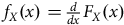 ${f_X}\left( x \right) = {d \over {dx}}{F_X}\left( x \right)$
is the density function of random variable X. Because
${f_X}\left( x \right) = {d \over {dx}}{F_X}\left( x \right)$
is the density function of random variable X. Because ${f_X}\left( x \right) = {d \over {dx}}\left( {1 - S\left( x \right)} \right) = - S'\left( x \right)$
,
${f_X}\left( x \right) = {d \over {dx}}\left( {1 - S\left( x \right)} \right) = - S'\left( x \right)$
,
 $$\mu \left( x \right) = {{{f_X}\left( x \right)} \over {S\left( x \right)}} = - {{S{\rm{'}}\left( x \right)} \over {S\left( x \right)}} = - {d \over {dx}}{\rm{ln}}S\left( x \right).$$
From the above, the probability of survival from age x to age $x + t$
, for example,
$x + t$
, for example, ${S_x}\left( t \right)$
, is given by:
${S_x}\left( t \right)$
, is given by:
 $${S_x}\left( t \right) = {\rm{exp}}\left( { - \mathop \int \nolimits_x^{x + t} \mu \left( y \right)dy} \right),$$
and so, the probability of death from age x to $x + t$
is
$x + t$
is ${P_x}\left( t \right) = 1 - {S_x}\left( t \right)$
.
${P_x}\left( t \right) = 1 - {S_x}\left( t \right)$
.
For a Cox proportional hazards model, the instantaneous probability of the event occurring is termed the “hazard rate”. Therefore when the event of interest is death, the hazard rate is equivalent to the force of mortality. The hazard rate at time t for an individual with the input information defined in vector z is denoted by $\lambda \left( {t,z} \right)$
. For a Cox proportional hazards model, the hazard rate is calculated as:
$\lambda \left( {t,z} \right)$
. For a Cox proportional hazards model, the hazard rate is calculated as:
 $$\lambda \left( {t,z} \right) = {\lambda _0}\left( t \right) \cdot {\rm{exp}}\left( {\mathop \sum \limits_{i = 0}^m {\beta _i}{z_i}} \right),$$
where ${\lambda _0}\left( t \right)$
is the baseline hazard rate and
${\lambda _0}\left( t \right)$
is the baseline hazard rate and ${\beta _i}$
are Cox model coefficients.
${\beta _i}$
are Cox model coefficients.
For each input information i within vector z there is a corresponding ${\beta _i}$
coefficient which adjusts the baseline hazard rate. The input information represents the risk factors affecting the hazard rate. Therefore, if
${\beta _i}$
coefficient which adjusts the baseline hazard rate. The input information represents the risk factors affecting the hazard rate. Therefore, if ${\beta _i} \gt 0$
the input information i (or risk factor i) increases the hazard rate and
${\beta _i} \gt 0$
the input information i (or risk factor i) increases the hazard rate and ${\beta _i} \lt 0$
decreases the hazard rate. The absolute value
${\beta _i} \lt 0$
decreases the hazard rate. The absolute value $\left| {{\beta _i}} \right|$
therefore measures the significance of risk factor i.
$\left| {{\beta _i}} \right|$
therefore measures the significance of risk factor i.
In this application of the model:
-
•
${z_0}$
is set to be the non-negative function of age. -
•
${z_i}$
, where i is length of time since diagnosis, is also set to be the non-negative function of time. -
• all other
${z_i}$
are equal to either 0 or 1, as an indicator of whether the risk factor i is present (
${z_i} = 1$
) or absent (
${z_i} = 0$
).


Given the above, (1) simplifies toFootnote 9 :
 $$\lambda \left( {t,z} \right) = {\lambda _0}\left( t \right){e^{{\beta _0}{z_0}}} \cdot {\rm{exp}}\left( {\mathop \sum \limits_{i = 1}^m {\beta _i}{z_i}} \right) = {\lambda _0}\left( t \right){e^{{\beta _0}{z_0}}} \cdot {\rm{exp}}\left( {\mathop \sum \limits_{i \in I} {\beta _i}} \right) = {\lambda _0}\left( t \right){e^{{\beta _0}{z_0}}}\mathop \prod \limits_{i \in I} {k_i},$$
where I is the set of indices i such that ${z_i} = 1$
and
${z_i} = 1$
and ${k_i} = e_i^\beta $
.
${k_i} = e_i^\beta $
.
The model provides estimates that are used to alter the overall hazard rate based on an individual’s input information. For any input information (risk factor) $i = 1, \ldots ,m$
, a change in the value of
$i = 1, \ldots ,m$
, a change in the value of ${z_i}$
from 0 to 1 alters the hazard rate
${z_i}$
from 0 to 1 alters the hazard rate $\lambda \left( {t,z} \right)$
by a factor specific to that risk factor, for example,
$\lambda \left( {t,z} \right)$
by a factor specific to that risk factor, for example, ${k_{i}}$
. If there is a change to more than one risk factor, say both
${k_{i}}$
. If there is a change to more than one risk factor, say both ${z_i}$
and
${z_i}$
and ${z_j}$
from
${z_j}$
from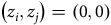 $\left( {{z_i},{z_j}} \right) = \left( {0,0} \right)$
to
$\left( {{z_i},{z_j}} \right) = \left( {0,0} \right)$
to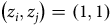 $\left( {{z_i},{z_j}} \right) = \left( {1,1} \right)$
, then this alters the hazard rate
$\left( {{z_i},{z_j}} \right) = \left( {1,1} \right)$
, then this alters the hazard rate $\lambda \left( {t,z} \right)$
by a factor
$\lambda \left( {t,z} \right)$
by a factor ${k_i}{k_j}$
. This implies that the factors i and j are acting independently. This is a key underlying assumption of the Cox proportional hazards model.
${k_i}{k_j}$
. This implies that the factors i and j are acting independently. This is a key underlying assumption of the Cox proportional hazards model.
For example, where factors i and j indicate the presence or absence of certain diseases then the model provides coefficients to alter the force of mortality based on the disease states. For example, if an individual is diabetic (D) this alters the hazard rate by a factor of ${k_D}$
; and if the individual also has hypertension (H) this alters it by
${k_D}$
; and if the individual also has hypertension (H) this alters it by ${k_H}$
. That is, an individual with both diabetes and hypertension has a hazard rate altered by a factor
${k_H}$
. That is, an individual with both diabetes and hypertension has a hazard rate altered by a factor ${k_D}{k_H}$
. It is important to note that this way of modelling is simplistic and ignores the known dynamic of a “combination of risk factors effect”. For example, hypertension may increase the probability of death to a greater extent for diabetic individuals than for non-diabetic individuals (Bell, Reference Bell2008). So far in this model description, this has not been allowed for as the model is solving the coefficient independently.
${k_D}{k_H}$
. It is important to note that this way of modelling is simplistic and ignores the known dynamic of a “combination of risk factors effect”. For example, hypertension may increase the probability of death to a greater extent for diabetic individuals than for non-diabetic individuals (Bell, Reference Bell2008). So far in this model description, this has not been allowed for as the model is solving the coefficient independently.
To take account of such combination effects, the model must solve these factors independently and then also in combination. This requires the introduction of new risk factors to represent any pair of risk factors i and j. This new risk factor indexed as ij is such that ${z_{ij}} = 1$
if an individual has both risk factors, for example, if
${z_{ij}} = 1$
if an individual has both risk factors, for example, if ${z_i} = {z_j} = 1$
; otherwise
${z_i} = {z_j} = 1$
; otherwise ${z_{ij}} = 0$
. Continuing the example for an individual with both diabetes and hypertension, the input information is therefore
${z_{ij}} = 0$
. Continuing the example for an individual with both diabetes and hypertension, the input information is therefore ${z_D} = 1$
,
${z_D} = 1$
, ${z_H} = 1$
and now,
${z_H} = 1$
and now, ${z_{DH}} = 1$
. Then, for an individual with only these two risk factors, the hazard rate formula (2) becomes:
${z_{DH}} = 1$
. Then, for an individual with only these two risk factors, the hazard rate formula (2) becomes:
 $$\lambda \left( {t,z} \right) = {\lambda _0}\left( t \right){e^{{\beta _0}{z_0}}}{k_D}{k_H}{k_{DH}}.$$
The interpretation of ${k_{DH}}$
is that it is the coefficient that accounts for the mortality risk arising from the combination of diabetes and hypertension that remains after accounting for diabetes and hypertension individually. Therefore, the factor
${k_{DH}}$
is that it is the coefficient that accounts for the mortality risk arising from the combination of diabetes and hypertension that remains after accounting for diabetes and hypertension individually. Therefore, the factor ${k_D}$
represents the alteration to baseline hazard rate for diabetes,
${k_D}$
represents the alteration to baseline hazard rate for diabetes, ${k_H}$
for hypertension and
${k_H}$
for hypertension and ${k_{DH}}$
for the alteration when both are present.
${k_{DH}}$
for the alteration when both are present.
It should be noted that the model does not account for which condition pre-dates the other, which may epidemiologically cause a variation in the force of mortality. For instance, the development of hypertension prior to diabetes may have different clinical implications than the reverse order. However, for the purpose of this research objective of mimicking the information available at the time of underwriting, this simplification is considered appropriate.
In the underwriting context, risk assessment is typically based on a snapshot of available health information at the time of application, without access to detailed longitudinal records or the precise sequence of diagnoses. Therefore, modelling co-morbid conditions as coexisting covariates, rather than in a temporally ordered fashion, aligns with the real-world data structure and decision-making process used by insurers.
Moreover, many of the granular subgroups defined by disease order (e.g., diabetes preceding hypertension versus hypertension preceding diabetes) are relatively small and statistically underpowered, which limits the reliability and interpretability of stratified hazard estimates. Attempting to model these pathways separately could introduce instability or noise into the model, especially in population-based data sets not designed to capture such detail robustly.
6.2 Model Build
Models were built iteratively with modelling choices, detailed below with supporting rationale, made along the way. These decisions were made in conjunction with ongoing discussions between Leicester University and DSG. The objective of this working relationship was to ensure that the output was fit for purpose and for the intended audience, and hence some decisions herein may vary from medical or epidemiological research. Namely, risk factors are taken as the latest observation to the study start even if the risk factor would not remain static thereafter and there is evidence that a change in that risk factor would imply a change in the mortality risk going forward. Therefore, it is known that there will be drift between mortality risk classification groups after the study start date. However, this is considered appropriate for this research objective as it mimics the underwriting process that analyses mortality risk based only on the latest observation found in the input information accessible during the underwriting stage.
The model build was undertaken in stages, each with an objective, to reach a final model to fit. The stages are:
-
• Data partitioning.
-
• Risk factor transformation.
-
• Risk factor selection.
Each stage is now described in separate subsections.
6.2.1 Data Partitioning
Sex at birth is an important factor in understanding of mortality risk (Zarulli et al., Reference Zarulli, Kashnitsky and Vaupel2021). Indeed, many risk factors including the age shape of mortality risk vary by sex (Wu et al., Reference Wu, Niubo, Daskalopoulou, Moreno-Agostino, Stefler, Bobak, Oram, Prince and Prina2021). To build more accurate models, the data set is divided by sex and the model is fitted for males and females separately. This approach offers several advantages. Stratification allows the model to capture sex-specific hazard functions and avoids the assumption of proportionality across sexes, which may be violated if key risk factors behave differently for men and women. It also enhances interpretability by enabling the direct comparison of risk profiles within each sex group, aligning with clinical evidence that diabetes presents distinct risk trajectories in males and females (Kautzky-Willer et al., Reference Kautzky-Willer, Harreiter and Pacini2016).
6.2.2 Risk Factor Transformation
The following risk factors are modelled to test the statistical significance of the factor on the mortality rate. A summary of risk factor transformation is summarised in Table 70 and the mortality statistics associated with each risk factor are presented in Table 71.
For ordered clinical variables such as BMI, BP, cholesterol, IMD and HbA1c, we use cumulative binary indicators rather than mutually exclusive categories. Under this encoding, an individual who exceeds a higher threshold also satisfies the lower thresholds. We adopted this approach because it mirrors the way underwriting rules are typically applied, preserves the ordinal structure of the risk factor and allows the model to capture the incremental effect of crossing successively more severe thresholds. We preferred this to a purely categorical encoding because the cumulative form provides a more direct interpretation of threshold effects while remaining transparent for actuarial use.
6.2.2.1 Age
Age is calculated as the number of whole years at the study start and assigned the risk factor ${z_0}$
in the model. This approach uses exact single-year age rather than broader age bands. This reflects standard practice in life insurance and actuarial modelling, where mortality assumptions are typically constructed on a per-year-of-age basis.
${z_0}$
in the model. This approach uses exact single-year age rather than broader age bands. This reflects standard practice in life insurance and actuarial modelling, where mortality assumptions are typically constructed on a per-year-of-age basis.
Using single-year age allows for more granular modelling of the age-related variation in mortality, which is known to change markedly even across adjacent years, particularly at older ages. Given the size and richness of the data set, there is sufficient statistical power to estimate risk at this fine level of resolution without the need to aggregate into coarser categories. This avoids potential loss of information and smoothing over important inflection points in the age–mortality relationship that could influence model accuracy and underwriting decisions. Moreover, insurers routinely rely on single-age mortality tables (NLT), and using a consistent age definition enhances the interpretability and practical relevance of the model outputs for actuarial and underwriting audiences.
In the model, the hazard rate (e.g., force of mortality) depends on age as:
 $$\lambda \left( {t,z} \right)\sim {e^{{\beta _0}{z_0}}},$$
where ${z_0}$
is a function of age. To determine
${z_0}$
is a function of age. To determine ${z_0}$
, the force of mortality as it varies with age must be assessed. For example, the force of mortality by age for males is presented in Figure 11. It can be seen that the force of mortality is almost linear in logarithmic coordinates. This suggests that
${z_0}$
, the force of mortality as it varies with age must be assessed. For example, the force of mortality by age for males is presented in Figure 11. It can be seen that the force of mortality is almost linear in logarithmic coordinates. This suggests that ${z_0} = $
age is already a reasonable model.
${z_0} = $
age is already a reasonable model.
However, the fit to data can be improved by assuming that ${z_0}$
is a piecewise-linear function of age. For example, the manual splitting of age interval [17–100] into three intervals of [17–27], [28–73] and [74–100] significantly improves the fit to data – see Figure 12. In order to identify intervals with the best accuracy automatic segmentation is used. The results of this segmentation are presented in Table 72, Figure 13 and Figure 14. Applying the Elbow rule to Figure 13 suggests that only 2 segments should be used. That is,
${z_0}$
is a piecewise-linear function of age. For example, the manual splitting of age interval [17–100] into three intervals of [17–27], [28–73] and [74–100] significantly improves the fit to data – see Figure 12. In order to identify intervals with the best accuracy automatic segmentation is used. The results of this segmentation are presented in Table 72, Figure 13 and Figure 14. Applying the Elbow rule to Figure 13 suggests that only 2 segments should be used. That is, ${z_0}$
is given by the formula:
${z_0}$
is given by the formula:
 $${z_0} = \left\{ {\matrix{ {k \cdot \left( {{\rm{age}} - {z^{\rm{*}}}} \right) + {z^{\rm{*}}},} \hfill & {{\rm{if\;age}} \le {z^{\rm{*}}}} \hfill \cr {{\rm{age}},} \hfill & {{\rm{if\;age}} \ge {z^{\rm{*}}},} \hfill \cr } } \right.$$
where ${z^{\rm{*}}}$
and k are fitted to the partitioned data, for example, for males and females separately. As indicated in Table 72, the optimal break point
${z^{\rm{*}}}$
and k are fitted to the partitioned data, for example, for males and females separately. As indicated in Table 72, the optimal break point ${z^{\rm{*}}}$
is 50 for males and 65 for females. The optimal value of k is
${z^{\rm{*}}}$
is 50 for males and 65 for females. The optimal value of k is $0.6510$
for males and
$0.6510$
for males and $0.7335$
for females.
$0.7335$
for females.
6.2.2.2 Body Mass Index (BMI)
The latest observation of the BMI measurement at the study start is transformed into covariates to improve model simplicity. The ranges employed are in line with those adopted by the NHS (NHS, 2023b). However, the groupings are altered to improve model accuracy: specifically, the obese range was subdivided into the 3 classes shown below, as it significantly improved model accuracy. The following risk factor transformation is introduced:
-
• Underweight:
${z_{b1}} = 1$
if BMI
$ \lt 18.5$
, and
${z_{b1}} = 0$
otherwise. -
• Overweight:
${z_{b2}} = 1$
if BMI
$ \geq\!25.0$
, and
${z_{b2}} = 0$
otherwise. -
• Obese Class 1:
${z_{b3}} = 1$
if BMI
$ \geq \!30.0$
, and
${z_{b3}} = 0$
otherwise. -
• Obese Class 2:
${z_{b4}} = 1$
if BMI
$ \geq 35.0$
, and
${z_{b4}} = 0$
otherwise. -
• Obese Class 3:
${z_{b5}} = 1$
if BMI
$ \geq 40.0$
, and
${z_{b5}} = 0$
otherwise.


For example, an individual with BMI 32.5 has a BMI which is both $ \geq 25.0$
and
$ \geq 25.0$
and $ \geq 30.0$
and so is described by a vector
$ \geq 30.0$
and so is described by a vector $\left( {{z_{b1}},{z_{b2}},{z_{b3}},{z_{b4}},{z_{b5}}} \right) = \left( {0,1,1,0,0} \right)$
. Therefore, coordinates are not independent as, for example, if
$\left( {{z_{b1}},{z_{b2}},{z_{b3}},{z_{b4}},{z_{b5}}} \right) = \left( {0,1,1,0,0} \right)$
. Therefore, coordinates are not independent as, for example, if ${z_{b3}} = 1$
then
${z_{b3}} = 1$
then ${z_{b2}} = 1$
.
${z_{b2}} = 1$
.
This structure reflects a cumulative threshold-based encoding that mirrors the way underwriters and actuaries typically think about BMI risk categories – each level of obesity builds on the previous. This encoding captures the escalating nature of risk associated with higher BMI thresholds, which is especially useful in underwriting, where risk loading increases progressively across weight categories.
6.2.2.3 Blood Pressure (BP)
Measurements for systolic blood pressure (SBP) and diastolic blood pressure (DBP) are used at the latest observation as at study start. The risk factor transformation introduced is shown below and is considered in line with NHS ranges used (NHS, 2023a):
-
• Low blood pressure:
${z_{p1}} = 1$
if either SBP
$ \le 90$
or DBP
$ \le 60$
. Otherwise
${z_{p1}} = 0$
. -
• Pre-hypertension:
${z_{p2}} = 1$
if either SBP
$ \geq 120$
or DBP
$ \geq 80$
. Otherwise
${z_{p2}} = 0$
. -
• High BP (Stage 1):
${z_{p3}} = 1$
if either SBP
$ \geq 140$
or DBP
$ \geq 90$
. Otherwise
${z_{p3}} = 0$
. -
• High BP (Stage 2):
${z_{p4}} = 1$
if either SBP
$ \geq 160$
or DBP
$ \geq 100$
. Otherwise
${z_{p4}} = 0$
.


In terms of insurance underwriting, BP is routinely assessed at point of application, and risk assessment typically involves identifying whether an individual exceeds particular thresholds that align with these exact categories. Many underwriting manuals apply stepwise premium loadings based on these categories, and reinsurer rating guides often treat elevated BP levels as risk multipliers, particularly in the presence of co-morbid conditions like diabetes or obesity.
6.2.2.4 Cholesterol Levels (CL)
Measurements for Cholesterol levels (CL) are used at the latest observation as at study start. The risk factor transformation introduced is shown below and is informed/based on widely used clinical guidelines (Superdrug Online Doctor, 2023):
-
• High CL:
${z_{c1}} = 1$
if CL
$ \gt 5$
mmol/L. Otherwise
${z_{c1}} = 0$
. -
• Very high CL:
${z_{c2}} = 1$
if CL
$ \gt 6.5$
mmol/L. Otherwise
${z_{c2}} = 0$
. -
• Extremely high CL:
${z_{c3}} = 1$
if CL
$ \gt 7.8$
mmol/L. Otherwise
${z_{c3}} = 0$
.


In the underwriting context, elevated cholesterol is a known risk factor and often triggers further review or a premium loading. While insurers may use more comprehensive lipid panels, TC remains a common and interpretable metric. The use of the most recent value at the time of underwriting is standard practice, as underwriters make risk assessments based on an individual’s current health status, not historical averages or trends. The cumulative structure of the indicators (e.g., someone with CL = $8.0$
mmol/L will satisfy all three conditions) reflects the increasing risk load and provides flexibility in the model to capture marginal effects across ranges.
$8.0$
mmol/L will satisfy all three conditions) reflects the increasing risk load and provides flexibility in the model to capture marginal effects across ranges.
6.2.2.5 Smoking Status
Smoking status is based on the categorisation defined at the study start. The risk factor transformation introduced is shown below and is informed by epidemiological and actuarial research demonstrating the differential mortality risks associated with current, former and never smokers (Doll et al., Reference Doll, Peto, Boreham and Sutherland2004).
-
• Ever smoked:
${z_{s1}} = 1$
if an individual ever smoked. Otherwise
${z_{s1}} = 0$
. -
• Current smoker:
${z_{s2}} = 1$
if an individual is a current smoker. Otherwise
${z_{s2}} = 0$
.


That is to say, at the study start, $\left( {{z_{s1}},{z_{s2}}} \right) = \left( {0,0} \right)$
is an individual that never smoked,
$\left( {{z_{s1}},{z_{s2}}} \right) = \left( {0,0} \right)$
is an individual that never smoked, $\left( {{z_{s1}},{z_{s2}}} \right) = \left( {1,0} \right)$
an individual who is an ex-smoker and
$\left( {{z_{s1}},{z_{s2}}} \right) = \left( {1,0} \right)$
an individual who is an ex-smoker and $\left( {{z_{s1}},{z_{s2}}} \right) = \left( {1,1} \right)$
an individual who is a smoker.
$\left( {{z_{s1}},{z_{s2}}} \right) = \left( {1,1} \right)$
an individual who is a smoker.
This approach is reasonable and aligns well with underwriting practices, where smoking status is a key and typically static data point collected at application. While smoking behaviour can change over time, underwriting generally relies on smoking status reported or verified at the point of underwriting, which is assumed to be constant for pricing and risk classification purposes.
6.2.2.6 Index of Multiple Deprivation (IMD)
The IMD is taken as at the study start. The risk factor is transformed using 4 variables set to either a value of 0 or 1.
-
•
${z_{md1}} = 1$
if IMD level is at least 3, and
${z_{md1}} = 0$
otherwise. -
•
${z_{md2}} = 1$
if IMD level is at least 5, and
${z_{md2}} = 0$
otherwise. -
•
${z_{md3}} = 1$
if IMD level is at least 7, and
${z_{md3}} = 0$
otherwise. -
•
${z_{md4}} = 1$
if IMD level is at least 9, and
${z_{md4}} = 0$
otherwise.


In other words, IMD levels 1 and 2 are coded as $\left( {0,0,0,0} \right)$
, IMD 3 and 4 as
$\left( {0,0,0,0} \right)$
, IMD 3 and 4 as $\left( {1,0,0,0} \right)$
, IMD 5 and 6 as
$\left( {1,0,0,0} \right)$
, IMD 5 and 6 as $\left( {1,1,0,0} \right)$
, IMD 7 and 8 as
$\left( {1,1,0,0} \right)$
, IMD 7 and 8 as $\left( {1,1,1,0} \right)$
and IMD 9 and 10 as
$\left( {1,1,1,0} \right)$
and IMD 9 and 10 as $\left( {1,1,1,1} \right)$
.
$\left( {1,1,1,1} \right)$
.
From an underwriting perspective, the IMD is assumed to be a static data point, reflecting the individual’s health or risk profile at the point of underwriting (i.e., study start). This is consistent with insurance risk assessment practices where data used for pricing or risk classification is typically fixed at application. Although individuals’ health status may change over time, underwriting decisions usually cannot account for such longitudinal variations. Additionally, using this binary stepwise transformation avoids potential issues with sparse data if the IMD were used as a continuous variable or in very granular categories. It also simplifies interpretation for underwriters and actuaries, who can associate specific IMD threshold levels with corresponding risk adjustments.
6.2.2.7 Diabetes Disease Status
The diabetes disease status is encoded based on diagnoses as at the start of the study. A later diagnosis is not considered relevant because this approach mimics the real-world underwriting process in insurance. In insurance underwriting, the assessment of mortality risk and premium setting is based on the information available at the time of application, which includes the individual’s current health conditions and medical history up to that date. Later developments or diagnoses occurring after the policy issue date are generally not factored into the initial risk classification, as underwriting decisions and pricing are fixed at inception. The transformation of this data item is:
-
•
${z_{D1}} = 1$
if an individual has been diagnosed with Type 1 diabetes, and
${z_{D1}} = 0$
otherwise. -
•
${z_{D2}} = 1$
if an individual has been diagnosed with Type 2 diabetes, and
${z_{D2}} = 0$
otherwise.


For example, an individual diagnosed with Type 2 diabetes in June 2010 has ${z_{D1}}$
and
${z_{D1}}$
and ${z_{D2}}$
of
${z_{D2}}$
of $\left( {0,0} \right)$
.
$\left( {0,0} \right)$
.
It is considered reasonable to model Type 1 and Type 2 diabetes separately when estimating mortality risk because these conditions differ significantly in their pathophysiology, typical age of onset, progression, complications and associated mortality patterns. Numerous epidemiological studies have demonstrated statistically significant differences in mortality risk between individuals with Type 1 and Type 2 diabetes, see, for example, Genuth et al. (Reference Genuth, Palmer and Nathan2021).
6.2.2.8 Duration since Diabetes Diagnosis
This risk factor is only considered for individuals with diabetes. For an individual with Type i diabetes, $i = 1,2$
, it measures the duration (in years) since the Type i diabetes was diagnosed. This is computed by the formula “2009 – calendar year of the diagnosis” given the study start of 01/01/2010. For example, an individual diagnosed in June 2009 with Type 2 diabetes has a duration since diagnosis of
$i = 1,2$
, it measures the duration (in years) since the Type i diabetes was diagnosed. This is computed by the formula “2009 – calendar year of the diagnosis” given the study start of 01/01/2010. For example, an individual diagnosed in June 2009 with Type 2 diabetes has a duration since diagnosis of $2009 - 2009 = 0$
. Duration therefore increases in whole numbers from 0.
$2009 - 2009 = 0$
. Duration therefore increases in whole numbers from 0.
Including duration since diagnosis as a risk factor is reasonable and important for mortality risk modelling because the length of time an individual has lived with diabetes is strongly associated with the progression of complications and overall mortality risk (Wright et al., Reference Wright, Suarez-Ortegon, Read, Kontopantelis, Buchan, Emsley, Sattar, Ashcroft, Wild and Rutter2020).
From an underwriting perspective, while duration since diagnosis may not always be explicitly recorded, it is often estimated or indirectly assessed through medical history or reported diagnosis dates. Incorporating this information aligns with underwriting practices that seek to assess not only the presence of a condition but also its chronicity and severity, which influences risk classification and pricing decisions. It is assumed that duration as a static variable at study start is consistent with underwriting timelines, where risk is assessed based on information available at application. This approach balances model complexity and practical utility, providing a meaningful metric to enhance mortality risk prediction for individuals with diabetes.
6.2.2.9 Blood Glucose (sugar) Level (HbA1c)
Measurements for blood glucose (sugar) level (HbA1c) are used at the latest observation as at study start. The risk factor is transformed using the ranges defined by guidelines such as those from the American Diabetes Association (ADA) and the World Health Organization (WHO):
-
• Pre-diabetes:
${z_{h1}} = 1$
if HbA1c
$ \geq 6.0{\rm{\% }}$
. Otherwise
${z_{h1}} = 0$
. -
• Diabetes:
${z_{h2}} = 1$
if HbA1c
$ \geq 6.5{\rm{\% }}$
. Otherwise
${z_{h2}} = 0$
. -
• Diabetes high:
${z_{h3}} = 1$
if HbA1c
$ \geq 7.5{\rm{\% }}$
. Otherwise
${z_{h3}} = 0$
. -
• Diabetes very high:
${z_{h4}} = 1$
if HbA1c
$ \geq 9.0{\rm{\% }}$
. Otherwise
${z_{h4}} = 0$
.


These variables define certain HbA1c ranges. For example, an HbA1c $ \lt 6.0\% $
is defined by
$ \lt 6.0\% $
is defined by $\left( {0,0,0,0} \right)$
, an HbA1c between
$\left( {0,0,0,0} \right)$
, an HbA1c between $6.0$
and
$6.0$
and $6.5$
by
$6.5$
by $\left( {1,0,0,0} \right)$
, an HbA1c between
$\left( {1,0,0,0} \right)$
, an HbA1c between $6.5$
and
$6.5$
and $7.5$
as
$7.5$
as $\left( {1,1,0,0} \right)$
, and so on.
$\left( {1,1,0,0} \right)$
, and so on.
From an underwriting perspective, HbA1c is a key biomarker routinely assessed and recorded in medical underwriting questionnaires or clinical tests. Using the latest available value at study start reflects standard underwriting practice, where the most recent medical data available at application is used for risk classification. Although HbA1c can fluctuate, the latest measurement provides a practical snapshot of glycemic control and risk status. The cumulative binary coding captures clinically meaningful cutoffs while maintaining simplicity and interpretability for underwriting decisions. It balances granularity with data availability and aligns well with mortality risk modelling objectives focused on diabetes-related risk stratification.
6.2.2.10 Disease Status
For each of the diseases listed in Section 4.1, ${z_i}$
is set to 1 if disease i has ever been diagnosed at the study start and
${z_i}$
is set to 1 if disease i has ever been diagnosed at the study start and ${z_i} = 0$
otherwise. Diagnoses do occur during the study period. To keep vector z constant for each individual, the following strategy is introduced:
${z_i} = 0$
otherwise. Diagnoses do occur during the study period. To keep vector z constant for each individual, the following strategy is introduced:
-
• If disease i has never been diagnosed then
${z_i} = 0$
. -
• If disease i has been diagnosed before the study start, then
${z_i} = 1$
. -
• If disease i has been diagnosed x years after the study start, then we split the record into two pseudo-individual records: one with
${z_i} = 0$
for x years and one with
${z_i} = 1$
for the remaining
$10 - x$
years.


6.2.2.11 Pairwise Interaction of Risk Factors
For each pair $\left( {i,j} \right)$
of risk factors discussed above, a new risk factor is introduced
$\left( {i,j} \right)$
of risk factors discussed above, a new risk factor is introduced ${z_{ij}} = {z_i}{z_j}$
. For example, if each
${z_{ij}} = {z_i}{z_j}$
. For example, if each ${z_i}$
and
${z_i}$
and ${z_j}$
takes values in
${z_j}$
takes values in $\left\{ {0,1} \right\}$
, then
$\left\{ {0,1} \right\}$
, then ${z_{ij}} \in \left\{ {0,1} \right\}$
, and
${z_{ij}} \in \left\{ {0,1} \right\}$
, and ${z_{ij}} = 1$
if and only if
${z_{ij}} = 1$
if and only if ${z_i} = {z_j} = 1$
.
${z_i} = {z_j} = 1$
.
Higher order interactions are not considered because on balance the working group prioritised having coefficient value outputs which could be easily interpreted.
6.2.3 Risk Factor Selection Process
An iterative model fitting process was employed; before fitting a final model with all risk factors and meaningful pairwise interactions, we built some simplified models with only some of the attributes included. In all models, the coefficients ${\beta _i}$
can be computed by maximum likelihood method. An important feature of the Cox proportional hazards model is that the baseline hazard rate
${\beta _i}$
can be computed by maximum likelihood method. An important feature of the Cox proportional hazards model is that the baseline hazard rate ${\lambda _0}\left( t \right)$
is not needed to compute
${\lambda _0}\left( t \right)$
is not needed to compute ${\beta _i}$
, hence they can be computed first. This is used here to allow for risk factor selection.
${\beta _i}$
, hence they can be computed first. This is used here to allow for risk factor selection.
-
• Model A: a model without data partitioning and with no diseases and no interaction attributes. All other risk factors described in Section 6.2.2 are included. Risk factor selection is then considered via backward and forward feature selection (FFS) process. In Model A, the data is not partitioned by sex and this ensures the same set of risk factors are included for males and females. The objective of model A aligns with our desire to understand the influence of “industry standard” underwriting risk factors (such as age, gender, BMI, etc.) on the mortality risk of individuals from GS. Another objective is to have a simple but reasonable model as a benchmark with which the more complicated models can be compared.
-
• Model B: a model with data partitioning, allowing for disease status independently but not in combination (all risk factors in Section 6.2.2 except pairwise disease interactions). As a minimum, the model must include “industry standard” underwriting risk factor classifications. These risk factors are protected and are not subject to the selection process. Other risk factors (diseases) are selected via backward and FFS processes. The objective of model B is to understand the influence of various co-morbidities on the mortality risk of individuals from GS as stand-alone factors, without taking into account interaction. Another objective is to have this model as a benchmark with which our main model (with interactions) can be compared.
The objective of including pairwise interactions of attributes in the model is to capture non-additive effects and synergistic relationships between risk factors – especially among co-morbidities – that may jointly influence mortality risk in ways not apparent when considered in isolation. Certain combinations of risk factors (e.g., cardiovascular disease and high BMI) may result in elevated or diminished hazard beyond what would be expected from their individual effects.
6.2.3.1 Risk Factor Selection: Backward and Forward Feature Selection
The objective of this step is to build Model A by selecting meaningful non-disease and non-interaction risk factors, independent of sex, that have significant influence on the mortality of individuals with diabetes.
Model A includes all risk factors listed in Section 6.2.2, apart from the disease status and interaction risk factors. As the data is not partitioned, a risk factor of sex is introduced to account for variation. The model is fit on the GS data. The resulting coefficients are presented in Table 76, alongside the standard errors (SE) and p-values, where the p-value measures the significance of the risk factor and a higher p-value indicates a lower significance. Risk factors with a p-value greater than 0.01 are considered insignificant. We use a 1% threshold rather than the more conventional 5% because the data set is very large, so a 5% cutoff would retain many effects that are statistically detectable but too weak to be useful in a parsimonious underwriting model. The stricter threshold therefore helps reduce over-fitting and focuses the model on the most robust signals. Table 76 therefore contains 7 insignificant attributes. Risk factor selection can be reviewed by starting with the full list of 20 risk factors (as above) and removing those considered insignificant via the backward feature selection (BFS) process. The process of BFS (or dimensionality reduction) removes variables with the greatest p-values one-by-one until there is at least one statistically insignificant variable. The results are presented in Table 77. The model resulting from this process is presented in the right side of Table 76. Assuming that the baseline hazard rate is given by the exponential model (8) described below, the computed parameters are:
-
•
$a = 0.0552$
,
$b = - 12.3610$
for the full model (before exclusion of insignificant risk factors). -
•
$a = 0.0553$
,
$b = - 12.3236$
for the reduced model (after exclusion of insignificant risk factors).




Correlation matrix between risk factors of the full model is presented in Table 78. The removed risk factors are strongly correlated with the remaining risk factors.
Table 76 shows some risk factors with negative coefficients, that is, the presence of the corresponding risk factor decreases the baseline force of mortality. Most risk factors with negative coefficients in the model also exhibit a moderate to strong positive correlation with age. This suggests that their apparent protective effect may be confounded by age: these factors become more common in older individuals, but age itself is already a strong predictor of increased mortality. Thus, when age is controlled for in the model, these variables may appear to lower risk simply because they are positively associated with age, not necessarily because they are truly protective. However, the variable Cl3 is an exception. Despite having a negligible correlation with age ( $0.032$
), it retains a significant negative coefficient. This finding aligns with the “Cholesterol Paradox” often observed in observational studies of chronic diseases (Wang et al., Reference Wang, Chang, Wei, Liu, Tzeng and Chiu2023). In this context, the inverse association between cholesterol and mortality is typically attributed to reverse causality, where low CLs serve as a marker for underlying frailty, malnutrition, or chronic inflammation; rather than higher CLs conferring a direct biological benefit.
$0.032$
), it retains a significant negative coefficient. This finding aligns with the “Cholesterol Paradox” often observed in observational studies of chronic diseases (Wang et al., Reference Wang, Chang, Wei, Liu, Tzeng and Chiu2023). In this context, the inverse association between cholesterol and mortality is typically attributed to reverse causality, where low CLs serve as a marker for underlying frailty, malnutrition, or chronic inflammation; rather than higher CLs conferring a direct biological benefit.
To understand the meaning of a negative coefficient (see Table 76), a direct estimation of the force of mortality for age bands is calculated using the GS data (we do not have enough data for mortality estimation for each year separately). Results are presented in Tables 79–84. As you can see, in all cases negative coefficients were explained by the supporting data. In other words, the observed negative dependence is really present in the data, it is not an artefact of the model.
Alternatively, FFS can be employed; starting with one attribute (e.g., age), and adding the next “most significant” (measured by p-value) risk factor one-by-one, until there are no more significant risk factors. The results are presented in Tables 85 and 86.
The models resulting from BFS and FFS are both the same, which provides confidence in the robustness and stability of the selected set of risk factors. This convergence suggests that the final feature set is not overly sensitive to the choice of selection method and likely reflects genuinely important predictors within the data.
6.2.3.2 Risk Factor Selection: Industry Standard Risk Classification
In Model B and the final output models, attributes describing age, IMD, BMI, BP, smoker status and CL are classified as “industry standard” and therefore must be included in the model, irrespective of their significance. There are other risk factors commonly used in the industry that are not included in our models. For example, family medical history, occupation and physical activity levels, are often considered in traditional underwriting are omitted due to data availability constraints.
The exclusion of these factors presents both benefits and limitations. On the one hand, the streamlined model may be easier to implement and explain, reducing complexity and potential biases introduced by subjective or self-reported data. On the other hand, it may compromise predictive accuracy, especially for edge cases where lifestyle or family medical history plays a crucial role. It is not possible, at this time, to test the impact, however, as the data is not recorded within the available data.
6.2.3.3 Risk Factor Selection: Disease Significance Considered by Sex
Model B partitions the data by sex and considers all risk factors from Section 6.2.2, excluding only the disease pairwise interactions.
As explained in Section 6.2.2, diseases are diagnosed during the study period, and, to keep attribute vector z constant for each individual, we split the records of such individuals into two pseudo-individual records: one without this disease from the beginning of the study to the date of diagnosis, and another one with this disease from the date of diagnosis. In case of several different diagnoses, an individual record can be split into more than two records. After such splitting of general sample linked to ONS, we obtained a data set with 157,143 records.
Table 87 presents the resulting Cox coefficients. There are 12 negative coefficients. A comparison of Cox coefficients for models A and B (e.g., with and without diseases) is presented in Table 88. A notable change is that a cholesterol observation in the “high” range (i.e., Cl) has a significant negative coefficient value in Model A (without disease status) to a significant positive coefficient value in Model B (with diseases). This suggests that the Cholesterol paradox is diminished somewhat after allowing for disease.
Risk factors with a p-value greater than 1% can be considered “insignificant” but may still be included where these are considered “industry standard risk classification”. The 1% cutoff is used deliberately here because, with a data set of this size, a 5% threshold would retain many effects that are statistically detectable but too small to be useful in a practical underwriting model. With the objective of minimising “over-fit” of the data, other insignificant attributes can be removed one-by-one until all the remaining attributes are significant. This process is undertaken on the partitioned data, for example, for males and females separately. The Cox coefficients for the models fit to the partitioned data are presented in Tables 89 and 90, for males and females respectively. In terms of statistical significance, some notable differences emerge due to sex partitioning and disease status. Several covariates demonstrate significance in one sex but not the other, highlighting underlying biological and epidemiological variations. Specifically, two male-specific diseases were found to be statistically significant for males but not for females. Conversely, seven female-specific diseases are significant only in the female cohort. The observed variation underscores the reasonableness and necessity of sex-specific modelling approaches. Sex-based biological differences (e.g., hormonal influences, genetic expression) and social determinants (e.g., healthcare access and behaviour) contribute to distinct patterns of morbidity and mortality. Incorporating these nuances into survival models enhances both statistical robustness and appropriate understanding of risk.
6.2.3.4 Risk Factor Selection: Pairwise Interactions Considered by Sex
To form models with interactions we consider all individual attributes and all possible pairs of attributes. Initially, we have 59 individual attributes and $59\cdot58/2 = 1,711$
pairs. However, some “interactions” are duplicates,Footnote
10
and were therefore removed. We also removed interactions for which there are less than 100 individuals in the data set. After this, 1,616 attributes remain for males and 1,573 for females.
$59\cdot58/2 = 1,711$
pairs. However, some “interactions” are duplicates,Footnote
10
and were therefore removed. We also removed interactions for which there are less than 100 individuals in the data set. After this, 1,616 attributes remain for males and 1,573 for females.
Fitting Cox coefficients for this number of attributes is not possible in one go due to insufficient memory, even on a supercomputer. Therefore, the following procedure is employed:
-
(i) Start with “industry standard risk factors”, that is, attributes describing age, IMD, BMI, BP, smoker status and CL.
-
(ii) Add one of several other attributes (e.g., diseases attributes or interaction attributes).
-
(iii) Compute Cox coefficients of the resulting model.
-
(iv) Remove insignificant attributes, that is, with p-value greater than 0.01. If an “industry standard risk factor” attribute is insignificant, it can be removed unless it is the last attribute in the corresponding group. That is, the age attribute is protected and cannot be removed. Out of 4 IMD attributes, at least one should stay, and so on.
-
(v) Go to step (ii) and repeat the process, until all attributes are considered.
The result of the procedure described depends on the order in which we add the attributes in step (ii). To make the procedure reproducible, we must fix the order. To establish the order in which the attributes are added in step (ii), we have used Lasso (least absolute shrinkage and selection operator) method. This method is based on minimising sum-of-squares error. It has been originally developed for regression analysis and has been adapted for the Cox model (Tibshirani, Reference Tibshirani1997). It has been implemented in the glmnet package for R. The main advantage of this method is that it works much faster than the procedure (i)–(v) above and produces a ranking of the attributes. The disadvantage is that the resulting ranking is inaccurate (some significant interactions are ranked low by Lasso and vice versa) and therefore cannot be used alone to build the final model. However, it can be used to form the initial order of attributes before applying the main procedure (i)–(v).
For female and male models, the resulting list of attributes and their Cox coefficients and p-values are presented in Tables 93 and 94, respectively.
6.3 Model Fitting
6.3.1 Computing Coefficients Values
The coefficients ${\beta _i}$
in (1) can be computed by maximum likelihood method. We record the order in which we have observed deaths, write down the likelihood function that individuals die in this particular order and then find the parameters that maximise the likelihood.
${\beta _i}$
in (1) can be computed by maximum likelihood method. We record the order in which we have observed deaths, write down the likelihood function that individuals die in this particular order and then find the parameters that maximise the likelihood.
6.3.2 Computing the Baseline Hazard Rate: Time Homogeneous and Exponential Models
After computing the Cox coefficients, the next step is computing the base rate ${\lambda _0}\left( t \right)$
. Time is measured in years and therefore the study period corresponds to the interval
${\lambda _0}\left( t \right)$
. Time is measured in years and therefore the study period corresponds to the interval $t \in \left[ {2010,2020} \right)$
. We first assume that
$t \in \left[ {2010,2020} \right)$
. We first assume that $\lambda \left( t \right)$
is a piecewise constant function, that is,
$\lambda \left( t \right)$
is a piecewise constant function, that is, $\lambda \left( t \right) = {\lambda _j}$
is a constant during year j, where
$\lambda \left( t \right) = {\lambda _j}$
is a constant during year j, where $j = 2010,2011, \ldots ,2019$
. We then estimate each
$j = 2010,2011, \ldots ,2019$
. We then estimate each ${\lambda _j}$
separately from the data.
${\lambda _j}$
separately from the data.
We next consider one year of data during a specific year j. Then $\lambda \left( t \right) = {\lambda _j}$
is a constant, and
$\lambda \left( t \right) = {\lambda _j}$
is a constant, and $\lambda \left( {t,z} \right)$
in (1) becomes
$\lambda \left( {t,z} \right)$
in (1) becomes $\lambda \left( z \right)$
, and (1) can be rewritten as:
$\lambda \left( z \right)$
, and (1) can be rewritten as:
 $$\lambda \left( z \right) = {\lambda _j} \cdot {\rm{exp}}\left( {\mathop \sum \limits_{i = 0}^m {\beta _i}{z_i}} \right) = {\lambda _j}B\left( z \right),$$
where $B\left( z \right) = {\rm{exp}}\left( {\mathop \sum \nolimits_{i = 0}^m {\beta _i}{z_i}} \right)$
.
$B\left( z \right) = {\rm{exp}}\left( {\mathop \sum \nolimits_{i = 0}^m {\beta _i}{z_i}} \right)$
.
We will estimate ${\lambda _j}$
using the method of moments. Because we need to estimate just one parameter, we can use just the first moment (the expected value). Let
${\lambda _j}$
using the method of moments. Because we need to estimate just one parameter, we can use just the first moment (the expected value). Let $A = \left( {{a_1}, \ldots ,{a_n}} \right)$
be the set of individuals that remained alive during the whole year j and let
$A = \left( {{a_1}, \ldots ,{a_n}} \right)$
be the set of individuals that remained alive during the whole year j and let $D = \left( {{d_1}, \ldots ,{d_k}} \right)$
be the set of individuals who died during the year j. Let X be the random variable indicating the number of deaths in this sample. Then, the expected number of deaths is:
$D = \left( {{d_1}, \ldots ,{d_k}} \right)$
be the set of individuals who died during the year j. Let X be the random variable indicating the number of deaths in this sample. Then, the expected number of deaths is:
 $$E\left[ X \right] = \mathop \sum \limits_{i \in A \cup D} E\left[ {{X_i}} \right],$$
where ${X_i}$
is the number of deaths for individual i, and the summation is over the whole sample
${X_i}$
is the number of deaths for individual i, and the summation is over the whole sample $A \cup D$
. As
$A \cup D$
. As ${X_i}$
can only take values 0 or 1, the formula becomes:
${X_i}$
can only take values 0 or 1, the formula becomes:
 $$E\left( {{X_i}} \right) = 0 \cdot P\left( {{X_i} = 0} \right) + 1 \cdot P\left( {{X_i} = 1} \right) = P\left( {{X_i} = 1} \right) = 1 - {\rm{exp}}\left( { - {\lambda _j}B\left( {{z_i}} \right)} \right) \approx {\lambda _j}B\left( {{z^i}} \right),$$
where ${z^i}$
is the vector of covariates for individual i, and the last approximate equality follows from the fact that
${z^i}$
is the vector of covariates for individual i, and the last approximate equality follows from the fact that $B\left( {{z^i}} \right)$
is typically small and, for small x,
$B\left( {{z^i}} \right)$
is typically small and, for small x, $1 - {\rm{exp}}\left( { - x} \right) \approx x$
. The generalised formula therefore reads as:
$1 - {\rm{exp}}\left( { - x} \right) \approx x$
. The generalised formula therefore reads as:
 $$E\left( X \right) = \mathop \sum \limits_{i \in A \cup D} E\left[ {{X_i}} \right] = \mathop \sum \limits_{i \in A \cup D} \left( {1 - {\rm{exp}}\left( { - {\lambda _j}B\left( {{z^i}} \right)} \right)} \right) \approx {\lambda _j}\mathop \sum \limits_{i \in A \cup D} B\left( {{z^i}} \right).$$
If the observed number of deaths is k, then let us find ${\lambda _j}$
from the assumption that the observed number is equal to the expected. Then:
${\lambda _j}$
from the assumption that the observed number is equal to the expected. Then:
 $${\lambda _j} \approx k{\left( {\mathop \sum \limits_{i \in A \cup D} B\left( {{z^i}} \right)} \right)^{ - 1}}.$$
In this way we can estimate ${\lambda _j}$
based on data from years
${\lambda _j}$
based on data from years $j = 2010,2011, \ldots 2019$
.
$j = 2010,2011, \ldots 2019$
.
6.3.2.1 Time-Homogeneous Model
We next consider models in which ${\lambda _0}\left( t \right)$
is a continuous function. We first consider a time-homogeneous model, which is based on the following assumption
${\lambda _0}\left( t \right)$
is a continuous function. We first consider a time-homogeneous model, which is based on the following assumption
-
• Consider two individuals A and B with the same set of attributes
${z_1}, \ldots ,{z_m}$
but different ages. Consider two different time moments
${t_1}$
and
${t_2}$
. Assume that the age of A at time
${t_1}$
is equal to the age of B at time
${t_2}$
, and this age is greater than
${z^{\rm{*}}}$
defined in (4). Then the force of mortality of A at
${t_1}$
is equal to the force of mortality of B at
${t_2}$
.


In other words, the assumption states that the probability of death depends on risk factors and current age, but not on calendar year. For example, if individual A was born in 1940 and individual B in 1945, and these individuals are otherwise identical, then the probability of death of A in 2010 (age 70) is the same as the probability of death of B in 2015 (also age 70).
From (2), the mortality rate of A at ${t_1}$
is:
${t_1}$
is:
 $${\lambda _0}\left( {{t_1}} \right){e^{{\beta _0}{z_0}\left( A \right)}} \cdot {\rm{exp}}\left( {\mathop \sum \limits_{i = 1}^m {\beta _i}{z_i}} \right),$$
while the mortality rate of B at ${t_2}$
is:
${t_2}$
is:
 $${\lambda _0}\left( {{t_2}} \right){e^{{\beta _0}{z_0}\left( B \right)}} \cdot {\rm{exp}}\left( {\mathop \sum \limits_{i = 1}^m {\beta _i}{z_i}} \right),$$
where ${z_0}\left( A \right)$
and
${z_0}\left( A \right)$
and ${z_0}\left( B \right)$
are the values of attribute
${z_0}\left( B \right)$
are the values of attribute ${z_0}$
for A and B, respectively.
${z_0}$
for A and B, respectively.
Hence, the time-homogeneity assumption implies that
 $${\lambda _0}\left( {{t_1}} \right){e^{{\beta _0}{z_0}\left( A \right)}} = {\lambda _0}\left( {{t_2}} \right){e^{{\beta _0}{z_0}\left( B \right)}}$$
or equivalently,
 $${{{\lambda _0}\left( {{t_1}} \right)} \over {{\lambda _0}\left( {{t_2}} \right)}} = {e^{{\beta _0}\left( {{z_0}\left( B \right) - {z_0}\left( A \right)} \right)}}.$$
Because the age is greater than ${z^{\rm{*}}}$
, (4) implies that
${z^{\rm{*}}}$
, (4) implies that ${z_0}\left( A \right)$
and
${z_0}\left( A \right)$
and ${z_0}\left( B \right)$
are the ages of A and B, respectively, at the start of the study. The difference in age is therefore,
${z_0}\left( B \right)$
are the ages of A and B, respectively, at the start of the study. The difference in age is therefore, ${z_0}\left( B \right) - {z_0}\left( A \right)$
. Because the age of A at time
${z_0}\left( B \right) - {z_0}\left( A \right)$
. Because the age of A at time ${t_1}$
is equal to the age of B at time
${t_1}$
is equal to the age of B at time ${t_2}$
, this implies that
${t_2}$
, this implies that
 $${z_0}\left( B \right) - {z_0}\left( A \right) = {t_1} - {t_2}.$$
Hence,
 $${{{\lambda _0}\left( {{t_1}} \right)} \over {{\lambda _0}\left( {{t_2}} \right)}} = {e^{{\beta _0}\left( {{t_1} - {t_2}} \right)}}.$$
The only function that satisfies this equality for every pair of real numbers ${t_1},{t_2}$
is the function
${t_1},{t_2}$
is the function
 $${\lambda _0}\left( t \right) = {e^{{\beta _0}t + b}}$$
for some parameter b. The constant b is then estimated by fitting (7) to the annual values ${\lambda _j}$
,
${\lambda _j}$
, $j = 2010, \ldots ,2019$
, obtained from (6).
$j = 2010, \ldots ,2019$
, obtained from (6).
6.3.2.2 Exponential Model
The only disadvantage of a time-homogeneous model is that it ignores the improvement of medicine over time. In reality, a 50-year-old individual with cancer has a higher chance to survive in 2020 than in 1970. To incorporate this effect, we can adjust the model as:
 $${\lambda _0}\left( t \right) = {e^{\left( {{\beta _0} - \varepsilon } \right)t + b}},$$
where $\varepsilon $
is the term responsible for medicine improvement. Denoting
$\varepsilon $
is the term responsible for medicine improvement. Denoting $a = {\beta _0} - \varepsilon $
, we obtain:
$a = {\beta _0} - \varepsilon $
, we obtain:
 $${\lambda _0}\left( t \right) = {e^{at + b}}.$$
Parameters a and b can then be found to best fit the data ${\lambda _j}$
,
${\lambda _j}$
, $j = 2010, \ldots ,2019$
found from (6). We will call (8) the exponential model for baseline hazard rate.
$j = 2010, \ldots ,2019$
found from (6). We will call (8) the exponential model for baseline hazard rate.
Obviously, we may also shift the numbering of years, so that t is the time (measured in years) from study start. Then t ranges in $\left[ {0,10} \right)$
for the study period.
$\left[ {0,10} \right)$
for the study period.
In both the homogeneous model (7) and exponential model (8) the hazard rate (1) has the form:
 $$\lambda \left( t \right) = {A_z}{e^{\gamma t}},$$
where ${A_z}$
is some constant that depends on vector z of attributes and
${A_z}$
is some constant that depends on vector z of attributes and $\gamma $
is equal to
$\gamma $
is equal to ${\beta _0}$
and a in homogeneous and exponential models, respectively.
${\beta _0}$
and a in homogeneous and exponential models, respectively.
Then the probability $S\left( {{t_0},{t_1}} \right)$
to survive from time
$S\left( {{t_0},{t_1}} \right)$
to survive from time ${t_0}$
to time
${t_0}$
to time ${t_1}$
is:
${t_1}$
is:
 $$S\left( {{t_0},{t_1}} \right) = {\rm{exp}}\left( { - \mathop \int \nolimits_{{t_0}}^{{t_1}} \lambda \left( t \right)dt} \right) = {\rm{exp}}\left( { - \mathop \int \nolimits_{{t_0}}^{{t_1}} {A_z}{e^{\gamma t}}dt} \right) = {\rm{exp}}\left( { - {{{A_z}} \over \gamma }\left( {{e^{\gamma {t_1}}} - {e^{\gamma {t_0}}}} \right)} \right).$$
Once we compute the survival probability, we can easily compute any other quantities of interest. For example, the expected survival time at time ${t_0}$
is given by:
${t_0}$
is given by:
 $$E\left( {{t_0}} \right) = \mathop \int \nolimits_0^\infty S\left( {{t_0},{t_0} + t} \right){\rm{\;}}dt = \mathop \int \nolimits_0^\infty {\rm{exp}}\left( { - {{{A_z}{e^{\gamma {t_0}}}} \over \gamma }\left( {{e^{\gamma t}} - 1} \right)} \right)dt.$$
Having fit the model, the survival or death probability for a given set of inputs can be found using formula (9). From this, an estimate of life expectancy can be found using formula (10).
6.3.3 Models Fit by Sample
The process of building the final models with all attributes and interactions is undertaken upon the different data samples to ensure that the models capture population-specific risk dynamics and allow for accurate estimation of mortality across distinct subgroups. Stratifying the data in this way enables the identification of both shared and unique predictors of mortality within and between groups, accounting for differences in sex and disease pathology. Namely, the models are fitted to the following:
-
• Mortality models for general population, for males and females separately.
-
• Mortality models for individuals with Type 1 diabetes, for males and females separately.
-
• Mortality models for individuals with Type 2 diabetes, for males and females separately.
Therefore, a time-homogeneous and exponential model is run separately for males and females on three samples. The “final models” tag therefore refers to this set of 12 model runs (2 mortality estimation methods, 2 data partitions, 3 samples).
6.3.3.1 Coefficient Values & Hazard Rate: General Sample
In order to compare the risk of diabetics to a “standard” individual, a probability of death for the general population is required. The mortality models are fit to GS.
HbA1c attributes are not included in the model fit because most individuals in the GS will have no HbA1c measurements given there is no diabetes diagnosis or prior investigations. All other risk factors, as discussed in Section 6.2.2 are included, and data is partitioned by sex. The age attribute ${z_0}$
is given by (4) with
${z_0}$
is given by (4) with ${z^{\rm{*}}} = 50$
and
${z^{\rm{*}}} = 50$
and $k = 0.6510$
for males and
$k = 0.6510$
for males and ${z^{\rm{*}}} = 65$
and
${z^{\rm{*}}} = 65$
and $k = 0.7335$
for females.
$k = 0.7335$
for females.
First the Cox coefficient values are solved for, then the baseline force of mortality, and finally the probability of death can be computed for a given set of input information. For the female model, the resulting list of attributes and their Cox coefficients and p-values are presented in Table 93. The baseline hazard rate ${\lambda _0}\left( t \right)$
is computed, as per Section 6.3.2, via the homogeneous model (7) and exponential model (8). For the homogeneous model (7), the value of parameter b that best fits the data is
${\lambda _0}\left( t \right)$
is computed, as per Section 6.3.2, via the homogeneous model (7) and exponential model (8). For the homogeneous model (7), the value of parameter b that best fits the data is $4.0430 \times {10^{ - 7}}$
. For the exponential model, the resulting baseline hazard rate is:
$4.0430 \times {10^{ - 7}}$
. For the exponential model, the resulting baseline hazard rate is:
 $${\lambda _0}\left( t \right) = {\rm{exp}}\left( {0.0616t - 14.3738} \right) = A{\rm{exp}}\left( {0.0616t} \right),$$
where $A = {e^{ - 14.3738}}$
. The probability to survive from time
$A = {e^{ - 14.3738}}$
. The probability to survive from time ${t_0}$
to time
${t_0}$
to time ${t_1}$
is then given by (9):
${t_1}$
is then given by (9):
 $${\rm{exp}}\left( { - {{{A_z}} \over {0.0616}}\left( {{e^{0.0616{t_1}}} - {e^{0.0616{t_0}}}} \right)} \right),$$
where ${A_z}$
is a constant that depends on the vector z of the attribute values.
${A_z}$
is a constant that depends on the vector z of the attribute values.
For male model, the resulting list of attributes and their Cox coefficients and p-values are presented in Table 94. For the homogeneous model with the baseline hazard rate (7), the value of parameter b that best fits the data is $3.8460 \times {10^{ - 6}}$
. For the exponential model, the baseline hazard rate (8) is given by:
$3.8460 \times {10^{ - 6}}$
. For the exponential model, the baseline hazard rate (8) is given by:
 $${\lambda _0}\left( t \right) = {\rm{exp}}\left( {0.0442t - 12.1609} \right),$$
while the probability to survive from time ${t_0}$
to time
${t_0}$
to time ${t_1}$
is given by (9):
${t_1}$
is given by (9):
 $${\rm{exp}}\left( { - {{{A_z}} \over {0.0442}}\left( {{e^{0.0442{t_1}}} - {e^{0.0442{t_0}}}} \right)} \right).$$
6.3.3.2 Coefficient Values & Hazard Rate: Type 1 Diabetes
Next, the DS data is used to study the force of mortality of individuals with Type 1 diabetes. All risk factors in Section 6.2.2 are included. Recall that the age attribute ${z_0}$
is given by (4) with
${z_0}$
is given by (4) with ${z^{\rm{*}}} = 50$
and
${z^{\rm{*}}} = 50$
and $k = 0.6510$
for males and
$k = 0.6510$
for males and ${z^{\rm{*}}} = 65$
and
${z^{\rm{*}}} = 65$
and $k = 0.7335$
for females.
$k = 0.7335$
for females.
Models are generated in turn with the risk factor selection, as described in Section 6.2.3. The resulting Cox coefficients for males and females are presented in Table 95 for industry standard risk classifications, Table 96 for industry standard risk classifications and disease status. A comparison of Cox coefficients in these models is presented in Table 97 for the female model and in Table 98 for male models.
For the final model including pairwise interactions, Tables 99 and 100 provide a list of risk factors, the Cox coefficient value and p-value for females and for males, respectively.
For the homogeneous model (7) baseline hazard rate, the value of parameter b that best fits the data is $2.1956 \times {10^{ - 5}}$
for females and
$2.1956 \times {10^{ - 5}}$
for females and $1.5983 \times {10^{ - 5}}$
for males. For the exponential model (8), the baseline hazard rate is:
$1.5983 \times {10^{ - 5}}$
for males. For the exponential model (8), the baseline hazard rate is:
 $${\lambda _0}\left( t \right) = {\rm{exp}}\left( {0.0447t - 8.9282} \right)$$
for females and
 $${\lambda _0}\left( t \right) = {\rm{exp}}\left( {0.0416t - 9.0859} \right)$$
for males. The probability to survive from time ${t_0}$
to time
${t_0}$
to time ${t_1}$
can then be computed by (9).
${t_1}$
can then be computed by (9).
6.3.3.3 Coefficient Values & Hazard Rate: Type 2 Diabetes
Next, the DS data is used to study the force of mortality of individuals with Type 2 diabetes. All risk factors in Section 6.2.2 are included. A similar process is undertaken: fit to industry standard risk classifications, then include disease status, then pairwise interactions. The results are presented for male and female model fits in Tables 101 and 102, and a comparison for females in Table 103 and for males in Table 104. Tables 105 and 106 include the resulting list of attributes and the Cox coefficient values and p-values for females and for males, respectively.
For the homogeneous model (7) baseline hazard rate, the value of parameter b that best fits the data is $1.0148 \times {10^{ - 6}}$
for females and
$1.0148 \times {10^{ - 6}}$
for females and $2.8654 \times {10^{ - 6}}$
for males. For the exponential model (8), the baseline hazard rate is:
$2.8654 \times {10^{ - 6}}$
for males. For the exponential model (8), the baseline hazard rate is:
 $${\lambda _0}\left( t \right) = {\rm{exp}}\left( {0.0783t - 11.6993} \right)$$
for females and:
 $${\lambda _0}\left( t \right) = {\rm{exp}}\left( {0.0657t - 10.6501} \right)$$
for males. The probability to survive from time ${t_0}$
to time
${t_0}$
to time ${t_1}$
can then be computed by (9).
${t_1}$
can then be computed by (9).
The coefficients for exponential and homogeneous baseline hazard rates for different models are summarised in Table 107.
6.4 Model Testing
6.4.1 Model Accuracy Estimation: Brier Score
A standard way to estimate the accuracy of a prediction model is Brier score. If the model predicts, for each individual i, the probability ${p_i}$
of some event
${p_i}$
of some event ${A_i}$
, then the Brier score is given by:
${A_i}$
, then the Brier score is given by:
 $$Br = {1 \over N}\mathop \sum \limits_{i = 1}^N {({p_i} - {I_i})^2},$$
where N is the number of individuals and ${I_i}$
is equal to 1 if the event
${I_i}$
is equal to 1 if the event ${A_i}$
happened for i and
${A_i}$
happened for i and ${I_i} = 0$
otherwise.
${I_i} = 0$
otherwise.
In our case, let ${A_i}$
be the event that an individual i survived during the whole study period. Then
${A_i}$
be the event that an individual i survived during the whole study period. Then ${p_i}$
is given by (9) with
${p_i}$
is given by (9) with ${t_0} = 0$
and
${t_0} = 0$
and ${t_1} = 10$
, and
${t_1} = 10$
, and
 $${I_i} = \left\{ {\matrix{ {1,} \hfill & {{\rm{if\;patient\;}}i{\rm{\;survived}}} \hfill \cr {0,} \hfill & {{\rm{if\;patient\;}}i{\rm{\;died}}.} \hfill \cr } } \right.$$
Table 108 summarises the computed Brier score for the final models. In all cases, the time-homogeneous version of the model has a slightly lower score, which means that it is a slightly better model. The final models fit to DS have a higher score than those fit to GS because of the higher overall mortality rate in that sample.
6.4.2 Coefficient Accuracy Estimation: Confidence Intervals
If modelling Cox coefficients ${\beta _1}, \ldots ,{\beta _m}$
in (1) as normal random variables with given variances and covariances, then
${\beta _1}, \ldots ,{\beta _m}$
in (1) as normal random variables with given variances and covariances, then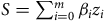 $S = \mathop \sum \nolimits_{i = 0}^m {\beta _i}{z_i}$
is also a random variable with normal distribution, whose variance can be computed as:
$S = \mathop \sum \nolimits_{i = 0}^m {\beta _i}{z_i}$
is also a random variable with normal distribution, whose variance can be computed as:
 $$Var\left[ S \right] = \mathop \sum \limits_{i = 0}^m \mathop \sum \limits_{j = 0}^m {z_i}{z_j}Cov\left( {{\beta _i},{\beta _j}} \right).$$
Given this information, a confidence interval (CI) $\left[ {{S_{{\it{min}}}},{S_{{\it{max}}}}} \right]$
for S at any given confidence level can be computed. Substituting values
$\left[ {{S_{{\it{min}}}},{S_{{\it{max}}}}} \right]$
for S at any given confidence level can be computed. Substituting values ${S_{{\it{min}}}}$
and
${S_{{\it{min}}}}$
and ${S_{{\it{max}}}}$
instead of
${S_{{\it{max}}}}$
instead of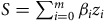 $S = \mathop \sum \nolimits_{i = 0}^m {\beta _i}{z_i}$
into (1), the CI
$S = \mathop \sum \nolimits_{i = 0}^m {\beta _i}{z_i}$
into (1), the CI $\left[ {{\lambda _{{\it{min}}}}\left( {t,z} \right),{\lambda _{{\it{max}}}}\left( {t,z} \right)} \right]$
for the mortality rate
$\left[ {{\lambda _{{\it{min}}}}\left( {t,z} \right),{\lambda _{{\it{max}}}}\left( {t,z} \right)} \right]$
for the mortality rate $\lambda \left( {t,z} \right)$
can be computed. Further, substituting
$\lambda \left( {t,z} \right)$
can be computed. Further, substituting ${\lambda _{{\it{min}}}}\left( {t,z} \right)$
and
${\lambda _{{\it{min}}}}\left( {t,z} \right)$
and ${\lambda _{{\it{max}}}}\left( {t,z} \right)$
in place of
${\lambda _{{\it{max}}}}\left( {t,z} \right)$
in place of $\lambda \left( t \right)$
in (9), the CIs for the survival probabilities can be computed. The resulting CIs depend on the input vector z, and as such these values are computed for each individual. That is to say, some individuals can have a more accurate prediction than others. The resulting CIs are included for the final models described below.
$\lambda \left( t \right)$
in (9), the CIs for the survival probabilities can be computed. The resulting CIs depend on the input vector z, and as such these values are computed for each individual. That is to say, some individuals can have a more accurate prediction than others. The resulting CIs are included for the final models described below.
6.4.3 Medical Justification Review
At all stages of our work (from attribute selection to outcome verification) we consulted with medical specialists from Leicester Diabetes Research Centre.
There is a risk with data partitioning that risk factors where there may not be a prior expectation of reasonable differentiation in the coefficient value by sex, are included. The comparisons for Cox coefficients for both models are presented in Tables 91 and 92. As we can see from Table 92, one attribute has different signs for male and female: Angina is a risk factor for males but reduces the risk of death for females. This divergence, while initially counter-intuitive, may reflect real-world clinical and diagnostic patterns. In males, angina is often an indicator of significant underlying coronary artery disease and is more likely to be associated with acute coronary events, thereby justifying its positive association with mortality risk. In contrast, for females, angina symptoms are frequently less specific, often underdiagnosed or misattributed, and may lead to more conservative management or greater healthcare engagement. As a result, women with diagnosed angina may actually represent a more health-aware, treatment-compliant subgroup, potentially explaining the observed inverse association with mortality. Therefore, although this appears a counter-intuitive differentiation in the coefficient value by sex, we do not think this poses issues with the data or analysis.
To ensure the models are not “over-fit” to the data, the sex-variation in coefficient values by each risk factor (independently and in combination) is reviewed by medical experts.
Computed coefficients do not always correspond to our intuition. For example, some diseases that are intuitively dangerous have negative influence on mortality and some attributes that are intuitively important turned out to be insignificant. Some seemingly “paradoxical” coefficients, such as, for example, the u-shaped association between BMI and mortality, have been confirmed by our colleagues from Diabetes Research Centre as meaningful and consistent with the literature. In other cases, after consulting with medical experts, the influence does not appear meaningful or consistent with the literature. For example, this is the case for the influence of coronary heart disease (CHD). These coefficients are the optimal values from a complex multidimensional optimisation problem, which is at the current time the best modelling that could be achieved with the data available. As stated in Section 4.1, it is not the objective of this analysis to establish epidemiological causation, but to identify variables that show meaningful correlations with mortality outcomes. The reader should take all results with the benefits and limitations in mind and be satisfied, based on multiple sources of information that the differentiators in mortality risk are fair and evidence-based.
6.5 Model Outputs
6.5.1 Summary of Model Output
Each of the models developed in this project are summarised on a separate tab in the Model Output Tool (an Excel document titled “Model_Output_Tool.xlsx”). There are 12 models in total, covering the combinations of sample, data partitioning and mortality estimation method summarised in Table C.
Combinations of sample, data partitioning and mortality estimation method used in the Model Output Tool

Table C Long description
The table presents a comparison of sample types, data partitioning, and mortality estimation methods used in the Model Output Tool. It consists of four rows and three columns. The columns are labeled Sample, Data partitioning, and Mortality estimation method. The rows detail the combinations for the General sample, Type 1 diabetes, and Type 2 diabetes. Each row specifies the sample type, the data partitioning by male and female, and the mortality estimation method, which is the exponential model with a homogeneous model for all samples.
For example, D2T Male Homo is a model that estimates mortality using the homogeneous model for the baseline force of mortality and is appropriate for an individual who is male with a Type 2 diabetes diagnosis. This model is built and fitted based on the DS sample data set. Models without “Homo” in the title use the exponential model (8) for baseline hazard rate.
Within the Model Output Tool, an individual’s vector ${z_i}$
can be entered to the “Input Information”. Guidance on the format and relevant period for the data is provided in the tool and is in line with Section 6.2.2.
${z_i}$
can be entered to the “Input Information”. Guidance on the format and relevant period for the data is provided in the tool and is in line with Section 6.2.2.
The Model Output Tool transforms the input information as described in Section 6.2.2 and returns the corresponding risk factor or Cox coefficients values for each attribute. The final input information required is a “Date of application”. From this set of inputs, the Model Output Tool provides the following:
-
• Covariate influence.
-
• Initial hazard influence.
-
• Time independent part of risk.
-
• Probability of death within the
$t{\rm{t}}{{\rm{h}}^{}}$
year after application, for
$t = 1,2,3,4$
. -
• Cumulative probability of death within t years after application, for
$t = 1,2,3,4$
. -
• 95% CIs for each probability of death above.
-
• The CI multiplier: a ratio of the upper to lower value in a CI.
-
• Squared SE calculated through covariance matrix: this is a variance of a normal random variable with the given CI.


The probabilities of death produced by the model meet the research objective of improving the understanding of mortality risk stratification across both the general and diabetic populations in the UK, with a particular focus on how risk factors vary by sex and disease type. This output can be helpful to the intended audience of life insurers, actuaries, medical underwriters and policy advisors, as it provides:
-
• A new source of information based on the UK general compared to diabetic population.
-
• A new source of information that allows insurers to critique existing information and understanding of the risk.
-
• A data-driven basis for more tailored underwriting practices and risk stratification, supporting product innovation and pricing refinement for individuals with diabetes.
Both time-homogeneous and time-inhomogeneous models are included in the output rather than one final preferred model, because each offers distinct insights into the nature of mortality risk, and their inclusion supports a more flexible and comprehensive analysis. Time-homogeneous models assume that the effect of risk factors remains constant over time, offering simplicity and ease of interpretation, which can be useful for baseline comparisons and traditional actuarial applications. In contrast, time-inhomogeneous models consider the improvement of medicine over time, capturing changes in risk dynamics such as age-related shifts in disease progression or impact of improved treatment. Commentary from the industry on model outputs and the benefits and limitations is provided within the Discussion in Section 7.
6.6 Benefits and Limitations of Model Outputs
The final models have both benefits and limitations.
Regarding data, routinely collected data suffers from data quality issues. As detailed in Section 4, care is taken however issues remain including but not limited to:
-
• The data are limited to England only and are restricted to the study period.
-
• As expected, most deaths happened for reasonably old individuals, say between age 70 and 90. Therefore, we did not have enough data to estimate mortality of young individuals. We also have limited data about very old individuals (older than 90, say), because not many individuals survived until this age. As a result, our mortality predictions for young individuals and for very old individuals are likely to be less accurate.
-
• Because we find that CPRD death information is often incorrect, we used only individuals linked to ONS. This reduces the number of individuals. Moreover, linked data belongs to England only, not the whole of UK. More importantly, the analysis in Table 48 shows that most of the diseases (28 out of 41) are not independent from linkage. In conclusion, using only ONS linked individuals significantly reduces the observed death counts in the data and the missingness is not independent of disease; this could introduce both hazard rate and coefficient misestimation risk.
-
• As detailed in Section 4, missing data is imputed where possible and reasonable, but imputed data are not as informative as actual values and can introduce the risk of over confidence by coefficients. Some risk factors such as IMD or Smoking status have a high proportion of inputted data. Some other risk factors had such an extent of missingness that these could not be included for analysis, but these are only considered a limitation where the risk factor usually forms an allowable insurance industry underwriting risk factor (e.g., marital status).
-
• It should be noted that, many individuals who leave the UK do not inform NHS and are still registered. The absence of diagnoses and death records appears in the data as if these individuals are all alive and have no new diseases. This is partially corrected by removing older individuals with no activity records during the study period, but in general it is not possible to reliably decide for every individual whether they are absent from observations due to migration or due to being healthy and not attending GP. Under-observation in routinely collected data occurs for various reasons. Section 4 discusses how this is allowed for where a death observation is missing. However other reasons for under observation, such as lax de-registering of individuals, are not accounted for. This may introduce bias to the results in a direction that depends on how the unobserved group differs from the remaining population. Individuals who emigrate without notifying the NHS are disproportionately younger, healthier and more mobile. Therefore, bias may be stronger in subgroups associated with higher likelihood of migration – such as younger adults, students, recent migrants to the UK, or certain socio-economic or ethnic groups – leading to differential underestimation of rates by these risk factors. Consequently, hazard ratios for risk factors correlated with migration could be biased towards the null, while comparisons involving older, less mobile groups may be less affected.
Regarding risk factor treatment and transformation:
-
• Diabetes classification, as described in Section 4, is not exact. As such, there is potential that the results are affected. Misclassification is more likely to occur in individuals diagnosed at ages near the threshold used for classification (e.g., late-onset Type 1 or early-onset Type 2 diabetes). If some Type 2 cases are misclassified as Type 1, the apparent incidence of Type 1 will be inflated and its association with risk factors more typical of Type 2 (such as obesity, lower physical activity and certain ethnic backgrounds) may be exaggerated. Conversely, if some Type 1 cases are misclassified as Type 2, the incidence of Type 2 will be overestimated in younger individuals, potentially diluting associations with classic Type 2 risk factors and biasing hazard ratios towards the null. Overall, the misclassification is likely to attenuate differences between the two Types, particularly for age and BMI.
-
• For dynamic risk factors such as BMI, BP, or CL, we took into account only the latest observation, not the whole time series. This is a limitation because single, most recent measurements, may not accurately represent an individual’s long-term exposure or trajectory. For dynamic risk factors, values can change substantially over time, and the latest observation may reflect changes caused by early disease symptoms, treatment, or temporal lifestyle changes, rather than the individual’s typical baseline status. This can introduce reverse causation bias if the latest measurement is taken after disease onset or in response to emerging health issues. It may also attenuate associations if variability over time is ignored, particularly for risk factors that fluctuate with age, season, or life events.
-
• For each disease (excluding diabetes, where duration was modelled), we utilised a binary attribute indicating whether the disease had ever been diagnosed. Consequently, this definition treats the condition as a permanent risk factor, effectively ignoring the possibility of full recovery. We justify this approach based on the chronic and progressive nature of the high-impact co-morbidities included in the model, where “recovery” to a baseline risk state is clinically rare. For episodic or acute conditions (such as stroke or cancer), we assume that a historical diagnosis serves as a permanent marker of physiological frailty and elevated recurrence risk. The statistical consequence of this approach is conservative: if a subset of “fully recovered” individuals is included in the disease group, it would dilute the association between the disease and mortality, potentially underestimating - but not overestimating - the true severity of the condition.
-
• For co-morbidities, we only take into account whether a disease has been diagnosed before the start date or not and do not take into account the date of the diagnosis. In reality, a year-old diagnosis and a 30-year-old diagnosis of the same disease may have different influence on the mortality probability.
Regarding modelling:
-
• Much of the existing literature investigates the effect of one specific attribute or several specific attributes on diabetic mortality risk. Here, a large number of attributes are investigated simultaneously and in combination. However, not allowing for the temporal aspect means that we are effectively assuming they remain constant over follow-up, which is rarely the case. Many risk factors – such as BMI, smoking status, BP and treatment use – can change significantly over time, sometimes in response to early disease processes or clinical interventions. Treating them as fixed can misclassify exposure, dilute observed associations and introduce reverse causation if post-diagnosis changes are incorrectly interpreted as pre-existing risk factors. As a result, the simultaneous modelling of many attributes may underestimate the true effects of dynamic risk factors and overstate the stability of their relationships with diabetic mortality.
-
• The Cox model explicitly shows the effect of each risk factor on mortality via the Cox coefficients. Many papers compute Cox coefficients only. Here, the baseline hazard rate is also estimated in explicit form. Therefore, the models herein provide an estimate of mortality risk over the specified time period.
-
• Most of the risk factors analysed are not independent of each other. The Cox model allows a set of attributes that are useful for estimation of mortality risk to be selected. Risk factors removed were not significant, but this does not mean that these risk factors are irrelevant. Some risk factors removed that are not statistically significant can still be used through correlation with included attributes.
-
• The significance of risk factors may depend on the order in which they are removed.
-
• Homogeneous and non-homogeneous models were developed separately for males and females, and separately for each sample; GS, Type 1 and Type 2 diabetes. The number of model types, fit by sample and extent of risk factors is more comprehensive than most of the literature.
-
• As discussed in Section 6.1.2, the Cox model assumes risk factors influence the hazard rate independently. The model herein has the benefit of including pairwise interactions. Higher order interactions were not considered to ensure the coefficient value outputs were easier to interpret. Deep learning models that represent mortality rates as complicated functions of the risk factors were not considered suitable, even though these can account for interactions of all orders and so potentially estimate mortality more accurately. This is because, for such models, the exact influence of each attribute is not transparent which was a necessary objective of the research.
Regarding model output:
-
• Modelling stages were reviewed for justification by data and medical expertise. The Cox proportional hazards model provides coefficients that adjust a baseline hazard rate – this baseline is unspecified but represents the hazard function for an individual with all covariates set to zero. What is considered “standard” in this context is not a predefined life, but rather a relative risk framework where individual hazard rates are expressed as a function of covariate effects layered on top of this baseline.
7. Discussion
To provide a meaningful discussion, it is most valuable to consider the results within the context of potential applications and gain the views of potential users of the research. To achieve this, the discussion section is provided as a general industry discussion followed by an applied industry discussion. Within this discussion section, the key discussion points from the general industry discussion roundtable event are summarised. Finally, the underwriting process is outlined to provide context for the key summary points of the applied industry discussion.
7.1 General Industry Discussion
The IFoA ARC held a roundtable event with industry practitioners on ${10^{}}$
July 2024 to discuss the commissioned work on an analysis of diabetes. The participants included insurers, reinsurers and academia to discuss the outputs of the University of Leicester model (“The Model”) from an underwriting and actuarial perspective (“the group”). Overall, the feedback from the group was that the research was considered important and a significant contribution to the insurance industry which provides insights into the complex condition of diabetes for the benefit of consumers. Specific discussions were held in the following areas and the key views summarised.
${10^{}}$
July 2024 to discuss the commissioned work on an analysis of diabetes. The participants included insurers, reinsurers and academia to discuss the outputs of the University of Leicester model (“The Model”) from an underwriting and actuarial perspective (“the group”). Overall, the feedback from the group was that the research was considered important and a significant contribution to the insurance industry which provides insights into the complex condition of diabetes for the benefit of consumers. Specific discussions were held in the following areas and the key views summarised.
7.1.1 The Data and Data Item Quality
There was a brief discussion on some of the features of the CPRD data set that required significant adjustment. Firstly, the death records on CPRD were unreliable and so data was used only when it could be linked to the ONS death records. Secondly, the adjustment at older ages which saw individuals removed above age 80 from 1 October 2010 where the GP record had not changed for a 10-year period (“the study period”). Individuals may move abroad or move GP practice outwith those included in the CPRD network. The group were satisfied with how the data issues were handled but it highlights data quality issues at older ages.
The data field to indicate the Type of diabetes within the CPRD data set is not always populated and so uncertain. It was therefore necessary, where this information was not available, to introduce an age-related assumption to determine the Type of diabetes. For a diabetes diagnosis below age 28 it was assumed to be Type 1, and for a diagnosis equal to or above 28 assumed to be Type 2. The feedback from the group was that this was a reasonable assumption to make. As childhood obesity and consequently earlier ages of developing Type 2 are increasing, this assumption could be challenged in any future iterations of the models. It is accepted this is not a perfect proxy; however it is reasonable enough not to adversely affect The Model.
HbA1c is a key metric used in underwriting to assess the risk presented by an applicant for insurance. For example, an individual diagnosed with diabetes 10 years ago who manages their diabetes well is considered to have lower mortality risk than an individual diagnosed with diabetes 5 years ago who has not maintained good control. NICE guidelines do recommend that HbA1c is recorded at least annually within GP records; however, the data does not reflect this frequency of recording. Based on insurance data, it was estimated that around 50% of applicants disclosed at the time of underwriting that they did not know their HbA1c but would characterise their diabetes management as “amazing control”, based on underwriter’s experience in the group. The Model uses the last HbA1c measure recorded whereas an underwriter may look at the last 3 years of data recorded, if available. It is expected that a recently diagnosed individual, within the last 10 years, may have much better management of their condition, reflecting better medication and insights. Acceptable control of HbA1c for access to insurance is key (between 6% and 8% as the percentage of haemoglobin in the blood that is glycosylated), particularly for Type 1. The medical definition is different where optimal control is defined as 7% (53 mmol/mol) or less.
7.1.2 The Variables of Interest, Applicability and Results
Ethnicity is an important factor for diabetes. However, it is not considered within The Model as the data item is not reliable. Further, insurance companies do not use ethnicity as a factor when setting prices in UK and Europe to comply with the Equality Act 2010. Therefore, although ethnicity is an important risk factor for diabetes, its absence in the modelling does not affect the usability for the intended users of the research.
Underwriters often use family history as a guide to the risk of the person applying for life insurance. Family history was not considered as a variable within The Model. Within GP data records, family history is a free text field and is filled in selectively for individuals with a high risk of cancer. It is more likely to be recorded where there is a family history of stroke and heart disease, than for diabetes. If diagnosed with diabetes, family history would be considered irrelevant for mortality risk; however, family history of stroke and heart disease would still have relevance when underwriting a risk.
The Group discussed the differences between Type 1 and Type 2 based on outputs from The Model:
-
• For a Type 2 diabetic, the number of years (duration) since diagnosis is a key consideration as the mortality rates increase each year by about 4% for every year since diagnosis. On the other hand, for Type 1 diabetes duration since diagnosis is less material as there is a much smaller trend from year to year. The Model also shows that if someone has Type 2 diabetes for a long time, the mortality rate is similar to Type 1. The Group thought this was reasonable.
-
• One underwriter explained that Type 1 diabetes base ratings tend to be higher than Type 2, given that the majority of applications tend to be for individuals in their mid-30s. For Type 1, complications are likely to have an impact at an earlier age given the individual is diagnosed at a much younger age. The only time when Type 2 is higher is if there is poor control and significant complications from co-morbidities. Generally, a Type 2 diagnosis tends to occur over the age of 45, so the cause of death is likely to happen in the next 35 years. The risk of developing Type 2 diabetes increases with age. Below the age of 45, it is estimated to be
$1.5{\rm{\% }}$
of the population and above this, increasing from 8% to 20% as age increases.Footnote
11

The Model results indicate gender is an important predictor of mortality risk for those living with diabetes. With regard to the diabetes population, overall it is seen that females with Type 1 diabetes have higher mortality than males, in contrast to the general sample. On the other hand, in Type 2 diabetes, males and females are more aligned. Women lose their pre-menopausal cardiovascular protection with age and so become closer to the males. Younger females with Type 1 tend to have poorer control.
BMI is considered to be an important variable in relation to diabetes mortality risk. The Model produced the expected U-shaped graph.Footnote 12 The exception is female with Type 1 diabetes with BMI 20-39, which showed a relatively flat relationship with expected mortality rate by BMI category. The Group considered that the impact of BMI is likely minimal when other health problems are not present, but The Model does indicate that BMI is important as a factor.
SES is considered to have a material impact on mortality risk. Often, IMD is used as a SES proxy. Within the Model, the IMD is based on the postcode of the individual, or the GP postcode in over 50% of cases where individual postcode is not present. For the diabetes population, there is a distinct increase in mortality for males with diabetes from affluent to less affluent. This is not as apparent for females with diabetes; the mortality risk is relatively flat by IMD. However, the CIs are wide so care must be exercised in drawing any firm conclusions. The general sample population has a slight increase by IMD. Affluent males do have lower risk, possibly due to better access to health care services and being more aware of health issues. It was discussed why affluent females, on the other hand, do not benefit from affluence which could be due to females being generally better engaged with health services across socio-economic groups.
Co-morbidities are an important indicator of mortality risk for the general and the diabetes populations as can be seen in The Model results. The co-morbidity attributes in The Model are a complex area to understand given the large number of possible co-morbidities and the interactions involved. The group’s key discussion points are summarised below:
-
• Heart failure has the largest impact on the general sample followed by Type 2 and then Type 1. This is due to the relative increase in
${q_x}$
for the different populations where the general sample has the lowest
${q_x}$
followed by Type 2 and then Type 1. -
• CHD does not have an impact on the general sample but does for females with diabetes. For males, there is no impact due to the interaction with hypertension. The model does not include the severity of the co-morbidity case. As discussed, this highlights a deficiency in the model that could be improved by pre-defining CHD as a standard condition to be modelled.
-
• In underwriting, a member of the group at the roundtable event anecdotally stated that about
$15 - 20{\rm{\% }}$
of applicants for life insurance declare a second condition, which is lower than what The Model shows. Underwriters receive targeted reports for diabetes which may not pick up other complications and those applicants not declaring; however, the model does utilise other factors such as BMI. -
• There was interest in the cumulative impact of co-morbidities. Traditionally, some underwriters treat BMI and diabetes separately, but data does reveal a different impact if combined. The model does allow for pair-wise interactions. But, the model is limited in its data treatment for within-study-period disease diagnoses and co-morbidities.
-
• Type 2 diabetes and BMI can be reversed but lifestyle changes are difficult and there is an epigenetic legacy with diabetes. Remission is rarely achieved and rare to maintain.
-
• There was a suggestion of further research looking at the pathway from diagnosis to heart disease event, kidney failure, etc. to inform critical illness cover.


7.1.3 The Final Models and Practical Use
In the discussion, both models homogeneous and non-homogeneous were discussed. The homogeneous model was considered more reliable than the non-homogeneous model, which includes a trend factor over time. The non-homogeneous model was based on only 10 years of data, which was considered an insufficient period to establish a trend.
7.2 Applied Industry Discussion
To gain the views of potential users of the research in an applied sense, a subgroup of the roundtable discussion was asked to review a set of example applicants with diabetes profiles and share their underwriting outcome for comparison to the final models. Fifteen pre-constructed applicants with diabetes customer profiles (“example cases”) were agreed with 5 profiles for Type 1 diabetes and 10 for Type 2. The example cases were derived based on realistic cases reinsurers underwrite. The subgroup from the roundtable asked to participate in the applied industry feedback was composed of the reinsurers present (“the participants”). This is considered indicative of the industry, as direct insurers frequently defer underwriting outcomes ratings to be based on reinsurers’ manuals. Therefore, inclusion of all members of the group at the roundtable would have led to bias; results duplication where one or more reinsurers’ underwriting manuals are used.
To provide context for the applied industry discussion below, first the underwriting process is outlined in general:
-
• Applicants applying for insurance are subject to an underwriting process where many attributes are considered. If the applicant has diabetes, further information is requested such as: Type of diabetes; duration since diagnosis; HbA1c; BMI; and any co-morbidities (Table 109).
-
• The term “healthy lives” herein refers to applicants without a diabetes diagnosis and no pre-existing health issues from the list of co-morbid conditions used in The Model. These individuals also have: a BMI in the range 20–25, an IMD of 1 (most affluent group), Systolic/Diastolic Blood pressure in the range 90–120 and 60–80 respectively, and, finally, total CL less than or equal to 5 mmol/L.
-
• Generally, and in simplified terms, “healthy lives” would be accepted as a result of the underwriting process without the need for additional underwriting outcomes to be applied. When an applicant is accepted without additional underwriting outcomes, standard rates are considered appropriate, that is, these applicants are accepted on healthy lives expected mortality (“healthy lives
${q_x}$
”). -
• Generally, and in simplified terms, applicants with pre-existing health issues such as a diagnosis of diabetes, may be accepted as a result of the underwriting process with the additional underwriting outcomes applied. When an applicant is accepted with additional underwriting outcomes, non-standard rates may be considered appropriate, that is, these applicants are accepted with a rating above the healthy lives expected mortality (“rated lives
${q_x}$
”). For example, an applicant with diabetes may have a higher premium to compensate for the higher expected mortality. -
• Alternative terms are available but as an ultimate decision, if the mortality risk is assessed to be excessive (e.g., a rating of
$ + 300{\rm{\% }}/400{\rm{\% }}$
above healthy lives expected mortality) then the underwriting outcome may be to decline the application for death insurance benefits.



The “ratings” applied above the “healthy lives ${q_x}$
” are the underwriting outcomes the participants were asked to share for the example cases. In order to comply with competition law, the IFoA collected the information and retained confidential information:
${q_x}$
” are the underwriting outcomes the participants were asked to share for the example cases. In order to comply with competition law, the IFoA collected the information and retained confidential information:
-
• Only the perceptions of additional risk posed are shared. This removes the risk of sharing either premiums or healthy lives rates.
-
• The underwriting outcomes are anonymised and only shared when at least 2 participants haven’t declined.
-
• Only the final analysis and conclusions are published.
These outcome decisions were aggregated, for example, cases to enable comparison to Model results. Where a participant’s underwriting decision would be to accept with a rating applied, the average rating is shown and a range given in Table 110. The number of participants who would decline is also shown; where the number of declines is high then no average rating is shown (where only 1 reinsurer rating is available).
Results of the University of Leicester model (“The Model”) are applied to the example cases. Where co-morbidities are present, these are input to The Model where there is an option to select it. The output from The Model is based on the following:
-
• A separate average ratio for males and females of the rated-lives mortality
$q_x^{{\rm{rated}}}$
to the healthy-lives mortality
$q_x^{{\rm{healthy}}}$
over 10- and 20-year periods. The mortality rates are projected by cohort, for example, age 27 duration 0 will be age 28 duration 1 a year later. A weighting is applied to the rating by
$q_x^{{\rm{healthy}}}$
to allow for the impact of mortality increasing with age. -
• Only the homogeneous model rather than the non-homogeneous model is used. This is appropriate as the homogeneous model has no time trend (e.g., a policyholder aged 26 with duration 0 is treated the same as one aged 25 duration 1, which is equivalent to age 24 duration 2, etc.).
-
• To calculate the rating, a general sample of healthy lives (baseline with no loadings by smoker status) is compared to The Model results for Type 1 or Type 2 diabetes.


To enable a reasonable comparison, insured lives tend to be more affluent than the general population which in turn means that insured lives have on average lower levels of mortality compared to the general population. This occurs due to the well-established correlation between mortality and socio-economic determinants. This is an important factor in explaining inequalities in life expectancy; life expectancy is significantly lower in more deprived areas compared to less deprived areas in England. In order to allow for the discrepancy in expected mortality and therefore proxy the expected mortality of the insured lives sample, the IMD of 1 (scale is from 1 to 5 where 1 is the most affluent) is used in the example cases. This is not precise because the general population sample used in this research as a benchmark will have different experience compared to an insured population across different ages and genders.
7.2.1 Key Summary of Comparison
7.2.1.1 In general
An underwriting decision is based on the health of the applicant at the time of application. The resulting rating applied to the standard rate expected mortality is applied throughout the duration of the contract which could be over 25 or more years. In comparison, The Model provides a projected ${q_x}$
, which develops over time.Footnote
13
Therefore, these two methods can be compared to assess how the ratio
${q_x}$
, which develops over time.Footnote
13
Therefore, these two methods can be compared to assess how the ratio $q_x^{{\rm{rated}}}/q_x^{{\rm{healthy}}}$
changes over the duration of the contract, that is, how the rating varies over time. The outcome of The Model is that ratings tend to reduce over time as the policyholder ages. This is something the industry could also consider as ratings are normally based on the health of the applicant at the time of underwriting and not over the term of the life contract (up to 25 years and beyond).
$q_x^{{\rm{rated}}}/q_x^{{\rm{healthy}}}$
changes over the duration of the contract, that is, how the rating varies over time. The outcome of The Model is that ratings tend to reduce over time as the policyholder ages. This is something the industry could also consider as ratings are normally based on the health of the applicant at the time of underwriting and not over the term of the life contract (up to 25 years and beyond).
7.2.1.2 Specifically for Type 1
The average ratings produced by The Model for Type 1 diabetes are within range of the underwriting ratings for cases 1, 2 and 4 where the number of declines is 0 or 1 (Table 110). Male outcomes from The Model tend to be at the lower end of the range compared to the average rating of the participants’ underwriting outcomes; whereas female outcomes from The Model are much higher above the upper rating.
It is also observed that the participants’ ratings are highly variable with a wide range, which illustrates that each has a different view of the risk. A varying view of the risk may occur when there is a highly uncertain estimate, or different participants have different sources of information for the basis of the risk perception.
The use of the applicant’s gender by participants in the risk assessment of diabetes is not used. This may reflect greater sensitivities on the use of gender created by the EU Gender Directive, even though the guidance indicating its use would be acceptable in relation to the different health outcomes. The Model rating is lower when comparing the 20-year average to a 10-year average. The rating for ${q_x}$
reduces as the applicant gets older. The 20-year average model rating is either close or below the lower rating range for males.
${q_x}$
reduces as the applicant gets older. The 20-year average model rating is either close or below the lower rating range for males.
For cases 3 and 5, the risk is considered high and is declined by most of the participants. In these cases, we do have higher ratings generated by the model compared to cases 1, 2 and 4. In the example cases with co-morbidities (cases 3, 4 and 5), the model does not explicitly include chronic kidney disease, retinopathy, peripheral vascular disease, or diabetic neuropathy. The reason for this is due to high correlation of these conditions with other co-morbidities, particularly hypertension (Tables 55 and 56). A learning for future model iterations would be to design the selection of co-morbidities so the model includes these key co-morbidities for diabetes as standard. This would provide more refinement than using the broader hypertension condition.
7.2.1.3 Specifically for Type 2
The Model has much lower ratings for Type 2 diabetes compared to the participants’ ratings. This is across all Type 2 diabetes example cases from 6 through to 15.
A plausible explanation for this is due to the underwriting process. Those applicants that are successful and go through the process to be accepted will be healthier, that is with a lower ${q_x}$
compared to a healthy sample from the general population sample. The healthy sample from the population will include individuals with diabetes and other conditions that have not been diagnosed yet through either a visit to their GP or hospital.Footnote
14
The insured population will be healthier as there is a selection process to categorise lives into healthy lives, rated lives and, where risks are too high, would be declined. This difference may explain why a small difference is seen between a healthy general sample and a sample of Type 2 diabetes for each case for The Model outcomes. Also, those diagnosed with diabetes will be receiving treatment and general health checkups which may reduce the mortalityFootnote
15
against a general sample that includes individuals that have undiagnosed diabetes without treatment.
${q_x}$
compared to a healthy sample from the general population sample. The healthy sample from the population will include individuals with diabetes and other conditions that have not been diagnosed yet through either a visit to their GP or hospital.Footnote
14
The insured population will be healthier as there is a selection process to categorise lives into healthy lives, rated lives and, where risks are too high, would be declined. This difference may explain why a small difference is seen between a healthy general sample and a sample of Type 2 diabetes for each case for The Model outcomes. Also, those diagnosed with diabetes will be receiving treatment and general health checkups which may reduce the mortalityFootnote
15
against a general sample that includes individuals that have undiagnosed diabetes without treatment.
However, the rating for case 6 should be near a healthy life as this life has no co-morbidities, that is, the only diagnosis is Type 2 and with good control of HbA1c. This example case is overweight with a BMI of 37, but this variable within The Model does not lead to a predicted higher mortality at older ages. The average participants rating is around $ + 100{\rm{\% }}$
.
$ + 100{\rm{\% }}$
.
Another feature to explain why the resulting ratings in the model are lower for Type 2 diabetes is to consider the HbA1c metric. The HbA1c measure for all the example cases is between 5.7 and 10, which reduces the risk of mortality compared to levels outside this range. The model does show a typical U-shaped curve where below 5.7 and above 10 shows higher mortality. The calibration of the model could be more refined.
Most participants declined example cases 10, 13, 14 and 15. This is predominantly due to the serious co-morbidities associated with these cases and the HbA1c readings were towards the higher range. The model here gives a result that is close to a 0 rating. This highlights a deficiency in the model in that the co-morbidities are based on a single average factor based on the data using a proportional Cox model, so refinements such as the severity of the co-morbidity are not captured. The model is also based on the latest readings and not an average that can provide more information on the variability for certain measures such as HbA1c. Other factors that will have a significant influence on the results are the individual pathway for co-morbidities, such as treatments and drugs. These factors are not captured by the model.
7.3 Further Work Since Discussion
There were some significant challenges made to the findings:
-
• Ratings for females are very high compared to males for Type 1 diabetes.
-
• Ratings for Type 2 that resulted in negative loadings where there are potentially very serious co-morbidities/complications present.
Further work was carried out to address the latter point. A simplified model was created, exploring a noted limitation to the model, namely the ordering of risk factors when fitting the model. In this exploratory work, the order in which co-morbidities are added into the model was altered, and we only included important co-morbidities for individuals with diabetes. The order we proposed was as follows: CHD, stroke, chronic kidney disease, peripheral vascular disease, diabetic neuropathy, retinopathy, hyperlipidemia, amputation and hypertension.
The purpose of this exploratory modelling was to check the significance of this limitation, as well as the significance of these diseases for mortality prediction without other co-morbidities. This additional modelling does suggest that of the co-morbidities tested, all are significant including CHD, stroke, MVD, blindness, amputation and finally hypertension.
Therefore, when fitting the model there are significant important model design choices in terms of which co-morbidities are included and the ordering of the risk factors. We suggest having co-morbidities retained that are most relevant for individuals with diabetes and factored into the model in the order of importance for individuals with diabetes.
This exploratory model is an initial step and further work in the model design would be required to overcome the challenges made.
7.4 Conclusion
The general industry and applied industry discussions provided context to the results through the example cases, based on typical cases underwritten where the applicant has diabetes.
The following insights were discussed:
-
• BMI exhibited a U-shape, which is aligned with what underwriters would expect to see.
-
• IMD exhibited a different pattern for males compared to females, where males have a much stronger increase in mortality rates as IMD goes from affluent to less affluent but on the other hand the pattern for females was not well defined; however, CIs were wide.
-
• A useful insight provided by the reinsurer loadings is the variation in ratings between the reinsurers based on a different view of the risk.
-
• It was also interesting that the model loadings depend on the period the rating is applied for, as the rating tends to reduce over time as the population ages.
-
• The model results for Type 1 were within the range of the underwriting results, except for female where they are much higher. This was challenged, but underwriters typically use gender neutral ratings so a benchmark was not possible.
-
• Type 2 results were challenged as some of the more serious co-morbidities were not adhering to prior expectations. Further exploratory modelling work suggested the order and sequence of the key co-morbidities for diabetes is important.
-
• Overall, the patterns between different factors were aligned with expectations.
The modelling was appreciated in the general discussion but there are many complications such as the quality of the data and how to handle co-morbidities correctly. Building a general model that covers Type 1 and Type 2, and all the different co-morbidities was ambitious. We understand this is the first time that has been done. The general feedback was that creating a model based on CPRD data was worthwhile as an initial approach that can be improved upon based on the feedback from practitioners. This research therefore provides a useful discussion point and an additional data-driven source of information for the intended audience but it is not yet a sole source of the understanding of diabetes mortality risk.
Supplementary material
The supplementary document “Diseases influence on mortality rates” is available at https://doi.org/10.1017/S1357321726100439.
Acknowledgements
Steering Group
The purpose of the project Steering Group was to ensure that the project delivered research outputs that are of a high quality and in line with expectations, producing findings that are relevant to the actuarial community, industry and other key stakeholder groups. Ian Catchpole chaired this group (initially Nicky Draper was a Chair).
The project Steering Group included representatives from partner organisations. Independent academic guidance was provided by Professor Les Mayhew from Bayes Business School, City St George’s, University of London.
Technical Sub-group
Given the complex nature of this research, a Technical Sub-group was set up to provide additional oversight and input. Members of this group included: Scott Reid, Wui Hua (John) Ng, Mei Sum Chan, Roshan Tajapra, Han Yan, Kishan Bakrania, Jon Lambert and Chris Bagnall.
Industry Discussion
The roundtable event held on the 10 July 2024 was conducted under Chatham House Rules. This was to encourage openness in the discussion. The insurance/reinsurance companies represented were as follows: Zurich, L&G, SCOR, Partner Re, RGA, Hannover Re, Gen Re, Munich Re and Pacific Life Re. Swiss Re provided written feedback post event. Academic institutions represented included the University of Leicester and Bayes Business School. Nicky Draper from Crystallise Ltd. attended given her medical expertise; previously she was Co-Chair of the Diabetes Working Party.
The industry feedback and challenge were extremely valuable, and we would like to thank those who took part in this event. Section 7 covers details of this general industry discussion and the applied industry discussion based on example cases post roundtable event.
Leicester Diabetes Research Centre
At all stages of our work (from attribute selection to outcome verification), we consulted specialists from the Leicester Diabetes Research Centre, in particular Dr Joseph Henson, who provided substantial guidance throughout the project.
The Shiny App
We thank Maros Bobulsky for developing (together with Scott Reid) the Shiny App, to make the outputs more accessible to a wider audience.
Independent peer reviewer
Josephine Robertson provided independent peer review and edited/re-drafted many of the sections. This work was invaluable to challenge and increase the quality of the overall paper. We also thank Pacific Life Re and Gen Re, who provided extensive feedback on the paper and model.
All tables and figures referenced herein can be found in a separate “Tables and Figures” document, which is located at https://vle.actuaries.org.uk/course/view.php?id=2379§ion=6.





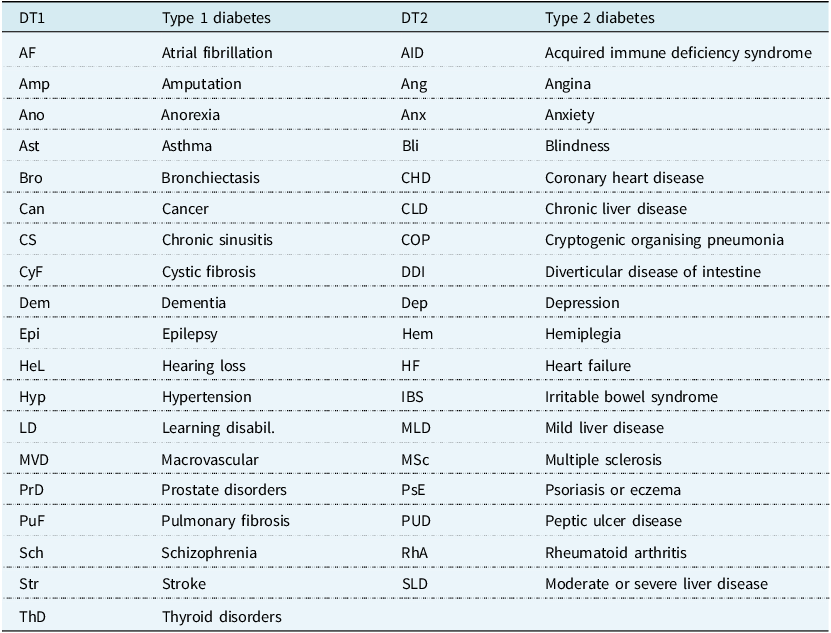




 Open access

