


Impact Statement
Because of the high costs of real engine testing and the long turnaround times of high-fidelity simulations, engineers have to rely on cost-effective tools like Reynolds averaged Navier--Stokes (RANS) for flow diagnostics and analysis. The RANS is a low-fidelity tool and therefore requires calibration/anchoring before its use for complex flows. For slot film cooling applications, RANS model calibration/anchoring heavily relies on experimental data, which gives limited access to the flow field. For inter-platform misalignment with cooling flow, obtaining simultaneous measurements of momentum and thermal fluxes close to the wall is difficult. Direct numerical simulations (DNSs) offer access to three-dimensional flow fields and all flow quantities as a function of space and time and therefore are ideal for RANS model calibration and validation. This work showcases DNSs at practically relevant flow conditions. We study the effects of forward and backward misalignments and leakage flow rates. The DNS data, which are made available along with the paper, can be used for RANS model calibration and validation.
1. Introduction
Aviation gas turbine engines power nearly all commercial flights, consume approximately 1.7 million barrels of jet fuel per day (EIA, 2021), and are responsible for much of the pollutant in the atmosphere (Reference SawyerSawyer, 1972). In the past several decades, there have been continuous efforts to make aircraft engines more efficient (Reference JonesJones, 1978; Reference Masiol and HarrisonMasiol & Harrison, 2014). A large emphasis is on increasing the temperature entering the turbine section (Reference Peters, Kumpfert, Ward and LeyensPeters, Kumpfert, Ward, & Leyens, 2003), as this directly increases the thermodynamic efficiency of the engine. In today's engines, the temperature of the incoming air from the combustor to the turbine's first stage vanes is well above the melting temperature of current nickel-based alloys, requiring significant cooling for safe operation. An extensively employed cooling technology is film cooling (Reference Bogard and TholeBogard & Thole, 2006). Consider, e.g. an engine as sketched in figure 1. The combustor annulus and the turbine annulus are cast and then assembled, leading to a gap between the combustion chamber and the turbine. A cold stream of air, originating from an extraction point in the compressor upstream of the combustor, is supplied through the gap to prevent hot gas ingestion and to protect the downstream turbine vanes from the hot gas. Thermal expansion or assembly tolerances of the engine parts often result in misaligned platforms, leading to a forward misalignment configuration or a backward misalignment configuration, as sketched in figure 1.
A sketch of an aircraft engine (GE, 2013) and a zoomed-in view of the inter-platform gap.

While a large volume of literature exists on slot cooling and inter-platform leakage flow, see e.g. Reference Fitt, Ockendon and JonesFitt, Ockendon, and Jones (Reference Fitt, Ockendon and Jones1985), Reference Popovíc and HodsonPopovíc and Hodson (Reference Popovíc and Hodson2013a), Reference Popović and HodsonPopović and Hodson (Reference Popović and Hodson2013b) and Reference Lynch and TholeLynch and Thole (Reference Lynch and Thole2017), heat transfer downstream of a platform misalignment has received very limited attention. Reference Cardwell, Sundaram and TholeCardwell, Sundaram, and Thole (Reference Cardwell, Sundaram and Thole2005) are among the first to investigate the effects of platform misalignments. The authors conducted a wind tunnel experiment and reported notable effects of platform misalignment on end wall heat transfer. Specifically, the authors noted increased cooling effectiveness for the backward misalignment configuration and decreased cooling effectiveness for the forward misalignment configuration. In a later experimental study, Reference Piggush and SimonPiggush and Simon (Reference Piggush and Simon2007) considered a contoured end wall and found that, compared with the aligned configuration, the forward misalignment configuration increases heat flux at the leading edge of the platform, and the backward misalignment configuration slightly decreases the heat flux. Detailed measurements of the flow in the vicinity of the inter-platform gap were not available in either Reference Cardwell, Sundaram and TholeCardwell et al. (Reference Cardwell, Sundaram and Thole2005) nor Reference Piggush and SimonPiggush and Simon (Reference Piggush and Simon2007). The lack of near-wall data motivated computational work. Reference Lange, Lynch and LewisLange, Lynch, and Lewis (Reference Lange, Lynch and Lewis2016) compared their Reynolds averaged Navier--Stokes (RANS) with Reference Cardwell, Sundaram and TholeCardwell et al.'s (Reference Cardwell, Sundaram and Thole2005) and their own experiments and noted a number of RANS's inadequacies. In another RANS study, Reference Kim, Chung, Rhee and ChoKim, Chung, Rhee, and Cho (Reference Kim, Chung, Rhee and Cho2016) reported the cooling effectiveness as a function of the misalignment's size. However, because of the low-fidelity nature of the tool, the authors could not get too many insights into the flow physics. To gain a physical understanding of the flow, Reference Rao and LynchRao and Lynch (Reference Rao and Lynch2021) conducted a wall-resolved large-eddy simulation for the forward misalignment configuration. The authors compared the flow with that in the vicinity of a forward-facing step and concluded that flow injection leads to high turbulence generation when there is a forward misalignment. However, because the injection flow's temperature is the same as the free-stream temperature, the authors could not directly conclude about the heat transfer downstream of an inter-platform misalignment, where the leakage flow's temperature is usually not the same as that of the incoming flow. In all, high-fidelity data are needed for model calibration and for gaining an improved physical understanding.
The above discussion brings us to direct numerical simulation (DNS). A DNS resolves all turbulent eddies and gives access to the time-resolved three-dimensional velocity and temperature fields, thereby allowing one to compute any flow statistics. However, DNS is not possible for a lot of engineering flow problems because of its high cost at practical Reynolds numbers (Reference Choi and MoinChoi & Moin, 2012; Reference Yang and GriffinYang & Griffin, 2021), and its use in the turbomachinery industry is not common, see e.g. Reference Wheeler, Sandberg, Sandham, Pichler, Michelassi and LaskowskiWheeler et al. (Reference Wheeler, Sandberg, Sandham, Pichler, Michelassi and Laskowski2016), Reference Zhao and SandbergZhao and Sandberg (Reference Zhao and Sandberg2020) and Reference Zhao, Akolekar, Weatheritt, Michelassi and SandbergZhao, Akolekar, Weatheritt, Michelassi, and Sandberg (Reference Zhao, Akolekar, Weatheritt, Michelassi and Sandberg2020) for a few examples. Here, we are able to do DNS because the Reynolds number of the flow is not very high. In Reference Cardwell, Sundaram and TholeCardwell et al. (Reference Cardwell, Sundaram and Thole2005) and Reference Lange, Lynch and LewisLange et al. (Reference Lange, Lynch and Lewis2016), the authors matched to engine conditions and the flow's Reynolds number is  $Re_{in}=U_0C/\nu =O(10^5)$, where $U_0$ is the free-stream velocity, $C$ is the chord length and $\nu$ is the kinematic viscosity. The height of the incoming boundary layer is approximately $\delta =0.1 C$, and therefore the above Reynolds number corresponds to a Reynolds number of $Re_{b}=U_0\delta /\nu =O(10^4)$ for the incoming boundary layer: this is quite moderate, and DNSs of boundary layers at this Reynolds numbers are reported in Reference Schlatter and ÖrlüSchlatter and Örlü (Reference Schlatter and Örlü2010) and Reference Pirozzoli, Grasso and GatskiPirozzoli, Grasso, and Gatski (Reference Pirozzoli, Grasso and Gatski2004). Aside from the incoming boundary layer, the Reynolds number of the leakage jet is not high either. The gap width is $d=O(0.01C)$ and the velocity of the leakage flow is $U_j<0.5 U_0$. It then follows that the Reynolds number of the leakage flow is $Re_{j}=U_j d/\nu =O(10^3)$, which is in the laminar regime.
In anticipation of the results in § 3, also relevant are papers on forward-/backward-facing steps (Reference Fang, Tachie and BergstromFang, Tachie, & Bergstrom, 2021; Reference Hattori and NaganoHattori & Nagano, 2010; Reference Le, Moin and KimLe, Moin, & Kim, 1997), passive scalar transport (Reference Alcántara-Ávila and HoyasAlcántara-Ávila & Hoyas, 2021; Reference Kim and MoinKim & Moin, 1989) and jet flow (Reference Muppidi and MaheshMuppidi & Mahesh, 2007, Reference Muppidi and Mahesh2008), which share similar physics to the flow studied here. A detailed review of these papers, however, falls outside of the scope of this work. The rest of the paper is organized as follows. We present the detailed computational set-up in § 2. The DNS results are presented in § 3, followed by RANS results in § 4. Finally, conclusions are given in § 5.
2. Simulation details
Figure 2 is a sketch of the flow. We consider two blowing ratios  $M=U_j/U_0=0.2$, $0.5$ (the density ratio of the coolant and the hot incoming flow is approximately 1), and three step sizes $h=-0.25d$, $0$,
$0$,  $0.25d$, where $h=0$ corresponds to an aligned configuration, and $h=\pm 0.25d$ is a moderate misalignment. Table 1 lists all $M$ and $h$ values in our DNSs. The nomenclature of the cases is as follows: (misalignment)-M[ $M$], where (misalignment) is FWD, i.e. forward misalignment, FLT, i.e. no misalignment, BWD, i.e. backward misalignment, and the blowing ratio is $M=0.2$ or 0.5. The length of both the upstream plate/platform and the downstream plate/platform is $L_1=L_2=30d$, and the plates’ width is $L_z=8d$. The size of the leakage flow feed is $L_f=3d$.
Schematic of the flow configuration. The origin of the  $x$ coordinate is at the centre of the gap, and the origin of the $y$ coordinate is at the upper surface of the upstream plate.

A list of the blowing ratio and the step size in the DNSs.

We use the finite volume code CharLES for our DNSs. The code is developed at the Center for Turbulence Research and Cascade Technologies, Inc. The code solves the full compressible Navier Stokes equation, and is fourth-order accurate in space and third-order accurate in time. CharLES has been extensively used for wall-bounded flow calculations, see e.g. Reference Ma, Yang and IhmeMa, Yang, and Ihme (Reference Ma, Yang and Ihme2018), Reference Yang, Xu, Huang and GeYang, Xu, Huang, and Ge (Reference Yang, Xu, Huang and Ge2019) and Reference Xu, Altland, Yang and KunzXu, Altland, Yang, and Kunz (Reference Xu, Altland, Yang and Kunz2021a). Further details of the code can be found in Reference Khalighi, Ham, Nichols, Lele and MoinKhalighi, Ham, Nichols, Lele, and Moin (Reference Khalighi, Ham, Nichols, Lele and Moin2011) and Reference Bermejo-Moreno, Campo, Larsson, Bodart, Helmer and EatonBermejo-Moreno et al. (Reference Bermejo-Moreno, Campo, Larsson, Bodart, Helmer and Eaton2014) and the references cited therein.
We use a grid of size  $N_x\times N_y\times N_z=951\times 176\times 260$. The $y$ grid is stretched, and the top boundary is at $y=20d$. Following the previous DNSs (Reference Leonardi and CastroLeonardi & Castro, 2010; Reference Muppidi and MaheshMuppidi & Mahesh, 2007), the grid resolution is such that ${\rm \Delta} x/\varDelta _\nu <14$, ${\rm \Delta} y_w/\varDelta _\nu <1$, ${\rm \Delta} y_c/\varDelta _\nu =6$, ${\rm \Delta} z/\varDelta _\nu <6.5$, where $\varDelta _\nu$ is the viscous scale at the inlet (the viscous length scale is an increasing function of $x$),
$x$),  ${\rm \Delta} y_w$ is the wall-normal grid resolution at the wall, ${\rm \Delta} y_c$ is the wall-normal grid resolution at the top of the boundary layer. The grid resolution is ${\rm \Delta} x/\varDelta _\nu =2$ at $x=\pm 0.5d$ to accommodate the two mixing layers. We also report our grid resolution in Kolmogorov scale. The flow far upstream and downstream of the leakage is approximately boundary layer flow. The grid resolution is such that $\varDelta _x/\eta <14$, ${\rm \Delta} y_w/\eta <1$, ${\rm \Delta} y_b/\eta <5$, ${\rm \Delta} z/\eta <6.5$ – this is rather typical. In the vicinity of the the leakage, the grid resolution is such that $\varDelta /\eta <4$. Figure 3(a) is a zoom-in view of the grid in the direct vicinity of the gap, and figure 4 shows the grid resolution at $x=\pm 0.5d$ for case FWD-M5.
(a) A sketch of the grid in the direct vicinity of the gap. Here, we plot every third grid point in both the  $x$ and the $y$ directions. (b) Velocity profiles at $x=-6d$ in FWD-M5. The thin lines correspond to $U^+=y^+$ and $U^+=1/\kappa \log (y^+)+B$, where $\kappa =0.39$, $B=4.3$ (Reference Marusic, Monty, Hultmark and SmitsMarusic, Monty, Hultmark, & Smits, 2013). (c) A sample time history of the wall stress on the downstream plate in FLT-M5.

Grid resolution at (a)  $x=-0.5d$ and (b) $x=0.5d$. Here, $\eta$ is the local Kolmogorov length scale. The dip in $\varDelta _y$ at $y=0.25$ in (a) is a result of mesh refinement at the downstream wall, see figure 3(a).

The boundary conditions are as follows. The inflow is a  $Re_\theta =677$ fully developed boundary layer (Reference Schlatter and ÖrlüSchlatter & Örlü, 2010). The free-stream Mach number is approximately 0.1. Here, we briefly explain our choice of the Mach number. Most gas turbine combustors use deflagration combustion, which requires relatively low air velocities of Mach number $Ma <0.1$ to avoid blowing out the flame (Reference FerrariFerrari, 2014). The heated flow into the first stage vane is accelerated somewhat as the gas expands and the cross-section area reduces, but never generally above $Ma \approx 0.3$. The above is why we have limited ourselves to a low Mach number. The boundary layer height is $\delta _0=d$ at the inlet, and a synthetic method is employed for inflow generation (Reference Xie and CastroXie & Castro, 2008). The synthetic turbulence takes a travel distance before it could be considered as ‘realistic turbulence’. This distance varies from code to code and from application to application (Reference WuWu, 2017). Here, we anchor the flow at a distance shortly upstream of the gap. Figure 3(b) shows the mean flow at $x=-6d$ ( $24.5d$ downstream of the inlet) in FWD-M5, and the profile compares well with the logarithmic law of the wall. The results in other DNSs are similar and are not shown here for brevity. The statistics in figure 3(b) as well as the ones in § 3 are averaged in the $z$ direction and in time for approximately $T=400d/U_0$ after the flow reaches a statistically stationary state. Figure 3(c) shows a sample time history of the viscous stress on the downstream plate in FLT-M5. The signal fluctuates around its mean, suggesting that the flow is statistically stationary. Again, the results in other DNSs are similar and are not shown here for brevity. The leakage flow is a fully developed laminar channel flow. All walls are adiabatic. The adiabatic wall temperature corresponds to the temperature of the gas immediately above the metal surface in real-world engine operations. Knowledge of that temperature is critical to the subsequent design of internal cooling, and this is why an adiabatic condition is often used in film cooling calculations (Reference Bogard and TholeBogard & Thole, 2006). Last, we use a non-reflective outlet and a zero-gradient top boundary. The reader is directed to the supplemental material for additional grid and inflow information.
3. Results
The basic flow phenomenology is sketched in figure 2. A windward mixing layer emerges at the front edge of the gap, and a leeward mixing layer at the rear edge. The flow separates at the leading edge of the downstream plate, leading to a recirculation bubble. The cold leakage flow covers the downstream plate and protects it from the hot incoming gas.
First, we report the cooling effectiveness and the skin friction coefficient, which are most relevant for engineering operation. Figure 5 shows the cooling effectiveness  $\eta =(T_h-T_w)/(T_h-T_c)$ and the skin friction coefficient $C_f=2\bar {\tau }_w/(\rho _0 U_0^2)$ on the downstream plate, where $T_h$ is the temperature of the hot free stream, $T_c$ is the temperature of the cold leakage flow, $T_w$ is the adiabatic wall temperature and $\rho _0$ is the free-stream density. The cooling effectiveness is a decreasing function of the streamwise coordinate. The higher blowing ratio, i.e. $M=0.5$, brings more cold fluid into the flow field, resulting in higher cooling effectiveness far downstream of the gap, i.e. $x/d>20$, where the flow is sufficiently developed and the skin friction coefficients in all cases collapse. The higher blowing ratio also gives rise to a larger separation bubble, as we can see in table 2. The separation bubble blocks the cold leakage flow in the near field, i.e. $x/d<10$. As a result, the higher blowing ratio, i.e. $M=0.5$, leads to lower cooling effectiveness in the near field for the same misalignment configuration. The plates’ misalignment has a notable effect on the cooling effectiveness in the near field. The backward misalignment configuration leads to higher cooling effectiveness than the aligned configuration, and the aligned configuration than the forward misalignment configuration. Compared with the cooling effectiveness, the skin friction is much less affected by the misalignment. The sizes of the separation bubbles are similar in the aligned configuration and the backward misalignment configuration; the forward misalignment configuration leads to a slightly larger separation bubble. Aside from the above basic flow phenomenology, getting an empirical correlation that maps $h$,
$h$,  $M$ directly to $\eta$ and $C_f$ would be very useful, but it cannot be done with just six DNSs – a task we will leave for future investigation.
(a) Cooling effectiveness and (b) skin friction as a function of the streamwise coordinate.

The size of the separation bubble measured by the distance from the leading edge of the downstream plate to the flow reattachment location. Here, the flow reattachment location is where  $C_f=0$.

Next, we examine the mean flow fields. Figure 6 shows the contours of the mean temperature  $\theta =(T-T_c)/(T_h-T_c)$. We plot three streamlines that go through $x/d=-3$, $y/d=0.5$, i.e. a point in the incoming boundary layer, $x/d=-0.49$, $y/d=0$, i.e. a point close to the front edge of the gap, and $x/d=0.49$, $y/d=0$, i.e. a point close to the rear edge of the gap. (It is worth noting that no streamline goes ‘through’ $x/d=0.5$, $y=0$ or $x/d=0.5$, $y=0$ because the fluid velocity is 0 there.) The second and the third streamlines are approximately at the centres of the two mixing layers. The first two streamlines form a streamtube, which (approximately) encloses a stream of flow in the incoming boundary layer. The second two streamlines form another streamtube, which (approximately) encloses the leakage flow. The last streamline and the surface of the downstream plate (approximately) enclose the separation bubble. The cross-sections of the two streamtubes are $0.5d$ and $d$. In the following, we will refer to the two streamtubes as the upper streamtube and the lower streamtube.
Contours of the mean temperature in (a) FWD-M5, (b) FWD-M2, (c) FLT-M5, (d) FLT-M2, (e) BWD-M5 and ( f) BWD-M2. The three lines are the streamlines that go through  $x/d=-3$, $y/d=0.5$; $x/d=-0.49$, $y/d=0$; and $x/d=0.49$, $y/d=0$. The streamlines are based on the time- and spanwise-averaged mean velocity. The two plates occupy the white regions in the plots.

We see from figure 6 that the vertical leakage flow is pushed to the longitudinal direction shortly downstream of the gap, i.e. at about  $x/d=4$ in the M5 cases and $x/d=1$ in the M2 cases, and the cold leakage flow mixes rapidly with the hot ambient flow. The higher blowing ratio, i.e. $M=0.5$, gives rise to a larger separation bubble than the lower blowing ratio. The separation bubbles entrain hot fluid and bring the entrained hot fluid to the downstream plates, giving rise to a light blue region at the bottom of the separation bubble in the figure – this explains the lower cooling effectiveness in the M5 cases than the M2 cases in the near field. In addition, the higher blowing ratio lifts the cold leakage flow jet above the downstream plate in the M5 cases, resulting in non-monotonic variations of the mean temperature as a function of the wall-normal coordinate $y$ immediately downstream of the gap. This is particularly so in FWD-M5. Compared with the M5 cases, the cold leakage flow jets in the M2 cases are much more closely attached to the downstream plate. Comparing the FWD configuration, the FLT configuration and the BWD configuration, the FWD configuration pushes the cold leakage jet away from the downstream plate, whereas the BWD configuration pushes the cold leakage jet towards the downstream plate. This explains the high cooling effectiveness immediately downstream of the gap in the BWD cases and the low cooling effectiveness immediately downstream of the gap in the FWD cases.
Figure 7 shows the mean streamwise velocity profiles at a few  $x$ locations. The quick turning of the cold leakage flow leads to an overshoot of the stream velocity in the lower streamtube. This overshoot vanishes downstream, and we see an inflection point in some of the profiles. The velocity in the lower streamtube has a complex behaviour: the velocity gradient changes sign multiple times. We will revisit this when discussing the turbulent eddy viscosity and the turbulent eddy conductivity result. Here, and throughout the rest of the paper, velocities are normalized with the free-stream velocity $U_0$.
Streamwise velocity profiles at a few  $x$ locations in (a) FWD-M5, (b) FWD-M2, (c) FLT-M5, (d) FLT-M2, (e) BWD-M5 and ( f) BWD-M2.

Next, we examine the turbulent field. Figure 8 shows the contours of the instantaneous temperature and the instantaneous streamwise velocity in the cases FWD-M5 and BWD-M5, i.e. two cases with the most vigorous turbulence. We see the developments of Kelvin–Helmholtz-like instabilities in both fields along the windward mixing layer, particularly in the temperature fields. This promotes momentum and heat exchange between the windward mixing layer and the free stream, which brings hot and high momentum fluid to the near-wall region (a process we refer to as entrainment in the above paragraphs) and results in rapid growth of the boundary layer thickness. Considering that instantaneous flow information is not very useful in real-world engineering practice, we will not further this discussion and leave interesting topics like flow structures to future investigation.
Instantaneous temperature in (a) FWD-M5, (b) BWD-M5 and instantaneous streamwise velocity in (c) FWD-M5 and (d) BWD-M5 at a constant  $z$ location; ‘inst’ is for ‘instantaneous’. We could not visualize streamlines here because the instantaneous flow field is three-dimensional and the streamlines do not stay in the plane.

Figures 9 and 10 show the turbulent kinetic energy  $k$ and the Reynolds shear stress $\langle u'v'\rangle$. Because of spanwise symmetry, $\langle u'v'\rangle$ is the only non-zero off-diagonal term in the Reynolds stress tensor. Comparing figures 9 and 10, we see similar patterns. The incoming boundary layer is displaced upward by the leakage flow, but it barely gets any more turbulent despite its interaction with the windward mixing layer. On the other hand, a significant amount of turbulence is generated in the leeward mixing layer. The above noted distinctively different behaviours of the windward and the leeward mixing layers can be attributed to the pressure force and the mean flow curvature. Figure 11 shows contours of the mean pressure in FWD-M5. We see that while both mixing layers are subjected to a destabilizing concave mean flow curvature, the windward mixing layer is subjected to a stabilizing favourable pressure gradient, which delays its transition as compared with the leeward mixing layer (Reference Hoffmann, Muck and BradshawHoffmann, Muck, & Bradshaw, 1985). The same is true in other DNSs, and the results are not shown here for brevity. Let us look back at figures 9 and 10. A direct result of the distinctly different turbulence generation behaviour in the two mixing layers is that the leakage flow remains laminar at the windward side for a much longer distance than at the leeward side. Furthermore, comparing the two blowing ratios, the higher blowing ratio $M=0.5$ generates much more turbulence downstream of the gap. Comparing the three misalignment configurations, forward misalignment causes slightly stronger mixing between the lower streamtube and the separation bubble than the aligned configuration and backward misalignment.
Contours of the turbulent kinetic energy in (a) FWD-M5, (b) FWD-M2, (c) FLT-M5, (d) FLT-M2, (e) BWD-M5 and ( f) BWD-M2. There is no free-stream turbulence.

Contours of the turbulent momentum flux  $\overline {u'v'}$ in (a) FWD-M5, (b) FWD-M2, (c) FLT-M5, (d) FLT-M2, (e) BWD-M5 and ( f) BWD-M2. The plots cutoff at $\langle u'v'\rangle =0$. Again, normalization is by the free-stream velocity $U_0$.

Mean pressure  $P$ near the leakage in case FWD-M5. Here, $P_0$ is the free-stream pressure.

Figures 12 and 13 show the turbulent heat fluxes  $\langle u'\theta '\rangle$ and $\langle v'\theta '\rangle$ ( $\langle w'\theta '\rangle$ is 0 because of spanwise symmetry). The cold leakage flow mixes with the hot surrounding fluid in both the windward and the leeward mixing layers, but the two fluxes are much larger in the windward mixing layer than the leeward mixing layer. This is distinctly different from the flux $\langle u'v'\rangle$, which is larger in the leeward mixing layer than the windward mixing layer. The plate downstream of the separation bubble is well protected, where both heat fluxes are rather small. Comparing the two blowing ratios, the high and the low blowing ratios give rise to very similar values of turbulent heat fluxes near the leading edge of the gap. The plates’ misalignment does not seem to affect the turbulent heat flux significantly: compared with the quantities in figures 6–10, the turbulent heat fluxes are least affected by the misalignment.
Turbulent heat flux  $\overline {u'T'}$ in (a) FWD-M5, (b) FWD-M2, (c) FLT-M5, (d) FLT-M2, (e) BWD-M5 and ( f) BWD-M2. Again, normalization is by the free-stream velocity $U_0$ and $T_h-T_c$.

Turbulent heat flux  $\overline {v'T'}$ in (a) FWD-M5, (b) FWD-M2, (c) FLT-M5, (d) FLT-M2, (e) BWD-M5 and ( f) BWD-M2. Again, normalization is by the free-stream velocity $U_0$ and $T_h-T_c$.

Last, we examine the two quantities that are most relevant to turbulence modelling, i.e. the eddy viscosity and the eddy conductivity. We will focus on the off-diagonal Reynolds stress component  $\langle u'v'\rangle$. Further analysis that concerns the two normal components are deferred to the appendix A. We shall see that even focusing on just one component, the eddy viscosity assumption has difficulties. Figure 14 shows the eddy viscosity $\nu _t$, and figure 16 shows the angle between the turbulent heat flux vector and the temperature gradient vector (we refer to this angle as $\beta$), where
 \begin{equation} \nu_t = \frac{-\langle u'v'\rangle }{2S_{12}}, \quad S_{12} = \frac{1}{2}\left(\frac{\partial U}{\partial y} + \frac{\partial V}{\partial x}\right) \end{equation}
and
 \begin{equation} \beta \text{(deg)} = \arccos\left(\frac{-\langle \boldsymbol{u}'\theta'\rangle \boldsymbol{\cdot} \boldsymbol{\nabla} \theta}{|\langle \boldsymbol{u}'\theta'\rangle ||\boldsymbol{\nabla} \theta|}\right). \end{equation}
Here,  $\boldsymbol {u}$ is the velocity vector. In figure 14, we cut off at $\nu _T=0$. Considering that the eddy viscosity is usually much larger than the molecular viscosity, a negative eddy viscosity can often overwhelm the molecular viscosity, leading to a negative diffusion, which is numerically unstable. In figure 16, we cut off at $\beta =90^\circ$, beyond which the eddy conductivity is negative. Here, we choose to show different information for the eddy viscosity, i.e. the eddy viscosity itself, and the eddy conductivity, i.e. the misalignment between the modelled and the real heat flux, for the following consideration. Compared with the value of eddy viscosity/conductivity, misalignment is a more stringent test of the Boussinesq assumption: any deviation from 0 violates the assumption. The value of eddy viscosity/conductivity, on the other hand, is a less stringent test: the eddy viscosity exists unless the misalignment angle between the anisotropic part of the Reynolds stress tensor and the strain rate tensor is greater than 90 $^\circ$ (note that the mean flow is two-dimensional, and therefore we need only one angle to describe the misalignment). Here, the purpose is to conduct a critical assessment of the Boussinesq assumption. In anticipation of the following results, we shall see that showing eddy viscosity itself suffice for testing the Boussinesq eddy viscosity assumption, but we need to resort to misalignment to reveal the inadequacy of the Boussinesq eddy conductivity assumption.
Eddy viscosity  $\nu _t$ in (a) FWD-M5, (b) FWD-M2, (c) FLT-M5, (d) FLT-M2, (e) BWD-M5 and ( f) BWD-M2. The red lines are the contour lines for $S_{12}=0$. Negative eddy viscosity is coloured using a different colour map from the positive eddy viscosity. A negative eddy viscosity corresponds to negative diffusion and is numerically unstable. Hence, we use two different colour maps for positive and negative eddy viscosity values. The blank regions, i.e. before the leakage jet mixes with the surrounding flow and the bottom part of the recirculation region, are regions where the turbulence level is essentially 0. We do not show eddy viscosity in these regions as computing an eddy viscosity in a close-to-laminar flow incurs large errors.

We see from figure 14 that the eddy viscosity is mostly positive. Negative eddy viscosity is found in the lower part of the recirculation bubble and in the region where the leakage flow becomes turbulent and starts to mix with the surrounding fluid. These two regions occupy more area in the M5 cases than the M2 cases, and in the FWD cases than the FLT and BWD cases. In these regions, the mean flow and the turbulence have distinctly different behaviours. The velocity has a complex behaviour: its gradient  ${\rm d}U/{{\rm d} y}$ changes sign multiple times (see figure 7). The flux $-\langle u'v'\rangle$, on the other hand, has a rather benign behaviour (see figure 10). In figure 14, we also plotted the contour lines where $S_{12}=0$. We see that these contour lines very well enclose the negative eddy viscosity regions. In fact, if we were to draw another set of lines that enclose the negative eddy viscosity region, they will be indistinguishable with the existing contour line of $S_{12}=0$. The result suggests that the complex behaviour of the velocity strain tensor is responsible for the negative eddy viscosity.
To explain the negative eddy viscosity, let us consider the following flow: a turbulent stream with velocity  $U_1$ mixes with a non-turbulent stream with velocity $U_2$. The turbulence in the upstream has some finite eddy turnover time scale $T_u\approx C_\mu k/\epsilon$, where $C_\mu \approx 0.09$ is a coefficient, $k$, again, is the turbulent kinetic energy and $\epsilon$ is the dissipation rate. On the other hand, the time scale of the mean flow is $T_U=|S_{ij}|^{-1}$, where $|\cdot |$ denotes L2 normal. Because the velocity gradient is large when the two streams begin to mix, during that period of time, we have $T_U< T_u$, and the eddies in the turbulent stream cannot immediately respond to and come to equilibrium with the mean flow, causing the Boussinesq eddy viscosity assumption to fail. In figure 15, we examine $\log _{10}(T_u/T_U)$ in FWD-M05 and BWD-05. The turbulent time scale is comparable to or smaller than the mean flow time scale in most areas. However, we see large values of $T_u/T_U$ in regions where the leakage jet just starts to mix with the incoming boundary layer in both cases. These regions with large $T_u/T_U$ values precede (along the streamline direction) the negative eddy viscosity regions in figure 14(a,e), thereby supporting our explanation of the negative eddy viscosity. The results in other cases would lead to the same conclusion and are not shown here for brevity. The discussion also suggests that, compared with an eddy viscosity-type RANS model that assumes local equilibrium and relates the local mean flow and the local turbulence, a Reynolds stress model that accounts for Reynolds stresses’ hysteresis would be more suited for the flows. We verify this speculation in § 4.
Contours of  $\log _{10}(T_u/T_U)$ in (a) BWD-M5 and (b) FWD-M5.

We now examine the eddy conductivity. Figure 16 presents an a priori test of the eddy conductivity. The eddy conductivity relates the mean temperature gradient and the turbulent heat flux via
 \begin{equation} -\langle u_i'\theta'\rangle = \alpha_t\frac{{\rm d}\theta}{{\rm d}\kern0.7pt x_i}.\end{equation}
The above equation is valid if the temperature gradient aligns with the turbulent heat flux. By measuring the angle between the two vectors, we can assess the validity of the eddy conductivity assumption. We see from figure 16 that the temperature gradient vector does not align well with the turbulent flux vector: the angle between the two vectors are greater than 45 $^\circ$ in most regions. Hence, the eddy conductivity assumption is, in general, not valid.
The angle between the turbulent heat flux vector and the mean temperature gradient vector in (a) FWD-M5, (b) FWD-M2, (c) FLT-M5, (d) FLT-M2, (e) BWD-M5 and ( f) BWD-M2. The red lines are the contour lines for  $\sqrt {\langle u'\theta '\rangle ^2+\langle v'\theta '\rangle ^2}<10^{-3}$, i.e. a very small value.

However, before we come to any conclusion, let us consider a fully developed turbulent channel flow with a constant heat flux from the top wall to the bottom wall. For this flow, the strong Reynolds analogy should be a good approximation of the reality (Reference Yang and AbkarYang & Abkar, 2018). Per the strong Reynolds analogy, the streamwise velocity fluctuation  $u'$ is very well correlated with the temperature fluctuation $\theta '$, the eddy conductivity should capture the turbulent heat flux $\langle v'\theta '\rangle$, and the eddy viscosity should capture the Reynolds stress $\langle u'v'\rangle$. However, (3.3) would not be valid because of a large $\langle u'\theta '\rangle$ and a zero ${\rm d}\theta /{{\rm d}\kern0.7pt x}$. In fact, the angle between the temperature gradient vector and the turbulent heat flux vector is
 \begin{equation} \beta = \arccos\left(\frac{-\langle u'\theta'\rangle \dfrac{{\rm d}\theta}{{\rm d}\kern0.7pt x}-\langle v'\theta'\rangle \dfrac{{\rm d}\theta}{{\rm d} y}} {\sqrt{\langle u'\theta'\rangle ^2 + \langle v'\theta'\rangle ^2} \sqrt{\left(\dfrac{{\rm d}\theta}{{\rm d}\kern0.7pt x}\right)^2 + \left(\dfrac{{\rm d}\theta}{{\rm d} y}\right)^2}}\right) = \arccos\left(\frac{-\langle v'\theta'\rangle }{\sqrt{\langle u'\theta'\rangle ^2 + \langle v'\theta'\rangle ^2}}\right), \end{equation}
and because 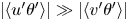 $|\langle u'\theta '\rangle |\gg |\langle v'\theta '\rangle |$, the angle $\beta$ is far from $0$. Hence, a large $\beta$ is not a big concern downstream of the reattachment, where the flow is very similar to a boundary layer. It is more of a concern in the direct vicinity of the gap. However, there, we see that $\beta$ is small. This suggests that an eddy conductivity assumption is not as bad as the eddy viscosity assumption. It is worth noting that a turbulent Prandtl number-type model would still be a bad assumption because it relies on the eddy viscosity to compute the eddy conductivity, the former of which is negative in the vicinity of the gap.
4. Reynolds-averaged Navier Stokes
The recent literature shows much promise of scale-resolving tools (Reference Lehmkuhl, Park, Bose and MoinLehmkuhl, Park, Bose, & Moin, 2018; Reference Milani, Gunady, Ching, Banko, Elkins and EatonMilani et al., 2019; Reference Romero and GrossRomero & Gross, 2019; Reference Wu and PiomelliWu & Piomelli, 2018; Reference Xia, Kalitzin, Lee, Medic and SharmaXia, Kalitzin, Lee, Medic, & Sharma, 2020; Reference Xu, Yang and MilaniXu, Yang, & Milani, 2021b; Reference Zhao and SandbergZhao & Sandberg, 2021) and machine learning (Reference Milani, Ling and EatonMilani, Ling, & Eaton, 2020; Reference Milani, Ling, Saez-Mischlich, Bodart and EatonMilani, Ling, Saez-Mischlich, Bodart, & Eaton, 2018; Reference Waschkowski, Zhao, Sandberg and KlewickiWaschkowski, Zhao, Sandberg, & Klewicki, 2021; Reference Weatheritt, Zhao, Sandberg, Mizukami and TanimotoWeatheritt, Zhao, Sandberg, Mizukami, & Tanimoto, 2020; Reference Zhou, He and YangZhou, He, & Yang, 2021). However, RANS is still the workhorse for the fluid engineering. In this context, knowing which RANS model may work for a flow is critical to engineering design. In § 3, the results suggest that the negative eddy viscosity may be a consequence of flow hysteresis. We speculate that Reynolds stress models (RSMs) that account for flow's hysteresis would outperform eddy viscosity-type RANS models that forces the Reynolds stress tensor to align with the local velocity strain rate. In this section, we test this speculation by comparing the RSM (Reference Gibson and LaunderGibson & Launder, 1978; Reference Speziale, Sarkar and GatskiSpeziale, Sarkar, & Gatski, 1991), the  $k$–
$k$– $\omega$ SST model (Reference MenterMenter, 1994) and the DNS.
We employ the commercial software STARCCM+, an extensively used commercial software, for our RANSs. In the following, we briefly summarize the details of our RANS calculations. The RANS domains span from  $x=-6d$ to $x=30.5d$ in the $x$ direction. The $y$ and $z$ dimensions of the domain and the boundary conditions are the same between the RANSs and the DNSs. The RANS grids are the same as their DNS counterparts.
The SST  $k\text {--}\omega$ model is an eddy viscosity-type model and is among the more accurate RANS models when it comes to film cooling applications (Reference Harrison and BogardHarrison & Bogard, 2008). By solving two transport equations for the turbulent kinetic energy $k$ and the specific dissipation rate $\omega$, the SST model does account for the hysteresis in the eddy viscosity. However, because the model relies on the Boussinesq assumption and forces the local Reynolds stress tensor to align with the local velocity strain tensor, it does not account for the hysteresis in the Reynolds stress itself. The model requires the specification of the mean flow, the turbulent kinetic energy, and the eddy viscosity at the inlet. At the inlet, we impose the mean flow and the turbulent kinetic energy from the DNSs. The eddy viscosity is such that it gives DNS’ $\langle u'v'\rangle$. Further details of the SST model and its implementation in STAR-CCM+ can be found in Reference MenterMenter (Reference Menter1994) and Siemens (2020) and are not repeated here for brevity.
Compared with eddy viscosity type models, RSMs are far less often used for film cooling applications. The RSM model solves the transport equations for each Reynolds stress component and therefore directly accounts for the hysteresis in Reynolds stress itself. Nonetheless, writing the transport equations for the Reynolds stresses does not solve the turbulence closure problem. The pressure–strain term, the turbulent diffusion term, and the dissipation term in the Reynolds stress transport equations must be closed. The solver employs the closures in Reference Gibson and LaunderGibson and Launder (Reference Gibson and Launder1978). For a fair comparison, we feed the same inflow information to the RSM as the SST. That is, we provide only the mean flow, the turbulent kinetic energy, and the eddy viscosity at the inlet. The solver solves each Reynolds stress equation as follows:
 \begin{equation} \left.\begin{array}{@{}c@{}} \langle vv\rangle = \dfrac{2}{3}k-2\mu_t\dfrac{{\rm d}V}{{\rm d} y}, \\ \langle ww\rangle = \dfrac{2}{3}k-2\mu_t\dfrac{{\rm d}W}{{\rm d}z} = \dfrac{2}{3}k, \\ \langle uu\rangle = 2k-\langle vv\rangle -\langle ww\rangle , \\ \langle uv\rangle = {-}\mu_t\dfrac{{\rm d}U}{{\rm d} y}. \end{array}\right\} \end{equation}
Note that the above is the implied Reynolds stresses in the SST model but does not necessarily match the DNS. The reader is directed to Reference Gibson and LaunderGibson and Launder (Reference Gibson and Launder1978) and Siemens (2020) for further details of the model.
As for heat transfer, both the SST and the RSM solve the heat flux  $q$ according to
 \begin{equation} q = {-}\left(\lambda + \frac{\mu_t C_p}{Pr_t}\right)\boldsymbol{\nabla} T. \end{equation}
The eddy viscosity is readily defined in the SST model. For the RSM, the eddy viscosity is redefined according to
 \begin{equation} \mu_t = \rho C_\mu k T_t, \end{equation}
where  $C_\mu$ is a model coefficient, $k$ (again) is the turbulent kinetic energy and $T_t$ is a turbulent time scale. Again, details of the model coefficients can be found in Siemens (2020) and are not repeated here for brevity.
Next, we show the results. Figure 17 shows the cooling effectiveness and the skin friction coefficient for all cases. Now, expecting a RANS model to accurately capture flow separation without any calibration is unrealistic. Nonetheless, we see that the RSM clearly outperforms the SST model, thereby confirming our speculation about flow hysteresis. A more in-depth discussion of the RANS results falls outside of the scope of this work and will be left for future investigation. Nonetheless, it is worth noting that point-by-point local comparison of the RSM predicted Reynolds stress with DNS is not very useful and would not give much insight into flow hysteresis.
Skin friction coefficient in (a) FWD-M5, (c) FWD-M2, (e) FLT-M5, (g) FLT-M2, (i) BWD-M5, (k) BWD-M2. Cooling effectiveness in (b) FWD-M5, (d) FWD-M2, ( f) FLT-M5, (h) FLT-M2, (j) BWD-M5, (l) BWD-M2.

5. Conclusions
This paper reports DNS results of leakage flow downstream of a forward misalignment configuration, an aligned configuration and a backward misalignment configuration for the blowing ratios  $M=0.2$ and 0.5. The higher blowing ratio, i.e. $M=0.5$, lifts the leakage jet higher above the downstream plate's surface and gives rise to a larger separation bubble than the lower blowing ratio, i.e. $M=0.2$. Meanwhile, the higher blowing ratio, i.e. $M=0.5$, brings more cold fluid into the domain and leads to a cooler plate far downstream than the lower blowing ratio. Comparing the three misalignment configurations, the forward misalignment pushes the leakage jet higher above the wall, leading to a decreased cooling effectiveness compared with the aligned configuration, and the backward misalignment pushes the leakage jet towards the wall, leading to increased cooling effectiveness. Two mixing layers emerge. The windward mixing layer stays laminar for a longer distance than the leeward mixing layer, the latter of which rapidly mixes with the surrounding flow and is responsible for a lot of the turbulence generation in the flow. The windward mixing layer is responsible for most heat exchange between the cold leakage jet and the surrounding hot fluid. The validity of Boussinesq's hypothesis is assessed for both eddy viscosity and eddy conductivity. The data show that Boussinesq's eddy viscosity hypothesis is not valid within the regions where the leakage jet begins to mix with the surrounding flow. Analysis shows that flow hysteresis and a small mean flow time scale are responsible for the failure of Boussinesq's eddy viscosity hypothesis in these regions. Although the eddy conductivity is a poor hypothesis, its failure is mainly because of well-correlated streamwise velocity and temperature fluctuations. The analysis shows that, if a high-fidelity scale-resolving tool is not available, RSMs, which account for flow hysteresis, will give more accurate results than eddy viscosity type models, which assume local equilibrium between the mean flow and the underlying turbulence.
Acknowledgements
The DNSs were performed on ACI-ICS at Penn State.
Declaration of Interests
The authors report no conflict of interest.
Funding Statement
This research received no specific grant from any funding agency, commercial or not-for-profit sectors.
Data Availability Statement
Raw data are available from the corresponding author.
Appendix A. Further analysis of the eddy viscosity and the eddy conductivity
The Boussinesq assumption concerns both the magnitude and the alignment. The main text examines the eddy viscosity magnitude and the misalignment between the modelled and the real heat flux. This appendix further examines the (mis)alignment between the modelled and real Reynolds stress. We will also show the eddy conductivity magnitude.
The full eddy viscosity assumption concerns both the diagonal and off-diagonal components and reads
 \begin{equation} b_{ij} = {-}2\nu_tS_{ij}, \end{equation}
where  $b_{ij}=R_{ij}-R_{kk}\delta _{ij}/3$ is the anisotropic part of the Reynolds stress tensor, and $S_{ij}$ is the velocity strain rate tensor. The indices $i$ and $j$ is 1 or 2 as the mean flow is two-dimensional. Both $b_{ij}$ and $S_{ij}$ are zero-trace symmetric tensor and therefore can be written as
 \begin{equation} {\boldsymbol b} = {\boldsymbol v}_1'{\boldsymbol{\varLambda}_1}{\boldsymbol v}_1, \quad {\boldsymbol S} = {\boldsymbol v}_2'{\boldsymbol{\varLambda}_2}{\boldsymbol v}_2, \end{equation}
where  ${\boldsymbol v}_{1,2}$ is the eigenvector matrix, ${\boldsymbol \varLambda }_{1,2}$ is the eigenvalue matrix and the superscript $\prime$ denotes transpose. Because both ${\boldsymbol b}$ and ${\boldsymbol S}$ are traceless, their eigenvalue matrices must be
 \begin{equation} \boldsymbol{\varLambda}_{1,2}\sim \begin{bmatrix} 1 & 0 \\ 0 & -1 \end{bmatrix}. \end{equation}
Meanwhile, because both  ${\boldsymbol b}$ and ${\boldsymbol S}$ are symmetric, their eigenvectors are orthogonal and ${\boldsymbol v}_{1,2}$ is a unitary matrix. It follows that the validity of the Boussinesq eddy viscosity assumption relies on whether the eigenvectors of ${\boldsymbol b}$ and ${\boldsymbol S}$ align, and deviations from the Boussinesq eddy viscosity assumption may be measured by the angle between ${\boldsymbol b}$ and ${\boldsymbol S}$ eigenvectors, as sketched in figure 18. Figure 19 shows the angle $\alpha$ between ${\boldsymbol b}$ and ${\boldsymbol S}$ eigenvectors. We see that the Boussinesq eddy viscosity is a poor approximation in the windward mixing layer as well as the region near the leading edge of the downstream plate. This is consistent with figure 14. Compared with the cases with a lower blowing ratio, i.e. $M=0.2$, the higher blow ratio, i.e. $M=5$, results in a more lifted leakage jet, which, in turn, gives rise to a larger area within which $\alpha$ is large. The plate misalignment has a notable impact on $\alpha$ values in the cases with a lower blowing ratio: deviations from the Boussinesq eddy viscosity assumption is less significant in the BWD configuration than the FWD configuration. This is, again, consistent with figure 14.
A sketch of how one can measure deviations from the Boussinesq eddy viscosity assumption. Here, blue arrows indicate eigenvectors of  ${\boldsymbol b}$, i.e. columns of ${\boldsymbol v}_1$, and red arrows indicate eigenvectors of ${\boldsymbol S}$, i.e. columns of ${\boldsymbol v}_2$. Both ${\boldsymbol v}_{1}$ and ${\boldsymbol v}_2$ are unitary matrix and therefore the arrows are of unit length. We use $\alpha$ to denote the angle between ${\boldsymbol b}$ eigenvectors and ${\boldsymbol S}$ eigenvectors.

The angle between the eigenvectors of  ${\boldsymbol b}$ and ${\boldsymbol S}$ (a) FWD-M5, (b) FWD-M2, (c) FLT-M5, (d) FLT-M2, (e) BWD-M5 and ( f) BWD-M2. The three thin solid black lines are streamlines. The colour bar range is between $-\pi$ and $\pi$. We blank out the laminar region where the turbulent kinetic energy is essentially 0.

The full Boussinesq eddy conductivity is shown in (3.3). The scalar  $\alpha _t$ that best fit the modelled and the real heat fluxes is
 \begin{equation} \alpha_t = {-}\frac{\langle u\theta\rangle \dfrac{{\rm d}\theta}{{\rm d}\kern0.7pt x} + \langle v\theta\rangle \dfrac{{\rm d}\theta}{{\rm d} y}}{\left(\dfrac{{\rm d}\theta}{{\rm d}\kern0.7pt x}\right)^2 + \left(\dfrac{{\rm d}\theta}{{\rm d} y}\right)^2}. \end{equation}
Figure 20 shows the turbulent eddy conductivity computed according to (A4). Except for regions within which the heat flux is essentially zero, i.e. upstream of the windward mixing layer and a small region at the bottom of the recirculation bubble, we see that the eddy conductivity exists everywhere – this is why we resort to a more stringent assessment in the main text. Nonetheless, the results in figure 20 are still interesting to look at. We see that the higher blow ratio  $M=0.5$ gives rise to a region of high eddy conductivity in the rear part of the recirculation bubble; such a region cannot be found in the lower blowing ratio cases. The misalignment configuration impacts the lower blowing ratio $M=0.2$ cases more than the higher blowing ratio $M=0.5$ cases. Specifically, the forward misalignment leads to higher eddy conductivity after the flow re-attaches than the FLT configuration, and the FLT configuration than the BWD configuration.
Eddy conductivity computed according to (A4) in (a) FWD-M5, (b) FWD-M2, (c) FLT-M5, (d) FLT-M2, (e) BWD-M5, and ( f) BWD-M2. The three thin solid black lines are streamlines. We blank out regions with which the turbulent heat flux is essentially 0.

Appendix B. Grid convergence of RANS
In this appendix, we present a grid convergence study for our RANS. We double the grid resolution in both  $x$ and $y$ directions for case FWD-M5, i.e. the case with the most vigorous turbulence. Figure 21 shows the RANS predicted skin friction and cooling effectiveness. We see that the results collapse, confirming grid convergence of our RANSs.
RANS results for FWD-M5. (a) Skin friction coefficient; (b) cooling effectiveness. We double the DNS grid resolution in both  $x$ and $y$ directions, and the fine grid RANSs are denoted using ‘fine’.


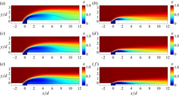


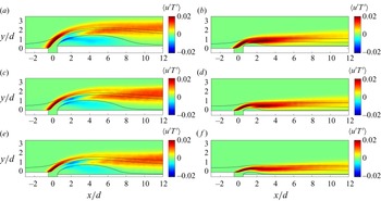


 Open access