


1. Introduction
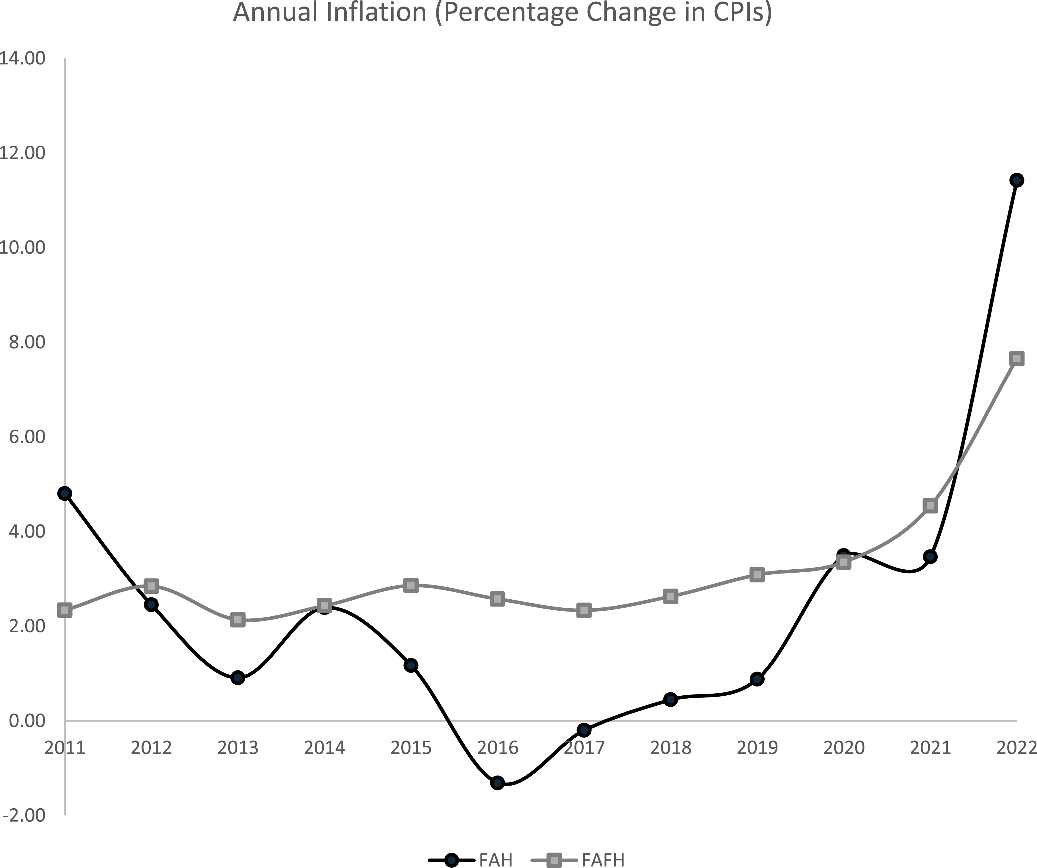
Two related events over the last several years have significantly impacted food prices. First, the COVID-19 pandemic affected both the demand and supply of goods, inducing negative effects on the economy, especially in the food sector. Second, during and after the pandemic, a combination of expansionary policies and economic factors led to food price inflation with differential effects in the food-at-home (FAH) and food-away-from-home (FAFH) prices. In the five years before the pandemic (2015–2019), the average annual inflation rates of the consumer price indexes (CPI) for FAH and FAFH were 1.28 and 2.58, respectively (Figure 1). However, for 2020, 2021, and 2022, the corresponding inflation rates were 3.35, 4.54, and 7.66 for FAFH and 3.49, 3.46, and 11.42 for FAH, with 2022 representing the highest in 40 years.
Annual CPIs of FAH and FAFH between 2010-2022.
Sources: Authors’ calculations based US Department of Labor Bureau of Labor Statistics (2023b).
Notes: FAH = food at home; FAFH = food away from home.
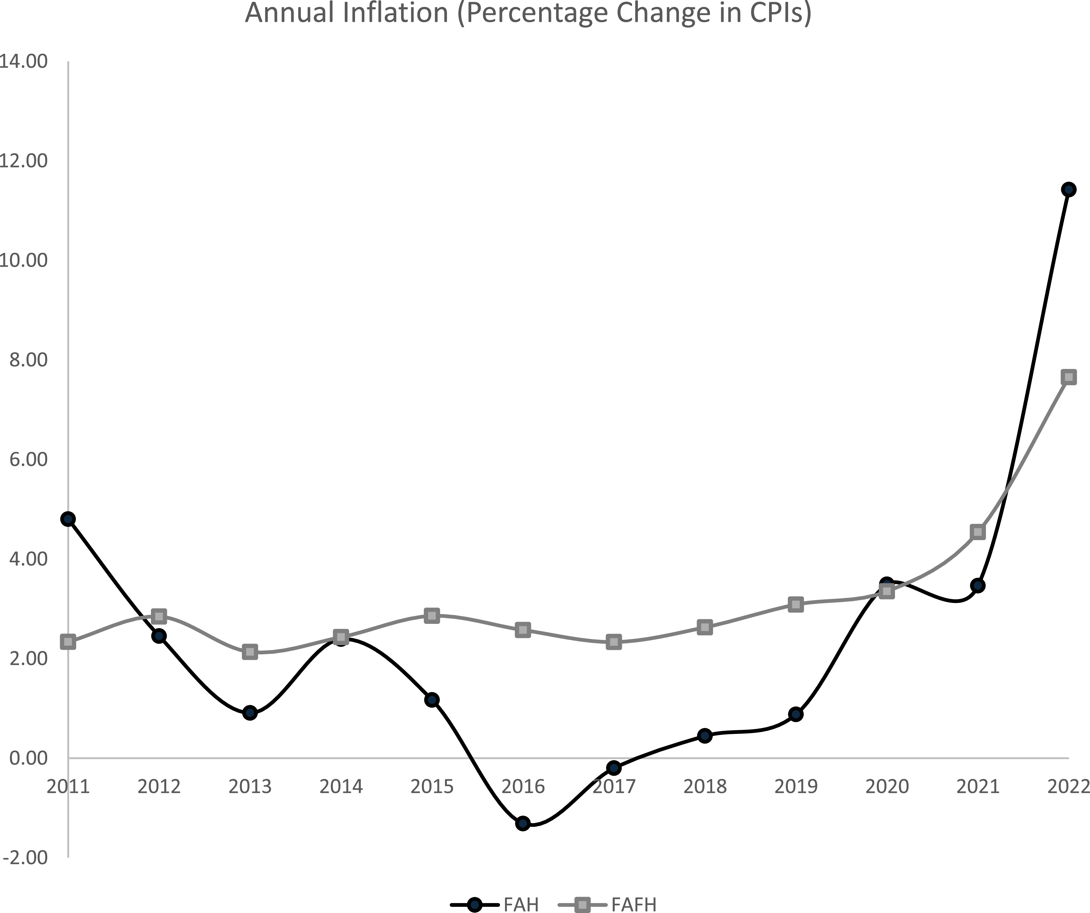
While food price inflation has been, and continues to be, a major topic in the popular press (e.g., Stamm and Newman Reference Stamm and Newman2024; Thomas Reference Thomas2025), political circles (e.g., Fair Grocery Pricing Act H.R. 1788, 2025-2026; Reduce Food Prices Act H.R. 701, 2025-2026), and in the academic literature (e.g., Adjemian et al. Reference Adjemian, Arita, Meyer and Salin2024; Blanchard and Bernanke Reference Blanchard and Bernanke2023; Parum and Dharmasena Reference Parum and Dharmasena2024), our paper investigates a fundamental question not yet addressed in the literature: what has been the effect of the changing prices of FAH and FAFH on consumer welfare? The main implication of our findings is not specific to the COVID-19 period or its immediate aftermath but rather explores the more fundamental, and unexplored, issue that the welfare effects of price shocks to FAH and FAFH can be quite different and therefore the implications and appropriate considerations for policy analyses and recommendations could be in turn be quite different.
Answering this question requires analyzing both own- and cross-price effects on other goods (categories) from changing FAH and FAFH prices. The standard approach to estimating own- and cross-price effects for food is by either focusing on disaggregated foods within conditional demand systems without including other aggregates or grouping FAH and FAFH under the broad category of food, thus not allowing for differential impacts. In the conditional demand systems, perhaps not surprisingly due to data and method differences, the existing literature does not provide a consensus on elasticity measures even in ordinal categorization of inelastic and elastic.
For example, Okrent and Alston (Reference Okrent and Alston2011) find FAH and FAFH own-price elasticities of −0.48 and −1.02, respectively, whereas Lusk (Reference Lusk2017) finds FAH and FAFH elasticities of −1.07 and FAFH at −1.16, respectively. Lusk (Reference Lusk2017) and Okrent and Kumcu (Reference Okrent and Kumcu2016) adopted a disaggregated conditional approach, partitioning foods based on the degree of preparation. These investigations were primarily aimed at estimating disaggregated systems for food groups, including cereals, dairy, fruits, vegetables, and meats, similar to Okrent and Alston (Reference Okrent and Alston2012). A common finding across all these papers is that the food categories that offer more convenience like FAFH have higher own price elasticities than those that are less convenient like FAH (e.g., Davis Reference Davis2014; Lusk Reference Lusk2017; Okrent and Alston Reference Okrent and Alston2011).
However, basic utility maximization-demand system analysis indicates that changing food prices in theory can not only affect food spending, but also spending on other non-food items (e.g., Deaton and Muellbauer Reference Deaton and Muellbauer1980). Boonsaeng and Carpio (Reference Boonsaeng and Carpio2020) estimated a more aggregate demand system with a single food aggregate and other non-food expenditure categories such as utilities, apparel, transportation, medical care, shelter, other nondurables, and durables. They found many statistically significant own- and cross-price effects between food and non-food items, showing complex substitution and complementarity relationships. For example, for the average household (Table C1 in Boonsaeng and Carpio Reference Boonsaeng and Carpio2020) their own-price elasticity estimates implied inelastic household responses for food and other expenditure categories (utilities, apparel and services, transportation, and shelter and household operations), but elastic demands for medical durable and non-durable goods. Similarly, their estimates of 56 cross-price elasticities revealed a complex pattern of significant substitution (30) and complementarity (26) patterns.
Unlike Boonsaeng and Carpio (Reference Boonsaeng and Carpio2020), given the differences in price changes for FAH and FAFH and the potential cross-price effects on non-food expenditures, we are interested in the potential differential effects on FAH, FAFH, and other goods. Such an analysis requires the estimation of a demand system that includes FAH and FAFH along with other broad non-food aggregates. Most importantly, and again in contrast to Boonsaeng and Carpio (Reference Boonsaeng and Carpio2020) and most demand analyses, our focus is on the consumer welfare implications. This will allow us to address three additional secondary questions not yet addressed in the literature:
-
1. How have the changes in prices of FAH and FAFH affected consumer welfare over time?
-
2. Do FAH or FAFH price changes cause greater consumer welfare loss when we consider both own- and cross-price effects across all expenditure categories within the demand system?
-
3. Finally, how do the effects of FAH and FAFH prices on consumer welfare differ during typical periods of stable growth compared to macroeconomic crisis periods?
Our approach addresses two gaps in the existing literature while answering the broader policy questions of interest. First, by estimating the changes in consumer welfare due to own- and cross-price effects of FAH and FAFH prices, we explicitly consider the changing mix of FAH and FAFH consumption. Second, our consideration of other non-food expenditure categories such as rent, utilities, transportation, durables, medical, etc., allows for substitutability and complementarity across all expenditure categories amidst rising FAH and FAFH prices during and after the COVID-19 pandemic.
Addressing these two gaps leads to three contributions to the literature on food demand and welfare analysis. First, we show that the welfare implications of food price inflation depend on the consumption channel through which food is acquired, i.e., whether FAH or FAFH. Despite higher increases in FAFH prices, FAH price increases generate larger and more volatile welfare losses, reflecting differences in price elasticities and budget shares across the two categories. Second, our results show that own-price effects of food price inflation dominate welfare calculations, with cross-price effects across food and non-food categories having a limited negligible impact. Third, we find that during major macroeconomic shocks, like the COVID-19 pandemic, welfare losses are amplified through relatively inelastic consumption categories like FAH. Overall, our paper highlights the importance of distinguishing between FAH and FAFH in both empirical and policy analyses of food price changes.
The rest of the paper is structured as follows. We first provide a background discussion of the structural and behavioral factors that distinguish FAH and FAFH price dynamics and their welfare implications. We then describe how we prepared the data for our analysis and present summary statistics, followed by an outline of the methodology that includes the demand system estimation and welfare loss calculations. The last section provides an expanded discussion and conclusions that situate the findings within the broader literature and draw forward-looking policy implications.
1.1. Background: FAH and FAFH price divergence dynamics
The divergence between FAH and FAFH price dynamics reflects fundamentally different cost structures, production, and supply chains of the two different marketing channels, including consumer behavioral responses to price changes in the food categories. The USDA ERS Food Dollar (Baker and Zachary Reference Baker and Zachary2026) provides a comprehensive supply-chain accounting of exactly where each dollar spent on FAH and FAFH goes. For example, in 2023, of every dollar spent on domestically produced FAH, approximately 28.5 cents went to food retail (e.g., grocery stores), 26.6 cents to food processing, 11.7 cents to food wholesale, 10.6 cents to farm commodities, and 0.3 cents to food services, (other is 17.5 cents).
The FAFH dollar is constituted in a fundamentally different way where food services (e.g., restaurants, prepared items) alone accounted for 67.0 cents of every FAFH dollar spent, while food processing claimed only 7.4 cents, farm commodity 4.2 cents and food retail a mere 2.4 cents (other is 14.7 cents). This structural divergence shows that FAH and FAFH are not simply different consumption categories for the same underlying product but are distinct in different supply chains with different inputs and cost drivers. Consequently, and not surprisingly, price movements throughout the supply chain for these two different final downstream products will be different. Recognizing these structural differences provides the conceptual foundations and motivation for our analysis that separates FAH and FAFH price effects to estimate welfare implications for consumers, which is different from prior analyses that aggregate FAH and FAFH under a single food category.
1.2. Supply-side (structural) factors
FAH and FAFH operate under distinct cost structures and pricing mechanisms because the retail grocery channel and the food-service channel differ substantially in input cost composition. On one hand, FAH prices primarily reflect retail food markets, where goods are purchased for preparation of meals at home, and as such upstream competition in the food supply chain, input costs, and retail markups determine prices (Adjemian et al. Reference Adjemian, Arita, Meyer and Salin2024). On the other hand, FAFH prices embed not only food input costs, but also labor, service, rent, convenience, etc., which make FAFH closer to a bundled service good (e.g., Davis Reference Davis2014; Ellickson Reference Ellickson2016; Rahkovsky et al. Reference Rahkovsky, Jo and Carlson2018). Since FAFH prices are heavily weighted towards these additional factors such as labor, rent, etc., FAFH prices are likely more sensitive to labor shortages, service industry turnover cycles, minimum wage increases, etc. These differences cause FAH and FAFH price volatility to vary to distinct macroeconomic shocks with different speeds and magnitudes. The COVID-19 pandemic illustrates this point. The supply chain disruptions in spiked FAH prices initially, while lockdowns suppressed FAFH demand before labor shortages later drove FAFH prices upwards (Adjemian et al. Reference Adjemian, Arita, Meyer and Salin2024; Blanchard and Bernanke Reference Blanchard and Bernanke2023).
1.3. Demand-side (behavioral) factors
From a demand-side perspective, the two categories differ in terms of convenience, time costs of preparing meals, and consumers treat FAH and FAFH as imperfect substitutes with different underlying preferences. FAH includes staples and necessity food items that typically have lower price elasticity of demand, which means that consumers are unable to exit the market even if grocery prices rise (Lusk Reference Lusk2017; Okrent and Alston Reference Okrent and Alston2011). FAFH, on the other hand, is more price elastic because it is subject to greater substitution toward FAH when relative prices tilt toward FAH. The differential elasticity reflects the time cost of food preparation for FAH, or “full price,” compared to FAFH that saves the time input into meal preparation (Becker Reference Becker1965; Davis Reference Davis2014). So, when away-from-home options are more expensive, some households may substitute their own-time to compensate for market-purchased convenience. The consistently higher own-price elasticities for FAFH relative to FAH is found in the literature to confirm the behavioral pattern (Lusk Reference Lusk2017; Okrent and Alston Reference Okrent and Alston2011; Okrent and Kumcu Reference Okrent and Kumcu2016).
1.4. Distributional welfare implications
The two food categories differ in their role within the broader household budget, making the distributional consequences of price shocks for FAH and FAFH different across different household groups. For example, lower income households allocate a substantial higher budget share to FAH, compared to higher FAFH spending by high-income households (Boonsaeng and Carpio Reference Boonsaeng and Carpio2020). FAH has stronger links with overall food security, whereas FAFH can be more easily adjusted along both intensive and extensive margins (Lin and Guthrie Reference Lin and Guthrie2012). This distinction implies that price changes in FAH are likely to generate first-order welfare effects compared to more second-order effects that include substitution within food and across non-food categories for FAFH price changes. Overall, it is likely that FAH price shocks are likely to be more regressive, disproportionately burdening households with less resources to absorb price increases to substitute for alternative food options. The distributional dimension motivates our focus on consumer welfare, not just demand elasticities, and underscores why it matters whether FAH or FAFH prices rise faster during inflationary episodes. It also guides our empirical analysis, which explicitly allows for differential own- and cross-price effects across FAH, FAFH, and other expenditure categories within a demand system framework.
2. Data
Following the approach of studies like those by Boonsaeng and Carpio (Reference Boonsaeng and Carpio2020) and Okrent and Alston (Reference Okrent and Alston2012), we used data from two sources. For expenditures, we used the publicly accessible Consumer Expenditure Survey (CEX) quarterly interview data from 2006 to 2022 (US Department of Labor Bureau of Labor Statistics [BLS] 2023a). The data consist of aggregate expenditures on nine expenditure categories, including FAH, FAFH, apparel and services, transportation, medical care, shelter and household operations, durable goods, and non-durables.Footnote 1 For price information, we used regional Consumer Price Index (CPI) data (US Department of Labor BLS 2023b) from the Federal Reserve Bank of St. Louis (FRED), which is merged to the CEX based on region.
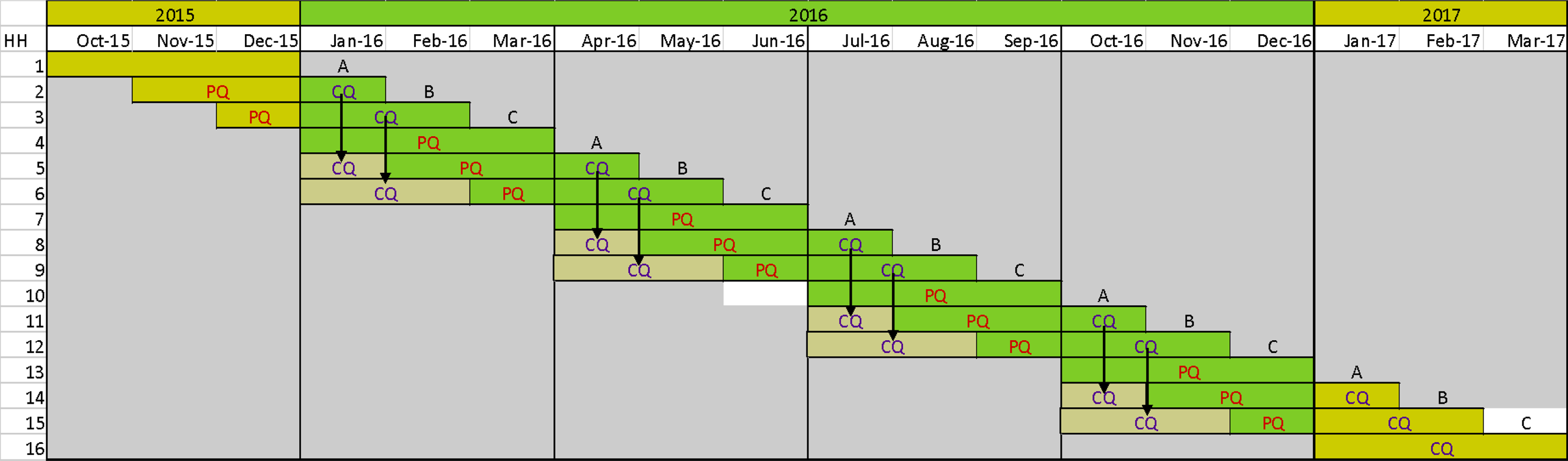
Notwithstanding our different research objectives, like Boonsaeng and Carpio (Reference Boonsaeng and Carpio2020), we conduct an annual analysis but consider an extended time frame from 2006 to 2022 (instead of 2000–2015). The BLS CEX quarterly interview data come from a rotating panel of approximately 7,000 households in each year where the households participate in the survey for five consecutive quarters. Figure 2 gives a visual representation and explanation of how we obtain accurate estimates of annual expenditures of all nine expenditure categories in our analysis for a representative year (2016 for illustration purposes).
Data structure of CEX: Interview survey.
Notes: PQ = Past Quarter, CQ = Current Quarter. A = first panel households, B = second panel households, C = third panel households. Demonstration of how quarterly data were obtained as described in 2001 Consumer Expenditure Survey Interview documentation (p. 259).
Sources: Authors’ rendition based on US Department of Labor Bureau of Labor Statistics (2023a).
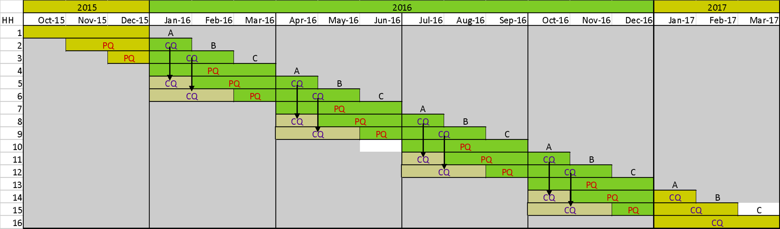
In any given quarter when a representative household reports their expenditure, the CEX survey asks about expenditure in current- or past-quarters (CQ or PQ in Figure 2). For illustration purposes, households can be categorized into three surveyed panels A, B, and C, depending on the month in which they participated in the survey. Households in panels A, B, and C participate in the rotating panel survey in the first, second, and third month, respectively, in a quarter. For example, households in panel A appear in the months of January, April, July, and October in 2016 and January 2017 (see Figure 2).
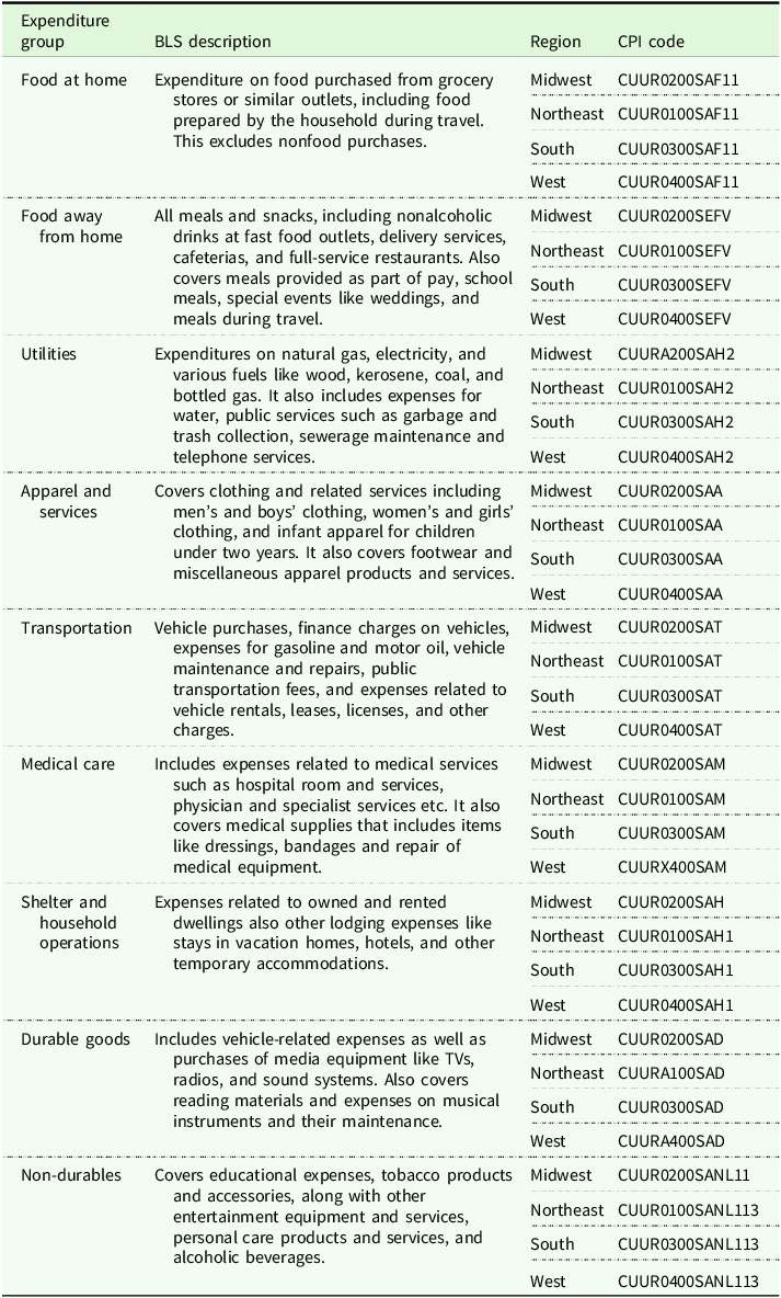
For a household in panel A that starts their interview survey in either January or April of 2016, and fills out five consecutive surveys, we can construct an accurate annual expenditure data for 2016 for that household. However, if a panel A household starts their interview survey in July or October, annual expenditure cannot be constructed due to missing data for the first quarter. Similarly, it is not possible to include panels B and C for the same reason. So, our final annual dataset includes panel A households whose interviews started in either January or April of every year allowing us to avoid missing data and ad hoc imputation problems. The final dataset used in the analysis consists of 5,811 households whose panels were used to construct annual expenditures over the period 2006 to 2022.Footnote 2 Appendix Table A1 provides a detailed description of the various expenditure groups we utilized based on the data obtained by creating a panel of “A” households from FMLY dataset in the interview data. Each group is further described by its specific nature and type of expenditures included, with regional breakdowns (Midwest, Northeast, South, West), and corresponding CPI codes, which are used for tracking changes in consumer prices across different regions (see Appendix Table A1 for detailed description).
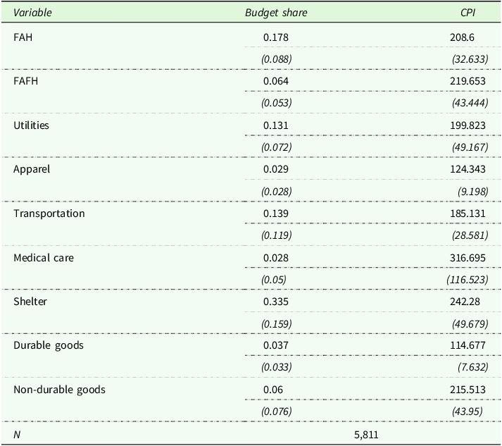
The two columns in Table 1 show the average budget share and CPI for each expenditure category with the respective standard deviations reported in the parentheses. The averages are across all households in the sample from 2006 to 2022 from all regions combined. The budget share represents the proportion of total household expenditure on each category. For example, households on average spent 18% of their total expenditure on FAH compared to 6% on FAFH between 2006–2022. Other major expenditure categories include shelter (34%), transportation (14%), and utilities (13%). Corresponding to the reported budget shares are the average CPI values over the sample period and across all regions for each category with their standard deviations reported in parentheses. The average CPI of FAH is 208.6 and that of FAFH is 219.7.
Summary statistics of budget share and CPI in each expenditure category
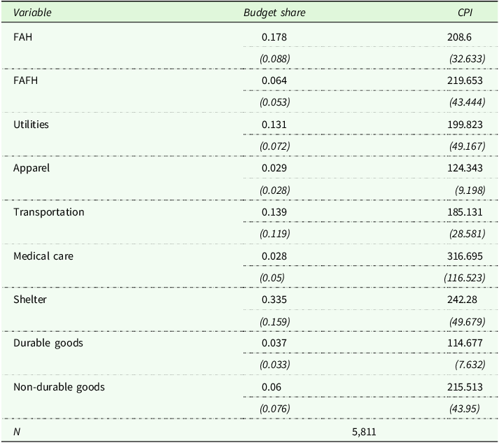
Table 1. Long description
Summary statisctics for 5,811 observations from 2006 to 2022 from all the regions combined. The standard deviations are reported in parentheses. Authors’ calculations based on US Department of Labor Bureau of Labor Statistics Consumer Expenditure Interview Survey public-use microdata (2023a) and Consumer Price Indexes (2023b).
Notes: 5,811 observations from 2006 to 2022 from all the regions combined. The standard deviations are reported in parentheses.
Sources: Authors’ calculations based on US Department of Labor Bureau of Labor Statistics Consumer Expenditure Interview Survey public-use microdata (2023a) and Consumer Price Indexes (2023b).
3. Methodology
To obtain the own- and cross-price effects to be used in the welfare analysis, we estimated the well-known Linear Approximate Almost Ideal Demand System model using Iterative Seemingly Unrelated Regression (ITSUR), imposing homogeneity and symmetry to align with consumer theory. Due to the budget share-based nature of the demand system, excluding one equation is required and enforces the adding-up condition. This study included 8 equations corresponding to the expenditure categories, with the non-durable category derivable from adding up and homogeneity conditions. Following BLS documentation, final survey weights (i.e., FINLWTYY where YY is the year of the survey) are included in the estimation to make the coefficient estimates representative of the U.S. civilian population.
To obtain accurate standard errors, the BLS recommends using a balanced repeated replication (BRR) method that properly accounts for the stratified survey design of the CEX Interview. The CEX Interview data set includes 44 replicate weights (WTREP01 to WTREP44). Each replicate weight was applied to every variable in our demand system, producing 44 sets of weighted variables. We then ran an ITSUR for each set of weighted variables, fitting all 8 equations simultaneously across all expenditure categories in each replicate. This procedure, repeated for all 44 replicates, produced 44 sets of regression coefficients – one set for each replicate-weighted model. Using the 44 replicate sets of regression coefficients and the final weighted regression coefficients, variance was estimated as: $Var\left( {{\beta _{category}}} \right) = {1 \over {44}}\sum _{XX = 01}^{44}{\left( {{\beta _{category,WTREPXX}} - {\beta _{category,FINLWTYY}}} \right)^2}$
where β category, WTREPXX represents the estimated coefficient for a specific category (e.g., FAH) based on the XX th replicate, XX = 1, …, 44, and β category, FINLWTYY is the corresponding estimated coefficient from final weighted coefficient estimates. The standard error was then derived as the square root of this variance, giving us a corrected measure that captures variability across all replicates.
We initially included regional dummy variables and COVID period dummies in the system. The joint F tests for including regional and COVID-19 dummy variables revealed that they were not statistically significant, indicating a national model is suitable for estimating the welfare effects of price changes in FAH and FAFH. The needed Marshallian (uncompensated) elasticities were derived from the model’s parameters using precise approximations from Green and Alston (Reference Green and Alston1990).
3.1. Welfare loss analysis
Loss in consumer surplus (LCS) is based on a linear approximation.Footnote 3 The own-price effects on LCS, or within LCS, resulting from price changes in the FAH and FAFH categories for each k = {FAH, FAFH}, time t and region r is calculated with the following formulas: $LCS_{k,r,t}^k = {\it\Delta} {P_{k,r,t}}Q_{k,r,t}^0\left[ {1 + 0.5\;\left( {{{\Delta {P_{k,r,t}}} \over {P_{k,r,t}^0}}} \right){{\hat \varepsilon }_{k,k}}} \right]$
where ΔP
k, r, t
denotes the year-over-year price changes, $Q_{k,r,t}^0$
the initial quantity,
$Q_{k,r,t}^0$
the initial quantity, $P_{k,r,t}^0$
the initial price, and
$P_{k,r,t}^0$
the initial price, and ${{\hat \varepsilon }_{k,k}}$
the estimated own-price demand elasticity for k.
${{\hat \varepsilon }_{k,k}}$
the estimated own-price demand elasticity for k.
Our model also integrates cross-price effects caused by price changes in FAH and FAFH on the consumer surplus associated with other categories j = 1, 2, …, n - 1. The cross-price effects on LCS due to a price change in k = {FAH, FAFH} on category j ≠ k for each region r and time t is calculated as: $LCS_{k,r,t}^j = 0.5\;\left[ {{{Q_{j,r,t}^0\Delta {P_{k,r,t}}} \over {P_{k,r,t}^0}}{{\hat \varepsilon }_{j,k}}} \right]\left[ {P_{j,r,t}^0 - P_{j,r,t}^y - {1 \over a}P_{j,r,t}^y\left( {Q_{j,r,t}^0 + {{Q_{j,r,t}^0\Delta {P_{k,r,t}}} \over {P_{k,r,t}^0}}{{\hat \varepsilon }_{j,k}}} \right)} \right]$
where $P_{j,r,t}^y$
denotes the price coordinate (vertical) intercept for good j and
$P_{j,r,t}^y$
denotes the price coordinate (vertical) intercept for good j and ${{\hat \varepsilon }_{j,k}}$
the estimated cross-price elasticity of j with respect to k. Finally, the total LCS, which includes both own- and cross-price effects for k = {FAH, FAFH}, is given by:
${{\hat \varepsilon }_{j,k}}$
the estimated cross-price elasticity of j with respect to k. Finally, the total LCS, which includes both own- and cross-price effects for k = {FAH, FAFH}, is given by: $TLC{S_{k,r,t}} = LCS_{k,r,t}^k + {\mathop \sum \nolimits_{j \ne k}^{n - 1}}LCS_{k,r,t}^j$
We compute the LCS for each category using regional averages for prices and quantities. The results are then aggregated to obtain annual LCS values for each category, weighted by the sample size of each region for the specific year. Thus, the LCS can be considered the sum of the household regional LCS averages. We again utilized the BRR method, discussed above, to estimate the standard errors for each LCS value. Specifically, 44 distinct elasticity estimates based on the results from 44 separate ITSUR were then used to compute 44 corresponding LCS values and the BRR formula (1) appropriately redefined.
4. Results
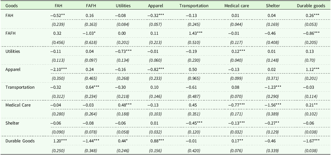
Table 2 gives the estimated own- and cross-price Marshallian elasticities for all categories.Footnote 4 With the exception of transportation, all own-price elasticities are negative and statistically significant at the 90% or higher level. Similar to previous research, the FAH own price elasticity (−0.51) is smaller in absolute value than the FAFH elasticity (−1.03) and more price inelastic than FAFH (e.g., Lusk Reference Lusk2017; Okrent and Alston Reference Okrent and Alston2011). All the expenditure elasticities are positive and significant.Footnote 5 Similar to Boonsaeng and Carpio (Reference Boonsaeng and Carpio2020), we find a complex pattern of substitution (26) and complementarity (29) across all goods. The cross-price elasticities indicate that FAH is a substitute with FAFH, medical care, shelter and durables, whereas it is a complement with utilities, apparel, and transportation, respectively. In contrast, FAFH is a substitute with FAH, apparel, transportation, but a complement with medical care, shelter, and durables goods, respectively.
Estimated Marshallian own- and cross-elasticities for all categories
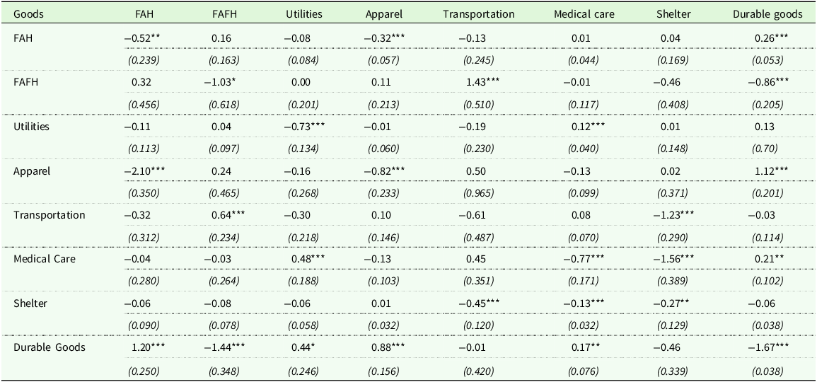
Table 2. Long description
Price elasticities with standard errors in parentheses using balanced repeated replicate (BRR) weights. The sample used is of 5,811 observations per variable from 2006 to 2022 across all regions in the US but it should be remembered within a system context the number of observations is equal to observations per variable times the number of equations (46,488 = 8 x 5,811) . *p<0.10, **p<0.05, ***p<0.010
Notes: Standard errors in parentheses using balanced repeated replicate (BRR) weights. The sample used is of 5,811 observations per variable from 2006 to 2022 across all regions in the US but it should be remembered within a system context the number of observations is equal to observations per variable times the number of equations (46,488 = 8 x 5,811). *p < 0.10, **p < 0.05, ***p < 0.010.
4.1. Welfare loss of changing FAH and FAFH prices
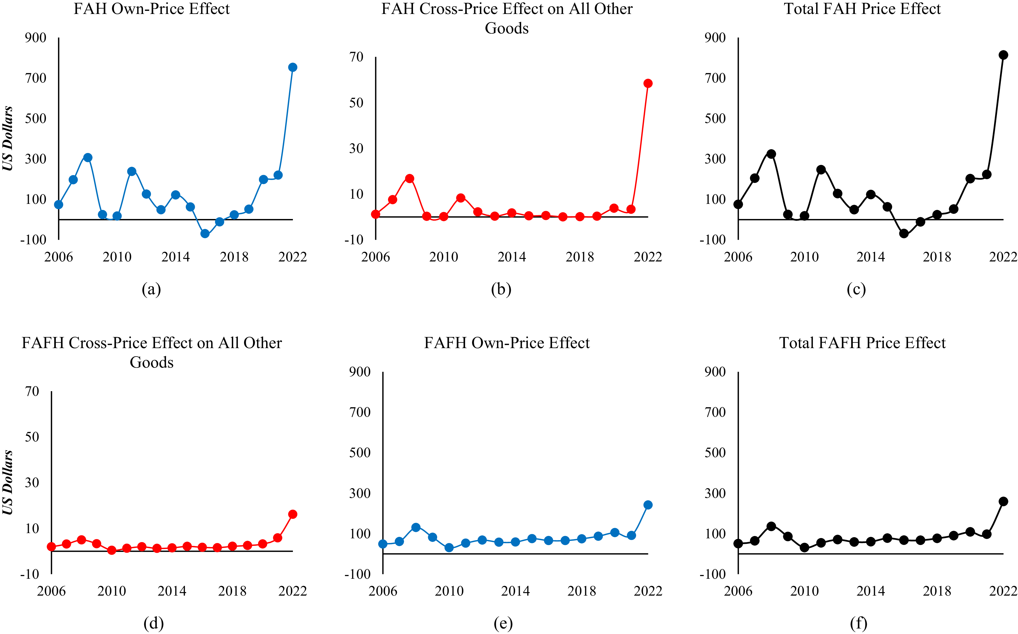
Turning to the main objective of the paper, Figure 3 shows the annual average LCS per household in US dollars at the national level. The first row of panels in Figure 3 capture the LCS from price changes in FAH on FAH (own-price effect) (panel a), on FAFH (cross-price effect) (panel b), and their sum (own- and cross-price effects on FAH and FAFH, respectively) (panel c). The second row captures LCS from price changes in FAFH on FAH (cross-price effect) (panel d), on FAFH (own-price effect) (panel e), and their sum (cross- and own-price effects on FAH and FAFH) (panel f), respectively. Another way of viewing the panels in Figure 3 is the two rows and first two columns make a 2 × 2 matrix with the diagonal panels showing the own-price effects (of FAH and FAFH) and the off-diagonal panels showing the cross-price effects. The third column simply presents the sum of the first two columns, the own- and cross-price effects.
Loss in food only consumer surplus due to price changes in FAH and FAFH.
Notes: The top (bottom) row of panels corresponds to welfare changes due to food at home (FAH) (food away from home [FAFH]) price changes. Panels (a), (b), and (c), respectively show the own-, cross-, and total food loss in consumer surplus (in US dollars) due to FAH price change. Panels (d), (e), and (f) show the cross-, own-, and total loss in consumer surplus due to FAFH price change. Sources: Authors’ calculations based on US Department of Labor Bureau of Labor Statistics Consumer Expenditure Interview Survey public-use microdata (2023a) and Consumer Price Indexes (2023b).
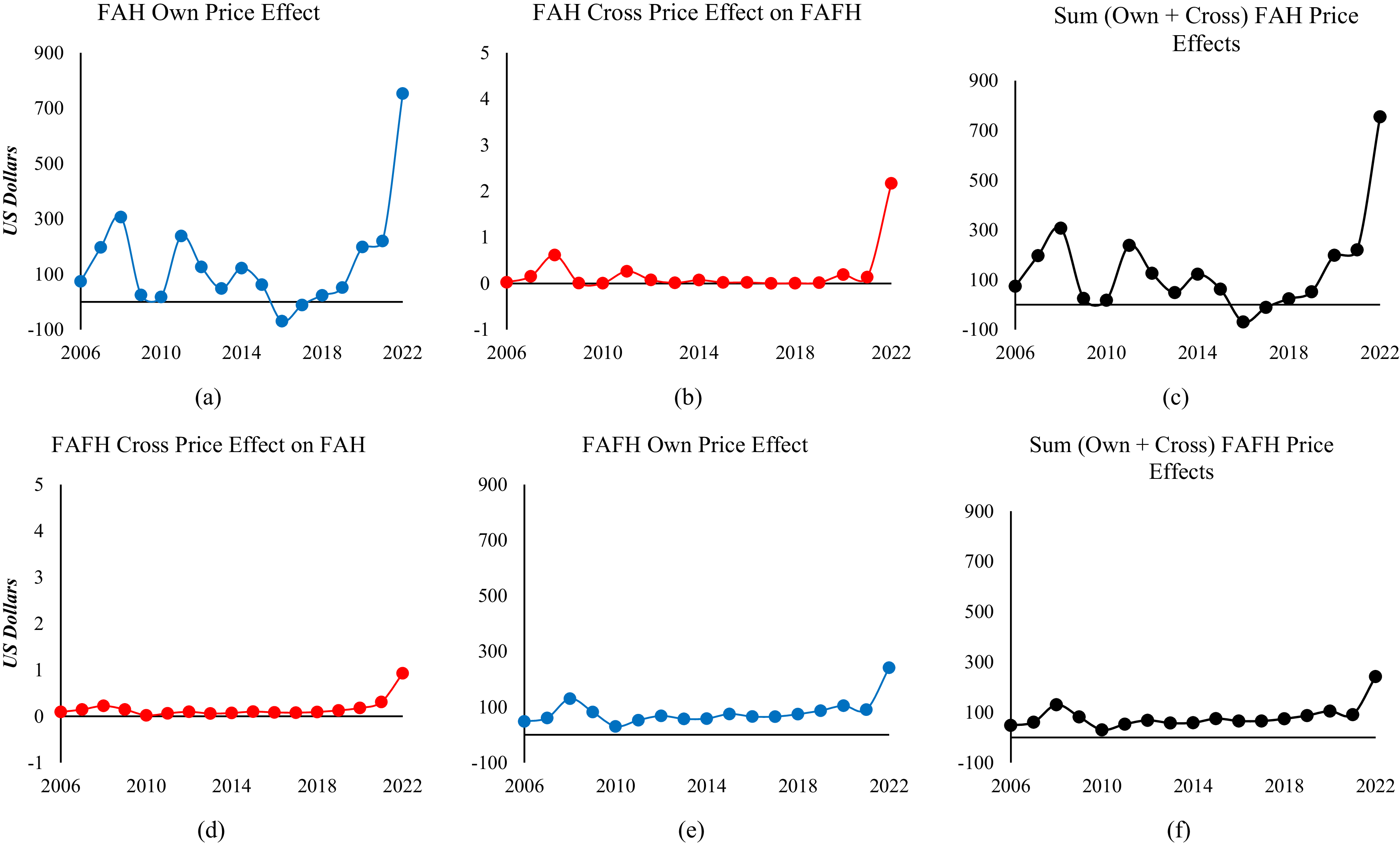
Figure 3. Long description
A six panel figure showing Loss in Food Only Consumer Surplus due tho price changes in Food at home (FAH) and Food Away From Home (FAFH). The top (bottom) row of panels corresponds to welfare changes due to food at home (FAH) (food away from home [FAFH]) price changes. Panels (a), (b), and (c), respectively show the own-, cross-, and total food loss in consumer surplus (in US dollars) due to FAH price change. Panels (d), (e), and (f) show the cross-, own-, and total loss in consumer surplus due to FAFH price change. Authors’ calculations based on US Department of Labor Bureau of Labor Statistics Consumer Expenditure Interview Survey public-use microdata (2023a) and Consumer Price Indexes (2023b).
Regarding the first row, the LCS associated with FAH own-price effect (panel a) ranges from −$70 in 2016 to $700 in 2022. The cross-price effect of FAH on FAFH in terms of LCS is inconsequential (panel b) and the sum across FAH and FAFH (panel c) is effectively equivalent to the FAH own-price effect (panel a). Regarding the second row, there is no consequential cross-price effect of FAFH on FAH (panel d), with the main effect being the own-price effect on FAFH in panel (e), ranging from a low of $30 in 2010 to a high of $241 in 2022. Similarly to the first row, the sum across FAH and FAFH in panel (f) is effectively equivalent to the own FAFH price effect in panel (e). Note in contrast to the first row, the FAFH price effect (in second row) is much less volatile than the FAH price.
Looking across the rows, the LCS findings are consistent with the intuition for consumer surplus associated with our estimated elasticities: FAH is more price inelastic than FAFH and cross price elasticities are inelastic and small. There are three main implications from the results presented in Figure 3.
First, since FAH is comprised of staple food categories with lower price elasticity of demand (Lusk Reference Lusk2017; Okrent and Alston Reference Okrent and Alston2011), consumers face limited substitution options when grocery prices increase. Thus, even a moderate price increase in FAH produces a larger consumer welfare loss than a comparable increase in FAFH prices, because quantity demanded (of FAH) does not fall substantially because FAH demand is inelastic. This means that the full burden of the price increase of FAH is absorbed by the consumer with little substitutability.Footnote 6 This makes LCS in FAH more responsive to its price changes over time. Second, is the magnitude of the loss. The monetary value of consumer welfare loss from FAH is greater when its price changes, affecting both FAH and total loss in welfare from food more significantly than similar changes in FAFH prices. Third, during economic crises like COVID-19, both FAH and FAFH prices increased. However, the consumer welfare impact of FAH price increases was more severe than the FAFH price increases. This is evident from the trends in LCS during 2021 and 2022 compared to the smaller movements seen around the 2008 and 2009 recession, highlighting the unique nature of each crisis. This is consistent with what may be expected as lockdowns during COVD-19 placed more restrictions on FAFH purchases than FAH purchases and thus welfare loss would be more sensitive to FAH price changes than FAFH price changes.
Figure 4 is similar to Figure 3 but is expanded to include the cross-price effects of FAH and FAFH on all other goods, including all seven other non-food expenditure categories in the second and third columns of panels. So, while the diagonal panels of the 2 × 2 matrix of panels (i.e., a and e) in Figure 4 are the same as in Figure 3 (FAH and FAFH own-price effects), the off-diagonal panels now include the cross-price effects of Fah and FAFH on all other expenditure categories, including FAFH and seven others in the case of FAH price change (panel b). With respect to a change in FAFH price, the effect on FAH and the remaining seven categories is given in panel d. The last column of panels, (c and f), represent the total (sum of own- and cross-price on all other categories) effects.
Loss in total consumer surplus due to price changes in FAH and FAFH.
Notes: The top (bottom) row of panels correspond to total welfare changes due to food at home (FAH) (food away from home [FAFH]) price changes. Panels (a), (b), and (c), respectively show the own-, cross-, and total-loss in consumer surplus (in US dollars) due to FAH price change. Panels (d), (e), and (f) show the cross-, own-, and total loss due to FAFH price change. Cross-price includes all categories except FAH (FAFH) in the top (bottom) row.
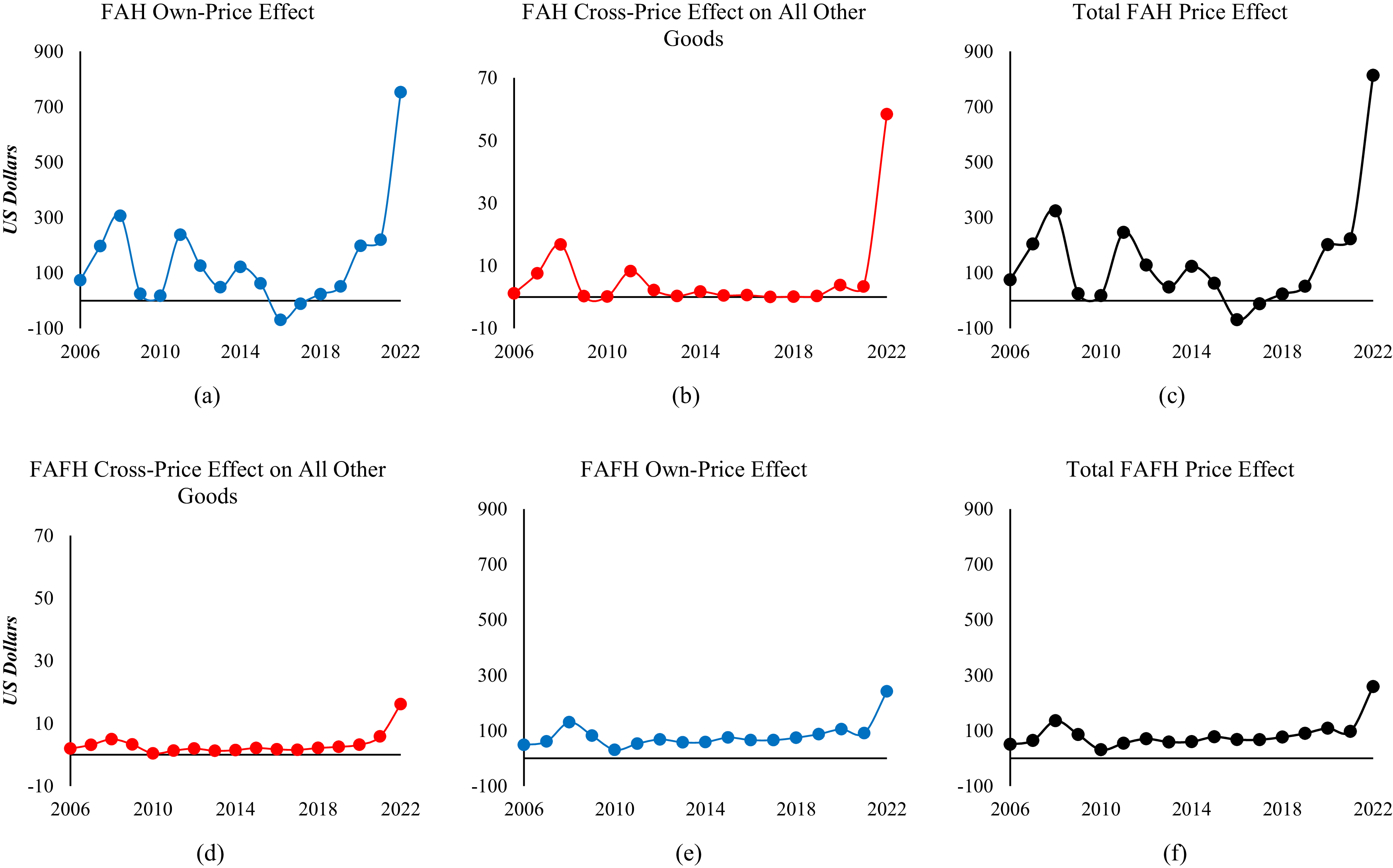
Figure 4. Long description
A six panel figure showing Loss in Total Consumer Surplus due tho price changes in Food at home (FAH) and Food Away From Home (FAFH). The top (bottom) row of panels corresponds to welfare changes due to food at home (FAH) (food away from home [FAFH]) price changes. Panels (a), (b), and (c), respectively show the own-, cross-, and total food loss in consumer surplus (in US dollars) due to FAH price change. Panels (d), (e), and (f) show the cross-, own-, and total loss in consumer surplus due to FAFH price change. Cross-price includes all categories except FAH (FAFH) in top (bottom) row.
The main takeaways from Figures 3 and 4 are the following. The results are comparable in magnitudes and trends when we exclude other non-food expenditure categories (Figure 3) or include them (Figure 4). The total LCS for both FAH and FAFH is still primarily driven by the own-price effects of FAH and FAFH, shown in panels a and e, respectively, in Figures 3 and 4. When the price of FAH increases, it mostly affects its own LCS (panel a), with minimal impact on all other goods (panel b). Similarly, the price increase in FAFH mainly affects its own LCS (panel e), with negligible effects on all other goods (panel d). Thus, the total price effects on LCS (panels c and f) are effectively just determined by the own-price effects.
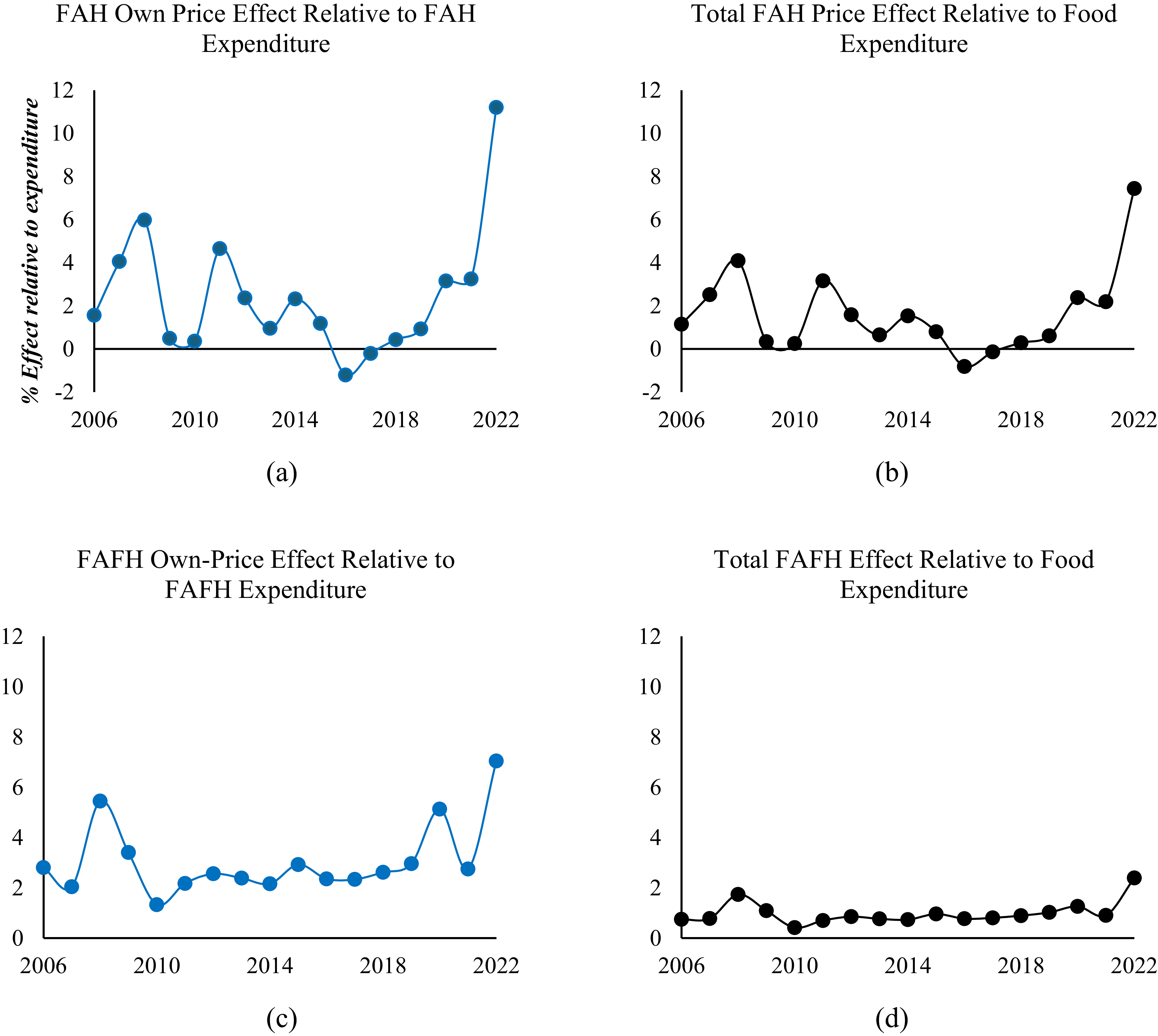
An obvious limitation in interpretation of Figures 3 and 4 is that the two figures are just expressed in absolute dollar amounts, so we have no idea how large these losses are relative to FAH, FAFH, and total food expenditures. So, in Figure 5, we express the own-price effects of welfare losses on FAH (panel a) and FAFH (panel c) relative to their respective expenditures, and the sum of own- and cross-price effects of welfare losses relative to total food expenditures for FAH (panel b) and FAFH (panel d), respectively. The four panels in Figure 5 allow us to express the LCS loss as a percentage of FAH, FAFH, and total food expenditures due to price increases in FAH or FAFH.
Loss in consumer surplus relative to expenditure in each category and total food expenditures.
Notes: The top (bottom) row of panels correspond to welfare changes due to food at home (FAH) (food away from home [FAFH]) price changes. Panels (a), and (b), respectively show negative welfare effects, i.e., loss in consumer surplus (in US dollars) relative to expenditures on FAH and total food due to FAH price change. Panels (c) and (d) show the same for FAFH price change.
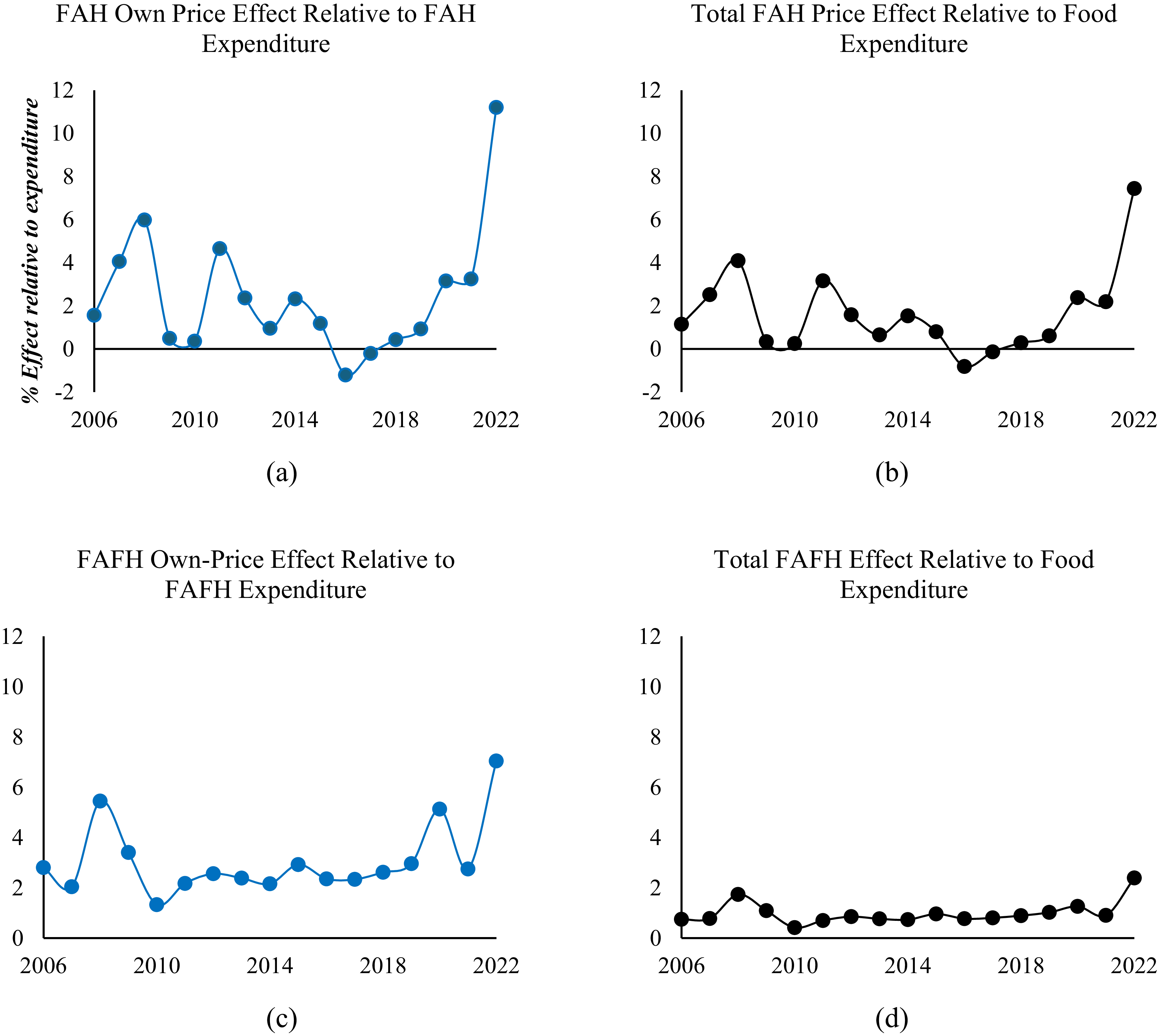
Figure 5. Long description
A four panel figure showing Loss in Consumer Surplus relative to expenditure in each category and total food expenditures. The top (bottom) row of panels correspond to welfare changes due to food at home (FAH) (food away from home [FAFH]) price changes. Panels (a), and (b), respectively show negative welfare effects, i.e., loss in consumer surplus (in US dollars) relative to expenditures on FAH and total food due to FAH price change. Panels (c) and (d) show the same for FAFH price change.
The four panels in Figure 5 provide three key intuitive findings as they relate to consumer welfare loss from FAH and FAFH price inflation. First, similar to absolute changes in LCS, the change in LCS as a percentage of expenditure shows higher variability for FAH compared to FAFH (see panels a and c). We find that relative to their respective expenditures, the percentage LCS from the FAH price changes range between −1.2% to 11.2% between 2006 to 2022, whereas the percentage LCS from FAFH price changes have a lower range of variability between 1.3% to 7%. Second, while the same pattern, i.e., higher percentage losses happened to both FAH and FAFH relative to their expenditures after the Great Recession and the COVID-19 pandemic, the effects were larger for FAH compared to FAFH. During the Great Recession, LCS as a percentage of expenditure was 6% for FAH and 5.4% for FAFH, respectively (see the year 2008 in panels a and c of Figure 5). The difference is larger one year after the COVID-19 pandemic: 11.2% for FAH compared to 7% for FAFH (see year 2022). Finally, the percentage of LCS relative to total food expenditures due to FAH price changes is more variable than the LCS due to FAFH price increase (panels b and d in Figure 5). In case of FAH, it varies between −0.8% to 7.4% whereas in the case of FAFH, the percentage loss varies between 0.4% to 2.4%, respectively.
5. Discussion and conclusions
Utilizing a demand system framework that includes FAH and FAFH along with other broad non-food aggregates, we focus on estimating the consumer welfare effects of FAH and FAFH price changes between 2006–2022, a period spanning two major macroeconomic shocks: The Great Recession and the COVID-19 pandemic with its inflationary aftereffects. The study makes contributions that extend existing research in several directions, with implications that reach well beyond the COVID-19 context.
First, our main finding is that FAH price increases generate larger and more volatile losses in consumer welfare compared to similar FAFH price increases. FAFH prices increased more in absolute terms than FAH prices during 2020–2022 (Figure 1), yet welfare losses were greater (about 11.2%) as a share of total food expenditures from FAH compared to 7% for FAFH, respectively. While surprising, this mechanism follows directly from the theory of consumer demand because FAH is more price inelastic with a higher share of food budget compared to FAFH, consumers cannot readily substitute away from FAH when grocery prices increase, and a larger burden of FAH price increase is absorbed by the consumers than being diffused through behavioral substitution. This finding has a direct implication for policy and discourse on how food price inflation is measured and communicated. While media and other public dialogue treat FAH and FAFH price inflation equivalently or just focus solely on which inflation of the two grew faster, academic and policy discussions should consider the unequal welfare implications of the price inflation of the two food categories for consumers.
Second, we find that own-price effects of FAH and FAFH inflation dominate the impact on consumer welfare with minimal and negligible cross-price effects. This finding has an important methodological implication for the demand literature. Specifically, conditional demand systems with only food sub-categories may be sufficient for welfare analysis of food price shocks, without the added data requirements, modeling, and identification complexities of a full unconditional system. If welfare conclusions of food price inflation are correct without the inclusion of non-food expenditure categories, as our results suggest, then the richer conditional food demand literature (Lusk Reference Lusk2017; Okrent and Alston Reference Okrent and Alston2012; Okrent and Kumcu Reference Okrent and Kumcu2016) can be directly utilized for welfare analysis than previously appreciated. The practical implication is that researchers and policy analysts may not need to wait for the availability of comprehensive expenditure panel data to draw welfare conclusions from food price inflation. Future research could investigate whether this robustness holds in other demand systems (e.g., QUAIDS, EASI, etc.) and/or for other commodity-specific shocks where cross-effects may be more pronounced.
Third, beyond the COVID-19 context, our findings point to a recurring and forward-looking policy challenge: How should policymakers prioritize interventions when food prices spike because of whatever global or domestic macroeconomic shocks? Our results indicate that the appropriate discussion is not the prices of which food category increased faster, but instead which food category consumers are less able to substitute away from. Grocery price stabilization through policies such as investments in resilience of food supply chain, increased retail competition, trade policy adjustments, etc. can have larger welfare effects for consumer than equivalent efforts toward the food service sector. This distinction could inform legislative discussions such as the Fair Grocery Pricing Act (H.R. 1788, 2025–2026) and the Reduce Food Prices Act (H.R. 701, 2025–2026), which specifically target retail grocery prices. Our work is an empirical contribution that supports targeting the policies towards FAH and FAFH price inflations separately because it is not simply a matter of disaggregation, but it reflects the underlying differences in supply- and demand-side factors as outlined in the background. More broadly, our framework that accounts FAH and FAFH own- and cross-price welfare effects separately is applicable to any future food price shock, whether driven by climate disruptions, geopolitical conflicts, or other macroeconomic inflation, and it is independent of the COVID-19 episode for its validity.
Finally, there are several limitations of this analysis that suggest possible opportunities for future research. We conduct an aggregate level study using broad expenditure categories. Disaggregating FAH and FAFH into sub-categories such as by food type, degree of processing, etc. could identify heterogeneity in welfare impacts across product types. By considering a demand framework that allows for interaction with, or sub-analysis by, demographic variables can provide insights into the distributional consequences of price inflation of the two food categories, given than low-income households allocate a substantially higher share of their food budget to FAH (Boonsaeng and Carpio Reference Boonsaeng and Carpio2020). Our aggregate framework cannot fully characterize these distributional effects across income, time constraints, and access to food markets, but the finding that FAH welfare losses dominate FAFH provides a strong prior that heterogeneity analysis deserves attention in future work. These extensions would further strengthen the generalizability of the differential welfare analysis conducted in this paper.
Supplementary material
The supplementary material for this article can be found at https://doi.org/10.1017/age.2026.10031.
Data availability statement
The data that support the findings of this study were (are) publicly available data found at the Bureau of Labor Statistics as given in the references.
Funding statement
Supported by USDA National Institute of Food and Agriculture Grant 2023-67023-40799.
Competing interests
Abigail Okrent declares this research was supported by the U.S. Department of Agriculture, Economic Research Service. The findings and conclusions in this publication are those of the author(s) and should not be construed to represent any official USDA or U.S. Government determination or policy. Other authors have no competing interest declarations.
Appendix
Expenditure groups, description, and CPI code
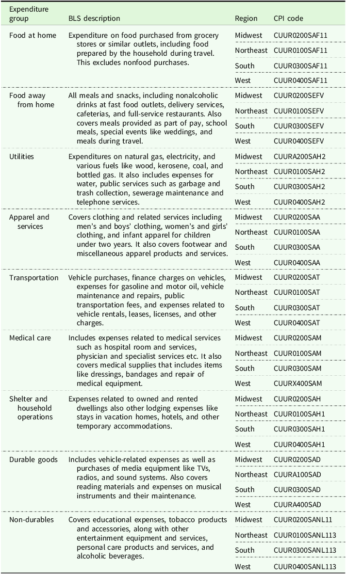
Source: BLS. We consider nine expenditure groups that are described in the table with their respective CPI code from each region.
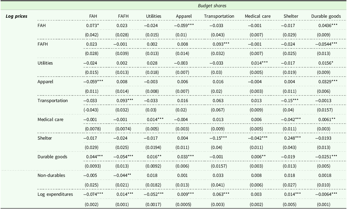
Demand system parameter estimates for log prices and expenditures
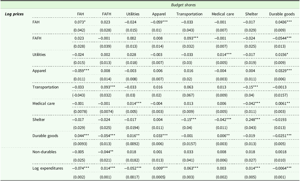
Table A2 Long description
The table presents demand system parameter estimates for log prices and expenditures across various budget shares. It includes 11 rows and 9 columns, with the first row and column containing headers and labels. The columns are labeled as FAH, FAFH, Utilities, Apparel, Transportation, Medical care, Shelter, Durable goods, and Log expenditures. The rows are labeled with the same categories. Each cell contains a numerical value followed by its standard error in parentheses. Notable trends include significant values marked with asterisks indicating levels of statistical significance. For example, the value 0.073* in the FAH row under the FAH column is significant at the 10 percent level, while 0.059*** in the Apparel row under the FAH column is significant at the 1 percent level. The table also includes a note about the use of balanced repeated replicate (BRR) weights and the inclusion of regional dummies in the model.
Standard errors in parentheses using balanced repeated replicate (BRR) weights. Model includes regional dummies (not reported) whose estimates are statistically insignificant.
The sample used is of 5,811 observations per variable from 2006 to 2022 across all regions in the US times number of equations (46,488 = 5,811 x 8). *p < 0.10, **p < 0.05, ***p < 0.010.



 Open access

