
INTRODUCTION
The Southern region of Ethiopia is endowed with suitable arable land and favourable climate well suited to the production of annual and perennial crops. However, it is also the most densely populated part of the country, making horizontal expansion of arable land an unsustainable source of output growth. The importance of agricultural technologies cannot, therefore, be emphasized enough for the region. In fact, there is no more effective driver of agricultural productivity than the use of modern agricultural technologies such as improved seeds and chemical fertilizers. However, in the region, not every crop is cultivated with the application of such inputs. For example, root and tuber crops such as sweet potato are usually cultivated with little or no application of such inputs. The vast majority of sweet potato producers in the region are producing sweet potato using mainly local varieties, family labour and manure. As a result, they have much lower yield of 6 to 8 Mg ha−1, although they can potentially provide over 50 to 60 Mg ha−1 (Markos and Loha, Reference Markos and Loha2016). The International Potato Centre reports that average yields of sweet potatoes in sub-Saharan Africa are 10-times lower among smallholders than those observed among commercial producers (International Potato Centre, 2016).
The challenge of increasing sweet potato output in the Southern region of Ethiopia is compounded by the fact that there is no much land left to bring under cultivation because of the high population density. In the absence of technological use and expansion of cultivation, sweet potato producers have no option but to continue operating under traditional farming. This then begs the question of whether or not it is feasible, and if so, to what extent additional output can be obtained in traditional sweet potato producers’ farms without additional inputs, given the existing traditional technology. Furthermore, how much room is left for cost savings through reallocation of the available inputs and existing traditional technology? To our knowledge, there are no empirical studies that have tried to look into the technical and allocative efficiency performance of sweet potato producers under traditional farming in the Southern region of Ethiopia. This study addresses three major research questions: Is there technical inefficiency among sweet potato producers in the Southern region of Ethiopia? Are sweet potato producers in the region optimally allocating their resources? What explains the variation in efficiency among sweet producers? These questions pertain to efficiency analysis of the use of the available resources. The first question pertains to the analysis of technical efficiency; the second question pertains to the analysis of allocative efficiency and the third question pertains to the analysis of the factors that contribute to the technical efficiency. Efficiency is about maximizing output from a given mix of inputs and existing technology, or producing a given level of output with minimum cost by adjusting the mix of inputs. Economic theory posits that producers are characterized as efficient if they can produce maximum output within the limit of their available resources (technical efficient) or whether they can produce that output with minimum cost (allocative efficient). Technical efficiency reflects the ability to obtain maximal output from a given set of inputs while allocative efficiency reflects the ability to use inputs in optimal proportions given the respective prevailing prices and available technology (Farrell, Reference Farrell1957). The product of technical and allocative efficiencies yields the level of economic efficiency (termed overall efficiency by Farrell) which is achieved when a producer combines resources in such a way as to generate maximum output (technical) while ensuring least cost to obtain maximum profit (allocative).
In order to address the above three research questions, the stochastic frontier production approach is applied. The first research question of whether or not there is technical inefficiency in sweet potato production was assessed by estimating the stochastic frontier Cobb–Douglas production function in log-linear functional form. The second research question of whether or not a given input is optimized was addressed by computing the efficiency points of utilization for each input based on the output–input price ratio and marginal product obtained from the Cob–Douglas production function. The third research question was addressed by estimating the efficiency scores generated from the Cob–Douglas production function as a function of farm-specific characteristics. Data came from a formal survey of 158 sweet potato producers conducted in Sodo–Zuria District, Southern region of Ethiopia formally known as the Southern Nations, Nationalities and Peoples Region (SNNPR). Sweet potato is widely produced in the densely populated parts of the region, thereby supporting the livelihood of millions of people in the region. Sweet potato is generally considered more productive, adaptable to marginal growing conditions, performs well under low input conditions (Oswald et al., Reference Oswald, Kapinga, Lemaga, Ortiz, Kroschel and Lynam2009), provides more edible energy per hectare per day than wheat, rice or maize and is also a major source of vitamin A (International Potato Centre). As such, it holds considerable potential for reducing hunger, malnutrition and poverty in the region.
MATERIALS AND METHODS
Analytical framework
In the literature of efficiency measurement, both parametric and non-parametric approaches are widely applied (Murillo-Zamorano, Reference Murillo-Zamorano2004). The parametric approach is further subdivided into deterministic and stochastic. The deterministic frontier production approach is motivated by the notion that all the deviations from the production frontier are under the control of the firm and hence, a result of the firm's inefficiency. Further, any specification problem is also considered as part of the inefficiency (Murillo-Zamorano, Reference Murillo-Zamorano2004). In contrast, the stochastic frontier production approach proposed independently by Aigner et al. (Reference Aigner, Lovell and Schmidt1977) and Meeusen and van den Broeck (Reference Meeusen and van den Broeck1977) is motivated by the notion that deviations from the production frontier might not be entirely under the control of the firm being studied. The deviations can also be attributed to a random component that reflects measurement error in the specification and estimation of frontier production functions.
The stochastic frontier production function proposed independently by Aigner et al. (Reference Aigner, Lovell and Schmidt1977) and Meeusen and van den Broeck (Reference Meeusen and van den Broeck1977) is expressed as
 $$\begin{equation}
{Y_i} = f\left( {{X_i},{\rm{\beta }}} \right){{\rm{e}}^\epsilon }
\end{equation}$$
$$\begin{equation}
{Y_i} = f\left( {{X_i},{\rm{\beta }}} \right){{\rm{e}}^\epsilon }
\end{equation}$$
where Yi represents the output of the ith farm, Xi represents the inputs used in the production process; β is a vector of parameter estimates; εi = vi − ui is composite error where vi is a two-sided (−∞ < v < ∞) random error component capturing the stochastic effects outside the farmer's control (e.g. policy changes, bad weather, drought, etc.) and accounting for effects of measurement error in the output variable and omitted variables, and ui represents the technical inefficiency effect of the farmer.
While the stochastic frontier production function as a measure of efficiency was welcome as a favourable development in the efficiency literature, the requirement for distributional assumption of the two error terms and explicit specification of the functional form of the production function was viewed as a price to pay (Coelli and Battese, Reference Coelli and Battese1996). In the literature, a number of distributions have been assumed with the most frequently used being half-normal (Aigner et al., Reference Aigner, Lovell and Schmidt1977), exponential (Meeusen and van den Broeck, Reference Meeusen and van den Broeck1977; Ng’ ombei and Kalindal, Reference Ng’ ombei and Kalindal2015) and truncated normal (Battese and Cora, Reference Battese and Cora1977; Ben and Ross, Reference Ben and Ross2002). There is no a priori argument that suggests that one form of distribution is superior to another, although different assumptions yield different efficiency levels (Chirwa, Reference Chirwa2007).
The maximum likelihood (ML) estimation of Eq. (1) yields the parameter estimates of β's and λ where λ = σu/σv. An assumption on the distribution of the error terms is needed to separate the composed error for efficiency analysis. Jondrow et al. (Reference Jondrow, Lovell, Materov and Schmidt1982) has shown that the expected value of ui conditional on the composed error εi under the assumption of half-normal distribution can be given as
 $$\begin{equation}
E\left[ {{u_i}|{\epsilon _i}} \right] = \frac{{\sigma \lambda }}{{\left( {1 + {\lambda ^2}} \right)}}\left[ {\frac{{\phi \left( {{\epsilon _i}\lambda /\sigma } \right)}}{{{\rm{\Phi }}\left( { - {\epsilon _i}\lambda /\sigma } \right)}} - \frac{{{\epsilon _{i\lambda }}}}{\sigma }} \right]
\end{equation}$$
$$\begin{equation}
E\left[ {{u_i}|{\epsilon _i}} \right] = \frac{{\sigma \lambda }}{{\left( {1 + {\lambda ^2}} \right)}}\left[ {\frac{{\phi \left( {{\epsilon _i}\lambda /\sigma } \right)}}{{{\rm{\Phi }}\left( { - {\epsilon _i}\lambda /\sigma } \right)}} - \frac{{{\epsilon _{i\lambda }}}}{\sigma }} \right]
\end{equation}$$
where ϕ is the density function of the standard normal distribution; Φ is the cumulative density function; λ = σu/σv and  $\ \sigma = \sqrt {\sigma _u^2 + \sigma _v^2} .$
Once the conditional estimates are obtained, the technical efficiency (TEi) of each producer can be computed as
 $$\begin{equation}
T{E_i} = 1 - E\left[ {{u_i}|{\epsilon _i}} \right]
\end{equation}$$
$$\begin{equation}
T{E_i} = 1 - E\left[ {{u_i}|{\epsilon _i}} \right]
\end{equation}$$
In terms of functional forms of production functions, the most common forms in the literature of efficiency analysis include Cobb–Douglas, constant elasticity of substitution (CES) and translog (transcendental logarithmic) functions. Of these, Cobb–Douglas has been the most widely applied functional form in stochastic frontier production analysis, largely because it is simple to apply (Ben and Ross, Reference Ben and Ross2002). However, its simplicity comes at the cost of some very restrictive assumptions, including the assumption that all firms operate at the same scale and that the marginal rate of input substitution, i.e., elasticities of substitution is unity (Coelli, Reference Coelli1995). Alternative forms such as the translog production function have been recommended. The translog function has a more flexible functional form than the Cobb–Douglas, imposing no restrictions on returns to scale and input substitution, but it is susceptible to multicollinearity. Likewise, because many more parameters are required than in an equivalent Cobb–Douglas model, larger data sets are required to avoid problems associated with degrees of freedom.
Given the distributional assumption required for the identification of the efficiency term, the parameters of stochastic frontier production functions are usually estimated by ML methods (Belotti et al., Reference Belotti, Daidon, Ilardi and Atella2012). In fact, they can also be estimated using corrected ordinary least squares (COLS). However, the ML estimator is asymptotically more efficient and should, therefore, be used in preference to the COLS estimator (Coelli, Reference Coelli1995).
In testing the null hypothesis of efficiency, the variance parameters are expressed as
 $$\begin{equation}
{{\rm{\sigma }}^2} = {\rm{\sigma }}_v^2 + {\rm{\sigma }}_u^2
\end{equation}$$
$$\begin{equation}
{{\rm{\sigma }}^2} = {\rm{\sigma }}_v^2 + {\rm{\sigma }}_u^2
\end{equation}$$
 $$\begin{equation}
\gamma = \ \sigma _u^2/{\sigma ^2}{\rm{\ }}
\end{equation}$$
$$\begin{equation}
\gamma = \ \sigma _u^2/{\sigma ^2}{\rm{\ }}
\end{equation}$$
The value of γ measures the total variation of output from the production frontier which can be attributed to technical inefficiency (Battese and Cora, Reference Battese and Cora1977). It ranges from 0 to 1, with values close to 1 indicating that the inefficiency component makes a significant contribution to the total variation of output from the production frontier (Coelli and Battese, Reference Coelli and Battese1996). If γ = 0, σ2u = 0 and σ2v = σ2, it means that the farm outputs differ from frontier outputs due to measurement errors and other external factors of production beyond the control of the farmer. On the other hand, if γ = 1, σ2v = 0 and σ2u =σ2, it means that the difference between farm outputs and frontier outputs is due to farm inefficiencies.
Beyond assessment of the level of efficiency, the stochastic frontier production function has been applied in the analysis of factors explaining the differences in technical inefficiency. In doing so, two main approaches (one-step and two-step) have been in use. The two-step approach entails the estimation of the stochastic frontier production function in the first stage, and prediction of the technical inefficiency effects in the second stage under the assumption that the inefficiency effects are identically distributed. However, Battese and Coelli (1995) argue that the two-step approach contradicts the assumption of identically distributed inefficiency effects made in the stochastic frontier. They propose a one-step simultaneous estimation approach in which both the stochastic frontier and the inefficiency effects model are simultaneously estimated. There is, however, no consensus in the literature as to which approach – the single or two-stage method – is more appropriate.
Technical efficiency analysis
The stochastic frontier Cobb–Douglas production is applied to analyse technical efficiency. Choosing the log-linear functional form, the stochastic frontier Cobb–Douglas production function for sweet potato can be given by
 $$\begin{equation}
Ln{Y_i} = ln{\rm{\ }}{{\rm{\beta }}_0} + \mathop \sum \limits_{j = 1}^4 {{\rm{\beta }}_j}Ln{X_{ji}} + {\epsilon _i}
\end{equation}$$
$$\begin{equation}
Ln{Y_i} = ln{\rm{\ }}{{\rm{\beta }}_0} + \mathop \sum \limits_{j = 1}^4 {{\rm{\beta }}_j}Ln{X_{ji}} + {\epsilon _i}
\end{equation}$$
where Ln Yi is the natural log of sweet potato output for the ith farm; j indexes the production inputs from 1 to 4; β0 is intercept; β1, β2, β3 and β4 are parameter estimates of X 1 (seed), X 2 (land), X 3 (labour) and X 4 (manure), respectively; εi = vi − ui is the composed error term where vi is a normally distributed disturbance with mean zero and constant variance N(0, σ2v), representing measurement and specification error and ui a one-sided disturbance representing technical inefficiency effects associated with the ith farm. These two error terms are assumed to be independent of each other and identically and independently distributed across observations.
Following Battese and Coelli (Reference Battese and Coelli1995), the inefficiency effects can be specified as an explicit function of a vector of producers’ characteristics Z given as
 $$\begin{equation}
{u_i} = \psi '\bm{Z} + \bm{\xi }
\end{equation}$$
$$\begin{equation}
{u_i} = \psi '\bm{Z} + \bm{\xi }
\end{equation}$$
where ξ is defined by the truncation of the normal distribution with zero mean and variance (σ2). In estimating Eq. (7), the two-step estimation approach is applied. In the first step, the stochastic frontier model (Eq. 6) is estimated from which the efficiency scores are generated and then the relationship between efficiency and producers’ characteristics is estimated. In the literature, the two-step estimation method is commonly applied.
Allocative efficiency analysis
Using the parameter estimates of βi in Eq. (6), we can compute the marginal product of input j (MPj) at the mean as
 $$\begin{equation}
M{P_j} = \frac{{\partial Y}}{{\partial {X_j}}} = {{\rm{\beta }}_j}\frac{{\overline {{Y_i}} }}{{\overline {{X_{ij}}} }}
\end{equation}$$
$$\begin{equation}
M{P_j} = \frac{{\partial Y}}{{\partial {X_j}}} = {{\rm{\beta }}_j}\frac{{\overline {{Y_i}} }}{{\overline {{X_{ij}}} }}
\end{equation}$$
where  $\bar{Y}$ is the geometric mean of sweet potato output; $\overline {{X_j}} $ is the geometric mean of input j.
In order to determine whether or not a given input is optimized, we computed the efficiency points of utilization for each input (AEj) by dividing the value of marginal product (VMPj = MPjPy) of the input by the marginal input cost of the corresponding input, which is equal to the price (Wj) of the corresponding input under a competitive market as
 $$\begin{equation}
A{E_j} = \frac{{VM{P_j}}}{{{W_j}}} = \frac{{M{P_j}{P_y}}}{{{W_j}}}
\end{equation}$$
$$\begin{equation}
A{E_j} = \frac{{VM{P_j}}}{{{W_j}}} = \frac{{M{P_j}{P_y}}}{{{W_j}}}
\end{equation}$$
If AEi = 1, then the input is optimally/efficiently used but if AEj < 1 then the jth input is over-utilized, or if AEj > 1 then the jth input is under-utilized.
Data, study design and measurement of variables
The data for this study came from 158 sweet potato producers randomly selected from the population of sweet producers in Sodo–Zuria district, which is among the high potential sweet potato producing districts in the Southern region of Ethiopia. A three-stage, clustered, random sampling procedure was applied, involving the selection of kebeles (the smallest administrative unit in Ethiopia), villages and producers. Out of 31 kebeles in Sodo–Zuria district, three (Bosa Kacha, Delbo Atwaro and Delbo Wogene) were selected. Then, a total of 11 villages were randomly selected from the list of villages in the three selected kebeles of which four came from Delbo Atwaro and Delbo Wogene each, and three from Bosa Kacha. Following the selection of the villages, a complete list of sweet potato producers in each village was obtained from the three kebeles Administration Offices. Then, 13 producers were randomly selected from each of the four selected village in Delbo Atwaro and Delbo Wogene, and 18 sweet potato producers from each village of Bosa Kacha, resulting in a sample of 158 producers. They account for nearly 0.5% of the total number of households in the three kebeles of the study district (32852) based on the latest census (CSA 2007). According to Bartlett et al. (Reference Bartlett, Kotrlik and Higgins2001), the minimum sample size needed for a population size of 4000 at 3% margin of error in the case of continuous variables such as yield (the variable of primary interest in our study) is 119.
Considering the size of the sample, we also tried to see how the values of some key socioeconomic variables in our sample such as household size, education and farm size parallel with those in a larger survey such as the Ethiopian Rural Socioeconomic Survey (ERSS) conducted in the Southern region of Ethiopia in 2011/12. The ERSS was implemented by the Central Statistical Authority of Ethiopia (CSA) in partnership with the World Bank Living Standards Measurement Study (LSMS) team as part of the Integrated Surveys on Agriculture Program (CSA and World Bank, 2013). According to this regional survey, the rural household size in the Southern region of Ethiopia is 5.3 members, compared to 5.5 members in our sample survey. The literacy rate in the Southern region of Ethiopia is 55.2%, compared to 60% in our sample. The average field size of a rural household in the Southern region is 0.88 ha, compared to 0.80 ha in our survey. Also, the size of a field, according to the regional socioeconomic survey, is 0.07 ha, compared to 0.11 ha allocated to a sweet potato field in our survey. The closeness of the values of these key variables between the two surveys can be attested by the fact that we had a careful consideration of the sampling frame and use of random sampling method in the study. It is known that representativeness has to do more with sampling frame than sample size.
Further, given that the ratio of the number of observations to independent variables in our efficiency model is 16, there is only minimal risk of the sample results not being generalized to the population. In using multiple regressions, the ratio of observations to independent variables should not fall below five (Bartlett et al., Reference Bartlett, Kotrlik and Higgins2001).
Data in the present study were collected on biophysical, demographic, socioeconomic and institutional characteristics of sweet potato producers through standardized questionnaires, which were administered to the selected producers in the 2013/14 production season. The data were collected by trained enumerators using tablets equipped with Surveybe software and exported to STATA 13 for stochastic frontier production, cost and other relevant statistical analysis. In the stochastic frontier production analysis, sweet potato output measured in megagram (Mg) constitutes the dependent variable. Planting materials, land, labour and manure constitute the independent variables. The data on planting materials were taken in local unit called eser, which, on average, consists of 550 vine cuttings and weighs 0.022 Mg. For convenience, planting materials are referred hereafter as seeds and expressed in Mg. As in the case with seeds, the data on land under sweet potato cultivation is also measured in a local unit called timad, which is equivalent to 0.25 ha. Labour is measured in man-days (MD) of family and hired labour used in the production of sweet potato. Manure is measured in Mg. Farm-specific variables are included in the efficiency effects model (Eq. 7). These include gender, age, education, household size (as a proxy for labour availability), livestock measured in tropical livestock unit (TLU) (as proxy for wealth), variety, extension, training and credit.
RESULTS AND DISCUSSION
Summary statistics of the stochastic frontier production and cost model variables
The mean sweet potato output per farm (0.11 ha) was 0.572 Mg, equivalent to 5.2 Mg ha−1 (Table 1). At an average sweet potato price of ETB 1,780 Mg−1, the total sweet potato revenue on an average farm was ETB 1018, amounting to total revenue of ETB 9256 ha−1. In terms of inputs, an average producer used 0.153 Mg of seeds, 13.5 MD of hired labour, 5.87 MD of family labour and 0.306 Mg of manure, which is equivalent to an estimated 1.39 Mg ha−1 of seeds, 122.73 MD ha−1 of hired labour, 53.36 MD ha−1 of family labour and 2.78 Mg ha−1 of manure, respectively. At the average land rental cost of ETB 2726 ha−1, seed cost of ETB 890.90 Mg−1, wage rate of ETB 36.25 MD−1 and manure cost of ETB 132.70 Mg−1, the estimated production cost of an average sweet potato producer is ETB 1178.94, which is equivalent to an estimated production cost of ETB 10717.60 ha−1. Labour cost accounts for over half of the total cost of sweet potato production (Table 1). As the sweet potato producers are traditional farmers, they are usually using their family labour, seeds and land. Thus, the above production costs included imputed (implicit) costs (i.e., costs of own factors of production). Given the total cost (implicit and explicit) and revenue, an average producer incurred a loss of about ETB 160.78, which is equivalent to an estimated loss of ETB 1461.60 ha−1. This shows that traditional sweet potato producers in the study area were operating at a loss, suggesting the need for adjustment of input use.
Table 1. Summary statistics of variables used in the production models.
Note: 1 ETB (Ethiopian Birr) = US$0.052 in end of 2013; MD: Man-day; Mg: Megagram.
The geometrical mean is used in the determination of the optimal level of the inputs in the allocative efficiency analysis.
Summary statistics of the efficiency effects model variables
The sample included both male-headed and female-headed households with the former accounting for the majority (77%). The average age of the sample producers was 46 years (Table 2). In terms of education, the majority (60%) did not have formal education. Only 26 and 14% had primary- and secondary-level education, respectively. The farm size of the sample producers ranged from 0.25 to 6.25 ha, with a mean of 0.8 ha. The average producer had 0.11 ha under sweet potato cultivation (Table 2). In the study area, a hectare of land can be rented for about 2726 year−1. The cultivation of improved sweet potato varieties was very limited and only about 6% of the farmers reported cultivating improved sweet potato varieties. Producers get access to extension services through formal training, extension visit and field demonstration. During the production season covered by the survey (2013/14), nearly 40% of producers reported to have been visited by extension agents (Table 2). About 22 and 26% reported to have received training and participated in on-farm demonstration, respectively. They reported receiving extension visits three times and attended training and demonstration trials once. As for access to credit, producers got access to credit from various sources such as saving and credit associations, micro-finance institutions (MFI), friends and relatives. About 36% of the producers reported to have had access to credit during the production season covered by the survey (Table 2). They reported taking an average loan of ETB 873 per person for a period of 11 months.
Table 2. Summary statistics of variables used in the efficiency effects model.
Technical efficiency
Table 3 reports results of the ML estimation of the stochastic frontier Cobb–Douglas production function (Eq. 6) implemented in the Frontier programme version 4.1 with STATA 13 (Coelli, Reference Coelli and Battese1996). The null hypothesis of no technical inefficiency in sweet potato production (H0: σ2u = 0) was tested against the alternative hypothesis (H1: σ2u > 0) using the generalized likelihood ratio test. The estimated value of λ = σu/σv = 2.90 was significantly different from 0 at 5% significance level, thus rejecting the null hypothesis of no inefficiency effects. This implies that inefficiency effects were important determinants of sweet potato output. The estimated value of γ derived from λ (γ = λ 2/(1 + λ 2) = σ2u/σ2) was 0.894, indicating that the inefficiency component makes a significant contribution (89.4%) to the total variation of output from the production frontier. As expected, the signs of the ML parameter estimate of the production inputs were all positive (Table 3). Among the four production inputs included in the model, three (land, labour and manure) were found to have statistically significant effects on sweet potato output. As the model is log-linear, the parameter estimates can be interpreted as partial output elasticities. The partial output elasticities associated with all the three statistically significant inputs were less than one, indicating that a given percentage increase in each input would result in less than proportional increase in sweet potato output. For example, a 1% increase in land, labour and manure yields a 0.47, 0.55 and 0.24% increase in sweet potato output, respectively. The returns to scale (sum of output elasticities) was 1.34, indicating that on average sweet potato production has increasing returns to scale (Table 3). The hypothesis that the sweet potato producers operate under a constant returns-to-scale technology was rejected (χ 2 = 18.28; P < 0.001). This implies that there is a proportionate cost savings gained by increased sweet potato production (economies of scale).
Table 3. ML estimates of the stochastic frontier Cob–Douglas production model.
*Significant at 0.1 level, **Significant at 0.05 level, ***Significant at 0.01 level.
Likelihood-ratio test of σu = 0: $\bar{\chi }_1^2 = 17.05$; $P \ge \bar{\chi }_1^2 = 0.00.$
Allocative efficiency
Table 4 indicates that producers’ utilization levels of seed, land and manure in the study area were away from the point of allocative efficiency. Economic theory states that the point of allocative efficiency (maximum profit) is reached when the value of marginal product (VMP) of an input is equal to its marginal input cost. The VMPs of land and manure were greater than their corresponding marginal input costs while that of seed was lower than its corresponding marginal input costs, indicating that sweet potato producers were making sub-optimal use of their production inputs. Land and manure were under-utilized while seed was over-utilized. This finding suggests that sweet potato producers can make additional profit if they can reallocate their current utilization of production inputs in such a way that they cultivate more land and apply more manure but reduce the seed rate. In order to determine the percentage by which producers can increase land and manure utilization but reduce seed rate, we used Eqs. (8) and (9). Substituting Eq. (8) into Eq. (9) for MP, we determined the optimal level of utilization of each input as
 $$\begin{equation}
A{E_j} = {\beta _j}\frac{{\bar{Y}}}{{\bar{X}}}\frac{{{P_y}}}{{{W_j}}}
\end{equation}$$
$$\begin{equation}
A{E_j} = {\beta _j}\frac{{\bar{Y}}}{{\bar{X}}}\frac{{{P_y}}}{{{W_j}}}
\end{equation}$$
Table 4. Estimates of allocative efficiency.
Given that the point of allocative efficiency is reached when AEi = 1, we set AEi = 1 in Eq. (10) and rearrange the terms therein such that the optimal level of each input  $( {{{\overline {\hat{X}} }_j}} )$ can be determined as
 $$\begin{equation}
{\overline {\hat{X}} _j} = {\beta _j}\bar{Y}\left( {{P_y}/{W_j}} \right)
\end{equation}$$
$$\begin{equation}
{\overline {\hat{X}} _j} = {\beta _j}\bar{Y}\left( {{P_y}/{W_j}} \right)
\end{equation}$$
Substituting the parameter estimates of the stochastic frontier production model given in Table 3, the price of sweet potato and that of the arithmetic mean of the corresponding input, we can compute the levels of the inputs at which profits can be maximized. For example, the optimal level of land was computed to be 0.18 ha, compared to the actual average size of 0.11 ha. Analogously, the optimal level of manure was determined to be 1.8 Mg, which is higher than the actual average of 0.3 Mg. This suggests that by increasing sweet potato farm from 0.11 to 0.18 ha (63.6% increase) and manure use from 0.3 to 1.8 Mg (six fold) the average producer can obtain additional profits. In the case of seeds, the producer should decrease the amount of seed use by 40% from 0.153 to 0.092 Mg. With seed price of ETB 890 Mg−1, the 40% cut in seed rate yields a cost saving of ETB 54.29 per farm. Since labour is optimized, there is no cost saving.
Distribution of technical efficiency scores
The technical efficiency of sweet potato producers ranged from 12.6 to 93.7%, with more than half (56%) of the producers having above the mean efficiency level in sweet potato production (Figure 1). The mean efficiency of sweet potato production was 66.1%, exhibiting a fairly large room for improvement. If the average producers are to achieve the technical efficiency level of the most efficient producers in the sample (93.7%), they can realize a 29.4% output gain. With the average producer having an output of 0.572 Mg, the 29.4% efficiency improvement yields 0.168 Mg in additional output per farm. This is not trivial, especially given that over two-fifths of the producers operate at below-average efficiency level (Figure 1). To put the output gain in perspective, the additional output gain of 0.168 Mg per farm resulting from the 29.4% efficiency improvement is enough to feed an average household of five members for about two weeks at 2100 kcal per capita per day.
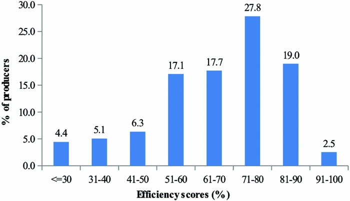
Figure 1. Distribution of technical efficiencies of sweet potato producers in Sodo–Zuria District, Southern region of Ethiopia.
Factors influencing technical efficiency
The efficiency model is estimated in a two-step process whereby the stochastic frontier Cobb–Douglas production function is first estimated to generate efficiency scores and then the generated efficiency scores are regressed on farm-specific characteristics presented in Table 2. The estimated efficiency model is tested for multicollinearity, heteroscedasticity, misspecification and goodness of fit. The test for multicollinearity is based on the variance inflation factor (VIF) and condition index (CI) values. The mean VIF of the predictors included in the model is 1.2, which is well within the acceptable range, suggesting a lack of multicollinearity. The problem of multicollinearity is present if the value of VIF is greater than 10 (Myer and Montgomery, Reference Myer and Montgomery1995) and the CI is equal to or greater than 30 (Belsley et al., 1980). The test for heteroskedasticity is conducted using the White's test, which indicated that heteroskedasticity is not a problem as evidenced by the failure to reject the null hypothesis of constant variance (χ2(58) = 54.11; P > χ(58)2 = 0.62). The test for model misspecification is conducted using the Ramsey RESET test. Results of the test indicated that model misspecification is not a problem. This is evidenced by the failure to reject the null hypothesis that states no omitted variables in the model [F (3144 = 1.48; P > F = 0.22)]. Tests of goodness of fit indicated a statistical significant F-test (F (10 147) = 6.91; P > F = 0.000), suggesting that the proposed relationship between the response variable and the set of predictors is statistically reliable.
Table 5 reports the parameter estimates of the factors hypothesized to explain the observed variation in producers’ technical efficiency. Among the 10 variables included in the model given in Eq. (7), four variables (Age, Education, Livestock and Extension) were found to have statistically significant effects (P < 0.1). Except for Extension, the three statistically significant parameters had positive signs as expected, indicating that the associated factors are efficiency increasing (Table 5). For example, the parameter estimate of Age was positive and statistically significant (P < 0.01), implying that all other factors held constant, age of the household head contributes to increasing efficiency. This can be explained by managerial skills acquired over time. The direct relationship between age and technical efficiency is supported by findings in Oladeebo and Fajuyigbe (Reference Oladeebo and Fajuyigbe2007). As in the case with Age, Education was also positively and significantly associated with efficiency of sweet potato production. That is, as number of years of schooling increases, the efficiency of sweet potato production increases. This result is consistent with the findings of several studies (Alene and Hassan, Reference Alene and Hassan2003; Battesse and Coelli, Reference Coelli1995). In a study on determinants of farm-level technical efficiency among adopters of improved maize production technology in Western Ethiopia, Alene and Hassan (Reference Alene and Hassan2003) found that technical efficiency is positively and significantly influenced by education.
Table 5. Determinants of technical efficiencies.
*Significant at 0.1 level, **Significant at 0.05 level and ***Significant at 0.01 level.
Consistent with expectation, the parameter's estimate for Livestock as measured by TLU is positive and statistically significant at 10% probability level. The plausible explanation is the fact that producers who own livestock can apply manure adequately and timely, and also get draught power for timely land preparation and additional cash income (to finance crop production). When it comes to Extension as measured by whether or not the farmer receives extension advice, an unexpected negative relationship was found between efficiency and extension visit. One plausible explanation is the unsuitability of the modern extension messages to the traditional farming systems in which the sweet potato producers in the study region operate. Extension agents are essentially advising against use of traditional management practises, directing their messages in favour of use of improved technologies. But, the sweet potato producers in the study area are not using improved technologies in their production.
The finding that age and education positively influence technical efficiency, while formal extension does the opposite, implies that the less efficient producers in the study area might rather benefit from an informal platform of local knowledge sharing with literate senior producers than from the formal extension programme deliverers. The parameter's estimate for credit, as measured by whether or not the producer had received loan during the cropping season preceding the survey year, had the expected positive sign (Table 5). However, it was not statistically significant, showing that access to credit does not have stronger effects on technical efficiency of sweet potatoes production. This can be explained by the fact that sweet potato producers are heavily relying on family labour and manure, not only on hired labour and chemical fertilizer. While access to credit generally allows sweet potato producers to overcome liquidity constraints, it does not appear that it plays a greater role in allowing them to use inputs like hired labour timely.
The other variables such as Gender, Farm size, Household size, Variety and Training were not statistically significant (Table 5). This implies, for example, that women farmers are as efficient or inefficient as men counterparts. As in the case with gender, no statistically significant difference in efficiency was detected between sweet potato producers having different land-size categories. This might be because in the study area, sweet potato producers were generally smallholders, there by exhibiting little variability in farm size. Since land size is very small, the available land can be effectively managed across the board with the marginal labour making no much difference. In the case of training, the lack of statistical significance is most probably due to the fact that the training is on modern agriculture while the producers are in reality practising traditional agriculture. As the training is incompatible with the farming system, it may not be surprising that the training does not influence efficiency in either way.
CONCLUSIONS
This study assesses the efficiency of sweet potato producers in Sodo–Zuria District located in the Southern region of Ethiopia by applying stochastic frontier Cobb–Douglas production function. Data came from a formal household survey of 158 producers and the study revealed the existence of fairly large technical inefficiency in sweet potato production. The inefficiency component made a significant contribution (89.4%) to the total variation of output from the production frontier. According to the allocative efficiency analysis, sweet potato producers were using land, manure and seed at sub-optimal levels. Seed was over-utilized whereas manure and land were under-utilized, suggesting the possibility of increasing profit by increasing the level of use of land and manure, and decreasing the amount of seeds. For maximum profit, the average level of land and manure should increase to 0.18 ha and 1.8 Mg from their actual average size of 0.11 ha and 0.3 Mg, respectively. In the case of seeds, the producer should decrease the amount of seed use by 40% from 0.153 to 0.092 Mg per farm. These findings support the notion that output gains and costs savings in sweet potato production are plausible under traditional farming by a more efficient use of the existing local resources.
In terms of the distribution of the efficiency scores, fairly large variations in efficiency among producers were found. The technical efficiency ranged from 12.6 to 93.7% with more than half of the producers having above the mean efficiency level in sweet potato production, exhibiting fairly large variations in efficiency among producers in using the resources available at their disposal. As the mean efficiency of sweet potato production was 66.1%, there is a fairly large room for improvement. In view of these findings, it is advisable to put in place appropriate extension intervention programmes that enable sweet potato producers to exploit the potential gains in sweet potato output through technical and allocative efficiency improvement. As the substantial variations in efficiencies among the producers imply that some producers are more innovative and knowledgeable than others in managing their sweet potato farms, one plausible strategy is to initiate a platform of local knowledge sharing services on innovative sweet potato management practises currently being applied by the most efficient producers in the region. Particularly, in view of the finding that age and education are important determinants of the efficiency of sweet potato producers, promoting such a platform in which literate senior farmers share their management experiences with the young and less efficient sweet potato producers presents a cost-effective opportunity for increasing sweet potato output in the region.


 Open access